Consistency of Lloyd’s Algorithm Under Perturbations

Abstract.

In the context of unsupervised learning, Lloyd’s algorithm is one of the most widely used clustering algorithms. It has inspired a plethora of work investigating the correctness of the algorithm under various settings with ground truth clusters. In particular, Lu and Zhou, (2016) have shown that the mis-clustering rate of Lloyd’s algorithm on $n$ independent samples from a sub-Gaussian mixture is exponentially bounded after $O(\log(n))$ iterations, assuming proper initialization of the algorithm. However, in many applications, the true samples are unobserved and need to be learned from the data via pre-processing pipelines such as spectral methods on appropriate data matrices. We show that the mis-clustering rate of Lloyd’s algorithm on perturbed samples from a sub-Gaussian mixture is also exponentially bounded after $O(\log(n))$ iterations under the assumptions of proper initialization and that the perturbation is small relative to the sub-Gaussian noise. In canonical settings with ground truth clusters, we derive bounds for algorithms such as $k$-means$++$ to find good initializations and thus leading to the correctness of clustering via the main result. We show the implications of the results for pipelines measuring the statistical significance of derived clusters from data such as SigClust (Liu et al.,, 2008). We use these general results to derive implications in providing theoretical guarantees on the misclustering rate for Lloyd’s algorithm in a host of applications, including high-dimensional time series, multi-dimensional scaling, and community detection for sparse networks via spectral clustering.

1. Introduction

Clustering seeks to partition a set of objects into different clusters or groups based on some measure of similarity. The $k$-means clustering technique aims to cluster a set of $n$ points, $\left\{\bm{y}_{i}:i\in[n]\right\}\subseteq\mathbb{R}^{r}$, with index set $[n]:=\{1,\ldots,n\}$, into $K\geq 1$ clusters, $\mathcal{C}_{1},...,\mathcal{C}_{K}$, via minimizing the cost function,

$$Cost(\bm{C}):=\sum_{k=1}^{K}\dfrac{1}{n_{k}}\sum_{\bm{y}_{i},\bm{y}_{j}\in\mathcal{C}_{k}}\|\bm{y}_{i}-\bm{y}_{j}\|^{2},$$ (1)

where $\bm{C}=\{\mathcal{C}_{1},\dots,\mathcal{C}_{K}\}$ is a candidate cluster, $n_{k}=|\mathcal{C}_{k}|$ for $k\in[K]$ are the corresponding cluster sizes, and $\|\cdot\|$ is the Euclidean distance. Minimizing the cost function is equivalent to minimizing the distance within clusters. Define $\bm{\mu}_{k}=\bm{\mu}_{k}(\bm{C})$ as the mean of the $n_{k}$ points in $\mathcal{C}_{k}$, where we suppress dependence on $\bm{C}$ to ease notational overhead. Then, (1) is equivalent to

$$Cost(\bm{C})=\dfrac{1}{n}\sum_{i=1}^{n}\|\bm{y}_{i}-\bm{\mu}_{z_{i}}\|^{2}$$

where $z:[n]\to[K]$ is the cluster assignment function given by $z(i)=k$ if $i\in\mathcal{C}_{k}$. We write $z_{i}$ for $z(i)$. Thus, the $k$-means optimization problem can be rewritten as

$$\min_{\bm{C},z}\dfrac{1}{n}\sum_{i=1}^{n}\|\bm{y}_{i}-\bm{\mu}_{z_{i}}\|^{2}.$$ (2)

The $k$-means optimization problem is NP-hard (Mahajan et al.,, 2009) and has motivated an enormous body of work in developing approximation schemes for (2), quite often via iterative schemes by first initializing a set of candidate means, then iterating between updating cluster assignments and updating cluster means until one converges to at least a local minima of the above cost function.

One of the most popular and simplest algorithms is Lloyd’s algorithm (Lloyd,, 1982), often referred to as the standard or naive $k$-means. The updating step in Lloyd’s algorithm is as follows. Let $\{\widehat{\bm{\mu}}^{(s)}_{k}\}$ be the estimated means of the cluster assignments at the $s$-th iteration. Then the estimated cluster assignment of $\bm{y}_{i}$ at the $(s+1)$-th iteration is given by

$$\widehat{z}^{(s+1)}_{i}=\mathop{\mathrm{argmin}}_{k\in[K]}\|\bm{y}_{i}-\widehat{\bm{\mu}}^{(s)}_{k}\|.$$ (3)

Lloyd’s algorithm always converges to a local minimum of (2) but the resulting clusters are heavily reliant on the initialization of the algorithm. Many other variations of the $k$-means algorithm have been proposed to speed up convergence and decrease computation times (Sarma et al.,, 2012), deal with data on specific domains (Wei et al.,, 2010), extend to soft clustering settings (Dunn,, 1973) and pick optimal initial centers (Arthur and Vassilvitskii,, 2007). Methods for optimizing (2) under different norms also exist, leading to other well-known algorithms such as $k$-medians (Arora et al.,, 1998) and $k$-medoids (Kaufman and Rousseeuw,, 2009). See Wierzchoń and Kłopotek, (2018) and the references therein for a general survey of such algorithms.

Although $k$-means is widely used in diverse applications, there is much less known about the convergence of $k$-means algorithms to the global optimum, or the correctness of the global optimum in settings with ground truth clusters. Under independent sampling from a mixture model and assuming a uniqueness condition of the population version of the cost function, Pollard, (1981) shows the consistency of $k$-means clustering and Pollard, (1982) proves a central limit theorem (CLT) for the cluster means of the optimal solution. Note that the results of Pollard, (1981, 1982) apply to the optimal solution of (2) and not necessarily to the (local) optima obtained by $k$-means algorithms. When there is only one global optimizer, the $k$-means algorithm is shown to be stable in the sense that $k$-means run on two samples of the same distribution yield arbitrarily close clusterings as the sample size increases (Rakhlin and Caponnetto,, 2007). Furthermore, multiplicative perturbation stability is shown in Awasthi et al., (2012), and additive perturbation stability is shown in Dutta et al., (2017) under the assumption of a large enough gap between clusters.

In settings with ground truth clusters, the misclustering rate, namely the proportion of misclustered points, is often used to quantify the accuracy of a proposed $k$-means algorithm. A canonical example is independent sampling from a mixture model; here Lu and Zhou, (2016) have shown the misclustering rate of Lloyd’s algorithm, given a good enough initial clustering, has an exponential bound after $O(\log n)$ iterations in the following setting. More precisely, it is assumed that the data are generated from a mixture distribution consisting of $K$ sub-Gaussian mixing distributions, and assumptions are made on the separation of (population) cluster means measured as the maximal distance between the means of the mixing distributions. This setting assumes that we directly observe the samples from the mixing distribution.

1.1. Informal description of our results

Here we briefly summarize the main contributions of this paper:

1. Theoretical analysis of iterative schemes under perturbed data: In the last decade, there has been significant interest, especially in the statistics community, in rigorously understanding iterative schemes such as EM-algorithm (Balakrishnan et al.,, 2017) and Lloyd’s algorithm (Lu and Zhou,, 2016); see the scholarly treatment with extensive references (Gao and Zhang,, 2022) for a broad recent overview of this area. In many situations, unsupervised learning algorithms such as Lloyd’s algorithm are not directly applied to the original data but rather pre-processed versions of the same; this could be owing to lack of access to the original data, for example, where these objects are loading vectors for factors in high-dimensional time series data, or due to dimension reduction pipelines such as Principal Component Analysis (PCA) and Multidimensional scaling (MDS) widely used in settings such as spectral clustering. Such issues lead to clustering estimates of the original data points, which introduces an estimation error, typically dependent across the points, as the entire data set is used for such estimation pipelines. The goal of this paper is to understand the correctness of Lloyd’s algorithm in such perturbed settings. In the sub-Gaussian mixture settings, with small enough perturbation, via a careful modification of the original proof in Lu and Zhou, (2016), we show that the misclustering rate of Lloyd’s algorithm has an exponential bound after $\mathcal{O}(\log n)$ iterations. Our main theorem reduces to the one used in Lu and Zhou, (2016) as a special case.

2. Properties of initialization generating algorithms: The main result requires control both on the level of perturbation as well as moderate control on the initialization of the algorithm. We provide (lower) bounds for algorithms such as $k$-means$++$ (Arthur and Vassilvitskii,, 2007) to provide such initializations, thus implying, using the main result, that Lloyd’s algorithm coupled with such initialization schemes have good properties, including recovery of clusters in the presence of ground truth clusters.

3. Significance of clusters: Over the last decade, there has been significant effort in formulating a methodology for testing the statistical significance of found clusters in unsupervised learning approaches (Liu et al.,, 2008; Shen et al.,, 2023). We show the implications of the results in this paper, in particular showing consistency of methodologies such as SigClust (Liu et al.,, 2008) for detecting and judging the presence of ground truth clusters.

4. Canonical applications: We illustrate the implications of the main results in a number of applications, including high-dimensional time series driven by underlying low-rank factors, high-dimensional data that undergo an initial dimension reduction step such as MDS and community detection for networks with latent low-rank structures.

1.2. Organization of the paper

Section 2 below describes the notation used in the paper. Then in Section 3, we introduce the general clustering framework studied in this paper. In Section 4, we state and prove the main results, while Section 5 has applications of the main results in a number of settings. Lastly, Section 6 contains the proofs of the main results while Section 7 contains proofs of the applications.

2. Notation

All vectors in this paper will be treated as column vectors. Unless otherwise stated, we will use $\|\bm{x}\|$ to denote the Euclidean $2$-norm of a vector $\bm{x}\in\mathbb{R}^{r}$ and for two vectors $\bm{x}_{1},\bm{x}_{2}\in\mathbb{R}^{r}$ write $\langle\bm{x}_{1},\bm{x}_{2}\rangle:=\bm{x}_{1}^{\top}\bm{x}_{2}$ for the inner product between these two vectors. For square matrix $\mathbf{A}\in\mathbb{R}^{r\times r}$, write $\|\mathbf{A}\|$ for the spectral norm of $\mathbf{A}$. The $2\rightarrow\infty$ bound for any matrix $\mathbf{X}\in\mathbb{R}^{n\times m}$ is defined as

$$\|\mathbf{X}\|_{2\to\infty}=\max_{i\in n}\|\mathbf{X}_{i}\|,$$

where $\mathbf{X}_{i}\in\mathbb{R}^{m}$ is the column vector corresponding to the $i$-th row of $\mathbf{X}$. Let $\lambda_{j}(\mathbf{A})$, $\lambda_{\max}(\mathbf{A})$ and $\lambda_{\min}(\mathbf{A})$ be the $j$-th largest, maximal and minimal eigenvalues of any real symmetric matrix $\mathbf{A}$. For any finite set $S$, write $|S|$ for the cardinality of $S$. A random vector $\mathbf{X}\in\mathbb{R}^{r}$ is said to be sub-Gaussian with parameter $\sigma>0$, denoted as subG($\sigma^{2}$), if for all $\bm{a}\in\mathbb{R}^{r}$,

$$\mathbb{E}e^{\langle\bm{X}-\operatorname{\mathds{E}}\mathbf{X},\bm{a}\rangle}\leq e^{\frac{\sigma^{2}\|\bm{a}\|^{2}}{2}}.$$

For sequences $\left\{a_{n}\right\}$ and $\left\{b_{n}\right\}$, we write $a_{n}=o\left(b_{n}\right)$ or $a_{n}\ll b_{n}$ if $\lim_{n}a_{n}/b_{n}=0$, and write $a_{n}=O\left(b_{n}\right),a_{n}\lesssim b_{n}$ or $b_{n}\gtrsim a_{n}$ if there exists a constant $C$ such that $a_{n}\leq Cb_{n}$ for all $n$. We write $a_{n}=w(b_{n})$ if $b_{n}=o(a_{n})$ and $a_{n}=\Omega(b_{n})$ if $b_{n}=O(a_{n})$. We write $a_{n}=\Theta(b_{n})$ if $a_{n}=O(b_{n})$ and $a_{n}=\Omega(b_{n})$. We write $a_{n}\asymp b_{n}$ if $a_{n}\lesssim b_{n}$ and $a_{n}\gtrsim b_{n}$. We write $o_{P}(\cdot),O_{P}(\cdot)$ for the corresponding probabilistic analogs, so for example, for a sequence of random variables $(X_{n};\,n\geq 1)$ and constants $(b_{n}:n\geq 1)$ with $b_{n}\uparrow\infty$, we write $X_{n}=o_{P}(b_{n})$ when $X_{n}/b_{n}\stackrel{{\scriptstyle\mathrm{P}}}{{\longrightarrow}}0$ as $n\rightarrow\infty$. Throughout, $C,C_{1},C_{2},\ldots$ are constants that can change from line to line. We let $\stackrel{{\scriptstyle\mathrm{w}}}{{\longrightarrow}}$, $\stackrel{{\scriptstyle\mathrm{P}}}{{\longrightarrow}}$, and $\stackrel{{\scriptstyle\mathrm{a.s.}}}{{\longrightarrow}}$ respectively denote convergence in distribution, convergence in probability, and almost sure convergence.

3. Ground truth template

Fix $K\geq 2$. Suppose $\{\bm{y}^{*}_{i}\}_{i\in[n]}$ are independent samples from a $K$-mixture distribution $\mathcal{F}$. More precisely, let $\bm{p}=\{p_{k}:k\in[K]\}$ be a probability mass function (with each component strictly positive) and let $\{\mathcal{F}_{k}:k\in[K]\}$ be $K$ sub-Gaussian probability measures on $\mathbb{R}^{r}$ each with sub-Gaussian parameter $\sigma>0$ (we will later make assumptions on the minimal separation of the population means of these clusters). Define $\mathcal{F}$ to be the mixture distribution,

$$\mathcal{F}=\sum_{k=1}^{K}p_{k}\mathcal{F}_{k}.$$ (4)

Next, let $\bm{y}^{*}_{i}\sim\mathcal{F}$ independent across $i\in[n]$. Let $z:[n]\to[K]$ be the membership function where $z_{i}=k$ if and only if $\bm{y}^{*}_{i}\sim\mathcal{F}_{k}$. If $z_{i}=k$, we say that $i$ belongs to the $k$-th cluster. Write $\bm{\mu}_{k}:=\mathbb{E}\mathcal{F}_{k}$ for the population mean of the $k$-th component of the mixture. Then we write

$$\bm{y}^{*}_{i}=\bm{\mu}_{z_{i}}+\bm{w}_{i},$$ (5)

where $\left\{\bm{w}_{i},i\in[n]\right\}$ are independent zero mean sub-Gaussian vectors with parameter $\sigma>0$. We assume that we do not observe the true samples $\{\bm{y}^{*}_{i}\}_{i\in[n]}$ and instead observe a perturbed sample $\{\bm{y}_{i}\}_{i\in[n]}$ given by

$$\bm{y}_{i}=\bm{y}^{*}_{i}+\bm{e}_{i}=\bm{\mu}_{z_{i}}+\bm{w}_{i}+\bm{e}_{i},$$ (6)

where $\{\bm{e}_{i}\}_{i\in[n]}$ is some (potentially dependent across $i$) noise assumed to be uniformly bounded by (a problem dependent) parameter $\epsilon$, i.e.,

$$\max_{i\in[n]}\|\bm{e}_{i}\|\leq\epsilon.$$ (7)

In our application settings, we will have high probability bounds on the event in question corresponding to (7). Let $\mathbf{Y}=(\bm{y}_{1},\ldots,\bm{y}_{n})^{\top}\in\mathbb{R}^{n\times r}$ be the observation matrix. Let $\mathbf{Z}\in\mathbb{R}^{n\times K}$ be the true membership matrix with $\mathbf{Z}_{i,k}=1$ if $z_{i}=k$ and $0$ otherwise. Let $\mathbf{M}=(\bm{\mu}_{1},\ldots,\bm{\mu}_{K})^{\top}\in\mathbb{R}^{K\times r}$ be the cluster center matrix. Let $\mathbf{E}=\mathbf{E}_{1}+\mathbf{E}_{2}$, where $\mathbf{E}_{1}=(\bm{e}_{1},\ldots,\bm{e}_{n})^{\top}$ and $\mathbf{E}_{2}=(\bm{w}_{1},\ldots,\bm{w}_{n})^{\top}$. Then the model in (6) can be written in matrix form as

$$\mathbf{Y}=\mathbf{Z}\mathbf{M}+\mathbf{E}=\mathbf{Z}\mathbf{M}+\mathbf{E}_{1}+\mathbf{E}_{2},$$ (8)

with $\|\mathbf{E}_{1}\|_{2\rightarrow\infty}\leq\epsilon$ and $\mathbf{E}_{2}$ row-independent sub-Gaussian matrix with $\sigma>0$. The model can be summarized by four driving ingredients $\{\mathbf{Z},\mathbf{M},\epsilon,\sigma\}$. We view $\bm{y}_{i}$ as an at most $\epsilon$ perturbed observation of $\bm{y}_{i}^{*}$. One may also view $\bm{y}_{i}$ as an estimate of $\bm{y}^{*}_{i}$ under the condition that $\|\bm{y}_{i}-\bm{y}_{i}^{*}\|\leq\epsilon$. Although assumption (7) appears restrictive, owing to foundational recent advances in high-dimensional statistics and probability (see e.g. Abbe et al., (2020, 2022) and the references therein) as described in Section 5, there are many settings in which such bounds can be obtained with high probability. It is worth noting that $k$-means clustering is invariant under a rotation. Therefore the performance of Lloyd’s algorithm on $\mathbf{Y}$ is the same as that on $\mathbf{Y}\mathbf{O}$ for any orthonormal matrix $\mathbf{O}$. For the rest of the paper, we will write $\mathcal{X}=\left\{\bm{y}_{i}\right\}_{i\in[n]}$, for the data that will be clustered; the underlying model will always be clear from the context.

4. Main Results

We start by describing the main results of this paper, deferring applications to the next section.

4.1. Clustering misclassification bounds

For $k\in[K]$, write $\mathcal{C}_{k}=\left\{i:z_{i}=k\right\}$ for the true $k$-th cluster and recall that $n_{k}=\left|\mathcal{C}_{k}\right|$ denotes the corresponding cluster size. For the minimal cluster density, write

$$\alpha=\min_{k\in[K]}\frac{n_{k}}{n}.$$ (9)

Let $\{\widehat{\bm{\bm{\mu}}}_{k}^{(s)}\}$ and $\widehat{z}^{(s)}$ be the estimated cluster centers and membership function respectively, after $s\geq 0$ iterations of Lloyd’s algorithm applied to $\{\bm{y}_{i}\}_{i\in[n]}$. The initial centers and corresponding membership function correspond to the $s\equiv 0$ setting. For any $l,k\in[K]$, define,

$$U_{lk}^{(s)}=\{i:z_{i}=l,\widehat{z}_{i}^{(s)}=k\}$$ (10)

as the subset of samples in cluster $l$ which are assigned to cluster $k$ at the $s$-th iteration. Note that the cardinality of these sets determines the number of misclustered points. Let $\widehat{n}_{lk}^{(s)}=|U_{lk}^{(s)}|$ and $\widehat{n}_{k}^{(s)}=|\{i:\widehat{z}_{i}^{(s)}=k\}|$. Denote the misclustering rate at iteration $s$ as

$$A_{s}=\min_{\pi\in S_{K}}\frac{1}{n}\sum_{i=1}^{n}\mathbb{I}\{\widehat{z}_{i}^{(s)}\neq\pi(z_{i})\},$$ (11)

where $S_{K}$ is the group of permutations on $[K]$. Assuming the cluster labels have been aligned such that $\pi(i)=i$, we can write the misclustering rate as

$$A_{s}=\frac{1}{n}\sum_{l,k\in[K]:l\neq k}\widehat{n}_{lk}^{(s)},$$

and the cluster-wise misclustering rate at iteration $s$ as

$$G_{s}=\max_{k\in[K]}\left\{\frac{1}{\widehat{n}_{k}^{(s)}}\sum_{l\neq k}\widehat{n}_{lk}^{(s)},\frac{1}{n_{k}}\sum_{l\neq k}\widehat{n}_{kl}^{(s)}\right\}.$$ (12)

The misclustering rate $A_{s}$ denotes the number of points incorrectly clustered after $s$ steps of Lloyd’s algorithm and $G_{s}$ denotes the maximum, over all clusters, of the proportion of points incorrectly placed in a cluster or the proportion of points in a cluster that were misclustered. Note that both $A_{s},G_{s}\leq 1$ and $G_{s}\alpha\leq A_{s}$.

In order to obtain bounds on the misclustering rate, we now describe assumptions required on the mixture distribution $\mathcal{F}$ such as separability of the means as well as signal-to-noise ratio. Define the minimal and maximal distance between the true population cluster means as

$$\Delta=\min_{l\neq k}{\|\bm{\mu}_{l}-\bm{\mu}_{k}}\|\quad\text{and}\quad M=\max_{l\neq k}{\|\bm{\mu}_{l}-\bm{\mu}_{k}}\|.$$ (13)

Define the scaled maximum of the mean estimation error at iteration $s$ as

$$\Gamma_{s}=\max_{k\in[K]}\frac{\|\widehat{\bm{\bm{\mu}}}_{k}^{(s)}-\bm{\bm{\mu}}_{k}\|}{\Delta}.$$ (14)

Define the signal-to-noise ratio,

$$\rho_{\sigma}=\frac{\Delta}{\sigma}\sqrt{\frac{\alpha}{1+\frac{Kr}{n}}},\quad\rho_{\epsilon}=\frac{\sqrt{\alpha}\Delta}{\epsilon}.$$ (15)

If $\sigma=0$ or $\epsilon=0$, we will let $\rho_{\sigma}=\infty$ or $\rho_{\epsilon}=\infty$, respectively. Note that both $\rho_{\sigma}$ and $\rho_{\epsilon}$ increase if the distance between the mixture means $\{\bm{\mu}_{k}\}_{k\in[K]}$ increases. If each component of the mixture distributions is more concentrated around their respective means, then $\rho_{\sigma}$ increases. Similarly, if there is less perturbation error $\epsilon$, then $\rho_{\epsilon}$ increases. So with large enough $\rho_{\sigma}$ and $\rho_{\epsilon}$, one would expect Lloyd’s algorithm to do well. However, as discussed in Section 1, $k$-means is reliant on a good initialization. We require that the initialization satisfies one of the following two conditions:

$$G_{0}\leq\left(\dfrac{1}{2}-\frac{\sqrt{6}+1}{\rho_{\sigma}}-\frac{2.1\sqrt{\alpha}+1}{\rho_{\epsilon}}-\frac{1}{\alpha^{1/4}}\sqrt{\frac{\sigma}{\Delta}}\right)\dfrac{\Delta}{M}\quad\text{or}\quad\Gamma_{0}\leq\frac{1}{2}-\frac{1}{\rho_{\sigma}}-\frac{1.1\sqrt{\alpha}+1}{\rho_{\epsilon}}-\frac{1}{\alpha^{1/4}}\sqrt{\frac{\sigma}{\Delta}}.$$ (16)

Similar conditions on the initialization in the zero perturbative noise ($\epsilon\equiv 0$) were first described in Lu and Zhou, (2016). The above conditions implicitly impose some restrictions on the driving parameters of the model. Note that as $\rho_{\sigma}$ or $\rho_{\epsilon}$ increases, the stringency imposed by the above conditions on the initialization weakens. The bound on $G_{0}$ is a requirement on our initial cluster assignments while the bound on $\Gamma_{0}$ states that the initial cluster mean estimates should not deviate too far from the true means relative to $\Delta$.

Given the initialization condition and upper bound on the additive perturbation $\epsilon$, the next result shows an exponential bound on the misclustering rate $A_{s}$ for $s=\Theta(\log{n})$ with probability at least $1-\delta$, where $\delta$ is an explicit error bound with dependence on $n,\sigma,\Delta,\rho_{\sigma},\rho_{\epsilon}$, given by

$$\delta(n,\sigma,\Delta,\epsilon)= \frac{1}{n}+2\exp\left(-\frac{\Delta}{\sigma}\right)+2\exp\left(-\frac{\Delta}{\sqrt{\epsilon\sigma}}\right).$$

Note that $\delta\to 0$ as $\rho_{\sigma},\rho_{\epsilon},n\to\infty$.

Theorem 4.1.

Assume that

$$n\alpha \geq C_{1}K\log n,$$ (17)

$$\rho_{\sigma} \geq C_{2}\sqrt{K},$$ (18)

$$\rho_{\epsilon} \geq C_{3}\sqrt{K},$$ (19)

$$\frac{\Delta^{2}}{\epsilon\sigma} \geq r\log(3),$$ (20)

for some sufficiently large constants $C_{1},C_{2},C_{3}>0$. Assuming the initialization satisfies (16), we have

$$A_{s}\leq\max\left\{\exp\left(-\dfrac{\Delta^{2}}{16\sigma^{2}}\right),\exp\left(-\frac{\Delta^{2}}{8\epsilon\sigma}\right)\right\}\quad\text{for all}\quad s\geq 4\log n$$ (21)

with probability greater than $1-\delta(n,\sigma,\Delta,\epsilon)$.

Remark 4.1.

The noiseless setting “$\epsilon\equiv 0$” was analyzed in a fundamental paper by Lu and Zhou, (2016). One main goal of this paper is to show how the proof techniques developed in that paper carry over to settings with additive perturbation. However, carrying out this program leads to a number of major challenges, including dealing with three parts of error: the sub-Gaussian error, the random perturbation error, and their interaction in each iterative step of Lloyd’s algorithm. This necessitates a different decomposition of functionals such as $A_{s}$ as well as various technical Lemmas describing the concentration of required empirical averages around their population values. Extending the entire framework to the near discrete setting in the context of community detection of sparse network models, with degrees scaling like $\Theta(\log{n})$ (described in the next section) leads to further technical challenges.

Remark 4.2.

Note that the bound on the misclustering rate depends on both effective signal-to-noise ratios. The max term in the error bound indicates that it is not good enough to have just one of these terms be small. We must have small enough perturbation and sub-Gaussian error relative to $\Delta$ for Lloyd’s algorithm to work well. Further, as should be intuitively clear, as the distance between the population means gets smaller, we require a smaller additive perturbation error $\epsilon$ and smaller sub-Gaussian error $\sigma$ for a better probability. Finally, we note that the proof of Theorem 4.1 has not been optimized to find the lowest constants $C_{1},C_{2},C_{3}>0$ such that the result holds. Although the current proof uses some quite large constants $C_{1},C_{2},C_{3}>0$, our simulations show that the constants can be much smaller in practice.

Remark 4.3.

The initialization conditions given in (16) ensure that the initialized means are not too far away from the true means. Consider the case when $K=2$. Then the condition on $\Gamma_{0}$ yields that the initial means $\widehat{\bm{\mu}}^{(0)}_{1},\widehat{\bm{\mu}}^{(0)}_{2}$ must be at most $\frac{1}{2}\Delta$ distance away from $\bm{\mu}_{1},\bm{\mu}_{2}$, respectively. As the signal-to-noise ratios increase, the distances are allowed to approach $\frac{1}{2}\Delta=\frac{1}{2}\|\bm{\mu}_{1}-\bm{\mu}_{2}\|$. Note that even though the initial condition on $G_{0}$ is a bound on the cluster-wise misclustering rate, we have shown in the proof of Theorem 4.1 that the condition on $G_{0}$ implies the condition on $\Gamma_{0}$ in this setting. This is not surprising since good initial cluster labels should indicate that the means are relatively close to the true means.

Remark 4.4.

Even with large signal-to-noise ratios, without the initial conditions (16), Lloyd’s algorithm may arrive at a local minimum different from the global minimum. A theoretical example is given by Lu and Zhou, (2016), showing that (16) is almost necessary. In Figure 1, we provide an example where $\sigma=0$, $\epsilon=1$, and $\Delta=2\sqrt{2}$. But with initial means not satisfying (16), Lloyd’s algorithm converges to a local optimum which yields a bad misclustering rate.

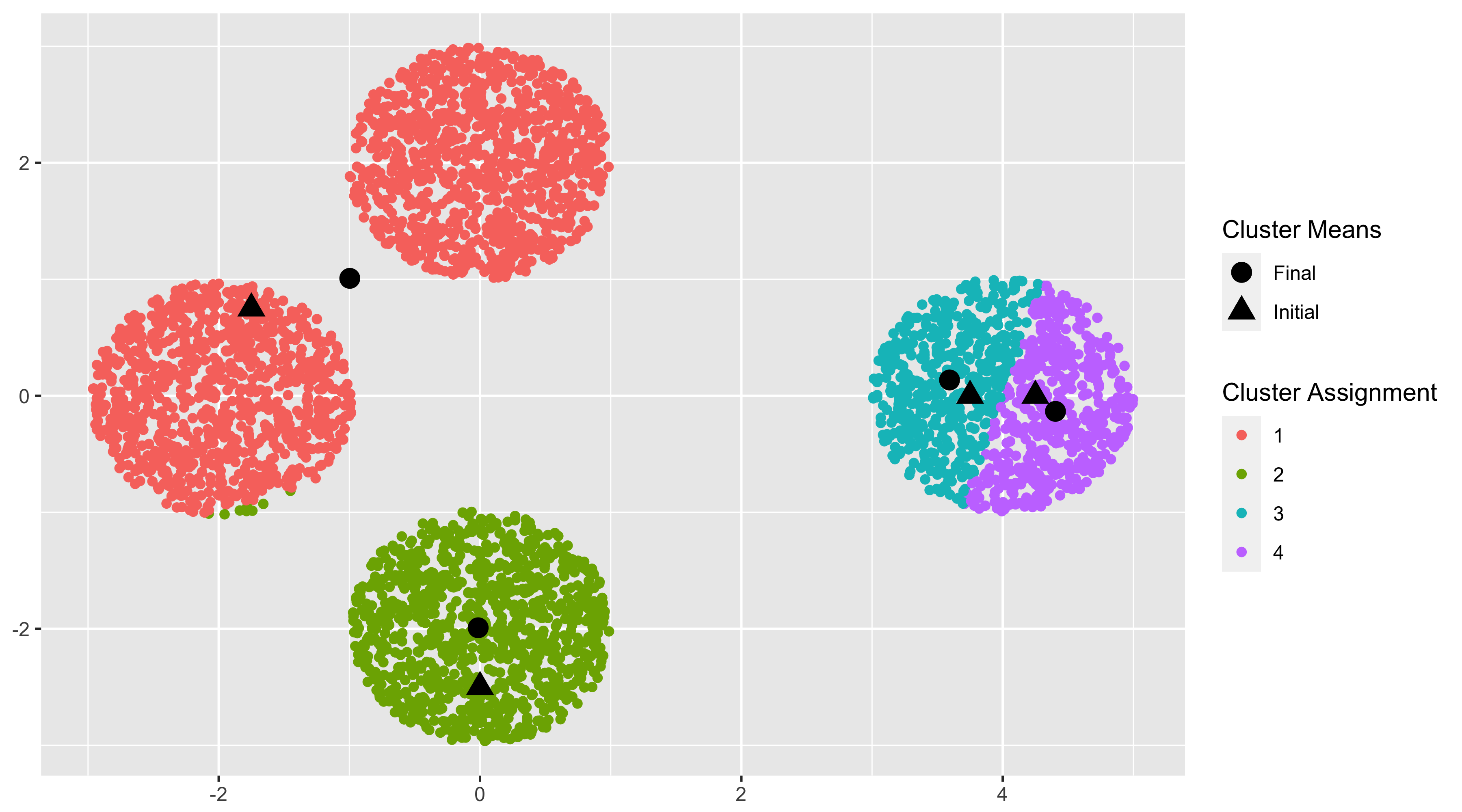
Figure 1. An example illustrating the need for the initial conditions given in (58). Note that even with clear separation of the four clusters, there exist candidate initial means which lead to local optima with a bad misclustering rate.

As a byproduct of Theorem 4.1, we have the convergence rate of estimated cluster centers under our proposed model. A similar result was stated in Lu and Zhou, (2016, Theorem 6.2), but our results seem to indicate the presence of an additional error term in the error bound.

Corollary 4.2.

Assume conditions (17) - (20) hold for some sufficiently large constants $C_{1},C_{2},C_{3}>0$. Then given any initializer satisfying (16), we have for $s\geq 4\log n$,

$$\max_{k\in[K]}\|\widehat{\bm{\mu}}^{(s)}_{k}-\bm{\mu}_{k}\|\leq 2\sqrt{3}(\sqrt{K}+1)\sigma\sqrt{\dfrac{(n+r)}{n\alpha^{2}}A_{s}}+2\Delta\frac{A_{s}}{\alpha}+6\sigma\sqrt{\dfrac{r+\log n}{n\alpha}}+\epsilon,$$

where $A_{s}\leq\max\left\{\exp\left(-\frac{\Delta^{2}}{16\sigma^{2}}\right),\exp\left(-\frac{\Delta^{2}}{8\epsilon\sigma}\right)\right\}$ and with probability $1-\delta(n,\sigma,\Delta,\epsilon)$.

4.2. $k$-means$++$ and good initialization

Note that Theorem 4.1 hinges on good initialization (16). The aim here is to show that one standard method of finding “good” initial seeds, the so-called $k$-means$++$ algorithm (Arthur and Vassilvitskii,, 2007) is able to provide such seeds with high probability, providing enough separation between the clusters. To illustrate the main ingredients of the proof and keep this paper to manageable length, we work in the following simplified setting albeit similar proof techniques should apply more generally:

1. Assume $K=2$ clusters with equal sizes $n_{1}=n_{2}$. Thus, $\Delta=M=||\bm{\mu}_{1}-\bm{\mu}_{2}||$.

2. Assume the noiseless case $\epsilon\equiv 0$.

3. Assume a Gaussian mixture model with $\mathcal{F}_{k}\sim N_{r}(\bm{\mu}_{k},\sigma^{2}\bm{I}_{r})$, $k=1,2$, with the same scale factor $\sigma^{2}>0$.

In the $K=2$ setting, the $k$-means$++$ algorithm, applied to the dataset $\mathcal{X}$ is as follows (Arthur and Vassilvitskii,, 2007):

1. Choose the first center $\widehat{\bm{\mu}}_{1}^{(0)}$ uniformly at random from $\mathcal{X}$.

2. Choose the second center $\widehat{\bm{\mu}}_{2}^{(0)}$ with probability:

   $$\mathbb{P}(\widehat{\bm{\mu}}_{2}^{(0)}=\bm{y}|\mathcal{X},\widehat{\bm{\mu}}_{1}^{(0)})=\frac{||\bm{y}-\widehat{\bm{\mu}}_{1}^{(0)}||^{2}}{\sum_{\bm{y}^{\prime}\in\mathcal{X}}||\bm{y}^{\prime}-\widehat{\bm{\mu}}_{1}^{(0)}||^{2}},\qquad\bm{y}\in\mathcal{X}.$$

Next, define the constant

$$\Psi_{r}:=\frac{\sqrt{2}\Gamma(\frac{r+1}{2})}{\Gamma(\frac{r}{2})},$$ (22)

where $\Gamma(\cdot)$ denotes the usual Gamma function, and for given $\varepsilon>0$, set

$$\ell(A):= 2\exp\left(-\frac{1}{2}\left(\left(\frac{1}{2}-\varepsilon\right)\frac{\Delta}{\sigma}-\Psi_{r}\right)^{2}\right)+2\exp\left(-\frac{1}{2}\left(A-\left(\Psi_{r}+\frac{\|\bm{\mu}_{1}\|}{\sigma}\right)\right)^{2}\right)$$ (23)

$$+\frac{8}{r}\exp\left(-\frac{(1-\varepsilon)}{2}\left(\left(\frac{1}{2}-\varepsilon\right)\frac{\Delta}{\sigma}-\Psi_{r}\right)^{2}\right).$$

Theorem 4.3.

Let $\mathcal{D}$ denote the event that the two initial seeds $\widehat{\bm{\mu}}_{1}^{(0)},\widehat{\bm{\mu}}_{2}^{(0)}$ belong to different (ground truth) clusters. Then

$$\mathbb{P}(\mathcal{D}|\mathcal{X})\geq 1-O_{p}\left(\dfrac{r\sigma^{2}}{\Delta^{2}}\right).$$ (24)

Conditional on $\mathcal{D}$, without loss of generality, assume $\widehat{\bm{\mu}}_{k}^{(0)}$ is in (true) cluster $k$ (else permute the labeling). Given any $\varepsilon>0$, $\exists~{}\tilde{C}>2\Psi_{r}$ such that if $\Delta/\sigma>\tilde{C}$, then for any fixed $A>||\bm{\mu}_{1}||/\sigma+\Psi_{r}$, we have

$$\mathbb{P}\left(\left.\max_{k=1,2}\frac{||\widehat{\bm{\mu}}_{k}^{(0)}-\bm{\mu}_{k}||}{\Delta}>\frac{1}{2}-\varepsilon\right|\mathcal{D}\right)\leq\ell(A)+o(1).$$ (25)

Remark 4.5.

Note that the parameter $A$ is needed for a truncation argument in the proof and controls the rate of decay of the $o(1)$ term in (25). It does not appear on the left-hand side for (25) for this reason.

4.3. Implications for testing significance of clustering

Here we describe the second implication of Theorem 4.1 in the context of standard pipelines to judge the statistical significance of clusters found via using $k$-means on data, in particular, the so-called SigClust method (Liu et al.,, 2008). More precisely, this Section shows that auxiliary results that follow from the proof of the main theorem (Corollary 4.2) have consequential implications for downstream unsupervised learning tasks such as judging the relevance and strength of derived clusters via an application of a clustering algorithm.

We first recall the motivation of this methodology, then describe the specific details underpinning SigClust and then describe our main results. As described in Liu et al., (2008), while there has been an enormous development of the field of clustering in terms of techniques to extract clusters from data, there is much less work in judging whether the extracted clusters are significant, as opposed to just artifacts of the data. To fix ideas, consider the specific context where data are all sampled from a one-dimensional standard normal distribution. If one were to use $k$-means clustering with $k=2$ on the data, then one would naturally find two clusters, and further, a standard $t$-test for judging the difference between the two cluster means would find overwhelming evidence for the difference between the two cluster means, while most practitioners would agree that the underlying true data generating mechanism has no clusters. Liu et al., (2008) take this as their starting point to develop a methodology for judging the significance of any proposed clustering of the data. Consider the null hypothesis:

$H_{0}:$ The data come from a single $r$-dimensional Gaussian distribution.

If $H_{0}$ is not rejected, then there is not enough evidence to conclude that the extracted clusters are “real”. To carry out the tests, given a data set $\mathcal{X}$ and a proposed clustering partition (for simplicity assumed to be with $K=2$) $\widehat{\mathcal{C}}=\left\{\widehat{\mathcal{C}}_{1},\widehat{\mathcal{C}}_{2}\right\}$ with corresponding cluster means $\widehat{\bm{\bm{\mu}}}_{1}$ and $\widehat{\bm{\bm{\mu}}}_{2}$ respectively, the main test statistic used is the cluster index of the proposed clustering scheme:

$$\mathcal{C}\mathcal{I}(\widehat{\mathcal{C}}_{1},\widehat{\mathcal{C}}_{2};\mathcal{X}):=\frac{\sum_{j\in\widehat{\mathcal{C}}_{1}}||\bm{y}_{j}-\widehat{\bm{\bm{\mu}}}_{1}||^{2}+\sum_{j\in\widehat{\mathcal{C}}_{2}}||\bm{y}_{j}-\widehat{\bm{\bm{\mu}}}_{2}||^{2}}{\sum_{j=1}^{n}||\bm{y}_{j}-\bar{\bm{y}}||^{2}},$$ (26)

where $\bar{\bm{y}}$ is the full sample mean of the data set $\mathcal{X}$. To retrieve the null distribution of the test statistic, we need to estimate a representative normal distribution $\mathrm{N}(\bm{\mu},\bm{\Sigma})$ for the null hypothesis. Liu et al., (2008) use a factor analysis model to simplify the estimation procedure in the high-dimensional setting that $\bm{\Sigma}=\mathbf{MDM}^{\top}$, which is the singular value decomposition (SVD) of $\bm{\Sigma}$ and $\mathbf{D}=\bm{\Sigma}_{B}+\sigma_{n}^{2}\times\mathbf{I}_{r}$. Here the diagonal matrix $\bm{\Sigma}_{B}$ represents the real signal and is typically low-dimensional, and $\sigma_{n}^{2}$ represents the level of background noise. Given the full set of $r\times n$ entries of the original data matrix, Liu et al., (2008) calculated the median absolute deviation from the median (MAD), to estimate $\sigma_{n}$ as

$$\hat{\sigma}_{n}=\frac{MAD_{r\times n\text{ dataset}}}{MAD_{\mathrm{N}(0,1)}}.$$ (27)

The procedure of SigClust (Liu et al.,, 2008) is summarized through the following steps:

1. Calculate the $\mathcal{C}\mathcal{I}$ for the original dataset based on the given two cluster assignments. The cluster assignments can be obtained, for example, from an application of a clustering algorithm such as $k$-means.

2. Estimate $\sigma_{n}^{2}$ using all entries from the original data matrix by (27).

3. Calculate the sample variance-covariance matrix of the original data and perform eigen-decomposition to obtain estimates $\hat{\lambda}_{1},\ldots,\hat{\lambda}_{r}$ of the eigenvalues $\lambda_{1},\lambda_{2},\ldots,\lambda_{r}$ of $\bm{\Sigma}$.

4. Simulate data from the null distribution: $\left(x_{1},\ldots,x_{r}\right)$ with independent $x_{j}\sim\mathrm{N}\left(0,\max\left(\hat{\lambda}_{j},\hat{\sigma}_{n}^{2}\right)\right)$.

5. Perform clustering using the $k$-means algorithm with $K=2$ on the simulated data from Step 4 and calculate the corresponding two-means $\mathcal{C}\mathcal{I}$.

6. Repeat Steps 4 and 5 $N_{sim}$ times, with $N_{Sim}$ some large number, to obtain an empirical distribution of the $\mathcal{C}\mathcal{I}$ based on the null hypothesis.

7. Using the $\mathcal{C}\mathcal{I}$s of the simulated data, calculate a $p$-value for the $\mathcal{C}\mathcal{I}$ of the original data set; draw a conclusion based on a prespecified test level $\alpha$ if desired.

Fix $f$ as a univariate, mean-zero, symmetric, sub-Gaussian distribution with parameter $\sigma^{2}$. An $r$-dimensional multivariate distribution $\mathbf{f}$ is defined as a random vector where each column is generated independently from $f$. Now assume that the data $\mathcal{X}$ originates from a mixture of two sub-Gaussian models, i.e. the mixture distribution in (4) is given by

$$\mathcal{F}\sim\frac{1}{2}(\mathbf{f}+a\bm{e}_{1})+\frac{1}{2}(\mathbf{f}-a\bm{e}_{1}),$$

with $a>0$ and $\bm{e}_{1}$ is the vector with the first coordinates being $1$ and the others being $0$. Thus note that in this case, the mean separation $\Delta=M=2a$, defined in (13).

Theorem 4.4.

Assume that the conditions of Theorem 4.1 hold for the same model with $\epsilon=0$ and consider the partition $\left\{\widehat{\mathcal{C}}_{1},\widehat{\mathcal{C}}_{2}\right\}$ obtained from the ensuing output of Lloyd’s algorithm after $4\log n$ iterations. Assume also that

$$\left(1-\frac{2}{\pi}\right)\frac{a^{2}}{\sigma^{2}}-48(\sqrt{2}+1)^{2}\exp\left(-\frac{4a^{2}}{\sigma^{2}}\right)-64\frac{a^{2}}{\sigma^{2}}\exp\left(-\frac{8a^{2}}{\sigma^{2}}\right)-64\sqrt{3}(\sqrt{2}+1)\frac{a}{\sigma}\exp\left(-\frac{6a^{2}}{\sigma^{2}}\right)>\frac{2}{\pi}.$$

Then the SigClust procedure applied to the dataset $\mathcal{X}$, using the partition $\left\{\widehat{\mathcal{C}}_{1},\widehat{\mathcal{C}}_{2}\right\}$ is asymptotically consistent in the sense that the probability of rejecting the null hypothesis converges to 1 as $n\to\infty$.

Remark 4.6.

Theorem 4.4 extends the theoretical properties of SigClust (Liu et al.,, 2008) to general sub-Gaussian distributions in the low-dimensional setting. Based on the main theorem 4.1, we are able to derive conditions where the existing cluster evaluation method, SigClust, can correctly detect the existence of true clusters discovered by Lloyd’s algorithm.

Remark 4.7.

Consider high-dimensional data $\mathbf{X}\in\mathbb{R}^{n\times p}$ where $p$ is large. An improved version of SigClust called SigClust-MDS, proposed in Shen et al., (2023), first finds MDS embedding matrix $\mathbf{Y}\in\mathbb{R}^{n\times r}$ with $r$ small through MDS, then applies SigClust method. Based on Theorem 5.4, A similar result of Theorem 4.4 can be derived for SigClust-MDS. We can still apply Corollary 4.2 to achieve the estimated cluster center error and then bound the cluster index of $\mathbf{Y}$. The only difference with Theorem 4.4 is that $\epsilon\neq 0$ for $\mathbf{Y}$.

5. Applications

In this section, we describe applications of the main result in various settings. To keep the paper to manageable length, we have not aimed at pushing results all the way to their optimal regime and leave this for future work.

5.1. Community detection in Stochastic Block Models

The stochastic block model (SBM) is a powerful tool used in network analysis and graph theory to model and understand the structure of complex networks. It is particularly useful for studying networks that exhibit community structure, widely used in social networks to capture relationships and interactions between individuals or entities. One of the most important tasks in SBMs is community detection (Newman,, 2004, 2013; Fortunato,, 2010), aiming to partition the vertices into clusters that are more densely connected. To solve this problem, in recent years, researchers have proposed a variety of procedures, including spectral clustering (Newman,, 2013; Rohe et al.,, 2011; Lei and Rinaldo,, 2015) and its variations (Joseph and Yu,, 2016; Bordenave et al.,, 2015), likelihood-based methods (Bickel and Chen,, 2009; Amini et al.,, 2013; Gao et al.,, 2017), belief propagation type algorithms (Mossel et al.,, 2015, 2018) and convex optimization (Hajek et al.,, 2016). See the overview paper Abbe, (2017) and the references therein for the vast literature, especially in the direction of rigorous results. For spectral clustering, the procedure usually ends with $k$-means clustering on the spectral embedding matrix. We consider the simplest version of spectral clustering on the adjacency matrix and study the performance of Lloyd’s algorithm on recovering the community labels.

Consider the Stochastic Block Model (SBM) with $K$ communities where $K$ is fixed. The probability matrix $\mathbf{A}^{*}$ can be represented as $\mathbf{A}^{*}=\mathbf{Z}\mathbf{B}\mathbf{Z}^{\top}$, where $\mathbf{Z}\in\mathbb{R}^{n\times K}$ denotes the membership matrix and $\mathbf{B}\in\mathbb{R}^{K\times K}$ is the low-rank connection probability matrix. The graph observed can be represented as an adjacency matrix $\mathbf{A}$ with $\mathbf{A}_{ij}=\mathbf{A}_{ji}\sim\mathsf{Bernoulli}(\mathbf{A}_{ij}^{*})$ for all $i\neq j$ and $\mathbf{A}_{ii}=0$ for $i\in[n]$. Denote the error term as

$$\mathbf{E}=\mathbf{A}-\mathbf{A}^{*}.$$

Let $\mathbf{A}=\sum_{i=1}^{n}\lambda_{i}\bm{u}_{i}\bm{u}_{i}^{\top}$ and $\mathbf{A}^{*}=\sum_{i=1}^{K}\lambda_{i}^{*}\bm{u}_{i}^{*}(\bm{u}_{i}^{*})^{\top}$ be the SVD of $\mathbf{A}$ and $\mathbf{A}^{*}$ respectively with $\lambda_{1}\geq\lambda_{2}\geq\ldots\geq\lambda_{n}$ and $\lambda_{1}^{*}\geq\lambda_{2}^{*}\geq\ldots\geq\lambda_{K}^{*}$. The goal is to analyze the performance of Lloyd’s algorithm on the $n\times K$ spectral embedding matrix $\mathbf{U}=(\bm{u}_{1},\bm{u}_{2},\ldots,\bm{u}_{K})$. Denote $\mathbf{U}^{*}=(\bm{u}_{1}^{*},\bm{u}_{2}^{*},\ldots,\bm{u}_{K}^{*})$ and $\bm{\Lambda}^{*}=\text{diag}(\lambda_{1}^{*},\lambda_{2}^{*},\ldots,\lambda_{K}^{*})$. The spectral embedding $\mathbf{U}$ can be decomposed in a fashion similar to the general model (8) up to some orthogonal matrix:

$$\mathbf{U}\mathbf{O}=\mathbf{U}^{*}+\left[\mathbf{U}\mathbf{O}-\mathbf{A}\mathbf{U}^{*}(\bm{\Lambda}^{*})^{-1}\right]+\mathbf{E}\mathbf{U}^{*}(\bm{\Lambda}^{*})^{-1}=:\mathbf{U}^{*}+\mathbf{E}_{1}+\mathbf{E}_{2},$$ (28)

where $\mathbf{O}\in\mathbb{R}^{K\times K}$ is an orthogonal matrix. Let $n_{k}$, $k=1,\ldots,K$, be the number of nodes belonging to each community. We make the following assumptions on SBMs.

Assumption 5.1.

1. There exist strictly positive constants $c_{1}$ and $C_{1}$ such that

   $$0<c_{1}\leq\liminf_{n}\inf_{k}\frac{n_{k}}{n}\leq\limsup_{n}\sup_{k}\frac{n_{k}}{n}\leq C_{1}<0.$$

2. The number of communities $K$ is held fixed and the community-wise probability connection matrix $\mathbf{B}=\mathbf{B}_{n}:=\rho_{n}\mathbf{B}_{0},$ for a sparsity rate $\rho_{n}<1$ and a fixed matrix $\mathbf{B}_{0}$ with full rank $K$.

3. Assume the sparse regime such that

   $$\rho_{n}\geq\frac{c}{n},$$

   for some large $c$.

In sparse SBMs where $\rho_{n}=o(1)$, we can attain improved concentration bounds for Bernoulli entries that go beyond the scope of sub-Gaussian properties. By following a proof similar to that of Theorem 4.1, we can establish the subsequent outcome regarding the performance of Lloyd’s algorithm in the context of SBMs.

Theorem 5.1.

Assume the conditions in Assumption 5.1 hold and large enough sample size $n\geq 256\log n$. Then for any initializer which satisfies

$$G_{0}<\sqrt{\frac{c_{1}}{C_{1}}}\left(\frac{1}{2}-\frac{c_{2}}{\sqrt{n\rho_{n}}}-\frac{c_{2}}{(n\rho_{n})^{1/4}}\right)\quad\text{or}\quad\Gamma_{0}<\frac{1}{2}-\frac{c_{2}}{\sqrt{n\rho_{n}}}-\frac{c_{2}}{(n\rho_{n})^{1/4}},$$ (29)

for some positive constant $c_{2}$, we have

$$A_{s}\leq\exp\left(-Cn\rho_{n}\right),\quad\text{for all}\quad s\geq 4\log n$$

for some constant $C$ with probability $1-\frac{1}{n}-4\exp\left(-\sqrt{n\rho_{n}}\right)$.

For SBM, it is known that the information-theoretic lower bound for $\rho_{n}$ is $\log n/n$, in the sense that if $\rho_{n}/(\log n/n)\rightarrow 0$, then no algorithm can achieve exact recovery (e.g. Abbe, (2017); Lei, (2019)). Here, the exact recovery is defined as $A_{s}=0$ with probability $1-o(1)$. Standard spectral clustering using the adjacency matrix is known to be sub-optimal for sparse networks (Abbe,, 2017), as compared to spectral algorithms based on non-backtracking operator (Krzakala et al.,, 2013; Bordenave et al.,, 2015) or trimming operator (Yun and Proutiere,, 2014). Our theorem above shows that when $\rho_{n}\geq\frac{c\log n}{n}$ for some large $c$, we will have $A_{s}=0$ with probability $1-o(1)$. This implies that Lloyd’s algorithm can achieve exact recovery in the SBM with fixed $K$ and $\rho_{n}=O\left(\frac{\log n}{n}\right)$, which is the fundamental limit for community detection in the SBM.

5.2. Community detection in noisy Stochastic Block Models

Although the SBM is a powerful tool for analyzing networks with community structures, it fails to incorporate potential measurement errors prevalent in nearly every network analysis application. Measurement error refers to inaccuracies or uncertainties in the observed network data, such as missing or noisy edges. Therefore, when modeling networks using SBM or applying community detection method, it is crucial to consider and address the potential impact of measurement error to ensure robust and reliable analysis of network communities (Priebe et al.,, 2015; Tabouy et al.,, 2020).

Consider a noisy version of SBM described in Section 5.1. Assume the adjacency matrix $\mathbf{A}\in\mathbb{R}^{n\times n}$ is generated from SBM with $\mathbf{A}_{ij}=\mathbf{A}_{ji}\sim\operatorname{Bernoulli}\left(\mathbf{A}_{ij}^{*}\right)$ and $\mathbf{A}^{*}=\mathbf{Z}\mathbf{B}\mathbf{Z}^{\top}$. What we observe is a noisy graph with the adjacency matrix $\mathbf{Y}\in\mathbb{R}^{n\times n}$ as described in Chang et al., (2022):

$$\mathbb{P}\left(\mathbf{Y}_{ij}=1\mid\mathbf{A}_{ij}=0\right)=\alpha_{n}\quad\text{ and }\quad\mathbb{P}\left(\mathbf{Y}_{ij}=0\mid\mathbf{A}_{ij}=1\right)=\beta_{n}.$$

Decompose $\mathbf{Y}$ as $\mathbf{Y}=\sum_{i=1}^{n}\lambda_{i}\bm{u}_{i}\bm{u}_{i}^{\top}$. Denote $\mathbf{U}=\left(\bm{u}_{1},\bm{u}_{2},\ldots,\bm{u}_{K}\right)$. We are interested in the misclustering rate of Lloyd’s algorithm on the spectral embedding matrix $\mathbf{U}$.

Assumption 5.2.

We assume that conditions (a) and (b) of Assumption 5.1 hold and that the noise level satisfies

$$(1-\alpha_{n}-\beta_{n})\rho_{n}\geq\frac{c}{n},$$

and

$$(1-\alpha_{n}-\beta_{n})\rho_{n}\geq c\alpha_{n},$$

for some large $c$.

Similar to Section 5.1, we can control the misclustering rate of Lloyd’s algorithm under the noisy SBM as follows.

Theorem 5.2.

Under noisy SBM, assume the conditions in Assumption 5.2 hold and enough sample size $n\geq 256\log n$. Then for any initializer which satisfies

$$G_{0}<\sqrt{\frac{c_{1}}{C_{1}}}\left(\frac{1}{2}-\frac{c_{2}}{\sqrt{n\rho_{n}}}-\frac{c_{2}}{(n\rho_{n})^{1/4}}\right)\quad\text{or}\quad\Gamma_{0}<\frac{1}{2}-\frac{c_{2}}{\sqrt{n\rho_{n}}}-\frac{c_{2}}{(n\rho_{n})^{1/4}},$$ (30)

for some positive constant $c_{2}$, we have

$$A_{s}\leq\exp\left(-C\left(1-\alpha_{n}-\beta_{n}\right)n\rho_{n}\right)\quad\text{for all}\quad s\geq 4\log n$$ (31)

for some constant $C$ with probability $1-\frac{1}{n}-4\exp\left(-\sqrt{\left(1-\alpha_{n}-\beta_{n}\right)n\rho_{n}}\right)$.

This theorem is similar to Theorem 5.1 except there is some additional noise controlled by $\alpha_{n}$ and $\beta_{n}$. Without the additional noise ($\alpha_{n}=0,\beta_{n}=0$), this theorem reduces to Theorem 5.1. Under Assumption 5.2 (c), the noise brought by $\alpha_{n}$ and $\beta_{n}$ is small compared to the signal $\mathbf{B}$. Therefore, we can view $\left(1-\alpha_{n}-\beta_{n}\right)\mathbf{B}$ as the low-rank connection probability matrix in the noise SBM and then use a similar procedure to derive the conclusion.

5.3. Spectral clustering in mixture models

Sub-Gaussian Mixture Models (SGMMs) are a probabilistic modeling technique used in machine learning and statistics. They are an extension of Gaussian Mixture Models (GMMs) that relax the assumption of Gaussian distribution for the mixture components. They encompass various fundamental clustering models, including 1) Spherical and general Gaussian mixture models (GMMs); 2) Mixture models with bounded support. The spectral-based methods in SGMMs have been analyzed in Löffler et al., (2021); Davis et al., (2021); Ndaoud, (2022); Zhang and Zhou, (2022); Abbe et al., (2022), among others.

We consider the basic version of spectral clustering in SGMMs where we apply Lloyd’s algorithm in the last step for clustering. Consider the sub-Gaussian mixture model:

$$\bm{x}_{i}=\bar{\bm{x}}_{i}+\bm{w}_{i}=\bm{\mu}_{z_{i}}+\bm{w}_{i}\in\mathbb{R}^{p}\text{, for }i\in[n].$$

Here, $\left\{\bm{\mu}_{l}\right\}_{l=1}^{K}\subseteq\mathbb{R}^{p}$ are cluster centers, $\left\{z_{i}\right\}_{i=1}^{n}\subseteq[K]^{n}$ are true labels, and $\bm{w}_{i}$ are i.i.d. $\operatorname{subG}(\sigma^{2})$ with mean zero. The matrix form is $\mathbf{X}=\bar{\mathbf{X}}+\mathbf{W}$ with $\bar{\mathbf{X}}=\mathbf{Z}\mathbf{M}$, where $\mathbf{Z}\in\mathbb{R}^{n\times K}$ is the membership matrix and $\mathbf{M}\in\mathbb{R}^{K\times p}$ is the low-rank class center matrix.

We consider the clustering error of Lloyd’s algorithm to the spectral embeddings based on a hollowed matrix as defined in Abbe et al., (2022). Define the hollowed Gram matrix $\mathbf{G}\in\mathbb{R}^{n\times n}$ of samples $\left\{\bm{x}_{i}\right\}_{i=1}^{n}$ through $\mathbf{G}_{ij}=$ $\left\langle\bm{x}_{i},\bm{x}_{j}\right\rangle\mathbf{1}_{\{i\neq j\}}$, and the Gram matrix $\widebar{\mathbf{G}}\in\mathbb{R}^{n\times n}$ of signals $\left\{\bar{\bm{x}}_{i}\right\}_{i=1}^{n}$ through $\widebar{\mathbf{G}}_{ij}=\left\langle\bar{\bm{x}}_{i},\bar{\bm{x}}_{j}\right\rangle$. Let $\mathbf{G}=\sum_{i=1}^{n}\lambda_{i}\bm{u}_{i}\bm{u}_{i}^{\top}$ and $\widebar{\mathbf{G}}=\sum_{i=1}^{K}\bar{\lambda}_{i}\bar{\bm{u}}_{i}\bar{\bm{u}}_{i}^{\top}$ be the eigen-decomposition of matrices $\mathbf{G}$ and $\bar{\mathbf{G}}$, respectively, with $\lambda_{1}\geqslant\lambda_{2}\geqslant\ldots\geqslant\lambda_{n}$ and $\bar{\lambda}_{1}\geq\bar{\lambda}_{2}\geqslant\ldots\geq\bar{\lambda}_{K}$. Define $\mathbf{U}=(\bm{u}_{1},\ldots,\bm{u}_{K})$ and $\bm{\Lambda}=\operatorname{diag}\left(\lambda_{1},\ldots,\lambda_{K}\right)$. Similarly, define $\bar{\mathbf{U}}=(\bar{\bm{u}}_{1},\ldots,\bar{\bm{u}}_{K})$ and $\bar{\bm{\Lambda}}=\operatorname{diag}\left(\bar{\lambda}_{1},\ldots,\bar{\lambda}_{K}\right)$. Define $\mathcal{H}(\cdot)$ as the hollowing operator, zeroing out all diagonal entries of a square matrix. We are interested in the misclustering rate when applying Lloyd’s algorithm on the spectral embedding matrix $\mathbf{U}\bm{\Lambda}^{1/2}$, which can be decomposed as

$$\mathbf{U}\bm{\Lambda}^{1/2}\mathbf{O}=\widebar{\mathbf{U}}\widebar{\bm{\Lambda}}^{1/2}+\mathcal{H}\left(\mathbf{W}\widebar{\mathbf{X}}^{\top}\right)\widebar{\mathbf{U}}\widebar{\bm{\Lambda}}^{-1/2}+\mathcal{H}\left(\mathbf{W}\mathbf{W}^{\top}\right)\widebar{\mathbf{U}}\widebar{\bm{\Lambda}}^{-1/2}+\mathbf{E}_{12},$$

where $\mathbf{O}$ is an orthogonal matrix. Both $\|\mathcal{H}\left(\mathbf{W}\mathbf{W}^{\top}\right)\widebar{\mathbf{U}}\widebar{\bm{\Lambda}}^{-1/2}\|_{2\rightarrow\infty}$ and $\|\mathbf{E}_{12}\|_{2\rightarrow\infty}$ can be proved small and then we can apply Theorem 4.1 on $\mathbf{U}\bm{\Lambda}^{1/2}$ in this setting.

Denote $\bar{s}=\min_{l\neq k}\left\|\bm{\mu}_{l}-\bm{\mu}_{k}\right\|$, $\kappa=\bar{\lambda}_{1}/\bar{\lambda}_{K}$. We make the following assumption on the sub-Gaussian mixture model.

Assumption 5.3.

1. (Regularities) Let $\mathbf{M}\mathbf{M}^{\top}\in\mathbb{R}^{K\times K}$ be the Gram matrix of $\left\{\bm{\mu}_{l}\right\}_{l=1}^{K}$. Suppose that $\operatorname{rank}(\mathbf{M}\mathbf{M}^{\top})=K$ is fixed and there is a constant $\kappa_{0}$ that bounds

   $$\frac{n}{\min_{k\in[K]}\left|\left\{i\in[n]:z_{i}=k\right\}\right|},\quad\frac{\lambda_{1}(\mathbf{M}\mathbf{M}^{\top})}{\lambda_{K}(\mathbf{M}\mathbf{M}^{\top})}\quad\text{ and }\quad\frac{\max_{l\in[K]}\left\|\bm{\mu}_{l}\right\|}{\min_{l\neq k}\left\|\bm{\mu}_{l}-\bm{\mu}_{k}\right\|}$$

   from above.

2. Assume $\min\left\{\dfrac{\sqrt{n}\bar{s}^{2}}{\sqrt{\log n(p+\log n)}\sigma^{2}},\dfrac{\bar{s}^{2}}{\sigma^{2}}\right\}\rightarrow\infty,$ as $n\rightarrow\infty$.

3. Assume $\dfrac{\bar{s}^{2}}{\sigma^{2}}\gtrsim\log n.$

When applying Lloyd’s algorithm on the spectral embedding matrix $\mathbf{U}\bm{\Lambda}^{1/2}$, we have the following theorem.

Theorem 5.3.

Assume the conditions in Assumption 5.3 hold. Then for any initializer which satisfies $G_{0}\leq(\frac{1}{2}-\epsilon_{0})\sqrt{\frac{\min_{i}n_{i}}{\max_{i}n_{i}}}$ for some small $\epsilon_{0}$, we have

$$A_{s}\leq\max\left\{\exp\left(-\frac{\bar{s}^{2}}{32\kappa_{0}^{4}\beta\sigma^{2}}\right),\exp\left(-C\frac{\bar{s}^{3}\sqrt{n}}{\sigma^{3}\sqrt{\log n(p+\log n)}}\right),\exp\left(-C\frac{\sqrt{\log n}\bar{s}}{\sigma}\right)\right\}$$ (32)

where $\beta=\dfrac{\max_{l}n_{l}}{n}$ for some constant $C$ and all $s\geq 4\log n$ with probability

$$1-\exp\left(-\frac{\bar{s}}{\sigma}\right)-\exp\left(-\left(\frac{\bar{s}}{\sigma}\right)^{3/2}\left(\frac{n}{\log n(p+\log n)}\right)^{1/4}\right)-\exp\left(-(\log n)^{1/4}\sqrt{\frac{\bar{s}}{\sigma}}\right)-o(1).$$

Assumption 5.3 is necessary in order to apply the main theorem in Abbe et al., (2022) which states that

$$\bm{u}_{j}=\mathbf{G}\bm{u}_{j}/\lambda_{j}\approx\mathbf{G}\widebar{\bm{u}}_{j}/\bar{\lambda}_{j}.$$

Therefore, our focus is on the analysis of $\mathbf{G}\bar{\bm{u}}_{j}/\bar{\lambda}_{j}$, which is a linear combination of elements in $\mathbf{G}$.

We would like to compare our result with existing optimal results on the misclustering rate of spectral clustering under sub-Gaussian mixture models such as Löffler et al., (2021). For simplicity, consider the two-component setting with $K=2$, the balanced case with $n_{1}=n_{2}=n/2$ and $p\asymp n$. Additionallly, we assume $\frac{\bar{s}^{2}}{\sigma^{2}}=O(\log n)$, otherwise we will have exact recovery $A_{s}=0$ with probability $1-o(1)$. Our result can be simplified as

$$A_{s}\leq\exp\left(-\frac{C\bar{s}^{2}}{\sigma^{2}}\right)$$

for some constant $C$ with probability $1-3\exp\left(-\frac{\bar{s}}{\sigma}\right)-o(1)$. Under the same setting above, Löffler et al., (2021) show that

$$A_{s}\leq\exp\left(-(1-o(1))\frac{\bar{s}^{2}}{8\sigma^{2}}\right)$$

under Gaussian mixture models with probability $1-\exp\left(-\frac{\bar{s}}{\sigma}\right)-o(1)$ and

$$A_{s}\leq\frac{C^{\prime}k\sigma^{2}\left(1+\frac{p}{n}\right)}{\bar{s}^{2}}$$

for some constant $C^{\prime}$ under sub-Gaussian mixture models with probability $1-\exp(-0.08n)$.

Under the Gaussian mixture setting, our result and Löffler et al., (2021) have the same exponential misclustering error format but Löffler et al., (2021) have the optimal coefficient in the exponent. Under the sub-Gaussian mixture setting, our result shows an exponential misclustering rate while Löffler et al., (2021) has a polynomial form.

5.4. Mixture models with multidimensional scaling

For high-dimensional data, dimensional reduction is a typical procedure to embed data into the lower-dimensional space for ease of visualization and analysis. Multidimensional scaling (MDS), proposed by Young and Householder, (1938), achieves this goal by finding a few coordinates that preserve pairwise distance information. This method was further developed and popularized by later works (Torgerson,, 1952; Gower,, 1966). A comprehensive overview of MDS and its variants can be found in Borg and Groenen, (2005); Cox and Cox, (2000). Classical multidimensional scaling (CMDS) is a variant of MDS that is based on preserving classical Euclidean distance between objects. The method starts with a dissimilarity matrix between objects, no need to have original data coordinates. It has regained attention in recent years in the analysis of single-cell RNA sequencing data (Chen et al.,, 2019). There are many variants of classic MDS, including nonlinear dimension reduction algorithms (Tenenbaum et al.,, 2000) and local multidimensional scaling (Chen and Buja,, 2009). Despite its popularity, the theoretical analysis of CMDS is limited. In this section, we aim to study the performance of CMDS in preserving cluster structure on low-rank mixture models.

In this setting, assume the original data $\mathbf{X}$ generated from the same sub-Gaussian mixture model as in Section 5.3. Assume we have access to the dissimilarity matrix $\mathbf{D}\in\mathbb{R}^{n\times n}=(d_{ij})_{i,j\in[n]}$, which measures the pairwise distance between samples for some distance metric $d$. The main objective of MDS is to find a low-dimensional representation of a set of objects $\mathbf{Y}\in\mathbb{R}^{n\times r}$ such that the distance between any two points is close to their corresponding dissimilarity as much as possible. We denote the pairwise distance between points $i$ and $j$ in the MDS space as $\delta_{ij}=\|\bm{y}_{i}-\bm{y}_{j}\|_{2}$ and define the error of representation for the pair $\{i,j\}$ as $e_{ij}^{2}=\left(d_{ij}-\delta_{ij}\right)^{2}.$ The total error is defined by summing over all distinct pairs, $\sigma_{r}(\mathbf{Y})=\sum_{i=1}^{n}\sum_{j=i+1}^{n}\left(d_{ij}-\delta_{ij}\right)^{2}.$ Mathematically, the MDS matrix can be found by minimizing the total error of representation. For simplicity, consider the classical MDS (CMDS), where the Euclidean distance is used to measure the distance in both spaces. Then, CMDS is equivalent to standard PCA. However, MDS is much more general than standard PCA and can also perform nonlinear dimension reduction.

The procedure for finding the CMDS matrix $\widetilde{\mathbf{Y}}$ is as follows. Denote $\mathbf{B}=-\frac{1}{2}\mathbf{J}\mathbf{D}^{(2)}\mathbf{J}$, where $\mathbf{D}_{ij}^{(2)}=d_{ij}^{2},\mathbf{J}=\mathbf{I}_{n}-\mathbf{1}\mathbf{1}^{\top}/n$ is the centering matrix, and $\mathbf{1}\in\mathbb{R}^{n}$ is a column vector of ones. It can be shown (Borg and Groenen,, 2005) that

$$\mathbf{B}=(\mathbf{X}-\mathbf{1}\widehat{\bm{\mu}}_{\bm{x}}^{\top})(\mathbf{X}-\mathbf{1}\widehat{\bm{\mu}}_{\bm{x}}^{\top})^{\top}=(\mathbf{J}\mathbf{X})(\mathbf{J}\mathbf{X})^{\top},$$ (33)

where $\widehat{\bm{\mu}}_{\bm{x}}=\sum_{i=1}^{n}\bm{x}_{i}/n$ is the empirical mean. Consider the SVD of $\mathbf{B}=\widetilde{\mathbf{P}}\widetilde{\bm{\Lambda}}\widetilde{\mathbf{P}}^{\top}$. In CMDS, the solution $\widetilde{\mathbf{Y}}$ can be represented as $\widetilde{\mathbf{Y}}=\widetilde{\mathbf{P}}_{r}\widetilde{\bm{\Lambda}}_{r}^{1/2}$, where $\widetilde{\mathbf{P}}_{r}$ and $\widetilde{\bm{\Lambda}}_{r}$ are the first $r$ eigenvectors and eigenvalues of $\mathbf{B}$.

For ease of theoretical analysis, we consider the CMDS embedding matrix with one additional hollowing operator. Let $\mathcal{H}(\mathbf{B})=\mathcal{H}((\mathbf{J}\mathbf{X})(\mathbf{J}\mathbf{X})^{\top})=\sum_{i=1}^{n}\lambda_{i}\bm{u}_{i}\bm{u}_{i}^{\top}$ and $(\mathbf{J}\bar{\mathbf{X}})(\mathbf{J}\bar{\mathbf{X}})^{\top}=\sum_{i=1}^{K-1}\bar{\lambda}_{i}\bar{\bm{u}}_{i}\bar{\bm{u}}_{i}^{\top}$ be the SVDs with $\lambda_{1}\geqslant\lambda_{2}\geqslant\ldots\geqslant\lambda_{n}$ and $\bar{\lambda}_{1}\geqslant\bar{\lambda}_{2}\geqslant\ldots\geqslant\bar{\lambda}_{K-1}$. Define $\mathbf{U}=(\bm{u}_{1},\ldots,\bm{u}_{K-1})$ and $\bm{\Lambda}=\operatorname{diag}\left(\lambda_{1},\ldots,\lambda_{K-1}\right)$. Similarly, define $\bar{\mathbf{U}}=(\bar{\bm{u}}_{1},\ldots,\bar{\bm{u}}_{K-1})$ and $\bar{\bm{\Lambda}}=\operatorname{diag}\left(\bar{\lambda}_{1},\ldots,\bar{\lambda}_{K-1}\right)$. The MDS embedding matrix we consider in this section is $\mathbf{Y}=\mathbf{U}\bm{\Lambda}^{1/2}$. The goal is to study the clustering accuracy when applying Lloyd’s algorithm to the MDS embedding matrix $\mathbf{Y}$, which can be decomposed as

$$\mathbf{U}\bm{\Lambda}^{1/2}\mathbf{O}=\widebar{\mathbf{U}}\widebar{\bm{\Lambda}}^{1/2}+\mathcal{H}\left((\mathbf{J}\mathbf{W})(\mathbf{J}\mathbf{X})^{\top}\right)\widebar{\mathbf{U}}\widebar{\bm{\Lambda}}^{-1/2}+\mathbf{E}_{13},$$

where $\mathbf{O}$ is an orthogonal matrix and $\mathcal{H}\left((\mathbf{J}\mathbf{W})(\mathbf{J}\mathbf{X})^{\top}\right)\widebar{\mathbf{U}}\widebar{\bm{\Lambda}}^{-1/2}$ can be further decomposed as

$$\mathcal{H}\left((\mathbf{J}\mathbf{W})(\mathbf{J}\mathbf{X})^{\top}\right)\widebar{\mathbf{U}}\widebar{\bm{\Lambda}}^{-1/2}$$

$$= \mathcal{H}\left(\mathbf{W}(\mathbf{J}\widebar{\mathbf{X}})^{\top}\right)\widebar{\mathbf{U}}\widebar{\bm{\Lambda}}^{-1/2}+\mathcal{H}\left((\mathbf{J}-\mathbf{I}_{n})\mathbf{W}(\mathbf{J}\widebar{\mathbf{X}})^{\top}\right)\widebar{\mathbf{U}}\widebar{\bm{\Lambda}}^{-1/2}+\mathcal{H}\left((\mathbf{J}\mathbf{W})(\mathbf{J}\mathbf{W})^{\top}\right)\widebar{\mathbf{U}}\widebar{\bm{\Lambda}}^{-1/2}$$

$$:= \mathbf{E}_{2}+\mathbf{E}_{11}+\mathbf{E}_{12}.$$

As will be evident in the proof section, $\left\|\mathbf{E}_{1i}\right\|_{2\rightarrow\infty}$ for $i\in[3]$ can be shown small, and then Theorem 4.1 can be applied in the MDS setting.

Define $\bar{s}=\min_{l\neq k}\left\|\bm{\mu}_{l}-\bm{\mu}_{k}\right\|$ and $\kappa=\bar{\lambda}_{1}/\bar{\lambda}_{K-1}$. We make the following assumption on the sub-Gaussian mixture model.

Assumption 5.4.

1. Assume $\dfrac{n_{l}}{n}\rightarrow\pi_{l}>0$ as $n\rightarrow\infty$ for $l\in[K]$. Define $\bm{\pi}=(\pi_{1},\ldots,\pi_{K})^{\top}$, $\widebar{\bm{\mu}}=\sum_{l=1}^{K}\pi_{l}\bm{\mu}_{l}$ and $\mathbf{S}=\mathbf{I}_{K}-\mathbf{1}_{K}\bm{\pi}^{\top}$.

2. (Regularities) Let $\mathbf{S}\mathbf{M}\mathbf{M}^{\top}\mathbf{S}^{\top}\in\mathbb{R}^{K\times K}$ be the Gram matrix of $\left\{\bm{\mu}_{l}-\widebar{\bm{\mu}}\right\}_{l=1}^{K}$. Suppose that $\operatorname{rank}(\mathbf{S}\mathbf{M}\mathbf{M}^{\top}\mathbf{S}^{\top})=K-1$ fixed and there is a constant $\kappa_{0}$ that bounds

   $$\frac{\lambda_{1}(\mathbf{S}\mathbf{M}\mathbf{M}^{\top}\mathbf{S}^{\top})}{\lambda_{K-1}(\mathbf{S}\mathbf{M}\mathbf{M}^{\top}\mathbf{S}^{\top})}\quad\text{ and }\quad\frac{\max_{l\in[K]}\left\|\bm{\mu}_{l}\right\|}{\min_{l\neq k}\left\|\bm{\mu}_{l}-\bm{\mu}_{k}\right\|}$$

   from above.

3. Assume $\min\left\{\dfrac{n\bar{s}^{2}}{p\sigma^{2}},\dfrac{\sqrt{n}\bar{s}^{2}}{\sqrt{\log n(p+\log n)}\sigma^{2}},\dfrac{\bar{s}^{2}}{\sigma^{2}}\right\}\rightarrow\infty,$ as $n\rightarrow\infty$

4. Assume $\dfrac{\bar{s}^{2}}{\sigma^{2}}\gtrsim\log n.$

When Lloyd’s algorithm is applied to $\mathbf{Y}$, the misclustering rate can be controlled as follows.

Theorem 5.4.

Assume the conditions in Assumption 5.4 hold. Then for any initializer which satisfies $G_{0}<(\frac{1}{2}-\epsilon_{0})\sqrt{\frac{\min_{i}n_{i}}{\max_{i}n_{i}}}$ for some small $\epsilon_{0}$, we have

$$A_{s}\leq\max\left\{\exp\left(-\frac{\bar{s}^{2}}{32\kappa_{0}^{4}\beta\sigma^{2}}\right),\exp\left(-C\frac{\bar{s}^{3}\sqrt{n}}{\sigma^{3}\sqrt{\log n(p+\log n)}}\right),\exp\left(-C\frac{n\bar{s}^{3}}{p\sigma^{3}}\right),\exp\left(-C\frac{\sqrt{\log n}\bar{s}}{\sigma}\right)\right\},$$ (34)

where $\beta=\dfrac{\max_{l}n_{l}}{n}$ for some constant $C$ for all $s\geq 4\log n$ and with probability

$$1-\exp\left(-\frac{\bar{s}}{\sigma}\right)-\exp\left(-\left[\left(\frac{n}{\log n(p+\log n)}\right)^{1/4}+\sqrt{\frac{n}{p}}\right]\left(\frac{\bar{s}}{\sigma}\right)^{3/2}\right)-\exp\left(-(\log n)^{1/4}\sqrt{\frac{\bar{s}}{\sigma}}\right)-o(1).$$

The theorem under the MDS setting is similar to that of Theorem 5.3 except we have one more centering operation on the data. The condition is slightly stronger than those in Assumption 5.3 in the high dimensional setting where $p\gtrsim n$ since the mean vector $\widebar{\bm{w}}$ has dimension $p$ and its influence will accumulate as $p$ gets larger. Little et al., (2022), the first strong theoretical guarantee for CMDS in the literature, studies the performance of CMDS on the task of clustering under sub-Gaussian mixture models. Their result focuses on sufficient conditions for the exact recovery of cluster labels. Specifically, Little et al., (2022) shows that when

$$\frac{\bar{s}^{2}}{\sigma^{2}}\gtrsim\max\left\{\dfrac{p}{n},\sqrt{p}\log n\right\},$$

we can achieve exact recovery of cluster labels (i.e., $A_{s}=0$) with probability $1-o(1)$ by applying the $k$-means clustering algorithm on MDS embedding.

To compare our result with Little et al., (2022), we consider the task of exact recovery for cluster labels. Our result, implied by Theorem 5.4, only requires that

$$\frac{\bar{s}^{2}}{\sigma^{2}}\gtrsim\max\left\{\left(\frac{p\log n}{n}\right)^{2/3},\sqrt{\frac{p+\log n}{n}}\log n,\log n\right\},$$

for exact recovery, which is an improvement over their result.

5.5. Random Dot Product Graphs (RDPG)

Although the SBM is a widely used graph model, assuming equal connection probabilities between nodes of the same community is often unreasonable. In many real-world applications, edges are formed between nodes based on the similarity of their attributes. Latent position random graphs (Hoff et al.,, 2002) address this issue by allowing connection probabilities between nodes to be a function of latent attributes. These latent attributes can encode node characteristics that directly or indirectly determine community assignments. When the probability of an edge is determined by the dot product of these latent attributes, the graph is referred to as a Random Dot Product Graph (RDPG) (Young and Scheinerman,, 2007). RDPGs simplify the general latent position random graph by constraining the space of latent attributes to those whose dot product yields a valid probability. The use of the dot product enables the analysis of RDPGs using techniques from random matrix theory. Furthermore, RDPGs offer a broad range of applicability, since RDPGs can approximate latent position graphs (Tang et al.,, 2013) and any SBM can be written as a RDPG with constant latent attributes among nodes from the same community.

We show below that spectral clustering applied to the adjacency matrix of a RDPG with latent attributes supported on a sub-Guassian $K$-mixture falls into the general clustering framework (8). The cluster membership, cluster center, and sub-Gaussian error matrices will naturally follow from the mixture distribution of the latent attributes. For the perturbation error, we use the result of Lyzinski et al., (2014) which gives an upper bound on the $2\to\infty$ norm of the estimation error.

Let $n$ be the number of nodes and suppose $r$ is the dimension of the latent variables. Suppose $\mathcal{F}$ is a distribution on $\mathbb{R}^{r}$ such that for all $\bm{y}^{*}_{1},\bm{y}^{*}_{2}$ in the support of $\mathcal{F}$, we have $(\bm{y}^{*}_{1})^{\top}\bm{y}^{*}_{2}\in[0,1]$. Let $\mathbf{Y}^{*}=(\bm{y}^{*}_{1},\ldots,\bm{y}^{*}_{n})^{\top}\in\mathbb{R}^{n\times r}$ such that $\{\bm{y}^{*}_{i}\}_{i\in[n]}\sim\mathcal{F}$ independently. An adjacency matrix $\mathbf{A}$ is said to be a RDPG with latent attributes $\mathbf{Y}^{*}$, denoted $\mathbf{A}\sim$ RDPG$(\mathbf{Y}^{*})$, if

$$\operatorname{\mathds{P}}(\mathbf{A}|\mathbf{Y}^{*})=\prod_{i<j;i,j\in[n]}((\bm{y}^{*}_{i})^{\top}\bm{y}^{*}_{j})^{A_{ij}}(1-(\bm{y}^{*}_{i})^{\top}\bm{y}^{*}_{j})^{1-A_{ij}},$$ (35)

where $A_{ij}$ is the $i,j$-th entry of $\mathbf{A}$. Note that if $\mathbf{Y}^{*}$ had $K$ distinct rows, then $\mathbf{A}$ would be an adjacency matrix observed from a SBM with $K$ communities. Many variations of the SBM can also be written as a RDPG with restrictions made on $\mathbf{Y}^{*}$.

Define $\mathbf{P}:=\operatorname{\mathds{E}}\mathbf{A}=\mathbf{Y}^{*}(\mathbf{Y}^{*})^{\top}$ as the expected adjacency matrix and let $\mathbf{P}=\mathbf{U}\mathbf{S}\mathbf{U}^{\top}$ be its eigendecompostion with orthogonal $\mathbf{U}\in\mathbb{R}^{n\times n}$ and diagonal $\mathbf{S}\in\mathbb{R}^{n\times n}$. We assume that the eigenvalues along the diagonal of $\mathbf{S}$ are in decreasing order. Define $\mathbf{S}_{r}\in\mathbb{R}^{r\times r}$ as the diagonal matrix containing the $r$ largest eigenvalues of $\mathbf{P}$ in decreasing order and $\mathbf{U}_{r}\in\mathbb{R}^{n\times r}$ as the matrix containing the associated $r$ eigenvectors. Note that $\mathbf{U}_{r}\mathbf{S}_{r}^{1/2}$ only estimates $\mathbf{Y}^{*}$ up to a rotation $\mathbf{R}\in\mathbb{R}^{r\times r}$. This is due to the fact that for any rotation $\mathbf{R}$, $\mathbf{P}=\mathbf{Y}^{*}(\mathbf{Y}^{*})^{\top}=\mathbf{Y}^{*}\mathbf{R}\mathbf{R}^{\top}(\mathbf{Y}^{*})^{\top}$. As in Lyzinski et al., (2014), we will assume that $\mathbf{Y}^{*}=\mathbf{U}\mathbf{S}^{1/2}$.

In order to estimate $\mathbf{Y}^{*}$, we use the eigendecomposition of the observed adjacency matrix $\mathbf{A}$. Let $\mathbf{A}=\widehat{\mathbf{U}}\widehat{\mathbf{S}}\widehat{\mathbf{U}}^{\top}$ be the eigendecomposition of $\mathbf{A}$. Define $\widehat{\mathbf{S}}_{r}$ and $\widehat{\mathbf{U}}_{r}$ similarly to $\mathbf{S}_{r}$ and $\mathbf{U}_{r}$. Then the estimate for $\mathbf{Y}^{*}$ is given by $\mathbf{Y}=\widehat{\mathbf{U}}_{r}\widehat{\mathbf{S}}_{r}^{1/2}$. Define

$$\mathcal{D}=\max_{i\in[n]}\sum_{j\neq i}P_{ij}$$

to be the maximal row sum of $\mathbf{P}$ and

$$\gamma n=\min_{i\in[r]}|S_{ii}-S_{i+1,i+1}|>0$$ (36)

be the minimum eigenvalue gap of $\mathbf{S}_{r}$. Note that $\mathcal{D}$ is the maximal expected degree which plays a role in the eigengap condition via the Gershgorin circle theorem. By assuming that $\gamma n$ is large enough relative to $\mathcal{D}$, Lyzinski et al., (2014) are able to prove a $2\to\infty$ norm bound on the estimation error of $\mathbf{Y}^{*}$ which depends on $\mathcal{D}$, $\gamma$, $r$ and $n$. With this error bound in hand, we are able to apply Theorem 4.1 to the following RDPG setting.

Suppose that $\mathcal{F}$ is a sub-Gaussian $K$-mixture with sub-Gaussian parameter $\sigma$ still satisfying for all $\bm{y}^{*}_{1},\bm{y}^{*}_{2}$ in the support of $\mathcal{F}$, $(\bm{y}^{*}_{1})^{\top}\bm{y}^{*}_{2}\in[0,1]$. Define $\bm{\mu}_{k}:=\operatorname{\mathds{E}}\mathcal{F}_{k}$ and $\mathbf{M}=(\bm{\mu}_{1},\ldots,\bm{\mu}_{K})^{\top}$. Let $\mathbf{Z}$ to be the membership matrix given by $\mathbf{Z}_{ik}=1$ is $\bm{y}^{*}_{1}$ is drawn from the $k$-th mixture distribution $\mathcal{F}_{k}$ and $=0$ otherwise. Then, $\operatorname{\mathds{E}}\mathbf{Y}^{*}=\mathbf{Z}\mathbf{M}$ and we may write $\mathbf{Y}$ as

$$\mathbf{Y}=\mathbf{Z}\mathbf{M}+(\mathbf{Y}-\mathbf{Y}^{*})+(\mathbf{Y}^{*}-\mathbf{Z}\mathbf{M}),$$ (37)

where $\mathbf{Z}\mathbf{M}\in\mathbb{R}^{n\times r}$ consists of $K$ distinct rows, $\|\mathbf{Y}-\mathbf{Y}^{*}\|_{2\to\infty}$ can be controlled and $\mathbf{Y}^{*}-\mathbf{Z}\mathbf{M}$ is a row-independent sub-Gaussian matrix with parameter $\sigma$. Hence, $\mathbf{Y}$ can be written as the general clustering model in (8). With parameters $\Delta,\Gamma_{s}$, and $G_{s}$ defined as in Section 4.1, we may apply Theorem 4.1 to the RDPG setting.

Theorem 5.5.

Suppose $\mathbf{P}$ is of rank $r$ and that the non-zero eigenvalues of $\mathbf{P}$ are distinct. Assume there exists $0<\eta<\frac{1}{2}$ such that $\gamma n\geq 4\sqrt{\mathcal{D}\log\frac{n}{\eta}}$, and that the assumptions of Theorem 4.1 hold including the initialization condition. Then,

$$A_{s}\leq\max\left\{\exp\left(-\dfrac{\Delta^{2}}{16\sigma^{2}}\right),\exp\left(-\frac{\Delta^{2}(\gamma n)^{7/2}}{680r\mathcal{D}^{3}\sigma\log\frac{n}{\eta}}\right)\right\}\quad\text{for all}\quad s\geq 4\log n$$ (38)

with probability greater than $1-\delta(n,\sigma,\Delta,\epsilon)-2\eta$.

Note that the misclustering rate bound now depends on $\mathcal{D}$ and $\gamma$. This should not be surprising as the eigenvalue gaps determine how well the spectral embedding estimates. As $\eta$ decreases, the requirement on the eigengap gets larger, but this also increases the probability drastically.

5.6. Community dynamic factor model

The recently developed Community Dynamic Factor Model (CDFM) (Bhamidi et al.,, 2023) also fits into our clustering model (6). The CDFM postulates than an $n$-dimensional stationary time series $\{\bm{X}_{t}\}_{t\in\mathbb{Z}}$ follows a dynamic factor model (DFM) given by

$$\bm{X}_{t}=\bm{\Lambda}\bm{f}_{t}+\bm{\epsilon}_{t},\;\;\;t\in\mathbb{Z},$$ (39)

where $\{\bm{f}_{t}\}_{t\in\mathbb{Z}},\bm{\Lambda},$ and $\{\bm{\epsilon}_{t}\}_{t\in\mathbb{Z}}$ are defined as follows. The factor series $\{\bm{f}_{t}\}_{t\in\mathbb{Z}}$ is an $r$-dimensional stationary centered time series such that $\operatorname{\mathds{E}}\bm{f}_{t}\bm{f}_{t}^{\top}=\bm{I}_{r}$. The loading matrix $\bm{\Lambda}=(\bm{\lambda}_{i})_{i=1,...,n}$ is a $n\times r$ loading matrix with $n$ row vectors $\bm{\lambda}_{i}^{\top}$ and $\bm{\lambda}_{i}\in\mathbb{R}^{r}$. The error terms $\{\bm{\epsilon}_{t}\}_{t\in\mathbb{Z}}$ satisfy $\operatorname{\mathds{E}}\bm{\epsilon}_{t}=\bm{0}$ and $\operatorname{\mathds{E}}\bm{\epsilon}_{t}\bm{\epsilon}_{t}^{\top}=\bm{\Sigma}_{\epsilon}$. The errors $\{\bm{\epsilon}_{t}\}$ and factors $\{\bm{f}_{t}\}$ are assumed to be independent. Lastly, it is assumed that $\operatorname{\mathds{E}}\bm{X}_{i,t}^{2}=1$, which enforces that the covariance and correlation matrices coincide.

The community structure is imposed on the loading matrix $\bm{\Lambda}$ by way of a mixture distribution $\mathcal{F}$. For $K\geq 1$, let $\{\mathcal{F}_{k}:k\in[K]\}$ on $\mathbb{R}^{r}$ be distinct sub-Gaussian probability measures with sub-Gaussian parameter $\sigma>0$ and $\mathbf{p}=\{p_{k}:k\in[K]\}$ a probability mass function. Define the mixture as

$$\mathcal{F}=\sum_{k=1}^{K}p_{k}\mathcal{F}_{k}$$ (40)

and suppose that $\bm{\lambda}_{i}$’s are drawn i.i.d. from $\mathcal{F}$. Note here that the loadings $\bm{\lambda}_{i}$’s can be written as

$$\bm{\lambda}_{i}=\bm{\mu}_{z_{i}}+\bm{w}_{i},$$

where $z$ is the membership function identifying which mixing distribution the loading distribution is drawn from, $\bm{\mu}_{z_{i}}=\operatorname{\mathds{E}}\mathcal{F}_{z_{i}}$, and $\{\bm{w}_{i}\}$ are centered sub-Gaussian random variables with sub-Gaussian parameter $\sigma>0$. Then we may write the estimated loadings in the form of the general clustering model (5) as

$$\widehat{\bm{\lambda}}_{i}=\bm{\mu}_{z_{i}}+\bm{w}_{i}+\widehat{\bm{\lambda}}_{i}-\bm{\lambda}_{i},$$ (41)

where $\widehat{\bm{\lambda}}_{i}-\bm{\lambda}_{i}$ may be viewed as the perturbation error $\mathbf{e}_{i}$. Hence, under the sub-Gaussian K-mixture (40) we may define the parameters $\alpha,\Delta,\sigma,M,\rho_{\sigma},G_{s},\Gamma_{s}$, and $A_{s}$ as in Section 4.1.

Suppose we observe $\{\bm{X}_{t}\}_{t\in[T]}$ for some $T\in\mathbb{Z}$. Then the loading matrix can be estimated using PCA which under certain assumptions on the model can be shown to have a uniform estimation bound with high probability in the sense of (7). More precisely, let $\widehat{\bm{\Sigma}}_{X}=\widehat{\bm{Q}}\widehat{\bm{D}}\widehat{\bm{Q}}^{\top}$ be the eigendecomposition of the sample covariance matrix where $\widehat{\bm{Q}}$ consists of the orthogonal eigenvectors and the diagonal matrix $\widehat{\bm{D}}$ consists of the respective eigenvalues, in decreasing order. Let $\widehat{\bm{Q}}_{r}$ be the $d\times r$ matrix of the $r$ eigenvectors of $\widehat{\bm{\Sigma}}_{X}$ associated with the $r$ largest eigenvalues forming a diagonal matrix $\widehat{\bm{D}}_{r}$. Then, the PCA estimators are given by

$$\widehat{\bm{\Lambda}}=\widehat{\bm{Q}}_{r}\widehat{\bm{D}}_{r}^{\frac{1}{2}},\quad\widehat{\bm{f}}_{t}=\widehat{\bm{D}}_{r}^{-1}\widehat{\bm{\Lambda}}^{\top}\bm{X}_{t}.$$ (42)

Note that, by construction,

$$\widehat{\bm{\Lambda}}^{\top}\widehat{\bm{\Lambda}}=\widehat{\bm{D}}_{r},\quad\dfrac{1}{T}\sum_{t=1}^{T}\widehat{\bm{f}}_{t}\widehat{\bm{f}}_{t}^{\top}=\bm{I}_{r}.$$ (43)

Let $\bm{\Lambda}^{\top}\bm{\Lambda}=\bm{Q}_{\lambda}\bm{D}_{\lambda}\bm{Q}_{\lambda}^{\top}$ be the eigendecomposition of $\bm{\Lambda}^{\top}\bm{\Lambda}$. Under suitable assumptions (Bai and Ng, (2008) and Doz et al., (2012)), as $d,T\to\infty$,

$$\|\widehat{\bm{\Lambda}}-\bm{\Lambda}^{(0)}\|\to 0,\quad\widehat{\bm{f}}_{t}\stackrel{{\scriptstyle p}}{{\to}}\bm{f}_{t}^{(0)},$$ (44)

where $\bm{\Lambda}^{(0)}:=\bm{\Lambda}\bm{Q}_{\lambda}$, $\bm{f}_{t}:=\bm{Q}_{\lambda}^{\top}\bm{f}_{t}$, and $\stackrel{{\scriptstyle p}}{{\to}}$ denotes convergence in probability.

To apply Theorem 4.1, an estimate of $\|\widehat{\bm{\Lambda}}-\bm{\Lambda}\|_{2\to\infty}$ is required, which in turn necessitates additional assumptions on the DFM (39). To satisfy these conditions, we utilize the notation and findings established in Uematsu and Yamagata, (2020).

Let $\bm{F}=(\bm{f}_{1},\ldots,\bm{f}_{T})^{\top}$ be the factor matrix and $\bm{E}=(\bm{\epsilon}_{1},\ldots,\bm{\epsilon}_{T})^{\top}$ be the error matrix. Define $L_{n}=\max\{n,T\}^{v}-1$ for some fixed constant $v>0$. We will assume $v$ is fixed throughout. Define $\tau=\frac{\log T}{\log n}$ so that $T=n^{\tau}$.

Assumption 5.5.

1. The factor matrix $\bm{F}$ is specified as the vector linear process $\bm{f}_{t}=\sum_{\ell=0}^{\infty}\bm{\Pi}_{\ell}\bm{\zeta}_{t-\ell}$, where $\bm{\zeta}_{t}\in\bm{R}^{r}$ are vectors of i.i.d. $subG(\sigma_{\zeta}^{2})$ entries with standardized second moments and $\sum_{\ell=0}^{\infty}\bm{\Pi}_{\ell}\bm{\Pi}_{\ell}^{\prime}=\bm{I}_{r}$. Moreover, there are $C_{f}>0$ and $\ell_{f}\in\bm{N}$ such that $\|\bm{\Pi}_{\ell}\|_{2}\leq C_{f}\ell^{-(\nu+2)}$ for all $\ell\geq\ell_{f}$.

2. The error matrix $\bm{E}$ is independent of $\bm{F}$ and is specified as the vector linear process $\bm{\epsilon}_{t}=\sum_{\ell=0}^{\infty}\bm{\Psi}_{\ell}\bm{\xi}_{t-\ell}$, where $\bm{\xi}_{t}\in\bm{R}^{d}$ are vectors of i.i.d. $subG(\sigma_{\xi}^{2})$ entries, and $\bm{\Psi}_{0}$ is a nonsingular, lower triangular matrix. Moreover, there are $C_{e}>0$ and $\ell_{e}\in\bm{N}$ such that $\|\bm{\Psi}_{\ell}\|_{2}\leq C_{e}\ell^{-(\nu+2)}$ for all $\ell\geq\ell_{e}$.

3. Suppose there exists $\alpha_{i}\in\mathbb{R}$, $i\in[r]$, such that the number of nonzero elements in $i$-th column is given by $d^{\alpha_{i}}$ for $i\in[r]$ and $0<\alpha_{r}\leq\ldots\leq\alpha_{1}\leq 1$.

4. Suppose $\bm{\Lambda}^{\top}\bm{\Lambda}$ is a diagonal matrix with entries $\Delta^{2}_{i}$, $i\in[r]$, with $0<\Delta_{r}\leq\ldots\leq\Delta_{1}<\infty$ such that if $\alpha_{j}=\alpha_{j-1}$ for some $j$, then there exists some constant $g>0$ such that $\Delta^{2}_{j-1}-\Delta^{2}_{j}\geq g^{\frac{1}{2}}\Delta^{2}_{j-1}$.

5. Suppose $\alpha_{r}+\tau>1$ and $\alpha_{1}+\frac{\max\{1,\tau\}}{2}<\alpha_{r}+\min\{\alpha_{r},\tau\}$.

Note that Assumption 5.5 (a) and (b) are stronger than standard assumptions in the DFM literature (e.g. Bai and Ng, (2008)), but relaxing them likely hinges on finding suitable technical arguments rather than some other inherent obstacles. Assumption 5.5 (c) allows $\bm{\Lambda}$ to be sparse and Assumption 5.5 (d) ensures $\bm{\Lambda}^{\top}\bm{\Lambda}$ is a diagonal matrix whose entries satisfy a gap condition. Assumption 5.5 (e) is a condition on the sparsity of $\bm{\Lambda}$ relative to $n$ and $T$. With these assumptions, Uematsu and Yamagata, (2020) prove that we can uniformly bound the estimation error of the loadings. Thus we may apply Theorem 4.1 to the CDFM setting.

Theorem 5.6.

Suppose Assumption 5.5 holds on the DFM (39),

$$n\alpha \geq C_{1}K\log n,$$ (45)

$$\rho_{\sigma} \geq C_{2}\sqrt{K},$$ (46)

$$\min\bigg{\{}\dfrac{\alpha\Delta^{2}}{Kr^{2}},\dfrac{\Delta^{4}}{r^{4}\sigma^{2}}\bigg{\}} \geq\widetilde{C}\dfrac{\log(\max\{n,T\})}{T},$$ (47)

and that the initialization condition (16) holds. Then, for some $C>0$,

$$A_{s}\leq\max\left\{\exp\left(-\dfrac{\Delta^{2}}{16\sigma^{2}}\right),\exp\left(-\frac{\Delta^{2}}{8C\sigma r\sqrt{\frac{\log(\max\{n,T\})}{T}}}\right)\right\}\quad\text{for all}\quad s\geq 4\log n$$

with probability greater than $1-\delta(n,\sigma,\Delta,\epsilon)-O(\max\{n,T\}^{-v})$.

Remark 5.1.

Theorem 5.6 is an application of Theorem 4.1 with

$$\epsilon=Cr\left(\dfrac{\log(\max\{n,T\})}{T}\right)^{\frac{1}{2}}.$$

As shown in the proof in Section 7, we take advantage of a uniform bound on the estimation error obtained from Uematsu and Yamagata, (2020) and ensure that the assumptions of Theorem 4.1 are met.

6. Proof of the main results

This Section contains proofs of the main results, as described in Section 4.

6.1. Proof of Theorem 4.1:

We will suitably modify the proof of Lu and Zhou, (2016) to our setting. We will need Lemmas A.1-A.4 from Lu and Zhou, (2016) which are technical lemmas about the behavior of sub-Gaussian vectors and revise Lemma A.5 to achieve a tighter bound. We reproduce the lemmas from Lu and Zhou, (2016) (with slight changes) for completeness. Let $S\subset[n]$ and define $\mathbf{W}_{S}=\sum_{i\in S}\bm{w}_{i}$.

Lemma 6.1.

$\|\mathbf{W}_{S}\|_{2}\leq\sigma\sqrt{3(n+r)|S|}$ for all $S\subset[n]$ with probability greater than $1-\exp(-.3n)$.

Lemma 6.2.

For any $\bm{u}\in\mathbb{R}^{r}$ and $S\subset[n]$,

$$\sum_{i\in S}(\bm{w}_{i}^{\top}\bm{u})^{2}\leq 6\sigma^{2}(|S|+r)\|\bm{u}\|^{2}_{2},$$

with probability greater than $1-\exp(-.5n)$.

Lemma 6.3.

For any fixed $i\in[n]$, $S\subset[n]$, $t>0$ and $\delta>0$

$$\mathbb{P}\left(\langle\bm{w}_{i},\dfrac{1}{|S|}\sum_{j\in S}\bm{w}_{j}\rangle\geq\dfrac{3\sigma^{2}(t\sqrt{|S|}+r+\log(1/\delta))}{|S|}\right)\leq\exp\left(-\min\left\{\dfrac{t^{2}}{4r},\dfrac{t}{4}\right\}\right)+\delta.$$

Lemma 6.4.

For all $h\in[K]$,

$$\|\mathbf{W}_{\mathcal{C}_{h}}\|_{2}\leq 3\sigma\sqrt{(r+\log n)|\mathcal{C}_{h}|},$$

with prob greater than $1-n^{-3}$.

Lemma 6.5.

Let $g,h\in[K]$ such that $g\neq h$. Then, for any $a>0$,

$$\sum_{i\in\mathcal{C}_{g}}\mathcal{I}\left(a\|\bm{\mu}_{g}-\bm{\mu}_{h}\|^{2}\leq\langle\bm{w}_{i},\bm{\mu}_{h}-\bm{\mu}_{g}\rangle\right)\leq n_{g}\exp\left(-\frac{a^{2}\Delta^{2}}{2\sigma^{2}}\right)+\max\left\{\frac{16}{3}\log(n),4\exp\left(-\frac{a^{2}\Delta^{2}}{4\sigma^{2}}\right)\sqrt{n_{g}\log(n)}\right\},$$

with probability greater than $1-n^{-4}$.

Note that Lemma 6.5 is an immediate consequence of Bernstein’s inequality using the fact that indicators are independent and identically distributed Bernoulli random variables. We will also use the following immediate consequence of the Cauchy-Schwarz (CS) inequality. For all $a_{1},\ldots,a_{n}>0\in\mathbf{R}$,

$$\sum_{i=1}^{n}\sqrt{a_{i}}\leq\sqrt{n\sum_{i=1}^{n}a_{i}}.$$ (48)

We will first control $G_{s}$ and $\Gamma_{s}$. This will then allow us to control $A_{s}$ as $s$ grows.

Lemma 6.6.

Conditionally on the events that the results of Lemmas 6.1, 6.2, and 6.4 hold, if $G_{s}\leq\frac{1}{2}$, then

$$\Gamma_{s}\leq\frac{\epsilon}{\Delta}+\min\bigg{(}2G_{s}\Gamma_{s-1}+\frac{2\sqrt{6}}{\rho_{\sigma}}\sqrt{KG_{s}}+\frac{6}{\rho_{\sigma}},\frac{\sqrt{6}}{\rho_{\sigma}}+\dfrac{M}{\Delta}G_{s}\bigg{)}.$$ (49)

Proof: In order to bound $\Gamma_{s}$ we need to bound $\|\widehat{\bm{\mu}}^{(s)}_{h}-\bm{\mu}_{h}\|$, which we do so expanding $\widehat{\bm{\mu}}^{(s)}_{h}$ using $\{i:\hat{z}^{(s)}_{i}=h\}=\bigcup_{g\in[K]}U_{gh}^{(s)}$ as follows:

$$\widehat{\bm{\mu}}^{(s)}_{h}-\bm{\mu}_{h}=\dfrac{1}{\widehat{n}^{(s)}_{h}}\sum_{i\in U^{(s)}_{hh}}(\bm{y}_{i}-\bm{\mu}_{h})+\sum_{g\neq h}\dfrac{\widehat{n}^{(s)}_{gh}}{\widehat{n}_{h}^{(s)}}(\bar{\bm{y}}_{U^{(s)}_{gh}}-\bm{\mu}_{h}),$$ (50)

where $\bar{\bm{y}}_{U^{(s)}_{gh}}=\frac{1}{\widehat{n}^{(s)}_{gh}}\sum_{i\in U^{(s)}_{gh}}\bm{y}_{i}$. By Lloyd’s algorithm, for $i\in U^{(s)}_{gh}$, $\|\bm{y}_{i}-\widehat{\bm{\mu}}^{(s-1)}_{h}\|\leq\|\bm{y}_{i}-\widehat{\bm{\mu}}^{(s-1)}_{g}\|$. Thus, it must be the case that $\|\bar{\bm{y}}_{U^{(s)}_{gh}}-\widehat{\bm{\mu}}^{(s-1)}_{h}\|\leq\|\bar{\bm{y}}_{U^{(s)}_{gh}}-\widehat{\bm{\mu}}^{(s-1)}_{g}\|$. Then, repeatedly using the triangle inequality yields

$$\|\bar{\bm{y}}_{U^{(s)}_{gh}}-\bm{\mu}_{h}\| \leq\|\bar{\bm{y}}_{U^{(s)}_{gh}}-\widehat{\bm{\mu}}^{(s-1)}_{h}\|+\|\widehat{\bm{\mu}}^{(s-1)}_{h}-\bm{\mu}_{h}\|$$

$$\leq\|\bar{\bm{y}}_{U^{(s)}_{gh}}-\widehat{\bm{\mu}}^{(s-1)}_{g}\|+\|\widehat{\bm{\mu}}^{(s-1)}_{h}-\bm{\mu}_{h}\|$$

$$\leq\|\bar{\bm{y}}_{U^{(s)}_{gh}}-\bm{\mu}_{g}\|+\|\bm{\mu}_{g}-\widehat{\bm{\mu}}^{(s-1)}_{g}\|+\|\widehat{\bm{\mu}}^{(s-1)}_{h}-\bm{\mu}_{h}\|$$

$$\leq\|\bar{\bm{y}}_{U^{(s)}_{gh}}-\bar{\bm{y}}^{*}_{U^{(s)}_{gh}}\|+\|\bar{\bm{y}}^{*}_{U^{(s)}_{gh}}-\bm{\mu}_{g}\|+\|\bm{\mu}_{g}-\widehat{\bm{\mu}}^{(s-1)}_{g}\|+\|\widehat{\bm{\mu}}^{(s-1)}_{h}-\bm{\mu}_{h}\|$$

$$\leq\epsilon+\sigma\sqrt{\dfrac{3(n+r)}{\widehat{n}^{(s)}_{gh}}}+2\Gamma_{s-1}\Delta,$$

where the last inequality uses Lemma 6.1, the $\epsilon$ bound (7), and the definition (14) of $\Gamma_{s-1}$. Thus, we bound the second term of (50) as

$$\|\sum_{g\neq h}\dfrac{\widehat{n}^{(s)}_{gh}}{\widehat{n}_{h}^{(s)}}(\bar{\bm{y}}_{U^{(s)}_{gh}}-\bm{\mu}_{h})\| \leq\sum_{g\neq h}\dfrac{\widehat{n}_{gh}^{(s)}}{\widehat{n}_{h}^{(s)}}\|\bar{\bm{y}}_{U^{(s)}_{gh}}-\bm{\mu}_{h}\|$$

$$\leq\sum_{g\neq h}\dfrac{\widehat{n}^{(s)}_{gh}}{\widehat{n}_{h}^{(s)}}\left(\sigma\sqrt{\dfrac{3(n+r)}{\widehat{n}^{(s)}_{gh}}}+\epsilon+2\Gamma_{s-1}\Delta\right)$$

$$\leq\sigma\sqrt{\sum_{g\neq h}K\left(\dfrac{\widehat{n}^{(s)}_{gh}}{\widehat{n}_{h}^{(s)}}\right)^{2}\dfrac{3(n+r)}{\widehat{n}^{(s)}_{gh}}}+\sum_{g\neq h}\dfrac{\widehat{n}^{(s)}_{gh}}{\widehat{n}_{h}^{(s)}}\epsilon+\sum_{g\neq h}\dfrac{\widehat{n}^{(s)}_{gh}}{\widehat{n}_{h}^{(s)}}2\Gamma_{s-1}\Delta$$

$$\leq\sigma\sqrt{\dfrac{3K(n+r)}{\widehat{n}^{(s)}_{h}}G_{s}}+\sum_{g\neq h}\dfrac{\widehat{n}^{(s)}_{gh}}{\widehat{n}_{h}^{(s)}}\epsilon+2\Gamma_{s-1}\Delta G_{s},$$ (51)

where the last two inequalities are obtained by an application of 48 and the definition (12) of $G_{s}$.

For the first term of (50), using the fact that $\{i:z_{i}=h\}=U^{(s)}_{hh}+\bigcup_{g\neq h}U^{(s)}_{hg}$ and the definition of $\epsilon$,

$$\bigg{\|}\dfrac{1}{\widehat{n}^{(s)}_{h}}\sum_{i\in U^{(s)}_{hh}}(\bm{y}_{i}-\bm{\mu}_{h})\bigg{\|} \leq\frac{\widehat{n}^{(s)}_{hh}}{\widehat{n}^{(s)}_{h}}\epsilon+\dfrac{1}{\widehat{n}^{(s)}_{h}}\bigg{\|}\sum_{i:z_{i}=h}(\bm{y}^{*}_{i}-\bm{\mu}_{h})-\sum_{g\neq h}\sum_{i\in U^{(s)}_{hg}}(\bm{y}^{*}_{i}-\bm{\mu}_{h})\bigg{\|}$$ (52)

$$\leq\frac{\widehat{n}^{(s)}_{hh}}{\widehat{n}^{(s)}_{h}}\epsilon+\dfrac{1}{\widehat{n}^{(s)}_{h}}\bigg{(}3\sigma\sqrt{r+\log n}\sqrt{n_{h}}+\sigma\sqrt{3(n+r)}\sqrt{n_{h}-\widehat{n}^{(s)}_{hh}}\bigg{)},$$ (53)

where the last inequality follows from applications of Lemma 6.1 and Lemma 6.4.

Note that, by the assumption that $G_{s}\leq\frac{1}{2}$,

$$\widehat{n}^{(s)}_{h}\geq\widehat{n}^{(s)}_{hh}\geq n_{h}(1-G_{s})\geq\dfrac{n_{h}}{2}\geq\dfrac{\alpha n}{2},$$ (54)

which implies

$$\dfrac{1}{\sqrt{\widehat{n}^{(s)}_{h}}}\leq\sqrt{\dfrac{2}{\alpha n}},\quad\dfrac{\sqrt{n_{h}}}{\widehat{n}^{(s)}_{h}}\leq\dfrac{2}{\sqrt{n_{h}}}\leq\dfrac{2}{\sqrt{\alpha n}},\quad\dfrac{\sqrt{n_{h}-\widehat{n}^{(s)}_{hh}}}{\sqrt{n_{h}}}\leq\sqrt{G_{s}}.$$ (55)

Then, using the bounds (53) and (51) of the first and second terms, respectively, of the decomposition (50), for all $h\in[K]$,

$$\|\widehat{\bm{\mu}}^{(s)}_{h}-\bm{\mu}_{h}\| \leq\sigma\sqrt{\dfrac{3K(n+r)}{\widehat{n}^{(s)}_{h}}G_{s}}+\sum_{g\neq h}\dfrac{\widehat{n}^{(s)}_{gh}}{\widehat{n}_{h}^{(s)}}\epsilon+2\Gamma_{s-1}\Delta G_{s}$$

$$\quad+\frac{\widehat{n}^{(s)}_{hh}}{\widehat{n}^{(s)}_{h}}\epsilon+\dfrac{1}{\widehat{n}^{(s)}_{h}}\bigg{(}3\sigma\sqrt{r+\log n}\sqrt{n_{h}}+\sigma\sqrt{3(n+r)}\sqrt{n_{h}-\widehat{n}^{(s)}_{hh}}\bigg{)},$$

$$\leq 2\sigma\sqrt{\dfrac{6K(n+r)}{\alpha n}G_{s}}+2\Gamma_{s-1}G_{s}\Delta+\epsilon+6\sigma\sqrt{\dfrac{r+\log n}{\alpha n}}$$

$$\leq\Delta\bigg{(}\frac{\epsilon}{\Delta}+2G_{s}\Gamma_{s-1}+\frac{2\sqrt{6}}{\rho_{\sigma}}\sqrt{KG_{s}}+\frac{6}{\rho_{\sigma}}\bigg{)}$$

where the second inequality is obtained using (55) and the last inequality is obtained using the definition (15) of $\rho_{\sigma}$. Thus,

$$\Gamma_{s}\leq\frac{\epsilon}{\Delta}+2G_{s}\Gamma_{s-1}+\frac{2\sqrt{6}}{\rho_{\sigma}}\sqrt{KG_{s}}+\frac{6}{\rho_{\sigma}}.$$ (56)

We can get another bound on $\Gamma_{s}$ by rewriting $\widehat{\bm{\mu}}^{(s)}_{h}$ as

$$\widehat{\bm{\mu}}^{(s)}_{h} =\dfrac{1}{\widehat{n}^{(s)}_{h}}\sum_{i=1}^{n}(\bm{\mu}_{z_{i}}+(\bm{y}_{i}-\bm{\mu}_{z_{i}}))\mathcal{I}(\widehat{z}^{(s)}_{i}=h)$$

$$=\sum_{g\in[K]}\dfrac{\widehat{n}^{(s)}_{gh}}{\widehat{n}^{(s)}_{h}}\bm{\mu}_{g}+\dfrac{1}{\widehat{n}^{(s)}_{h}}\sum_{\widehat{z}^{(s)}_{i}=h}(\bm{y}_{i}-\bm{\mu}_{z_{i}}).$$

Using this decomposition and Lemma 6.1,

$$\|\widehat{\bm{\mu}}^{(s)}_{h}-\bm{\mu}_{h}\| \leq\sum_{g\neq h}\dfrac{\widehat{n}^{(s)}_{gh}}{\widehat{n}^{(s)}_{h}}\|\bm{\mu}_{g}-\bm{\mu}_{h}\|+\bigg{\|}\dfrac{1}{\widehat{n}^{(s)}_{h}}\sum_{\widehat{z}^{(s)}_{i}=h}(\bm{y}^{*}_{i}-\bm{\mu}_{z_{i}})\bigg{\|}+\epsilon$$

$$\leq M\sum_{g\neq h}\dfrac{\widehat{n}^{(s)}_{gh}}{\widehat{n}^{(s)}_{h}}+\sigma\sqrt{\dfrac{3(n+r)}{\widehat{n}^{(s)}_{h}}}+\epsilon$$

$$\leq\Delta\bigg{(}\dfrac{M}{\Delta}G_{s}+\frac{\sigma}{\Delta}\sqrt{\frac{6(n+r)}{n\alpha}}+\dfrac{\epsilon}{\Delta}\bigg{)}.$$

This implies

$$\Gamma_{s}\leq\frac{\sqrt{6}}{\rho_{\sigma}}+\dfrac{M}{\Delta}G_{s}+\dfrac{\epsilon}{\Delta}.$$ (57)

Finally, by using (56), we conclude that

$$\Gamma_{s}\leq\frac{\epsilon}{\Delta}+\min\bigg{(}2G_{s}\Gamma_{s-1}+\frac{2\sqrt{6}}{\rho_{\sigma}}\sqrt{KG_{s}}+\frac{6}{\rho_{\sigma}},\frac{\sqrt{6}}{\rho_{\sigma}}+\dfrac{M}{\Delta}G_{s}\bigg{)}.$$

$\blacksquare$

Lemma 6.7.

Conditionally on the events that the results of Lemmas 6.1, 6.2, 6.4, and 6.5 hold, assume $\Gamma_{s}\leq\frac{1-C_{\Gamma}}{2}$ for some $0<C_{\Gamma}<1$, $G_{s}<\frac{1}{2}$ for all $s$. Define

$$\beta=\frac{1}{2}C_{\Gamma}-\frac{1.1\epsilon}{\Delta}-\frac{1}{\rho_{\sigma}}-\frac{1}{\rho_{\epsilon}},$$

and assume $\beta_{1,\sigma}>0$. Then

$$G_{s+1}\leq\frac{32}{3}\frac{K\log(n)}{n\alpha}+\dfrac{4\sigma^{2}}{\alpha\beta^{2}\Delta^{2}}\left(1+8\sqrt{\frac{K\log(n)}{n}}\right)+\frac{8\Gamma_{s}^{2}}{\rho_{\epsilon}}+\frac{48\Gamma_{s}^{2}}{\rho_{\sigma}}.$$

Proof:

To control $G_{s+1}$, we need a bound on $\widehat{n}^{(s+1)}_{gh}=\sum_{i}\mathcal{I}(z_{i}=g,\;\widehat{z}^{(s+1)}_{i}=h)$ for $h,g\in[K]$ with $h\neq g$. Suppose $g$ is fixed. Then for $h\neq g$,

$$\mathcal{I}(z_{i}=g,\;\widehat{z}^{(s+1)}_{i}=h) \leq\mathcal{I}(\|\bm{y}_{i}-\widehat{\bm{\mu}}^{(s)}_{h}\|^{2}\leq\|\bm{y}_{i}-\widehat{\bm{\mu}}^{(s)}_{g}\|^{2})$$

$$=\mathcal{I}(\langle\bm{y}_{i}-\bm{\mu}_{g}+\bm{\mu}_{g}-\widehat{\bm{\mu}}^{(s)}_{h},\bm{y}_{i}-\bm{\mu}_{g}+\bm{\mu}_{g}-\widehat{\bm{\mu}}^{(s)}_{h}\rangle$$

$$\quad\qquad\leq\langle\bm{y}_{i}-\bm{\mu}_{g}+\bm{\mu}_{g}-\widehat{\bm{\mu}}^{(s)}_{g},\bm{y}_{i}-\bm{\mu}_{g}+\bm{\mu}_{g}-\widehat{\bm{\mu}}^{(s)}_{g}\rangle)$$

$$=\mathcal{I}(\langle\bm{\mu}_{g}-\widehat{\bm{\mu}}^{(s)}_{h},\bm{\mu}_{g}-\widehat{\bm{\mu}}^{(s)}_{h}\rangle-\langle\bm{\mu}_{g}-\widehat{\bm{\mu}}^{(s)}_{g},\bm{\mu}_{g}-\widehat{\bm{\mu}}^{(s)}_{g}\rangle\leq 2\langle\bm{y}_{i}-\bm{\mu}_{g},\widehat{\bm{\mu}}^{(s)}_{h}-\widehat{\bm{\mu}}^{(s)}_{g}\rangle)$$

$$=\mathcal{I}(\|\bm{\mu}_{g}-\widehat{\bm{\mu}}^{(s)}_{h}\|^{2}-\|\bm{\mu}_{g}-\widehat{\bm{\mu}}^{(s)}_{g}\|^{2}\leq 2\langle\bm{y}_{i}-\bm{\mu}_{g},\widehat{\bm{\mu}}^{(s)}_{h}-\widehat{\bm{\mu}}^{(s)}_{g}\rangle)$$ (58)

and

$$\|\bm{\mu}_{g}-\widehat{\bm{\mu}}^{(s)}_{h}\|^{2} \geq(\|\bm{\mu}_{g}-\bm{\mu}_{h}\|-\|\bm{\mu}_{h}-\widehat{\bm{\mu}}^{(s)}_{h}\|)^{2}$$

$$=\bigg{(}\|\bm{\mu}_{g}-\bm{\mu}_{h}\|\bigg{(}1-\dfrac{\|\bm{\mu}_{h}-\widehat{\bm{\mu}}^{(s)}_{h}\|}{\|\bm{\mu}_{g}-\bm{\mu}_{h}\|}\bigg{)}\bigg{)}^{2}$$

$$\geq\|\bm{\mu}_{g}-\bm{\mu}_{h}\|^{2}(1-\Gamma_{s})^{2},$$

by the definition (14) of $\Gamma_{s}$. So,

$$\|\bm{\mu}_{g}-\widehat{\bm{\mu}}^{(s)}_{h}\|^{2}-\|\bm{\mu}_{g}-\widehat{\bm{\mu}}^{(s)}_{g}\|^{2} \geq\|\bm{\mu}_{g}-\bm{\mu}_{h}\|^{2}(1-\Gamma_{s})^{2}-\|\bm{\mu}_{g}-\widehat{\bm{\mu}}^{(s)}_{g}\|^{2}$$

$$\geq\|\bm{\mu}_{g}-\bm{\mu}_{h}\|^{2}((1-\Gamma_{s})^{2}-\Gamma_{s}^{2})$$

$$=\|\bm{\mu}_{g}-\bm{\mu}_{h}\|^{2}(1-2\Gamma_{s})$$ (59)

$$\geq\|\bm{\mu}_{g}-\bm{\mu}_{h}\|^{2}C_{\Gamma},$$

where the last inequality is obtained using the assumption that $\Gamma_{s}\leq\frac{1-C_{\Gamma}}{2}$. For $k\in[K]$, write $\bm{\zeta}_{k}=\widehat{\bm{\mu}}^{(s)}_{k}-\bm{\mu}_{k}$. Then using (58) and writing

$$\widehat{\bm{\mu}}^{(s)}_{h}-\widehat{\bm{\mu}}^{(s)}_{g}=\bm{\mu}_{h}-\bm{\mu}_{g}+(\widehat{\bm{\mu}}^{(s)}_{h}-\bm{\mu}_{h})-(\widehat{\bm{\mu}}^{(s)}_{g}-\bm{\mu}_{g})=(\bm{\mu}_{h}-\bm{\mu}_{g})+(\bm{\zeta}_{h}-\bm{\zeta}_{g}),$$

we define coefficients corresponding to the two parts $\bm{\mu}_{h}-\bm{\mu}_{g}$ and $\bm{\zeta}_{h}-\bm{\zeta}_{g}$ whose reasons will be clear later

$$\beta_{1,\epsilon}=\frac{1.1\epsilon}{\Delta},\beta_{2,\sigma}=\sqrt{\frac{n+Kr}{n\alpha}}\frac{\sigma}{\Delta}=\frac{1}{\rho_{\sigma}},\beta_{2,\epsilon}=\frac{1}{\sqrt{\alpha}}\frac{\epsilon}{\Delta}=\frac{1}{\rho_{\epsilon}},$$ (60)

and

$$\beta_{1,\sigma}=\frac{1}{2}C_{\Gamma}-\beta_{1,\epsilon}-\beta_{2,\sigma}-\beta_{2,\epsilon}=\frac{1}{2}C_{\Gamma}-\frac{1.1\epsilon}{\Delta}-\frac{1}{\rho_{\sigma}}-\frac{1}{\rho_{\epsilon}}.$$

Using the definition above,

$$\mathcal{I}(z_{i}=g,\;\widehat{z}^{(s+1)}_{i}=h) \leq\mathcal{I}(\left(\frac{1-2\Gamma_{s}}{2}\right)\|\bm{\mu}_{g}-\bm{\mu}_{h}\|^{2}\leq\langle\bm{y}_{i}-\bm{\mu}_{g},\widehat{\bm{\mu}}^{(s)}_{h}-\widehat{\bm{\mu}}^{(s)}_{g}\rangle)$$

$$\leq\mathcal{I}\left(\beta_{1,\epsilon}\|\bm{\mu}_{g}-\bm{\mu}_{h}\|^{2}\leq\langle\bm{y}_{i}-\bm{y}_{i}^{*},\bm{\mu}_{h}-\bm{\mu}_{g}\rangle\right)$$

$$+\mathcal{I}\left(\beta_{1,\sigma}\|\bm{\mu}_{g}-\bm{\mu}_{h}\|^{2}\leq\langle\bm{y}_{i}^{*}-\bm{\mu}_{g},\bm{\mu}_{h}-\bm{\mu}_{g}\rangle\right)$$

$$+\mathcal{I}\left(\beta_{2,\epsilon}\|\bm{\mu}_{g}-\bm{\mu}_{h}\|^{2}\leq\langle\bm{y}_{i}-\bm{y}_{i}^{*},\bm{\zeta}_{h}-\bm{\zeta}_{g}\rangle\right)$$

$$+\mathcal{I}\left(\beta_{2,\sigma}\|\bm{\mu}_{g}-\bm{\mu}_{h}\|^{2}\leq\langle\bm{y}_{i}^{*}-\bm{\mu}_{g},\bm{\zeta}_{h}-\bm{\zeta}_{g}\rangle\right)$$

$$=:T_{1i}+T_{2i}+T_{3i}+T_{4i}.$$ (61)

The first term $T_{1i}$ of (61) can be bounded using Lemma 6.5 as follows:

$$T_{1i} =\mathcal{I}\left(\beta_{1,\epsilon}\|\bm{\mu}_{g}-\bm{\mu}_{h}\|^{2}\leq\langle\bm{y}_{i}-\bm{y}_{i}^{*},\bm{\mu}_{h}-\bm{\mu}_{g}\rangle\right)$$

$$\leq\mathcal{I}\left(\beta_{1,\epsilon}\|\bm{\mu}_{g}-\bm{\mu}_{h}\|^{2}\leq\epsilon\|\bm{\mu}_{g}-\bm{\mu}_{h}\|\right)$$

$$\leq\mathcal{I}\left(\beta_{1,\epsilon}\leq\frac{\epsilon}{\Delta}\right)=\mathcal{I}\left(\frac{1.1\epsilon}{\Delta}\leq\frac{\epsilon}{\Delta}\right)=0,$$

using the definition of $\beta_{1,\epsilon}$ in (60).

The term related to $T_{2i}$ of (61) can be bounded using Lemma 6.5 as follows:

$$\sum_{i\in\mathcal{C}_{g}}T_{2i}\leq n_{g}\exp\left(-\frac{\beta_{1,\sigma}^{2}\Delta^{2}}{2\sigma^{2}}\right)+\max\left\{\frac{16}{3}\log(n),4\exp\left(-\frac{\beta_{1,\sigma}^{2}\Delta^{2}}{4\sigma^{2}}\right)\sqrt{n_{g}\log(n)}\right\}.$$

Based on the following result,

$$\|\bm{\zeta}_{h}-\bm{\zeta}_{g}\|\leq\|\bm{\zeta}_{h}\|+\|\bm{\zeta}_{g}\|=\|\widehat{\bm{\mu}}^{(s)}_{h}-\bm{\mu}_{h}\|+\|\widehat{\bm{\mu}}^{(s)}_{g}-\bm{\mu}_{g}\|\leq 2\Gamma_{s}\Delta\leq 2\Gamma_{s}\|\bm{\mu}_{h}-\bm{\mu}_{g}\|$$ (62)

and the definition of $\epsilon$ in (7), we have

$$\sum_{i:z_{i}=g}T_{3i} =\sum_{i:z_{i}=g}\mathcal{I}\left(\beta_{2,\epsilon}\|\bm{\mu}_{g}-\bm{\mu}_{h}\|^{2}\leq\langle\bm{y}_{i}-\bm{y}_{i}^{*},\bm{\zeta}_{h}-\bm{\zeta}_{g}\rangle\right)$$

$$\leq\sum_{i:z_{i}=g}\mathcal{I}\left(1\leq\dfrac{1}{\beta_{2,\epsilon}^{2}\|\bm{\mu}_{g}-\bm{\mu}_{h}\|^{4}}\langle\bm{y}_{i}-\bm{y}_{i}^{*},\bm{\zeta}_{h}-\bm{\zeta}_{g}\rangle^{2}\right)$$

$$\leq\dfrac{1}{\beta_{2,\epsilon}^{2}\Delta^{4}}\sum_{i:z_{i}=g}\left(\langle\bm{y}_{i}-\bm{y}_{i}^{*},\bm{\zeta}_{h}-\bm{\zeta}_{g}\rangle\right)^{2}$$

$$\leq\dfrac{\epsilon^{2}\|\bm{\zeta}_{h}-\bm{\zeta}_{g}\|^{2}}{\beta_{2,\epsilon}^{2}\Delta^{4}}n_{g}\leq\dfrac{4\epsilon^{2}\Gamma_{s}^{2}}{\beta_{2,\epsilon}^{2}\Delta^{2}}n_{g}\leq\frac{4\sqrt{\alpha}\epsilon\Gamma_{s}^{2}}{\Delta}n_{g}.$$ (63)

where the second last inequality uses (62) and the last one uses the definition of $\beta_{2,\epsilon}$ in (60). Similarly, we can bound the term $T_{4i}$ in (61) as follows:

$$\sum_{i:z_{i}=g}T_{4i} =\sum_{i:z_{i}=g}\mathcal{I}\left(\beta_{2,\sigma}\|\bm{\mu}_{g}-\bm{\mu}_{h}\|^{2}\leq\langle\bm{y}_{i}^{*}-\bm{\mu}_{g},\bm{\zeta}_{h}-\bm{\zeta}_{g}\rangle\right)$$

$$=\sum_{i:z_{i}=g}\mathcal{I}\left(1\leq\dfrac{1}{\beta_{2,\sigma}^{2}\|\bm{\mu}_{g}-\bm{\mu}_{h}\|^{4}}(\langle\bm{y}_{i}^{*}-\bm{\mu}_{g},\bm{\zeta}_{h}-\bm{\zeta}_{g}\rangle)^{2}\right)$$

$$=\dfrac{1}{\beta_{2,\sigma}^{2}\Delta^{4}}\sum_{i:z_{i}=g}(\langle\bm{y}^{*}_{i}-\bm{\mu}_{g},\bm{\zeta}_{h}-\bm{\zeta}_{g}\rangle)^{2}$$

$$\leq\dfrac{\|\bm{\zeta}_{h}-\bm{\zeta}_{g}\|^{2}}{\beta_{2,\sigma}^{2}\Delta^{4}}\lambda_{\max}\left(\sum_{i:z_{i}=g}\bm{w}_{i}\bm{w}_{i}^{\top}\right)$$

$$\leq\dfrac{6\sigma^{2}\|\bm{\zeta}_{h}-\bm{\zeta}_{g}\|^{2}}{\beta_{2,\sigma}^{2}\Delta^{4}}\left(n_{g}+r\right)$$ (64)

$$\leq\dfrac{24\sigma^{2}\Gamma_{s}^{2}}{\beta_{2,\sigma}^{2}\Delta^{2}}\left(n_{g}+r\right)\leq 24\sqrt{\frac{n\alpha}{n+Kr}}\frac{\sigma\Gamma_{s}^{2}}{\Delta}(n_{g}+r).$$ (65)

where (64) uses Lemma 6.2, and (65) uses equation (62).

Note that (54), which uses the assumption that $G_{s}\leq\frac{1}{2}$, implies

$$\dfrac{1}{n_{g}}\leq\dfrac{1}{\alpha n},\quad\dfrac{n_{g}}{\widehat{n}_{h}^{(s+1)}}\leq\dfrac{2n_{g}}{\alpha n}\leq\dfrac{2}{\alpha},\quad\dfrac{\sqrt{n_{g}}}{\widehat{n}_{h}^{(s+1)}}\leq\dfrac{2\sqrt{n_{g}}}{\alpha n}\leq\dfrac{2}{\alpha\sqrt{n}}.$$

Combining the three parts together, we then have

$$\max_{g\in[K]}\sum_{h\neq g}\dfrac{\widehat{n}^{(s+1)}_{gh}}{n_{g}}=\max_{g\in[K]}\sum_{h\neq g}\sum_{i\in[n]}\dfrac{T_{1i}+T_{2i}+T_{3i}+T_{4i}}{n_{g}}$$

$$\leq \max_{g\in[K]}\left\{\frac{16}{3}\frac{K\log(n)}{n_{g}}+K\exp\left(-\frac{\beta_{1,\sigma}^{2}\Delta^{2}}{2\sigma^{2}}\right)+4K\exp\left(-\frac{\beta_{1,\sigma}^{2}\Delta^{2}}{4\sigma^{2}}\right)\sqrt{\frac{\log(n)}{n_{g}}}+\frac{4K\sqrt{\alpha}\epsilon\Gamma_{s}^{2}}{\Delta}\right.$$

$$\left.\qquad+24K\sqrt{\frac{n\alpha}{n+Kr}}\frac{\sigma\Gamma_{s}^{2}}{\Delta}\frac{n_{g}+r}{n_{g}}\right\}$$

$$\leq \frac{16}{3}\frac{K\log(n)}{n\alpha}+K\exp\left(-\frac{\beta_{1,\sigma}^{2}\Delta^{2}}{2\sigma^{2}}\right)+4K\exp\left(-\frac{\beta_{1,\sigma}^{2}\Delta^{2}}{4\sigma^{2}}\right)\sqrt{\frac{\log(n)}{n\alpha}}+\frac{4K\sqrt{\alpha}\epsilon\Gamma_{s}^{2}}{\Delta}+24K\sqrt{\frac{n\alpha}{n+Kr}}\frac{\sigma\Gamma_{s}^{2}}{\Delta}(1+\frac{r}{n\alpha}).$$

and

$$\max_{h\in[K]}\sum_{g\neq h}\dfrac{\widehat{n}^{(s+1)}_{gh}}{\widehat{n}^{(s+1)}_{h}}=\max_{h\in[K]}\sum_{g\neq h}\sum_{i\in[n]}\dfrac{T_{1i}+T_{2i}+T_{3i}+T_{4i}}{\widehat{n}_{h}^{(s+1)}}$$

$$\leq \max_{h\in[K]}\frac{16}{3}\frac{K\log(n)}{\widehat{n}_{h}^{(s+1)}}+\frac{n}{\hat{n}_{h}^{(s+1)}}\exp\left(-\frac{\beta_{1,\sigma}^{2}\Delta^{2}}{2\sigma^{2}}\right)+\frac{4\sqrt{Kn\log(n)}}{\hat{n}_{h}^{(s+1)}}\exp\left(-\frac{\beta_{1,\sigma}^{2}\Delta^{2}}{4\sigma^{2}}\right)+\frac{4\sqrt{\alpha}\epsilon\Gamma_{s}^{2}}{\Delta}\frac{n}{\hat{n}_{h}^{(s+1)}}$$

$$\qquad+24\sqrt{\frac{n\alpha}{n+Kr}}\frac{\sigma\Gamma_{s}^{2}}{\Delta}\frac{n+Kr}{\hat{n}_{h}^{(s+1)}}$$

$$\leq \frac{32}{3}\frac{K\log(n)}{n\alpha}+\dfrac{2}{\alpha}\exp\left(-\frac{\beta_{1,\sigma}^{2}\Delta^{2}}{2\sigma^{2}}\right)+\frac{8}{\alpha}\sqrt{\frac{K\log(n)}{n}}\exp\left(-\frac{\beta_{1,\sigma}^{2}\Delta^{2}}{4\sigma^{2}}\right)+\frac{8\epsilon\Gamma_{s}^{2}}{\sqrt{\alpha}\Delta}+\frac{48\sigma\Gamma_{s}^{2}}{\Delta}\sqrt{\frac{n+Kr}{n\alpha}}$$

$$= \frac{32}{3}\frac{K\log(n)}{n\alpha}+\dfrac{2}{\alpha}\exp\left(-\frac{\beta_{1,\sigma}^{2}\Delta^{2}}{2\sigma^{2}}\right)+\frac{8}{\alpha}\sqrt{\frac{K\log(n)}{n}}\exp\left(-\frac{\beta_{1,\sigma}^{2}\Delta^{2}}{4\sigma^{2}}\right)+\frac{8\Gamma_{s}^{2}}{\rho_{\epsilon}}+\frac{48\Gamma_{s}^{2}}{\rho_{\sigma}}$$

Finally, we obtain

$$G_{s+1}\leq\frac{32}{3}\frac{K\log(n)}{n\alpha}+\dfrac{2}{\alpha}\exp\left(-\frac{\beta_{1,\sigma}^{2}\Delta^{2}}{2\sigma^{2}}\right)+\frac{8}{\alpha}\sqrt{\frac{K\log(n)}{n}}\exp\left(-\frac{\beta_{1,\sigma}^{2}\Delta^{2}}{4\sigma^{2}}\right)+\frac{8\Gamma_{s}^{2}}{\rho_{\epsilon}}+\frac{48\Gamma_{s}^{2}}{\rho_{\sigma}}.$$

Using $\exp(-x)\leq\frac{1}{x}$ for $x>0$, we have

$$G_{s+1}\leq\frac{32}{3}\frac{K\log(n)}{n\alpha}+\dfrac{4\sigma^{2}}{\alpha\beta_{1,\sigma}^{2}\Delta^{2}}\left(1+8\sqrt{\frac{K\log(n)}{n}}\right)+\frac{8\Gamma_{s}^{2}}{\rho_{\epsilon}}+\frac{48\Gamma_{s}^{2}}{\rho_{\sigma}}.$$

$\blacksquare$

Proof of Theorem 4.1: In order to bound the misclustering rate $A_{s+1}$, we first show that under the initialization condition (16), Lemmas (6.6)–(6.7) hold for all $s\geq 1$. Next we find a bound for $\Gamma_{s}$ which does not depend on $s$. Then we decompose $\mathcal{I}(z_{i}\neq\widehat{z}_{i}^{(s+1)},\widehat{z}_{i}^{(s+1)}=h)$ using (72) and the bound on $\Gamma_{s}$. Thus, allowing us to decompose $A_{s+1}$ into three components which we can bound in expectation. Finally, we will use Markov’s inequality and a recursive argument to bound the misclustering rate. Recall that we assumed $\rho_{\sigma}>C_{2}\sqrt{K}$ and $n\alpha\geq C_{1}K\log n$ for some $C_{2},C_{1}>0$.

Note that if $G_{0}$ satisfies the initial condition (16), it follows from Lemma 6.6 that

$$\Gamma_{0} \leq\dfrac{\sqrt{6}}{\rho_{\sigma}}+\frac{\sqrt{\alpha}}{\rho_{\epsilon}}+\dfrac{M}{\Delta}G_{0}$$

$$\leq\dfrac{\sqrt{6}}{\rho_{\sigma}}+\frac{\sqrt{\alpha}}{\rho_{\epsilon}}+\left(\dfrac{1}{2}-\frac{\sqrt{6}+1}{\rho_{\sigma}}-\frac{2.1\sqrt{\alpha}+1}{\rho_{\epsilon}}-\frac{1}{\alpha^{1/4}}\sqrt{\frac{\sigma}{\Delta}}\right)$$

$$\leq\frac{1}{2}-\frac{1}{\rho_{\sigma}}-\frac{1.1\sqrt{\alpha}+1}{\rho_{\epsilon}}-\frac{1}{\alpha^{1/4}}\sqrt{\frac{\sigma}{\Delta}},$$ (66)

where the last inequality follows from the fact that $\rho_{\sigma}\geq 3/2$ and $\rho_{\epsilon}\geq 1$. So regardless of which initial condition (16) holds, we have (66). Plugging (66) into Lemma 6.7 with

$$C_{\Gamma}=\frac{2.2\epsilon}{\Delta}+\frac{2}{\rho_{\sigma}}+\frac{2}{\rho_{\epsilon}}+\frac{2}{\alpha^{1/4}}\sqrt{\frac{\sigma}{\Delta}},$$

yields

$$\beta:=\frac{1}{2}C_{\Gamma}-\frac{1.1\epsilon}{\Delta}-\frac{1}{\rho_{\sigma}}-\frac{1}{\rho_{\epsilon}}=\frac{1}{\alpha^{1/4}}\sqrt{\frac{\sigma}{\Delta}},$$

and

$$G_{1} \leq\frac{32}{3}\frac{K\log(n)}{n\alpha}+\dfrac{4\sigma^{2}}{\alpha\beta^{2}\Delta^{2}}\left(1+8\sqrt{\frac{K\log(n)}{n}}\right)+\frac{8\Gamma_{0}^{2}}{\rho_{\epsilon}}+\frac{48\Gamma_{0}^{2}}{\rho_{\sigma}}$$

$$\leq\frac{32}{3}\frac{K\log(n)}{n\alpha}+\dfrac{4\sigma}{\sqrt{\alpha}\Delta}\left(1+8\sqrt{\frac{K\log(n)}{n}}\right)+8\Gamma_{0}^{2}\left(\frac{1}{\rho_{\epsilon}}+\frac{6}{\rho_{\sigma}}\right)\leq 0.35,$$ (67)

using the assumptions that $n\alpha\geq 64K\log n$, $\rho_{\sigma}\gg 1$ and $\rho_{\epsilon}\gg 1$. Then Lemma 6.7, with $\rho_{\sigma}\gg 1$ and $\rho_{\epsilon}\gg 1$, yields

$$\Gamma_{1} \leq\dfrac{6}{\rho_{\sigma}}+\dfrac{2\sqrt{6}}{\rho_{\sigma}}\sqrt{KG_{1}}+2G_{1}\Gamma_{0}+\frac{\sqrt{\alpha}}{\rho_{\epsilon}}$$

$$\leq\dfrac{6}{\rho_{\sigma}}+\dfrac{2\sqrt{6}}{\rho_{\sigma}}\sqrt{0.35K}+2(0.35)\left(\frac{1}{2}-\frac{1}{\rho_{\sigma}}-\frac{1.1\sqrt{\alpha}+1}{\rho_{\epsilon}}-\frac{1}{\alpha^{1/4}}\sqrt{\frac{\sigma}{\Delta}}\right)+\frac{\sqrt{\alpha}}{\rho_{\epsilon}}$$ (68)

$$\leq\frac{1}{2}-\frac{1}{\rho_{\sigma}}-\frac{1.1\sqrt{\alpha}+1}{\rho_{\epsilon}}-\frac{1}{\alpha^{1/4}}\sqrt{\frac{\sigma}{\Delta}}.$$ (69)

Furthermore, (68) implies $\Gamma_{1}<0.4$ and (69) implies that we may apply Lemma 6.7 to $G_{2}$ with $C_{\Gamma}=\frac{2.2\epsilon}{\Delta}+\frac{2}{\rho_{\sigma}}+\frac{2}{\rho_{\epsilon}}+\frac{2}{\alpha^{1/4}}\sqrt{\frac{\sigma}{\Delta}}$. By the same argument as (67), (68), and (69), it follows by induction that

$$G_{s}<0.35,\Gamma_{s}<0.4$$ (70)

for all $s>1$. Then, $\Gamma_{s}\leq 0.4=\frac{1-(1/5)}{2}$ and with $C_{\Gamma}=\frac{1}{5}$. Using Lemmas 6.7 and 6.6 along with $\rho_{\sigma}\gg 1$, and $C_{\Gamma}=\frac{1}{5}$, for all $s>1$,

$$\beta:=\frac{1}{2}C_{\Gamma}-\frac{1.1\epsilon}{\Delta}-\frac{1}{\rho_{\sigma}}-\frac{1}{\rho_{\epsilon}}=\frac{1}{10}-\frac{1.1\epsilon}{\Delta}-\frac{1}{\rho_{\sigma}}-\frac{1}{\rho_{\epsilon}}=0.1-o(1),$$

and

$$\Gamma_{s} \leq\dfrac{6}{\rho_{\sigma}}+\dfrac{2\sqrt{6}}{\rho_{\sigma}}\sqrt{KG_{s}}+2G_{s}\Gamma_{s-1}+\dfrac{\epsilon}{\Delta}$$

$$G_{s+1}=\frac{32}{3}\frac{K\log(n)}{n\alpha}+\dfrac{2}{\alpha}\exp\left(-\frac{\beta^{2}\Delta^{2}}{2\sigma^{2}}\right)+\frac{8}{\alpha}\sqrt{\frac{K\log(n)}{n}}\exp\left(-\frac{\beta^{2}\Delta^{2}}{4\sigma^{2}}\right)+\frac{8\Gamma_{s}^{2}}{\rho_{\epsilon}}+\frac{48\Gamma_{s}^{2}}{\rho_{\sigma}}$$

$$\leq\dfrac{6}{\rho_{\sigma}}+\dfrac{2\sqrt{6K}}{\rho_{\sigma}}\sqrt{G_{s}}+0.7\Gamma_{s-1}+\dfrac{\sqrt{\alpha}}{\rho_{\epsilon}}$$

$$\leq\dfrac{6}{\rho_{\sigma}}+\dfrac{2\sqrt{6K}}{\rho_{\sigma}}\left(\sqrt{\frac{32}{3}\frac{K\log(n)}{n\alpha}}+\sqrt{\dfrac{2}{\alpha}}\exp\left(-\frac{\beta^{2}\Delta^{2}}{4\sigma^{2}}\right)+\sqrt{\frac{8}{\alpha}}\left(\sqrt{\frac{K\log(n)}{n}}\right)^{1/4}\exp\left(-\frac{\beta^{2}\Delta^{2}}{8\sigma^{2}}\right)\right.$$

$$\qquad\left.+\frac{2\sqrt{2}\Gamma_{s-1}}{\sqrt{\rho_{\epsilon}}}+\frac{4\sqrt{3}\Gamma_{s-1}}{\sqrt{\rho_{\sigma}}}\right)+0.7\Gamma_{s-1}+\dfrac{\sqrt{\alpha}}{\rho_{\epsilon}}$$

$$\leq\frac{c_{1}}{\rho_{\sigma}}+\frac{c_{1}}{\rho_{\epsilon}}+\left(\frac{c_{1}}{\sqrt{\rho_{\sigma}}}+\frac{c_{1}}{\sqrt{\rho_{\epsilon}}}\right)\Gamma_{s-1}+0.7\Gamma_{s-1}+\left(\frac{c_{1}K\log n}{n\alpha}\right)^{1/2}$$

for some constant $c_{1}$ for all $s>1$.

Therefore, when $\rho_{\sigma}$ and $\rho_{\epsilon}$ are large enough, we have

$$\Gamma_{s}\leq\frac{c_{2}}{\rho_{\sigma}}+\frac{c_{2}}{\rho_{\epsilon}}+c_{2}\left(\frac{K\log n}{n\alpha}\right)^{1/2},$$

for all $s\geq\log n$ and define

$$\beta_{1}=1-\frac{2c_{2}}{\rho_{\sigma}}-\frac{2c_{2}}{\rho_{\epsilon}}-2c_{2}\left(\frac{K\log n}{n\alpha}\right)^{1/2}$$ (71)

which ensures $\beta_{1}\leq 1-2\Gamma_{s}$ for all $s>\log n$. Furthermore, define

$$\beta_{1}=\beta_{1,\sigma}+\beta_{1,\epsilon}$$

$$\beta_{1,\sigma}=\beta_{\sigma}+\beta_{2,\sigma}+\beta_{3,\sigma}+\beta_{4,\sigma}$$

$$\beta_{1,\epsilon}=\beta_{\epsilon}+\beta_{2,\epsilon}.$$

and

$$\beta_{2,\sigma}=\sqrt{\frac{192K}{\rho_{\sigma}}}$$

$$\beta_{3,\sigma}=\frac{24}{\rho_{\sigma}^{2}}\left[\frac{4}{\sqrt{n}}(\sqrt{r\log n}+\log n)+\frac{r+4\log n}{n+Kr}\right]$$

$$\beta_{4,\sigma}=\sqrt{\dfrac{12\epsilon\sigma}{\Delta^{2}}}$$

$$\beta_{1,\epsilon}=\frac{8}{\rho_{\epsilon}},\beta_{\epsilon}=\beta_{2,\epsilon}=\frac{4}{\rho_{\epsilon}}.$$

These tells us that

$$\beta_{\sigma}=\beta_{1}-\beta_{1,\epsilon}-\beta_{2,\sigma}-\beta_{3,\sigma}-\beta_{4,\sigma},$$

which implies that $\beta_{\sigma}=1-c$ for some small enough constant $c$. We assume that $C_{1}$ and $C_{3}$ are large enough so that $\beta>0$. We shall bound $A_{s+1}$ by Markov’s inequality, for which we will need a bound on $\operatorname{\mathds{E}}(A_{s+1})$. Combining (58), (59), $\beta_{1}\leq 1-2\Gamma_{s}$, and the definition above, we obtain

$$\mathcal{I}(z_{i}\neq\widehat{z}_{i}^{(s+1)},\widehat{z}_{i}^{(s+1)}=h) \leq\mathcal{I}(\beta_{1}\|\bm{\mu}_{z_{i}}-\bm{\mu}_{h}\|^{2}<2\langle\bm{y}_{i}-\bm{\mu}_{z_{i}},\widehat{\bm{\mu}}^{(s)}_{h}-\widehat{\bm{\mu}}^{(s)}_{z_{i}}\rangle)$$

$$\leq\mathcal{I}(\beta_{1,\sigma}\|\bm{\mu}_{z_{i}}-\bm{\mu}_{h}\|^{2}<2\langle\bm{y}_{i}^{*}-\bm{\mu}_{z_{i}},\widehat{\bm{\mu}}^{(s)}_{h}-\widehat{\bm{\mu}}^{(s)}_{z_{i}}\rangle)$$

$$+\mathcal{I}(\beta_{1,\epsilon}\|\bm{\mu}_{z_{i}}-\bm{\mu}_{h}\|^{2}\leq 2\langle\bm{y}_{i}-\bm{y}_{i}^{*},\widehat{\bm{\mu}}^{(s)}_{h}-\widehat{\bm{\mu}}^{(s)}_{z_{i}}\rangle)$$

$$=\mathcal{I}(\frac{\beta_{1,\sigma}}{2}\|\bm{\mu}_{z_{i}}-\bm{\mu}_{h}\|^{2}<\langle\bm{w}_{i},\bm{\mu}_{h}-\bm{\mu}_{z_{i}}+\bm{\zeta}_{h}-\bm{\zeta}_{z_{i}}\rangle)$$

$$+\mathcal{I}(\frac{\beta_{1,\epsilon}}{2}\|\bm{\mu}_{z_{i}}-\bm{\mu}_{h}\|^{2}\leq\langle\bm{e}_{i},\bm{\mu}_{h}-\bm{\mu}_{z_{i}}+\bm{\zeta}_{h}-\bm{\zeta}_{z_{i}}\rangle)$$

where $\bm{\zeta}_{h}=\widehat{\bm{\mu}}^{(s)}_{h}-\bm{\mu}_{h}$. Define

$$\bm{\phi}_{h}=\dfrac{1}{\widehat{n}^{(s)}_{h}}\sum_{i\in C_{h}}(\bm{y}_{i}-\bm{y}^{*}_{i}),\bm{\nu}_{h}=\dfrac{1}{\widehat{n}^{(s)}_{h}}\sum_{i\in\mathcal{C}_{h}}(\bm{y}^{*}_{i}-\bm{\mu}_{h}),\bm{\varphi}_{h}=(\widehat{\bm{\mu}}^{(s)}_{h}-\bm{\mu}_{h})-\bm{w}_{U_{hh}^{(s)}}-\bm{\nu}_{h}.$$ (72)

We can decompose $\bm{\zeta}_{h}$ as

$$\bm{\zeta}_{h}=\bm{\phi}_{h}+\bm{\nu}_{h}+\bm{\varphi}_{h}.$$

In the proof of Lemma 6.6, $\bm{\nu}_{h}$ appears in (52) and in proving (56) we can shown with simple modification that

$$\|\bm{\phi}_{h}\| \leq\epsilon,$$ (73)

$$\|\bm{\nu}_{h}\| \leq 6\sigma\sqrt{\frac{r+\log(n)}{n_{h}}},$$ (74)

$$\|\bm{\varphi}_{h}\| \leq\left(2G_{s}\Gamma_{s-1}+\frac{2\sqrt{6}}{\rho_{\sigma}}\sqrt{KG_{s}}\right)\Delta+\epsilon G_{s}.$$ (75)

For the first part,

$$\mathcal{I}(\frac{\beta_{1,\sigma}}{2}\|\bm{\mu}_{z_{i}}-\bm{\mu}_{h}\|^{2}<\langle\bm{w}_{i},\bm{\mu}_{h}-\bm{\mu}_{z_{i}}+\bm{\zeta}_{h}-\bm{\zeta}_{z_{i}}\rangle)$$

$$\leq \mathcal{I}(\frac{\beta_{\sigma}}{2}\|\bm{\mu}_{z_{i}}-\bm{\mu}_{h}\|^{2}<\langle\bm{w}_{i},\bm{\mu}_{h}-\bm{\mu}_{z_{i}}\rangle)$$

$$+ \mathcal{I}(\frac{\beta_{2,\sigma}}{2}\|\bm{\mu}_{z_{i}}-\bm{\mu}_{h}\|^{2}\leq\langle\bm{w}_{i},\bm{\varphi}_{h}-\bm{\varphi}_{z_{i}}\rangle)$$

$$+ \mathcal{I}(\frac{\beta_{3,\sigma}}{2}\|\bm{\mu}_{z_{i}}-\bm{\mu}_{h}\|^{2}\leq\langle\bm{w}_{i},\bm{\nu}_{h}-\bm{\nu}_{z_{i}}\rangle)$$

$$+ \mathcal{I}(\frac{\beta_{4,\sigma}}{2}\|\bm{\mu}_{z_{i}}-\bm{\mu}_{h}\|^{2}<\langle\bm{w}_{i},\bm{\phi}_{h}-\bm{\phi}_{z_{i}}\rangle).$$

Define

$$J_{1,\sigma} =\sum_{h\in[K]}\dfrac{1}{n}\sum_{i=1}^{n}\mathcal{I}\left(\frac{\beta_{\sigma}}{2}\|\bm{\mu}_{z_{i}}-\bm{\mu}_{h}\|^{2}<\langle\bm{w}_{i},\bm{\mu}_{h}-\bm{\mu}_{z_{i}}\rangle\right),$$

$$J_{2,\sigma} =\sum_{h\in[K]}\dfrac{1}{n}\sum_{i=1}^{n}\mathcal{I}\left(\frac{\beta_{2,\sigma}}{2}\|\bm{\mu}_{z_{i}}-\bm{\mu}_{h}\|^{2}\leq\langle\bm{w}_{i},\bm{\varphi}_{h}-\bm{\varphi}_{z_{i}}\rangle\right),$$

$$J_{3,\sigma} =\sum_{h\in[K]}\dfrac{1}{n}\sum_{i=1}^{n}\mathcal{I}\left(\frac{\beta_{3,\sigma}}{2}\|\bm{\mu}_{z_{i}}-\bm{\mu}_{h}\|^{2}\leq\langle\bm{w}_{i},\bm{\nu}_{h}-\bm{\nu}_{z_{i}}\rangle\right),$$

$$J_{4,\sigma} =\sum_{h\in[K]}\dfrac{1}{n}\sum_{i=1}^{n}\mathcal{I}\left(\frac{\beta_{4,\sigma}}{2}\|\bm{\mu}_{z_{i}}-\bm{\mu}_{h}\|^{2}\leq\langle\bm{w}_{i},\bm{\phi}_{h}-\bm{\phi}_{z_{i}}\rangle\right).$$

On the other hand, we can define $J_{1,\epsilon},J_{2,\epsilon}$ as

$$J_{1,\epsilon} =\sum_{h\in[K]}\dfrac{1}{n}\sum_{i=1}^{n}\mathcal{I}\left(\frac{\beta_{\epsilon}}{2}\|\bm{\mu}_{z_{i}}-\bm{\mu}_{h}\|^{2}<\langle\bm{e}_{i},\bm{\mu}_{h}-\bm{\mu}_{z_{i}}\rangle\right),$$

$$J_{2,\epsilon} =\sum_{h\in[K]}\dfrac{1}{n}\sum_{i=1}^{n}\mathcal{I}\left(\frac{\beta_{2,\epsilon}}{2}\|\bm{\mu}_{z_{i}}-\bm{\mu}_{h}\|^{2}\leq\langle\bm{e}_{i},\bm{\zeta}_{h}-\bm{\zeta}_{z_{i}}\rangle\right),$$

and get the bound

$$\operatorname{\mathds{E}}(A_{s+1})\leq\operatorname{\mathds{E}}((J_{1,\sigma}+J_{2,\sigma}+J_{3,\sigma}+J_{4,\sigma}+J_{1,\epsilon}+J_{2,\epsilon})\mathcal{I}(\mathcal{G}))+\mathbb{P}(\mathcal{G}^{c}),$$ (76)

where $\mathcal{G}$ is the event in which the results of Lemmas 6.1, 6.2, 6.4, and 6.5 hold. To bound $\operatorname{\mathds{E}}(J_{1,\sigma}\mathcal{I}(\mathcal{G}))$ in (76), we use Chernoff bound to get

$$\operatorname{\mathds{E}}(J_{1,\sigma}\mathcal{I}(\mathcal{G})) =\dfrac{1}{n}\sum_{h\in[k]}\sum_{i=1}^{n}\mathbb{P}(\frac{\beta_{\sigma}}{2}\|\bm{\mu}_{z_{i}}-\bm{\mu}_{h}\|^{2}\leq\langle\bm{y}_{i}^{*}-\bm{\mu}_{z_{i}},\bm{\mu}_{h}-\bm{\mu}_{z_{i}}\rangle)$$

$$\leq K\exp\left(-\frac{\Delta^{2}}{2\sigma^{2}}\left(\frac{\beta_{\sigma}}{2}\right)^{2}\right)$$

$$\leq\exp\left(-\dfrac{\gamma\Delta^{2}}{8\sigma^{2}}\right),$$

where $\gamma:=\beta_{\sigma}^{2}-\frac{8\sigma^{2}\log K}{\Delta^{2}}\geq\beta_{\sigma}^{2}-8/\rho_{\sigma}^{2}$.

Note that by (72), for all $h\in[k]$,

$$\|\bm{\varphi}_{h}\| \leq\left(2G_{s}\Gamma_{s-1}+\frac{2\sqrt{6}}{\rho_{\sigma}}\sqrt{KG_{s}}\right)\Delta+\epsilon G_{s}$$

$$\leq\sqrt{G_{s}}\Delta+\epsilon G_{s}\leq(\Delta+\epsilon)\sqrt{G_{s}}$$

when $\rho_{\sigma}\geq 128\sqrt{K}$ using the fact that $\frac{2\sqrt{6}}{128}<1-\sqrt{0.35}$ and $G_{s}\leq 0.35$ as in (70). Then using $G_{s}<0.35$ again,

$$\|\bm{\varphi}_{h}-\bm{\varphi}_{z_{i}}\|^{2}\leq 4(\sqrt{G_{s}}(\Delta+\epsilon))^{2}\leq 8G_{s}(\Delta^{2}+\epsilon^{2}).$$

Conditionally on $\mathcal{G}$,

$$J_{2,\sigma} =\sum_{h\in[K]}\dfrac{1}{n}\sum_{i=1}^{n}\mathcal{I}\left(\frac{\beta_{2,\sigma}}{2}\|\bm{\mu}_{z_{i}}-\bm{\mu}_{h}\|^{2}\leq\langle\bm{w}_{i},\bm{\varphi}_{h}-\bm{\varphi}_{z_{i}}\rangle\right),$$ (77)

$$\leq\sum_{h\in[K]}\dfrac{4}{n\beta_{2,\sigma}^{2}\Delta^{4}}\sum_{i=1}^{n}\langle\bm{y}_{i}^{*}-\bm{\mu}_{z_{i}},\bm{\varphi}_{h}-\bm{\varphi}_{z_{i}}\rangle^{2}$$

$$\leq\dfrac{4}{n\beta_{2,\sigma}^{2}\Delta^{4}}\sum_{h\in[K]}\bigg{(}\sum_{l\in[k]}6\sigma^{2}(n_{l}+r)\|\bm{\varphi}_{h}-\bm{\varphi}_{l}\|^{2}\bigg{)}$$ (78)

$$\leq\dfrac{192\sigma^{2}G_{s}(\Delta^{2}+\epsilon^{2})}{n\beta_{2,\sigma}^{2}\Delta^{4}}\sum_{h\in[K]}\sum_{l\in[k]}(n_{l}+r)$$ (79)

$$\leq\dfrac{192\sigma^{2}G_{s}(\Delta^{2}+\epsilon^{2})}{n\beta_{2,\sigma}^{2}\Delta^{4}}K(n+Kr)$$

$$\leq\dfrac{192\sigma^{2}G_{s}}{n\beta_{2,\sigma}^{2}\Delta^{2}}K(n+Kr)+\dfrac{192\sigma^{2}\epsilon^{2}G_{s}}{n\beta_{2,\sigma}^{2}\Delta^{4}}K(n+Kr)$$

$$\leq\dfrac{192K}{\beta_{2,\sigma}^{2}\rho_{\sigma}^{2}}A_{s}+\dfrac{192}{\beta_{2,\sigma}^{2}\rho_{\sigma}^{2}\rho_{\epsilon}^{2}}A_{s}$$ (80)

$$\leq\left(\dfrac{1}{\rho_{\sigma}}+\dfrac{1}{\rho_{\sigma}\rho_{\epsilon}^{2}}\right)A_{s}.$$ (81)

where (78) follows from Lemma 6.2, (79) follows from the bound (75) of $\|\varphi_{h}\|$, (80) follows from the fact that $G_{s}\alpha<A_{s}$, and (81) follows from $\beta_{2,\sigma}^{2}=\frac{192K}{\rho_{\sigma}}$ and the definition (15) of $\rho_{\sigma}$. Hence,

$$\operatorname{\mathds{E}}(J_{2,\sigma}\mathcal{I}(\mathcal{G}))\leq\left(\dfrac{1}{\rho_{\sigma}}+\dfrac{1}{\rho_{\sigma}\rho_{\epsilon}^{2}}\right)\operatorname{\mathds{E}}(A_{s}).$$ (82)

For the third term, we bound the probability

$$\mathbb{P}\bigg{(}\dfrac{\beta_{3,\sigma}\Delta^{2}}{2}\leq\langle\bm{y}_{i}^{*}-\bm{\mu}_{z_{i}},\bm{\nu}_{h}-\bm{\nu}_{z_{i}}\rangle\bigg{)}$$ (83)

$$\leq \mathbb{P}\left(\dfrac{\beta_{3,\sigma}\Delta^{2}}{4}\leq\langle\bm{y}^{*}_{i}-\bm{\mu}_{z_{i}},\bm{\nu}_{h}\rangle\right)+\mathbb{P}\left(-\dfrac{\beta_{3,\sigma}\Delta^{2}}{4}\geq\langle\bm{y}^{*}_{i}-\bm{\mu}_{z_{i}},\bm{\nu}_{z_{i}}\rangle\right)$$

$$\leq \mathbb{P}\left(\dfrac{\beta_{3,\sigma}\Delta^{2}}{8}\leq\langle\bm{w}_{i},\dfrac{1}{n_{h}}\sum_{j\in\mathcal{C}_{h}}\bm{w}_{j}\rangle\right)\quad+\mathbb{P}\left(\dfrac{\beta_{3,\sigma}\Delta^{2}}{8}\leq\langle-\bm{w}_{i},\dfrac{1}{n_{z_{i}}}\sum_{j\in\mathcal{C}_{z_{i}}}\bm{w}_{j}\rangle\right),$$ (84)

where $\bm{w}_{i}$ is defined as in (5). Note that, by the definition (15) of $\rho_{\sigma}$ ,

$$\dfrac{8}{\Delta^{2}}3\sigma^{2}\left(\dfrac{4\max\{\sqrt{r\log n},\log n\}}{\sqrt{n_{h}}}+\dfrac{r+4\log n}{n_{h}}\right)$$

$$\leq \frac{24\sigma^{2}}{\Delta^{2}}\left[\frac{4}{\sqrt{n\alpha}}(\sqrt{r\log n}+\log n)+\frac{r+4\log n}{n\alpha}\right]$$

$$= \frac{24}{\rho_{\sigma}^{2}}\left[\frac{4\sqrt{n\alpha}}{n+Kr}(\sqrt{r\log n}+\log n)+\frac{r+4\log n}{n+Kr}\right]$$

$$\leq \frac{24}{\rho_{\sigma}^{2}}\left[\frac{4}{\sqrt{n}}(\sqrt{r\log n}+\log n)+\frac{r+4\log n}{n+Kr}\right]$$

Thus, by an application of Lemma 6.3 with $t=4\max\{\sqrt{r\log n},\log n\}$, $\delta=\frac{1}{n^{4}}$, and

$$\beta_{3,\sigma}=\frac{24}{\rho_{\sigma}^{2}}\left[\frac{4}{\sqrt{n}}(\sqrt{r\log n}+\log n)+\frac{r+4\log n}{n+Kr}\right]$$

we obtain

$$\mathbb{P}\left(\dfrac{\beta_{3,\sigma}\Delta^{2}}{8}\leq\langle\bm{w}_{i},\dfrac{1}{n_{h}}\sum_{j\in\mathcal{C}_{h}}\bm{w}_{j}\rangle\right) \leq\mathbb{P}\left(3\sigma^{2}\left(\dfrac{4\max\{\sqrt{r\log n},\log n\}}{\sqrt{n_{h}}}+\dfrac{r+4\log n}{n_{h}}\right)\leq\langle\bm{w}_{i},\dfrac{1}{n_{h}}\sum_{j\in\mathcal{C}_{h}}\bm{w}_{j}\rangle\right)$$

$$\leq\frac{2}{n^{4}}$$ (85)

where the first inequality uses the definition of $\beta_{3,\sigma}$ the last inequality is obtained using Lemma 6.3. Note that $-\bm{w}_{i}$ is also a centered sub-Guassian random variable with parameter $\sigma^{2}$. So, inequality (85) holds for both terms of (84). Hence,

$$\operatorname{\mathds{E}}(J_{3,\sigma}\mathcal{I}(\mathcal{G}))\leq\frac{4K}{n^{4}}\leq\frac{1}{n^{3}}.$$ (86)

where the second last inequality using the assumption The last term $J_{4,\sigma}$ is bound using $\beta_{4,\sigma}^{2}=\dfrac{12\epsilon\sigma}{\Delta^{2}}$ and Chernoff bound on quadratic forms of sub-Gaussian random vectors

$$\mathbb{E}J_{4,\sigma} =\sum_{h\in[K]}\dfrac{1}{n}\sum_{i=1}^{n}\mathbb{P}\left(\frac{\beta_{4,\sigma}}{2}\|\bm{\mu}_{z_{i}}-\bm{\mu}_{h}\|^{2}\leq\langle\bm{w}_{i},\bm{\phi}_{h}-\bm{\phi}_{z_{i}}\rangle\right)$$

$$\leq\sum_{h\in[K]}\dfrac{1}{n}\sum_{i=1}^{n}\mathbb{P}\left(\frac{\beta_{4,\sigma}}{2}\frac{\Delta^{2}}{\epsilon}\leq\|\bm{w}_{i}\|\right)$$

$$\leq\sum_{h\in[K]}\dfrac{1}{n}\sum_{i=1}^{n}\exp\left(-\frac{\Delta^{2}}{\epsilon\sigma}+\frac{r}{3}\log 3\right)$$

$$\leq K\exp\left(-\frac{\Delta^{2}}{2\epsilon\sigma}\right)$$

$$\leq\exp\left(-\frac{\Delta^{2}}{4\epsilon\sigma}\right).$$

Then we consider the $J_{1,\epsilon}$ and $J_{2,\epsilon}$. Under the definition that $\beta_{\epsilon}=\frac{4}{\rho_{\epsilon}}$ , we have

$$\mathcal{I}\left(\frac{\beta_{\epsilon}}{2}\left\|\bm{\mu}_{z_{i}}-\bm{\mu}_{h}\right\|^{2}<\langle\bm{e}_{i},\bm{\mu}_{h}-\bm{\mu}_{z_{i}}\rangle\right)$$

$$\leq \mathcal{I}\left(\frac{\beta_{\epsilon}}{2}\left\|\bm{\mu}_{z_{i}}-\bm{\mu}_{h}\right\|<\epsilon\right)$$

$$\leq \mathcal{I}\left(\frac{\beta_{\epsilon}}{2}\Delta<\epsilon\right)$$

$$\leq \mathcal{I}\left(\frac{\beta_{\epsilon}}{2}<\frac{1}{\rho_{\epsilon}}\right)=0$$

and

$$J_{1,\epsilon}=0.$$

Lastly, we can deal with $J_{2,\epsilon}$ using

$$\|\bm{\zeta}_{h}-\bm{\zeta}_{g}\|\leq 2\Gamma_{s}\|\bm{\mu}_{h}-\bm{\mu}_{g}\|$$

and $\beta_{2,\epsilon}=\frac{4}{\rho_{\epsilon}}$ to achieve

$$\mathcal{I}\left(\frac{\beta_{2,\epsilon}}{2}\|\bm{\mu}_{z_{i}}-\bm{\mu}_{h}\|^{2}\leq\langle\bm{e}_{i},\bm{\zeta}_{h}-\bm{\zeta}_{z_{i}}\rangle\right)$$

$$\leq \mathcal{I}\left(\frac{\beta_{2,\epsilon}}{2}\|\bm{\mu}_{z_{i}}-\bm{\mu}_{h}\|^{2}\leq 2\epsilon\Gamma_{s}\|\bm{\mu}_{h}-\bm{\mu}_{z_{i}}\|\right)$$

$$\leq \mathcal{I}\left(\frac{\beta_{2,\epsilon}}{2}\|\bm{\mu}_{z_{i}}-\bm{\mu}_{h}\|^{2}<\epsilon\|\bm{\mu}_{h}-\bm{\mu}_{z_{i}}\|\right)$$

$$\leq \mathcal{I}\left(\frac{\beta_{2,\epsilon}}{2}\Delta<\epsilon\right)=0.$$

Summarizing the results above,

$$\operatorname{\mathds{E}}(A_{s+1}) \leq\operatorname{\mathds{E}}(J_{1,\sigma})+\operatorname{\mathds{E}}(J_{2,\sigma}\mathcal{I}(\mathcal{G}))+\operatorname{\mathds{E}}(J_{3,\sigma}\mathcal{I}(\mathcal{G}))+\operatorname{\mathds{E}}(J_{4,\sigma})+\operatorname{\mathds{E}}(J_{1,\epsilon})+\operatorname{\mathds{E}}(J_{2,\epsilon}\mathcal{I}(\mathcal{G}))+\mathbb{P}(\mathcal{G}^{c})$$

$$\leq\exp\left(-\dfrac{\gamma\Delta^{2}}{8\sigma^{2}}\right)+\left(\dfrac{1}{\rho_{\sigma}}+\dfrac{1}{\rho_{\sigma}\rho_{\epsilon}^{2}}\right)\operatorname{\mathds{E}}(A_{s})+\frac{1}{n^{3}}+\exp\left(-\frac{\Delta^{2}}{4\epsilon\sigma}\right)$$

with $\gamma:=\beta_{\sigma}^{2}-\frac{8\sigma^{2}\log K}{\Delta^{2}}\geqslant\beta_{\sigma}^{2}-8/\rho_{\sigma}^{2}=1-o(1)$. By recursion,

$$\operatorname{\mathds{E}}(A_{s}) \leq\bigg{(}\dfrac{1}{\rho_{\sigma}}+\dfrac{1}{\rho_{\sigma}\rho_{\epsilon}^{2}}\bigg{)}^{s}\operatorname{\mathds{E}}(A_{s})+\dfrac{1-\left(\dfrac{1}{\rho_{\sigma}}+\dfrac{1}{\rho_{\sigma}\rho_{\epsilon}^{2}}\right)^{s+1}}{1-\dfrac{1}{\rho_{\sigma}}-\dfrac{1}{\rho_{\sigma}\rho_{\epsilon}^{2}}}\bigg{[}\exp\left(-\dfrac{\gamma\Delta^{2}}{8\sigma^{2}}\right)+\frac{1}{n^{3}}+\exp\left(-\frac{\Delta^{2}}{4\epsilon\sigma}\right)\bigg{]}.$$

With $\rho_{\sigma}\geq C_{2}\sqrt{k}$, $\rho_{\epsilon}\geq C_{3}$ for large $C_{2},C_{3}$,

$$\dfrac{1-\bigg{(}\dfrac{1}{\rho_{\sigma}}+\dfrac{1}{\rho_{\sigma}\rho_{\epsilon}^{2}}\bigg{)}^{s+1}}{1-\dfrac{1}{\rho_{\sigma}}-\dfrac{1}{\rho_{\sigma}\rho_{\epsilon}^{2}}\ }\leq 2$$ (87)

and when $s\geq 4\log n$,

$$\bigg{(}\dfrac{1}{\rho_{\sigma}}+\dfrac{1}{\rho_{\sigma}\rho_{\epsilon}^{2}}\bigg{)}^{s}\operatorname{\mathds{E}}(A_{s})\leq\bigg{(}\dfrac{1}{\rho_{\sigma}}+\dfrac{1}{\rho_{\sigma}\rho_{\epsilon}^{2}}\bigg{)}^{\log(n^{4})}\operatorname{\mathds{E}}(A_{s})\leq(n^{4})^{\log\left(\frac{1}{\rho_{\sigma}}+\frac{1}{\rho_{\sigma}\rho_{\epsilon}^{2}}\right)}\leq\dfrac{1}{n^{3}}.$$ (88)

Thus, when $s\geq 4\log n$,

$$\operatorname{\mathds{E}}(A_{s+1})\leq 2\exp\bigg{(}-\dfrac{\gamma\Delta^{2}}{8\sigma^{2}}\bigg{)}+2\exp\left(-\frac{\Delta^{2}}{4\epsilon\sigma}\right)+\dfrac{3}{n^{3}}.$$ (89)

For sufficiently large $C_{2}$ and $C_{3}$, we have

$$\gamma=\beta_{\sigma}^{2}-\frac{8\sigma^{2}\log K}{\Delta^{2}}=1-o(1)\geq\dfrac{1}{2}+\dfrac{8\sigma}{\Delta}.$$ (90)

By Markov’s inequality, for any $t>0$,

$$\mathbb{P}\left\{A_{s}\geq t\right\}\leq\frac{1}{t}\mathbb{E}A_{s}\leq\frac{2}{t}\exp\left(-\frac{\gamma\Delta^{2}}{8\sigma^{2}}\right)+\frac{2}{t}\exp\left(-\frac{\Delta^{2}}{4\epsilon\sigma}\right)+\frac{3}{tn^{3}}.$$

If $\frac{\gamma\Delta^{2}}{8\sigma^{2}}\leq 2\log n$ or $\frac{\Delta^{2}}{\epsilon\sigma}\leq 8\log n$, choose

$$t=\max\left\{\exp\left(-\left(\gamma-\frac{8\sigma}{\Delta}\right)\frac{\Delta^{2}}{8\sigma^{2}}\right),\exp\left(-\left(1-\frac{4\sqrt{\epsilon\sigma}}{\Delta}\right)\frac{\Delta^{2}}{4\epsilon\sigma}\right)\right\}$$

and we have

$$\mathbb{P}\left\{A_{s}\geq t\right\}\leq\frac{1}{n}+2\exp\left(-\frac{\Delta}{\sigma}\right)+2\exp\left(-\frac{\Delta}{\sqrt{\epsilon\sigma}}\right).$$

Otherwise, since $A_{s}$ only takes discrete values of $\left\{0,\frac{1}{n},\cdots,1\right\}$, choosing $t=\frac{1}{n}$ in (66) leads to

$$\mathbb{P}\left\{A_{s}>0\right\}=\mathbb{P}\left\{A_{s}\geq\frac{1}{n}\right\}\leq 2n\exp(-2\log n)+2n\exp(-2\log n)+\frac{3}{n^{2}}\leq\frac{5}{n}.$$

The proof is complete.

$\blacksquare$

6.2. Proof of Corollary 4.2

Proof.

Follow the idea for proving Lemma 6.6. Fix $h$, we aim to bound $\|\widehat{\bm{\mu}}^{(s)}_{h}-\bm{\mu}_{h}\|$ by expanding $\widehat{\bm{\mu}}^{(s)}_{h}$ using $\{i:\hat{z}^{(s)}_{i}=h\}=\bigcup_{g\in[K]}U_{gh}^{(s)}$ as follows:

$$\widehat{\bm{\mu}}^{(s)}_{h}-\bm{\mu}_{h}=\dfrac{1}{\widehat{n}^{(s)}_{h}}\sum_{i\in U^{(s)}_{hh}}(\bm{y}_{i}-\bm{\mu}_{h})+\sum_{g\neq h}\dfrac{\widehat{n}^{(s)}_{gh}}{\widehat{n}_{h}^{(s)}}(\bar{\bm{y}}_{U^{(s)}_{gh}}-\bm{\mu}_{h}),$$ (91)

where $\bar{\bm{y}}_{U^{(s)}_{gh}}=\frac{1}{\widehat{n}^{(s)}_{gh}}\sum_{i\in U^{(s)}_{gh}}\bm{y}_{i}$. By Lloyd’s algorithm, for $i\in U^{(s)}_{gh}$, $\|\bm{y}_{i}-\widehat{\bm{\mu}}^{(s-1)}_{h}\|\leq\|\bm{y}_{i}-\widehat{\bm{\mu}}^{(s-1)}_{g}\|$. Thus, it must be the case that $\|\bar{\bm{y}}_{U^{(s)}_{gh}}-\widehat{\bm{\mu}}^{(s-1)}_{h}\|\leq\|\bar{\bm{y}}_{U^{(s)}_{gh}}-\widehat{\bm{\mu}}^{(s-1)}_{g}\|$. Then, repeatedly using the triangle inequality yields

$$\|\bar{\bm{y}}_{U^{(s)}_{gh}}-\bm{\mu}_{h}\| \leq\|\bar{\bm{y}}_{U^{(s)}_{gh}}-\widehat{\bm{\mu}}^{(s-1)}_{h}\|+\|\widehat{\bm{\mu}}^{(s-1)}_{h}-\bm{\mu}_{h}\|$$

$$\leq\|\bar{\bm{y}}_{U^{(s)}_{gh}}-\widehat{\bm{\mu}}^{(s-1)}_{g}\|+\|\widehat{\bm{\mu}}^{(s-1)}_{h}-\bm{\mu}_{h}\|$$

$$\leq\|\bar{\bm{y}}_{U^{(s)}_{gh}}-\bm{\mu}_{g}\|+\|\bm{\mu}_{g}-\widehat{\bm{\mu}}^{(s-1)}_{g}\|+\|\widehat{\bm{\mu}}^{(s-1)}_{h}-\bm{\mu}_{h}\|$$

$$\leq\|\bar{\bm{y}}_{U^{(s)}_{gh}}-\bar{\bm{y}}^{*}_{U^{(s)}_{gh}}\|+\|\bar{\bm{y}}^{*}_{U^{(s)}_{gh}}-\bm{\mu}_{g}\|+\|\bm{\mu}_{g}-\widehat{\bm{\mu}}^{(s-1)}_{g}\|+\|\widehat{\bm{\mu}}^{(s-1)}_{h}-\bm{\mu}_{h}\|$$

$$\leq\epsilon+\sigma\sqrt{\dfrac{3(n+r)}{\widehat{n}^{(s)}_{gh}}}+2\Gamma_{s-1}\Delta,$$

where the last inequality uses Lemma 6.1, and the definition (14) of $\Gamma_{s-1}$. Thus, we bound the second term of (91) as

$$\|\sum_{g\neq h}\dfrac{\widehat{n}^{(s)}_{gh}}{\widehat{n}_{h}^{(s)}}(\bar{\bm{y}}_{U^{(s)}_{gh}}-\bm{\mu}_{h})\| \leq\sum_{g\neq h}\dfrac{\widehat{n}_{gh}^{(s)}}{\widehat{n}_{h}^{(s)}}\|\bar{\bm{y}}_{U^{(s)}_{gh}}-\bm{\mu}_{h}\|$$

$$\leq\sum_{g\neq h}\dfrac{\widehat{n}^{(s)}_{gh}}{\widehat{n}_{h}^{(s)}}\left(\sigma\sqrt{\dfrac{3(n+r)}{\widehat{n}^{(s)}_{gh}}}+\epsilon+2\Gamma_{s-1}\Delta\right)$$

$$\leq\sigma\sqrt{\sum_{g\neq h}K\left(\dfrac{\widehat{n}^{(s)}_{gh}}{\widehat{n}_{h}^{(s)}}\right)^{2}\dfrac{3(n+r)}{\widehat{n}^{(s)}_{gh}}}+\sum_{g\neq h}\dfrac{\widehat{n}^{(s)}_{gh}}{\widehat{n}_{h}^{(s)}}\epsilon+\sum_{g\neq h}\dfrac{\widehat{n}^{(s)}_{gh}}{\widehat{n}_{h}^{(s)}}2\Gamma_{s-1}\Delta$$

$$\leq\sigma\sqrt{\dfrac{3K(n+r)}{(\widehat{n}^{(s)}_{h})^{2}}nA_{s}}+\sum_{g\neq h}\dfrac{\widehat{n}^{(s)}_{gh}}{\widehat{n}_{h}^{(s)}}\epsilon+2\Gamma_{s-1}\Delta\frac{nA_{s}}{\widehat{n}_{h}^{(s)}},$$ (92)

where $A_{s}$ is the misclustering rate.

For the first term of (91), using the fact that $\{i:z_{i}=h\}=U^{(s)}_{hh}+\bigcup_{g\neq h}U^{(s)}_{hg}$ and the definition of $\epsilon$,

$$\bigg{\|}\dfrac{1}{\widehat{n}^{(s)}_{h}}\sum_{i\in U^{(s)}_{hh}}(\bm{y}_{i}-\bm{\mu}_{h})\bigg{\|} \leq\frac{\widehat{n}^{(s)}_{hh}}{\widehat{n}^{(s)}_{h}}\epsilon+\dfrac{1}{\widehat{n}^{(s)}_{h}}\bigg{\|}\sum_{i:z_{i}=h}(\bm{y}^{*}_{i}-\bm{\mu}_{h})-\sum_{g\neq h}\sum_{i\in U^{(s)}_{hg}}(\bm{y}^{*}_{i}-\bm{\mu}_{h})\bigg{\|}$$ (93)

$$\leq\frac{\widehat{n}^{(s)}_{hh}}{\widehat{n}^{(s)}_{h}}\epsilon+\dfrac{1}{\widehat{n}^{(s)}_{h}}\bigg{(}3\sigma\sqrt{r+\log n}\sqrt{n_{h}}+\sigma\sqrt{3(n+r)}\sqrt{n_{h}-\widehat{n}^{(s)}_{hh}}\bigg{)},$$ (94)

where the last inequality follows from applications of Lemma 6.1 and Lemma 6.4.

Note that, by the assumption that $G_{s}\leq\frac{1}{2}$,

$$\widehat{n}^{(s)}_{h}\geq\widehat{n}^{(s)}_{hh}\geq n_{h}(1-G_{s})\geq\dfrac{n_{h}}{2}\geq\dfrac{\alpha n}{2},$$

which implies

$$\dfrac{1}{\sqrt{\widehat{n}^{(s)}_{h}}}\leq\sqrt{\dfrac{2}{\alpha n}},$$

$$\dfrac{\sqrt{n_{h}}}{\widehat{n}^{(s)}_{h}}\leq\dfrac{2}{\sqrt{n_{h}}}\leq\dfrac{2}{\sqrt{\alpha n}}.$$

Combining the above results together, we have that for all $h\in[K]$,

$$\|\widehat{\bm{\mu}}^{(s)}_{h}-\bm{\mu}_{h}\| \leq\sigma\sqrt{\dfrac{3K(n+r)}{(\widehat{n}^{(s)}_{h})^{2}}nA_{s}}+2\Gamma_{s-1}\Delta\frac{nA_{s}}{\widehat{n}^{(s)}_{h}}+\dfrac{1}{\widehat{n}^{(s)}_{h}}\bigg{(}3\sigma\sqrt{r+\log n}\sqrt{n_{h}}+\sigma\sqrt{3(n+r)}\sqrt{nA_{s}}\bigg{)}+\epsilon$$

$$\leq 2\sigma\sqrt{\dfrac{3K(n+r)}{n\alpha^{2}}A_{s}}+2\Delta\frac{A_{s}}{\alpha}+6\sigma\sqrt{\dfrac{r+\log n}{n\alpha}}+2\sigma\sqrt{\dfrac{3(n+r)}{n\alpha^{2}}A_{s}}+\epsilon$$

$$\leq 2\sqrt{3}(\sqrt{K}+1)\sigma\sqrt{\dfrac{(n+r)}{n\alpha^{2}}A_{s}}+2\Delta\frac{A_{s}}{\alpha}+6\sigma\sqrt{\dfrac{r+\log n}{n\alpha}}+\epsilon$$

$$\leq 2\sqrt{3}(\sqrt{K}+1)\sigma\sqrt{\dfrac{(n+r)}{n\alpha^{2}}A_{s}}+2\Delta\frac{A_{s}}{\alpha}+6\sigma\sqrt{\dfrac{r+\log n}{n\alpha}}+\epsilon$$

∎

6.3. Proof of Theorem 4.3:

Let us first prove the first assertion (24). Recall that $\mathcal{C}_{1},\mathcal{C}_{2}$ denote the true clusters. Without loss of generality, assume that $\widehat{\bm{\mu}}_{1}^{(0)}\in\mathcal{C}_{1}$. Then note that,

$$\mathbb{P}(\widehat{\bm{\mu}}_{2}^{(0)}\in\mathcal{C}_{2}|\mathcal{X},\widehat{\bm{\mu}}_{1}^{(0)})=\frac{\sum_{i\in\mathcal{C}_{2}}||\bm{y}_{i}-\widehat{\bm{\mu}}_{1}^{(0)}||_{2}^{2}}{\sum_{i\in\mathcal{X}}||\bm{y}_{i}-\widehat{\bm{\mu}}_{1}^{(0)}||_{2}^{2}}.$$

For simplicity, write $\widehat{\bm{\mu}}_{1}^{(0)}=\bm{\mu}_{1}+\bm{\xi}_{0}$, where $\bm{\xi}_{0}:=(\gamma_{0j}:1\leq j\leq r)\sim N_{r}(\bm{0},\sigma^{2}I_{r})$, while for any other data point, write $\bm{y}_{i}=\bm{\mu}_{z(i)}+\bm{\xi}_{i}$ with $\bm{\xi}_{i}=(\gamma_{ij}:1\leq j\leq r)$, where as before $z(i)\in\left\{1,2\right\}$ are the true cluster assignments. Then, the numerator can be expanded and simplified using the CLT, Cauchy-Schwartz inequality, and the fact that $||\bm{\xi}_{0}||=O_{P}(\sqrt{r}\sigma)$,

$$\sum_{i\in\mathcal{C}_{2}}||\bm{y}_{i}-\widehat{\bm{\mu}}_{1}^{(0)}||_{2}^{2} =\sum_{i\in\mathcal{C}_{2}}||(\bm{\mu}_{2}-\bm{\mu}_{1})-(\bm{\xi}_{i}-\bm{\xi}_{0})||_{2}^{2}$$

$$=\frac{n}{2}\Delta^{2}+\sum_{i\in\mathcal{C}_{2}}||\bm{\xi}_{i}-\bm{\xi}_{0}||_{2}^{2}-2\sum_{i\in\mathcal{C}_{2}}<\bm{\mu}_{2}-\bm{\mu}_{1},\bm{\xi}_{i}-\bm{\xi}_{0}>$$

$$=\frac{n}{2}\Delta^{2}+\sum_{i\in\mathcal{C}_{2}}\left(||\bm{\xi}_{i}||_{2}^{2}+||\bm{\xi}_{0}||_{2}^{2}-2<\bm{\xi}_{i},\bm{\xi}_{0}>\right)-2\sum_{i\in\mathcal{C}_{2}}<\bm{\mu}_{2}-\bm{\mu}_{1},\bm{\xi}_{i}-\bm{\xi}_{0}>$$

$$=\frac{n}{2}\Delta^{2}+\frac{n}{2}r\sigma^{2}+\frac{n}{2}\frac{1}{n/2}\sum_{i\in\mathcal{C}_{2}}\left(||\bm{\xi}_{i}||_{2}^{2}-r\sigma^{2}\right)+\frac{n}{2}||\bm{\xi}_{0}||_{2}^{2}-2\sum_{i\in\mathcal{C}_{2}}<\bm{\xi}_{i},\bm{\xi}_{0}>$$

$$=\frac{n}{2}\left(\Delta^{2}+r\sigma^{2}+r\sigma^{2}O_{P}(1)+\Delta\sqrt{r}\sigma O_{P}(1)+o_{P}(1)\right)$$ (95)

Similarly, for the denominator, the additional term can be written as,

$$\sum_{i\in\mathcal{C}_{1}}||\bm{y}_{i}-\widehat{\bm{\mu}}_{1}^{(0)}||_{2}^{2} =\sum_{i\in\mathcal{C}_{1},\bm{y}_{i}\neq\widehat{\bm{\mu}}_{1}^{(0)}}||(\bm{\xi}_{i}-\bm{\xi}_{0})||_{2}^{2}=\frac{n}{2}\left(r\sigma^{2}+r\sigma^{2}O_{P}(1)+o_{P}(1)\right).$$ (96)

Algebraic simplifications complete the proof. ∎

Next let us prove the second assertion, namely (25). We start with the following preparatory Lemma.

Lemma 6.8.

1. Let $\bm{\xi}_{0}\sim N_{r}(\bm{0},\sigma^{2}I_{r})$. Then for any $t>0$, with $\Gamma_{r}$ as in (22),

   $$\mathbb{P}\left(\left|\frac{||\bm{\xi}_{0}||_{2}}{\sigma}-\Psi_{r}\right|\geq t\right)\leq 2\exp\left(-\frac{t^{2}}{2}\right).$$

2. Let $f_{\sigma}(\cdot)$ denote the density of $N_{r}(\bm{0},\sigma^{2}I_{r})$ and suppose $\tilde{\bm{\xi}_{0}}$ has density $\tilde{f}(\bm{x})\propto||\bm{x}||^{2}f_{\sigma}(\bm{x})$, $\bm{x}\in\mathbb{R}$. Then given any $\varepsilon>0$, there exists $C_{\varepsilon}<\infty$ such that for all $t>C_{\varepsilon}$,

   $$\mathbb{P}\left(\left|\frac{||\tilde{\bm{\xi}_{0}}||_{2}}{\sigma}-\Psi_{r}\right|\geq t\right)\leq 4(r)^{-1}\exp\left(-\frac{(1-\varepsilon)t^{2}}{2}\right).$$

Proof.

Part(a) follows from standard Gaussian concentration for Lipschitz functions of Gaussian random variables about their mean ((Boucheron et al.,, 2013, Theorem 5.6)), noting that $||\cdot||_{2}$ is a $1$-Lipschitz function and the fact that $\operatorname{\mathds{E}}(||\bm{\xi}_{0}||_{2})=\Psi_{r}$.

To prove (b), first note that by symmetry and an application of Fubini,

$$\mathbb{P}\left(\left|\frac{||\tilde{\bm{\xi}_{0}}||_{2}}{\sigma}-\Psi_{r}\right|\geq t\right)=\frac{4}{r}\int_{(t+\Psi_{r})}^{\infty}s\mathbb{P}\left(\frac{||\bm{\xi}_{0}||_{2}}{\sigma}>s\right)ds.$$

Using (a) now completes the proof of (b). ∎

Now let us complete the proof the main Theorem. Without loss of generality assume that the first initializer $\widehat{\bm{\mu}}_{1}^{(0)}\in\mathcal{C}_{1}$ (else run the argument below interchanging the roles of $\mathcal{C}_{1}$ and $\mathcal{C}_{2}$). Then by Lemma 6.8(a), we have that,

$$\mathbb{P}\left(\left.\frac{\|\widehat{\bm{\mu}}_{1}^{(0)}-\bm{\mu}_{1}\|_{2}}{\Delta}>\frac{1}{2}-\varepsilon\right|\widehat{\bm{\mu}}_{1}^{(0)}\in\mathcal{C}_{1}\right)\leq 2\exp\left(-\frac{1}{2}\left(\left(\frac{1}{2}-\varepsilon\right)\frac{\Delta}{\sigma}-\Psi_{r}\right)^{2}\right).$$ (97)

Fix $A>0$ and let $\mathcal{G}_{A}$ (a mnemonic for “good event”) denote the event,

$$\mathcal{G}_{A}:=\left\{\widehat{\bm{\mu}}_{1}^{(0)}\in\mathcal{C}_{1},~{}~{}\widehat{\bm{\mu}}_{2}^{(0)}\in\mathcal{C}_{2},~{}~{}\|\widehat{\bm{\mu}}_{1}^{(0)}\|_{2}<A\sigma\right\}.$$

Note that, even conditional on $\widehat{\bm{\mu}}_{2}^{(0)}\in\mathcal{C}_{2}$, $\widehat{\bm{\mu}}_{2}^{(0)}$ is not uniformly distributed as a point in the second cluster, since by the implementation of the $k$-means$++$ algorithm, the second cluster is “biased” to be far away from the first mean $\widehat{\bm{\mu}}_{1}^{(0)}$. Standard empirical process theory Pollard, (1990) implies that for any fixed $A$ for the second center,

$$\mathbb{P}\bigg{(}\frac{||\widehat{\bm{\mu}}_{2}^{(0)}-\bm{\mu}_{2}||_{2}}{\Delta}>\frac{1}{2}-\varepsilon \bigg{|}\widehat{\bm{\mu}}_{1}^{(0)},\mathcal{G}_{A}\bigg{)}=\operatorname{\mathds{E}}\left(\frac{||\bm{\xi}_{0}-\widehat{\bm{\mu}}_{1}^{(0)}||^{2}}{||\widehat{\bm{\mu}}_{1}^{(0)}||^{2}+r\sigma^{2}}\mathds{1}\left\{\frac{||\bm{\xi}_{0}||_{2}}{\Delta}>\frac{1}{2}-\varepsilon\right\}\right)+o(1),$$

$$\leq 2\operatorname{\mathds{E}}\left(\frac{||\bm{\xi}_{0}||_{2}^{2}}{r\sigma^{2}}\mathds{1}\left\{\frac{||\bm{\xi}_{0}||_{2}}{\Delta}>\frac{1}{2}-\varepsilon\right\}\right)+2\mathbb{P}\left(\frac{||\bm{\xi}_{0}||_{2}}{\Delta}>\frac{1}{2}-\varepsilon\right)+o(1),$$

where as before $\bm{\xi}_{0}\sim N_{r}(\bm{0},I_{r})$, and in going from the first to second line we have used the standard norm properties $||\bm{x}-\bm{y}||_{2}^{2}\leq 2(||\bm{x}||_{2}^{2}+||\bm{y}||_{2}^{2})~{}\forall~{}~{}\bm{x},\bm{y}\in\mathbb{R}$. Thus using Lemma 6.8(b) for the first term and (a) for the second term finally gives,

$$\mathbb{P}\left(\frac{||\widehat{\bm{\mu}}_{2}^{(0)}-\bm{\mu}_{2}||_{2}}{\Delta}>\frac{1}{2}-\varepsilon\bigg{|}\widehat{\bm{\mu}}_{1}^{(0)},\mathcal{G}_{A}\right)\leq 8(r)^{-1}\exp\left(-\frac{(1-\varepsilon)}{2}\left(\left(\frac{1}{2}-\varepsilon\right)\frac{\Delta}{\sigma}-\Psi_{r}\right)^{2}\right)$$ (98)

Assuming $A>||\bm{\mu}_{1}||_{2}/\sigma+\Psi_{r}$ and using Lemma 6.8(a) to bound the event $\mathbb{P}(||\widehat{\bm{\mu}}_{1}^{(0)}||_{2}>A\sigma)$ and combining (97) and (98) finally gives the asserted bound in (25). ∎

6.4. Proof of Theorem 4.4:

Proof.

Denote $v(\sigma^{2})=var(f)$ as the variance of the mean-zero, symmetric sub-Gaussian distribution. Using the property of sub-Gaussianity, we have

$$v(\sigma^{2})\leq\sigma^{2}.$$

It will be convenient to construct the datasets across $n$ on the same probability space so one can define $\limsup$ and $\liminf$ etc of various sequences of random variables. We also let $\mathcal{C}_{1},\mathcal{C}_{2}$ denote the true clusters (where these depend on $n$ but we suppress this for simplicity). By Corollary 4.2 (also see the statement of(Lu and Zhou,, 2016, Theorem 6.2)), under the Assumptions of Theorem 4.1, the cluster means $\widehat{\bm{\bm{\mu}}}_{\widehat{\mathcal{C}_{1}}},\widehat{\bm{\bm{\mu}}}_{\widehat{\mathcal{C}_{2}}}$ that Lloyd’s algorithm converges to satisfy (with the same probability guarantees as in the original result),

$$\max_{i\in\left\{1,2\right\}}||\widehat{\bm{\bm{\mu}}}_{\widehat{\mathcal{C}_{i}}}-\bm{\mu}_{\mathcal{C}_{i}}||_{2}\leq 4\sqrt{3}(\sqrt{2}+1)\sigma\sqrt{\frac{{n+r}}{n}}\exp\left(-\frac{2a^{2}}{\sigma^{2}}\right)+8a\exp\left(-\frac{4a^{2}}{\sigma^{2}}\right)+\sigma O\left(\sqrt{\frac{\log{n}}{n}}\right)$$ (99)

Next by the definition of Lloyd’s algorithm where points are assigned to their nearest centroids,

$$\sum_{i=1}^{2}\sum_{j\in\widehat{\mathcal{C}_{i}}}||\bm{y}_{j}-\widehat{\bm{\bm{\mu}}}_{\widehat{\mathcal{C}_{i}}}||_{2}^{2} \leq\sum_{i=1}^{2}\sum_{j\in\mathcal{C}_{i}}||\bm{y}_{j}-\widehat{\bm{\bm{\mu}}}_{\widehat{\mathcal{C}_{i}}}||_{2}^{2}=\sum_{i=1}^{2}\sum_{j\in\mathcal{C}_{i}}||\bm{y}_{j}-{\bm{\bm{\mu}}}_{{\mathcal{C}_{i}}}||_{2}^{2}+\Upsilon_{n},$$

where using (99) and laws of large numbers, whp as $n\to\infty$,

$$\frac{\Upsilon_{n}}{n}\leq 48(\sqrt{2}+1)^{2}\sigma^{2}\frac{n+r}{n}\exp\left(-\frac{4a^{2}}{\sigma^{2}}\right)+64a^{2}\exp\left(-\frac{8a^{2}}{\sigma^{2}}\right)+\sigma^{2}O\left(\frac{\log n}{n}\right)+$$

$$64\sqrt{3}(\sqrt{2}+1)a\sigma\sqrt{\frac{n+r}{n}}\exp\left(-\frac{6a^{2}}{\sigma^{2}}\right)+8\sqrt{3}(\sqrt{2}+1)\sigma\sqrt{\frac{n+r}{n}}\exp\left(-\frac{2a^{2}}{\sigma^{2}}\right)O\left(\sqrt{\frac{\log n}{n}}\right)+$$

$$16a\sigma\exp\left(-\frac{4a^{2}}{\sigma^{2}}\right)O(\sqrt{\frac{\log n}{n}})+\sqrt{v(\sigma^{2})}O(\sqrt{\frac{\log n}{n}}).$$

It is easy to check that the population covariance matrix for $\mathbf{G}$ is $\Sigma=\operatorname{diag}(v(\sigma^{2})+a^{2},v(\sigma^{2}),\ldots,v(\sigma^{2}))$. Thus by the laws of large numbers,

$$\limsup_{n\to\infty}\mathcal{C}\mathcal{I}(\widehat{\mathcal{C}}_{1},\widehat{\mathcal{C}}_{2};\mathcal{X})\leq \frac{rv(\sigma^{2})}{a^{2}+rv(\sigma^{2})}+\frac{48(\sqrt{2}+1)^{2}\sigma^{2}}{a^{2}+rv(\sigma^{2})}\exp\left(-\frac{4a^{2}}{\sigma^{2}}\right)+\frac{64a^{2}}{a^{2}+rv(\sigma^{2})}\exp\left(-\frac{8a^{2}}{\sigma^{2}}\right)+$$

$$\frac{64\sqrt{3}(\sqrt{2}+1)a\sigma}{a+rv(\sigma^{2})}\exp\left(-\frac{6a^{2}}{\sigma^{2}}\right).$$ (100)

Now the comparative distribution under the null hypothesis (since the test statistic is invariant under-scaling), for large $n$, the cluster index is compared to a data from a normal $N_{r}(\bm{0},\Sigma)$, where $\Sigma=\operatorname{diag}(a^{2}+v(\sigma^{2}),v(\sigma^{2}),\ldots,v(\sigma^{2}))$. We will write $\mathcal{X}_{H_{0}}$ for data generated according to this distribution and the corresponding data points as $\left\{\bm{y}_{i,H_{0}}:1\leq i\leq n\right\}$ and $\bm{Y}_{H_{0}}\sim N_{r}(\bm{0},\Sigma)$. Standard empirical process results (see Pollard, (1981); Telgarsky and Dasgupta, (2013); Klochkov et al., (2021)) imply that in this setting,

$$\frac{1}{n}\min_{\bm{c}_{1},\bm{c}_{2}\in\bm{B}^{r}}\sum_{i=1}^{n}\min_{j=1,2}||\bm{y}_{i,H_{0}}-\bm{c}_{j}||_{2}^{2}\stackrel{{\scriptstyle\mathrm{P}}}{{\longrightarrow}}\operatorname{\mathds{E}}(\min_{\bm{c}_{1},\bm{c}_{2}\in\bm{B}^{r}}||\bm{Y}_{H_{0}}-\bm{c}_{i}||_{2}^{2}).$$ (101)

Combining results in Pollard, (1981, 1982); Bock, (1985), (Chakravarti et al.,, 2019, Appendix B) shows that in this case, the optimal $2$-means cluster centers are given by,

$$\bm{\mu}_{1} =\left(-\sqrt{\frac{2(v(\sigma^{2})+a^{2})}{\pi}},0,\ldots,0\right)^{\top},\quad\text{ and }$$

$$\bm{\mu}_{2} =\left(\sqrt{\frac{2(v(\sigma^{2})+a^{2})}{\pi}},0,\ldots,0\right)^{\top}.$$

The corresponding optimal population clusters are

$$A_{1}=\left\{\mathbf{y}=\left(y_{1},\ldots,y_{r}\right)\in\mathbb{R}^{r}:y_{1}\leq 0\right\},\quad\text{ and }$$

$$A_{2}=\left\{\mathbf{y}=\left(y_{1},\ldots,y_{d}\right)\in\mathbb{R}^{r}:y_{1}>0\right\}.$$

Using the optimal cluster centers, it is easy to check that

$$\operatorname{\mathds{E}}(\min_{\bm{c}_{1},\bm{c}_{2}\in\bm{B}^{r}}||\bm{Y}_{H_{0}}-\bm{c}_{i}||_{2}^{2})=r\operatorname{\mathds{E}}(\min_{c_{1},c_{2}\in\bm{R}}|Y_{i}-c_{i}|^{2})=\left(1-\frac{2}{\pi}\right)(v(\sigma^{2})+a^{2})+(r-1)v(\sigma^{2}).$$

Thus under the null hypothesis, in the large $n\to\infty$ limit, the cluster index under the null hypothesis converges to,

$$\mathcal{C}\mathcal{I}_{H_{0}}\stackrel{{\scriptstyle\mathrm{P}}}{{\longrightarrow}}1-\frac{2}{\pi}\frac{a^{2}+v(\sigma^{2})}{a^{2}+rv(\sigma^{2})},\qquad\mbox{ as }n\to\infty.$$

Comparing this with (100) completes the result using the assumption and the fact that $v(\sigma^{2})\leq\sigma^{2}$. ∎

7. Proofs of the applications

7.1. Spectral clustering and stochastic block model

Recall the decomposition of the adjacency matrix $\mathbf{A}=\sum_{i=1}^{n}\lambda_{i}\bm{u}_{i}\bm{u}_{i}^{\top}$ and the population (expected) adjacency matrix $\mathbf{A}^{*}=\sum_{i=1}^{K}\lambda_{i}^{*}\bm{u}_{i}^{*}(\bm{u}_{i}^{*})^{\top}$ be the SVD of $\mathbf{A}$ and $\mathbf{A}^{*}$ respectively with $\lambda_{1}\geq\lambda_{2}\geq\ldots\geq\lambda_{n}$ and $\lambda_{1}^{*}\geq\lambda_{2}^{*}\geq\ldots\geq\lambda_{K}^{*}$. Denote $\mathbf{U}^{*}=(\bm{u}_{1}^{*},\bm{u}_{2}^{*},\ldots,\bm{u}_{K}^{*})$ and $\bm{\Lambda}^{*}=\text{diag}(\lambda_{1}^{*},\lambda_{2}^{*},\ldots,\lambda_{K}^{*})$. The spectral embedding $\mathbf{U}$ can be decomposed in a fashion similar to the general model (8) up to some orthogonal rotation:

$$\mathbf{U}\mathbf{O}=\mathbf{U}^{*}+\left[\mathbf{U}\mathbf{O}-\mathbf{A}\mathbf{U}^{*}(\bm{\Lambda}^{*})^{-1}\right]+\mathbf{E}\mathbf{U}^{*}(\bm{\Lambda}^{*})^{-1}=:\mathbf{U}^{*}+\mathbf{E}_{1}+\mathbf{E}_{2},$$ (102)

where $\mathbf{O}\in\mathbb{R}^{K\times K}$ is a rotation matrix. Let $n_{k}$, for $k=1,\ldots,K$, be the number of nodes belonging to each of the communities. Define the $\ell_{2\rightarrow\infty}$ distance between two matrices $\mathbf{U}\in\mathbb{R}^{n\times K}$ and $\mathbf{U}^{*}\in\mathbb{R}^{n\times K}$ as

$$d_{2\rightarrow\infty}\left(\mathbf{U},\mathbf{U}^{*}\right)\triangleq\inf_{\mathbf{O}\in\mathbb{R}^{K\times K},\mathbf{O}^{\top}\mathbf{O}=\mathbf{I}}\left\|\mathbf{U}\mathbf{O}-\mathbf{U}^{*}\right\|_{2\rightarrow\infty},$$

where $\|\mathbf{V}\|_{2\rightarrow\infty}=\max_{i\in[n]}\left\|\mathbf{V}_{i}\right\|_{2}$ and $\mathbf{V}_{i}$ is the $i$-th row of $\mathbf{V}$.

Applying Corollary 3.6 in Lei, (2019), we have the following lemma:

Lemma 7.1.

Assume the conditions in Assumption 5.1 hold. We have

$$d_{2\rightarrow\infty}\left(\mathbf{U},\mathbf{A}\mathbf{U}^{*}(\bm{\Lambda}^{*})^{-1}\right)=\Theta(\frac{1}{n\sqrt{\rho_{n}}}).$$

Proof.

Without loss of generality assume that

$$\mathbf{Z}=\left[\begin{array}[]{cccc}\mathbf{1}_{n_{1}}&0&\cdots&0\\ 0&\mathbf{1}_{n_{2}}&\cdots&0\\ \vdots&\vdots&\ddots&\vdots\\ 0&0&\cdots&\mathbf{1}_{n_{K}}\end{array}\right]$$

Let $\mathbf{M}=\operatorname{diag}\left(\sqrt{n_{1}},\ldots,\sqrt{n_{K}}\right)$ and $\mathbf{Q}=\mathbf{Z}\mathbf{M}^{-1}$. Then $\mathbf{Q}^{\top}\mathbf{Q}=\mathbf{I}$ and

$$\mathbf{A}^{*}=\mathbf{Q}(\mathbf{M}\mathbf{B}\mathbf{M})\mathbf{Q}^{\top}.$$

Let $\mathbf{V}\bm{\Lambda}^{*}\mathbf{V}^{\top}$ be the spectral decomposition of $\mathbf{M}\mathbf{B}\mathbf{M}$. Then $\mathbf{Q}\mathbf{V}\bm{\Lambda}^{*}(\mathbf{Q}\mathbf{V})^{\top}$ is the spectral decomposition of $\mathbf{A}^{*}$ since $\mathbf{Q}\mathbf{V}$ is an orthogonal matrix. As a result, the eigenvector matrix of $\mathbf{A}^{*}$ is $\mathbf{U}^{*}=\mathbf{Q}\mathbf{V}$. By definition,

$$\mathbf{U}^{*}=\left[\begin{array}[]{c}\frac{\mathbf{1}_{n_{1}}\mathbf{V}_{1}^{\top}}{\sqrt{n_{1}}}\\ \frac{\mathbf{1}_{n_{2}}\mathbf{V}_{2}^{\top}}{\sqrt{n_{2}}}\\ \vdots\\ \frac{\mathbf{1}_{n_{K}}\mathbf{V}_{K}^{\top}}{\sqrt{n_{K}}}\end{array}\right],$$

where $\mathbf{V}_{i}^{\top}$ is the $i$-th row of $\mathbf{V}$. We have $\|\mathbf{U}^{*}\|_{2\rightarrow\infty}=\Theta(\frac{1}{\sqrt{n}})$. Let $c(\cdot):[n]\rightarrow[K]$ be the membership vector and $\mathcal{C}_{s}=\{i:c(i)=s\}$ for $s\in[K]$. Let $\mathbf{v}_{s}^{*}=\mathbf{U}_{i}^{*}$ for $i\in\mathcal{C}_{s}$. Using the fact that $\mathbf{V}$ is an orthogonal, we have

$$\left\|\mathbf{v}_{s}^{*}-\mathbf{v}_{s^{\prime}}^{*}\right\|_{2}=\sqrt{\left\|\mathbf{v}_{s}^{*}\right\|_{2}^{*}+\left\|\mathbf{v}_{s^{\prime}}^{*}\right\|_{2}^{2}-2\left\langle\mathbf{v}_{s}^{*},\mathbf{v}_{s^{\prime}}^{*}\right\rangle}=\sqrt{\frac{1}{n_{s}}+\frac{1}{n_{s^{\prime}}}}=\Theta(\frac{1}{\sqrt{n}}).$$

Therefore,

$$\Delta:=\min_{s\neq s^{\prime}}\|\mathbf{v}_{s}^{*}-\mathbf{v}_{s^{\prime}}^{*}\|=\Theta(\frac{1}{\sqrt{n}}).$$

As shown in the proof of Theorem 5.2 of Lei, (2019), we have $\bar{\kappa}^{*}\leq 2K\preceq 1,\Delta^{*}=\Theta(n\rho_{n})$ and

$$R(\delta)\preceq\log n,\quad g(\delta)\preceq\sqrt{n\rho_{n}}+\frac{\log n}{\log\log n}.$$

Combined with Assumption 5.1 (b), we have

$$\lambda_{\min}(\mathbf{A}^{*})\succeq\frac{n\rho_{n}}{\sqrt{n}\left\|\mathbf{U}^{*}\right\|_{2\rightarrow\infty}}.$$

Then we can apply corollary 3.6 in Lei, (2019) to achieve the final result on $d_{2\rightarrow\infty}\left(\mathbf{U},\mathbf{A}\mathbf{U}^{*}(\bm{\Lambda}^{*})^{-1}\right).$

∎

The above lemma implies that there exists some orthogonal matrix $\mathbf{O}\in\mathbb{R}$ such that

$$\epsilon:=\left\|\mathbf{E}_{1}\right\|_{2\rightarrow\infty}=\left\|\mathbf{U}\mathbf{O}-\mathbf{A}\mathbf{U}^{*}(\bm{\Lambda}^{*})^{-1}\right\|_{2\rightarrow\infty}=\Theta(\frac{1}{n\sqrt{\rho_{n}}}).$$

Completing the proof of Theorem 5.1:

Proof.

Under the stochastic block models with independent Bernoulli entries, we can show that Lemma 6.1 - 6.5 can be improved to achieve a tight concentration result. We adopt the notation used in the proof of Lemma 7.1. Without loss of generality assume that

$$\mathbf{Z}=\left[\begin{array}[]{cccc}\mathbf{1}_{n_{1}}&0&\cdots&0\\ 0&\mathbf{1}_{n_{2}}&\cdots&0\\ \vdots&\vdots&\ddots&\vdots\\ 0&0&\cdots&\mathbf{1}_{n_{K}}\end{array}\right],$$

and denote $N_{h}:=\sum_{l=1}^{h}n_{l}$. We first give a detailed characterization of the error matrix $\mathbf{E}_{2}=\mathbf{E}\mathbf{U}^{*}(\bm{\Lambda}^{*})^{-1}$ with

$$\bm{w}_{i}:=\mathbf{E}_{2,i}=(\mathbf{E}\mathbf{U}^{*}(\bm{\Lambda}^{*})^{-1})_{i}=(\mathbf{E}_{i}^{\top}\mathbf{U}^{*}(\bm{\Lambda}^{*})^{-1})^{\top},$$

where $\mathbf{E}_{i}$ is the $i$-th row of $\mathbf{E}$. For any fixed $l\in[K]$ and $i\in[n]$, we have

$$\bm{w}_{il}=\mathbf{E}_{i}^{\top}\bm{u}_{l}^{*}/\lambda^{*}_{l}=\frac{1}{\lambda^{*}_{l}}\sum_{s=1}^{K}\sum_{j\in\mathcal{C}_{s}}\mathbf{E}_{ij}\bm{v}_{sl}$$ (103)

where $\bm{v}_{s}$ is defined in Lemma 7.1 as $\bm{v}_{s}^{*}=\mathbf{U}_{i}^{*}$ for $i\in\mathcal{C}_{s}$. From the proof of Lemma 7.1,

$$\Delta=\min_{s\neq s^{\prime}}\|\mathbf{v}_{s}^{*}-\mathbf{v}_{s^{\prime}}^{*}\|=\min_{s\neq s^{\prime}}\sqrt{\frac{1}{n_{s}}+\frac{1}{n_{s^{\prime}}}}\geq\sqrt{\frac{2}{\max_{s}n_{s}}}\geq\sqrt{\frac{2}{n}},$$

and

$$M=\max_{s\neq s^{\prime}}\|\mathbf{v}_{s}^{*}-\mathbf{v}_{s^{\prime}}^{*}\|=\max_{s\neq s^{\prime}}\sqrt{\frac{1}{n_{s}}+\frac{1}{n_{s^{\prime}}}}\leq\sqrt{\frac{2}{\min_{s}n_{s}}}\leq\sqrt{\frac{2}{n\alpha}}.$$

Therefore

$$\frac{M}{\Delta}\leq\sqrt{\frac{\max_{s}n_{s}}{\min_{s}n_{s}}}\leq\sqrt{\frac{C_{1}}{c_{1}}}.$$ (104)

The following lemma is the key observation used to improve the concentration result under SBMs, following from Theorem 5.2 in Lei and Rinaldo, (2015).

Lemma 7.2.

[Spectral bound of binary symmetric random matrices]. Let $\mathbf{A}$ be the adjacency matrix of a random graph on $n$ nodes in which edges occur independently. Set $\mathbb{E}[\mathbf{A}]=\mathbf{P}=\left(p_{ij}\right)_{i,j=1,\ldots,n}$ and assume that $n\max_{ij}p_{ij}\leq d$ for $d\geq c_{0}\log n$ and $c_{0}>0$. Then, for any $r>0$ there exists a constant $C=C\left(r,c_{0}\right)$ such that

$$\|\mathbf{A}-\mathbf{P}\|\leq C\sqrt{d}$$

with probability at least $1-n^{-r}$.

Fixing $r=3$ and using the fact that $\lambda_{\min}(\bm{\Lambda}^{*})=\lambda_{\min}(\mathbf{A}^{*})=\Theta(n\lambda_{\min}(\mathbf{B}^{*}))=\Theta(n\rho_{n})$, we have

$$\|\mathbf{E}_{2}\|=\|\mathbf{E}\mathbf{U}^{*}(\bm{\Lambda}^{*})^{-1}\|\leq\|\mathbf{E}\|\|(\bm{\Lambda}^{*})^{-1}\|\lesssim\frac{\sqrt{n\rho_{n}}}{n\rho_{n}}\lesssim\frac{1}{\sqrt{n\rho_{n}}},$$

that is

$$\|\mathbf{E}_{2}\|\leq\frac{C_{1}}{\sqrt{n\rho_{n}}}$$

for some constant $C_{1}$, with probability greater than $1-n^{-4}$. Let $S\subset[n]$ and define $\mathbf{W}_{S}=\sum_{i\in S}\bm{w}_{i}$.

Lemma 7.3.

$\|\mathbf{W}_{S}\|_{2}\leq\dfrac{C_{1}\sqrt{|S|}}{\sqrt{n\rho_{n}}}$ for all $S\subset[n]$ with probability at least $1-n^{-3}$.

Proof:

$$\left\|\frac{1}{\sqrt{|S|}}\mathbf{W}_{S}\right\|=\left\|\frac{1}{\sqrt{|S|}}\mathbf{1}_{S}^{\top}\mathbf{E}_{2}\right\|\leq\|\mathbf{E}_{2}\|\leq\frac{C_{1}}{\sqrt{n\rho_{n}}}$$

with probability at least $1-n^{-3}$. $\blacksquare$

Lemma 7.4.

For all $S\subset[n]$,

$$\lambda_{\max}\left(\sum_{i\in S}\bm{w}_{i}\bm{w}_{i}^{\top}\right)\leq\frac{C_{1}^{2}}{n\rho_{n}},$$

with probability at least $1-n^{-4}$.

Proof:

$$\left\|\sum_{i\in S}\bm{w}_{i}\bm{w}_{i}^{\top}\right\|\leq\left\|\mathbf{E}_{2}^{\top}\operatorname{diag}\left(\mathbf{1}_{S}\right)\mathbf{E}_{2}\right\|\leq\left\|\mathbf{E}_{2}^{\top}\right\|_{2}^{2}\leq\frac{C_{1}^{2}}{n\rho_{n}},$$

with probability at least $1-n^{-4}$ $\blacksquare$

Lemma 7.5.

For all $h\subset[K]$,

$$\left\|\mathbf{W}_{\mathcal{C}_{h}}\right\|_{2}\leq C_{2}\frac{\sqrt{n_{h}\log n}}{n\sqrt{\rho_{n}}}$$

with probability $1-n^{-3}$.

Proof.

Fix $h\in[K]$,

$$\left\|\sum_{i\in\mathcal{C}_{h}}\bm{w}_{i}\right\|^{2}=\sum_{l=1}^{K}\left(\sum_{i\in\mathcal{C}_{h}}\bm{w}_{il}\right)^{2}$$

and from equation (103)

$$\sum_{i\in\mathcal{C}_{h}}\bm{w}_{il} =\sum_{i\in\mathcal{C}_{h}}\frac{1}{\lambda^{*}_{l}}\sum_{s=1}^{K}\sum_{j\in\mathcal{C}_{s}}\mathbf{E}_{ij}\bm{v}_{sl}$$

$$=\frac{1}{\lambda^{*}_{l}}\sum_{i\in\mathcal{C}_{h}}\left(\sum_{j\in\mathcal{C}_{h}}\mathbf{E}_{ij}\bm{v}_{hl}+\sum_{s\neq h}\sum_{j\in\mathcal{C}_{s}}\mathbf{E}_{ij}\bm{v}_{sl}\right)$$

$$=\frac{1}{\lambda^{*}_{l}}\left(\sum_{i=N_{h-1}+1}^{N_{h}}\sum_{j=N_{h-1}+1}^{N_{h}}\mathbf{E}_{ij}\bm{v}_{hl}+\sum_{i\in\mathcal{C}_{h}}\sum_{s\neq h}\sum_{j\in\mathcal{C}_{s}}\mathbf{E}_{ij}\bm{v}_{sl}\right)$$

$$=\frac{1}{\lambda^{*}_{l}}\left(2\sum_{i=N_{h-1}+1}^{N_{h}}\sum_{j=i+1}^{N_{h}}\mathbf{E}_{ij}\bm{v}_{hl}+\sum_{i\in\mathcal{C}_{h}}\sum_{s\neq h}\sum_{j\in\mathcal{C}_{s}}\mathbf{E}_{ij}\bm{v}_{sl}\right)$$ (105)

To bound the first part of (105), using Bernstein inequality, for fixed $h,l\in[K]$

$$\mathbb{P}\left(\left|\sum_{i=N_{h-1}+1}^{N_{h}}\sum_{j=i+1}^{N_{h}}\mathbf{E}_{ij}\bm{v}_{hl}\right|\geq t\right)$$

$$\leq 2\exp\left(-\frac{\dfrac{1}{2}\dfrac{1}{\bm{v}_{hl}^{2}}t^{2}}{p\dfrac{n_{h}(n_{h}-1)}{2}+\dfrac{1}{3\bm{v}_{hl}}t}\right).$$

Choosing $t=\max\left\{\dfrac{16}{3}\bm{v}_{hl}\log n,2\bm{v}_{hl}\sqrt{2pn_{h}(n_{h}-1)\log n}\right\}=2\bm{v}_{hl}\sqrt{2pn_{h}(n_{h}-1)\log n}$ under the assumption $p\geq\frac{1}{n}$,

$$\left|2\sum_{i=N_{h-1}+1}^{N_{h}}\sum_{j=i+1}^{N_{h}}\mathbf{E}_{ij}\bm{v}_{hl}\right|\leq 4\bm{v}_{hl}\sqrt{2pn_{h}(n_{h}-1)\log n},$$

with probability at least $1-n^{-4}$. Similarly,we can bound the second part of (105) using Bernstein inequality

$$\mathbb{P}\left(\left|\sum_{i\in\mathcal{C}_{h}}\sum_{s\neq h}\sum_{j\in\mathcal{C}_{s}}\mathbf{E}_{ij}\bm{v}_{sl}\right|\geq t\right)$$

$$\leq 2\exp\left(-\frac{\frac{1}{2}t^{2}}{pn_{h}+\frac{1}{3}\frac{t}{\sqrt{n\alpha}}}\right),$$

where the inequality uses that fact that

$$\operatorname{Var}\left(\sum_{i\in\mathcal{C}_{h}}\sum_{s\neq h}\sum_{j\in\mathcal{C}_{s}}\mathbf{E}_{ij}\bm{v}_{sl}\right)\leq\sum_{i\in\mathcal{C}_{h}}\sum_{s\neq h}\sum_{j\in\mathcal{C}_{s}}p\bm{v}_{sl}^{2}=\sum_{i\in\mathcal{C}_{h}}\sum_{s\neq h}p\bm{v}_{sl}^{2}n_{s}\leq\sum_{i\in\mathcal{C}_{h}}p=pn_{h},$$

since $\sum_{s\neq h}\bm{v}_{sl}^{2}n_{s}\leq\sum_{s=1}^{K}\bm{v}_{sl}^{2}n_{s}=1$ and $\left|\mathbf{E}_{ij}\bm{v}_{sl}\right|\leq|\bm{v}_{sl}|\leq\frac{1}{\sqrt{n_{s}}}\leq\frac{1}{\sqrt{n\alpha}}$. Choosing

$$t=\max\left\{\dfrac{8}{3}\dfrac{\log n}{\sqrt{n\alpha}},4\sqrt{pn_{h}\log n}\right\}=4\sqrt{pn_{h}\log n}$$

under the assumption $p\geq\frac{1}{n}$, and then we have for fixed $h,l\in[K]$

$$\left|\sum_{i\in\mathcal{C}_{h}}\sum_{s\neq h}\sum_{j\in\mathcal{C}_{s}}\mathbf{E}_{ij}\bm{v}_{sl}\right|\leq 4\sqrt{pn_{h}\log n},$$

with probability at least $1-n^{-4}$. Combining two parts together and the union argument

$$\left|\sum_{i\in\mathcal{C}_{h}}\bm{w}_{il}\right|\leq \frac{4}{\lambda_{l}^{*}}\left(\bm{v}_{hl}\sqrt{2pn_{h}(n_{h}-1)\log n}+\sqrt{pn_{h}\log n}\right)$$

$$= \frac{4}{\lambda_{l}^{*}}\sqrt{pn_{h}\log n}\left(\bm{v}_{hl}\sqrt{2n_{h}}+1\right),$$

for any fixed $h,l\in[K]$ with probability $1-n^{-3}$ and

$$\left\|\sum_{i\in\mathcal{C}_{h}}\bm{w}_{i}\right\|^{2} =\sum_{l=1}^{K}\left(\sum_{i\in\mathcal{C}_{h}}\bm{w}_{il}\right)^{2}$$

$$\leq\sum_{l=1}^{K}\left[\frac{4}{\lambda_{l}^{*}}\sqrt{pn_{h}\log n}\left(\bm{v}_{hl}\sqrt{2n_{h}}+1\right)\right]^{2}$$

$$\leq 32(2+K)pn_{h}\log n/(\lambda_{K}^{*})^{2},$$

for any fixed $h\in[K]$ with probability $1-n^{-3}$ . The last inequality uses the facts that $(a+b)^{2}\leq 2(a^{2}+b^{2})$, $\lambda_{l}^{*}\geq\lambda_{K}^{*}$ and $\sum_{l=1}^{K}\bm{v}_{hl}^{2}=\dfrac{1}{n_{h}}$ for fixed $h\in[K]$. Using the definition of $\rho_{n}$ and $\lambda_{K}^{*}=\Theta(n\rho_{n})$, we finally have

$$\left\|\sum_{i\in\mathcal{C}_{h}}\bm{w}_{i}\right\|\leq C_{2}\frac{\sqrt{n_{h}\log n}}{n\sqrt{\rho_{n}}},$$

with probability $1-n^{-3}$. ∎

Lemma 7.6.

Let $g,h\in[K]$ such that $g\neq h$. Then, for any $a>0$,

$$\sum_{i\in\mathcal{C}_{g}}\mathcal{I}\left(a\|\bm{\mu}_{g}-\bm{\mu}_{h}\|^{2}\leq\langle\bm{w}_{i},\bm{\mu}_{h}-\bm{\mu}_{g}\rangle\right)$$

$$\leq 2n_{g}\exp\left(-C_{3}a^{2}n\rho_{n}\right)+n_{g}\exp\left(-C_{4}a^{2}n\rho_{n}\right)+16\log n$$

$$+4\sqrt{n_{g}\log n}\left\{2\exp\left(-\frac{C_{3}}{2}a^{2}n\rho_{n}\right)+\exp\left(-\frac{C_{4}}{2}a^{2}n\rho_{n}\right)\right\}$$

for some constants $C_{3}$ and $C_{4}$ with probability $1-n^{-3}$.

Proof.

Fix $g,h\in[K]$ and $a>0$. By (103) and definition of $\bm{v}_{s}$ for $s\in[K]$, we have

$$\mathcal{I}\left(a\|\bm{\mu}_{g}-\bm{\mu}_{h}\|^{2}\leq\langle\bm{w}_{i},\bm{\mu}_{h}-\bm{\mu}_{g}\rangle\right)$$

$$= \mathcal{I}\left(a\|\bm{v}_{g}-\bm{v}_{h}\|^{2}\leq\langle\bm{w}_{i},\bm{v}_{g}-\bm{v}_{h}\rangle\right)$$

$$= \mathcal{I}\left(a\|\bm{v}_{g}-\bm{v}_{h}\|^{2}\leq\sum_{l=1}^{K}\frac{1}{\lambda^{*}_{l}}\sum_{s=1}^{K}\sum_{j\in\mathcal{C}_{s}}\mathbf{E}_{ij}\bm{v}_{sl}(\bm{v}_{gl}-\bm{v}_{hl})\right)$$

$$\leq \mathcal{I}\left(a_{1}\|\bm{v}_{g}-\bm{v}_{h}\|^{2}\leq\sum_{l=1}^{K}\frac{1}{\lambda^{*}_{l}}\sum_{j\in\mathcal{C}_{g}}\mathbf{E}_{ij}\bm{v}_{gl}(\bm{v}_{gl}-\bm{v}_{hl})\right)+\mathcal{I}\left(a_{2}\|\bm{v}_{g}-\bm{v}_{h}\|^{2}\leq\sum_{l=1}^{K}\frac{1}{\lambda^{*}_{l}}\sum_{s\neq g}\sum_{j\in\mathcal{C}_{s}}\mathbf{E}_{ij}\bm{v}_{sl}(\bm{v}_{gl}-\bm{v}_{hl})\right)$$

$$\leq \mathcal{I}\left(\frac{a_{1}}{2}\|\bm{v}_{g}-\bm{v}_{h}\|^{2}\leq\sum_{l=1}^{K}\frac{1}{\lambda^{*}_{l}}\sum_{j=N_{g-1}+1}^{i-1}\mathbf{E}_{ij}\bm{v}_{gl}(\bm{v}_{gl}-\bm{v}_{hl})\right)+\mathcal{I}\left(\frac{a_{1}}{2}\|\bm{v}_{g}-\bm{v}_{h}\|^{2}\leq\sum_{l=1}^{K}\frac{1}{\lambda^{*}_{l}}\sum_{j=i+1}^{N_{g}}\mathbf{E}_{ij}\bm{v}_{gl}(\bm{v}_{gl}-\bm{v}_{hl})\right)$$

$$+\mathcal{I}\left(a_{2}\|\bm{v}_{g}-\bm{v}_{h}\|^{2}\leq\sum_{l=1}^{K}\frac{1}{\lambda^{*}_{l}}\sum_{s\neq g}\sum_{j\in\mathcal{C}_{s}}\mathbf{E}_{ij}\bm{v}_{sl}(\bm{v}_{gl}-\bm{v}_{hl})\right)$$

$$:= X_{i}+Y_{i}+Z_{i}$$

where $a=a_{1}+a_{2}$ and the last inequality guarantee the independence between different components when we take summation over $i\in\mathcal{G}_{g}$. It is easy to check that the expectation for each term can be bounded as

$$\mathbb{E}\left(X_{i}\right)\leq\exp\left(-C_{3}a_{1}^{2}n\rho_{n}\right),$$

$$\mathbb{E}\left(Y_{i}\right)\leq\exp\left(-C_{3}a_{1}^{2}n\rho_{n}\right),$$

$$\mathbb{E}\left(Z_{i}\right)\leq\exp\left(-C_{4}a_{2}^{2}n\rho_{n}\right),$$

for some constants $C_{3}$ and $C_{4}$. By Bernstein inequality,

$$\mathbb{P}\left(\sum_{i\in\mathcal{C}_{g}}(X_{i}-\mathbb{E}(X_{i}))>t\right) \leq\exp\left(-\dfrac{\frac{1}{2}t^{2}}{\sigma_{X}^{2}+\frac{1}{3}t}\right)$$

where $\sigma_{X}^{2}=\operatorname{Var}\left(\sum_{i\in\mathcal{C}_{g}}X_{i}\right)\leq n_{g}\exp\left(-C_{3}a_{1}^{2}n\rho_{n}\right)$. Choose $t_{0}=\max\{\frac{16}{3}\log n,4\sigma_{X}\sqrt{\log n}\}$, we have $\sum_{i\in\mathcal{C}_{g}}\left(X_{i}-\mathbb{E}(X_{i})\right)\leq t_{0}$ with probability at least $1-n^{-4}$. Therefore,

$$\sum_{i\in\mathcal{C}_{g}}X_{i}\leq n_{g}\exp\left(-C_{3}a_{1}^{2}n\rho_{n}\right)+\frac{16}{3}\log n+4\exp\left(-\frac{C_{3}}{2}a_{1}^{2}n\rho_{n}\right)\sqrt{n_{g}\log n},$$

with probability at least $1-n^{-4}$. Similarly, we have

$$\sum_{i\in\mathcal{C}_{g}}Y_{i}\leq n_{g}\exp\left(-C_{3}a_{1}^{2}n\rho_{n}\right)+\frac{16}{3}\log n+4\exp\left(-\frac{C_{3}}{2}a_{1}^{2}n\rho_{n}\right)\sqrt{n_{g}\log n},$$

with probability at least $1-n^{-4}$, and

$$\sum_{i\in\mathcal{C}_{g}}Z_{i}\leq n_{g}\exp\left(-C_{4}a_{2}^{2}n\rho_{n}\right)+\frac{16}{3}\log n+4\exp\left(-\frac{C_{4}}{2}a_{2}^{2}n\rho_{n}\right)\sqrt{n_{g}\log n},$$

with probability at least $1-n^{-4}$. In summary, combining three parts together,

$$\sum_{i\in\mathcal{C}_{g}}\mathcal{I}\left(a\|\bm{\mu}_{g}-\bm{\mu}_{h}\|^{2}\leq\langle\bm{w}_{i},\bm{\mu}_{h}-\bm{\mu}_{g}\rangle\right)\leq\sum_{i\in\mathcal{C}_{g}}(X_{i}+Y_{i}+Z_{i})$$

$$\leq 2n_{g}\exp\left(-C_{3}a_{1}^{2}n\rho_{n}\right)+n_{g}\exp\left(-C_{4}a_{2}^{2}n\rho_{n}\right)+16\log n$$

$$+4\sqrt{n_{g}\log n}\left\{2\exp\left(-\frac{C_{3}}{2}a_{1}^{2}n\rho_{n}\right)+\exp\left(-\frac{C_{4}}{2}a_{2}^{2}n\rho_{n}\right)\right\}$$

with probability greater than $1-n^{-3}$.

∎

Based on the formulation of $\bm{w}_{i}$, we have the following technique lemma which will be useful throughout the proof.

Lemma 7.7.

Let $g,h\in[K]$ such that $g\neq h$. Then, for any $a>0$, $i\in\mathcal{C}_{g}$

$$\mathbb{P}\left(a\|\bm{\mu}_{g}-\bm{\mu}_{h}\|^{2}\leq\langle\bm{w}_{i},\bm{\mu}_{h}-\bm{\mu}_{g}\rangle\right)\leq\exp(-C_{5}a^{2}n\rho_{n}),$$

for some constant $C_{5}$.

Proof.

Fix $i\in\mathcal{C}_{g}$,

$$\mathbb{P}\left(a\|\bm{\mu}_{g}-\bm{\mu}_{h}\|^{2}\leq\langle\bm{w}_{i},\bm{\mu}_{h}-\bm{\mu}_{g}\rangle\right)$$

$$= \mathbb{P}\left(a\|\bm{v}_{g}-\bm{v}_{h}\|^{2}\leq\sum_{l=1}^{K}\bm{w}_{il}(\bm{v}_{gl}-\bm{v}_{hl})\right)$$

$$= \mathbb{P}\left(a\|\bm{v}_{g}-\bm{v}_{h}\|^{2}\leq\sum_{l=1}^{K}\frac{1}{\lambda^{*}_{l}}\sum_{s=1}^{K}\sum_{j\in\mathcal{C}_{s}}\mathbf{E}_{ij}\bm{v}_{sl}(\bm{v}_{gl}-\bm{v}_{hl})\right)$$

$$\leq \exp\left(-C_{5}a^{2}n\rho_{n}\right),$$

for some constant $C_{5}$ using Bernstein inequality. ∎

Lemma 7.8.

For all $i\in[n]$, we have

$$\|\bm{w}_{i}\|\leq C_{6}\max\left\{\frac{\log n}{n\sqrt{n\alpha}\rho_{n}},\frac{1}{n}\sqrt{\frac{\log n}{\rho_{n}}}\right\},$$

for some constant $C_{6}$ with probability $1-n^{-3}$.

Proof.

Fix $i\in[n]$ and $t>0$, by Bernstein inequality,

$$\mathbb{P}\left(t\leq\|\bm{w}_{i}\|\right) =\sum_{l=1}^{K}\mathbb{P}\left(\frac{t}{\sqrt{K}}\leq|\bm{w}_{il}|\right)$$

$$\leq\sum_{l=1}^{K}\mathbb{P}\left(\frac{t}{\sqrt{K}}\leq\left|\frac{1}{\lambda^{*}_{l}}\sum_{s=1}^{K}\sum_{j\in\mathcal{C}_{s}}\mathbf{E}_{ij}\bm{v}_{sl}\right|\right)$$

$$\leq\sum_{l=1}^{K}\exp\left(-\dfrac{\frac{1}{2}\frac{t^{2}}{K}}{\frac{p}{(\lambda^{*}_{l})^{2}}+\frac{1}{3}\frac{t}{\sqrt{K}}\frac{1}{\sqrt{n\alpha}\lambda_{l}^{*}}}\right)$$

$$\leq K\exp\left(-\dfrac{\frac{1}{2}\frac{t^{2}}{K}}{\frac{p}{(\lambda^{*}_{l})^{2}}+\frac{1}{3}\frac{t}{\sqrt{K}}\frac{1}{\sqrt{n\alpha\lambda_{K}^{*}}}}\right)$$

$$\leq K\exp\left(-\dfrac{\frac{1}{2}\frac{t^{2}}{K}}{\frac{p}{(\lambda^{*}_{K})^{2}}+\frac{1}{3}\frac{t}{\sqrt{K}}\frac{1}{\sqrt{n\alpha}\lambda_{K}^{*}}}\right)$$

using the fact that

$$\operatorname{Var}(\frac{1}{\lambda^{*}_{l}}\sum_{s=1}^{K}\sum_{j\in\mathcal{C}_{s}}\mathbf{E}_{ij}\bm{v}_{sl})\leq\frac{p}{(\lambda^{*}_{l})^{2}}$$

and

$$\left|\frac{\bm{v}_{sl}}{\lambda^{*}_{l}}\right|\leq\frac{1}{\sqrt{n_{s}}}\frac{1}{\lambda^{*}_{l}}\leq\frac{1}{\sqrt{n\alpha}}\frac{1}{\lambda^{*}_{l}}.$$

Choosing $t_{0}=C_{6}\max\left\{\frac{1}{n}\sqrt{\frac{\log n}{\rho_{n}}},\frac{\log n}{n\sqrt{n\alpha}\rho_{n}}\right\}$ for some constant $C_{6}$, then

$$\mathbb{P}\left(t_{0}\leq\|\bm{w}_{i}\|\right)\leq\frac{1}{n^{4}}.$$

Take a union argument and we get the final result. ∎

In summary, in SBMs, we can view $\sigma_{\operatorname{approx}}=\Theta(\dfrac{1}{n\sqrt{\rho_{n}}})$ instead of the sub-Gaussian parameter $\sigma=\Theta(\dfrac{1}{n\rho_{n}})$ we used in the general theorem. Under the SSBM with $K=2$, we assume

$$\epsilon=\dfrac{C_{0}}{n\sqrt{\rho_{n}}},$$ (106)

for some constant $C_{0}$ using Lemma 7.1. Define

$$\rho_{\sigma}=\frac{1}{C_{1}}\sqrt{n\alpha\rho_{n}},$$ (107)

and

$$\rho_{\epsilon}=\dfrac{2}{C_{0}}\sqrt{n\alpha\rho_{n}}.$$ (108)

We will first control $G_{s}$ and $\Gamma_{s}$. This will then allow us to control $A_{s}$ as $s$ grows.

Lemma 7.9.

Conditionally on the events that the results of Lemmas 7.3, 7.4, and 7.5 hold, if $G_{s}\leq\frac{1}{2}$, then

$$\Gamma_{s}\leq\dfrac{\epsilon}{\Delta}+\min\left(2G_{s}\Gamma_{s-1}+(1+\sqrt{2})\frac{\sqrt{KG_{s}}}{\rho_{\sigma}}+\frac{\sqrt{2}C_{2}}{C_{1}}\frac{1}{\rho_{\sigma}}\sqrt{\dfrac{\log n}{n}},\frac{1}{\rho_{\sigma}}+\sqrt{\frac{C_{1}}{c_{1}}}G_{s}\right).$$

Proof: In order to bound $\Gamma_{s}$ we need to bound $\|\widehat{\bm{\mu}}^{(s)}_{h}-\bm{\mu}_{h}\|$, which we do so expanding $\widehat{\bm{\mu}}^{(s)}_{h}$ using $\{i:\hat{z}^{(s)}_{i}=h\}=\bigcup_{g\in[K]}U_{gh}^{(s)}$ as follows:

$$\widehat{\bm{\mu}}^{(s)}_{h}-\bm{\mu}_{h}=\dfrac{1}{\widehat{n}^{(s)}_{h}}\sum_{i\in U^{(s)}_{hh}}(\bm{y}_{i}-\bm{\mu}_{h})+\sum_{g\neq h}\dfrac{\widehat{n}^{(s)}_{gh}}{\widehat{n}_{h}^{(s)}}(\bar{\bm{y}}_{U^{(s)}_{gh}}-\bm{\mu}_{h}),$$ (109)

where $\bar{\bm{y}}_{U^{(s)}_{gh}}=\frac{1}{\widehat{n}^{(s)}_{gh}}\sum_{i\in U^{(s)}_{gh}}\bm{y}_{i}$. By Lloyd’s algorithm, for $i\in U^{(s)}_{gh}$, $\|\bm{y}_{i}-\widehat{\bm{\mu}}^{(s-1)}_{h}\|\leq\|\bm{y}_{i}-\widehat{\bm{\mu}}^{(s-1)}_{g}\|$. Thus, it must be the case that $\|\bar{\bm{y}}_{U^{(s)}_{gh}}-\widehat{\bm{\mu}}^{(s-1)}_{h}\|\leq\|\bar{\bm{y}}_{U^{(s)}_{gh}}-\widehat{\bm{\mu}}^{(s-1)}_{g}\|$. Then, repeatedly using the triangle inequality yields

$$\|\bar{\bm{y}}_{U^{(s)}_{gh}}-\bm{\mu}_{h}\| \leq\|\bar{\bm{y}}_{U^{(s)}_{gh}}-\widehat{\bm{\mu}}^{(s-1)}_{h}\|+\|\widehat{\bm{\mu}}^{(s-1)}_{h}-\bm{\mu}_{h}\|$$

$$\leq\|\bar{\bm{y}}_{U^{(s)}_{gh}}-\widehat{\bm{\mu}}^{(s-1)}_{g}\|+\|\widehat{\bm{\mu}}^{(s-1)}_{h}-\bm{\mu}_{h}\|$$

$$\leq\|\bar{\bm{y}}_{U^{(s)}_{gh}}-\bm{\mu}_{g}\|+\|\bm{\mu}_{g}-\widehat{\bm{\mu}}^{(s-1)}_{g}\|+\|\widehat{\bm{\mu}}^{(s-1)}_{h}-\bm{\mu}_{h}\|$$

$$\leq\|\bar{\bm{y}}_{U^{(s)}_{gh}}-\bar{\bm{y}}^{*}_{U^{(s)}_{gh}}\|+\|\bar{\bm{y}}^{*}_{U^{(s)}_{gh}}-\bm{\mu}_{g}\|+\|\bm{\mu}_{g}-\widehat{\bm{\mu}}^{(s-1)}_{g}\|+\|\widehat{\bm{\mu}}^{(s-1)}_{h}-\bm{\mu}_{h}\|$$

$$\leq\epsilon+\dfrac{C_{1}}{\sqrt{n\rho_{n}}\sqrt{\widehat{n}^{(s)}_{gh}}}+2\Gamma_{s-1}\Delta,$$

where the last inequality uses Lemma 7.3, the definition of $\epsilon$ bound, and the definition (14) of $\Gamma_{s-1}$. Thus, we bound the second term of (109) as

$$\|\sum_{g\neq h}\dfrac{\widehat{n}^{(s)}_{gh}}{\widehat{n}_{h}^{(s)}}(\bar{\bm{y}}_{U^{(s)}_{gh}}-\bm{\mu}_{h})\| \leq\sum_{g\neq h}\dfrac{\widehat{n}_{gh}^{(s)}}{\widehat{n}_{h}^{(s)}}\|\bar{\bm{y}}_{U^{(s)}_{gh}}-\bm{\mu}_{h}\|$$

$$\leq\sum_{g\neq h}\dfrac{\widehat{n}^{(s)}_{gh}}{\widehat{n}_{h}^{(s)}}\left(\dfrac{C_{1}}{\sqrt{n\rho_{n}}\sqrt{\widehat{n}^{(s)}_{gh}}}+\epsilon+2\Gamma_{s-1}\Delta\right)$$

$$\leq\dfrac{C_{1}}{\sqrt{n\rho_{n}}}\sqrt{K\sum_{g\neq h}\dfrac{\widehat{n}^{(s)}_{gh}}{(\widehat{n}_{h}^{(s)})^{2}}}+\sum_{g\neq h}\dfrac{\widehat{n}^{(s)}_{gh}}{\widehat{n}_{h}^{(s)}}\epsilon+\sum_{g\neq h}\dfrac{\widehat{n}^{(s)}_{gh}}{\widehat{n}_{h}^{(s)}}2\Gamma_{s-1}\Delta$$

$$\leq C_{1}\sqrt{\dfrac{KG_{s}}{n\rho_{n}\widehat{n}^{(s)}_{h}}}+\sum_{g\neq h}\dfrac{\widehat{n}^{(s)}_{gh}}{\widehat{n}_{h}^{(s)}}\epsilon+2\Gamma_{s-1}\Delta G_{s},$$ (110)

where the last two inequalities are obtained via Cauchy-Schwarz inequality and the definition (12) of $G_{s}$. For the first term of (109), using the fact that $\{i:z_{i}=h\}=U^{(s)}_{hh}+\bigcup_{g\neq h}U^{(s)}_{hg}$ and the definition of $\epsilon$,

$$\bigg{\|}\dfrac{1}{\widehat{n}^{(s)}_{h}}\sum_{i\in U^{(s)}_{hh}}(\bm{y}_{i}-\bm{\mu}_{h})\bigg{\|} \leq\frac{\widehat{n}^{(s)}_{hh}}{\widehat{n}^{(s)}_{h}}\epsilon+\dfrac{1}{\widehat{n}^{(s)}_{h}}\bigg{\|}\sum_{i:z_{i}=h}(\bm{y}^{*}_{i}-\bm{\mu}_{h})-\sum_{g\neq h}\sum_{i\in U^{(s)}_{hg}}(\bm{y}^{*}_{i}-\bm{\mu}_{h})\bigg{\|}$$ (111)

$$\leq\frac{\widehat{n}^{(s)}_{hh}}{\widehat{n}^{(s)}_{h}}\epsilon+\dfrac{1}{\widehat{n}^{(s)}_{h}}\left(\dfrac{C_{2}\sqrt{n_{h}\log n}}{n\sqrt{\rho_{n}}}+\dfrac{C_{1}}{\sqrt{n\rho_{n}}}\sqrt{n_{h}-\widehat{n}^{(s)}_{hh}}\right),$$ (112)

where the last inequality follows from applications of Lemma 7.5 and Lemma 7.3.

Note that, by the assumption that $G_{s}\leq\frac{1}{2}$,

$$\widehat{n}^{(s)}_{h}\geq\widehat{n}^{(s)}_{hh}\geq n_{h}(1-G_{s})\geq\dfrac{n_{h}}{2}\geq\dfrac{\alpha n}{2},$$ (113)

which implies

$$\dfrac{1}{\sqrt{\widehat{n}^{(s)}_{h}}}\leq\sqrt{\dfrac{2}{n\alpha}},\quad\dfrac{\sqrt{n_{h}}}{\widehat{n}^{(s)}_{h}}\leq\dfrac{2}{\sqrt{n_{h}}}\leq\dfrac{2}{\sqrt{n\alpha}},\quad\dfrac{\sqrt{n_{h}-\widehat{n}^{(s)}_{hh}}}{\sqrt{n_{h}}}\leq\sqrt{G_{s}}.$$ (114)

Then, for all $h\in[K]$,

$$\|\widehat{\bm{\mu}}^{(s)}_{h}-\bm{\mu}_{h}\| \leq C_{1}\sqrt{\dfrac{KG_{s}}{n\rho_{n}\widehat{n}^{(s)}_{h}}}+\sum_{g\neq h}\dfrac{\widehat{n}^{(s)}_{gh}}{\widehat{n}_{h}^{(s)}}\epsilon+2\Gamma_{s-1}\Delta G_{s}$$

$$\quad+\frac{\widehat{n}^{(s)}_{hh}}{\widehat{n}^{(s)}_{h}}\epsilon+\dfrac{1}{\widehat{n}^{(s)}_{h}}\left(\dfrac{C_{2}\sqrt{n_{h}\log n}}{n\sqrt{\rho_{n}}}+\dfrac{C_{1}}{\sqrt{n\rho_{n}}}\sqrt{n_{h}-\widehat{n}^{(s)}_{hh}}\right),$$

$$\leq\frac{(2+\sqrt{2})C_{1}}{n}\sqrt{\dfrac{KG_{s}}{\alpha\rho_{n}}}+2\Gamma_{s-1}G_{s}\Delta+\epsilon+\frac{2C_{2}}{n}\sqrt{\dfrac{\log n}{n\alpha\rho_{n}}}$$

$$\leq\Delta\left(\frac{\epsilon}{\Delta}+2G_{s}\Gamma_{s-1}+(1+\sqrt{2})C_{1}\sqrt{\frac{KG_{s}}{n\alpha\rho_{n}}}+\frac{\sqrt{2}C_{2}}{n}\sqrt{\dfrac{\log n}{\alpha\rho_{n}}}\right)$$

where we use $\Delta\geq\sqrt{\dfrac{2}{\max_{s}n_{s}}}\geq\sqrt{\dfrac{2}{n}}$ and the second inequality is obtained using (114) and the last inequality is obtained using the definition (107) of $\rho_{\sigma}$. Thus,

$$\Gamma_{s}\leq\frac{\epsilon}{\Delta}+2G_{s}\Gamma_{s-1}+(1+\sqrt{2})\frac{\sqrt{KG_{s}}}{\rho_{\sigma}}+\frac{\sqrt{2}C_{2}}{C_{1}}\frac{1}{\rho_{\sigma}}\sqrt{\dfrac{\log n}{n}}.$$ (115)

We can get another bound on $\Gamma_{s}$ by rewriting $\widehat{\bm{\mu}}^{(s)}_{h}$ as

$$\widehat{\bm{\mu}}^{(s)}_{h} =\dfrac{1}{\widehat{n}^{(s)}_{h}}\sum_{i=1}^{n}(\bm{\mu}_{z_{i}}+(\bm{y}_{i}-\bm{\mu}_{z_{i}}))\mathcal{I}(\widehat{z}^{(s)}_{i}=h)$$

$$=\sum_{g\in[K]}\dfrac{\widehat{n}^{(s)}_{gh}}{\widehat{n}^{(s)}_{h}}\bm{\mu}_{g}+\dfrac{1}{\widehat{n}^{(s)}_{h}}\sum_{\widehat{z}^{(s)}_{i}=h}(\bm{y}_{i}-\bm{\mu}_{z_{i}}).$$

Using this decomposition and Lemma 7.3,

$$\|\widehat{\bm{\mu}}^{(s)}_{h}-\bm{\mu}_{h}\| \leq\sum_{g\neq h}\dfrac{\widehat{n}^{(s)}_{gh}}{\widehat{n}^{(s)}_{h}}\|\bm{\mu}_{g}-\bm{\mu}_{h}\|+\left\|\dfrac{1}{\widehat{n}^{(s)}_{h}}\sum_{\widehat{z}^{(s)}_{i}=h}(\bm{y}^{*}_{i}-\bm{\mu}_{z_{i}})\right\|+\epsilon$$

$$\leq M\sum_{g\neq h}\dfrac{\widehat{n}^{(s)}_{gh}}{\widehat{n}^{(s)}_{h}}+C_{1}\sqrt{\dfrac{1}{n\rho_{n}\widehat{n}^{(s)}_{h}}}+\epsilon$$

$$\leq\Delta\left(\dfrac{M}{\Delta}G_{s}+C_{1}\sqrt{\dfrac{1}{n\alpha\rho_{n}}}+\dfrac{\epsilon}{\Delta}\right).$$

This implies

$$\Gamma_{s}\leq\dfrac{M}{\Delta}G_{s}+C_{1}\sqrt{\dfrac{1}{n\alpha\rho_{n}}}+\dfrac{\epsilon}{\Delta}\leq\sqrt{\frac{C_{1}}{c_{1}}}G_{s}+C_{1}\sqrt{\dfrac{1}{n\alpha\rho_{n}}}+\dfrac{\epsilon}{\Delta},$$ (116)

where the last inequality uses (104). Finally, by using (115) and (116), we conclude that

$$\Gamma_{s}\leq\dfrac{\epsilon}{\Delta}+\min\left(2G_{s}\Gamma_{s-1}+(1+\sqrt{2})\frac{\sqrt{KG_{s}}}{\rho_{\sigma}}+\frac{\sqrt{2}C_{2}}{C_{1}}\frac{1}{\rho_{\sigma}}\sqrt{\dfrac{\log n}{n}},\frac{1}{\rho_{\sigma}}+\sqrt{\frac{C_{1}}{c_{1}}}G_{s}\right).$$

$\blacksquare$

Lemma 7.10.

Assume Lemmas 7.3, 7.4, 7.5, and 7.6 hold. Assume $\Gamma_{s}\leq\frac{1-C_{\Gamma}}{2}$ for some $0<C_{\Gamma}<1$, $G_{s}<\frac{1}{2}$ for all $s$. Define

$$\beta_{1,\sigma}=\frac{1}{2}C_{\Gamma}-\frac{3C_{0}}{2\sqrt{2n\rho_{n}}}-\frac{C_{1}}{\alpha^{1/2}(n\rho_{n})^{1/4}}-\frac{\sqrt{2}C_{0}}{\alpha^{1/2}(n\rho_{n})^{1/4}},$$

and assume $\beta_{1,\sigma}>0$. Then

$$G_{s+1}\leq \frac{4}{\alpha}\exp\left(-C_{3}\beta_{1,\sigma}^{2}n\rho_{n}\right)+\frac{2}{\alpha}\exp\left(-C_{4}\beta_{1,\sigma}^{2}n\rho_{n}\right)+\frac{32\log n}{n\alpha}$$

$$+\frac{8}{\alpha}\sqrt{\frac{2\log n}{n}}\left\{2\exp\left(-\frac{C_{3}}{2}\beta_{1,\sigma}^{2}n\rho_{n}\right)+\exp\left(-\frac{C_{4}}{2}\beta_{1,\sigma}^{2}n\rho_{n}\right)\right\}+\dfrac{4\Gamma_{s}^{2}}{\sqrt{n\alpha\rho_{n}}}$$

$$\leq \frac{2}{\beta_{1,\sigma}^{2}n\alpha\rho_{n}}\left(\frac{2}{C_{3}}+\frac{1}{C_{4}}\right)\left(1+16\sqrt{\frac{2\log n}{n}}\right)+\frac{32\log n}{n\alpha}+\dfrac{4\Gamma_{s}^{2}}{\sqrt{n\alpha\rho_{n}}}.$$

Proof:

To control $G_{s+1}$, we need a bound on $\widehat{n}^{(s+1)}_{gh}=\sum_{i}\mathcal{I}(z_{i}=g,\;\widehat{z}^{(s+1)}_{i}=h)$ for $h,g\in[K]$ with $h\neq g$. Suppose $g$ is fixed. Then for $h\neq g$,

$$\mathcal{I}(z_{i}=g,\;\widehat{z}^{(s+1)}_{i}=h) \leq\mathcal{I}(\|\bm{y}_{i}-\widehat{\bm{\mu}}^{(s)}_{h}\|^{2}\leq\|\bm{y}_{i}-\widehat{\bm{\mu}}^{(s)}_{g}\|^{2})$$

$$=\mathcal{I}(\langle\bm{y}_{i}-\bm{\mu}_{g}+\bm{\mu}_{g}-\widehat{\bm{\mu}}^{(s)}_{h},\bm{y}_{i}-\bm{\mu}_{g}+\bm{\mu}_{g}-\widehat{\bm{\mu}}^{(s)}_{h}\rangle$$

$$\quad\qquad\leq\langle\bm{y}_{i}-\bm{\mu}_{g}+\bm{\mu}_{g}-\widehat{\bm{\mu}}^{(s)}_{g},\bm{y}_{i}-\bm{\mu}_{g}+\bm{\mu}_{g}-\widehat{\bm{\mu}}^{(s)}_{g}\rangle)$$

$$=\mathcal{I}(\langle\bm{\mu}_{g}-\widehat{\bm{\mu}}^{(s)}_{h},\bm{\mu}_{g}-\widehat{\bm{\mu}}^{(s)}_{h}\rangle-\langle\bm{\mu}_{g}-\widehat{\bm{\mu}}^{(s)}_{g},\bm{\mu}_{g}-\widehat{\bm{\mu}}^{(s)}_{g}\rangle\leq 2\langle\bm{y}_{i}-\bm{\mu}_{g},\widehat{\bm{\mu}}^{(s)}_{h}-\widehat{\bm{\mu}}^{(s)}_{g}\rangle)$$

$$=\mathcal{I}(\|\bm{\mu}_{g}-\widehat{\bm{\mu}}^{(s)}_{h}\|^{2}-\|\bm{\mu}_{g}-\widehat{\bm{\mu}}^{(s)}_{g}\|^{2}\leq 2\langle\bm{y}_{i}-\bm{\mu}_{g},\widehat{\bm{\mu}}^{(s)}_{h}-\widehat{\bm{\mu}}^{(s)}_{g}\rangle)$$ (117)

and

$$\|\bm{\mu}_{g}-\widehat{\bm{\mu}}^{(s)}_{h}\|^{2} \geq(\|\bm{\mu}_{g}-\bm{\mu}_{h}\|-\|\bm{\mu}_{h}-\widehat{\bm{\mu}}^{(s)}_{h}\|)^{2}$$

$$=\bigg{(}\|\bm{\mu}_{g}-\bm{\mu}_{h}\|\bigg{(}1-\dfrac{\|\bm{\mu}_{h}-\widehat{\bm{\mu}}^{(s)}_{h}\|}{\|\bm{\mu}_{g}-\bm{\mu}_{h}\|}\bigg{)}\bigg{)}^{2}$$

$$\geq\|\bm{\mu}_{g}-\bm{\mu}_{h}\|^{2}(1-\Gamma_{s})^{2},$$

by the definition (14) of $\Gamma_{s}$. So,

$$\|\bm{\mu}_{g}-\widehat{\bm{\mu}}^{(s)}_{h}\|^{2}-\|\bm{\mu}_{g}-\widehat{\bm{\mu}}^{(s)}_{g}\|^{2} \geq\|\bm{\mu}_{g}-\bm{\mu}_{h}\|^{2}(1-\Gamma_{s})^{2}-\|\bm{\mu}_{g}-\widehat{\bm{\mu}}^{(s)}_{g}\|^{2}$$

$$\geq\|\bm{\mu}_{g}-\bm{\mu}_{h}\|^{2}((1-\Gamma_{s})^{2}-\Gamma_{s}^{2})$$

$$=\|\bm{\mu}_{g}-\bm{\mu}_{h}\|^{2}(1-2\Gamma_{s})$$ (118)

$$\geq\|\bm{\mu}_{g}-\bm{\mu}_{h}\|^{2}C_{\Gamma},$$

where the last inequality is obtained using the assumption that $\Gamma_{s}\leq\frac{1-C_{\Gamma}}{2}$. For $k\in[K]$, write $\bm{\zeta}_{k}=\widehat{\bm{\mu}}^{(s)}_{k}-\bm{\mu}_{k}$. Based on the decomposition

$$\widehat{\bm{\mu}}^{(s)}_{h}-\widehat{\bm{\mu}}^{(s)}_{g}=\bm{\mu}_{h}-\bm{\mu}_{g}+(\widehat{\bm{\mu}}^{(s)}_{h}-\bm{\mu}_{h})-(\widehat{\bm{\mu}}^{(s)}_{g}-\bm{\mu}_{g})=(\bm{\mu}_{h}-\bm{\mu}_{g})+(\bm{\zeta}_{h}-\bm{\zeta}_{g}),$$

we define coefficients corresponding to the two parts $\bm{\mu}_{h}-\bm{\mu}_{g}$ and $\bm{\zeta}_{h}-\bm{\zeta}_{g}$ whose reasons will be clear later

$$\beta_{1,\epsilon}=\frac{3C_{0}}{2\sqrt{2n\rho_{n}}},\beta_{2,\sigma}=\frac{C_{1}}{(n\alpha\rho_{n})^{1/4}},\beta_{2,\epsilon}=\frac{\sqrt{2}C_{0}}{(n\alpha\rho_{n})^{1/4}},$$ (119)

and

$$\beta_{1,\sigma}=\frac{1}{2}C_{\Gamma}-\beta_{1,\epsilon}-\beta_{2,\sigma}-\beta_{2,\epsilon}=\frac{1}{2}C_{\Gamma}-\frac{3C_{0}}{2\sqrt{2n\rho_{n}}}-\frac{C_{1}}{(n\alpha\rho_{n})^{1/4}}-\frac{\sqrt{2}C_{0}}{(n\alpha\rho_{n})^{1/4}},$$

where $C_{0}$ is define in equation (106) and $C_{1}$ defined in Lemma 7.3. Using the definition above,

$$\mathcal{I}(z_{i}=g,\;\widehat{z}^{(s+1)}_{i}=h) \leq\mathcal{I}\left(\left(\frac{1-2\Gamma_{s}}{2}\right)\|\bm{\mu}_{g}-\bm{\mu}_{h}\|^{2}\leq\langle\bm{y}_{i}-\bm{\mu}_{g},\widehat{\bm{\mu}}^{(s)}_{h}-\widehat{\bm{\mu}}^{(s)}_{g}\rangle\right)$$

$$\leq\mathcal{I}\left(\beta_{1,\epsilon}\|\bm{\mu}_{g}-\bm{\mu}_{h}\|^{2}\leq\langle\bm{y}_{i}-\bm{y}_{i}^{*},\bm{\mu}_{h}-\bm{\mu}_{g}\rangle\right)$$

$$+\mathcal{I}\left(\beta_{1,\sigma}\|\bm{\mu}_{g}-\bm{\mu}_{h}\|^{2}\leq\langle\bm{y}_{i}^{*}-\bm{\mu}_{g},\bm{\mu}_{h}-\bm{\mu}_{g}\rangle\right)$$

$$+\mathcal{I}\left(\beta_{2,\epsilon}\|\bm{\mu}_{g}-\bm{\mu}_{h}\|^{2}\leq\langle\bm{y}_{i}-\bm{y}_{i}^{*},\bm{\zeta}_{h}-\bm{\zeta}_{g}\rangle\right)$$

$$+\mathcal{I}\left(\beta_{2,\sigma}\|\bm{\mu}_{g}-\bm{\mu}_{h}\|^{2}\leq\langle\bm{y}_{i}^{*}-\bm{\mu}_{g},\bm{\zeta}_{h}-\bm{\zeta}_{g}\rangle\right)$$

$$=:T_{1i}+T_{2i}+T_{3i}+T_{4i}.$$ (120)

For the first part of (120), we have

$$T_{1i}= \mathcal{I}\left(\beta_{1,\epsilon}\|\bm{\mu}_{g}-\bm{\mu}_{h}\|^{2}\leq\langle\bm{y}_{i}-\bm{y}_{i}^{*},\bm{\mu}_{h}-\bm{\mu}_{g}\rangle\right)$$ (121)

$$\leq \mathcal{I}\left(\beta_{1,\epsilon}\Delta\leq\epsilon\right)\leq\mathcal{I}\left(\beta_{1,\epsilon}\sqrt{\frac{2}{n}}\leq\epsilon\right)$$ (122)

$$\leq \mathcal{I}\left(\frac{3C_{0}}{2\sqrt{2n\rho_{n}}}\sqrt{\frac{2}{n}}\leq\frac{C_{0}}{n\sqrt{\rho_{n}}}\right)=0,$$ (123)

where the second inequality uses the fact that $\Delta\geq\sqrt{\dfrac{2}{n}}$. The term related to $T_{2i}$ of (120) can be bounded using Lemma 7.6 as follows:

$$\sum_{i\in\mathcal{C}_{g}}T_{2i} \leq 2n_{g}\exp\left(-C_{3}\beta_{1,\sigma}^{2}n\rho_{n}\right)+n_{g}\exp\left(-C_{4}\beta_{1,\sigma}^{2}n\rho_{n}\right)+16\log n$$

$$+4\sqrt{n_{g}\log n}\left\{2\exp\left(-\frac{C_{3}}{2}\beta_{1,\sigma}^{2}n\rho_{n}\right)+\exp\left(-\frac{C_{4}}{2}\beta_{1,\sigma}^{2}n\rho_{n}\right)\right\}$$

$$\leq\dfrac{2n_{g}}{C_{3}\beta_{1,\sigma}^{2}n\rho_{n}}+\dfrac{n_{g}}{C_{4}\beta_{1,\sigma}^{2}n\rho_{n}}+16\log n+\dfrac{16\sqrt{n_{g}\log n}}{C_{3}\beta_{1,\sigma}^{2}n\rho_{n}}+\dfrac{8\sqrt{n_{g}\log n}}{C_{4}\beta_{1,\sigma}^{2}n\rho_{n}},$$

where $C_{3}$ and $C_{4}$ are constants defined in Lemma 7.6 and we use the fact $\exp(-x)\leq\frac{1}{x}$ for $x>0$.

Based on the following result

$$\|\bm{\zeta}_{h}-\bm{\zeta}_{g}\|\leq\|\bm{\zeta}_{h}\|+\|\bm{\zeta}_{g}\|=\|\widehat{\bm{\mu}}^{(s)}_{h}-\bm{\mu}_{h}\|+\|\widehat{\bm{\mu}}^{(s)}_{g}-\bm{\mu}_{g}\|\leq 2\Gamma_{s}\Delta\leq 2\Gamma_{s}\|\bm{\mu}_{h}-\bm{\mu}_{g}\|,$$ (124)

we can bound the third term of (120) as

$$\sum_{i:z_{i}=g}T_{3i} =\sum_{i:z_{i}=g}\mathcal{I}\left(\beta_{2,\epsilon}\|\bm{\mu}_{g}-\bm{\mu}_{h}\|^{2}\leq\langle\bm{y}_{i}-\bm{y}_{i}^{*},\bm{\zeta}_{h}-\bm{\zeta}_{g}\rangle\right)$$

$$=\sum_{i:z_{i}=g}\mathcal{I}\left(1\leq\dfrac{1}{\beta_{2,\epsilon}^{2}\|\bm{\mu}_{g}-\bm{\mu}_{h}\|^{4}}\langle\bm{y}_{i}-\bm{y}_{i}^{*},\bm{\zeta}_{h}-\bm{\zeta}_{g}\rangle^{2}\right)$$

$$\leq\sum_{i:z_{i}=g}\dfrac{1}{\beta_{2,\epsilon}^{2}\Delta^{4}}\left(\langle\bm{y}_{i}-\bm{y}_{i}^{*},\bm{\zeta}_{h}-\bm{\zeta}_{g}\rangle\right)^{2}$$

$$\leq\dfrac{\epsilon^{2}\|\bm{\zeta}_{h}-\bm{\zeta}_{g}\|^{2}}{\beta_{2,\epsilon}^{2}\Delta^{4}}n_{g}\leq\dfrac{2C_{0}^{2}\Gamma_{s}^{2}}{\beta_{2,\epsilon}^{2}n\rho_{n}}n_{g}=\sqrt{\dfrac{\alpha}{n\rho_{n}}}n_{g}\Gamma_{s}^{2}$$

using the definition of $\epsilon$ in (106), the inequality (124) and $\Delta\geq\sqrt{\dfrac{2}{n}}$.

Similarly, we can bound the fourth term of (120) as

$$\sum_{i:z_{i}=g}T_{4i} =\sum_{i:z_{i}=g}\mathcal{I}\left(\beta_{2,\sigma}\|\bm{\mu}_{g}-\bm{\mu}_{h}\|^{2}\leq\langle\bm{y}_{i}^{*}-\bm{\mu}_{g},\bm{\zeta}_{h}-\bm{\zeta}_{g}\rangle\right)$$

$$\leq\dfrac{1}{\beta_{2,\sigma}^{2}\Delta^{4}}\sum_{i:z_{i}=g}(\langle\bm{y}^{*}_{i}-\bm{\mu}_{g},\bm{\zeta}_{h}-\bm{\zeta}_{g}\rangle)^{2}$$

$$\leq\dfrac{\|\bm{\zeta}_{h}-\bm{\zeta}_{g}\|^{2}}{\beta_{2,\sigma}^{2}\Delta^{4}}\lambda_{\max}\left(\sum_{i:z_{i}=g}\bm{w}_{i}\bm{w}_{i}^{\top}\right)$$ (125)

$$\leq\dfrac{4\Gamma_{s}^{2}}{\beta_{2,\sigma}^{2}\Delta^{2}}\frac{C_{1}^{2}}{n\rho_{n}}$$

$$\leq\dfrac{C_{1}^{2}\Gamma_{s}^{2}}{\beta_{2,\sigma}^{2}\rho_{n}}=\sqrt{\frac{n\alpha}{\rho_{n}}}\Gamma_{s}^{2},$$ (126)

where (125) uses Lemma 7.4, and (126) uses the definition of $\beta_{2,\sigma}$ in (119). Note that (113), which uses the assumption that $G_{s}\leq\frac{1}{2}$, implies

$$\dfrac{1}{n_{g}}\leq\dfrac{1}{\alpha n},\quad\dfrac{n_{g}}{\widehat{n}_{h}^{(s+1)}}\leq\dfrac{2n_{g}}{\alpha n}\leq\dfrac{2}{\alpha},\quad\dfrac{\sqrt{n_{g}}}{\widehat{n}_{h}^{(s+1)}}\leq\dfrac{2\sqrt{n_{g}}}{\alpha n}\leq\dfrac{2}{\alpha\sqrt{n}}.$$

Combining the four parts together, we have

$$\max_{g\in[K]}\sum_{h\neq g}\dfrac{\widehat{n}^{(s+1)}_{gh}}{n_{g}}=\max_{g\in[K]}\sum_{h\neq g}\sum_{i\in[n]}\dfrac{T_{1i}+T_{2i}+T_{3i}+T_{4i}}{n_{g}}$$

$$\leq 2\exp\left(-C_{3}\beta_{1,\sigma}^{2}n\rho_{n}\right)+\exp\left(-C_{4}\beta_{1,\sigma}^{2}n\rho_{n}\right)+\frac{16\log n}{n_{g}}$$

$$+4\sqrt{\frac{\log n}{n_{g}}}\left\{2\exp\left(-\frac{C_{3}}{2}\beta_{1,\sigma}^{2}n\rho_{n}\right)+\exp\left(-\frac{C_{4}}{2}\beta_{1,\sigma}^{2}n\rho_{n}\right)\right\}+\sqrt{\dfrac{\alpha}{n\rho_{n}}}\Gamma_{s}^{2}+\sqrt{\frac{n\alpha}{\rho_{n}}}\frac{\Gamma_{s}^{2}}{n_{g}}$$

$$\leq 2\exp\left(-C_{3}\beta_{1,\sigma}^{2}n\rho_{n}\right)+\exp\left(-C_{4}\beta_{1,\sigma}^{2}n\rho_{n}\right)+\frac{16\log n}{n\alpha}$$

$$+4\sqrt{\frac{\log n}{n\alpha}}\left\{2\exp\left(-\frac{C_{3}}{2}\beta_{1,\sigma}^{2}n\rho_{n}\right)+\exp\left(-\frac{C_{4}}{2}\beta_{1,\sigma}^{2}n\rho_{n}\right)\right\}+\sqrt{\dfrac{\alpha}{n\rho_{n}}}\Gamma_{s}^{2}+\frac{\Gamma_{s}^{2}}{\sqrt{n\alpha\rho_{n}}}$$

and

$$\max_{h\in[K]}\sum_{g\neq h}\dfrac{\widehat{n}^{(s+1)}_{gh}}{\widehat{n}^{(s+1)}_{h}}=\max_{h\in[K]}\sum_{g\neq h}\sum_{i\in[n]}\dfrac{T_{1i}+T_{2i}+T_{3i}+T_{4i}}{\widehat{n}_{h}^{(s+1)}}$$

$$\leq \frac{2n_{g}}{\widehat{n}_{h}^{(s+1)}}\exp\left(-C_{3}\beta_{1,\sigma}^{2}n\rho_{n}\right)+\frac{n_{g}}{\widehat{n}_{h}^{(s+1)}}\exp\left(-C_{4}\beta_{1,\sigma}^{2}n\rho_{n}\right)+\frac{16\log n}{\widehat{n}_{h}^{(s+1)}}$$

$$+4\frac{\sqrt{n_{g}\log n}}{\widehat{n}_{h}^{(s+1)}}\left\{2\exp\left(-\frac{C_{3}}{2}\beta_{1,\sigma}^{2}n\rho_{n}\right)+\exp\left(-\frac{C_{4}}{2}\beta_{1,\sigma}^{2}n\rho_{n}\right)\right\}+\sqrt{\dfrac{\alpha}{n\rho_{n}}}\Gamma_{s}^{2}\frac{n_{g}}{\widehat{n}_{h}^{(s+1)}}+\sqrt{\frac{n\alpha}{\rho_{n}}}\frac{\Gamma_{s}^{2}}{\widehat{n}_{h}^{(s+1)}}$$

$$\leq \frac{4}{\alpha}\exp\left(-C_{3}\beta_{1,\sigma}^{2}n\rho_{n}\right)+\frac{2}{\alpha}\exp\left(-C_{4}\beta_{1,\sigma}^{2}n\rho_{n}\right)+\frac{32\log n}{n\alpha}$$

$$+\frac{8}{\alpha}\sqrt{\frac{2\log n}{n}}\left\{2\exp\left(-\frac{C_{3}}{2}\beta_{1,\sigma}^{2}n\rho_{n}\right)+\exp\left(-\frac{C_{4}}{2}\beta_{1,\sigma}^{2}n\rho_{n}\right)\right\}+\dfrac{4\Gamma_{s}^{2}}{\sqrt{n\alpha\rho_{n}}}.$$

Finally, we have

$$G_{s+1}\leq \frac{4}{\alpha}\exp\left(-C_{3}\beta_{1,\sigma}^{2}n\rho_{n}\right)+\frac{2}{\alpha}\exp\left(-C_{4}\beta_{1,\sigma}^{2}n\rho_{n}\right)+\frac{32\log n}{n\alpha}$$

$$+\frac{8}{\alpha}\sqrt{\frac{2\log n}{n}}\left\{2\exp\left(-\frac{C_{3}}{2}\beta_{1,\sigma}^{2}n\rho_{n}\right)+\exp\left(-\frac{C_{4}}{2}\beta_{1,\sigma}^{2}n\rho_{n}\right)\right\}+\dfrac{4\Gamma_{s}^{2}}{\sqrt{n\alpha\rho_{n}}}$$

$$\leq \frac{2}{\beta_{1,\sigma}^{2}n\alpha\rho_{n}}\left(\frac{2}{C_{3}}+\frac{1}{C_{4}}\right)\left(1+16\sqrt{\frac{2\log n}{n}}\right)+\frac{32\log n}{n\alpha}+\dfrac{4\Gamma_{s}^{2}}{\sqrt{n\alpha\rho_{n}}}.$$

Proof of Theorem 5.1: In order to bound the misclustering rate $A_{s+1}$, we first show that under the initialization condition (16), Lemmas (6.6)–(6.7) hold for all $s\geq 1$. Next, we find a bound for $\Gamma_{s}$ which does not depend on $s$. Then we decompose $\mathcal{I}(z_{i}\neq\widehat{z}_{i}^{(s+1)},\widehat{z}_{i}^{(s+1)}=h)$ using (72) and the bound on $\Gamma_{s}$. Thus, allowing us to decompose $A_{s+1}$ into three components which we can bound in expectation. Finally, we will use Markov’s inequality and a recursive argument to bound the misclustering rate. Recall that we assumed $\rho_{\sigma}>C_{2}\sqrt{K}$ and $n\alpha\geq C_{1}K\log n$ for some $C_{2},C_{1}>0$.

Note that if $G_{0}$ satisfies the initial condition (30), it follows from Lemma 7.10 that

$$\Gamma_{0} \leq\frac{\epsilon}{\Delta}+\frac{1}{\rho_{\sigma}}+\sqrt{\frac{C_{1}}{c_{1}}}G_{0}$$

$$\leq\frac{\epsilon}{\Delta}+\frac{1}{\rho_{\sigma}}+\left(\frac{1}{2}-\frac{5C_{0}}{2\sqrt{2n\rho_{n}}}-\frac{C_{1}}{\sqrt{n\alpha\rho_{n}}}-\frac{\sqrt{2}C_{0}+C_{1}+1}{(n\alpha\rho_{n})^{1/4}}\right)$$

$$\leq\frac{1}{2}-\frac{C_{0}+C_{1}}{(n\rho_{n})^{1/4}}$$ (127)

$$=\frac{1}{2}-\frac{3C_{0}}{2\sqrt{2n\rho_{n}}}-\frac{\sqrt{2}C_{0}+C_{1}+1}{(n\alpha\rho_{n})^{1/4}},$$ (128)

where the last inequality follows from the fact that $n\rho_{n}\gg 1$. So regardless of which initial condition (30) holds, we have (128). Plugging (128) into Lemma 7.10 with

$$C_{\Gamma}:=\frac{3C_{0}}{\sqrt{2n\rho_{n}}}+\frac{2(\sqrt{2}C_{0}+C_{1}+1)}{(n\alpha\rho_{n})^{1/4}},$$

yields

$$\beta:=\frac{1}{2}C_{\Gamma}-\frac{3C_{0}}{2\sqrt{2n\rho_{n}}}-\frac{C_{1}}{(n\alpha\rho_{n})^{1/4}}-\frac{\sqrt{2}C_{0}}{(n\alpha\rho_{n})^{1/4}}=\frac{1}{(n\alpha\rho_{n})^{1/4}}$$

and

$$G_{1} \leq\frac{2}{\beta_{1,\sigma}^{2}n\alpha\rho_{n}}\left(\frac{2}{C_{3}}+\frac{1}{C_{4}}\right)\left(1+16\sqrt{\frac{2\log n}{n}}\right)+\frac{32\log n}{n\alpha}+\dfrac{4\Gamma_{0}^{2}}{\sqrt{n\alpha\rho_{n}}}$$

$$\leq\frac{2}{(n\alpha\rho_{n})^{1/2}}\left(\frac{2}{C_{3}}+\frac{1}{C_{4}}\right)\left(1+16\sqrt{\frac{2\log n}{n}}\right)+\frac{32\log n}{n\alpha}+\dfrac{4\Gamma_{0}^{2}}{\sqrt{n\alpha\rho_{n}}}$$

$$\leq 0.35,$$

using the fact that $n\alpha\rho_{n}\gg 1$ and $\dfrac{n\alpha}{\log n}\geq 256$. Then Lemma 7.9 yields

$$\Gamma_{1} \leq\frac{\epsilon}{\Delta}+2G_{1}\Gamma_{0}+(1+\sqrt{2})\frac{\sqrt{KG_{1}}}{\rho_{\sigma}}+\frac{\sqrt{2}C_{2}}{C_{1}}\frac{1}{\rho_{\sigma}}\sqrt{\dfrac{\log n}{n}}$$

$$\leq\frac{C_{1}}{\sqrt{2n\rho_{n}}}+2(0.35)\left(\frac{1}{2}-\frac{3C_{0}}{2\sqrt{2n\rho_{n}}}-\frac{\sqrt{2}C_{0}+C_{1}+1}{(n\alpha\rho_{n})^{1/4}}\right)+(1+\sqrt{2})\frac{\sqrt{0.35}}{\rho_{\sigma}}+\frac{\sqrt{2}C_{2}}{C_{1}}\frac{1}{\rho_{\sigma}}\sqrt{\dfrac{\log n}{n}}$$

$$\leq\frac{1}{2}-\frac{3C_{0}}{2\sqrt{2n\rho_{n}}}-\frac{\sqrt{2}C_{0}+C_{1}+1}{(n\alpha\rho_{n})^{1/4}},$$ (129)

under the assumption that $n\alpha\rho_{n}\gg 1$. By induction, we can show

$$G_{s}<0.35,\Gamma_{s}<0.4$$ (130)

for all $s>1$. Then, $\Gamma_{s}\leq 0.4=\frac{1-(1/5)}{2}$ and with $C_{\Gamma}=\frac{1}{5}$. Lemma 7.10 gives

$$G_{s+1} \leq\frac{4}{\alpha}\exp\left(-C_{3}\beta^{2}n\rho_{n}\right)+\frac{2}{\alpha}\exp\left(-C_{4}\beta^{2}n\rho_{n}\right)+\frac{32\log n}{n\alpha}$$

$$+\frac{8}{\alpha}\sqrt{\frac{2\log n}{n}}\left\{2\exp\left(-\frac{C_{3}}{2}\beta^{2}n\rho_{n}\right)+\exp\left(-\frac{C_{4}}{2}\beta^{2}n\rho_{n}\right)\right\}+\dfrac{4\Gamma_{s}^{2}}{\sqrt{n\alpha\rho_{n}}}.$$

where $\beta=\frac{1}{2}C_{\Gamma}-o(1)=0.1-o(1)$. Hence, using Lemmas 7.10 and 7.9 along with $n\alpha\rho_{n}\gg 1$, and $C_{\Gamma}=\frac{1}{5}$, for all $s>1$,

$$\Gamma_{s} \leq\frac{\epsilon}{\Delta}+2G_{s}\Gamma_{s-1}+(1+\sqrt{2})\frac{\sqrt{KG_{s}}}{\rho_{\sigma}}+\frac{\sqrt{2}C_{2}}{C_{1}}\frac{1}{\rho_{\sigma}}\sqrt{\dfrac{\log n}{n}}$$

$$\leq\frac{\epsilon}{\Delta}+2G_{s}\Gamma_{s-1}+\frac{1+\sqrt{2}}{\rho_{\sigma}}\sqrt{KG_{s}}+\frac{\sqrt{2}C_{2}}{C_{1}}\frac{1}{\rho_{\sigma}}\sqrt{\dfrac{\log n}{n}}$$

$$\leq\frac{\epsilon}{\Delta}+0.7\Gamma_{s-1}+\frac{(1+\sqrt{2})\sqrt{K}}{\rho_{\sigma}}\left\{\frac{2}{\sqrt{\alpha}}\exp\left(-\frac{C_{3}}{2}\beta^{2}n\rho_{n}\right)+\frac{\sqrt{2}}{\sqrt{\alpha}}\exp\left(-\frac{C_{4}}{2}\beta^{2}n\rho_{n}\right)+4\sqrt{\frac{2\log n}{n\alpha}}\right.$$

$$+\left.\frac{2\sqrt{2}}{\sqrt{\alpha}}\left(\frac{2\log n}{n}\right)^{1/4}\left[\sqrt{2}\exp\left(-\frac{C_{3}}{4}\beta^{2}n\rho_{n}\right)+\exp\left(-\frac{C_{4}}{4}\beta^{2}n\rho_{n}\right)\right]+\frac{2\Gamma_{s}}{(n\alpha\rho_{n})^{1/4}}\right\}+\frac{\sqrt{2}C_{2}}{C_{1}}\frac{1}{\rho_{\sigma}}\sqrt{\dfrac{\log n}{n}}$$

$$\leq\left(\frac{c_{1}}{(n\alpha\rho_{n})^{1/4}}+0.7\right)\Gamma_{s-1}+\frac{c_{1}}{\sqrt{n\alpha\rho_{n}}}+4\sqrt{\frac{2\log n}{n\alpha}},$$

for some constant $c_{1}$ using the assumption $n\rho_{n}\gg 1$ for all $s>1$. Therefore, when $n\rho_{n}$ is large enough, we have

$$\Gamma_{s}\leq\frac{c_{2}}{2\sqrt{n\alpha\rho_{n}}}+\frac{c_{2}}{2}\sqrt{\frac{\log n}{n\alpha}},$$

for some constant $c_{2}$ and all $s\geq 2\log n$.

Define

$$\beta_{1}=1-\frac{c_{2}}{\sqrt{n\alpha\rho_{n}}}-c_{2}\sqrt{\frac{\log n}{n\alpha}},$$ (131)

which ensures $\beta_{1}\leq 1-2\Gamma_{s}$ for all $s\geq 2\log n$. Furthermore, define

$$\beta_{1}=\beta_{1,\sigma}+\beta_{1,\epsilon}$$

$$\beta_{1,\sigma}=\beta_{\sigma}+\beta_{2,\sigma}+\beta_{3,\sigma}+\beta_{4,\sigma}$$

$$\beta_{1,\epsilon}=\beta_{\epsilon}+\beta_{2,\epsilon}.$$

and

$$\beta_{2,\sigma}=\frac{8\sqrt{C_{1}}}{(n\alpha\rho_{n})^{1/4}}$$

$$\beta_{3,\sigma}=4C_{2}C_{6}\dfrac{\log n}{n^{3/2}\alpha\rho_{n}}\max\left\{\dfrac{\log n}{\sqrt{n\alpha\rho_{n}}},1\right\}$$

$$\beta_{4,\sigma}=\dfrac{3C_{0}}{\sqrt{n\rho_{n}}}$$

$$\beta_{1,\epsilon}=\dfrac{2C_{0}+1}{\sqrt{n\alpha\rho_{n}}},\beta_{\epsilon}=\dfrac{2C_{0}}{\sqrt{n\rho_{n}}},\beta_{2,\epsilon}=\dfrac{C_{0}}{\sqrt{n\alpha\rho_{n}}},$$

where the constants are defined in Lemmas 7.3 - 7.6 and (106). These tell us that

$$\beta_{\sigma}=\beta_{1}-\beta_{1,\epsilon}-\beta_{2,\sigma}-\beta_{3,\sigma}-\beta_{4,\sigma}=1-\frac{c_{2}}{\sqrt{n\rho_{n}}}-\beta_{1,\epsilon}-\beta_{2,\sigma}-\beta_{3,\sigma}-\beta_{4,\sigma},$$

which implies that $\beta_{\sigma}=1-c$ for some small enough constant $c$. We assume that $C_{1}$ and $C_{3}$ are large enough so that $\beta>0$. We shall bound $A_{s+1}$ by Markov’s inequality, for which we will need a bound on $\operatorname{\mathds{E}}(A_{s+1})$. Combining (58), (59), $\beta_{1}\leq 1-2\Gamma_{s}$, and the definition above, we obtain

$$\mathcal{I}(z_{i}\neq\widehat{z}_{i}^{(s+1)},\widehat{z}_{i}^{(s+1)}=h) \leq\mathcal{I}(\beta_{1}\|\bm{\mu}_{z_{i}}-\bm{\mu}_{h}\|^{2}<2\langle\bm{y}_{i}-\bm{\mu}_{z_{i}},\widehat{\bm{\mu}}^{(s)}_{h}-\widehat{\bm{\mu}}^{(s)}_{z_{i}}\rangle)$$

$$\leq\mathcal{I}(\beta_{1,\sigma}\|\bm{\mu}_{z_{i}}-\bm{\mu}_{h}\|^{2}<2\langle\bm{y}_{i}^{*}-\bm{\mu}_{z_{i}},\widehat{\bm{\mu}}^{(s)}_{h}-\widehat{\bm{\mu}}^{(s)}_{z_{i}}\rangle)$$

$$+\mathcal{I}(\beta_{1,\epsilon}\|\bm{\mu}_{z_{i}}-\bm{\mu}_{h}\|^{2}\leq 2\langle\bm{y}_{i}-\bm{y}_{i}^{*},\widehat{\bm{\mu}}^{(s)}_{h}-\widehat{\bm{\mu}}^{(s)}_{z_{i}}\rangle)$$

$$=\mathcal{I}(\frac{\beta_{1,\sigma}}{2}\|\bm{\mu}_{z_{i}}-\bm{\mu}_{h}\|^{2}<\langle\bm{w}_{i},\bm{\mu}_{h}-\bm{\mu}_{z_{i}}+\bm{\zeta}_{h}-\bm{\zeta}_{z_{i}}\rangle)$$

$$+\mathcal{I}(\frac{\beta_{1,\epsilon}}{2}\|\bm{\mu}_{z_{i}}-\bm{\mu}_{h}\|^{2}\leq\langle\bm{e}_{i},\bm{\mu}_{h}-\bm{\mu}_{z_{i}}+\bm{\zeta}_{h}-\bm{\zeta}_{z_{i}}\rangle)$$

where $\bm{\zeta}_{h}=\widehat{\bm{\mu}}^{(s)}_{h}-\bm{\mu}_{h}$. Define

$$\bm{\phi}_{h}=\dfrac{1}{\widehat{n}^{(s)}_{h}}\sum_{i\in C_{h}^{(s)}}(\bm{y}_{i}-\bm{y}^{*}_{i}),\bm{\nu}_{h}=\dfrac{1}{\widehat{n}^{(s)}_{h}}\sum_{i\in\mathcal{C}_{h}}(\bm{y}^{*}_{i}-\bm{\mu}_{h}),\bm{\varphi}_{h}=(\widehat{\bm{\mu}}^{(s)}_{h}-\bm{\mu}_{h})-\bm{\phi}_{h}-\bm{\nu}_{h}.$$ (132)

We can decompose $\bm{\zeta}_{h}$ as

$$\bm{\zeta}_{h}=\bm{\phi}_{h}+\bm{\nu}_{h}+\bm{\varphi}_{h}.$$

Using the definition of $\epsilon$, we have

$$\|\bm{\phi}_{h}\|=\left\|\dfrac{1}{\widehat{n}^{(s)}_{h}}\sum_{i\in C_{h}^{(s)}}(\bm{y}_{i}-\bm{y}^{*}_{i})\right\|\leq\epsilon.$$ (133)

By Lemma 7.5,

$$\|\bm{\nu}_{h}\| =\left\|\dfrac{1}{\widehat{n}^{(s)}_{h}}\sum_{i\in\mathcal{C}_{h}}(\bm{y}^{*}_{i}-\bm{\mu}_{h})\right\|\leq\frac{2C_{2}}{n\alpha}\frac{\sqrt{n_{h}\log n}}{n\sqrt{\rho_{n}}}\leq\frac{2C_{2}}{n^{2}\alpha}\sqrt{\dfrac{n_{h}\log n}{\rho_{n}}}.$$ (134)

From the proof of Lemma 7.9,

$$\|\bm{\varphi}_{h}\| =\left\|(\widehat{\bm{\mu}}^{(s)}_{h}-\bm{\mu}_{h})-\bm{\phi}_{h}-\bm{\nu}_{h}\right\|$$

$$\leq\left\|\sum_{g\neq h}\dfrac{\widehat{n}^{(s)}_{gh}}{\widehat{n}_{h}^{(s)}}(\bar{\bm{y}}_{U^{(s)}_{gh}}-\bm{\mu}_{h})-\frac{1}{\widehat{n}^{(s)}_{h}}\sum_{g\neq h}\sum_{i\in U^{(s)}_{gh}}(\bm{y}_{i}-\bm{y}_{i}^{*})-\frac{1}{\widehat{n}^{(s)}_{h}}\sum_{g\neq h}\sum_{i\in U^{(s)}_{hg}}(\bm{y}_{i}^{*}-\bm{\mu}_{h})\right\|$$

$$\leq\left\|\sum_{g\neq h}\dfrac{\widehat{n}^{(s)}_{gh}}{\widehat{n}_{h}^{(s)}}(\bar{\bm{y}}_{U^{(s)}_{gh}}-\bm{\mu}_{h})\right\|+\left\|\frac{1}{\widehat{n}^{(s)}_{h}}\sum_{g\neq h}\sum_{i\in U^{(s)}_{gh}}(\bm{y}_{i}-\bm{y}_{i}^{*})\right\|+\left\|\frac{1}{\widehat{n}^{(s)}_{h}}\sum_{g\neq h}\sum_{i\in U^{(s)}_{hg}}(\bm{y}_{i}^{*}-\bm{\mu}_{h})\right\|$$

$$\leq 2\epsilon G_{s}+2\Gamma_{s-1}G_{s}\Delta+\frac{C_{1}(\sqrt{2K}+2)}{n}\sqrt{\frac{G_{s}}{\alpha\rho_{n}}}.$$ (135)

For the first part,

$$\mathcal{I}(\frac{\beta_{1,\sigma}}{2}\|\bm{\mu}_{z_{i}}-\bm{\mu}_{h}\|^{2}<\langle\bm{w}_{i},\bm{\mu}_{h}-\bm{\mu}_{z_{i}}+\bm{\zeta}_{h}-\bm{\zeta}_{z_{i}}\rangle)$$

$$\leq \mathcal{I}(\frac{\beta_{\sigma}}{2}\|\bm{\mu}_{z_{i}}-\bm{\mu}_{h}\|^{2}<\langle\bm{w}_{i},\bm{\mu}_{h}-\bm{\mu}_{z_{i}}\rangle)$$

$$+ \mathcal{I}(\frac{\beta_{2,\sigma}}{2}\|\bm{\mu}_{z_{i}}-\bm{\mu}_{h}\|^{2}\leq\langle\bm{w}_{i},\bm{\varphi}_{h}-\bm{\varphi}_{z_{i}}\rangle)$$

$$+ \mathcal{I}(\frac{\beta_{3,\sigma}}{2}\|\bm{\mu}_{z_{i}}-\bm{\mu}_{h}\|^{2}\leq\langle\bm{w}_{i},\bm{\nu}_{h}-\bm{\nu}_{z_{i}}\rangle)$$

$$+ \mathcal{I}(\frac{\beta_{4,\sigma}}{2}\|\bm{\mu}_{z_{i}}-\bm{\mu}_{h}\|^{2}<\langle\bm{w}_{i},\bm{\phi}_{h}-\bm{\phi}_{z_{i}}\rangle).$$

Define

$$J_{1,\sigma} =\sum_{h\in[K]}\dfrac{1}{n}\sum_{i=1}^{n}\mathcal{I}\left(\frac{\beta_{\sigma}}{2}\|\bm{\mu}_{z_{i}}-\bm{\mu}_{h}\|^{2}<\langle\bm{w}_{i},\bm{\mu}_{h}-\bm{\mu}_{z_{i}}\rangle\right),$$

$$J_{2,\sigma} =\sum_{h\in[K]}\dfrac{1}{n}\sum_{i=1}^{n}\mathcal{I}\left(\frac{\beta_{2,\sigma}}{2}\|\bm{\mu}_{z_{i}}-\bm{\mu}_{h}\|^{2}\leq\langle\bm{w}_{i},\bm{\varphi}_{h}-\bm{\varphi}_{z_{i}}\rangle\right),$$

$$J_{3,\sigma} =\sum_{h\in[K]}\dfrac{1}{n}\sum_{i=1}^{n}\mathcal{I}\left(\frac{\beta_{3,\sigma}}{2}\|\bm{\mu}_{z_{i}}-\bm{\mu}_{h}\|^{2}\leq\langle\bm{w}_{i},\bm{\nu}_{h}-\bm{\nu}_{z_{i}}\rangle\right),$$

$$J_{4,\sigma} =\sum_{h\in[K]}\dfrac{1}{n}\sum_{i=1}^{n}\mathcal{I}\left(\frac{\beta_{4,\sigma}}{2}\|\bm{\mu}_{z_{i}}-\bm{\mu}_{h}\|^{2}\leq\langle\bm{w}_{i},\bm{\phi}_{h}-\bm{\phi}_{z_{i}}\rangle\right).$$

On the other hand, we can define $J_{1,\epsilon},J_{2,\epsilon}$ as

$$J_{1,\epsilon} =\sum_{h\in[K]}\dfrac{1}{n}\sum_{i=1}^{n}\mathcal{I}\left(\frac{\beta_{\epsilon}}{2}\|\bm{\mu}_{z_{i}}-\bm{\mu}_{h}\|^{2}\leq\langle\bm{e}_{i},\bm{\mu}_{h}-\bm{\mu}_{z_{i}}\rangle\right),$$

$$J_{2,\epsilon} =\sum_{h\in[K]}\dfrac{1}{n}\sum_{i=1}^{n}\mathcal{I}\left(\frac{\beta_{2,\epsilon}}{2}\|\bm{\mu}_{z_{i}}-\bm{\mu}_{h}\|^{2}\leq\langle\bm{e}_{i},\bm{\zeta}_{h}-\bm{\zeta}_{z_{i}}\rangle\right),$$

and get the bound

$$\operatorname{\mathds{E}}(A_{s+1})\leq\operatorname{\mathds{E}}((J_{1,\sigma}+J_{2,\sigma}+J_{3,\sigma}+J_{4,\sigma}+J_{1,\epsilon}+J_{2,\epsilon})\mathcal{I}(\mathcal{G}))+\mathbb{P}(\mathcal{G}^{c}),$$ (136)

where $\mathcal{G}$ is the event in which the results of Lemmas 7.3, 7.4, 7.5, and 7.6 hold. To bound $\operatorname{\mathds{E}}(J_{1,\sigma})$ in (136), we use Lemma 7.7 to get

$$\operatorname{\mathds{E}}(J_{1,\sigma}) =\dfrac{1}{n}\sum_{h\in[k]}\sum_{i=1}^{n}\mathbb{P}\left(\frac{\beta_{\sigma}}{2}\|\bm{\mu}_{z_{i}}-\bm{\mu}_{h}\|^{2}\leq\langle\bm{y}_{i}^{*}-\bm{\mu}_{z_{i}},\bm{\mu}_{h}-\bm{\mu}_{z_{i}}\rangle\right)$$

$$\leq\dfrac{1}{n}\sum_{h\in[k]}\sum_{i=1}^{n}\exp\left(-\frac{C_{5}\beta_{\sigma}^{2}}{4}n\rho_{n}\right)$$

$$\leq K\exp\left(-\frac{C_{5}\beta_{\sigma}^{2}}{4}n\rho_{n}\right)\leq\exp\left(-\frac{C_{5}\beta_{\sigma}^{2}}{8}n\rho_{n}\right),$$

using $n\rho_{n}\gg 1$ and $K$ fixed. Note that by (135), for all $h\in[k]$,

$$\|\bm{\varphi}_{h}\| \leq 2\epsilon G_{s}+2\Gamma_{s-1}G_{s}\Delta+\frac{C_{1}(\sqrt{K}+\sqrt{2})}{n}\sqrt{\frac{2G_{s}}{\alpha\rho_{n}}}$$

$$\leq 2\epsilon G_{s}+G_{s}\Delta+C_{1}(\sqrt{K}+\sqrt{2})\sqrt{\dfrac{G_{s}}{n\alpha\rho_{n}}}\Delta$$

$$\leq 2(\Delta+\epsilon)\sqrt{G_{s}}$$

when $n\alpha\rho_{n}\gg 1$ and $G_{s}\leq 0.35$ as in (130). Then using $G_{s}\leq 0.35$ again,

$$\|\bm{\varphi}_{h}-\bm{\varphi}_{z_{i}}\|\leq 4(\Delta+\epsilon)\sqrt{G_{s}},$$

Conditionally on $\mathcal{G}$,

$$J_{2,\sigma} =\sum_{h\in[K]}\dfrac{1}{n}\sum_{i=1}^{n}\mathcal{I}\left(\frac{\beta_{2,\sigma}}{2}\|\bm{\mu}_{z_{i}}-\bm{\mu}_{h}\|^{2}\leq\langle\bm{w}_{i},\bm{\varphi}_{h}-\bm{\varphi}_{z_{i}}\rangle\right)$$

$$\leq\sum_{h\in[K]}\dfrac{4}{n\beta_{2,\sigma}^{2}\Delta^{4}}\sum_{i=1}^{n}\langle\bm{y}_{i}^{*}-\bm{\mu}_{z_{i}},\bm{\varphi}_{h}-\bm{\varphi}_{z_{i}}\rangle^{2}$$

$$\leq\dfrac{4}{n\beta_{2,\sigma}^{2}\Delta^{4}}\bigg{(}\frac{C_{1}^{2}}{n\rho_{n}}\|\bm{\varphi}_{h}-\bm{\varphi}_{z_{i}}\|^{2}\bigg{)}$$ (137)

$$\leq\dfrac{128C_{1}^{2}G_{s}(\Delta^{2}+\epsilon^{2})}{n^{2}\rho_{n}\beta_{2,\sigma}^{2}\Delta^{4}}$$

$$\leq\dfrac{128C_{1}^{2}A_{s}}{n^{2}\alpha\rho_{n}\beta_{2,\sigma}^{2}\Delta^{2}}+\dfrac{128C_{1}^{2}A_{s}\epsilon^{2}}{n^{2}\alpha\rho_{n}\beta_{2,\sigma}^{2}\Delta^{4}}$$ (138)

$$\leq\dfrac{64C_{1}^{2}A_{s}}{n\alpha\rho_{n}\beta_{2,\sigma}^{2}}+\dfrac{32C_{1}^{2}A_{s}}{n^{2}\alpha\rho_{n}^{2}\beta_{2,\sigma}^{2}}$$

$$\leq\left(\dfrac{1}{\rho_{\sigma}}+\dfrac{1}{\rho_{\sigma}\rho_{\epsilon}^{2}}\right)A_{s}.$$

where (137) follows from Lemma 7.4, (138) follows from the fact that $G_{s}\leq\frac{1}{\alpha}A_{s}$, and $\beta_{2,\sigma}^{2}=\dfrac{64C_{1}}{\sqrt{n\alpha\rho_{n}}}$ and the definitions of $\rho_{\sigma},\rho_{\epsilon}$. Hence,

$$\operatorname{\mathds{E}}(J_{2,\sigma}\mathcal{I}(\mathcal{G}))\leq\left(\dfrac{1}{\rho_{\sigma}}+\dfrac{1}{\rho_{\sigma}\rho_{\epsilon}^{2}}\right)\operatorname{\mathds{E}}(A_{s}).$$ (139)

For the third term, we bound the probability

$$\mathbb{P}\left(\dfrac{\beta_{3,\sigma}\Delta^{2}}{2}\leq\langle\bm{y}_{i}^{*}-\bm{\mu}_{z_{i}},\bm{\nu}_{h}-\bm{\nu}_{z_{i}}\rangle\right)$$

$$\leq \mathbb{P}\left(\dfrac{\beta_{3,\sigma}\Delta^{2}}{2}\leq\|\bm{w}_{i}\|\|\bm{\nu}_{h}-\bm{\nu}_{z_{i}}\|\right)$$

$$\leq \mathbb{P}\left(\dfrac{\beta_{3,\sigma}\Delta^{2}}{2}\leq\|\bm{w}_{i}\|\frac{4C_{2}}{n^{2}\alpha}\sqrt{\dfrac{n_{h}\log n}{\rho_{n}}}\right)$$

$$\leq \mathbb{P}\left(\dfrac{\beta_{3,\sigma}\Delta^{2}}{2}\leq\|\bm{w}_{i}\|\frac{4C_{2}}{n\alpha}\sqrt{\dfrac{\log n}{n\rho_{n}}}\right)$$ (140)

using (134). From Lemma 7.8,

$$\|\bm{w}_{i}\|\leq C_{6}\max\left\{\frac{\log n}{n\sqrt{n\alpha}\rho_{n}},\frac{1}{n}\sqrt{\frac{\log n}{\rho_{n}}}\right\}$$

for some constant $C_{6}$ with probability $1-n^{-3}$, and

$$\|\bm{\nu}_{h}-\bm{\nu}_{z_{i}}\|\leq\|\bm{\nu}_{h}\|+\|\bm{\nu}_{z_{i}}\|\leq\frac{4C_{2}}{n^{2}\alpha}\sqrt{\dfrac{n_{h}\log n}{\rho_{n}}}\leq\frac{4C_{2}}{n\alpha}\sqrt{\dfrac{\log n}{n\rho_{n}}}$$

under Lemma 7.5. Therefore,

$$\|\bm{w}_{i}\|\|\bm{\nu}_{h}-\bm{\nu}_{z_{i}}\|\leq\frac{8C_{2}C_{6}}{n\alpha}\sqrt{\frac{\log n}{n\rho_{n}}}\max\left\{\frac{\log n}{n\sqrt{n\alpha}\rho_{n}},\frac{1}{n}\sqrt{\frac{\log n}{\rho_{n}}}\right\}$$

with probability at least $1-n^{-3}$. Choosing $\beta_{3,\sigma}=4C_{2}C_{6}\dfrac{\log n}{n^{3/2}\alpha\rho_{n}}\max\left\{\dfrac{\log n}{\sqrt{n\alpha\rho_{n}}},1\right\}$,

$$\mathbb{P}\left(\dfrac{\beta_{3,\sigma}\Delta^{2}}{2}\leq\langle\bm{y}_{i}^{*}-\bm{\mu}_{z_{i}},\bm{\nu}_{h}-\bm{\nu}_{z_{i}}\rangle\right)\leq\frac{1}{n^{3}}.$$

The last term $J_{4,\sigma}$ is bound using $\beta_{4,\sigma}=\dfrac{3C_{0}}{\sqrt{n\rho_{n}}}$ and Bernstein inequality for sum of Bernoulli entries similar to the proof of Lemma 7.8,

$$\mathbb{E}J_{4,\sigma} =\sum_{h\in[K]}\dfrac{1}{n}\sum_{i=1}^{n}\mathbb{P}\left(\frac{\beta_{4,\sigma}}{2}\|\bm{\mu}_{z_{i}}-\bm{\mu}_{h}\|^{2}\leq\langle\bm{w}_{i},\bm{\phi}_{h}-\bm{\phi}_{z_{i}}\rangle\right)$$

$$\leq\sum_{h\in[K]}\dfrac{1}{n}\sum_{i=1}^{n}\mathbb{P}\left(\frac{\beta_{4,\sigma}}{2}\frac{\Delta^{2}}{2\epsilon}\leq\|\bm{w}_{i}\|\right)$$

$$\leq\sum_{h\in[K]}\dfrac{1}{n}\sum_{i=1}^{n}\mathbb{P}\left(\frac{\beta_{4,\sigma}}{2}\frac{\sqrt{\rho_{n}}}{C_{0}}\leq\|\bm{w}_{i}\|\right)$$

$$\leq K\exp\left(-2C_{7}n\rho_{n}\right)\leq\exp\left(-C_{7}n\rho_{n}\right),$$

for some constant $C_{7}$ using $n\rho_{n}\gg 1$ and $K$ fixed.

Then we consider $J_{1,\epsilon}$ and $J_{2,\epsilon}$. Under the definition that $\beta_{\epsilon}=\dfrac{2C_{0}}{\sqrt{n\rho_{n}}}$, we have

$$\mathcal{I}\left(\frac{\beta_{\epsilon}}{2}\left\|\bm{\mu}_{z_{i}}-\bm{\mu}_{h}\right\|^{2}\leq\langle\bm{e}_{i},\bm{\mu}_{h}-\bm{\mu}_{z_{i}}\rangle\right)$$

$$\leq \mathcal{I}\left(\beta_{\epsilon}\sqrt{\frac{1}{2n}}\leq\epsilon\right)$$

$$\leq \mathcal{I}\left(\dfrac{\sqrt{2}C_{0}}{n\sqrt{\rho_{n}}}\leq\frac{C_{0}}{n\sqrt{\rho_{n}}}\right)=0$$

and

$$J_{1,\epsilon}=0.$$

Lastly, we can deal with $J_{2,\epsilon}$ using

$$\|\bm{\zeta}_{h}-\bm{\zeta}_{g}\|\leq 2\Gamma_{s}\|\bm{\mu}_{h}-\bm{\mu}_{g}\|$$

and $\beta_{2,\epsilon}=\dfrac{C_{0}}{\sqrt{n\rho_{n}}}$ to achieve

$$\mathcal{I}\left(\frac{\beta_{2,\epsilon}}{2}\|\bm{\mu}_{z_{i}}-\bm{\mu}_{h}\|^{2}\leq\langle\bm{e}_{i},\bm{\zeta}_{h}-\bm{\zeta}_{z_{i}}\rangle\right)$$

$$\leq \mathcal{I}\left(\frac{\beta_{2,\epsilon}}{2}\|\bm{\mu}_{z_{i}}-\bm{\mu}_{h}\|^{2}\leq 2\epsilon\Gamma_{s}\|\bm{\mu}_{h}-\bm{\mu}_{z_{i}}\|\right)$$

$$\leq \mathcal{I}\left(\frac{\beta_{2,\epsilon}}{2}\|\bm{\mu}_{z_{i}}-\bm{\mu}_{h}\|^{2}<\epsilon\|\bm{\mu}_{h}-\bm{\mu}_{z_{i}}\|\right)$$

$$\leq \mathcal{I}\left(\frac{\beta_{2,\epsilon}}{\sqrt{n}}<\epsilon\right)=0.$$

Summarizing the results above,

$$\operatorname{\mathds{E}}(A_{s+1}) \leq\operatorname{\mathds{E}}(J_{1,\sigma})+\operatorname{\mathds{E}}(J_{2,\sigma}\mathcal{I}(\mathcal{G}))+\operatorname{\mathds{E}}(J_{3,\sigma}\mathcal{I}(\mathcal{G}))+\operatorname{\mathds{E}}(J_{4,\sigma})+\operatorname{\mathds{E}}(J_{1,\epsilon})+\operatorname{\mathds{E}}(J_{2,\epsilon}\mathcal{I}(\mathcal{G}))+\mathbb{P}(\mathcal{G}^{c})$$

$$\leq\exp\left(-\frac{C_{5}\beta_{\sigma}^{2}}{8}n\rho_{n}\right)+\left(\dfrac{1}{\rho_{\sigma}}+\dfrac{1}{\rho_{\sigma}\rho_{\epsilon}^{2}}\right)\operatorname{\mathds{E}}(A_{s})+\frac{1}{n^{3}}+\exp\left(-C_{7}n\rho_{n}\right)+\frac{1}{n^{3}}$$

with $\beta_{\sigma}=1-\frac{c_{2}}{\sqrt{n\rho_{n}}}-\beta_{1,\epsilon}-\beta_{2,\sigma}-\beta_{3,\sigma}-\beta_{4,\sigma}=1-o(1)\geq\frac{2}{3}$ using the assumption $n\rho_{n}\gg 1$. Denote $\mathfrak{p}=\dfrac{1}{\rho_{\sigma}}+\dfrac{1}{\rho_{\sigma}\rho_{\epsilon}^{2}}$. By recursion,

$$\operatorname{\mathds{E}}(A_{s}) \leq\left(\mathfrak{p}\right)^{s}\operatorname{\mathds{E}}(A_{s})+\dfrac{1-\left(\mathfrak{p}\right)^{s+1}}{1-\mathfrak{p}}\left[\exp\left(-\frac{C_{5}}{18}n\rho_{n}\right)+\exp\left(-C_{7}n\rho_{n}\right)+\frac{2}{n^{3}}\right].$$

With $\rho_{\sigma}\gg 1$, $\rho_{\epsilon}\gg 1$,

$$\dfrac{1-\bigg{(}\dfrac{1}{\rho_{\sigma}}+\dfrac{1}{\rho_{\sigma}\rho_{\epsilon}^{2}}\bigg{)}^{s+1}}{1-\dfrac{1}{\rho_{\sigma}}-\dfrac{1}{\rho_{\sigma}\rho_{\epsilon}^{2}}\ }\leq 2$$ (141)

and when $s\geq 4\log n$,

$$\left(\dfrac{1}{\rho_{\sigma}}+\dfrac{1}{\rho_{\sigma}\rho_{\epsilon}^{2}}\right)^{s}\operatorname{\mathds{E}}(A_{s})\leq\left(\dfrac{1}{\rho_{\sigma}}+\dfrac{1}{\rho_{\sigma}\rho_{\epsilon}^{2}}\right)^{\log(n^{4})}\operatorname{\mathds{E}}(A_{s})\leq(n^{4})^{\log\left(\frac{1}{\rho_{\sigma}}+\frac{1}{\rho_{\sigma}\rho_{\epsilon}^{2}}\right)}\leq\dfrac{1}{n^{3}}.$$

Thus, when $s\geq 4\log n$,

$$\operatorname{\mathds{E}}(A_{s+1})\leq 2\exp\left(-\frac{C_{5}}{18}n\rho_{n}\right)+2\exp\left(-C_{7}n\rho_{n}\right)+\frac{5}{n^{3}}.$$

By Markov’s inequality, for any $t>0$,

$$\mathbb{P}\left(A_{s}\geq t\right)\leq\frac{1}{t}\mathbb{E}A_{s}\leq\frac{2}{t}\exp\left(-\frac{C_{5}}{18}n\rho_{n}\right)+\frac{2}{t}\exp\left(-C_{7}n\rho_{n}\right)+\frac{5}{tn^{3}}.$$ (142)

If $n\rho_{n}\leq\max\left\{\frac{36}{C_{5}},\frac{2}{C_{7}}\right\}\log n$, choose

$$t=\exp\left(-\left(C-\frac{1}{\sqrt{n\rho_{n}}}\right)n\rho_{n}\right)$$

where $C=\min\left\{\frac{C_{5}}{18},C_{7}\right\}$ and we have

$$\mathbb{P}\left\{A_{s}\geq t\right\}\leq\frac{1}{n}+4\exp(-\sqrt{n\rho_{n}}).$$

Otherwise, since $A_{s}$ only takes discrete values of $\left\{0,\frac{1}{n},\cdots,1\right\}$, choosing $t=\frac{1}{n}$ in (142) leads to

$$\mathbb{P}\left\{A_{s}>0\right\}=\mathbb{P}\left\{A_{s}\geq\frac{1}{n}\right\}\leq 2n\exp(-2\log n)+2n\exp(-2\log n)+\frac{3}{n^{2}}\leq\frac{5}{n}.$$

The proof is complete.

$\blacksquare$

∎

7.2. Community detection in Noisy stochastic block models

Here we prove Theorem 5.2

Proof.

Denote $\mathbf{z}\in\mathbb{R}^{n}:[n]\rightarrow[K]$ as the community labels. Under the noisy SBMs described in Section 5.2, we have

$$\mathbb{P}(\mathbf{Y}_{ij}=1)=(1-\alpha_{n}-\beta_{n})\mathbf{B}_{\mathbf{z}_{i}\mathbf{z}_{j}}+\alpha_{n}.$$

Therefore, the observed network $\mathbf{Y}$ follows the Bernoulli network model with expectation

$$\mathbb{E}(\mathbf{Y})=(1-\alpha_{n}-\beta_{n})\mathbf{A}^{*}+\alpha_{n}=:\mathbf{B}_{\mathbf{Y}}.$$

Under Assumption 5.2 (c), it is easy to check that $\operatorname{rank}(\mathbf{B}_{\mathbf{Y}})=K$ and preserves the community structure. Then we can apply similar argument as used in the proof of Theorem 5.1 on the embedding matrix of $\mathbf{Y}$ to achieve the final results.

∎

Useful Results

We provide some facts and technique lemmas that will be used in proving results from Section 5.3 and 5.4.

We adopt notation from Wang, (2019) and Abbe et al., (2022) to make the proof clear. Define the sub-Gaussian norms $\|X\|_{\psi_{2}}=\sup_{p\geq 1}\left\{p^{-1/2}\mathbb{E}^{1/p}|X|^{p}\right\}$ for random variable $X$ and $\|\bm{X}\|_{\psi_{2}}=\sup_{\|\bm{u}\|_{2}=1}\|\langle\bm{u},\bm{X}\rangle\|_{\psi_{2}}$ for random vector $\bm{X}$. We adopt the following convenient notation from Wang, (2019) to make probabilistic statements compact.

Definition 7.1.

Let $\left\{X_{n}\right\}_{n=1}^{\infty},\left\{Y_{n}\right\}_{n=1}^{\infty}$ be two sequences of random variables and $\left\{r_{n}\right\}_{n=1}^{\infty}\subseteq(0,+\infty)$ be deterministic. We write

$$X_{n}=O_{\mathbb{P}}\left(Y_{n};r_{n}\right)$$

if there exists a constant $C_{1}>0$ such that

$$\forall C>0,\exists C^{\prime}>0\text{ and }N>0\text{, s.t. }\quad\mathbb{P}\left(\left|X_{n}\right|\geq C^{\prime}\left|Y_{n}\right|\right)\leq C_{1}e^{-Cr_{n}},\quad\forall n\geq N.$$

We write $X_{n}=o_{\mathbb{P}}\left(Y_{n};r_{n}\right)$ if $X_{n}=O_{\mathbb{P}}\left(w_{n}Y_{n};r_{n}\right)$ holds for some deterministic sequence $\left\{w_{n}\right\}_{n=1}^{\infty}$ tending to zero.

Consider the sub-Gaussian mixture model defined in Section 5.3.

Lemma 7.11.

$$\left\|\widebar{\bm{w}}\right\|=O_{\mathbb{P}}\left(\sigma\max\left\{1,\sqrt{\frac{p}{n}}\right\};n\right)=O_{\mathbb{P}}\left(\sigma\max\left\{\sqrt{\frac{p}{n}},\sqrt{\frac{\log n}{n}}\right\};\log n\right),$$ (143)

$$\sup_{\bm{u}\in\mathbb{S}^{n-1}}\left\|\sum_{i=1}^{n}u_{i}\bm{w}_{i}\right\|=O_{\mathbb{P}}\left(\sigma\max\left\{\sqrt{n},\sqrt{p}\right\};n\right),$$ (144)

$$\max_{i\in[n]}\left\|\bm{w}_{i}\right\|=O_{\mathbb{P}}\left(\sigma\max\left\{\sqrt{n},\sqrt{p}\right\};\log n\right).$$ (145)

For any fixed $m\in[n]$,

$$\max_{i\in[n]}\left|\langle\bm{w}_{m},\widebar{\bm{w}}\rangle\right|=O_{\mathbb{P}}\left(\sigma^{2}\left(\frac{1}{\sqrt{n}}\max\left\{\sqrt{p\log n},\log n\right\}+\frac{p}{n}\right);\log n\right),$$ (146)

$$\|\widebar{\bm{\Lambda}}^{-1/2}\widebar{\mathbf{U}}^{\top}(\mathbf{J}\widebar{\mathbf{X}})\bm{w}_{m}\|_{\psi_{2}}\lesssim\sqrt{\kappa}\sigma.$$ (147)

Proof.

From Lemma 6.1 and 6.4, we get (143).

For (144),

$$\left\|\sum_{i=1}^{n}u_{i}\bm{w}_{i}\right\|\leq\|\mathbf{W}\|=O_{\mathbb{P}}\left(\sigma\max\left\{\sqrt{n},\sqrt{p}\right\};n\right),$$

where the equality uses the third conclusion of Lemma H.1 in Abbe et al., (2022).

From the third result of Lemma H.1 in Abbe, (2017), we have (145).

From Lemma 6.3 in the proof of the main theorem 4.1 with $t=\max\{4\sqrt{p\log n},4\log n\}$ and $\delta=n^{-4}$, we get (146). For conclusion (147)

$$\|\widebar{\mathbf{X}}^{\top}\widebar{\mathbf{U}}\widebar{\bm{\Lambda}}^{-1/2}\|_{2}\leq\|\widebar{\mathbf{X}}\|_{2}\|\widebar{\mathbf{U}}\|_{2}\|\widebar{\bm{\Lambda}}^{-1/2}\|_{2}=\left(\frac{\bar{\lambda}_{1}}{\bar{\lambda}_{K}}\right)^{1/2}=\kappa^{1/2},$$

using the fact that $\|\widebar{\mathbf{X}}\|_{2}=\bar{\lambda}_{1}^{1/2}$ and $\|\widebar{\bm{\Lambda}}^{-1/2}\|_{2}=\bar{\lambda}_{K}^{1/2}$.

∎

7.3. Spectral clustering of mixture models

Here we prove Theorem 5.3.

Proof.

Since $\mathbf{X}=\bar{\mathbf{X}}+\mathbf{W}$, where $\bar{\mathbf{X}}$ is of rank $K$ by assumption 5.3 and $\mathbf{W}$ has row-independent sub-Gaussian error. In order to apply Corollary 2.1 in Abbe et al., (2022), it suffices to check the regularity and concentration assumptions under our setting. From the proof of Theorem 3.1 in Abbe et al., (2022), we know that the regularity assumption is satisfied by Assumption 5.3 (a) and the concentration assumption is satisfied by Assumption 5.3 (b) and (c) since

$$\operatorname{SNR}=\min\left\{\dfrac{\bar{s}^{2}}{\sigma^{2}},\dfrac{n\bar{s}^{4}}{p\sigma^{4}}\right\}\geq\min\left\{\dfrac{\bar{s}^{2}}{\sigma^{2}},\dfrac{n\bar{s}^{4}}{\log n(p+\log n)\sigma^{4}}\right\}\gg 1.$$

Therefore we can apply Corollary 2.1. in Abbe et al., (2022) to get the decomposition of $\mathbf{U}\bm{\Lambda}^{1/2}$ as

$$\mathbf{U}\bm{\Lambda}^{1/2}\mathbf{O}=\widebar{\mathbf{U}}\widebar{\bm{\Lambda}}^{1/2}+\mathcal{H}\left(\mathbf{W}\mathbf{X}^{\top}\right)\widebar{\mathbf{U}}\widebar{\bm{\Lambda}}^{-1/2}+\mathbf{E}_{12},$$

where $\mathbf{O}\in\mathbb{R}^{K\times K}$ is a rotation matrix. Define

$$\dfrac{1}{\sqrt{\log n}}\|\widebar{\mathbf{U}}\|_{2\rightarrow\infty}\|\widebar{\bm{\Lambda}}^{1/2}\|_{2}\lesssim\sqrt{\frac{\widebar{\lambda}_{1}}{n\log n}}=:\epsilon_{2}$$

then we have $\|\mathbf{E}_{12}\|_{2\rightarrow\infty}\lesssim\epsilon_{2}$ with probability $1-o(1)$ by Corollary 2.1 of Abbe et al., (2022). We can further decompose the embedding matrix as:

$$\mathbf{U}\bm{\Lambda}^{1/2}\mathbf{O}=\widebar{\mathbf{U}}\widebar{\bm{\Lambda}}^{1/2}+\mathbf{E}_{11}+\mathbf{E}_{12}+\mathbf{E}_{1},$$

where $\mathbf{E}_{2}=\mathcal{H}\left(\mathbf{W}\widebar{\mathbf{X}}^{\top}\right)\widebar{\mathbf{U}}\widebar{\bm{\Lambda}}^{-1/2}$ and $\mathbf{E}_{11}=\mathcal{H}\left(\mathbf{W}\mathbf{W}^{\top}\right)\widebar{\mathbf{U}}\widebar{\bm{\Lambda}}^{-1/2}$.

In order to apply Theorem 4.1, the goal then is to show $\mathbf{E}_{2}$ has sub-Gaussian concentration properties and $\|\mathbf{E}_{11}\|_{2\rightarrow\infty}$ is small.

The matrix $\mathbf{E}_{2}$ has row-independent sub-Gaussian with parameter $\sigma_{S}=\sqrt{\kappa}\sigma$ from (147).

For the matrix $\mathbf{E}_{11}$, we would like to bound the $2\rightarrow\infty$ norm using

$$\left\|\mathcal{H}\left(\mathbf{W}\mathbf{W}^{\top}\right)\widebar{\mathbf{U}}\widebar{\bm{\Lambda}}^{-1/2}\right\|_{2\rightarrow\infty}\leq\left\|\mathcal{H}\left(\mathbf{W}\mathbf{W}^{\top}\right)\widebar{\mathbf{U}}\right\|_{2\rightarrow\infty}\left\|\widebar{\bm{\Lambda}}^{-1/2}\right\|_{2},$$

and thus

$$\mathbb{P}\left(\left\|\mathcal{H}\left(\mathbf{W}\mathbf{W}^{\top}\right)\widebar{\mathbf{U}}\right\|_{2,\infty}>t\right)=\mathbb{P}\left(\max_{i\in[n]}\left\|\left[\mathcal{H}\left(\mathbf{W}\mathbf{W}^{\top}\right)\widebar{\mathbf{U}}\right]_{i\cdot}\right\|_{2}>t\right)$$

$$\leq \sum_{i=1}^{n}\mathbb{P}\left(\left\|\left[\mathcal{H}\left(\mathbf{W}\mathbf{W}^{\top}\right)\widebar{\mathbf{U}}\right]_{i\cdot}\right\|_{2}>t\right).$$

Define the event $\mathcal{G}$ as the setting where the above inequality and the inequality in 6.4 hold. Then we have $\mathbb{P}(\mathcal{G})\geq 1-\frac{2}{n^{3}}$. Assume that the event $\mathcal{G}$ holds. Based on the bound

$$\|\sum_{j\neq i}\bm{w}_{j}\widebar{\mathbf{U}}_{jl}\|_{2} \leq\sum_{s=1}^{K}\|\sum_{j\in\mathcal{C}_{s},j\neq i}\bm{w}_{j}\widebar{\mathbf{V}}_{sl}/\sqrt{n_{s}}\|_{2}=\sum_{s=1}^{K}\frac{|\widebar{\mathbf{V}}_{sl}|}{\sqrt{n_{s}}}\|\sum_{j\in\mathcal{C}_{s},j\neq i}\bm{w}_{j}\|_{2}$$

$$\leq 3\sigma\sqrt{p+\log n}\sum_{s=1}^{K}|\widebar{\mathbf{V}}_{sl}|+2\sqrt{2}\sigma\sqrt{\log n}/\sqrt{n\alpha}=:t_{l},$$

we have

$$\mathbb{P}\left(\langle\bm{w}_{i},\sum_{j\neq i}\bm{w}_{j}\widebar{\mathbf{U}}_{jl}\rangle>t\right)=\mathbb{P}\left(\langle\bm{w}_{i},\frac{\sum_{j\neq i}\bm{w}_{j}\widebar{\mathbf{U}}_{jl}}{\|\sum_{j\neq i}\bm{w}_{j}\widebar{\mathbf{U}}_{jl}\|_{2}}\rangle>\frac{t}{\|\sum_{j\neq i}\bm{w}_{j}\widebar{\mathbf{U}}_{jl}\|_{2}}\right)$$

$$\leq \mathbb{P}\left(\langle\bm{w}_{i},\frac{\sum_{j\neq i}\bm{w}_{j}\widebar{\mathbf{U}}_{jl}}{\|\sum_{j\neq i}\bm{w}_{j}\widebar{\mathbf{U}}_{jl}\|_{2}}\rangle>\frac{t}{t_{l}}\right)$$

$$\leq \inf_{\theta>0}e^{-\theta t/t_{l}}\exp\left(\frac{1}{2}\theta^{2}\sigma^{2}\right)$$

$$= \exp\left(-\frac{t^{2}}{2t_{l}^{2}\sigma^{2}}\right).$$

Therefore,

$$\left|\langle\bm{w}_{i},\sum_{j\neq i}\bm{w}_{j}\widebar{\mathbf{U}}_{jl}\rangle\right|\leq\sqrt{2}t_{l}\sigma\sqrt{\log(2/\delta)},$$

with probability greater than $1-\delta$ for each fixed $l\in[K]$. Following the decomposition,

$$\left\|\left[\mathcal{H}\left(\mathbf{W}\mathbf{W}^{\top}\right)\widebar{\mathbf{U}}\right]_{i\cdot}\right\|_{2}^{2}$$

$$= \left\|\left(\langle\bm{w}_{i},\sum_{j=1,j\neq i}^{n}\bm{w}_{j}\widebar{\mathbf{U}}_{jl}\rangle\right)_{l=1}^{k}\right\|_{2}^{2}=\sum_{l=1}^{K}\left(\langle\bm{w}_{i},\sum_{j\neq i}\bm{w}_{j}\widebar{\mathbf{U}}_{jl}\rangle\right)^{2}$$

$$\leq \sum_{l=1}^{K}\left(\sqrt{2}t_{l}\sigma\sqrt{\log(2/\delta)}\right)^{2}=2\sigma^{2}\log(2/\delta)\sum_{l=1}^{K}t_{l}^{2}$$

$$= 2\sigma^{2}\log(2/\delta)\sum_{l=1}^{K}\left(3\sigma\sqrt{p+\log n}\sum_{s=1}^{K}|\widebar{\mathbf{V}}_{sl}|+2\sqrt{2}\sigma\sqrt{\log n}/\sqrt{n\alpha}\right)^{2}$$

$$\leq 4\sigma^{2}\log(2/\delta)\left(9\sigma^{2}(p+\log n)\sum_{s=1}^{K}(\sum_{s=1}^{K}|\widebar{\mathbf{V}}_{sl}|)^{2}+8\sigma^{2}K\frac{\log n}{n\alpha}\right)$$

$$\leq 4K\sigma^{4}\log(2/\delta)\left(9K(p+\log n)+\frac{8\log n}{n\alpha}\right).$$

with probability greater than $1-K\delta$. Therefore,

$$\left\|\mathcal{H}\left(\mathbf{W}\mathbf{W}^{\top}\right)\widebar{\mathbf{U}}\right\|_{2\rightarrow\infty}^{2}\leq 4K\sigma^{4}\log(2/\delta)\left(9K(p+\log n)+\frac{8\log n}{n\alpha}\right),$$ (148)

with probability $1-nK\delta$ using the union argument.

Choosing $\delta=\frac{1}{n^{3}K}$, we get

$$\left\|\mathcal{H}\left(\mathbf{W}\mathbf{W}^{\top}\right)\widebar{\mathbf{U}}\widebar{\bm{\Lambda}}^{-1/2}\right\|_{2\rightarrow\infty}\leq\sqrt{4K\sigma^{4}\log(2Kn^{3})\left(9K(p+\log n)+\frac{8\log n}{n\alpha}\right)}/\sqrt{\bar{\lambda}_{K}}=:\epsilon_{1},$$

with probability $1-\frac{1}{n^{2}}$.

From the proof of Theorem 3.1 in Abbe et al., (2022), it is easy to figure out

$$\Delta:=\min_{i\in\mathcal{C}_{h},j\in\mathcal{C}_{g},i\neq j}\|(\widebar{\mathbf{U}}\widebar{\bm{\Lambda}}^{1/2})_{i}-(\widebar{\mathbf{U}}\widebar{\bm{\Lambda}}^{1/2})_{j}\|\geq\frac{\widebar{\lambda}_{K}^{1/2}}{\max_{l\in[K]}\sqrt{n_{l}}}\geq\frac{\widebar{\lambda}_{K}^{1/2}}{\sqrt{n}},$$

and

$$\kappa\leq\kappa_{0}^{2},\quad\widebar{\lambda}_{K}\geq\frac{\bar{s}^{2}n}{2\kappa_{0}^{2}}.$$

Under Assumption 5.3, the conditions required in applying Theorem 4.1 are satisfied since

$$\rho_{\sigma}=\frac{\Delta}{\sigma_{S}}\sqrt{\frac{\alpha}{1+\frac{Kr}{n}}}\gtrsim\dfrac{\widebar{\lambda}_{K}^{1/2}}{\sqrt{n\kappa}\sigma}\geq\dfrac{\bar{s}}{\sqrt{2}\kappa_{0}^{2}\sigma}\gtrsim\dfrac{\bar{s}}{\sigma}\geq C$$

and

$$\rho_{\epsilon}\gtrsim\min\left\{\frac{\widebar{\lambda}_{K}}{\sqrt{n\log n\left(p+\log n\right)}\sigma^{2}},\sqrt{\frac{\log n}{\kappa}}\right\}\gtrsim\min\left\{\frac{\sqrt{n}\bar{s}^{2}}{\sqrt{\log n\left(p+\log n\right)}\sigma^{2}},\sqrt{\frac{\log n}{\kappa}}\right\}\geq C$$

for some large $C$ and assuming a large sample size. Applying Theorem 4.1, we have that under initialization condition $G_{0}<(1-\epsilon_{0})\sqrt{\frac{c_{1}}{C_{1}}}$ for some small $\epsilon_{0}$,

$$A_{s}\leq\max\left\{\exp\left(-\frac{\bar{s}^{2}}{32\kappa_{0}^{4}\beta\sigma^{2}}\right),\exp\left(-c\frac{\bar{s}^{3}\sqrt{n}}{\sigma^{3}\sqrt{\log n(p+\log n)}}\right),\exp\left(-c\frac{\sqrt{\log n}\bar{s}}{\sigma}\right)\right\}$$ (149)

where $\beta=\dfrac{\max_{l}n_{l}}{n}$ for all $s\geq 4\log n$ for some constant $c$ with probability

$$1-\exp\left(-\frac{\bar{s}}{\sigma}\right)-\exp\left(-\left(\frac{\bar{s}}{\sigma}\right)^{3/2}\left(\frac{n}{\log n(p+\log n)}\right)^{1/4}\right)-\exp\left(-(\log n)^{1/4}\sqrt{\frac{\bar{s}}{\sigma}}\right)-o(1).$$

∎

7.4. Multi-dimensional scaling

In this section, we will prove Theorem 5.4.

We first provide some lemmas that are of key components to proving Theorem 5.4.

Lemma 7.12.

$$\|\widebar{\bm{\Lambda}}^{-1/2}\widebar{\mathbf{U}}^{\top}(\mathbf{J}\widebar{\mathbf{X}})\widebar{\bm{w}}\|=O_{\mathbb{P}}\left(\sqrt{\frac{K+\log n}{n}\kappa}\sigma;\log n\right).$$

Proof.

By sub-Gaussian property of $\{\bm{w}_{m}\}_{m=1}^{n}$, we have

$$\|\widebar{\bm{\Lambda}}^{-1/2}\widebar{\mathbf{U}}^{\top}(\mathbf{J}\widebar{\mathbf{X}})\widebar{\bm{w}}_{m}\|_{\psi_{2}}\lesssim\sigma\|\mathbf{J}\widebar{\mathbf{X}}\|\lambda_{K-1}^{-1/2}=\sqrt{\kappa}\sigma$$

and using independence of $\{\bm{w}_{m}\}_{m=1}^{n}$,

$$\left\|\sum_{m=1}^{n}\widebar{\bm{\Lambda}}^{-1/2}\widebar{\mathbf{U}}^{\top}(\mathbf{J}\widebar{\mathbf{X}})\widebar{\bm{w}}_{m}\right\|_{\psi_{2}}\lesssim\sqrt{n\kappa}\sigma.$$

By Lemma 6.4 in the proof of the main theorem, we have

$$\left\|\frac{1}{n}\sum_{m=1}^{n}\widebar{\bm{\Lambda}}^{-1/2}\widebar{\mathbf{U}}^{\top}(\mathbf{J}\widebar{\mathbf{X}})\widebar{\bm{w}}\right\|=O_{\mathbb{P}}\left(\sqrt{\frac{K+\log n}{n}\kappa}\sigma;\log n\right).$$

∎

In order to decompose the embedding matrix $\mathbf{U}\bm{\Lambda}^{1/2}$ in a similar fashion as in the proof of Theorem 5.3, we need the following technique lemmas.

Lemma 7.13 (Modified Lemma H.1 of Abbe et al., (2022)).

Under assumption that $\{\bm{w}_{i}\}_{i=1}^{n}$ are independent, zero-mean sub-Gaussian random vectors in $\mathbb{R}^{p}$ with parameter $\sigma^{2}$, we have

$$\left\|\mathcal{H}\left((\mathbf{J}\mathbf{W})(\mathbf{J}\mathbf{W})^{\top}\right)\right\|_{2}=O_{\mathbb{P}}\left(\sigma^{2}\max\{n,p\};n\right),$$ (150)

$$\max_{i\in[n]}\left\|(\mathbf{J}\mathbf{W})_{i}\right\|^{2}=O_{\mathbb{P}}\left(\sigma^{2}\max\{n,p\};n\right),$$ (151)

$$\left\|(\mathbf{J}\mathbf{W})(\mathbf{J}\mathbf{W})^{\top}\right\|_{2}=O_{\mathbb{P}}\left(\sigma^{2}\max\{n,p\};n\right).$$ (152)

Proof.

By definition,

$$\left\|\mathcal{H}\left((\mathbf{J}\mathbf{W})(\mathbf{J}\mathbf{W})^{\top}\right)\right\|_{2}$$ (153)

$$= \sup_{\bm{u}\in\mathbb{S}^{n-1}}\left|\bm{u}^{\top}\mathcal{H}\left((\mathbf{J}\mathbf{W})(\mathbf{J}\mathbf{W})^{\top}\right)\bm{u}\right|$$

$$= \sup_{\bm{u}\in\mathbb{S}^{n-1}}\left|\sum_{i\neq j}u_{i}u_{j}\left\langle\bm{w}_{i}-\widebar{\bm{w}},\bm{w}_{j}-\widebar{\bm{w}}\right\rangle\right|$$

$$\leq \sup_{\bm{u}\in\mathbb{S}^{n-1}}\left|\sum_{i\neq j}u_{i}u_{j}\left\langle\bm{w}_{i},\bm{w}_{j}\right\rangle\right|+2\sup_{\bm{u}\in\mathbb{S}^{n-1}}\left|\sum_{i\neq j}u_{i}u_{j}\left\langle\bm{w}_{i},\widebar{\bm{w}}\right\rangle\right|+\sup_{\bm{u}\in\mathbb{S}^{n-1}}\left|\sum_{i\neq j}u_{i}u_{j}\left\langle\widebar{\bm{w}},\widebar{\bm{w}}\right\rangle\right|.$$ (154)

Using the result from Lemma H.1 in Abbe et al., (2022), the first part in (154) can be bounded as

$$\sup_{\bm{u}\in\mathbb{S}^{n-1}}\left|\sum_{i\neq j}u_{i}u_{j}\left\langle\bm{w}_{i},\bm{w}_{j}\right\rangle\right|=O_{\mathbb{P}}\left(\sigma^{2}\max\left\{n,\sqrt{np}\right\};n\right).$$ (155)

Using Lemma 7.11, we can control the second term of (154) as

$$\sup_{\bm{u}\in\mathbb{S}^{n-1}}\left|\sum_{i\neq j}u_{i}u_{j}\left\langle\bm{w}_{i},\widebar{\bm{w}}\right\rangle\right| =\sup_{\bm{u}\in\mathbb{S}^{n-1}}\left|\sum_{i=1}^{n}(\sum_{j\neq i}u_{j})u_{i}\left\langle\bm{w}_{i},\widebar{\bm{w}}\right\rangle\right|$$

$$\leq\sup_{\bm{u}\in\mathbb{S}^{n-1}}\sqrt{n}\left|\left\langle\sum_{i=1}^{n}u_{i}\bm{w}_{i},\widebar{\bm{w}}\right\rangle\right|$$

$$\leq\sup_{\bm{u}\in\mathbb{S}^{n-1}}\sqrt{n}\left\|\sum_{i=1}^{n}u_{i}\bm{w}_{i}\right\|\left\|\widebar{\bm{w}}\right\|$$

$$=O_{\mathbb{P}}\left(\sigma^{2}\max\{n,p\};n\right),$$

and the third part is bounded via

$$\sup_{\bm{u}\in\mathbb{S}^{n-1}}\left|\sum_{i\neq j}u_{i}u_{j}\left\langle\widebar{\bm{w}},\widebar{\bm{w}}\right\rangle\right| =\sup_{\bm{u}\in\mathbb{S}^{n-1}}\left|\sum_{i\neq j}u_{i}u_{j}\right|\left\|\widebar{\bm{w}}\right\|^{2}$$

$$\leq\sup_{\bm{u}\in\mathbb{S}^{n-1}}n\left\|\widebar{\bm{w}}\right\|^{2}$$

$$=O_{\mathbb{P}}\left(\sigma^{2}\max\{n,p\};n\right).$$

Combing the three parts together, we get the first conclusion.

Using Lemma 7.11

$$\max_{i\in[n]}\left\|(\mathbf{J}\mathbf{W})_{i}\right\|^{2}= \max_{i\in[n]}\left\|\bm{w}_{i}-\widebar{\bm{w}}\right\|^{2}$$

$$\leq \max_{i\in[n]}\left\|\bm{w}_{i}\right\|+\left\|\widebar{\bm{w}}\right\|^{2}$$

$$= O_{\mathbb{P}}\left(\sigma^{2}\max\left\{n,p\right\};n\right),$$

and

$$\left\|(\mathbf{J}\mathbf{W})(\mathbf{J}\mathbf{W})^{\top}\right\|_{2}\leq\left\|\mathcal{H}\left((\mathbf{J}\mathbf{W})(\mathbf{J}\mathbf{W})^{\top}\right)\right\|_{2}+\max_{i\in[n]}\left\|(\mathbf{J}\mathbf{W})_{i}\right\|^{2}=O_{\mathbb{P}}\left(\sigma^{2}\max\left\{n,p\right\};n\right).$$

∎

Remark 7.1.

This modified version differs from Lemma H.1 of Abbe et al., (2022) in that the first bound becomes larger in our MDS setting due to centering. Specifically, in the high-dimensional setting where $p\gtrsim n$, the bound for $\left\|\mathcal{H}\left((\mathbf{J}\mathbf{W})(\mathbf{J}\mathbf{W})^{\top}\right)\right\|_{2}$ is is multiplied by $\sqrt{\dfrac{p}{n}}$ owing to the fact that the mean vector $\widebar{\bm{w}}$ has dimension $p$, leading to its influence accumulating as $p$ grows larger. Consequently, this leads to a stronger condition for a similar decomposition, as presented in the modified Corollary 2.1 of Abbe et al., (2022), in the high-dimensional setting where $p\gtrsim n$.

Lemma 7.14 (Modified Lemma H.2 of Abbe et al., (2022)).

Assume $\{\bm{w}_{i}\}_{i=1}^{n}$ are independent, zero-mean sub-Gaussian random vectors in $\mathbb{R}^{p}$ with parameter $\sigma^{2}$. Let $\{\mathbf{V}^{(m)}\}\subset\mathbb{R}^{n\times r}$ be random matrices such that $\mathbf{V}^{(m)}$ is independent of $\bm{w}_{m}$. Then,

$$\max_{m\in[n]}\left\|\mathcal{H}\left((\mathbf{J}\mathbf{W})(\mathbf{J}\mathbf{W})^{\top}\right)_{m}\mathbf{V}^{(m)}\right\|=\sqrt{r}\max_{m\in[n]}\|\mathbf{V}^{(m)}\|_{2}O_{\mathbb{P}}\left(\sigma^{2}\max\left\{\dfrac{p}{\sqrt{n}},\sqrt{p\log n},\sqrt{n\log n}\right\};\log n\right).$$

Proof.

By definition

$$\max_{m\in[n]}\left\|\mathcal{H}\left((\mathbf{J}\mathbf{W})(\mathbf{J}\mathbf{W})^{\top}\right)_{m}\mathbf{V}^{(m)}\right\|$$

$$= \max_{m\in[n]}\left\|\sum_{j\neq m}\langle(\mathbf{J}\mathbf{W})_{m},(\mathbf{J}\mathbf{W})_{j}\rangle\mathbf{V}^{(m)}_{j}\right\|$$

$$= \max_{m\in[n]}\left\|\sum_{j\neq m}\langle\bm{w}_{m}-\widebar{\bm{w}},\bm{w}_{j}-\widebar{\bm{w}}\rangle\mathbf{V}^{(m)}_{j}\right\|$$

$$\leq \max_{m\in[n]}\left\|\sum_{j\neq m}\langle\bm{w}_{m},\bm{w}_{j}\rangle\mathbf{V}^{(m)}_{j}\right\|+\max_{m\in[n]}\left\|\sum_{j\neq m}\langle\bm{w}_{m},\widebar{\bm{w}}\rangle\mathbf{V}^{(m)}_{j}\right\|+\max_{m\in[n]}\left\|\sum_{j\neq m}\langle\widebar{\bm{w}},\bm{w}_{j}\rangle\mathbf{V}^{(m)}_{j}\right\|$$

$$+\max_{m\in[n]}\left\|\sum_{j\neq m}\langle\widebar{\bm{w}},\widebar{\bm{w}}\rangle\mathbf{V}^{(m)}_{j}\right\|.$$

We are going to bound each of the four terms. From Lemma H.2 of Abbe et al., (2022) with $p\asymp\log n$, we have

$$\max_{m\in[n]}\left\|\sum_{j\neq m}\langle\bm{w}_{m},\bm{w}_{j}\rangle\mathbf{V}^{(m)}_{j}\right\|=\sqrt{r\log n}\max_{m\in[n]}\|\mathbf{V}^{(m)}\|_{2}O_{\mathbb{P}}\left(\sigma^{2}\max\{\sqrt{n},\sqrt{p}\};\log n\right).$$

Using the fact $\left\|\sum_{j\neq m}\mathbf{V}^{(m)}_{j}\right\|=\left\|\mathbf{V}^{(m)\top}(\mathbf{I}_{n}-\bm{e}_{m}\bm{e}_{m}^{\top})\mathbf{1}_{n}\right\|\leq\sqrt{n}\|\mathbf{V}^{(m)}\|$ and Lemma 7.11 (146)

$$\max_{m\in[n]}\left\|\sum_{j\neq m}\langle\bm{w}_{m},\widebar{\bm{w}}\rangle\mathbf{V}^{(m)}_{j}\right\|= \max_{m\in[n]}\left\|\langle\bm{w}_{m},\widebar{\bm{w}}\rangle\sum_{j\neq m}\mathbf{V}^{(m)}_{j}\right\|$$

$$\leq \max_{m\in[n]}\left\|\langle\bm{w}_{m},\widebar{\bm{w}}\rangle\right\|\max_{m\in[n]}\left\|\sum_{j\neq m}\mathbf{V}^{(m)}_{j}\right\|$$

$$= O_{\mathbb{P}}\left(\sigma^{2}\left(\max\left\{\sqrt{p\log n},\log n\right\}+\dfrac{p}{\sqrt{n}}\right);\log n\right)\max_{m\in[n]}\|\mathbf{V}^{(m)}\|$$

For the third term,

$$\left\|\sum_{j\neq m}\langle\widebar{\bm{w}},\bm{w}_{j}\rangle\mathbf{V}^{(m)}_{j}\right\|^{2}= \sum_{l=1}^{r}\left|\sum_{j\neq m}\langle\widebar{\bm{w}},\bm{w}_{j}\rangle\mathbf{V}^{(m)}_{jl}\right|^{2}$$

$$= \sum_{l=1}^{r}\left|\langle\widebar{\bm{w}},\sum_{j\neq m}\mathbf{V}^{(m)}_{jl}\bm{w}_{j}\rangle\right|^{2}$$

$$\leq \left\|\widebar{\bm{w}}\right\|^{2}\sum_{l=1}^{r}\left\|\sum_{j\neq m}\mathbf{V}^{(m)}_{jl}\bm{w}_{j}\right\|^{2}$$

$$\leq \left\|\widebar{\bm{w}}\right\|^{2}\sum_{l=1}^{r}\left\|\mathbf{W}^{\top}\left(\mathbf{I}_{n}-\bm{e}_{m}\bm{e}_{m}^{\top}\right)\mathbf{V}_{l}^{(m)}\right\|$$

$$\leq \left\|\widebar{\bm{w}}\right\|^{2}\sum_{l=1}^{r}\left\|\mathbf{V}^{(m)}\right\|_{2}^{2}\left\|\mathbf{W}\mathbf{W}^{\top}\right\|_{2}$$

$$= O_{\mathbb{P}}\left(r\sigma^{4}\left\|\mathbf{V}^{(m)}\right\|_{2}^{2}\max\left\{\frac{p}{n},\frac{\log n}{n}\right\}\max\left\{n,p\right\};\log n\right).$$

Therefore,

$$\max_{m\in[n]}\left\|\sum_{j\neq m}\langle\widebar{\bm{w}},\bm{w}_{j}\rangle\mathbf{V}^{(m)}_{j}\right\|= \sqrt{r}\max_{m\in[n]}\left\|\mathbf{V}^{(m)}\right\|_{2}O_{\mathbb{P}}\left(\sigma^{2}\max\left\{\sqrt{\frac{p}{n}},\sqrt{\frac{\log n}{n}}\right\}\max\left\{\sqrt{n},\sqrt{p}\right\};\log n\right).$$

For the last part, we have

$$\max_{m\in[n]}\left\|\sum_{j\neq m}\langle\widebar{\bm{w}},\widebar{\bm{w}}\rangle\mathbf{V}^{(m)}_{j}\right\|$$

$$\leq \max_{m\in[n]}\left\|\widebar{\bm{w}}\right\|^{2}\left\|\sum_{j\neq m}\mathbf{V}^{(m)}_{j}\right\|$$

$$\leq \sqrt{n}\max_{m\in[n]}\left\|\mathbf{V}^{(m)}\right\|_{2}O_{\mathbb{P}}\left(\sigma^{2}\max\left\{\dfrac{p}{n},\dfrac{\log n}{n}\right\};\log n\right).$$

By combining four parts together, we get the final result. ∎

Define $\mathbf{H}=\mathbf{U}^{\top}\widebar{\mathbf{U}}\in\mathbb{R}^{r\times r}$ and let $\tilde{\mathbf{U}}\tilde{\bm{\Lambda}}\tilde{\mathbf{V}}^{\top}$ denote its singular value decomposition. Define $\operatorname{sgn}(\mathbf{H})=\tilde{\bm{U}}\tilde{\bm{V}}^{\top}$. Based on Lemmas 7.13-7.14, we can modify Corollary 2.1 of Abbe et al., (2022) to fit in our setting.

Theorem 7.15 (Modified Corollary 2.1 in Abbe et al., (2022)).

If Assumption 5.4 holds, then

$$\left\|\mathbf{U}\bm{\Lambda}^{1/2}\operatorname{sgn}(\mathbf{H})-\mathbf{G}\widebar{\mathbf{U}}\widebar{\bm{\Lambda}}^{-1/2}\right\|_{2,\infty} =o_{\mathbb{P}}\left(\|\widebar{\mathbf{U}}\|_{2,\infty}\left\|\widebar{\bm{\Lambda}}^{1/2}\right\|_{2};\log n\right),$$

$$\left\|\mathbf{U}\bm{\Lambda}^{1/2}\operatorname{sgn}(\mathbf{H})-\left[\widebar{\mathbf{U}}\widebar{\bm{\Lambda}}^{1/2}+\mathcal{H}\left(\mathbf{Z}\mathbf{X}^{\top}\right)\widebar{\mathbf{U}}\widebar{\bm{\Lambda}}^{-1/2}\right]\right\|_{2,\infty} =o_{\mathbb{P}}\left(\|\widebar{\mathbf{U}}\|_{2,\infty}\left\|\widebar{\bm{\Lambda}}^{1/2}\right\|_{2};\log n\right).$$

Proof of Theorem 7.15.

Consider the centered version of the sub-Gaussian model as

$$\mathbf{J}\mathbf{X}=\mathbf{J}\bar{\mathbf{X}}+\mathbf{J}\mathbf{W}.$$

Compared with Theorem 2.1 in Abbe et al., (2022), one key difference under the centered sub-Gaussian model is that

$$\left\|\mathcal{H}\left((\mathbf{JW})(\mathbf{JW})^{\top}\right)\right\|_{2}=O_{\mathbb{P}}\left(\sigma^{2}\max\{n,p\};n\right)$$

as shown in Lemma 7.13 while under the model in Section 5.3 we have

$$\left\|\mathcal{H}\left(\mathbf{W}\mathbf{W}^{\top}\right)\right\|_{2}=O_{\mathbb{P}}\left(\sigma^{2}\max\{\sqrt{np},n\};n\right)$$

Another difference is that we will only be able to show Lemma 7.14, a modified version of Lemma H.2 under $2\rightarrow\infty$ because of the existence of the centering effect.

With slight modification, under Assumption 5.4 (a) and (b), the regularity condition holds, and under Assumption 5.4 (c) and (d), the concentration condition holds.

Therefore, going through the same procedure of proving Theorem 2.1 in Abbe et al., (2022) using modified Lemma 7.13 and 7.14 and under a slightly strong assumption 5.4, we can show Theorem 7.15.

∎

Then we start the formal proof of Theorem 5.4. Define $\widebar{\bm{w}}=\frac{1}{n}\sum_{i=1}^{n}\bm{w}_{i}$.

Proof of Theorem 5.4.

Similar to the proof of Theorem 5.3, we can still apply a modified version of Corollary 2.1 of Abbe et al., (2022), as shown in our Theorem 7.15, under a stronger Assumption 5.4 compared with Assumption 5.3.

Therefore, we can decompose the embedding matrix as:

$$\mathbf{U}\bm{\Lambda}^{1/2}\mathbf{O}=\widebar{\mathbf{U}}\widebar{\bm{\Lambda}}^{1/2}+\mathcal{H}\left((\mathbf{J}\mathbf{W})(\mathbf{J}\mathbf{X})^{\top}\right)\widebar{\mathbf{U}}\widebar{\bm{\Lambda}}^{-1/2}+\mathbf{E}_{13},$$ (156)

where $\mathbf{O}\in\mathbb{R}^{K\times K}$ is a rotation matrix. Define

$$\dfrac{1}{\sqrt{\log n}}\|\widebar{\mathbf{U}}\|_{2\rightarrow\infty}\|\widebar{\bm{\Lambda}}^{1/2}\|_{2}\lesssim\sqrt{\frac{\widebar{\lambda}_{1}}{n\log n}}=:\epsilon_{3}$$

then we have $\|\mathbf{E}_{13}\|_{2\rightarrow\infty}\lesssim\epsilon_{3}$ with probability $1-o(1)$ by Theorem 7.15. We can further control the second term on the right-hand side of (156)

$$\mathcal{H}\left((\mathbf{J}\mathbf{W})(\mathbf{J}\mathbf{X})^{\top}\right)\widebar{\mathbf{U}}\widebar{\bm{\Lambda}}^{-1/2}$$

$$= \mathcal{H}\left(\mathbf{W}(\mathbf{J}\widebar{\mathbf{X}})^{\top}\right)\widebar{\mathbf{U}}\widebar{\bm{\Lambda}}^{-1/2}+\mathcal{H}\left((\mathbf{J}-\mathbf{I}_{n})\mathbf{W}(\mathbf{J}\widebar{\mathbf{X}})^{\top}\right)\widebar{\mathbf{U}}\widebar{\bm{\Lambda}}^{-1/2}+\mathcal{H}\left((\mathbf{J}\mathbf{W})(\mathbf{J}\mathbf{W})^{\top}\right)\widebar{\mathbf{U}}\widebar{\bm{\Lambda}}^{-1/2}$$

$$= :\mathbf{E}_{2}+\mathbf{E}_{11}+\mathbf{E}_{12}.$$

For matrix $\mathbf{E}_{2}$, the rows are independent sub-Gaussian random vectors with parameter $\sigma_{M}=\sqrt{\kappa}\sigma$ since $\|(\mathbf{J}\widebar{\mathbf{X}})^{\top}\widebar{\mathbf{U}}\widebar{\bm{\Lambda}}^{-1/2}\|\leq\sqrt{\kappa}\sigma$.

For matrices $\mathbf{E}_{11}$ and $\mathbf{E}_{12}$, we would like to control the $2\rightarrow\infty$ norm for both.

Notice that $\|\mathcal{H}\left((\mathbf{J}-\mathbf{I}_{n})\mathbf{W}(\mathbf{J}\widebar{\mathbf{X}})^{\top}\right)\widebar{\mathbf{U}}\widebar{\bm{\Lambda}}^{-1/2}\|_{2\rightarrow\infty}\leq\|(\mathbf{J}-\mathbf{I}_{n})\mathbf{W}(\mathbf{J}\widebar{\mathbf{X}})^{\top}\widebar{\mathbf{U}}\widebar{\bm{\Lambda}}^{-1/2}\|_{2\rightarrow\infty}$. Using Lemma 7.12, we have

$$\left\|(\mathbf{J}-\mathbf{I}_{n})\mathbf{W}(\mathbf{J}\widebar{\mathbf{X}})^{\top}\widebar{\mathbf{U}}\widebar{\bm{\Lambda}}^{-1/2}\right\|_{2\rightarrow\infty}$$

$$= \left\|\frac{1}{n}\mathbf{1}_{n}\widebar{\bm{w}}^{\top}(\mathbf{J}\widebar{\mathbf{X}})^{\top}\widebar{\mathbf{U}}\widebar{\bm{\Lambda}}^{-1/2}\right\|_{2\rightarrow\infty}$$

$$= \frac{1}{n}\|\widebar{\bm{\Lambda}}^{-1/2}\widebar{\mathbf{U}}^{\top}(\mathbf{J}\widebar{\mathbf{X}})\widebar{\bm{w}}\|$$

$$= O_{\mathbb{P}}\left(\frac{1}{n}\sqrt{\frac{K+\log n}{n}\kappa}\sigma;\log n\right).$$

Define $\epsilon_{1}=\dfrac{1}{n}\sqrt{\dfrac{K+\log n}{n}\kappa}\sigma$. Then we have $\|\mathbf{E}_{11}\|_{2\rightarrow\infty}\leq\epsilon_{1}$ with probability $1-o(1)$.

Combine Lemma 7.14 and (148), we have

$$\|\mathbf{E}_{12}\|_{2\rightarrow\infty}=O_{\mathbb{P}}\left(\dfrac{\sigma^{2}}{\sqrt{\lambda_{K-1}}}\max\left\{\dfrac{p}{\sqrt{n}},\sqrt{p\log n},\log n\right\};\log n\right)$$

Therefore, we can define $\epsilon_{2}=\dfrac{\sigma^{2}}{\sqrt{\lambda_{K-1}}}\max\left\{\dfrac{p}{\sqrt{n}},\sqrt{p\log n},\log n\right\}$.

In order to apply Theorem 4.1, similar to Section 5.3, we can verify that the conditions are satisfied under Assumption 5.4 (c). Then we can use Theorem 4.1 to get

$$A_{s}\leq\max\left\{\exp\left(-\frac{\bar{s}^{2}}{32\kappa_{0}^{4}\beta\sigma^{2}}\right),\exp\left(-c\frac{\bar{s}^{3}\sqrt{n}}{\sigma^{3}\left(\sqrt{\log n(p+\log n)}\right)}\right),\exp\left(-c\frac{n\bar{s}^{3}}{p\sigma^{3}}\right),\exp\left(-c\frac{\sqrt{\log n}\bar{s}}{\sigma}\right)\right\},$$ (157)

where $\beta=\dfrac{\max_{l}n_{l}}{n}$ for all $s\geq 4\log n$ for some constant $c$ with probability

$$1-\exp\left(-\frac{\bar{s}}{\sigma}\right)-\exp\left(-\left[\left(\frac{n}{\log n(p+\log n)}\right)^{1/4}+\sqrt{\frac{n}{p}}\right]\left(\frac{\bar{s}}{\sigma}\right)^{3/2}\right)-\exp\left(-(\log n)^{1/4}\sqrt{\frac{\bar{s}}{\sigma}}\right)-o(1).$$

∎

7.5. Random dot product graphs

We make use of an application of the following Lemma.

Lemma 7.16.

(Lemma 5, Lyzinski et al., (2014)) Suppose $\mathbf{P}$ is of rank $r$ and that the non-zero eigenvalues of $\mathbf{P}$ are distinct. If there exists $0<\eta<\frac{1}{2}$ such that $\gamma n\geq 4\sqrt{\mathcal{D}\log\frac{n}{\eta}}$, then, with probability at least $1-2\eta$,

$$\|\mathbf{Y}-\mathbf{Y}^{*}\|_{2\to\infty}\leq\dfrac{85r\mathcal{D}^{3}\log\frac{n}{\eta}}{(\gamma n)^{7/2}}.$$ (158)

Note that the assumptions of Theorem 5.5 satisfy Lemma 7.16. With $\epsilon$ taken to be $\frac{85r\mathcal{D}^{3}\log\frac{n}{\eta}}{(\gamma n)^{7/2}}$, an application of Bonferroni’s inequality gives us that the probability of (21) and (158) occurring simultaneously is at least $1-\delta(n,\sigma,\Delta,\epsilon)-2\eta$. By substituting $\epsilon$ in $\eqref{thm-lloyd-A_s_bound}$, we have proved the result.

7.6. Community dynamic factor models

Recall the setting and assumptions of CDFM in Theorem 5.6. Under Assumption 5.5, Uematsu and Yamagata, (2020) prove the following result on the estimation error of the loading matrix $\bm{\Lambda}$.

Lemma 7.17.

[Uematsu and Yamagata, (2020), Lemma 6] Suppose Assumption 5.5 holds on the DFM (39). Then, with probability at least $1-O((d\vee T)^{-v})$,

$$\|\widehat{\bm{\Lambda}}-\bm{\Lambda}^{(0)}\|_{\max}\leq C\left(\dfrac{\log(\max\{n,T\})}{T}\right)^{\frac{1}{2}},$$ (159)

for some $C>0$.

Note that both (44) and (159) indicate that the estimate $\widehat{\bm{\Lambda}}$ is close to the rotated loading matrix $\bm{\Lambda}^{(0)}$. Since our primary task is clustering and rotation preserves the mixture structure when each mixing distribution is rotated the same way, we may simply ignore the rotation issue and treat $\bm{\Lambda}^{(0)}$ as the true loading matrix. Hence,

$$\|\widehat{\bm{\lambda}}_{i}-\bm{\lambda}_{i}\|\leq Cr\left(\dfrac{\log(\max\{n,T\})}{T}\right)^{\frac{1}{2}},\quad i\in[n],$$ (160)

for some $C>0$. Thus, we may set $\epsilon=Cr\left(\dfrac{\log(\max\{n,T\})}{T}\right)^{\frac{1}{2}}$.

Assumption 47 implies that

$$\sqrt{\alpha}\Delta\geq\sqrt{\widetilde{C}}\sqrt{K}r\sqrt{\dfrac{\log(\max\{n,T\})}{T}}=\dfrac{\sqrt{\widetilde{C}}}{C}\sqrt{K}\epsilon$$

and

$$\Delta^{2}\geq\sqrt{\widetilde{C}}r^{2}\sigma\sqrt{\dfrac{\log(\max\{n,T\})}{T}}=\dfrac{\sqrt{\widetilde{C}}}{C}r\sigma\epsilon.$$

As long as $\widetilde{C}\geq C^{2}$, conditions (19) and (20) of Theorem 4.1 are satisfied. Thus, an application of Theorem 4.1 finishes the proof.

References

• Abbe, (2017) Abbe, E. (2017). Community detection and stochastic block models: recent developments. The Journal of Machine Learning Research, 18(1):6446–6531.
• Abbe et al., (2022) Abbe, E., Fan, J., and Wang, K. (2022). An $\ell_{p}$ theory of pca and spectral clustering. The Annals of Statistics, 50(4):2359–2385.
• Abbe et al., (2020) Abbe, E., Fan, J., Wang, K., and Zhong, Y. (2020). Entrywise eigenvector analysis of random matrices with low expected rank. Annals of statistics, 48(3):1452.
• Amini et al., (2013) Amini, A. A., Chen, A., Bickel, P. J., and Levina, E. (2013). Pseudo-likelihood methods for community detection in large sparse networks.
• Arora et al., (1998) Arora, S., Raghavan, P., and Rao, S. (1998). Approximation schemes for euclidean k-medians and related problems. In Proceedings of the thirtieth annual ACM symposium on Theory of computing, pages 106–113.
• Arthur and Vassilvitskii, (2007) Arthur, D. and Vassilvitskii, S. (2007). k-means++: The advantages of careful seeding: Conference. In Proceedings of the Eighteenth Annual ACM-SIAM Symposium on Discrete Algorithms.–New Orleans.
• Awasthi et al., (2012) Awasthi, P., Blum, A., and Sheffet, O. (2012). Center-based clustering under perturbation stability. Information Processing Letters, 112(1):49–54.
• Bai and Ng, (2008) Bai, J. and Ng, S. (2008). Large dimensional factor analysis. Foundations and Trends® in Econometrics, 3(2):89–163.
• Balakrishnan et al., (2017) Balakrishnan, S., Wainwright, M. J., and Yu, B. (2017). Statistical guarantees for the EM algorithm: From population to sample-based analysis. The Annals of Statistics, 45(1):77 – 120.
• Bhamidi et al., (2023) Bhamidi, S., Patel, D., Pipiras, V., and Wu, G. (2023). Correlation networks, dynamic factor models and community detection. arXiv preprint arXiv:2307.09970.
• Bickel and Chen, (2009) Bickel, P. J. and Chen, A. (2009). A nonparametric view of network models and newman–girvan and other modularities. Proceedings of the National Academy of Sciences, 106(50):21068–21073.
• Bock, (1985) Bock, H.-H. (1985). On some significance tests in cluster analysis. Journal of classification, 2:77–108.
• Bordenave et al., (2015) Bordenave, C., Lelarge, M., and Massoulié, L. (2015). Non-backtracking spectrum of random graphs: community detection and non-regular ramanujan graphs. In 2015 IEEE 56th Annual Symposium on Foundations of Computer Science, pages 1347–1357. IEEE.
• Borg and Groenen, (2005) Borg, I. and Groenen, P. J. (2005). Modern multidimensional scaling: Theory and applications. Springer Science & Business Media.
• Boucheron et al., (2013) Boucheron, S., Lugosi, G., and Massart, P. (2013). Concentration inequalities: A nonasymptotic theory of independence. Oxford university press.
• Chakravarti et al., (2019) Chakravarti, P., Balakrishnan, S., and Wasserman, L. (2019). Gaussian mixture clustering using relative tests of fit. arXiv preprint arXiv:1910.02566.
• Chang et al., (2022) Chang, J., Kolaczyk, E. D., and Yao, Q. (2022). Estimation of subgraph densities in noisy networks. Journal of the American Statistical Association, 117(537):361–374.
• Chen et al., (2019) Chen, G., Ning, B., and Shi, T. (2019). Single-cell rna-seq technologies and related computational data analysis. Frontiers in genetics, page 317.
• Chen and Buja, (2009) Chen, L. and Buja, A. (2009). Local multidimensional scaling for nonlinear dimension reduction, graph drawing, and proximity analysis. Journal of the American Statistical Association, 104(485):209–219.
• Cox and Cox, (2000) Cox, T. F. and Cox, M. A. (2000). Multidimensional scaling. CRC press.
• Davis et al., (2021) Davis, D., Díaz, M., and Wang, K. (2021). Clustering a mixture of gaussians with unknown covariance. arXiv preprint arXiv:2110.01602.
• Doz et al., (2012) Doz, C., Giannone, D., and Reichlin, L. (2012). A quasi–maximum likelihood approach for large, approximate dynamic factor models. Review of Economics and Statistics, 94(4):1014–1024.
• Dunn, (1973) Dunn, J. C. (1973). A fuzzy relative of the ISODATA process and its use in detecting compact well-separated clusters. Journal of Cybernetics, 3(3):32–57.
• Dutta et al., (2017) Dutta, A., Vijayaraghavan, A., and Wang, A. (2017). Clustering stable instances of Euclidean k-means. Advances in Neural Information Processing Systems, pages 6501–6510. 31st Annual Conference on Neural Information Processing Systems, NIPS 2017.
• Fortunato, (2010) Fortunato, S. (2010). Community detection in graphs. Physics reports, 486(3-5):75–174.
• Gao et al., (2017) Gao, C., Ma, Z., Zhang, A. Y., and Zhou, H. H. (2017). Achieving optimal misclassification proportion in stochastic block models. The Journal of Machine Learning Research, 18(1):1980–2024.
• Gao and Zhang, (2022) Gao, C. and Zhang, A. Y. (2022). Iterative algorithm for discrete structure recovery. The Annals of Statistics, 50(2):1066–1094.
• Gower, (1966) Gower, J. C. (1966). Some distance properties of latent root and vector methods used in multivariate analysis. Biometrika, 53(3-4):325–338.
• Hajek et al., (2016) Hajek, B., Wu, Y., and Xu, J. (2016). Achieving exact cluster recovery threshold via semidefinite programming. IEEE Transactions on Information Theory, 62(5):2788–2797.
• Hoff et al., (2002) Hoff, P. D., Raftery, A. E., and Handcock, M. S. (2002). Latent space approaches to social network analysis. Journal of the American Statistical Association, 97(460):1090–1098.
• Joseph and Yu, (2016) Joseph, A. and Yu, B. (2016). Impact of regularization on spectral clustering. The Annals of Statistics, 44(4):1765 – 1791.
• Kaufman and Rousseeuw, (2009) Kaufman, L. and Rousseeuw, P. J. (2009). Finding groups in data: an introduction to cluster analysis. John Wiley & Sons.
• Klochkov et al., (2021) Klochkov, Y., Kroshnin, A., and Zhivotovskiy, N. (2021). Robust k-means clustering for distributions with two moments. The Annals of Statistics, 49(4):2206–2230.
• Krzakala et al., (2013) Krzakala, F., Moore, C., Mossel, E., Neeman, J., Sly, A., Zdeborová, L., and Zhang, P. (2013). Spectral redemption in clustering sparse networks. Proceedings of the National Academy of Sciences, 110(52):20935–20940.
• Lei and Rinaldo, (2015) Lei, J. and Rinaldo, A. (2015). Consistency of spectral clustering in stochastic block models. The Annals of Statistics, 43(1):215 – 237.
• Lei, (2019) Lei, L. (2019). Unified $\ell_{2}\to\infty$ eigenspace perturbation theory for symmetric random matrices. arXiv preprint arXiv:1909.04798.
• Little et al., (2022) Little, A., Xie, Y., and Sun, Q. (2022). An analysis of classical multidimensional scaling with applications to clustering. Information and Inference: A Journal of the IMA.
• Liu et al., (2008) Liu, Y., Hayes, D. N., Nobel, A., and Marron, J. S. (2008). Statistical significance of clustering for high-dimension, low–sample size data. Journal of the American Statistical Association, 103(483):1281–1293.
• Lloyd, (1982) Lloyd, S. (1982). Least squares quantization in PCM. IEEE Transactions on Information Theory, 28(2):129–137.
• Löffler et al., (2021) Löffler, M., Zhang, A. Y., and Zhou, H. H. (2021). Optimality of spectral clustering in the gaussian mixture model. The Annals of Statistics, 49(5):2506–2530.
• Lu and Zhou, (2016) Lu, Y. and Zhou, H. H. (2016). Statistical and computational guarantees of lloyd’s algorithm and its variants. arXiv preprint arXiv:1612.02099.
• Lyzinski et al., (2014) Lyzinski, V., Sussman, D. L., Tang, M., Athreya, A., and Priebe, C. E. (2014). Perfect clustering for stochastic blockmodel graphs via adjacency spectral embedding. Electronic Journal of Statistics, 8(2):2905–2922.
• Mahajan et al., (2009) Mahajan, M., Nimbhorkar, P., and Varadarajan, K. (2009). The planar k-means problem is NP-hard. In WALCOM: Algorithms and Computation, pages 274–285. Springer Berlin Heidelberg.
• Mossel et al., (2015) Mossel, E., Neeman, J., and Sly, A. (2015). Reconstruction and estimation in the planted partition model. Probability Theory and Related Fields, 162:431–461.
• Mossel et al., (2018) Mossel, E., Neeman, J., and Sly, A. (2018). A proof of the block model threshold conjecture. Combinatorica, 38(3):665–708.
• Ndaoud, (2022) Ndaoud, M. (2022). Sharp optimal recovery in the two component gaussian mixture model. The Annals of Statistics, 50(4):2096–2126.
• Newman, (2004) Newman, M. E. (2004). Detecting community structure in networks. The European physical journal B, 38:321–330.
• Newman, (2013) Newman, M. E. (2013). Spectral methods for community detection and graph partitioning. Physical Review E, 88(4):042822.
• Pollard, (1981) Pollard, D. (1981). Strong consistency of k-means clustering. The Annals of Statistics, 9(1):135–140.
• Pollard, (1982) Pollard, D. (1982). A central limit theorem for k-means clustering. The Annals of Probability, 10(4):919 – 926.
• Pollard, (1990) Pollard, D. (1990). Empirical processes: theory and applications. Ims.
• Priebe et al., (2015) Priebe, C. E., Sussman, D. L., Tang, M., and Vogelstein, J. T. (2015). Statistical inference on errorfully observed graphs. Journal of Computational and Graphical Statistics, 24(4):930–953.
• Rakhlin and Caponnetto, (2007) Rakhlin, A. and Caponnetto, A. (2007). Stability of k-means clustering. In Schölkopf, B., Platt, J., and Hoffman, T., editors, Advances in Neural Information Processing Systems, volume 19. MIT Press.
• Rohe et al., (2011) Rohe, K., Chatterjee, S., and Yu, B. (2011). Spectral clustering and the high-dimensional stochastic blockmodel. Annals of statistics, 39(4):1878–1915.
• Sarma et al., (2012) Sarma, T. H., Viswanath, P., and Reddy, B. E. (2012). A hybrid approach to speed-up the k-means clustering method. International Journal of Machine Learning and Cybernetics, 4(2):107–117.
• Shen et al., (2023) Shen, H., Bhamidi, S., and Liu, Y. (2023). Statistical significance of clustering with multidimensional scaling. Journal of Computational and Graphical Statistics, (just-accepted):1–27.
• Tabouy et al., (2020) Tabouy, T., Barbillon, P., and Chiquet, J. (2020). Variational inference for stochastic block models from sampled data. Journal of the American Statistical Association, 115(529):455–466.
• Tang et al., (2013) Tang, M., Sussman, D. L., and Priebe, C. E. (2013). Universally consistent vertex classification for latent positions graphs. The Annals of Statistics, 41(3):1406–1430.
• Telgarsky and Dasgupta, (2013) Telgarsky, M. J. and Dasgupta, S. (2013). Moment-based uniform deviation bounds for $k$-means and friends. Advances in Neural Information Processing Systems, 26.
• Tenenbaum et al., (2000) Tenenbaum, J. B., Silva, V. d., and Langford, J. C. (2000). A global geometric framework for nonlinear dimensionality reduction. science, 290(5500):2319–2323.
• Torgerson, (1952) Torgerson, W. S. (1952). Multidimensional scaling: I. theory and method. Psychometrika, 17(4):401–419.