Fermionic quantum computation with Cooper pair splitters

Kostas Vilkelis^{1*, 2}, Antonio Manesco^2†, Juan Daniel Torres Luna¹, Sebastian Miles¹, Michael Wimmer¹, Anton Akhmerov²

Abstract

We propose a practical implementation of a universal quantum computer that uses lo- cal fermionic modes (LFM) rather than qubits. Our design consists of quantum dots tunnel coupled by a hybrid superconducting island together with a tunable capacitive coupling between the dots. We show that coherent control of Cooper pair splitting, elastic cotunneling, and Coulomb interactions allows us to implement the universal set of quantum gates defined by Bravyi and Kitaev [1]. Finally, we discuss possible limitations of the device and list necessary experimental efforts to overcome them.

 

Contents

1. 1 Introduction
2. 2 Design
3. 3 Effective Hamiltonian
   1. 3.1 Tunnel coupling
   2. 3.2 Capacitive coupling
4. 4 Fermionic quantum gates
   1. 4.1 Unitary gate operations
   2. 4.2 Finite Zeeman splitting in the middle dot
   3. 4.3 Gate performance
5. 5 Future directions
6. 6 Summary
7. A Schieffer-Wolff transformation
8. B Convenience of the anti-parallel spin configuration
   1. B.1 Orthogonality with symmetric spin precession
   2. B.2 Stability and number of operations

 

1 Introduction

Simulation of fermionic systems with qubits is inefficient.

Over the years, qubits emerged as the de facto basis for quantum computation with a plethora of host platforms: superconducting circuits [2, 3], trapped ions [4, 5] and quantum dots [6], to name a few. Recent works used qubit-based quantum computers to simulate fermionic systems [7, 8, 9]. However, the mapping from qubits to local fermionic modes (LFMs) is inefficient because it introduces additional overhead to the calculations [10, 11]. For example, a map from $n$ qubits to fermions requires $O(n)$ additional operations through the Jordan-Wigner transformation [12] and $O(\log{n})$ through the Bravyi-Kitaev transformation [1].

Local fermionic modes are better for all problems.

An alternative to avoid the overhead in the qubit to LFM map is to use a quantum computer that already operates with local fermionic modes [1]. Moreover, the advantage of local fermionic modes is not limited to the simulation of fermionic systems. A set of $2n$ local fermionic modes maps directly to $n$ parity-preserving qubits, which corresponds to $n-1$ qubits. Therefore, the map from local fermionic modes to qubits only requires a constant number of operations regardless of the system size and is, therefore, more efficient than the reverse [1]. Recently, Ref. [13, 14] showed that local fermionic modes offer advantages in quantum optimization problems of finding the ground state energy of fermionic Hamiltonians.

We propose an experimental implementation of universal LFMs based on recent advances in Cooper pair splitters

Motivated by this advantage of local fermionic modes over qubits, we propose an experimental implementation of a quantum computer with local fermionic modes. Our device is inspired by recently reported Cooper pair splitters [15, 16, 17, 18, 19, 20], and our design includes an additional tunable capacitance to control Coulomb interactions. We show that the device implements the necessary universal set of gates proposed by Bravyi and Kitaev [1]. We also discuss the limitations of the device.

2 Design

Quantum computation with LFMs requires a universal set of gates

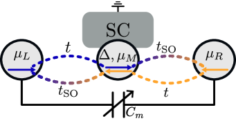
Figure 1: The unit cell of a fermionic quantum computer. Two singly-occupied spin-(anti)polarized quantum dots host the local fermionic modes $L$ and $R$. Two tunnel barriers enable normal $t$ and spin-dependent $t_{SO}$ tunnelings between the two dots. A middle superconducting island mediates superconducting correlations between the two local fermionic modes. An external mutual capacitor $C_{m}$ allows Coulomb interactions between the sites.

Bravyi and Kitaev [1] showed that fermionic quantum computation is equivalent to parity-preserving qubit operations. As a consequence, given a set of fermionic creation ($c^{\dagger}_{i}$) and annihilation operators ($c_{i}$), it follows that

$$\left\{\begin{array}[]{c}\mathcal{U}_{1}(\alpha)=\exp\left(i\alpha c^{\dagger}_{i}c_{i}\right)~{},\quad\mathcal{U}_{2}(\beta)=\exp\left[i\beta\left(c^{\dagger}_{i}c_{j}+c^{\dagger}_{j}c_{i}\right)\right]~{},\\[8.0pt] \mathcal{U}_{3}(\gamma)=\exp\left[i\gamma\left(c^{\dagger}_{i}c^{\dagger}_{j}+c_{j}c_{i}\right)\right]~{},\quad\mathcal{U}_{4}(\delta)=\exp\left(i\delta c^{\dagger}_{i}c_{i}c^{\dagger}_{j}c_{j}\right)\end{array}\right\}$$ (1)

with $\alpha=\beta=\gamma=\pi/4$, and $\delta=\pi$, is a universal set of gate operators. The case of two LFMs is similar to two uncoupled qubits: each operation within a given fermion parity sector is a rotation within $\mathrm{SU}(2)$. In the odd fermion parity sector, the operations $\mathcal{U}_{1}(\alpha)$ and $\mathcal{U}_{2}(\beta)$ are rotations around perpendicular axes in the Bloch sphere. Likewise $\mathcal{U}_{3}(\gamma)$ and $\mathcal{U}_{1}(\delta)$ are perpendicular rotations within the even fermion parity sector. In the presence of an extra ancilla LFM, applying $\mathcal{U}_{4}$ entangles the even and odd subspaces of the two computational LFMs.

Gates processes have a simple physical interpretation within the spin-polarized quantum dots platform

We thus propose a device where excitations occupy single-orbital sites, numbered by the subindex $i$ and $j$. A practical platform for such a proposal is an array of spin-polarized quantum dots, as the scheme shown in Fig. 1. Within this platform, the unitary operations in Eq. 1 are a time-evolution of the following processes:

1. $c^{\dagger}_{i}c_{i}$ onsite energy shift of the fermionic state at site $i$;

2. $c^{\dagger}_{i}c_{j}$ hopping of a fermion between sites $i$ and $j$;

3. $c^{\dagger}_{i}c^{\dagger}_{j}$ superconducting pairing between fermions at sites $i$ and $j$;

4. $c^{\dagger}_{i}c_{i}c^{\dagger}_{j}c_{j}$ Coulomb interaction between fermions at sites $i$ and $j$.

Plunger and tunnel gates control the onsite and hopping processes in quantum dots

We control the onsite energies $\mu_{i}$ with plunger gates. Similarly, a tunnel gate between neighboring pairs of quantum dots controls hopping strength $t$ between them. Manipulation with plunger and tunnel gates is a well-established technique in charge [21, 22] and spin [6] qubits.

We generate pairing between two quantum dots by using a Cooper pair splitter

To implement the superconducting coupling between the spin-polarized dots, we utilize the design of a triplet Copper pair splitter [16, 17, 18, 19, 20]. We include an auxiliary quantum dot in proximity to an s-wave superconductor mediating crossed Andreev reflection (CAR) and elastic cotunelling (ECT) between the two quantum dots that encode the LFMs. Thus, the ECT rate $\Gamma$ sets the hopping strength between the two dots, whereas the CAR rate $\Lambda$ sets the effective superconducting pairing. Because the dots are spin-polarised, the superconducting pairing must be of spin-triplet, enabled by spin-orbit hopping in the hosting material. We quantify the spin-orbit coupling in the hosting material by the spin precession angle between the dots $\theta_{i}=2\pi d/l_{so}$, where $d$ is the interdot distance and $l_{so}$ is the spin-orbit length. The spin-orbit coupling in InSb wires leads to a spin-precession length $l_{\textrm{so}}\approx$100\text{\,}\mathrm{nm}$$ [23, 24] resulting on non-negligible $\theta_{i}$ within the order of dot-to-dot distance.

Capacitive coupling between two quantum dots defines the interaction between LFMs

Finally, we achieve Coulomb interaction between a pair of dots through capacitive coupling $C_{m}$. Our design requires a variable capacitive coupling to implement the $\mathcal{U}_{4}$ gate. Several recent works demonstrate variable capacitive coupling in various platforms: gate-tunable two-dimensional electron gas [25], varactor diodes [26], and external double quantum dots [27].

The three-site device defines the unit cell of the LFM quantum computer

We show the unit cell of a fermionic quantum computer with two LFMs in Fig. 1. The basic building block consists of three tunnel-coupled quantum dots in a material with large spin-orbit coupling. The middle dot is proximitized by an $s$-wave superconductor with an induced gap $\Delta$ that mediates CAR and ECT between the outer dots. The spin-polarised outer dots ($L,R$) encode the LFMs, whereas the middle one is an auxiliary component. Finally, a tunable capacitor couples the outer dots. We generalize the device to an arbitrary number of LFMs by repeating the unit cell in a chain. To read out the fermionic state, we propose to measure the occupation in each quantum dot through charge sensing [28].

3 Effective Hamiltonian

3.1 Tunnel coupling

We consider the limit of spin-polarised quantum dots.

In the absence of capacitive and tunnel coupling, the approximate Hamiltonian for the two spin-polarised dots is

$$H_{d}=\sum_{i=L,R}\mu_{i}c^{\dagger}_{i\sigma_{i}}c_{i\sigma_{i}}~{},$$ (2)

where $c_{i\sigma}$ is the electron anihilation operator at site $i$ and spin $\sigma$, and $\mu_{i}$ is the corresponding chemical potential. The Hamiltonian in Eq. (2) is valid if the charging energy and Zeeman splitting on each dot are larger than all other energy scales in the problem. Recent experiments on similar devices measure charging energy of $2\text{\,}\mathrm{meV}$ and Zeeman splitting of $400\text{\,}\mathrm{\SIUnitSymbolMicro eV}$ at $200\text{\,}\mathrm{mT}$ [16, 17, 19, 20]. Both charging energy and Zeeman splitting are larger than the usual induced superconducting gap inside the quantum dot $\Delta\sim$100\text{\,}\mathrm{\SIUnitSymbolMicro eV}$$ [20, 29, 30], justifying the approximation in Eq. (2).

The middle quantum dot is proximitized by a superconductor.

The proximity of the middle dot to the superconductor suppresses its $g$-factor [31]. Thus, differently from the outer dots, we consider a finite Zeeman energy $B$. The Hamiltonian of the middle dot is

$$H_{\text{ABS}}=\sum_{\sigma,\sigma^{\prime}}\left[\mu_{M}(\sigma_{0})_{\sigma\sigma^{\prime}}+B(\sigma_{z})_{\sigma\sigma^{\prime}}\right]c_{M\sigma}^{\dagger}c_{M\sigma^{\prime}}+\Delta c^{\dagger}_{M\uparrow}c^{\dagger}_{M\downarrow}+\text{h.c.}$$ (3)

where $c_{M\sigma}^{\dagger}$ is the creation operator of electron on the middle dot with spin $\sigma$, $\Delta$ is the induced superconducting gap, and $\sigma_{l}$ are the Pauli matrices ($l=\{0,x,y,z\}$) acting on the spin subspace.

The dots are connected by normal and spin-orbit hoppings.

Both spin-polarised dots in Eq. (2) connect to the middle dot by symmetric tunnel barriers with strength $t$. The barrier $t$ controls both normal and spin-orbit tunneling processes:

$$H_{t}=t\sum_{i=L,R}\cos\theta_{i}c_{i\sigma_{i}}^{\dagger}c_{M\sigma}+it\sum_{i=L,R}\sum_{\sigma^{\prime}}(\sigma_{y})_{\sigma_{i}\sigma^{\prime}}\sin\theta_{i}c_{i\sigma_{i}}^{\dagger}{c_{M\sigma^{\prime}}}+\text{h.c.}~{},$$ (4)

where $\theta_{i}$ is the spin precession angle from dot $i$ to the middle island. Thus, the total Hamiltonian is

$$H=H_{d}+H_{\text{ABS}}+H_{t}~{}.$$ (5)

We treat doubly-occupied states in the middle quantum dot perturbatively.

We obtain the effective low-energy Hamiltonian in the weak-coupling limit, $t\ll\Delta$, through a Schrieffer-Wolf (the derivation is in Appendix A) [32, 33]:

$$\tilde{H}=\sum_{i}\epsilon_{i}^{\sigma_{i}\sigma_{j}}c_{i\sigma_{i}}^{\dagger}c_{i\sigma_{i}}+\sum_{i,j}\Gamma_{\sigma_{i}\sigma_{j}}c^{\dagger}_{i\sigma_{i}}c_{j\sigma_{j}}+\Lambda_{\sigma_{i}\sigma_{j}}c^{\dagger}_{i\sigma_{i}}c^{\dagger}_{j\sigma_{j}}+\text{h.c.}~{},$$ (6)

where $\epsilon_{i}^{\sigma_{i}\sigma_{j}}$ is the renormalised onsite energy of dot $i$, $\Gamma_{\sigma_{i}\sigma_{j}}$ is the ECT rate and $\Lambda_{\sigma_{i}\sigma_{j}}$ is the CAR rate. While $t\neq 0$, we do not vary the chemical potential of the outer dots, $\mu_{L}=\mu_{R}=0$. For simplicity, we also assume no Zeeman splitting within the middle dot $B=0$ and that the spin precession angles are symmetric $\theta_{L}=\theta_{R}=\theta$ (see Appendix A for more general form). In such case, the effective parameters for the anti-parallel spin configuration are:

$$\Lambda_{\uparrow\downarrow}=\kappa\Delta\cos(2\theta)~{},\quad\Gamma_{\uparrow\downarrow}=-i\kappa\mu_{M}\sin{\left(2\theta\right)}~{},$$ (7)

and for the parallel channel:

$$\Lambda_{\uparrow\uparrow}=-i\kappa\Delta\sin{\left(2\theta\right)}~{},\quad\Gamma_{\uparrow\uparrow}=-\kappa\mu_{M}\cos{\left(2\theta\right)}~{},$$ (8)

where

$$\kappa=t^{2}/(\Delta^{2}+\mu_{M}^{2}-B^{2})~{}.$$ (9)

Both onsite corrections terms are equal:

$$\epsilon_{L}^{\sigma_{i}\sigma_{j}}=\epsilon_{R}^{\sigma_{i}\sigma_{j}}=\kappa\mu_{M}.$$ (10)

We observe that the magnitude of $\Lambda_{\sigma_{i}\sigma_{j}}$ is maximum at $\mu_{M}=0$ and drops with increasing chemical potential $\mu_{M}$. On the other hand, $\Gamma_{\sigma_{i}\sigma_{j}}$ has maxima at finite $\mu_{M}$. The magnitude of both processes depends on the spin-precession angle $\theta$ and spin configuration of the outer dots as shown in Fig. 2 (a) and (b). To ensure that operation times for $\mathcal{U}_{2}$ and $\mathcal{U}_{3}$ are similar, the convenient regime is where $\max\Gamma_{\sigma_{i}\sigma_{j}}\sim\max\Lambda_{\sigma_{i}\sigma_{j}}$.

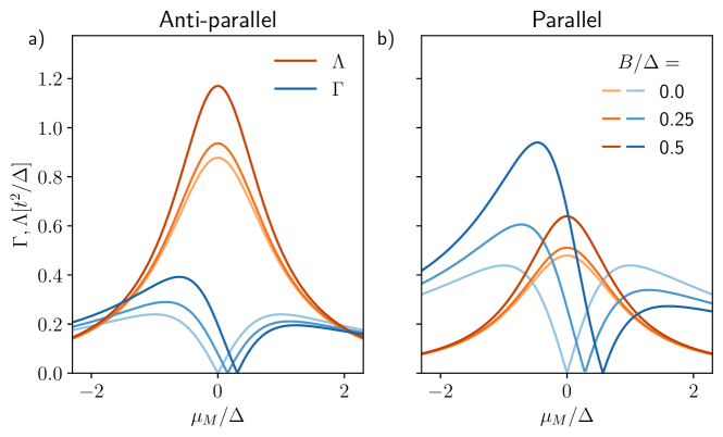
Figure 2: Absolute value of $\Lambda$ (blue) and $\Gamma$ (orange) as a function of $\mu_{M}$ for different values of $B$ for the anti-parallel configuration (a) and the parallel configuration (b). System parameters are $t=0.15$, $\theta_{L}=0.7$ and $\theta_{R}=0.3$.

3.2 Capacitive coupling

The tunable capacitor mediates the Coulomb interaction between the dots.

The electrostatic energy between the two dots is [34]:

$$H_{C}=\sum_{i=L,R}\upsilon_{i}c_{i\sigma_{i}}^{\dagger}c_{i\sigma_{i}}+U_{m}c_{L\sigma_{L}}^{\dagger}c_{L\sigma_{L}}c_{R\sigma_{R}}^{\dagger}c_{R\sigma_{R}}~{},$$ (11)

where $U_{m}=C_{m}e^{2}/\tilde{C}$ is the mutual interaction between the two dots,

$$\upsilon_{L/R}=\frac{C_{R/L}(2n_{g,L/R}+1)+C_{m}n_{g,R/L}}{2\tilde{C}}$$ (12)

is the renormalization to the onsite energy, $\tilde{C}=C_{L}C_{R}-C_{m}^{2}$, $C_{L}$ and $C_{R}$ are the capacitances of the left and right dots, $C_{m}$ is the mutual capacitance, and $n_{g,i}$ is the charge offset in the site $i$. Notice that we consider singly-occupied dots in (11). This approximation is valid when $U_{m}\ll\Delta\ll e^{2}C_{L/R}/\tilde{C}$ because the charging energy renormalization due to the mutual capacitance is negligible in this regime. The last term in (11) gives the Coulomb interaction between the dots required to implement $\mathcal{U}_{4}$.

4 Fermionic quantum gates

4.1 Unitary gate operations

We switch the system parameters on and off to implement operations.

To achieve the fermionic quantum operations defined in Eq. (1), we need to engineer specific time-dependent profiles for the tunable system parameters. In this case, we control the following system parameters through Eqs. (11) and (6): left and right plunger gates ($\mu_{L},\mu_{R}$), middle plunger gate ($\mu_{M}$), tunnel gates ($t$, we treat the two tunnel gates together), and mutual capacitance ($C_{m}$). For simplicity, we only consider square pulses in time

$$H(\tau)=H_{P}(S)[\Theta(\tau)-\Theta(\tau-\tau_{P})]$$ (13)

where $\Theta(\tau)$ is the Heaviside step function, $\tau$ is time and $\tau_{P}$ is the duration of the pulse. We define the pulse Hamiltonian $H_{P}(S)$ as a constant total Hamiltonian where $S=\left\{t,\mu_{M},...\right\}$ are non-zero system parameters in the pulse. For example, $H_{P}(\{t\})$ is a constant Hamiltonian with all system parameters zero except the tunnel coupling $t$. We set the idle (reference) Hamiltonian to one where all gates are zero, $t=\mu_{L}=\mu_{R}=\mu_{M}=U=0$. Thus, the time-evolution operator simplifies to

$$\mathcal{U}(\tau_{2},\tau_{1})=\exp\left[-\frac{i}{\hbar}\int_{\tau_{1}}^{\tau_{2}}d\tau^{\prime}~{}H(\tau^{\prime})\right]=\exp\left[-\frac{i}{\hbar}H_{P}(S)\tau_{P}\right]~{}.$$ (14)

where $\tau_{2},\tau_{1}$ are the initial and final times, and $\tau_{P}$ is the duration of the pulse. In practice, the transition between the idle Hamiltonian and $H_{P}$ in Eq. (13) is not instantaneous but ramps up smoothly over a time $\tau_{R}$ to minimize non-adiabatic transitions.

We design a minimal pulse sequence scheme that implements the universal LFM operations at $B=0$

We engineer the unitary operations as an ordered sequence of pulses defined in Eq. (14). For simplicity, we assume no Zeeman splitting in the middle dot, $B=0$, and leave the discussion of the more general case to section 4.2. In this case, the minimal pulse sequence scheme which implements the gates in Eq. (1) is:

1. onsite operation:

   $$\mathcal{U}_{1}=\exp\left[-\frac{i}{\hbar}H_{P}\left(\{\mu_{L},\mu_{R}\}\right)\tau_{P}\right]~{};$$ (15)

2. hopping operation:

   $$\begin{aligned} \mathcal{U}_{2}&=\exp\left[-\frac{i}{\hbar}H_{P}\left(\{\mu_{L}=\mu,\mu_{R}=\mu\}\right)\tau_{P}^{(4)}\right]\times\exp\left[-\frac{i}{\hbar}H_{P}\left(\{t\}\right)\tau_{P}^{(3)}\right]\\ &\times\exp\left[-\frac{i}{\hbar}H_{P}\left(\{\mu_{L}=\mu,\mu_{R}=\mu\}\right)\tau_{P}^{(2)}\right]\times\exp\left[-\frac{i}{\hbar}H_{P}\left(\{t,\mu_{M}\}\right)\tau_{P}^{(1)}\right]\end{aligned}$$ (16)

3. superconducting pairing operation:

   $$\mathcal{U}_{3}=\exp\left[-\frac{i}{\hbar}H_{P}\left(\{t\}\right)\tau_{P}\right]~{};$$ (17)

4. Coulomb interaction operation:

   $$\mathcal{U}_{4}=\exp\left[-\frac{i}{\hbar}H_{P}\left(\{\mu_{L},\mu_{R}\}\right)\tau_{P}^{(2)}\right]\times\exp\left[-\frac{i}{\hbar}H_{P}\left(\{U\}\right)\tau_{P}^{(1)}\right]~{};$$ (18)

where we indicate as $\tau_{P}^{(i)}$ the duration of the $i$-th pulse.

Some gates require a single pulse because there is no renormalization of other parameters.

In the above scheme, the operations $\mathcal{U}_{1}$ and $\mathcal{U}_{3}$ require a single pulse. The gate $\mathcal{U}_{1}$ requires a single pulse because the dots are uncoupled from one another and the plunger gates affect the onsite energies without inducing any sort of coupling between the dots. Similarly, $\mathcal{U}_{3}$ is also a single operation because the CAR rate is maximum at $\mu_{M}=0$ whereas both ECT rate and onsite corrections are zero according to Eqs. (7— 10). We show the time-dependent simulation of the $\mathcal{U}_{3}$ gate in Fig. 3.

The pulses that lead to unwanted renormalizations require correction gates.

On the other hand, the first pulse of Eq. (16) introduces finite onsite corrections to the outer dots and CAR according to Eqs. (7— 10). Since the onsite corrections are equal, only a global phase factor is accumulated within the odd fermion parity sector. On the other hand, both onsite corrections and CAR result in undesired rotations within the even fermion parity subspace. We undo these operations with an Euler rotation using two orthogonal operations, resulting in the three subsequent pulses in Eq. (16). Similarly, the Coulomb operation in Eq. (18) also requires a correction puls with the plunger gates because the mutual capacitance $C_{m}$ renormalizes the onsite energies in the outer dots, as shown in Eq. (11).

4.2 Finite Zeeman splitting in the middle dot

Zeeman field makes the Hamiltonian asymmetric.

The presence of Zeeman splitting in the middle dot $B$ introduces (see Appendix A) an asymmetric the onsite renormalisation $\epsilon_{L}^{\sigma_{i}\sigma_{j}}\neq\epsilon_{R}^{\sigma_{i}\sigma_{j}}$ and a shift in the minima of $\Gamma_{\sigma_{i}\sigma_{j}}$ shifts away from $\mu_{M}=0$, as shown in Fig. 2. These changes affect the prescriptions for $\mathcal{U}_{2}$ and $\mathcal{U}_{3}$ since these operations require finite $t$.

Applied operations becomes non-orthogonal to $\mathcal{U}_{1}$.

The asymmetric onsite corrections break the orthogonality between $\mathcal{U}_{1}$ and the unitary operation prescribed in Eq. (16). It is still possible to implement the $\mathcal{U}_{2}$ with two non-orthogonal rotation axes in the odd fermion parity sector with additional operations to compensate for the non-orthogonality [35].

Zeeman field and spin-orbit asymmetry induce a finite ECT while applying a CAR operation.

The operation in Eq. (17) also introduces finite $\Gamma_{\sigma_{i}\sigma_{j}}$ in the odd parity sector. We show in Appendix B that anti-parallel spin configuration with symmetric spin-orbit precession $\theta_{L}=\theta_{R}$ removes the shifting $\Lambda$ minima away from $\mu_{M}=0$ and restores the orthogonality of the operations within the even parity sector.

4.3 Gate performance

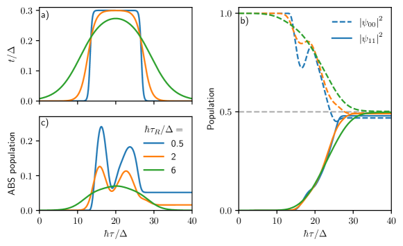
Figure 3: Time-dependent simulation of pairing gate $\mathcal{U}_{3}$ acting on an initial vacuum state with different pulse rise time $\tau_{R}$ profiles. The vacuum population is $\left|\psi_{00}\right|^{2}$ whereas the double occupation population (with middle dot unoccupied) is $\left|\psi_{11}\right|^{2}$. Longer pulses (a) result in a smoother transient population profile (b) and less leakage into the middle ABS state (c). The configuration is the spin-antiparallel with finite Zeeman field within the middle dot $B/\Delta=0.2$ and symmetric spin-orbit precession $\theta_{L}=\theta_{R}=\pi/8$

Short pulse rise times induce transitions outside LFM dots

Switching on the pulse in Eq. (13) happens over a finite rise time $\tau_{R}$. Short rise times $\tau_{R}$ induce transitions from the LFM dots into the middle ABS at energy $\sim\Delta$ which limits the performance of the gates. To avoid such transitions, the pulse times need to be $\tau_{R}\gg\hbar/\Delta$. In Fig. 2 we show the time-dependent simulation of the gate $\mathcal{U}_{3}$ with different rise times. We find that rise times $\tau_{R}>2\hbar/\Delta$ ensures negligible transitions into the ABS. In a system of $\Delta=$100\text{\,}\mathrm{\SIUnitSymbolMicro eV}$$ that corresponds to rise times of $\tau_{R}>$13\text{\,}\mathrm{ps}$$.

Residual capacitance decoheres the device

Current tunable capacitors [25, 26] vary over a limited range. The upper limit for the ratio between the maximum and minimum capacitance $r=C_{\textrm{off}}/C_{\textrm{on}}$ is $r\approx 40$ [25, 26]. Thus, there is a non-negligible residual capacitance between the dots when the $\mathcal{U}_{4}$ gate is off. This residual capacitance acts as an unwanted source of phase and limits the performance of the device. Because such error is coherent, we argue it is possible to offset it after each or a few operations with a compensating $\mathcal{U}_{4}$ pulse. However, since $[\mathcal{U}_{3},\mathcal{U}_{4}]\neq 0$, the $\mathcal{U}_{3}$ operation would require similar compensation pulses to Eq. (16) to offset the effect of the residual capacitor.

5 Future directions

Charge noise is likely the key limiting factor of the device.

Although the device we proposed has the ingredients to implement universal fermionic gates, further work is required to mitigate the main sources of errors. Because of its similarities to a quantum dot charge qubit, we expect the limiting decoherence mechanism to be the same - charge noise [36]. Typical coherence times are on the order of a few nanoseconds [36, 21, 37, 38]. In comparison, Dvir et al. [20] reports CAR/ECT strengths of $\hbar/\Gamma_{\textrm{CAR/ECT}}\approx$10\text{\,}\mathrm{\SIUnitSymbolMicro s}$$ from which we estimate the gate pulse of our proposed device to be $\approx$50\text{\,}\mathrm{ps}$$. On the other hand, if the outer dots in the device shown in Fig. 1 are also proximitized by a superconductor, the local fermionic modes would be encoded by Andreev quasiparticles. Because Andreev states are linear combinations of electron and hole-like excitations, it is possible to design a device that operates with neutral fermions. A similar idea was recently proposed to avoid charge noise in fermion-parity qubits [39]. Finally, minimization of the main sources of errors allows implementation of error-correction codes for fermionic systems [40].

Control of induced superconductive gap would simplify the hopping operation

In the current device, superconducting pairing persists under all possible parameters. Because of that, the hopping operation in Eq. (16) requires a complicated procedure in order to remove the effects of the induced superconducting gap. To simplify the hopping operation, we suggest using a device that allows control of the amount of induced superconducting pairing into the middle dot. For example, a tunnel barrier between the middle dot and the superconducting lead would mediate the induced superconducting pairing. Alternatively, connecting the middle dot to two superconducting leads and controlling the phase difference between them would also allow to control the induced superconducting pairing.

Our device has limited geometry.

Our proposed device consists of a chain of single-orbital fermionic sites. The device layout is a limiting factor, as it only allows nearest-neighbor hoppings, superconducting pairing, and electrostatic interactions. The layout limitations are detrimental to effective scalability. Thus, future works could for example generalize the model to, for example, two-dimensional lattices.

Our device is a ready-to-use static simulator of one-dimensional Hamiltonians with nn interactions.

We showed that the proposed device is a building block of a fermionic quantum computer. However, we must also emphasize that the high control of the system parameters allows to use the same device as a quantum simulator. For example, a chain-like device with the unit cell shown in Fig. 1 at finite $\Gamma$ and $U$ can be directly mapped to the Heisenberg model. Thus, together with superconducting correlations, these devices would be an extension of other quantum dot platforms [41].

Another way to get the interdot Coulomb interaction is with a floating superconducting island.

We mentioned in Sec. 4 that all tunable capacitors proposed present a residual mutual capacitance $C_{\mathrm{off}}$. The external capacitor is necessary because direct mutual capacitance is suppressed by the charge screening in the superconducting island. On the other hand, a floating superconducting island offers a direct interdot capacitance [42]. In a device with a switch between a floating and grounded superconductor, there would be direct control of the mutual capacitance. Moreover, the large charge screening due to the grounded superconducting island sets $C_{\mathrm{off}}\approx 0$, removing the need to fix offset phases due to the residual capacitance.

6 Summary

We showed that Copper pair-splitting devices with tunable capacitors make up a building block of a fermionic quantum computer. We derived the low-energy Hamiltonian and showed that it contains all the necessary processes to build a universal set of gate operations. Moreover, we showed how to use experimentally controllable parameters to implement the gate operations. We find that the presence of Zeeman splitting in the superconducting island complicates the implementation of gates and necessitates additional steps. Based on the low-energy theory, we also studied optimal regimes for the device operation. While our design was mostly inspired by recent experiments, we also discussed how to avoid foreseeable limitations such as (i) the use of neutral fermions to suppress charge noise; (ii) a floating superconducting island to simplify the layout; (iii) control of the superconducting gap to simplify gate operations.

Appendix A Schieffer-Wolff transformation

We rewrite the middle dot Hamiltonian in Andreev basis.

To obtain the effective Hamiltonian from Eq. (6), we perform a Schieffer-Wolff transformation. We, first, diagonalize the Hamiltonian of the middle dot in Eq. (3):

$$H_{\text{ABS}}=(\epsilon_{\text{ABS}}+B)\gamma_{\uparrow}^{\dagger}\gamma_{\uparrow}+(\epsilon_{\text{ABS}}-B)\gamma_{\downarrow}^{\dagger}\gamma_{\downarrow}~{},$$ (19)

where $\epsilon_{\text{ABS}}=\sqrt{\Delta^{2}+\mu_{M}^{2}}$, $\gamma_{\sigma}$ are the annihillation operators of Andreev quasiparticles

$$\gamma_{\uparrow}^{\dagger}=uc^{\dagger}_{M\uparrow}+vc_{M\downarrow}~{},\quad\gamma_{\downarrow}^{\dagger}=uc^{\dagger}_{M\downarrow}-vc_{M\uparrow}~{},$$ (20)

and $u$ and $v$ are the coherence factors.

Unnocupied states in the middle dot form our low-energy manifold.

We now define the occupation basis for the many-body states as $|n_{L},n_{M},n_{R}\rangle$, where $n_{i}$ corresponds to the occupation number at the site $i$. Notice that for the middle dot, we define the number operator as $\hat{n}_{M\sigma}=\gamma_{M\sigma}^{\dagger}\gamma_{M\sigma}$, whereas in the outer dots $\hat{n}_{i\sigma_{i}}=c_{i\sigma_{i}}^{\dagger}c_{i\sigma_{i}}$. Because we consider $\mu_{L/R},B\ll\Delta$, in the absence of hopping between the dots,

$$\langle n_{L},0,n_{R}|H|n_{L},0,n_{R}\rangle\ll\langle n_{L},n_{M},n_{R}|H|n_{L},n_{M},n_{R}\rangle~{},$$ (21)

for $n_{L/R}\in\{0,1\}$, and $n_{M}>0$. Thus, the states with zero occupation in the middle dot form our low-energy manifold.

When the hopping is small, we can treat it as a perturbation.

Occupied states in the middle dot are separated by an energy $\sim\Delta$ from the low-energy manifold. In the weak coupling limit $t\ll\Delta$, the high-energy subspace only contributes to the low-energy dynamics through virtual processes. Therefore, we use a Schieffer-Wolff transformation to obtain the effective Hamiltonian in the low-energy subspace in Eq. (6). Whenever $\mu_{L}=\mu_{R}=0$, the terms in Eq. (6) for the anti-parallel spin configuration are:

$$\epsilon_{R}^{\uparrow\downarrow} =\kappa\left(-2B\sin^{2}{\left(\theta_{R}\right)}+B+\mu_{M}\right),\quad\epsilon_{L}^{\uparrow\downarrow}=\kappa\left(-2B\cos^{2}{\left(\theta_{L}\right)}+B+\mu_{M}\right),$$ (22)

$$\Lambda_{\uparrow\downarrow}=\kappa\Delta\cos(\theta_{L}+\theta_{R})~{},\quad\Gamma_{\uparrow\downarrow}=-i\kappa\left[\mu_{M}\cos{\left(\theta_{L}+\theta_{R}\right)}-B\sin\left(\theta_{L}-\theta_{R}\right)\right]~{},$$ (23)

and for the parallel configuration:

$$\epsilon_{R}^{\uparrow\uparrow} =\kappa\left(-2B\cos^{2}{\left(\theta_{R}\right)}+B+\mu_{M}\right),\quad\epsilon_{L}^{\uparrow\uparrow}=\kappa\left(-2B\cos^{2}{\left(\theta_{L}\right)}+B+\mu_{M}\right),$$ (24)

$$\Lambda_{\uparrow\uparrow}=-i\kappa\Delta\sin{\left(\theta_{L}+\theta_{R}\right)}~{},\quad\Gamma_{\uparrow\uparrow}=-\kappa\left[\mu_{M}\cos{\left(\theta_{L}+\theta_{R}\right)}-B\cos\left(\theta_{L}-\theta_{R}\right)\right]~{},$$ (25)

where

$$\kappa=t^{2}/(\Delta^{2}+\mu_{M}^{2}-B^{2})~{}.$$ (26)

We write the expressions for the shifts of the minima of ECT.

At finite $B$, the chemical potential $\mu_{M}$ at which $\Gamma_{\sigma_{i}\sigma_{j}}=0$ shifts to:

$$\mu_{\text{shift}}^{\uparrow\downarrow}=\frac{B\sin{\left(\theta_{L}-\theta_{R}\right)}}{\sin{\left(\theta_{L}+\theta_{R}\right)}},\quad\mu_{\text{shift}}^{\uparrow\uparrow}=\frac{B\cos{\left(\theta_{L}-\theta_{R}\right)}}{\cos{\left(\theta_{L}+\theta_{R}\right)}}~{},$$ (27)

for anti-parallel and parallel spin configurations.

Appendix B Convenience of the anti-parallel spin configuration

B.1 Orthogonality with symmetric spin precession

In Eq. (22) for the anti-parallel spin configuration we notice that when the spin precession angles are equal $\theta_{L}=\theta_{R}=\theta$, the double occupation onsite energy $\epsilon_{L}+\epsilon_{R}=0$ is zero at $\mu_{M}=0$ and the ETC minima shifts disappear as shown in Eq. (27). That restores the orthogonality of operations within the even parity sector and thus we express $\mathcal{U}_{3}({\gamma})$ operation as:

$$\mathcal{U}_{3}({\gamma})=\exp\left[-\frac{i}{\hbar}H_{P}\left(\{\mu_{L/R}\}\right)\tau_{P}^{(2)}\right]\times\exp\left[-\frac{i}{\hbar}H_{P}\left(\{t\}\right)\tau_{P}^{(1)}\right]~{},$$ (28)

where we compensate a finite $\epsilon_{L}-\epsilon_{R}$ with an onsite pulse. On the other hand, the hopping operation requires additional operations to compensate for non-orthogonality [35]:

$$\begin{aligned} \mathcal{U}_{2}(\beta)&=\exp\left[-\frac{i}{\hbar}H_{P}\left(\{\mu_{L}=\mu,\mu_{R}=\mu\}\right)\tau_{P}^{(N+4)}\right]\times\exp\left[-\frac{i}{\hbar}H_{P}\left(\{t\}\right)\tau_{P}^{(N+3)}\right]\\ &\times\exp\left[-\frac{i}{\hbar}H_{P}\left(\{\mu_{L}=\mu,\mu_{R}=\mu\}\right)\tau_{P}^{(N+2)}\right]\times\exp\left[-\frac{i}{\hbar}H_{P}\left(\{\mu_{L/R}\}\right)\tau_{P}^{(N+1)}\right]\\ &\times\prod_{j=1}^{N/2}\exp\left[-\frac{i}{\hbar}H_{P}\left(\{t,\mu_{M}\}\right)\tau_{P}^{(2j)}\right]\times\exp\left[-\frac{i}{\hbar}H_{P}\left(\{\mu_{L/R}\}\right)\tau_{P}^{(2j-1)}\right]\end{aligned}$$ (29)

where $N$ is the number of pulses required to correct for the non-orthogonality within the odd parity sector.

B.2 Stability and number of operations

To quantify the degree of linear dependence of the operations, we define the following metric

$$\mathcal{L}_{o}=\sqrt{\frac{\left(\epsilon_{L}-\epsilon_{R}\right)^{2}}{\left(\epsilon_{L}-\epsilon_{R}\right)^{2}+\Gamma^{2}}},$$ (30)

$$\mathcal{L}_{e}=\sqrt{\frac{\left(\epsilon_{L}+\epsilon_{R}\right)^{2}}{\left(\epsilon_{L}+\epsilon_{R}\right)^{2}+\Lambda^{2}}}$$ (31)

for $\mathcal{L}_{e}$ even $\mathcal{L}_{o}$ and odd fermion parity sectors. If $\mathcal{L}_{e/o}=0$, the operations are orthogonal and the scheme outlined in Section 4 is valid. On the other hand, if $\mathcal{L}_{e/o}=1$, it is impossible to generate a universal set of operations. To understand how robust the scheme in Eq. (28) is, we consider small deviations from the perfect spin precession case: $\theta_{L}=\theta$ and $\theta_{R}=\theta+\delta$. In this case, the metric $\mathcal{L}_{e/o}$ reads:

$$\mathcal{L}_{o}=\left[1+\left(\frac{\mu_{M}}{B}\tan{2\theta}\right)^{2}\right]^{-1/2}+O(\delta)~{},$$ (32)

$$\mathcal{L}_{e}=\delta\left(\frac{B}{\Delta}\right)\tan{2\theta}+O(\delta^{2})~{}.$$ (33)

Depending on the linear dependence $\mathcal{L}_{e/o}$ of the hopping and pairing operations, we can estimate the maximal number of pulses required to implement an arbitrary operation [35] within a given fermion parity subspace:

$$\mathcal{N}(\mathcal{L}_{e/o})=\lceil\frac{\pi}{\arccos{(\mathcal{L}_{e/o})}}\rceil+1.$$ (34)

References

- [1] S. B. Bravyi and A. Y. Kitaev, Fermionic quantum computation, Ann. Phys-new. York. 298(1), 210 (2002), 10.1006/aphy.2002.6254.
- [2] M. H. Devoret and R. J. Schoelkopf, Superconducting circuits for quantum information: An outlook, Science 339(6124), 1169 (2013), 10.1126/science.1231930.
- [3] M. Kjaergaard, M. E. Schwartz, J. Braumüller, P. Krantz, J. I.-J. Wang, S. Gustavsson and W. D. Oliver, Superconducting qubits: Current state of play, Annual Review of Condensed Matter Physics 11(1), 369 (2020), 10.1146/annurev-conmatphys-031119-050605.
- [4] C. D. Bruzewicz, J. Chiaverini, R. McConnell and J. M. Sage, Trapped-ion quantum computing: Progress and challenges, Applied Physics Reviews 6(2), 021314 (2019), 10.1063/1.5088164.
- [5] H. Häffner, C. Roos and R. Blatt, Quantum computing with trapped ions, Physics Reports 469(4), 155 (2008), https://doi.org/10.1016/j.physrep.2008.09.003.
- [6] G. Burkard, T. D. Ladd, A. Pan, J. M. Nichol and J. R. Petta, Semiconductor spin qubits, Rev. Mod. Phys. 95, 025003 (2023), 10.1103/RevModPhys.95.025003.
- [7] A. Rahmani, K. J. Sung, H. Putterman, P. Roushan, P. Ghaemi and Z. Jiang, Creating and manipulating a laughlin-type fractional quantum hall state on a quantum computer with linear depth circuits, PRX Quantum 1(2) (2020), 10.1103/prxquantum.1.020309.
- [8] F. Arute, K. Arya, R. Babbush, D. Bacon, J. C. Bardin, R. Barends, A. Bengtsson, S. Boixo, M. Broughton, B. B. Buckley, D. A. Buell, B. Burkett et al., Observation of separated dynamics of charge and spin in the fermi-hubbard model (2020), 2010.07965.
- [9] G. A. Quantum, Collaborators*†, F. Arute, K. Arya, R. Babbush, D. Bacon, J. C. Bardin, R. Barends, S. Boixo, M. Broughton, B. B. Buckley, D. A. Buell et al., Hartree-fock on a superconducting qubit quantum computer, Science 369(6507), 1084 (2020), 10.1126/science.abb9811.
- [10] S. McArdle, S. Endo, A. Aspuru-Guzik, S. C. Benjamin and X. Yuan, Quantum computational chemistry, Rev. Mod. Phys. 92, 015003 (2020), 10.1103/RevModPhys.92.015003.
- [11] J. D. Whitfield, J. Biamonte and A. Aspuru-Guzik, Simulation of electronic structure hamiltonians using quantum computers, Mol. Phys. 109(5), 735 (2011), 10.1080/00268976.2011.552441.
- [12] A. S. Wightman, ed., The Collected Works of Eugene Paul Wigner, Springer Berlin Heidelberg, 10.1007/978-3-662-02781-3 (1993).
- [13] Y. Herasymenko, M. Stroeks, J. Helsen and B. Terhal, Optimizing sparse fermionic hamiltonians, Quantum 7, 1081 (2023), 10.22331/q-2023-08-10-1081.
- [14] M. B. Hastings and R. O'Donnell, Optimizing strongly interacting fermionic hamiltonians, In Proceedings of the 54th Annual ACM SIGACT Symposium on Theory of Computing. ACM, 10.1145/3519935.3519960 (2022).
- [15] M. Leijnse and K. Flensberg, Parity qubits and poor man's majorana bound states in double quantum dots, Phys. Rev. B 86(13) (2012), 10.1103/physrevb.86.134528.
- [16] Q. Wang, S. L. D. ten Haaf, I. Kulesh, D. Xiao, C. Thomas, M. J. Manfra and S. Goswami, Triplet cooper pair splitting in a two-dimensional electron gas (2022), 2211.05763.
- [17] G. Wang, T. Dvir, G. P. Mazur, C.-X. Liu, N. van Loo, S. L. D. ten Haaf, A. Bordin, S. Gazibegovic, G. Badawy, E. P. A. M. Bakkers, M. Wimmer and L. P. Kouwenhoven, Singlet and triplet cooper pair splitting in hybrid superconducting nanowires, Nature 612(7940), 448 (2022), 10.1038/s41586-022-05352-2.
- [18] C.-X. Liu, G. Wang, T. Dvir and M. Wimmer, Tunable superconducting coupling of quantum dots via andreev bound states in semiconductor-superconductor nanowires, Phys. Rev. Lett. 129, 267701 (2022), 10.1103/PhysRevLett.129.267701.
- [19] A. Bordin, G. Wang, C.-X. Liu, S. L. D. ten Haaf, G. P. Mazur, N. van Loo, D. Xu, D. van Driel, F. Zatelli, S. Gazibegovic, G. Badawy, E. P. A. M. Bakkers et al., Controlled crossed andreev reflection and elastic co-tunneling mediated by andreev bound states (2022), 2212.02274.
- [20] T. Dvir, G. Wang, N. van Loo, C.-X. Liu, G. P. Mazur, A. Bordin, S. L. D. ten Haaf, J.-Y. Wang, D. van Driel, F. Zatelli, X. Li, F. K. Malinowski et al., Realization of a minimal kitaev chain in coupled quantum dots, Nature 614(7948), 445 (2023), 10.1038/s41586-022-05585-1.
- [21] D. Kim, D. R. Ward, C. B. Simmons, J. K. Gamble, R. Blume-Kohout, E. Nielsen, D. E. Savage, M. G. Lagally, M. Friesen, S. N. Coppersmith and M. A. Eriksson, Microwave-driven coherent operation of a semiconductor quantum dot charge qubit, Nature Nanotechnology 10(3), 243 (2015), 10.1038/nnano.2014.336.
- [22] J. Gorman, D. G. Hasko and D. A. Williams, Charge-qubit operation of an isolated double quantum dot, Phys. Rev. Lett. 95, 090502 (2005), 10.1103/PhysRevLett.95.090502.
- [23] M. W. A. de Moor, J. D. S. Bommer, D. Xu, G. W. Winkler, A. E. Antipov, A. Bargerbos, G. Wang, N. van Loo, R. L. M. O. het Veld, S. Gazibegovic, D. Car, J. A. Logan et al., Electric field tunable superconductor-semiconductor coupling in majorana nanowires, New J. Phys. 20(10), 103049 (2018), 10.1088/1367-2630/aae61d.
- [24] I. van Weperen, B. Tarasinski, D. Eeltink, V. S. Pribiag, S. R. Plissard, E. P. A. M. Bakkers, L. P. Kouwenhoven and M. Wimmer, Spin-orbit interaction in insb nanowires, Phys. Rev. B 91, 201413 (2015), 10.1103/PhysRevB.91.201413.
- [25] N. Materise, M. C. Dartiailh, W. M. Strickland, J. Shabani and E. Kapit, Tunable capacitor for superconducting qubits using an InAs/InGaAs heterostructure, Quantum Science and Technology 8(4), 045014 (2023), 10.1088/2058-9565/aceb18.
- [26] R. S. Eggli, S. Svab, T. Patlatiuk, D. Trüssel, M. J. Carballido, P. C. Kwon, S. Geyer, A. Li, E. P. A. M. Bakkers, A. V. Kuhlmann and D. M. Zumbühl, Cryogenic hyperabrupt strontium titanate varactors for sensitive reflectometry of quantum dots (2023), 2303.02933.
- [27] A. Hamo, A. Benyamini, I. Shapir, I. Khivrich, J. Waissman, K. Kaasbjerg, Y. Oreg, F. von Oppen and S. Ilani, Electron attraction mediated by coulomb repulsion, Nature 535(7612), 395 (2016), 10.1038/nature18639.
- [28] W. Lu, Z. Ji, L. Pfeiffer, K. W. West and A. J. Rimberg, Real-time detection of electron tunnelling in a quantum dot, Nature 423(6938), 422 (2003), 10.1038/nature01642.
- [29] S. T. Gill, J. Damasco, D. Car, E. P. A. M. Bakkers and N. Mason, Hybrid superconductor-quantum point contact devices using InSb nanowires, Applied Physics Letters 109(23) (2016), 10.1063/1.4971394.
- [30] Önder Gül, H. Zhang, F. K. de Vries, J. van Veen, K. Zuo, V. Mourik, S. Conesa-Boj, M. P. Nowak, D. J. van Woerkom, M. Quintero-Pérez, M. C. Cassidy, A. Geresdi et al., Hard superconducting gap in InSb nanowires, Nano Letters 17(4), 2690 (2017), 10.1021/acs.nanolett.7b00540.
- [31] T. D. Stanescu and S. Das Sarma, Proximity-induced low-energy renormalization in hybrid semiconductor-superconductor majorana structures, Phys. Rev. B 96, 014510 (2017), 10.1103/PhysRevB.96.014510.
- [32] K. Vilkelis, A. Manesco, J. D. Torres Luna, S. Miles, M. Wimmer and A. Akhmerov, Fermionic quantum computation with Cooper pair splitters, 10.5281/zenodo.8279302 (2023).
- [33] I. Araya Day, S. Miles, D. Varjas and A. R. Akhmerov, Pymablock, 10.5281/zenodo.7995684 (2023).
- [34] W. G. van der Wiel, S. De Franceschi, J. M. Elzerman, T. Fujisawa, S. Tarucha and L. P. Kouwenhoven, Electron transport through double quantum dots, Rev. Mod. Phys. 75, 1 (2002), 10.1103/RevModPhys.75.1.
- [35] M. Hamada, The minimum number of rotations about two axes for constructing an arbitrarily fixed rotation, Royal Society Open Science 1(3), 140145 (2014), 10.1098/rsos.140145.
- [36] K. D. Petersson, J. R. Petta, H. Lu and A. C. Gossard, Quantum coherence in a one-electron semiconductor charge qubit, Phys. Rev. Lett. 105, 246804 (2010), 10.1103/PhysRevLett.105.246804.
- [37] B. P. Wuetz, D. D. Esposti, A.-M. J. Zwerver, S. V. Amitonov, M. Botifoll, J. Arbiol, A. Sammak, L. M. K. Vandersypen, M. Russ and G. Scappucci, Reducing charge noise in quantum dots by using thin silicon quantum wells, Nature Communications 14(1) (2023), 10.1038/s41467-023-36951-w.
- [38] J. W. G. van den Berg, S. Nadj-Perge, V. S. Pribiag, S. R. Plissard, E. P. A. M. Bakkers, S. M. Frolov and L. P. Kouwenhoven, Fast spin-orbit qubit in an indium antimonide nanowire, Phys. Rev. Lett. 110, 066806 (2013), 10.1103/PhysRevLett.110.066806.
- [39] M. Geier, R. S. Souto, J. Schulenborg, S. Asaad, M. Leijnse and K. Flensberg, A fermion-parity qubit in a proximitized double quantum dot (2023), 2307.05678.
- [40] S. Vijay and L. Fu, Quantum error correction for complex and majorana fermion qubits (2017), 1703.00459.
- [41] C. van Diepen, T.-K. Hsiao, U. Mukhopadhyay, C. Reichl, W. Wegscheider and L. Vandersypen, Quantum simulation of antiferromagnetic heisenberg chain with gate-defined quantum dots, Physical Review X 11(4) (2021), 10.1103/physrevx.11.041025.
- [42] F. K. Malinowski, R. K. Rupesh, L. Pavešić, Z. Guba, D. de Jong, L. Han, C. G. Prosko, M. Chan, Y. Liu, P. Krogstrup, A. Pályi, R. Žitko et al., Quantum capacitance of a superconducting subgap state in an electrostatically floating dot-island (2022), 2210.01519.