Observation of separated dynamics of charge and spin in the Fermi-Hubbard model

Google AI Quantum and collaborators qzj@google.com smelyan@google.com
Abstract

Strongly correlated quantum systems give rise to many exotic physical phenomena, including high-temperature superconductivity. Simulating these systems on quantum computers may avoid the prohibitively high computational cost incurred in classical approaches. However, systematic errors and decoherence effects presented in current quantum devices make it difficult to achieve this. Here, we simulate the dynamics of the one-dimensional Fermi-Hubbard model using 16 qubits on a digital superconducting quantum processor. We observe separations in the spreading velocities of charge and spin densities in the highly excited regime, a regime that is beyond the conventional quasiparticle picture. To minimize systematic errors, we introduce an accurate gate calibration procedure that is fast enough to capture temporal drifts of the gate parameters. We also employ a sequence of error-mitigation techniques to reduce decoherence effects and residual systematic errors. These procedures allow us to simulate the time evolution of the model faithfully despite having over 600 two-qubit gates in our circuits. Our experiment charts a path to practical quantum simulation of strongly correlated phenomena using available quantum devices.

The deceivingly simple Fermi-Hubbard model has greatly advanced our understanding of superconductivity, superfluidity, and quantum magnetism in correlated materials [lee_doping_2006, imada_metal-insulator_1998]. The model is extremely hard to solve on classical computers in certain regimes, and it is widely used to benchmark numerical methods for strongly correlated systems [simons_collaboration_on_the_many-electron_problem_solutions_2015]. A remarkable property of the one-dimensional (1D) Fermi-Hubbard model is spin-charge separation, i.e., spin and charge excitations travel at different speeds due to interparticle interactions [voit_one-dimensional_1995, jagla_numerical_1993, ulbricht_is_2009]. Signatures of spin-charge separation were observed in solid state systems using angle-resolved photoemission spectroscopy [kim_observation_1996, segovia_observation_1999, kim_distinct_2006] and tunneling spectroscopy [tserkovnyak_interference_2003, auslaender_spin-charge_2005, jompol_probing_2009] as well as in cold-atom systems [salomon_direct_2019, vijayan_time-resolved_2020] using site-resolved quantum gas microscopy [boll_spin-_2016, parsons_site-resolved_2016].

Here, we simulate the dynamics of an 8-site 1D Fermi-Hubbard model on a programmable superconducting quantum processor by suddenly removing the trapping potentials and turning on the on-site interactions. We observe separations in the spreading velocities of spin and charge in a regime beyond the low-energy physics described by the Luttinger liquid theory [haldane_luttinger_1981, imambekov_one-dimensional_2012]. Our platform enjoys the flexibility that analog devices do not, such as the ability to measure arbitrary observables, reverse the time evolution, and prepare for various initial states including BCS-type states [jiang_quantum_2018]. It also has high repetition rates compared to some other platforms and avoids finite temperature effects.

The key technical advancement that enabled this experiment is a calibration protocol that we recently developed for entangling gates, which we call Floquet calibration. It allows for gate parameters to be characterized rapidly and precisely, which unlocks the ability to compensate for systematic errors caused by drifts and fluctuations. Floquet calibration is based on the idea that an entangling gate can be uniquely determined by the eigenvalues of the composite gates consisting of the entangling gate and several different sets of single-qubit gates; one gets different snapshots of the entangling gate by changing the parameters in the single-qubit gates. It is also robust to state preparation and measurement errors, sharing many common traits with robust phase estimation for calibrating single-qubit gates [kimmel_robust_2015, rudinger_experimental_2017]. We also show that decoherence effects can be drastically suppressed by using a combination of error mitigation schemes. Along with our calibration tool, these techniques allow us to increase the circuit depths (evolution times) by an order of magnitude. Our work paves the way toward simulating strongly correlated quantum systems [jordan_quantum_2012, georgescu_quantum_2014, barends_digital_2015, wecker_solving_2015, hensgens_quantum_2017, kivlichan_quantum_2018, jiang_quantum_2018, smith_simulating_2019, chiaro_growth_2019, mcardle_quantum_2020, rahmani_creating_2020, dallaire-demers_application_2020] on existing digital quantum computers.

I The model
Refer to caption
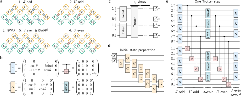
Figure 1: Qubit layouts and quantum circuits. a. The 5 stages in a Trotter step, where the orange and green qubits represent spin-up and -down fermionic sites, respectively. In stage 1 and 2, the blue and red edges represent the hopping and interaction terms, respectively. In stage 3, we change the positions of the odd and even sites by applying the iSWAP gates across the blue edges, which allows for implementing U𝑈U even in the next stage. In stage 5, we swap the sites back to their original positions using the iSWAPsuperscriptiSWAP\mbox{\footnotesize{iSWAP}}^{\dagger} gates, which are combined with the J𝐽J even terms. b. The matrix representations of the two-qubit gates. The Givens rotation gate G𝐺G (yellow) is used to prepare the initial state. The iSWAP-like gate K𝐾K (blue) and the CPHASE gate (red) are used to implement the time evolution under the hopping and interaction terms, respectively. The iSWAP gate (green) is a special case of K(θ)𝐾𝜃K(\theta), with θ=-π/2𝜃𝜋2\theta=\mathord{-}\pi/2. In Supplementary Fig. S1, we show that any of the four gates can be decomposed into two K(π/4)𝐾𝜋4K(\pi/4) gates and several single-qubit gates. c. The entire quantum circuit includes an initialization part, η𝜂\eta Trotter steps, and measurements in the Pauli-Z𝑍Z basis. d. The circuit to prepare the ground state of a noninteracting Hamiltonian with two particles (excitations), where the angles of the Givens rotations can be determined using an efficient classical algorithm. e. The quantum circuit to implement one Trotter step of the model.

Consider the 1D Fermi-Hubbard model on L𝐿L lattice sites with open-boundary conditions,

H𝐻\displaystyle H =Jj=1L1ν=,cj,νcj+1,ν+h.c.formulae-sequenceabsent𝐽superscriptsubscript𝑗1𝐿1subscript𝜈superscriptsubscript𝑐𝑗𝜈subscript𝑐𝑗1𝜈hc\displaystyle=-J\sum_{j=1}^{L-1}\sum_{\nu=\mathord{\uparrow,\hskip 0.4pt\downarrow}}\!c_{j,\nu}^{\dagger}c_{j+1,\nu}+\mathrm{h.c.}
+Uj=1Lnj,nj,+j=1Lν=,ϵj,νnj,ν,𝑈superscriptsubscript𝑗1𝐿subscript𝑛𝑗subscript𝑛𝑗superscriptsubscript𝑗1𝐿subscript𝜈subscriptitalic-ϵ𝑗𝜈subscript𝑛𝑗𝜈\displaystyle\quad+U\sum_{j=1}^{L}n_{j,\uparrow}\hskip 0.4ptn_{j,\downarrow}+\sum_{j=1}^{L}\sum_{\nu=\mathord{\uparrow,\hskip 0.4pt\downarrow}}\epsilon_{j,\nu}\,n_{j,\nu}\,, (1)

where cj,νsubscript𝑐𝑗𝜈c_{j,\nu} (cj,νsuperscriptsubscript𝑐𝑗𝜈c_{j,\nu}^{\dagger}) are the fermionic annihilation (creation) operators associated to site number j𝑗j and spin state ν𝜈\nu, and nj,ν=cj,νcj,νsubscript𝑛𝑗𝜈superscriptsubscript𝑐𝑗𝜈subscript𝑐𝑗𝜈n_{j,\nu}=c_{j,\nu}^{\dagger}c_{j,\nu} are the number operators. The hopping term with coefficient J𝐽J in Eq. (I) describes particles tunneling between neighboring sites, the onsite interaction term with coefficient U𝑈U introduces an energy difference for doubly occupied sites, and the term ϵj,νsubscriptitalic-ϵ𝑗𝜈\epsilon_{j,\nu} represents spin-dependent local potentials. The charge and spin densities are defined as the sum and difference of the spin-up and -down particle densities, respectively,

ρj±=nj,±nj,.superscriptsubscript𝜌𝑗plus-or-minusplus-or-minusdelimited-⟨⟩subscript𝑛𝑗delimited-⟨⟩subscript𝑛𝑗\displaystyle\rho_{j}^{\pm}=\langle\,n_{j,\uparrow}\,\rangle\pm\langle\,n_{j,\downarrow}\,\rangle\,. (2)

We map the fermionic operators to qubit operators using the Jordan-Wigner transformation (JWT) for each spin state, cj,ν12(Xj,ν+iYj,ν)Z1,νZj1,νmaps-tosubscript𝑐𝑗𝜈12subscript𝑋𝑗𝜈𝑖subscript𝑌𝑗𝜈subscript𝑍1𝜈subscript𝑍𝑗1𝜈c_{j,\nu}\;\mapsto\;\frac{1}{2}\,(X_{j,\nu}+iY_{j,\nu})\,Z_{1,\nu}\cdots Z_{j-1,\nu}, where Xj,νsubscript𝑋𝑗𝜈X_{j,\nu}, Yj,νsubscript𝑌𝑗𝜈Y_{j,\nu}, and Zj,νsubscript𝑍𝑗𝜈Z_{j,\nu} are the Pauli operators. Under the JWT, the unoccupied and occupied spin orbitals are represented by the qubit states | 0delimited-|⟩ 0\lvert\,0\,\rangle and | 1delimited-|⟩1\lvert\,1\,\rangle, respectively. We use the product formula [childs_nearly_2019], i.e., Trotter steps, to simulate the time evolution of the system, where each term in the Hamiltonian (I) is implemented separately. A single Trotter step is implemented with the 5 stages depicted in Fig. 1a, where each spin state of the model is mapped to a zigzag chain of 888 qubits; this optimizes the circuit depths under the geometric constraints.

Refer to caption
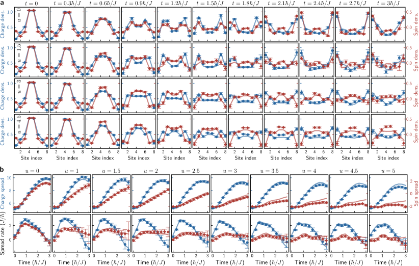
Figure 2: Separation in charge and spin densities. We initialize the quantum state with N=N=2subscript𝑁subscript𝑁2N_{\uparrow}=N_{\downarrow}=2 (quarter filling), where the charge and spin densities ρj±=nj,±nj,superscriptsubscript𝜌𝑗plus-or-minusplus-or-minusdelimited-⟨⟩subscript𝑛𝑗delimited-⟨⟩subscript𝑛𝑗\rho_{j}^{\pm}=\langle\,n_{j,\uparrow}\,\rangle\pm\langle\,n_{j,\downarrow}\,\rangle are peaked around the middle sites. We then evolve the state under the Fermi-Hubbard Hamiltonian (I) with Trotter step length τ=0.3/J𝜏0.3Planck-constant-over-2-pi𝐽\tau=0.3\hskip 0.4pt\hbar/J. Points and solid lines represent experimental and numerical (exact) results, respectively. a. Time evolved charge (blue) and spin (red) densities for uU/J=3𝑢𝑈𝐽3u\equiv U/J=3 with tJ/=0,1.2,1.8,3𝑡𝐽Planck-constant-over-2-pi01.21.83t\hskip 0.4ptJ/\hbar=0,1.2,1.8,3 (corresponding to Trotter numbers η=0,4,6,10𝜂04610\eta=0,4,6,10), where the error bars represent the standard error of the mean over 16 simulations with different choices of qubits and their arrangements, see Supplementary Fig. S9; the uncertainties due to finite sample sizes are much smaller (omitted on the plots). The charge density spreads faster than the spin density and reaches the boundaries earlier. b. The charge and spin spreads κ±=j|j(L+1)/2|ρj±superscript𝜅plus-or-minussubscript𝑗𝑗𝐿12superscriptsubscript𝜌𝑗plus-or-minus\kappa^{\pm}=\sum_{j}\,\big{\lvert}j-(L+1)/2\big{\rvert}\,\rho_{j}^{\pm} as functions of the evolution time. For u=0𝑢0u=0, they almost lay on top of each other; the small discrepancy is due to the parasitic CPHASE in our native gate. In comparison, they are well separated for larger interaction strengths u1𝑢1u\geq 1. c. The numerical derivatives of κ±superscript𝜅plus-or-minus\kappa^{\pm} with respect to the evolution time.

Under the JWT, the hopping term cj,νcj+1,ν+h.c.formulae-sequencesuperscriptsubscript𝑐𝑗𝜈subscript𝑐𝑗1𝜈hcc_{j,\nu}^{\dagger}c_{j+1,\nu}+\mathrm{h.c.} is mapped to 12(Xj,νXj+1,ν+Yj,νYj+1,ν)12subscript𝑋𝑗𝜈subscript𝑋𝑗1𝜈subscript𝑌𝑗𝜈subscript𝑌𝑗1𝜈\frac{1}{2}\hskip 0.4pt(X_{j,\nu}X_{j+1,\nu}+Y_{j,\nu}Y_{j+1,\nu}). Its time evolution can be implemented using the two-qubit gate K(θ)𝐾𝜃K(\theta) in Fig. 1b. This gate is used in the first and last stages in the circuit depicted in Fig. 1e. In the first stage, we set θ=τJ/𝜃𝜏𝐽Planck-constant-over-2-pi\theta=-\tau\hskip 0.4ptJ/\hbar to implement a time step of length τ𝜏\tau. In the last stage, we set θ=τJ/+π/2𝜃𝜏𝐽Planck-constant-over-2-pi𝜋2\theta=-\tau J/\hbar+\pi/2, where the extra angle π/2𝜋2\pi/2 is used to undo the iSWAP gates in the third stage to change the positions of the fermionic sites. The gate K(θ)𝐾𝜃K(\theta) with arbitrary θ𝜃\theta can be decomposed into two K(π/4)=iSWAP𝐾𝜋4superscriptiSWAPK(\pi/4)=\sqrt{\mbox{\footnotesize{iSWAP}}}^{\,{\dagger}} gates and several single-qubit Z𝑍Z rotations, see Supplementary Fig. S1c. Our hardware native two-qubit gate takes the form K(ϑ)CPHASE(φ)𝐾italic-ϑCPHASE𝜑K(\vartheta)\,\mbox{\footnotesize{CPHASE}}\hskip 0.4pt(\varphi), where ϑπ/4italic-ϑ𝜋4\vartheta\approx\pi/4 and the parasitic controlled phase φπ/20less-than-or-similar-to𝜑𝜋20\varphi\lesssim\pi/20. At the time we took the data, the means and standard deviations of the two parameters across different pairs of qubits were ϑ=0.783±0.012 radtimesitalic-ϑplus-or-minus0.7830.012radian\vartheta=0.783\pm 0.012\text{\,}\mathrm{rad} and φ=0.138±0.015 radtimes𝜑plus-or-minus0.1380.015radian\varphi=0.138\pm 0.015\text{\,}\mathrm{rad}. The CPHASE(φ)CPHASE𝜑\mbox{\footnotesize{CPHASE}}\hskip 0.4pt(\varphi) term introduces an interaction term between neighboring fermionic sites Vnj,νnj+1,ν𝑉subscript𝑛𝑗𝜈subscript𝑛𝑗1𝜈Vn_{j,\nu}\,n_{j+1,\nu} with V=2φ/τ𝑉2Planck-constant-over-2-pi𝜑𝜏V=2\hbar\varphi/\tau. It has sizable effects for longer evolution times, and we include it in our numerical simulations to compare to experimental results. The entanglement part in our native two-qubit gate takes about 12 nstimes12nanosecond12\text{\,}\mathrm{ns} and is preceded by single-qubit Z𝑍Z rotations, which take 10 nstimes10nanosecond10\text{\,}\mathrm{ns} with a 5 nstimes5nanosecond5\text{\,}\mathrm{ns} padding on each side. Therefore, one hopping term takes about 2×32 ns=64 ns2times32nanosecondtimes64nanosecond2\times$32\text{\,}\mathrm{ns}$=$64\text{\,}\mathrm{ns}$ to implement on the hardware.

The time evolution of the on-site interaction term nj,nj,subscript𝑛𝑗subscript𝑛𝑗n_{j,\uparrow}\hskip 0.4ptn_{j,\downarrow} can be implemented using CPHASE(ϕ)CPHASEitalic-ϕ\mbox{\footnotesize{CPHASE}}(\phi) gate with ϕ=τU/italic-ϕ𝜏𝑈Planck-constant-over-2-pi\phi=\tau U/\hbar. It can be decomposed exactly into two native two-qubit gates and single-qubit X𝑋X and Z𝑍Z rotations, see Supplementary Information A. There are three layers of X𝑋X rotations (microwave gates) in the composite gate, each taking about 25 nstimes25nanosecond25\text{\,}\mathrm{ns}. Therefore, the entire composite CPHASE gate takes about 139 nstimes139nanosecond139\text{\,}\mathrm{ns} to implement. As shown in Fig. 1a, we implement the CPHASE gate on the odd and even sites separately due to geometry constraints. Idling qubits are susceptible to crosstalk and low-frequency noises in the Z𝑍Z basis, and we mitigate them by applying spin echos consisting of pairs of X𝑋X gates (not shown in Fig. 1).

We initialize the system into the ground state of a non-interacting fermionic Hamiltonian using networks of Givens rotations [wecker_solving_2015], i.e., two-mode fermionic basis transformations. The Givens rotation takes the matrix form G𝐺G in Fig. 1b when acting on neighboring qubits. It can also be decomposed into two K(π/4)𝐾𝜋4K(\pi/4) gates and single-qubit Z𝑍Z rotations, see Supplementary Fig. S1b. By parallelizing the Givens rotations, the ground state of an arbitrary L𝐿L-mode non-interacting Hamiltonian can be prepared in circuit depth 𝒪(L)𝒪𝐿\mathcal{O}(L)  [kivlichan_quantum_2018, jiang_quantum_2018]. Recently, the Givens rotation network was successfully used to variationally construct a chemically-accurate Hartree-Fock state [collaborators_hartree-fock_2020]. Here we use the OpenFermion code [mcclean_openfermion_2020] based on the scheme in [jiang_quantum_2018], which requires L2/4similar-tosuperscript𝐿24\mathord{\sim}L^{2}/4 Givens rotations with circuit depth Lsimilar-to𝐿\mathord{\sim}L near half filling. In Fig. 1d, we plot the initialization circuit for two fermions.

II Separation of spin and charge velocities

In the Luttinger liquid description of the 1D Fermi-Hubbard model [luttinger_exactly_1963, mattis_exact_1965, lieb_absence_1968], low-energy charge and spin excitations propagate at different characteristic velocities; see Supplementary Information B. It is based on the assumption that the system is close to its ground state. Here we observe separations in the dynamics of charge and spin densities in a highly excited regime, where the Luttinger liquid theory does not formally apply.

Consider an 8-site 1D Fermi-Hubbard system with Nνsubscript𝑁𝜈N_{\nu} particles in the spin state ν𝜈\nu. We prepare the initial state |ψ0delimited-|⟩subscript𝜓0\lvert\,\psi_{0}\,\rangle as the ground state of an non-interacting Hamiltonian H0subscript𝐻0H_{0} by setting U=0𝑈0U=0 in Eq. (I). The local potentials in H0subscript𝐻0H_{0} are chosen to have a Gaussian form ϵj,ν=λνe12(jmν)2/σν2subscriptitalic-ϵ𝑗𝜈subscript𝜆𝜈superscript𝑒12superscript𝑗subscript𝑚𝜈2superscriptsubscript𝜎𝜈2\epsilon_{j,\nu}=-\lambda_{\nu}\,e^{-\frac{1}{2}\hskip 0.4pt(j-m_{\nu})^{2}/\sigma_{\nu}^{2}}, where λνsubscript𝜆𝜈\lambda_{\nu}, mνsubscript𝑚𝜈m_{\nu}, and σνsubscript𝜎𝜈\sigma_{\nu} set the magnitude, center, and width of the potentials, respectively. We set the parameters of the spin-up Gaussian potential to λ=4subscript𝜆4\lambda_{\uparrow}=4, m=4.5subscript𝑚4.5m_{\uparrow}=4.5, and σ=1subscript𝜎1\sigma_{\uparrow}=1 while leaving the spin-down potential to zero. This generates initial charge and spin density peaks in the middle of the chain, see subplot t=0𝑡0t=0 in Fig. 2a.

Refer to caption
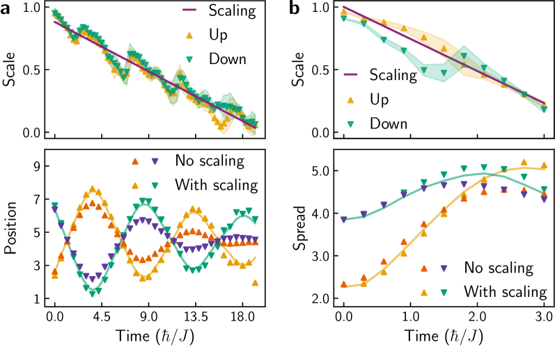
Figure 3: Noninteracting time evolution and error mitigation. a. Time evolution of the particle densities nj,νdelimited-⟨⟩subscript𝑛𝑗𝜈\langle\,n_{j,\hskip 0.4pt\nu}\,\rangle, where j=1,,8𝑗18j=1,\ldots,8 and ν=,𝜈\nu=\uparrow,\downarrow. The experiment results match well with the numerics (exact) for t16.5/Jless-than-or-similar-to𝑡16.5Planck-constant-over-2-pi𝐽t\lesssim 16.5\hskip 0.4pt\hbar/J, corresponding to a circuit depth of 228 layers of two-qubit gates with execution time 7.3 μstimes7.3𝜇s7.3\text{\,}\mu\mathrm{s}. b. Demonstrating error mitigation schemes using the average positions jnj,νjsubscript𝑗delimited-⟨⟩subscript𝑛𝑗𝜈𝑗\sum_{j}\langle\,n_{j,\hskip 0.4pt\nu}\,\rangle\,j, where the solid lines represent numerical results for the spin-up (yellow) and -down (green) particles. The triangles and the shaded areas represent the means and sample standard deviations over 16 simulations with different choices of qubits and their arrangements, see Supplementary Fig. S9. This procedure, which we call qubit assignment averaging, removes inhomogeneous effects in the system. Decoherence due to loss of excitations (T1subscript𝑇1T_{1} errors) can be removed by postselecting the measurement results with the correct numbers of excitations. Floquet calibration improves both the means and standard deviations of the average positions. Crucially, the particle density distributions obtained after the calibration are similar to the exact solutions with damped amplitudes. The damping factor is a function of the evolution time t𝑡t; its value is approximately 111 at t=0𝑡0t=0 and 0.160.160.16 at t=16.5/J𝑡16.5Planck-constant-over-2-pi𝐽t=16.5\hskip 0.4pt\hbar/J. This allows us to get excellent agreement with theory predictions by rescaling.

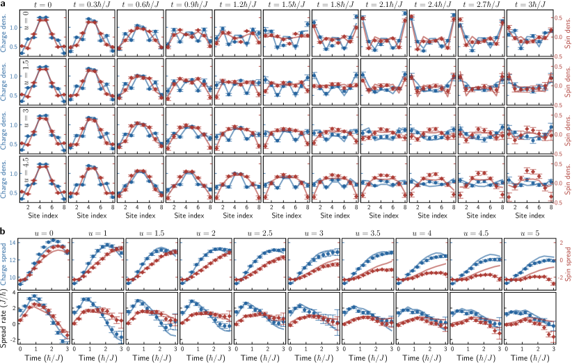
We then evolve the system under the Hamiltonian (I) with the Trotter step described in Fig. 1e by setting the time step length to τ=0.3/J𝜏0.3Planck-constant-over-2-pi𝐽\tau=0.3\hskip 0.4pt\hbar/J and the local potentials to ϵj,ν=0subscriptitalic-ϵ𝑗𝜈0\epsilon_{j,\nu}=0. In Fig. 2a, we plot the distributions of the charge and spin densities at several evolution times for N=N=2subscript𝑁subscript𝑁2N_{\uparrow}=N_{\downarrow}=2 and uU/J=3𝑢𝑈𝐽3u\equiv U/J=3, where the dynamics of the charge and spin degrees of freedom are separated. We leave more detailed results for this case and the N=N=3subscript𝑁subscript𝑁3N_{\uparrow}=N_{\downarrow}=3 case in Supplementary Figs. S12 and S13, respectively.

To quantify the degree that charge and spin densities spread from the middle of the chain, we introduce

κη±=j=1L\scalerel[5pt]|\ensurestackMath\addstackgap[1.5pt]|j(L+1)/2\scalerel[5pt]|\ensurestackMath\addstackgap[1.5pt]|ρj,η±\displaystyle\kappa_{\eta}^{\pm}=\sum_{j=1}^{L}\,\mathopen{\scalerel*[5pt]{\big{\lvert}}{\ensurestackMath{\addstackgap[1.5pt]{\big{\lvert}}}}}j-(L+1)/2\mathclose{\scalerel*[5pt]{\big{\rvert}}{\ensurestackMath{\addstackgap[1.5pt]{\big{\rvert}}}}}\,\rho_{j,\eta}^{\pm}\,

where ρj,η±=nj,±nj,superscriptsubscript𝜌𝑗𝜂plus-or-minusplus-or-minusdelimited-⟨⟩subscript𝑛𝑗delimited-⟨⟩subscript𝑛𝑗\rho_{j,\eta}^{\pm}=\langle\,n_{j,\uparrow}\,\rangle\pm\langle\,n_{j,\downarrow}\,\rangle are the charge and spin densities after η𝜂\eta Trotter steps. In Fig. 2b, we plot κ±superscript𝜅plus-or-minus\kappa^{\pm} as functions of the evolution time for several interaction strengths u𝑢u. When u=0𝑢0u=0, they nearly coincide with each other; the small separation is the result of the nearest-neighbor interaction term Vnj,νnj+1,ν𝑉subscript𝑛𝑗𝜈subscript𝑛𝑗1𝜈Vn_{j,\nu}\,n_{j+1,\nu}, caused by the parasitic CPHASE in our native gate. The gaps between κ+superscript𝜅\kappa^{+} and κsuperscript𝜅\kappa^{-} widen as u𝑢u increases, demonstrating increased separations as the system goes into the strongly interacting regime. The charge spread κ+superscript𝜅\kappa^{+} reaches the maximum value after it has fully hit the boundaries. In comparison, κsuperscript𝜅\kappa^{-} increases at significantly lower rates for all u0𝑢0u\neq 0 and never fully reaches the boundaries within the maximum evolution time.

In Fig. 2c, we plot the numerical derivatives of the charge and spin spreads κ±superscript𝜅plus-or-minus\kappa^{\pm}. Because our initial wavefunction is real, both charge and spin currents equal zero at t=0𝑡0t=0. The small nonzero values of the observed initial rates of charge and spin spreads are due to the finite Trotter step length and the parasitic CPHASE in the initialization circuit. The charge spreading rate gradually increases until the particles starts to hit the boundaries. As the interaction strength u𝑢u increases, the maximum spin spread rate decreases. In comparison, the maximum charge spread rate roughly keeps the same.

III Error mitigation and calibration

To reach the desired circuit depths, we employ a combination of error mitigation and calibration schemes. To illustrate that, we consider the case where there is exactly one particle in each spin state N=N=1subscript𝑁subscript𝑁1N_{\uparrow}=N_{\downarrow}=1. We initialize the spin-up (down) particle into a left (right)-moving Gaussian wavepacket. This can be achieved by first creating a real Gaussian wavepacket with the Givens rotations and then generating a phase gradient using single-qubit Z𝑍Z rotations. We evolve the system under the hopping terms by including only the first and last stages in Fig. 1e with time step length τ=0.3/J𝜏0.3Planck-constant-over-2-pi𝐽\tau=0.3\hbar/J. In Fig. 3a, we compare the numerics with experimental results after applying all the error mitigation schemes. They match well with each other up to t16.5/J𝑡16.5Planck-constant-over-2-pi𝐽t\approx 16.5\hskip 0.4pt\hbar/J (or 555555 Trotter steps), and the clear interference patterns at larger times indicate that the evolution is coherent instead of diffusive. The two spin states evolve independently here, i.e., there is no gate between the corresponding sets of qubits. However, we can account for the effects of crosstalks more properly by including the two spin states. The impact of each step in our error mitigation procedure is illustrated in Fig. 3b, which we describe below one by one.

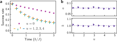
The quantum circuit for the Fermi-Hubbard model conserves the total number of excitations for each spin state. However, excitations can leave the system due to interactions with the environment. In Supplementary Fig. S11, we plot the T1subscript𝑇1T_{1} map of the device at the time that the final data were taken. This kind of error can be removed by postselecting the measurement results with the correct numbers of excitations. It also reduces state preparation and measurement (SPAM) errors to some extent. The postselection success rates of the noninteracting instance shown in Fig. 3 are about 0.50.50.5 for η=0𝜂0\eta=0 and 0.20.20.2 for η=55𝜂55\eta=55, where η𝜂\eta is the number of Trotter steps. In Fig. 4a, we plot the success rates as functions of the evolution time. We take 20,000 samples for each circuit to make sure that the uncertainties of the expectation values are low after postselection.
Refer to caption
Figure 4: Postselection success rate and rescaling parameters. a. The post selection success rates as functions of the evolution time. The squares denote the results for the noninteracting case in Fig. 3, which decays much slower due to the reduced number of gates in each Trotter step. The horizontal and vertical bars denote results for the interacting case in Fig. 2 with different values of u𝑢u; the cross formation of the horizontal and vertical bars shows that the success rate does not depend on u𝑢u. b. The rescaling parameters a𝑎a and b𝑏b in Eq. (3) for the case in Fig. 2. Their values barely depend on the interaction strength u𝑢u, allowing one to infer them by comparing numerical and experimental results in the weakly interacting regime.

Systematic errors are especially detrimental to quantum computation as their effects can add up coherently. In addition to our routine calibration, we also use Floquet calibration, a fast calibration method that we recently developed for characterization of entangling gates. To capture crosstalks, we calibrate the two-qubit gates in each configuration in Fig. 1a by applying them simultaneously; the results are then used to correct the two-qubit gates in the quantum circuit within the same configuration. Floquet calibration can determine most parameters of the two-qubit gates to an uncertainty of less than 103 radtimesE-3radian{10}^{-3}\text{\,}\mathrm{rad} under one minute, sufficiently fast to characterize errors due to drifts and fluctuations in the control fields and qubit frequencies. It is also robust to state preparation and measurement (SPAM) errors in general. In Supplementary Fig. S2, we plot the parameters in our native two-qubit gate obtained using Floquet calibration during a period of several hours. We also plot the two-qubit gate fidelity map from our routine calibration using cross-entropy benchmarking (XEB) in Supplementary Fig. S11; more about XEB and our calibration process can be found in Supplementary Information in Ref. [arute_quantum_2019]. We leave detailed discussions on the implementations and properties of Floquet calibration in Supplementary Information C.

Inhomogeneities in gate parameters and decoherence rates are common in quantum computing devices. They make the experiment results unpredictable and implementation dependent. We solve this issue using qubit assignment averaging, where experiment results are averaged over 16 different realizations, see Supplementary Fig. S9. In each realization, we either choose a different set of qubits, arrange the qubits differently, or do both. In Fig. 3b, we show that the averaged results are smooth even if the outcomes from individual implementations fluctuate significantly. More importantly, averaging makes it possible to describe the simulation results using models with randomized parameters. The values of the observables are often damped in a predictable way in these models, making it possible for further mitigation of the errors.

Finally, we rescale the damped expectation values nj,νdelimited-⟨⟩subscript𝑛𝑗𝜈\langle\,n_{j,\nu}\,\rangle, leading to excellent agreement with theoretical predictions. We choose the fiducial point for rescaling to be n¯ν=Nν/Lsubscript¯𝑛𝜈subscript𝑁𝜈𝐿\bar{n}_{\nu}=N_{\nu}/L, i.e., the averaged particle density for the spin state ν𝜈\nu. We observe that the damping factor is approximately linear in the number of Trotter steps η𝜂\eta,

nj,νexpn¯νnj,νnumn¯νbaη,subscriptdelimited-⟨⟩subscript𝑛𝑗𝜈expsubscript¯𝑛𝜈subscriptdelimited-⟨⟩subscript𝑛𝑗𝜈numsubscript¯𝑛𝜈𝑏𝑎𝜂\displaystyle\frac{\langle\,n_{j,\nu}\,\rangle_{\mathrm{exp}}-\bar{n}_{\nu}}{\langle\,n_{j,\nu}\,\rangle_{\mathrm{num}}-\bar{n}_{\nu}}\approx b-a\eta\,, (3)

where exp and num stand for experimental and numerical results, respectively. The parameter a𝑎a (b𝑏b) describes the damping effect of the Trotter steps (initial state preparation circuit). The linear relation fits the experimental results well when the damping factor is 0.2greater-than-or-equivalent-toabsent0.2\gtrsim 0.2 for both noninteracting and interacting cases, see Supplementary Fig. S9. The fitted values of a𝑎a and b𝑏b hardly depend on the interaction strength U𝑈U, see Fig. 4b. Therefore, we can estimate their values by comparing the experimental and numeric results in a regime that is easy to solve classically, e.g., the weak interaction regime. The linear relation (3) is not essential to our rescaling procedure. However, the weak dependence of the damping factor on the interaction strength U𝑈U is crucial.

Case
tevolsubscript𝑡evolt_{\mathrm{evol}} (/JPlanck-constant-over-2-pi𝐽\hbar/J) tcircuitsubscript𝑡circuitt_{\mathrm{circuit}} (μs𝜇s\mu\mathrm{s}) Circuit depths 2-qubit counts μ𝜇\mu-wave counts RZsubscript𝑅𝑍R_{Z} counts
U0𝑈0U\neq 0 NP=4,6subscript𝑁𝑃46N_{P}=4,6
1.5 2.8 159 328 364 566
3.0 5.2 289 608 724 1056
U=0𝑈0U=0 NP=2subscript𝑁𝑃2N_{P}=2
9.0 4.1 257 434×2434absent2434\scalebox{1.0}{$\times 2$} 2 836×2836absent2836\scalebox{1.0}{$\times 2$}
16.5 7.3 457 784×2784absent2784\scalebox{1.0}{$\times 2$} 2 1511×21511absent21511\scalebox{1.0}{$\times 2$}
Table 1: Circuit statistics. Circuit statistics for the interacting case U0𝑈0U\neq 0 and the noninteracting case U=0𝑈0U=0 with different numbers of particles NPsubscript𝑁𝑃N_{P}, where tevolsubscript𝑡evolt_{\mathrm{evol}} and tcircuitsubscript𝑡circuitt_{\mathrm{circuit}} are the Hamiltonian evolution time and circuit execution time, respectively. The circuit depths include the contributions from the two-qubit gates, microwave gates (μ𝜇\mu-wave), and single-qubit Z𝑍Z rotations. We also count the total numbers of the constituent gates. The microwave gates are single-qubit rotations along axes on the X𝑋X-Y𝑌Y plane, which are used in the interaction terms and the initial state preparations. The single-qubit Z𝑍Z rotations (RZsubscript𝑅𝑍R_{Z}) are always bundled with our two-qubit gates and do not require extra time to implement.

IV Conclusion and outlook

Using a combination of the error mitigation and calibration schemes, we have extended our quantum circuits to unprecedented depths, see statistics in Table 1. This opens the possibility of simulating strongly correlated systems on current quantum computing devices, such as the classically hard 2D Fermi-Hubbard model. The recipe for error mitigation that we use here can also be useful to many other applications, including the variational quantum eigensolver (VQE) [mcclean_theory_2016] and quantum approximate optimization algorithm (QAOA) [farhi_quantum_2014, arute_quantum_2020]. We also expect our calibration technique to play a central role in quantum device characterization and Hamiltonian learning.

V author contributions

Z. Jiang and V. Smelyanskiy designed the experiment; Z. Jiang and W. Mruczkiewicz developed the code, collected the data, and wrote the paper; L. Ioffe, K. Kechedzhi, and V. Smelyanskiy assisted with the physical theory of the model; R. Babbush, S. Boixo, J. McClean, and N. Rubin contributed to the algorithmic part of the project; Z. Jiang and V. Smelyanskiy developed the theory for Floquet calibration; Y. Chen, Z. Jiang, W. Mruczkiewicz, C. Neill, M. Niu, and Xiao Mi implemented the Floquet calibration; S. J. Cotton, C. Mejuto-Zaera, P. Schmitteckert, N. Tubman, and N. Vogt helped with numerical simulations of the model; J. Gross, J. Martinis, P. Roushan, and X. Mi helped for improving the presentations of the results. Experiments were performed—through Google’s Quantum Computing Service—using a quantum processor that was recently developed and fabricated by a large effort involving the entire Google AI Quantum team.

VI acknowledgements

Dave Bacon is a CIFAR Associate Fellow in the Quantum Information Science Program. ZJ would like to thank Philipp Hauke for his helpful comments on the manuscript. Funding: This work was supported by Google LLC. N.M.T and S.J.C are grateful for support from NASA Ames Research Center as well as support from the AFRL Information Directorate under grant F4HBKC4162G001. Some calculations were performed as part of the XSEDE computational Project No. TG-MCA93S030. Competing Interests: The authors declare no competing interests. Supplementary Information is available for this paper. Data and materials availability: The code used for this experiment and a tutorial for running it can be found in the open source library ReCirq, located at https://doi.org/10.5281/zenodo.4091471. All data needed to evaluate the conclusions in the paper are present in the paper or the Supplementary Information. Data presented in the figures can be found in the Dryad repository located at https://doi.org/10.5061/dryad.crjdfn32v.

Google AI Quantum and Collaborators


Frank Arute 1, Kunal Arya 1, Ryan Babbush 1, Dave Bacon 1, Joseph C. Bardin 1,​ 2, Rami Barends 1, Andreas Bengtsson 1, Sergio Boixo 1, Michael Broughton 1, Bob B. Buckley 1, David A. Buell 1, Brian Burkett 1, Nicholas Bushnell 1, Yu Chen 1, Zijun Chen 1, Yu-An Chen 1,​ 3, Ben Chiaro 1,​ 4, Roberto Collins 1, Stephen J. Cotton 5,​ 6, William Courtney 1, Sean Demura 1, Alan Derk 1, Andrew Dunsworth 1, Daniel Eppens 1, Thomas Eckl 7, Catherine Erickson 7, Edward Farhi 1, Austin Fowler 1, Brooks Foxen 1, Craig Gidney 1, Marissa Giustina 1, Rob Graff 1, Jonathan A. Gross 1,​ 8, Steve Habegger 1, Matthew P. Harrigan 1, Alan Ho 1, Sabrina Hong 1, Trent Huang 1, William Huggins 1, Lev B. Ioffe 1, Sergei V. Isakov 1, Evan Jeffrey 1, Zhang Jiang 1, Cody Jones 1, Dvir Kafri 1, Kostyantyn Kechedzhi 1, Julian Kelly 1, Seon Kim 1, Paul V. Klimov 1, Alexander N. Korotkov 1,​ 9, Fedor Kostritsa 1, David Landhuis 1, Pavel Laptev 1, Mike Lindmark 1, Erik Lucero 1, Michael Marthaler 10, Orion Martin 1, John M. Martinis 1,​ 4, Anika Marusczyk 7, Sam McArdle 1,​ 11, Jarrod R. McClean 1, Trevor McCourt 1, Matt McEwen 1,​ 4, Anthony Megrant 1, Carlos Mejuto-Zaera 12, Xiao Mi 1, Masoud Mohseni 1, Wojciech Mruczkiewicz 1, Josh Mutus 1, Ofer Naaman 1, Matthew Neeley 1, Charles Neill 1, Hartmut Neven 1, Michael Newman 1, Murphy Yuezhen Niu 1, Thomas E. O’Brien 1, Eric Ostby 1, Bálint Pató 1, Andre Petukhov 1, Harald Putterman 1, Chris Quintana 1, Jan-Michael Reiner 10, Pedram Roushan 1, Nicholas C. Rubin 1, Daniel Sank 1, Kevin J. Satzinger 1, Vadim Smelyanskiy 1, Doug Strain 1, Kevin J. Sung 1,​ 13, Peter Schmitteckert 10, Marco Szalay 1, Norm M. Tubman 5, Amit Vainsencher 1, Theodore White 1, Nicolas Vogt 10, Z. Jamie Yao 1, Ping Yeh 1, Adam Zalcman 1, Sebastian Zanker 10


22{}^{\textrm{\scriptsize 2}} Department of Electrical and Computer Engineering, University of Massachusetts, Amherst, MA 33{}^{\textrm{\scriptsize 3}} Department of Physics, California Institute of Technology, Pasadena, CA 44{}^{\textrm{\scriptsize 4}} Department of Physics, University of California, Santa Barbara, CA 55{}^{\textrm{\scriptsize 5}} Quantum Artificial Intelligence Laboratory (QuAIL), NASA Ames Research Center, Moffett Field, CA 66{}^{\textrm{\scriptsize 6}} KBR, 601 Jefferson St., Houston, TX 77002 77{}^{\textrm{\scriptsize 7}} Robert Bosch GmbH, Robert-Bosch-Campus 1, 71272 Renningen, Germany 88{}^{\textrm{\scriptsize 8}} Institut quantique and Départment de Physique, Université de Sherbrooke, Québec J1K 2R1, Canada 99{}^{\textrm{\scriptsize 9}} Department of Electrical and Computer Engineering, University of California, Riverside, CA 1010{}^{\textrm{\scriptsize 10}} HQS Quantum Simulations GmbH, Haid-und-Neu-Straße 7, 76131 Karlsruhe, Germany 1111{}^{\textrm{\scriptsize 11}} Department of Materials, University of Oxford, Parks Road, Oxford OX1 3PH, United Kingdom 1212{}^{\textrm{\scriptsize 12}} Department of Chemistry, University of California, Berkeley, CA 1313{}^{\textrm{\scriptsize 13}} Department of Electrical Engineering and Computer Science, University of Michigan, Ann Arbor, MI

References

A Gate decompositions

Refer to caption
Figure S1: Gate decomposition. Decomposition of various two-qubit gates into single-qubit gates and two iSWAPK(π/4)superscriptiSWAP𝐾𝜋4\sqrt{\mbox{\footnotesize{iSWAP}}}^{\,{\dagger}}\equiv K(\pi/4) gates, an approximate description of our native two-qubit gate. a. The two gates iSWAPiSWAP\sqrt{\mbox{\footnotesize{iSWAP}}} and its inverse (Hermitian conjugate) are equivalent up to single-qubit Pauli-Z𝑍Z gates. b. Decomposition of the Givens rotation G(θ)𝐺𝜃G(\theta) for initial state preparations, where RZ(θ)=exp(-iθZ/2)subscript𝑅𝑍𝜃𝑖𝜃𝑍2R_{Z}(\theta)=\exp(\mathord{-}i\theta Z/2). c. Decomposition of the K(θ)=eiθ(XX+YY)/2𝐾𝜃superscript𝑒𝑖𝜃tensor-product𝑋𝑋tensor-product𝑌𝑌2K(\theta)=e^{-i\theta(X\otimes X+Y\otimes Y)/2} gate. d. Decomposition of the CPHASE(ϕ)=diag(1,1,1,eiϕ)CPHASEitalic-ϕdiag111superscript𝑒𝑖italic-ϕ\mbox{\footnotesize{CPHASE}}\,(\phi)=\operatorname{diag}(1,1,1,e^{-i\phi}) gate, where RX(ξ)=exp(-iξX/2)subscript𝑅𝑋𝜉𝑖𝜉𝑋2R_{X}(\xi)=\exp(\mathord{-}i\xi X/2) and the parameters ξ1subscript𝜉1\xi_{1}, ξ2subscript𝜉2\xi_{2}, and α𝛼\alpha are functions of ϕitalic-ϕ\phi.

In Fig. S1, we provide decompositions of the parameterized two-qubit gates used in this work into the standard iSWAPsuperscriptiSWAP\sqrt{\mbox{\footnotesize{iSWAP}}}^{\,{\dagger}} gate, i.e., K(π/4)𝐾𝜋4K(\pi/4). Our native two-qubit gate is close to K(π/4)𝐾𝜋4K(\pi/4) and can be better described by K(ϑ)CPHASE(φ)𝐾italic-ϑCPHASE𝜑K(\vartheta)\,\mbox{\footnotesize{CPHASE}}(\varphi), where ϑπ/4italic-ϑ𝜋4\vartheta\approx\pi/4 and φπ/23𝜑𝜋23\varphi\approx\pi/23. Here we provide a derivation on decomposing the CPHASE gate into two native two-qubit gates and several single-qubit gates. To simplify notations, we introduce the gate

F(ϑ,φ)𝐹italic-ϑ𝜑\displaystyle F(\vartheta,\varphi) =eiϑ(XX+YY)/2iφZZ/4,absentsuperscript𝑒𝑖italic-ϑtensor-product𝑋𝑋tensor-product𝑌𝑌2tensor-product𝑖𝜑𝑍𝑍4\displaystyle=e^{-i\vartheta(X\otimes X+Y\otimes Y)/2-i\varphi Z\otimes Z/4}\,, (1)

which is related to our native gate by Z𝑍Z rotations

K(ϑ)CPHASE(φ)=eiφ/4eiφ(Z1+Z2)/4F(ϑ,φ),𝐾italic-ϑCPHASE𝜑superscript𝑒𝑖𝜑4superscript𝑒𝑖𝜑subscript𝑍1subscript𝑍24𝐹italic-ϑ𝜑\displaystyle K(\vartheta)\,\mbox{\footnotesize{CPHASE}}(\varphi)=e^{-i\varphi/4}\,e^{i\varphi(Z_{1}+Z_{2})/4}\>F(\vartheta,\varphi)\,, (2)

where Z1=ZIsubscript𝑍1tensor-product𝑍𝐼Z_{1}=Z\otimes I and Z2=IZsubscript𝑍2tensor-product𝐼𝑍Z_{2}=I\otimes Z. The sign of ϑitalic-ϑ\vartheta can be flipped by using single-qubit Z𝑍Z gates,

Z1F(ϑ,φ)Z1=Z2F(ϑ,φ)Z2=F(ϑ,φ).subscript𝑍1𝐹italic-ϑ𝜑subscript𝑍1subscript𝑍2𝐹italic-ϑ𝜑subscript𝑍2𝐹italic-ϑ𝜑\displaystyle Z_{1}\,F(\vartheta,\varphi)\,Z_{1}=Z_{2}\,F(\vartheta,\varphi)\,Z_{2}=F(-\vartheta,\varphi)\,. (3)

Sandwiching a microwave gate with two two-qubit gates of opposite ϑitalic-ϑ\vartheta, we have

F(ϑ,φ)eiαX1F(ϑ,φ)=Γ1IiZΓ2.𝐹italic-ϑ𝜑superscript𝑒𝑖𝛼subscript𝑋1𝐹italic-ϑ𝜑tensor-productsubscriptΓ1𝐼tensor-product𝑖𝑍subscriptΓ2\displaystyle F(-\vartheta,\varphi)\,e^{i\alpha X_{1}}\hskip 0.4ptF(\vartheta,\varphi)=\Gamma_{1}\otimes I-iZ\otimes\Gamma_{2}\,. (4)

where X1=XIsubscript𝑋1tensor-product𝑋𝐼X_{1}=X\otimes I and the Schmidt operators are

Γ1(α)=cosαcos(φ/2)I+isinαcosϑX,subscriptΓ1𝛼𝛼𝜑2𝐼𝑖𝛼italic-ϑ𝑋\displaystyle\Gamma_{1}(\alpha)=\cos\alpha\cos(\varphi/2)\,I+i\sin\alpha\cos\vartheta\,X\,, (5)
Γ2(α)=cosαsin(φ/2)ZsinαsinϑY,subscriptΓ2𝛼𝛼𝜑2𝑍𝛼italic-ϑ𝑌\displaystyle\Gamma_{2}(\alpha)=\cos\alpha\sin(\varphi/2)\,Z-\sin\alpha\sin\vartheta\,Y\,, (6)

with the Schmidt coefficients Γ1delimited-∥∥subscriptΓ1\lVert\Gamma_{1}\rVert and Γ2delimited-∥∥subscriptΓ2\lVert\Gamma_{2}\rVert. The unitary (4) is equivalent to a CPHASE gate up to single-qubit gates,

CPHASE(ϕ)=eiϕ(IZ)(IZ)/4,CPHASEitalic-ϕsuperscript𝑒tensor-product𝑖italic-ϕ𝐼𝑍𝐼𝑍4\displaystyle\mbox{\footnotesize{CPHASE}}(\phi)=e^{-i\phi(I-Z)\otimes(I-Z)/4}\,, (7)

which has two non-zero Schmidt coefficients |cos(ϕ/4)|italic-ϕ4\lvert\cos(\phi/4)\rvert and |sin(ϕ/4)|italic-ϕ4\lvert\sin(\phi/4)\rvert. We require Γ2(α)=|sin(ϕ/4)|delimited-∥∥subscriptΓ2𝛼italic-ϕ4\lVert\Gamma_{2}(\alpha)\rVert=\lvert\sin(\phi/4)\rvert to match the Schmidt coefficients of the two unitaries, which yields

sinα=sin(ϕ/4)2sin(φ/2)2sin(ϑ)2sin(φ/2)2.\displaystyle\sin\alpha=\sqrt{\frac{\sin(\phi/4)^{2}-\sin(\varphi/2)^{2}}{\sin(\vartheta)^{2}-\sin(\varphi/2)^{2}}}\;. (8)

This equation can be solved when one of the following two conditions is satisfied

|sinϑ||sin(ϕ/4)||sin(φ/2)|,italic-ϑitalic-ϕ4𝜑2\displaystyle\lvert\sin\vartheta\rvert\leq\lvert\sin(\phi/4)\rvert\leq\lvert\sin(\varphi/2)\rvert\,, (9)
|sin(φ/2)||sin(ϕ/4)||sinϑ|.𝜑2italic-ϕ4italic-ϑ\displaystyle\lvert\sin(\varphi/2)\rvert\leq\lvert\sin(\phi/4)\rvert\leq\lvert\sin\vartheta\rvert\,. (10)

For the parameters in our native gate, these conditions can be simplified to |ϕ|2|φ|italic-ϕ2𝜑\lvert\phi\rvert\geq 2\hskip 0.4pt\lvert\varphi\rvert. To match the Schmidt operators on the first qubit, we introduce two X𝑋X rotations with the same angle

RX(ξ1)Γ1(α)RX(ξ1)=cos(ϕ/4)I,subscript𝑅𝑋subscript𝜉1subscriptΓ1𝛼subscript𝑅𝑋subscript𝜉1italic-ϕ4𝐼\displaystyle R_{X}(\xi_{1})\,\Gamma_{1}(\alpha)\,R_{X}(\xi_{1})=\cos(\phi/4)\,I\,, (11)
RX(ξ1)ZRX(ξ1)=Z,subscript𝑅𝑋subscript𝜉1𝑍subscript𝑅𝑋subscript𝜉1𝑍\displaystyle R_{X}(\xi_{1})\,Z\,R_{X}(\xi_{1})=Z\,, (12)

where RX(ξ)=eiξX/2subscript𝑅𝑋𝜉superscript𝑒𝑖𝜉𝑋2R_{X}(\xi)=e^{-i\xi X/2} and

ξ1=tan1(tanαcosϑcos(φ/2))+π2(1sgn(cosφ2)).subscript𝜉1superscript1𝛼italic-ϑ𝜑2𝜋21sgn𝜑2\displaystyle\xi_{1}=\tan^{-1}\bigg{(}\frac{\tan\alpha\cos\vartheta}{\cos(\varphi/2)}\bigg{)}+\frac{\pi}{2}\Bigl{(}1-\operatorname{sgn}\Bigl{(}\cos\frac{\varphi}{2}\Bigr{)}\Bigr{)}\,. (13)

To match the Schmidt operators on the second qubit, we introduce two X𝑋X rotations with opposite angles

RX(-ξ2)Γ2(α)RX(ξ2)=sin(ϕ/4)Z,subscript𝑅𝑋subscript𝜉2subscriptΓ2𝛼subscript𝑅𝑋subscript𝜉2italic-ϕ4𝑍\displaystyle R_{X}(\mathord{-}\xi_{2})\,\Gamma_{2}(\alpha)\,R_{X}(\xi_{2})=\sin(\phi/4)\,Z\,, (14)

where

ξ2=tan1(tanαsinϑsin(φ/2))+π2(1sgn(sinφ2)).subscript𝜉2superscript1𝛼italic-ϑ𝜑2𝜋21sgn𝜑2\displaystyle\xi_{2}=\tan^{-1}\bigg{(}\frac{\tan\alpha\sin\vartheta}{\sin(\varphi/2)}\bigg{)}+\frac{\pi}{2}\Bigl{(}1-\operatorname{sgn}\Bigl{(}\sin\frac{\varphi}{2}\Bigr{)}\Bigr{)}\,. (15)

Put everything together, we have

RX(ξ1,ξ2)F(ϑ,φ)eiαX1F(ϑ,φ)RX(ξ1,ξ2)subscript𝑅𝑋subscript𝜉1subscript𝜉2𝐹italic-ϑ𝜑superscript𝑒𝑖𝛼subscript𝑋1𝐹italic-ϑ𝜑subscript𝑅𝑋subscript𝜉1subscript𝜉2\displaystyle R_{X}(\xi_{1},-\xi_{2})\,F(-\vartheta,\varphi)\,e^{i\alpha X_{1}}\,F(\vartheta,\varphi)\,R_{X}(\xi_{1},\xi_{2})
=cos(ϕ/4)IIisin(ϕ/4)ZZabsenttensor-productitalic-ϕ4𝐼𝐼tensor-product𝑖italic-ϕ4𝑍𝑍\displaystyle\qquad=\cos(\phi/4)\>I\otimes I-i\sin(\phi/4)\,Z\otimes Z
=eiϕ/4eiϕ(Z1+Z2)/4CPHASE(ϕ),absentsuperscript𝑒𝑖italic-ϕ4superscript𝑒𝑖italic-ϕsubscript𝑍1subscript𝑍24CPHASEitalic-ϕ\displaystyle\qquad=e^{i\phi/4}\,e^{-i\phi(Z_{1}+Z_{2})/4}\,\mbox{\footnotesize{CPHASE}}(\phi)\,, (16)

where RX(ξ1,ξ2)=RX(ξ1)RX(ξ2)subscript𝑅𝑋subscript𝜉1subscript𝜉2tensor-productsubscript𝑅𝑋subscript𝜉1subscript𝑅𝑋subscript𝜉2R_{X}(\xi_{1},\xi_{2})=R_{X}(\xi_{1})\otimes R_{X}(\xi_{2}). This implements the desired CPHASE gate up to single-qubit Z𝑍Z rotations.

B spin-charge separation by Bosonization

The bosonization theory discussed here only applies to low-energy and long-wavelength excitations in the 1D Fermi-Hubbard model, whereas the quenched dynamics presented in the main text involves highly excited states with short wavelengths. As a result, the theory can only be used to explain the findings in the main text qualitatively.

The dispersion relation of a particle in a 1D homogeneous quantum liquid is linear ϵk=±vfksubscriptitalic-ϵ𝑘plus-or-minussubscript𝑣𝑓𝑘\epsilon_{k}=\pm v_{f}k, and both the spin and charge excitations travel at the Fermi velocity vc=vs=vfsubscript𝑣𝑐subscript𝑣𝑠subscript𝑣𝑓v_{c}=v_{s}=v_{f}. For nonzero interaction strengths, the spin and charge-wave packages propagate at different velocities. As was proposed by Haldane [haldane_luttinger_1981, Fermi_Luttinger_Liquids2000], the 1D spin-1/2 Fermi gas can be mapped to an effective hydrodynamic Hamiltonian, which describes the original system faithfully at wavelengths much larger than the interparticle spacing. This theory of noninteracting bosons is called Luttinger liquid, where all correlation functions can be exactly calculated. This Hamiltonian takes the form

H=α=c,s𝑑xvα2[KαΠα2+1Kα(xϕα)2],𝐻subscript𝛼𝑐𝑠differential-d𝑥Planck-constant-over-2-pisubscript𝑣𝛼2delimited-[]subscript𝐾𝛼superscriptsubscriptΠ𝛼21subscript𝐾𝛼superscriptsubscript𝑥subscriptitalic-ϕ𝛼2\displaystyle H=\sum_{\alpha=c,s}\int dx\;\frac{\hbar v_{\alpha}}{2}\left[K_{\alpha}\Pi_{\alpha}^{2}+\frac{1}{K_{\alpha}}\big{(}\partial_{x}\phi_{\alpha}\big{)}^{2}\right]\,, (17)

where ϕαsubscriptitalic-ϕ𝛼\phi_{\alpha} is a bosonic field operator and ΠαsubscriptΠ𝛼\Pi_{\alpha} its conjugate momentum operator. The low-energy physics is completely characterized by the phenomenological parameters: the density-wave velocity vαsubscript𝑣𝛼v_{\alpha} and Luttinger parameter Kαsubscript𝐾𝛼K_{\alpha}, which depends on the interaction [Bosonization_Luttinger_Liquid_1995]. The single particle spectral function of 1D Fermi liquid has two power-law singularities for the spin and charge excitations respectively [zacher_systematic_1998, benthien_spectral_2004].

C Floquet calibration

Calibration of quantum gates is one of the most crucial steps in achieving high-fidelity quantum computation and its large-scale deployment [erhard_characterizing_2019, kelly_physical_2018, klimov_snake_2020]. Temporal instabilities, including drifts and fluctuations in the control fields and qubit frequencies [bylander_noise_2011, megrant_planar_2012, fogarty_nonexponential_2015, klimov_fluctuations_2018, chan_assessment_2018, wan_quantum_2019, burnett_decoherence_2019, proctor_detecting_2019], can propagate and accumulate coherently in large quantum circuits. Therefore, it is crucial to develop fast and accurate calibration methods to characterize and mitigate these errors. However, common calibration tools, such as randomized benchmarking [knill_randomized_2008, magesan_scalable_2011], compressed sensing [shabani_efficient_2011, magesan_compressing_2013], gate set tomography [greenbaum_introduction_2015, blume-kohout_demonstration_2017], and cross-entropy benchmarking [boixo_characterizing_2018] are often too slow to capture drifts and fluctuations in the hardware.

Quantum metrology [braunstein_generalized_1996, giovannetti_advances_2011] offers a route to this goal. The Heisenberg limit 𝒪(1/n)𝒪1𝑛\mathcal{O}(1/n) sets a fundamental lower error bound in phase estimation with n𝑛n photons [caves_quantum-mechanical_1981, yurke_su2_1986, holland_interferometric_1993, lee_quantum_2002], whereas the standard quantum limit 𝒪(1/n)𝒪1𝑛\mathcal{O}(1/\sqrt{n}) refers to the minimum uncertainty allowed by using semi-classical states. Modified versions of the quantum phase-estimation algorithm [kitaev_quantum_1995, cleve_quantum_1998, nielsen_quantum_2002] have been shown to reach Heisenberg scaling theoretically [summy_phase_1990, luis_optimum_1996, wiseman_adaptive_1997, berry_optimal_2000, de_burgh_quantum_2005, boixo_parameter_2008] and experimentally [higgins_entanglement-free_2007, higgins_demonstrating_2009]. Based on this idea, Kimmel et al[kimmel_robust_2015, rudinger_experimental_2017] proposed a protocol to characterize the axis and angle of a single-qubit rotation. It achieves uncertainty 𝒪(1/n)𝒪1𝑛\mathcal{O}(1/n) by repeating identical operations 𝒪(n)𝒪𝑛\mathcal{O}(n) times.

Here we describe a fast and accurate calibration protocol for entangling gates. It is based on the idea that an entangling gate can be uniquely determined by the eigenvalues of the composite gates making up the entangling gate and different sets of single-qubit gates. By repeating the composite gate n𝑛n times in a quantum circuit, small changes in the gate parameters are amplified n𝑛n times. Repeating the cycle unitary for many times also makes the protocol robust to state preparation and measurement (SPAM) errors. In these respects, our protocol resembles gate set tomography, with the composite gates playing the role of “germs” therein, though by prioritizing the errors we wish to calibrate and leveraging well the form of single-qubit gates we require far fewer resources than is typical for gate set tomography. We show that this protocol can be implemented both adaptively and non-adaptively. In Sec. C1, we introduce the procedure of characterizing two-qubit gates that conserves the numbers of excitations. In Subsec. C2, we discuss the effects of decoherence on the ultimate precision of the procedure. In Subsec. C3, we study how to best choose the cycle repetition numbers. In Subsec. C4, we show that in principle our procedure can be applied to general multi-qubit gates.

C1 Excitation-number-conserving gates

The most general excitation-number-conserving two-qubit gate takes the following form with the basis states in the order | 00delimited-|⟩00\lvert\,00\,\rangle, | 01delimited-|⟩01\lvert\,01\,\rangle, | 10delimited-|⟩10\lvert\,10\,\rangle, and | 11delimited-|⟩11\lvert\,11\,\rangle,

U(θ,ζ,χ,γ,ϕ)=𝑈𝜃𝜁𝜒𝛾italic-ϕabsent\displaystyle U(\theta,\zeta,\chi,\gamma,\phi)=
(10000ei(γ+ζ)cosθiei(γχ)sinθ00iei(γ+χ)sinθei(γζ)cosθ0000ei(2γ+ϕ)),matrix10000superscript𝑒𝑖𝛾𝜁𝜃𝑖superscript𝑒𝑖𝛾𝜒𝜃00𝑖superscript𝑒𝑖𝛾𝜒𝜃superscript𝑒𝑖𝛾𝜁𝜃0000superscript𝑒𝑖2𝛾italic-ϕ\displaystyle\scalebox{0.97}{$\begin{pmatrix}1&0&0&0\\[3.0pt] 0&e^{-i(\gamma+\zeta)}\cos\theta&-i\,e^{-i(\gamma-\chi)}\sin\theta&0\\[3.0pt] 0&-i\,e^{-i(\gamma+\chi)}\sin\theta&e^{-i(\gamma-\zeta)}\cos\theta&0\\[3.0pt] 0&0&0&e^{-i(2\gamma+\phi)}\end{pmatrix}$}\,, (18)

where 0θπ/20𝜃𝜋20\leq\theta\leq\pi/2 is the iSWAP angle, ϕitalic-ϕ\phi is the controlled-phase angle, and ζ𝜁\zeta, χ𝜒\chi, and γ𝛾\gamma are single-qubit phase angles. In Fig. S2, we plot the values of the parameters of our hardware native gate (except for χ𝜒\chi) obtained by Floquet calibration over a time period of several hours. We denote the single-qubit Z𝑍Z rotation as RZ(z)=diag(1,eiz)subscript𝑅𝑍𝑧diag1superscript𝑒𝑖𝑧R_{Z}(z)=\operatorname{diag}(1,\,e^{iz}), equivalent to the definition RZ(z)=diag(eiz/2,eiz/2)subscript𝑅𝑍𝑧diagsuperscript𝑒𝑖𝑧2superscript𝑒𝑖𝑧2R_{Z}(z)=\operatorname{diag}(e^{-iz/2},\,e^{iz/2}) in Cirq [cirq] up to an overall phase. Single-qubit Z𝑍Z rotations acting on two qubits take the form

RZ(z1,z2)subscript𝑅𝑍subscript𝑧1subscript𝑧2\displaystyle R_{Z}(z_{1},z_{2}) =diag\scalerel[5pt](\ensurestackMath\addstackgap[1.5pt](1,eiz2,eiz1,ei(z1+z2)\scalerel[5pt])\ensurestackMath\addstackgap[1.5pt])absentdiag1superscript𝑒𝑖subscript𝑧2superscript𝑒𝑖subscript𝑧1superscript𝑒𝑖subscript𝑧1subscript𝑧2\displaystyle=\operatorname{diag}\mathopen{\scalerel*[5pt]{\big{(}}{\ensurestackMath{\addstackgap[1.5pt]{\big{(}}}}}1,e^{iz_{2}},e^{iz_{1}},e^{i(z_{1}+z_{2})}\mathclose{\scalerel*[5pt]{\big{)}}{\ensurestackMath{\addstackgap[1.5pt]{\big{)}}}}} (19)
=U(0,z,0,z+,0),absent𝑈0superscript𝑧0superscript𝑧0\displaystyle=U(0,z^{\scalebox{0.85}{$\scriptstyle-$}},0,-z^{\scalebox{0.85}{$\scriptstyle+$}},0)\,, (20)

where z±=(z1±z2)/2superscript𝑧plus-or-minusplus-or-minussubscript𝑧1subscript𝑧22z^{\scalebox{0.85}{$\scriptstyle\pm$}}=(z_{1}\pm z_{2})/2. The general number-conserving gate defined in Eq. (C1) can be decomposed into the sequence

U(θ,ζ,χ,γ,ϕ)=𝑈𝜃𝜁𝜒𝛾italic-ϕabsent\displaystyle U(\theta,\zeta,\chi,\gamma,\phi)=
RZ(γ,γ)RZ(β,β)U(θ,0,0,0,ϕ)RZ(α,α),subscript𝑅𝑍𝛾𝛾subscript𝑅𝑍𝛽𝛽𝑈𝜃000italic-ϕsubscript𝑅𝑍𝛼𝛼\displaystyle\>R_{Z}(-\gamma,-\gamma)\,R_{Z}(\beta,-\beta)\,U(\theta,0,0,0,\phi)\,R_{Z}(\alpha,-\alpha)\,, (21)

where α=(ζ+χ)/2𝛼𝜁𝜒2\alpha=(\zeta+\chi)/2, β=(ζχ)/2𝛽𝜁𝜒2\beta=(\zeta-\chi)/2. It also takes the block diagonalized form,

U=diag(1,eiγu(θ,ζ,χ),ei(2γ+ϕ)),𝑈diag1superscript𝑒𝑖𝛾𝑢𝜃𝜁𝜒superscript𝑒𝑖2𝛾italic-ϕ\displaystyle U=\operatorname{diag}\Bigl{(}1,\>e^{-i\gamma}u(\theta,\zeta,\chi),\>e^{-i(2\gamma+\phi)}\Bigr{)}\,, (22)

where the 2×2222\times 2 matrix u𝑢u reads

u(θ,ζ,χ)𝑢𝜃𝜁𝜒\displaystyle u(\theta,\zeta,\chi) =(eiζcosθieiχsinθieiχsinθeiζcosθ)absentmatrixsuperscript𝑒𝑖𝜁𝜃𝑖superscript𝑒𝑖𝜒𝜃𝑖superscript𝑒𝑖𝜒𝜃superscript𝑒𝑖𝜁𝜃\displaystyle=\begin{pmatrix}e^{-i\zeta}\cos\theta&-i\,e^{i\chi}\sin\theta\\[3.0pt] -i\,e^{-i\chi}\sin\theta&e^{i\zeta}\cos\theta\end{pmatrix} (23)
=IcosΩ(θ,ζ)iσ(θ,ζ,χ)sinΩ(θ,ζ),absent𝐼Ω𝜃𝜁𝑖𝜎𝜃𝜁𝜒Ω𝜃𝜁\displaystyle=I\cos\Omega(\theta,\zeta)-i\,\sigma(\theta,\zeta,\chi)\sin\Omega(\theta,\zeta)\,, (24)

where Ω(θ,ζ)=arccos(cosθcosζ)[0,π]Ω𝜃𝜁𝜃𝜁0𝜋\Omega(\theta,\zeta)=\arccos(\cos\theta\cos\zeta)\in[0,\pi] is the Rabi angle and the idempotent matrix σ𝜎\sigma reads

σ(θ,ζ,χ)=𝜎𝜃𝜁𝜒absent\displaystyle\sigma(\theta,\zeta,\chi)=
\scalerel[5pt](\ensurestackMath\addstackgap[1.5pt]((XcosχYsinχ)sinθ+Zcosθsinζ\scalerel[5pt])\ensurestackMath\addstackgap[1.5pt])/sinΩ.\displaystyle\hskip 6.99997pt\mathopen{\scalerel*[5pt]{\big{(}}{\ensurestackMath{\addstackgap[1.5pt]{\big{(}}}}}(X\cos\chi-Y\sin\chi)\sin\theta+Z\cos\theta\sin\zeta\mathclose{\scalerel*[5pt]{\big{)}}{\ensurestackMath{\addstackgap[1.5pt]{\big{)}}}}}\big{/}\sin\Omega\,. (25)

The eigenstates of σ(θ,ζ,χ)𝜎𝜃𝜁𝜒\sigma(\theta,\zeta,\chi) with eigenvalues ±1plus-or-minus1\pm 1 are

|ψ+delimited-|⟩superscript𝜓\displaystyle\lvert\,\psi^{+}\,\rangle =cos(s/2)| 0+sin(s/2)eiχ| 1,\displaystyle=\cos(s/2)\,\lvert\,0\,\rangle+\sin(s/2)\,e^{-i\chi}\,\lvert\,1\,\rangle\,, (26)
|ψdelimited-|⟩superscript𝜓\displaystyle\lvert\,\psi^{-}\,\rangle =sin(s/2)| 0cos(s/2)eiχ| 1,\displaystyle=\sin(s/2)\,\lvert\,0\,\rangle-\cos(s/2)\,e^{-i\chi}\,\lvert\,1\,\rangle\,, (27)

where s=arccot(cotθsinζ)[0,π]𝑠arccot𝜃𝜁0𝜋s=\operatorname{arccot}(\cot\theta\sin\zeta)\in[0,\pi].

Refer to caption
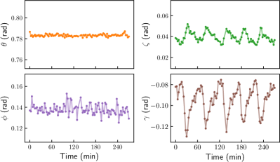
Figure S2: The values of the four (out of five) parameters of our hardware native gate obtained by Floquet calibration. The mechanism of the oscillations in the parameters ζ𝜁\zeta and γ𝛾\gamma is still not completely clear, but likely due to fluctuations in temperature. Since the changes of these two parameters are significant, they must be corrected in real time to obtain desired results.

The n𝑛n-th power of the number-conserving gate reads

Un=diag\scalerel[5pt](\ensurestackMath\addstackgap[1.5pt](1,einγu(θ,ζ,χ)n,ein(2γ+ϕ)\scalerel[5pt])\ensurestackMath\addstackgap[1.5pt]),superscript𝑈𝑛diag1superscript𝑒𝑖𝑛𝛾𝑢superscript𝜃𝜁𝜒𝑛superscript𝑒𝑖𝑛2𝛾italic-ϕ\displaystyle U^{n}=\operatorname{diag}\mathopen{\scalerel*[5pt]{\big{(}}{\ensurestackMath{\addstackgap[1.5pt]{\big{(}}}}}1,\>e^{-in\gamma}u(\theta,\zeta,\chi)^{n},\>e^{-in(2\gamma+\phi)}\mathclose{\scalerel*[5pt]{\big{)}}{\ensurestackMath{\addstackgap[1.5pt]{\big{)}}}}}\,, (28)

where unsuperscript𝑢𝑛u^{n} can be solved using the representation (24),

unsuperscript𝑢𝑛\displaystyle u^{n} =Icos(nΩ)iσ(θ,ζ,χ)sin(nΩ),absent𝐼𝑛Ω𝑖𝜎𝜃𝜁𝜒𝑛Ω\displaystyle=I\cos(n\hskip 0.4pt\Omega)-i\,\sigma(\theta,\zeta,\chi)\sin(n\hskip 0.4pt\Omega)\,, (29)

which takes the matrix form

(cos(nΩ)iΛncosθsinζiΛneiχsinθiΛneiχsinθcos(nΩ)+iΛncosθsinζ),matrix𝑛Ω𝑖subscriptΛ𝑛𝜃𝜁𝑖subscriptΛ𝑛superscript𝑒𝑖𝜒𝜃𝑖subscriptΛ𝑛superscript𝑒𝑖𝜒𝜃𝑛Ω𝑖subscriptΛ𝑛𝜃𝜁\displaystyle\scalebox{0.92}{ $\begin{pmatrix}\cos(n\hskip 0.4pt\Omega)-i\Lambda_{n}\cos\theta\sin\zeta&-i\hskip 0.4pt\Lambda_{n}\hskip 0.4pte^{i\chi}\sin\theta\\[4.0pt] -i\hskip 0.4pt\Lambda_{n}\hskip 0.4pte^{-i\chi}\sin\theta&\cos(n\hskip 0.4pt\Omega)+i\Lambda_{n}\cos\theta\sin\zeta\end{pmatrix}$}\,, (30)

where Λn=sin(nΩ)/sinΩsubscriptΛ𝑛𝑛ΩΩ\Lambda_{n}=\sin(n\hskip 0.4pt\Omega)/\sin\Omega.

To calibrate the gate parameters, we introduce the cycle unitary made up of U𝑈U and singe-qubit Z𝑍Z rotations

Ucsubscript𝑈𝑐\displaystyle U_{c} U(θ,ζ,χ,γ,ϕ)RZ(z1,z2)absent𝑈𝜃𝜁𝜒𝛾italic-ϕsubscript𝑅𝑍subscript𝑧1subscript𝑧2\displaystyle\equiv U(\theta,\zeta,\chi,\gamma,\phi)\,R_{Z}(z_{1},z_{2}) (31)
=U(θ,ζc,χc,γc,ϕ),absent𝑈𝜃subscript𝜁𝑐subscript𝜒𝑐subscript𝛾𝑐italic-ϕ\displaystyle=U(\theta,\zeta_{c},\chi_{c},\gamma_{c},\phi)\,, (32)

where the parameters of Ucsubscript𝑈𝑐U_{c} are related to the original ones via the linear relations

ζc=ζ+z,χc=χ+z,γc=γz+.formulae-sequencesubscript𝜁𝑐𝜁superscript𝑧formulae-sequencesubscript𝜒𝑐𝜒superscript𝑧subscript𝛾𝑐𝛾superscript𝑧\displaystyle\zeta_{c}=\zeta+z^{\scalebox{0.85}{$\scriptstyle-$}}\,,\quad\chi_{c}=\chi+z^{\scalebox{0.85}{$\scriptstyle-$}}\,,\quad\gamma_{c}=\gamma-z^{\scalebox{0.85}{$\scriptstyle+$}}\,. (33)

The two parameters z±=(z1±z2)/2superscript𝑧plus-or-minusplus-or-minussubscript𝑧1subscript𝑧22z^{\scalebox{0.85}{$\scriptstyle\pm$}}=(z_{1}\pm z_{2})/2 can be controlled by adjusting the single-qubit pulses. The hidden assumption here is: the two-qubit gate U𝑈U does not depend on z1subscript𝑧1z_{1} and z2subscript𝑧2z_{2}, i.e., the control pulses do not interleave (no gate bleeding). The cycle unitary has two trivial eigenstates | 00delimited-|⟩00\lvert\,00\,\rangle and | 11delimited-|⟩11\lvert\,11\,\rangle,

Refer to caption
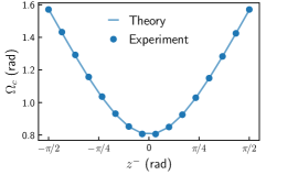
Figure S3: Experiment data for ΩcsubscriptΩ𝑐\Omega_{c} as a function of zsuperscript𝑧z^{\scalebox{0.85}{$\scriptstyle-$}}. They compare well with the fitted curve based on the analytic expression (38). This indicates that gate bleeding between RZsubscript𝑅𝑍R_{Z} and the two-qubit gate U𝑈U is negligible, i.e., their control pulses do not interleave with each other.
Uc| 00=| 00,Uc| 11=ei(2γc+ϕ)| 11\displaystyle U_{c}\lvert\,00\,\rangle=\lvert\,00\,\rangle\,,\quad U_{c}\lvert\,11\,\rangle=e^{-i(2\gamma_{c}+\phi)}\lvert\,11\,\rangle (34)

and two nontrivial eigenstates

|Ψc+delimited-|⟩superscriptsubscriptΨ𝑐\displaystyle\lvert\,\Psi_{c}^{+}\,\rangle =cos(sc/2)| 01+sin(sc/2)eiχc| 10,\displaystyle=\cos(s_{c}/2)\,\lvert\,01\,\rangle+\sin(s_{c}/2)\,e^{-i\chi_{c}}\,\lvert\,10\,\rangle\,, (35)
|Ψcdelimited-|⟩superscriptsubscriptΨ𝑐\displaystyle\lvert\,\Psi_{c}^{-}\,\rangle =sin(sc/2)| 01cos(sc/2)eiχc| 10,\displaystyle=\sin(s_{c}/2)\,\lvert\,01\,\rangle-\cos(s_{c}/2)\,e^{-i\chi_{c}}\,\lvert\,10\,\rangle\,, (36)

where sc=arccot(cotθsinζc)subscript𝑠𝑐arccot𝜃subscript𝜁𝑐s_{c}=\operatorname{arccot}(\cot\theta\sin\zeta_{c}). The corresponding eigenvalue equations are

Uc|Ψc±=ei(γc±Ωc)|Ψc±,\displaystyle U_{c}\lvert\,\Psi^{\pm}_{c}\,\rangle=e^{-i(\gamma_{c}\pm\Omega_{c})}\hskip 0.4pt\lvert\,\Psi^{\pm}_{c}\,\rangle\,, (37)

where Ωc[θ,πθ]subscriptΩ𝑐𝜃𝜋𝜃\Omega_{c}\in[\theta,\pi-\theta] is the Rabi angle

Ωc=arccos(cosθcos(ζ+z)).subscriptΩ𝑐𝜃𝜁superscript𝑧\displaystyle\Omega_{c}=\arccos\bigl{(}\cos\theta\cos(\zeta+z^{\scalebox{0.85}{$\scriptstyle-$}})\bigr{)}\,. (38)

Knowing the eigenvalues of Ucsubscript𝑈𝑐U_{c} allows one to learn γcsubscript𝛾𝑐\gamma_{c}, ΩcsubscriptΩ𝑐\Omega_{c}, and ϕitalic-ϕ\phi, from which one can learn γ𝛾\gamma using the last identity in Eq. (33). To learn θ𝜃\theta and ζ𝜁\zeta using Eq. (38), one needs to know ΩcsubscriptΩ𝑐\Omega_{c} for at least two different values of zsuperscript𝑧z^{\scalebox{0.85}{$\scriptstyle-$}}. In Fig. S3, we plot the experiment results for ΩcsubscriptΩ𝑐\Omega_{c} as a function of zsuperscript𝑧z^{\scalebox{0.85}{$\scriptstyle-$}} and compare them with the fitted curve based on Eq. (38). They conform extremely well with each other, indicating that gate bleeding between the single-qubit Z𝑍Z rotations and the two-qubit U𝑈U is negligible.

In the following, we introduce three sets of calibration circuits to learn the five parameters in the number-conserving gate (C1). We run each set of circuits with the cycle repetition numbers from the set

={rk|k=0,1,,K1},r>0.\displaystyle\mathbb{N}=\bigl{\{}\lceil r^{k}\rceil\,\big{\lvert}\,k=0,1,\ldots,K-1\bigr{\}}\,,\quad r>0\,. (39)

This is necessary because the eigenvalues of Ucsubscript𝑈𝑐U_{c} can only be determined up to modulo 2π/n2𝜋𝑛2\pi/n when Ucsubscript𝑈𝑐U_{c} is repeated for n𝑛n times. To make sure that we search in the correct principal region, the true value should be located within the (π/n)𝜋𝑛(\pi/n)-neighborhood of the prior estimate with high probability. We will discuss this issue and how to choose the real number r𝑟r in more detail in Section C2.

Calibration circuits 1

This set of calibration circuits are used to learn the parameters θ𝜃\theta and ζ𝜁\zeta in the gate (C1), see Fig. S4. The probability of measuring the state | 10delimited-|⟩10\lvert\,10\,\rangle is

pnsubscript𝑝𝑛\displaystyle p_{n} =| 10|UcnRX(0,π)| 00|2\displaystyle=\big{\lvert}\langle\,10\,\rvert\,U_{c}^{n}R_{X}(0,\pi)\lvert\,00\,\rangle\big{\rvert}^{2}
=| 1|ucn| 0|2=\scalerel[5pt](\ensurestackMath\addstackgap[1.5pt](sin(nΩc)sinθ/sinΩc\scalerel[5pt])\ensurestackMath\addstackgap[1.5pt])2,\displaystyle=\big{\lvert}\langle\,1\,\rvert u_{c}^{n}\lvert\,0\,\rangle\big{\rvert}^{2}=\mathopen{\scalerel*[5pt]{\big{(}}{\ensurestackMath{\addstackgap[1.5pt]{\big{(}}}}}\sin(n\hskip 0.4pt\Omega_{c})\sin\theta/\sin\Omega_{c}\mathclose{\scalerel*[5pt]{\big{)}}{\ensurestackMath{\addstackgap[1.5pt]{\big{)}}}}}^{2}\,, (40)

where ucnu(θ,ζc,χc)nsuperscriptsubscript𝑢𝑐𝑛𝑢superscript𝜃subscript𝜁𝑐subscript𝜒𝑐𝑛u_{c}^{n}\equiv u(\theta,\zeta_{c},\chi_{c})^{n} is given in Eq. (30).

Refer to caption
Figure S4: The circuit to calibrate the parameters θ𝜃\theta and ζ𝜁\zeta in the excitation-number-conserving gate. The cycle unitary is repeated for n𝑛n times before we measure the qubits in the Z𝑍Z basis.

By postselecting the measurement results with one excitation, i.e., | 01delimited-|⟩01\lvert\,01\,\rangle and | 10delimited-|⟩10\lvert\,10\,\rangle, we make the results robust to T1subscript𝑇1T_{1} error and bit-flip errors in the measurement. An unbiased estimator of pnsubscript𝑝𝑛p_{n} based on the measurement results is

p^n=Number of outcome 10Number of outcomes 01 and 10,subscript^𝑝𝑛Number of outcome 10Number of outcomes 01 and 10\displaystyle\hat{p}_{n}=\frac{\text{Number of outcome 10}}{\text{Number of outcomes 01 and 10}}\,, (41)

and its variance decreases as the number of measurements passing postselection (the denominator) increases.

Using Eqs. (38) and (C1), we can relate the measurement probability pnsubscript𝑝𝑛p_{n} to the gate parameters θ𝜃\theta and ζ𝜁\zeta and the adjustable variable zsuperscript𝑧z^{\scalebox{0.85}{$\scriptstyle-$}}. For n=1,2𝑛12n=1,2, we have

|sinθ|=p1,sin(2θ)|cos(ζ+z)|=p2,formulae-sequence𝜃subscript𝑝12𝜃𝜁superscript𝑧subscript𝑝2\displaystyle\lvert\sin\theta\rvert=\sqrt{p_{1}}\,,\quad\sin(2\theta)\,\lvert\cos(\zeta+z^{\scalebox{0.85}{$\scriptstyle-$}})\rvert=\sqrt{p_{2}}\,, (42)

which can be used to get initial estimates of θ𝜃\theta and ζ𝜁\zeta. To get robust estimates for larger n𝑛n, we use aggregated results from several previous runs by introducing the cost function (we use the Hellinger distance, but other metrics might work as well)

Cn(x,y)superscriptsubscript𝐶𝑛𝑥𝑦\displaystyle C_{n}^{\ell}(x,y)
=mnmzm(|sin(mΩc)sinxsinΩc|p^m,z)2,absentsubscript𝑚𝑛𝑚subscriptsuperscript𝑧superscriptsubscript𝑚superscript𝑚subscriptΩ𝑐𝑥subscriptΩ𝑐subscript^𝑝𝑚superscript𝑧2\displaystyle\hskip 3.99994pt=\!\sum_{\begin{subarray}{c}\ell\leq m\leq n\\[1.0pt] m\in\mathbb{N}\end{subarray}}\!\sum_{\;\;z^{\scalebox{0.85}{$\scriptstyle-$}}\in\mathbb{Z}_{m}^{-}}\biggl{(}\Bigl{\lvert}\frac{\sin(m\hskip 0.4pt\Omega_{c})\sin x}{\sin\Omega_{c}}\Bigr{\rvert}-\sqrt{\hat{p}_{m,\hskip 0.4ptz^{\scalebox{0.85}{$\scriptstyle-$}}}}\biggr{)}^{2}\,, (43)

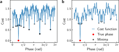
where Ωc(x,y,z)=arccos(cosxcos(y+z))subscriptΩ𝑐𝑥𝑦superscript𝑧𝑥𝑦superscript𝑧\Omega_{c}(x,y,z^{\scalebox{0.85}{$\scriptstyle-$}})=\arccos\bigl{(}\cos x\cos(y+z^{\scalebox{0.85}{$\scriptstyle-$}})\bigr{)} and the lower bound \ell determines the number of terms included in the cost function. This approach also provides us with the flexibility of using a different set of zsuperscript𝑧z^{\scalebox{0.85}{$\scriptstyle-$}} for each cycle repetition number m𝑚m, which we denote as msuperscriptsubscript𝑚\mathbb{Z}_{m}^{-}. When n𝑛n is small, we use the global minimum of the cost function as the estimators of θ𝜃\theta and ζ𝜁\zeta. For larger n𝑛n, the landscape of the cost function becomes rugged, and we use its local minimum around the prior estimates as the new estimates. We choose \ell based on the following rules. For small n𝑛n, it is easy to get into the wrong principal regions, and we include all the prior runs in the cost function by setting =11\ell=1. As n𝑛n increases, we fix the number of terms in the cost function by increasing \ell. We then gradually reduce the number of terms in the cost function to minimize the variance of the estimates at the end.

The variances of the estimates of θ𝜃\theta and ζ𝜁\zeta diverge when either |Ωc/θ|subscriptΩ𝑐𝜃\lvert\partial\Omega_{c}/\partial\theta\rvert or |Ωc/ζ|subscriptΩ𝑐𝜁\lvert\partial\Omega_{c}/\partial\zeta\rvert is close to zero. This can be avoided by adaptively choosing the values of zsuperscript𝑧z^{\scalebox{0.85}{$\scriptstyle-$}} based on the current estimates of θ𝜃\theta and ζ𝜁\zeta. We may choose the two values of zsuperscript𝑧z^{\scalebox{0.85}{$\scriptstyle-$}} close to π/4𝜋4\pi/4 and 3π/43𝜋43\pi/4, which are apart by π/2𝜋2\pi/2 for best performance. This choice also leaves a large margin between ζc(modπ/2)subscript𝜁𝑐modulo𝜋2\zeta_{c}\;(\mathord{\bmod}\;\pi/2) and 00 for small ζ𝜁\zeta, where either |Ωc/θ|subscriptΩ𝑐𝜃\lvert\partial\Omega_{c}/\partial\theta\rvert or |Ωc/ζ|subscriptΩ𝑐𝜁\lvert\partial\Omega_{c}/\partial\zeta\rvert equals to zero. The standard error in the estimate of ΩcsubscriptΩ𝑐\Omega_{c} is inversely proportional to the derivative

pnΩcnsin(2nΩc)(sinθ/sinΩc)2,similar-to-or-equalssubscript𝑝𝑛subscriptΩ𝑐𝑛2𝑛subscriptΩ𝑐superscript𝜃subscriptΩ𝑐2\displaystyle\frac{\partial p_{n}}{\partial\Omega_{c}}\simeq n\sin(2n\hskip 0.4pt\Omega_{c})\,\bigl{(}\sin\theta/\sin\Omega_{c}\bigr{)}^{2}\,, (44)

where we assume n1much-greater-than𝑛1n\gg 1 and neglect terms of order 𝒪(1)𝒪1\mathcal{O}(1). We maximize the fast oscillating part sin(2nΩc)2𝑛subscriptΩ𝑐\sin(2n\hskip 0.4pt\Omega_{c}) in Eq.(44) by choosing zsuperscript𝑧z^{\scalebox{0.85}{$\scriptstyle-$}} from the neighborhood of π/4𝜋4\pi/4 and 3π/43𝜋43\pi/4 such that

nΩc=π/4(modπ/2),𝑛subscriptΩ𝑐𝜋4modulo𝜋2\displaystyle n\,\Omega_{c}=\pi/4\;(\mathord{\bmod}\;\pi/2)\,, (45)

where ΩcsubscriptΩ𝑐\Omega_{c} is evaluated using the estimates of θ𝜃\theta and ζ𝜁\zeta.

These calibration circuits can also be implemented non-adaptively at the price of increasing the number of circuits. We run the circuit in Fig. S4 for several equidistant values of zsuperscript𝑧z^{\scalebox{0.85}{$\scriptstyle-$}} in the two intervals π/4±w/nplus-or-minus𝜋4𝑤𝑛\pi/4\pm w/n and 3π/4±w/nplus-or-minus3𝜋4𝑤𝑛3\pi/4\pm w/n, where w=π/(2cosθ)𝑤𝜋2𝜃w=\pi/(2\cos\theta). This choice guarantees that Eq. (44) has big values at least for some of the selected values of zsuperscript𝑧z^{\scalebox{0.85}{$\scriptstyle-$}}. The values of θ𝜃\theta and ζ𝜁\zeta can then be estimated by fitting the data to Eq. (C1).

Calibration circuits 2

Refer to caption
Figure S5: The circuit to calibrate the parameters γ𝛾\gamma and χ𝜒\chi in the general FSIMFSIM\mathrm{FSIM} gate. The initial X𝑋\sqrt{X} gate creates a superposition between the state | 00delimited-|⟩00\lvert\,00\,\rangle and the single-excitation state | 01delimited-|⟩01\lvert\,01\,\rangle.

Here we will focus on γ𝛾\gamma and χ𝜒\chi, since θ𝜃\theta and ζ𝜁\zeta can be better estimated with the former calibration circuits. The circuit in Fig. S5 can be used to measure the accumulated phase nγ+χ𝑛𝛾𝜒n\gamma+\chi, from which one can estimate γ𝛾\gamma with high precision. In comparison, χ𝜒\chi can only be estimated with low precision (also susceptible to SPAM errors) due to lack of the scaling factor n𝑛n. Consider the measurement probabilities for the circuit in Fig. S5,

pnsubscript𝑝𝑛\displaystyle p_{n} =| 00|RX(π/2,0)UcnRX(0,π/2)| 00|2\displaystyle=\big{\lvert}\langle\,00\,\rvert R_{X}(\pi/2,0)\,U_{c}^{n}R_{X}(0,\pi/2)\,\lvert\,00\,\rangle\big{\rvert}^{2}
=14|einγc 1|ucn| 0|2,\displaystyle=\frac{1}{4}\,\big{\lvert}e^{in\gamma_{c}}-\langle\,1\,\rvert\,u_{c}^{n}\lvert\,0\,\rangle\big{\rvert}^{2}\,, (46)

and

qnsubscript𝑞𝑛\displaystyle q_{n} =| 01|RX(π/2,0)UcnRX(0,π/2)| 00|2\displaystyle=\big{\lvert}\langle\,01\,\rvert R_{X}(\pi/2,0)\,U_{c}^{n}R_{X}(0,\pi/2)\,\lvert\,00\,\rangle\big{\rvert}^{2}
=14| 0|ucn| 0|2.\displaystyle=\frac{1}{4}\,\lvert\langle\,0\,\rvert\,u_{c}^{n}\lvert\,0\,\rangle\rvert^{2}\,. (47)

To estimate the parameter γc=γz+subscript𝛾𝑐𝛾superscript𝑧\gamma_{c}=\gamma-z^{\scalebox{0.85}{$\scriptstyle+$}} using Eq. (C1), we will need to learn  1|ucn| 0\langle\,1\,\rvert u_{c}^{n}\lvert\,0\,\rangle. Its phase can be calculated using Eq. (30),

arg( 1|ucn| 0)\displaystyle\arg(\langle\,1\,\rvert\,u_{c}^{n}\lvert\,0\,\rangle) =χzπ2sgnΛn,absent𝜒superscript𝑧𝜋2sgnsubscriptΛ𝑛\displaystyle=-\chi-z^{\scalebox{0.85}{$\scriptstyle-$}}-\frac{\pi}{2}\operatorname{sgn}\Lambda_{n}\,, (48)

where Λn=sin(nΩc)/sinΩcsubscriptΛ𝑛𝑛subscriptΩ𝑐subscriptΩ𝑐\Lambda_{n}=\sin(n\hskip 0.4pt\Omega_{c})/\sin\Omega_{c} and its sign can be determined with confidence provided that we have good estimates of θ𝜃\theta and ζ𝜁\zeta. Using the normalization condition | 0|ucn| 0|2+| 1|ucn| 0|2=1\lvert\langle\,0\,\rvert\,u_{c}^{n}\lvert\,0\,\rangle\rvert^{2}+\lvert\langle\,1\,\rvert\,u_{c}^{n}\lvert\,0\,\rangle\rvert^{2}=1, we have

| 1|ucn| 0|=14qn.\displaystyle\lvert\langle\,1\,\rvert\,u_{c}^{n}\lvert\,0\,\rangle\rvert=\sqrt{1-4q_{n}}\,. (49)

The measurement probability pnsubscript𝑝𝑛p_{n} in Eq. (C1) is a function of | 1|ucn| 0|\lvert\langle\,1\,\rvert\,u_{c}^{n}\lvert\,0\,\rangle\rvert and the relative phase

μnsubscript𝜇𝑛\displaystyle\mu_{n} =nγcarg( 1|ucn| 0)\displaystyle=n\gamma_{c}-\arg(\langle\,1\,\rvert\,u_{c}^{n}\lvert\,0\,\rangle) (50)
=(nγ+χ)nz++z+π2sgnΛn.absent𝑛𝛾𝜒𝑛superscript𝑧superscript𝑧𝜋2sgnsubscriptΛ𝑛\displaystyle=(n\gamma+\chi)-nz^{\scalebox{0.85}{$\scriptstyle+$}}+z^{\scalebox{0.85}{$\scriptstyle-$}}+\frac{\pi}{2}\operatorname{sgn}\Lambda_{n}\,. (51)

Knowing μnsubscript𝜇𝑛\mu_{n} for different values of n𝑛n allows one to estimate γ𝛾\gamma and χ𝜒\chi. It is related to the measurement probabilities through the relation

|eiμn14qn|2=4pn,superscriptsuperscript𝑒𝑖subscript𝜇𝑛14subscript𝑞𝑛24subscript𝑝𝑛\displaystyle\big{\lvert}e^{i\mu_{n}}-\sqrt{1-4q_{n}}\>\big{\rvert}^{2}=4p_{n}\,, (52)

or equivalently

cosμn=12(pn+qn)14qn.subscript𝜇𝑛12subscript𝑝𝑛subscript𝑞𝑛14subscript𝑞𝑛\displaystyle\cos\mu_{n}=\frac{1-2(p_{n}+q_{n})}{\sqrt{1-4q_{n}}}\,. (53)

Again, we introduce the cost function

Cn(x,y)superscriptsubscript𝐶𝑛𝑥𝑦\displaystyle C_{n}^{\ell}(x,y) =mnm(fn(x,y)12(p^n+q^n)14q^n)2,absentsubscript𝑚𝑛𝑚superscriptsubscript𝑓𝑛𝑥𝑦12subscript^𝑝𝑛subscript^𝑞𝑛14subscript^𝑞𝑛2\displaystyle=\sum_{\begin{subarray}{c}\ell\leq m\leq n\\[1.0pt] m\in\mathbb{N}\end{subarray}}\biggl{(}f_{n}(x,y)-\frac{1-2(\hat{p}_{n}+\hat{q}_{n})}{\sqrt{1-4\hat{q}_{n}}}\,\biggr{)}^{2}\,, (54)

where fn(x,y)=cos(nx+ynz++z+π2sgnΛn)subscript𝑓𝑛𝑥𝑦𝑛𝑥𝑦𝑛superscript𝑧superscript𝑧𝜋2sgnsubscriptΛ𝑛f_{n}(x,y)=\cos(nx+y-nz^{\scalebox{0.85}{$\scriptstyle+$}}+z^{\scalebox{0.85}{$\scriptstyle-$}}+\frac{\pi}{2}\operatorname{sgn}\Lambda_{n}). The parameters γ𝛾\gamma and χ𝜒\chi can be estimated by using the arguments x𝑥x and y𝑦y that minimize the cost function, respectively. We follow the same prescription as in the former case to choose \ell and minimize the cost function.

To reduce the variances of estimators, we choose zsuperscript𝑧z^{\scalebox{0.85}{$\scriptstyle-$}} such that | 1|ucn| 0|\lvert\langle\,1\,\rvert u_{c}^{n}\lvert\,0\,\rangle\rvert is maximized using the estimates of θ𝜃\theta and ζ𝜁\zeta. We also choose z+superscript𝑧z^{\scalebox{0.85}{$\scriptstyle+$}} such that μnπ/2(modπ)similar-to-or-equalssubscript𝜇𝑛𝜋2modulo𝜋\mu_{n}\simeq\pi/2\;(\mathord{\bmod}\;\pi), which maximizes |pn/μn|subscript𝑝𝑛subscript𝜇𝑛\lvert\partial p_{n}/\partial\mu_{n}\rvert. It also leaves a big margin (close to π𝜋\pi) between μnsubscript𝜇𝑛\mu_{n} and other phases sharing the same cosine value; this reduces the chance of misidentification of the phase. We can also implement this non-adaptively by running two values of z+superscript𝑧z^{\scalebox{0.85}{$\scriptstyle+$}} apart by π/2𝜋2\pi/2, which allows for estimating any phase to the same precision.

Calibration circuits 3

This set of circuits can be used to estimate θ𝜃\theta, ζ𝜁\zeta, and γ+ϕ𝛾italic-ϕ\gamma+\phi with high precision, see Fig. S6.

Refer to caption
Figure S6: The circuit to calibrate the parameter ϕitalic-ϕ\phi. The initial microwave gates create a superposition between the state | 11delimited-|⟩11\lvert\,11\,\rangle and the single-excitation state | 01delimited-|⟩01\lvert\,01\,\rangle.

We will focus on γ+ϕ𝛾italic-ϕ\gamma+\phi, from which we can derive the value of the controlled phase ϕitalic-ϕ\phi given that γ𝛾\gamma is known. Consider the measurement probabilities

pnsubscript𝑝𝑛\displaystyle p_{n} =| 10|RX(0,π/2)UcnRX(π/2,π)| 00|2\displaystyle=\big{\lvert}\langle\,10\,\rvert R_{X}(0,\pi/2)\,U_{c}^{n}R_{X}(\pi/2,\pi)\,\lvert\,00\,\rangle\big{\rvert}^{2} (55)
=14|ein(γc+ϕ) 1|ucn| 0|2,\displaystyle=\frac{1}{4}\,\big{\lvert}e^{-in(\gamma_{c}+\phi)}-\langle\,1\,\rvert\,u_{c}^{n}\lvert\,0\,\rangle\big{\rvert}^{2}\,, (56)
qnsubscript𝑞𝑛\displaystyle q_{n} =| 00|RX(0,π/2)UcnRX(π/2,π)| 00|2\displaystyle=\big{\lvert}\langle\,00\,\rvert R_{X}(0,\pi/2)\,U_{c}^{n}R_{X}(\pi/2,\pi)\,\lvert\,00\,\rangle\big{\rvert}^{2} (57)
=14| 0|ucn| 0|2.\displaystyle=\frac{1}{4}\,\lvert\langle\,0\,\rvert\,u_{c}^{n}\lvert\,0\,\rangle\rvert^{2}\,. (58)

We define the relative phase

μnsubscript𝜇𝑛\displaystyle\mu_{n} =n(γc+ϕ)arg( 1|ucn| 0)\displaystyle=-n(\gamma_{c}+\phi)-\arg(\langle\,1\,\rvert\,u_{c}^{n}\lvert\,0\,\rangle) (59)
=n(γ+ϕ)+χ+nz++z+π2sgnΛ,absent𝑛𝛾italic-ϕ𝜒𝑛superscript𝑧superscript𝑧𝜋2sgnΛ\displaystyle=-n(\gamma+\phi)+\chi+nz^{\scalebox{0.85}{$\scriptstyle+$}}+z^{\scalebox{0.85}{$\scriptstyle-$}}+\frac{\pi}{2}\operatorname{sgn}\Lambda\,, (60)

which can be estimated using the same procedure as the last case.

C2 Phase estimation under decoherence

Quantum metrology protocols are typically extremely sensitive to noise [shaji_qubit_2007]. For example, the depolarizing noise—no matter how small—ruins the possibility of sub-shot-noise performances of a quantum interferometer [ji_parameter_2008]. It was also demonstrated that quantum metrology can only do better than classical approaches by a constant factor for any nonzero loss [kolodynski_phase_2010, knysh_scaling_2011]. In this section, we discuss the decoherence effects on single- and two-qubit phase estimation.

Consider a single-qubit system described by the master equation ρ˙=i[H,ρ]+(ρ)˙𝜌𝑖Planck-constant-over-2-pi𝐻𝜌𝜌\dot{\rho}=-\frac{i}{\hbar}[H,\,\rho]+\mathcal{L}(\rho), where the Lindblad operator (ρ)𝜌\mathcal{L}(\rho) takes the form

(ρ)𝜌\displaystyle\mathcal{L}(\rho) =1T1(σρσ+12(σ+σρ+ρσ+σ))absent1subscript𝑇1superscript𝜎𝜌superscript𝜎12superscript𝜎superscript𝜎𝜌𝜌superscript𝜎superscript𝜎\displaystyle=\frac{1}{T_{1}}\Big{(}\sigma^{-}\rho\hskip 0.4pt\sigma^{+}-\frac{1}{2}(\sigma^{+}\sigma^{-}\rho+\rho\sigma^{+}\sigma^{-})\Big{)}
+12T2(σzρσzρ).12subscript𝑇2superscript𝜎𝑧𝜌superscript𝜎𝑧𝜌\displaystyle\quad+\frac{1}{2\hskip 0.4ptT_{2}}\left(\sigma^{z}\rho\hskip 0.4pt\sigma^{z}-\rho\right)\,. (61)

We prepare the initial state |ψin=(| 0+| 1)/2\lvert\,\psi_{\mathrm{in}}\,\rangle=(\lvert\,0\,\rangle+\lvert\,1\,\rangle)/\sqrt{2} and apply the phase gate RZ(φ)=diag(1,eiφ)subscript𝑅𝑍𝜑diag1superscript𝑒𝑖𝜑R_{Z}(\varphi)=\operatorname{diag}(1,e^{i\varphi}) for n𝑛n times. We then apply another phase shift diag(1,eis)diag1superscript𝑒𝑖𝑠\operatorname{diag}(1,e^{is}) before measuring the system in the X𝑋X basis. The probability that an excitation does not decay after n𝑛n gate cycles is enλ1superscript𝑒𝑛subscript𝜆1e^{-n\lambda_{1}}, where λ1=gate time/T1subscript𝜆1gate timesubscript𝑇1\lambda_{1}=\text{gate time}/T_{1}. Therefore, the probability of getting the measurement outcome ++ is

pn(s)=enλ1qn(s)+1enλ12,subscript𝑝𝑛𝑠superscript𝑒𝑛subscript𝜆1subscript𝑞𝑛𝑠1superscript𝑒𝑛subscript𝜆12\displaystyle p_{n}(s)=e^{-n\lambda_{1}}q_{n}(s)+\frac{1-e^{-n\lambda_{1}}}{2}\,, (62)

where qn(s)subscript𝑞𝑛𝑠q_{n}(s) is the probability of getting the outcome ++ with only T2subscript𝑇2T_{2} error

qn(s)=1+enλ2cos(nφ+s)2,subscript𝑞𝑛𝑠1superscript𝑒𝑛subscript𝜆2𝑛𝜑𝑠2\displaystyle q_{n}(s)=\frac{1+e^{-n\lambda_{2}}\cos(n\hskip 0.4pt\varphi+s)}{2}\,, (63)

where λ2=gate time/T2subscript𝜆2gate timesubscript𝑇2\lambda_{2}=\text{gate time}/T_{2}. An unbiased estimator of the probability pnsubscript𝑝𝑛p_{n} is

p^n=Number of outcome +Mn,subscript^𝑝𝑛Number of outcome +subscript𝑀𝑛\displaystyle\hat{p}_{n}=\frac{\text{Number of outcome +}}{M_{n}}\,, (64)

where Mnsubscript𝑀𝑛M_{n} is the circuit repetition number. The variance of the estimator p^nsubscript^𝑝𝑛\hat{p}_{n} is

V(p^n)𝑉subscript^𝑝𝑛\displaystyle V(\hat{p}_{n}) =pn(1pn)Mnabsentsubscript𝑝𝑛1subscript𝑝𝑛subscript𝑀𝑛\displaystyle=\frac{p_{n}(1-p_{n})}{M_{n}} (65)
=e2nλ1qn(1qn)Mn+1e2nλ14Mn,absentsuperscript𝑒2𝑛subscript𝜆1subscript𝑞𝑛1subscript𝑞𝑛subscript𝑀𝑛1superscript𝑒2𝑛subscript𝜆14subscript𝑀𝑛\displaystyle=\frac{e^{-2n\lambda_{1}}q_{n}(1-q_{n})}{M_{n}}+\frac{1-e^{-2n\lambda_{1}}}{4M_{n}}\,, (66)

and the variance of the estimator of φ𝜑\varphi can be determined using the chain rule

V(φ^n)𝑉subscript^𝜑𝑛\displaystyle V(\hat{\varphi}_{n}) =V(p^n)(pn/qn)2(qn/φ)2absent𝑉subscript^𝑝𝑛superscriptsubscript𝑝𝑛subscript𝑞𝑛2superscriptsubscript𝑞𝑛𝜑2\displaystyle=\frac{V(\hat{p}_{n})}{(\partial p_{n}/\partial q_{n})^{2}\,(\partial q_{n}/\partial\varphi)^{2}} (67)
=e2nλ1e2nλ2cos(nφ+s)2Mnn2e2nλ2sin(nφ+s)2\displaystyle=\frac{e^{2n\lambda_{1}}-e^{-2n\lambda_{2}}\cos(n\hskip 0.4pt\varphi+s)^{2}}{M_{n}\hskip 0.4ptn^{2}\hskip 0.4pte^{-2n\lambda_{2}}\hskip 0.4pt\sin(n\hskip 0.4pt\varphi+s)^{2}} (68)
e2n(λ1+λ2)Mnn2sin(nφ+s)2.\displaystyle\leq\frac{e^{2n(\lambda_{1}+\lambda_{2})}}{M_{n}\hskip 0.4ptn^{2}\hskip 0.4pt\sin(n\hskip 0.4pt\varphi+s)^{2}}\,. (69)

Equation (69) diverges when sin(nφ+s)=0𝑛𝜑𝑠0\sin(n\hskip 0.4pt\varphi+s)=0, which can be avoided by adjusting the phase shift s𝑠s adaptively. One can also implement this non-adaptively by running two experiments at s=0𝑠0s=0 and s=π/2𝑠𝜋2s=\pi/2. Using the combined information of the two, we have

V(φ^n)e2n(λ1+λ2)Mnn2.𝑉subscript^𝜑𝑛superscript𝑒2𝑛subscript𝜆1subscript𝜆2subscript𝑀𝑛superscript𝑛2\displaystyle V(\hat{\varphi}_{n})\leq\frac{e^{2n(\lambda_{1}+\lambda_{2})}}{M_{n}\hskip 0.4ptn^{2}}\,. (70)

Therefore, the standard deviation of the estimator φ^nsubscript^𝜑𝑛\hat{\varphi}_{n} decreases as n1superscript𝑛1n^{-1} before it blows exponentially. By setting V(φ^n)/n=0𝑉subscript^𝜑𝑛𝑛0\partial V(\hat{\varphi}_{n})/\partial n=0, we have

n=1λ1+λ21,V(φ^n)e2(λ1+λ2)2Mn.formulae-sequencesubscript𝑛1subscript𝜆1subscript𝜆2much-greater-than1𝑉subscript^𝜑subscript𝑛superscript𝑒2superscriptsubscript𝜆1subscript𝜆22subscript𝑀subscript𝑛\displaystyle n_{\star}=\frac{1}{\lambda_{1}+\lambda_{2}}\gg 1\,,\quad V(\hat{\varphi}_{n_{\star}})\leq\frac{e^{2}(\lambda_{1}+\lambda_{2})^{2}}{M_{n_{\star}}}\,. (71)

The minimum variance that one can achieve is therefore set by λ1+λ2subscript𝜆1subscript𝜆2\lambda_{1}+\lambda_{2}. If the estimator φ^nsubscript^𝜑𝑛\hat{\varphi}_{n} is unbiased, the minimum variance that one can achieve is bounded by

V(φ^)(n1V(φ^n))1=1F,𝑉^𝜑superscriptsubscript𝑛1𝑉subscript^𝜑𝑛11𝐹\displaystyle V(\hat{\varphi})\geq\bigg{(}\sum_{n\in\mathbb{N}}\frac{1}{V(\hat{\varphi}_{n})}\bigg{)}^{-1}=\frac{1}{F}\,, (72)

where F𝐹F is the Fisher information and \mathbb{N} is the set of the cycle repetition numbers. The equal sign in Eq. (72) is achieved by using

φ^=1Fnφ^nV(φ^n).^𝜑1𝐹subscript𝑛subscript^𝜑𝑛𝑉subscript^𝜑𝑛\displaystyle\hat{\varphi}=\frac{1}{F}\,\sum_{n\in\mathbb{N}}\frac{\hat{\varphi}_{n}}{V(\hat{\varphi}_{n})}\,. (73)

For the two-qubit case, the impact of decoherence usually depends on the specific shapes of the control pulses. For simplicity, we consider the resonant case Ωc=θsubscriptΩ𝑐𝜃\Omega_{c}=\theta (or equivalently ζc=0subscript𝜁𝑐0\zeta_{c}=0) of the two-qubit number conserving gate, where the decoherence effects are pulse-shape independent. After removing the T1subscript𝑇1T_{1} error using postselection, the measurement probability in Eq. (C1) reads

pn=1e2nλ2cos(2nθ)2,subscript𝑝𝑛1superscript𝑒2𝑛subscript𝜆22𝑛𝜃2\displaystyle p_{n}=\frac{1-e^{-2n\lambda_{2}}\cos(2n\hskip 0.4pt\theta)}{2}\,, (74)

where the exponential factor comes from dephasing of the two qubits. The variance of the estimator p^nsubscript^𝑝𝑛\hat{p}_{n} is

V(p^n)=pn(1pn)Mnenλ1,𝑉subscript^𝑝𝑛subscript𝑝𝑛1subscript𝑝𝑛subscript𝑀𝑛superscript𝑒𝑛subscript𝜆1\displaystyle V(\hat{p}_{n})=\frac{p_{n}(1-p_{n})}{M_{n}\hskip 0.4pte^{-n\lambda_{1}}}\,, (75)

where Mnenλ1subscript𝑀𝑛superscript𝑒𝑛subscript𝜆1M_{n}\hskip 0.4pte^{-n\lambda_{1}} is the number of measurement pass the post selection. The variance of the estimator of θ𝜃\theta can be calculated by the chain rule

V(θ^n)𝑉subscript^𝜃𝑛\displaystyle V(\hat{\theta}_{n}) =V(p^n)(pn/θ)2absent𝑉subscript^𝑝𝑛superscriptsubscript𝑝𝑛𝜃2\displaystyle=\frac{V(\hat{p}_{n})}{(\partial p_{n}/\partial\theta)^{2}} (76)
=1e4nλ2cos(2nθ)24Mnn2en(λ1+4λ2)sin(2nθ)2\displaystyle=\frac{1-e^{-4n\lambda_{2}}\cos(2n\hskip 0.4pt\theta)^{2}}{4M_{n}\hskip 0.4ptn^{2}\hskip 0.4pte^{-n(\lambda_{1}+4\lambda_{2})}\hskip 0.4pt\sin(2n\hskip 0.4pt\theta)^{2}} (77)
en(λ1+4λ2)4Mnn2sin(2nθ)2.\displaystyle\leq\frac{e^{n(\lambda_{1}+4\lambda_{2})}}{4M_{n}\hskip 0.4ptn^{2}\hskip 0.4pt\sin(2n\hskip 0.4pt\theta)^{2}}\,. (78)

Compared to the single-qubit case (69), the effect of λ1subscript𝜆1\lambda_{1} is reduced by a factor of two due to post selection while the effect of λ2subscript𝜆2\lambda_{2} is doubled due to the dephasing from two qubits. By setting V(θ^n)/n=0𝑉subscript^𝜃𝑛𝑛0\partial V(\hat{\theta}_{n})/\partial n=0, we have

n=2λ1+4λ21,V(θ^n)e2(λ1+4λ2)24m.formulae-sequencesubscript𝑛2subscript𝜆14subscript𝜆2much-greater-than1𝑉subscript^𝜃subscript𝑛superscript𝑒2superscriptsubscript𝜆14subscript𝜆224𝑚\displaystyle n_{\star}=\frac{2}{\lambda_{1}+4\lambda_{2}}\gg 1\,,\quad V(\hat{\theta}_{n_{\star}})\leq\frac{e^{2}\hskip 0.4pt(\lambda_{1}+4\lambda_{2})^{2}}{4m}\,. (79)

C3 Cycle repetition numbers

When the SPAM errors are large, the estimates from prior runs with smaller cycle repetition numbers can fail to locate the principal region of the true value. As a result, one gets estimates with higher and higher resolutions, but in a completely wrong region. Here we briefly discuss how to overcome this issue by properly choosing the set of cycle repetition numbers \mathbb{N}. Consider the cost function to estimate a single-qubit phase φ𝜑\varphi,

Cn(x)subscript𝐶𝑛𝑥\displaystyle C_{n}(x) =m,mn|eimxeimφ^|2,absentsubscript𝑚𝑚𝑛superscriptsuperscript𝑒𝑖𝑚𝑥^superscript𝑒𝑖𝑚𝜑2\displaystyle=\sum_{\begin{subarray}{c}m\in\mathbb{N}\end{subarray},\,m\leq n}\big{\lvert}e^{im\hskip 0.4ptx}-\widehat{e^{im\varphi}}\big{\rvert}^{2}\;, (80)

where eimφ^^superscript𝑒𝑖𝑚𝜑\widehat{e^{im\varphi}} is the estimate of eimφsuperscript𝑒𝑖𝑚𝜑e^{im\varphi} using quantum circuits with cycle repetition number m𝑚m.

Refer to caption
Figure S7: Comparison of two ideal cost functions using exponential circuit repetition numbers rksuperscript𝑟𝑘r^{k}. Left: exponent r=2𝑟2r=2 with 777 runs, i.e., n=1,2,4,8,16,32,64𝑛1248163264n=1,2,4,8,16,32,64. Right: exponent r=1.9𝑟1.9r=1.9 with 777 runs, i.e., n=1,2,4,7,14,25,48𝑛1247142548n=1,2,4,7,14,25,48. There are many deep local minima that are close in value to the global minimum (red vertical line) in the left plot for r=2𝑟2r=2. In comparison, the local minima are much shallower in the right plot for r=1.9𝑟1.9r=1.9. This is partly due to the less spaced repetition numbers in r=1.9𝑟1.9r=1.9. More importantly, it is due to the fact that the repetition numbers for r=2𝑟2r=2 are not mutually prime, which allows for minimizing a large number of terms in the cost function simultaneously.

A good choice of \mathbb{N} leads to a cost function with a dominant global minima around φ𝜑\varphi. This reduces the probability of mistaking one of the local minimum of Cn(x)subscript𝐶𝑛𝑥C_{n}(x) as its global minimum, which corresponds to misidentifying the principal region of the phase. Depending on the error rates and the circuit repetition numbers, one may choose ={rkk=0,1,,K1}conditional-setsuperscript𝑟𝑘𝑘01𝐾1\mathbb{N}=\{\lceil r^{k}\rceil\mid k=0,1,\ldots,K-1\} with r>0𝑟0r>0. In Fig. S7, we plot the ideal cost functions by replacing eimφ^^superscript𝑒𝑖𝑚𝜑\widehat{e^{im\varphi}} with eimφsuperscript𝑒𝑖𝑚𝜑e^{im\varphi} in Eq. (80). We found that the local minima in the right panel (r=1.9𝑟1.9r=1.9) are much shallower than the left panel (r=2𝑟2r=2). This is mainly because the numbers of cycles for r=2𝑟2r=2 are not mutually prime, where a large number of terms in the cost function can be minimized simultaneously. We found that the local minima of the cost functions with larger exponents 2<r<32𝑟32<r<3 are typically shallower than those of r=2𝑟2r=2. In general, we should avoid using integer r𝑟r and perturb the elements in \mathbb{N} so that they are mutually prime.

C4 General multi-qubit unitaries

In this section, we provide a simple argument that any L𝐿L-qubit gates U𝑈U can be determined by knowing the eigenvalues of the composite gate of the form

Uc=UR,R==1LR,formulae-sequencesubscript𝑈𝑐𝑈𝑅𝑅superscriptsubscripttensor-product1𝐿subscript𝑅\displaystyle U_{c}=UR\,,\quad R=\bigotimes_{\ell=1}^{L}R_{\ell}\,, (81)

where Rsubscript𝑅R_{\ell} acts only on the \ell-th qubit. We show that U𝑈U can be uniquely determined by the eigenvalues of Ucsubscript𝑈𝑐U_{c} for various R𝑅R. We formally write down the eigenvalue equation Uc|ψj=eiεj|ψjU_{c}\,\lvert\,\psi_{j}\,\rangle=e^{-i\varepsilon_{j}}\lvert\,\psi_{j}\,\rangle, where j=1,,2L𝑗1superscript2𝐿j=1,\ldots,2^{L} and εjsubscript𝜀𝑗\varepsilon_{j} is the j𝑗j-th quasi energy. The probability of measuring the state |ψoutdelimited-|⟩subscript𝜓out\lvert\,\psi_{\mathrm{out}}\,\rangle after applying Ucsubscript𝑈𝑐U_{c} to the input state |ψindelimited-|⟩subscript𝜓in\lvert\,\psi_{\mathrm{in}}\,\rangle for n𝑛n times is

pnsubscript𝑝𝑛\displaystyle p_{n} =|j=12Leinεjψout|ψjψj|ψin|2absentsuperscriptsuperscriptsubscript𝑗1superscript2𝐿superscript𝑒𝑖𝑛subscript𝜀𝑗inner-productsubscript𝜓outsubscript𝜓𝑗inner-productsubscript𝜓𝑗subscript𝜓in2\displaystyle=\bigg{\lvert}\sum_{j=1}^{2^{L}}e^{-in\varepsilon_{j}}\langle\,\psi_{\mathrm{out}}\,|\,\psi_{j}\,\rangle\langle\,\psi_{j}\,|\,\psi_{\mathrm{in}}\,\rangle\bigg{\rvert}^{2} (82)
=j,k=12Lein(εjεk)ajak,absentsuperscriptsubscript𝑗𝑘1superscript2𝐿superscript𝑒𝑖𝑛subscript𝜀𝑗subscript𝜀𝑘subscript𝑎𝑗superscriptsubscript𝑎𝑘\displaystyle=\sum_{j,k=1}^{2^{L}}e^{-in(\varepsilon_{j}-\varepsilon_{k})}a_{j}a_{k}^{*}\,, (83)

where aj=ψout|ψjψj|ψinsubscript𝑎𝑗inner-productsubscript𝜓outsubscript𝜓𝑗inner-productsubscript𝜓𝑗subscript𝜓ina_{j}=\langle\,\psi_{\mathrm{out}}\,|\,\psi_{j}\,\rangle\langle\,\psi_{j}\,|\,\psi_{\mathrm{in}}\,\rangle. In principal, the difference εjεksubscript𝜀𝑗subscript𝜀𝑘\varepsilon_{j}-\varepsilon_{k} can be estimated by running the circuits with different n𝑛n and |ψindelimited-|⟩subscript𝜓in\lvert\,\psi_{\mathrm{in}}\,\rangle and |ψoutdelimited-|⟩subscript𝜓out\lvert\,\psi_{\mathrm{out}}\,\rangle.

To determine U𝑈U, it suffices to learn tr(UR)tr𝑈𝑅\operatorname{tr}(UR) for a set of product unitaries R𝑅R that form a complete operator basis, e.g., the Pauli group 𝒫𝒫\mathcal{P},

U=12LR𝒫tr(UR)R.𝑈1superscript2𝐿subscript𝑅𝒫tr𝑈𝑅𝑅\displaystyle U=\frac{1}{2^{L}}\,\sum_{R\in\mathcal{P}}\operatorname{tr}(UR)\,R\,. (84)

Without losing generality, we assume that detU=detR=detUc=1𝑈𝑅subscript𝑈𝑐1\det U=\det R=\det U_{c}=1; therefore, we have the condition jεj=0(mod 2π)subscript𝑗subscript𝜀𝑗0modulo2𝜋\sum_{j}\varepsilon_{j}=0\;(\mathord{\bmod}\;2\pi). Knowing the differences in the quasi energies allows one to determine εj(mod 2π/2L)subscript𝜀𝑗modulo2𝜋superscript2𝐿\varepsilon_{j}\;(\mathord{\bmod}\;2\pi/2^{L}). The trace trUc=tr(UR)=jeiεjtrsubscript𝑈𝑐tr𝑈𝑅subscript𝑗superscript𝑒𝑖subscript𝜀𝑗\operatorname{tr}U_{c}=\operatorname{tr}(UR)=\sum_{j}e^{-i\varepsilon_{j}} can therefore be estimated up to a phase factor eikπ/2L1superscript𝑒𝑖𝑘𝜋superscript2𝐿1e^{ik\pi/2^{L-1}}, where k𝑘k is an integer. To get the correct phase factor, we introduce a continuous set of single-qubit unitaries

R(s)==1Leis𝝈𝒗,𝑅𝑠superscriptsubscripttensor-product1𝐿superscript𝑒𝑖𝑠𝝈subscript𝒗\displaystyle R(s)=\bigotimes_{\ell=1}^{L}e^{is\bm{\sigma}\cdot\bm{v}_{\ell}}\,, (85)

where 𝝈=(σxσyσz)𝝈superscript𝜎𝑥superscript𝜎𝑦superscript𝜎𝑧\bm{\sigma}=(\sigma^{x}\;\sigma^{y}\;\sigma^{z}) is the vector of Pauli operators and the normalized vector 𝒗subscript𝒗\bm{v}_{\ell} determines the rotational axes of Rsubscript𝑅R_{\ell}. By choosing a sequence values 0s10𝑠10\leq s\leq 1, one can keep track the principal region of the overall phase of tr(UR)tr𝑈𝑅\operatorname{tr}(UR). The procedure described here is by no means optimal, but it shows that our method can be generalized to multi-qubit gates in principle.

References
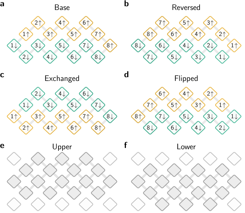
Refer to caption
Figure S8: Various qubit assignments of the 1D Fermi-Hubbard model on a 23-qubit grid. a. The original configuration is used as the base. We generate new configurations by applying the following operations and their combinations on the base: b. reversing the sites, c. exchanging the spin states, d. flipping the sites horizontally. Each configuration can either take one of the two subsets of the grid: e. the upper part, f. the lower part. This leads to 161616 different qubit assignments. The same assignments are used regardless if interaction terms are present (U0𝑈0U\neq 0) or not (U=0𝑈0U=0).
Refer to caption
Figure S9: The damping factor (scale): a. the U=0𝑈0U=0 and NP=2subscript𝑁𝑃2N_{P}=2 case in Fig. 3, b. the U=2𝑈2U=2 and NP=4subscript𝑁𝑃4N_{P}=4 case in Fig. 2. The data points are obtained by comparing the numerical and experimental results at each Trotter step. The shaded areas represent the standard errors of regression and the solid lines represent the linear fittings of the data points. The bottom plots show the effectiveness of the rescaling procedure using the linear relation in Eq. (3): a. center of mass positions of the spin-up (yellow and orange) and spin-down (green and purple) states, b. spreads of the two spin states.
Refer to caption
Figure S10: T1subscript𝑇1T_{1} relaxation times ( µstimesabsentmicrosecond\text{\,}\mathrm{\SIUnitSymbolMicro s}) at idle frequencies.
Refer to caption
Figure S11: Two-qubit gate percent Pauli error obtained by cross-entropy benchmarking (XEB), where non-conflicting subsets of two-qubit gates are applied simultaneously. These values were measured against the standard iSWAPsuperscriptiSWAP\sqrt{\mbox{\footnotesize{iSWAP}}}^{\,{\dagger}} without the parasitic controlled phases. The two-qubit gates are calibrated using our routine calibration process without Floquet calibration, see Section V in the Supplementary information in [arute_quantum_2019].
Refer to caption
(a)
Figure S12: Detailed data for the N=N=2subscript𝑁subscript𝑁2N_{\uparrow}=N_{\downarrow}=2 case. a. Charge and spin densities ρj±superscriptsubscript𝜌𝑗plus-or-minus\rho_{j}^{\pm} as functions of the site numbers at different evolution times for interaction strengths u=0,1.5,3,4.5𝑢01.534.5u=0,1.5,3,4.5. b. Charge and spin spread κ±superscript𝜅plus-or-minus\kappa^{\pm} and their derivatives as functions of time for different values of u𝑢u.
Refer to caption
(a)
Figure S13: Detailed data for the N=N=3subscript𝑁subscript𝑁3N_{\uparrow}=N_{\downarrow}=3 case. a. Charge and spin densities ρj±superscriptsubscript𝜌𝑗plus-or-minus\rho_{j}^{\pm} as functions of the site numbers at different evolution times for interaction strengths u=0,1.5,3,4.5𝑢01.534.5u=0,1.5,3,4.5. b. Charge and spin spread κ±superscript𝜅plus-or-minus\kappa^{\pm} and their derivatives for different values of u𝑢u.