Achievable Rate Region and Path-Based Beamforming for Multi-User Single-Carrier
Delay Alignment Modulation

Abstract

Delay alignment modulation (DAM) is a novel wideband transmission technique for millimeter wave (mmWave) massive multiple-input multiple-output (MIMO) systems, which exploits the high spatial resolution and multi-path sparsity to mitigate inter-symbol interference (ISI), without relying on channel equalization or multi-carrier transmission. In particular, DAM leverages the delay pre-compensation and path-based beamforming to effectively align the multi-path components, thus achieving the constructive multi-path combination for eliminating the ISI while preserving the multi-path power gain. Different from the existing works only considering single-user DAM, this paper investigates the DAM technique for multi-user mmWave massive MIMO communication. First, we consider the asymptotic regime when the number of antennas $M_{t}$ at base station (BS) is sufficiently large. It is shown that by employing the simple delay pre-compensation and per-path-based maximal ratio transmission (MRT) beamforming, the single-carrier DAM is able to perfectly eliminate both ISI and inter-user interference (IUI). Next, we consider the general scenario with $M_{t}$ being finite. In this scenario, we characterize the achievable rate region of the multi-user DAM system by finding its Pareto boundary. Specifically, we formulate a rate-profile-constrained sum rate maximization problem by optimizing the per-path-based beamforming, which is optimally solved via the second-order cone programming (SOCP). Furthermore, we present three low-complexity per-path-based beamforming strategies based on the MRT, zero-forcing (ZF), and regularized zero-forcing (RZF) principles, respectively, based on which the achievable sum rates are studied. Finally, we provide simulation results to demonstrate the performance of our proposed strategies as compared to two benchmark schemes based on the strongest-path-based beamforming and the prevalent orthogonal frequency division multiplexing (OFDM), respectively. It is shown that DAM achieves higher spectral efficiency and/or lower peak-to-average-ratio (PAPR), for systems with high spatial resolution and multi-path diversity.

I Introduction

Recently, delay alignment modulation (DAM) was proposed as a novel technique to tackle the inter-symbol interference (ISI) issue in wideband communication systems, without relying on channel equalization or multi-carrier transmissions [2]. DAM is particularly appealing for systems with large antenna arrays [3, 4] and high-frequency bands such as millimeter wave (mmWave) [5] and Terahertz (THz) systems, which have the super spatial resolution and multi-path sparsity. In particular, by manipulating the channel delay spread via delay pre-compensation and path-based beamforming, DAM enables all multi-path signal components to reach the receiver concurrently and constructively, thus eliminating the detrimental ISI while preserving the multi-path channel power gains. This renders DAM resilient to time-dispersive channels for efficient single- and multi-carrier transmissions. There have been some preliminary works on DAM in the literature [6, 7, 8, 9, 10]. For example, by combining DAM with orthogonal frequency division multiplexing (OFDM), a novel DAM-OFDM scheme was proposed in [7], which provides a unified framework to achieve ISI-free communication using single- or multi-carrier transmissions by flexibly manipulating the channel delay spread and the number of sub-carriers. Furthermore, DAM was exploited for integrated sensing and communication (ISAC) and multi-intelligent reflecting surfaces (IRSs) aided communication in [8], [9] and [10], respectively.

DAM is significantly different from existing ISI-mitigation techniques, such as channel equalization, spread spectrum, and multi-carrier transmission. First, channel equalization can be generally classified into time- and frequency-domain equalization, respectively. For time-domain equalization, a particular time reversal (TR) for single-carrier transmission was proposed in [11] by treating the multi-path channel as an intrinsic matched filter [11, 12], in which the ISI issue is addressed by compromising the communication rate due to the use of rate back-off technique. In [13] and [14], channel shortening technique was proposed by applying a time-domain finite impulse response (FIR) filter, in which the effective channel impulse response is shortened to avoid long cyclic prefix (CP). However, the time-domain equalization needs a large number of taps for systems with large channel delay spread. Besides time-domain equalization, frequency-domain equalization reduces the signal processing complexity by converting the signal to the frequency-domain via discrete Fourier transform (DFT) [14], [15]. By contrast, DAM can completely eliminate ISI via spatial-delay processing. Spread spectrum techniques like RAKE receiver [16] require spread spectrum codes with good auto/cross-correlation and bandwidth expansion, i.e., using bandwidth much larger than necessary for data transmission, while DAM avoids these issues. In addition, OFDM and OTFS are two widely adopted multi-carrier communication technologies. OFDM suffers from practical issues like sensitivity to carrier frequency offset (CFO), high peak-to-average-power ratio (PAPR), and the severe out-of-band (OOB) emission [16]. Moreover, orthogonal time-frequency space (OTFS) modulation was recently proposed by modulating information in the delay-Doppler domain, which shows superior performance to OFDM in high mobility scenarios [17]. However, the multi-carrier OTFS technique has high complexity when extending to massive MIMO systems [18]. In addition, OTFS in general needs to perform signal detection across the entire OTFS frame, thus leading to a high detection delay. By contrast, as a spatial-delay processing technique, DAM is expected to overcome the aforementioned issues. For example, compared to OFDM and OTFS, single-carrier DAM enables the instant symbol-by-symbol signal detection at the receiver [10].

DAM is also different from various delay pre-compensation techniques in [19, 20, 21, 22]. For example, unlike DAM, [19] and [20] did not exploit the high spatial resolution or multi-path sparsity of mmWave massive MIMO systems to eliminate ISI. In addition, for mmWave MIMO systems, [21] and [22] were designed for the special lens MIMO or hybrid beamforming architectures, respectively. Besides, equalization-free single-carrier modulation was also advocated in [23] and [24], where beam alignment along the single dominant path was applied to transform the time-variant frequency-selective channel into time-invariant frequency-flat channel [23]. Furthermore, the measurement campaign in [24] showed that little or no equalization is needed with such a beam alignment scheme. However, both [23] and [24] only treat the single dominant path as the desired signal and all other multi-path signal as noise, while DAM makes full use of all multipath channel components and hence a better performance is expected, as demonstrated in the simulation results later.

Note that existing works on DAM [2], [6, 9, 7, 8, 10] only consider the single-user scenario. In this paper, we study the more general multi-user DAM systems. In contrast to single-user DAM that only addresses the ISI issue, multi-user DAM design needs to handle both the ISI and inter-user interference (IUI). The main contributions of this paper are summarized as follows:

• First, to gain essential insights, we provide an asymptotic analysis by assuming that the number of BS antennas $M_{t}$ is sufficiently large. In this case, we show that with the low-complexity delay pre-compensation and per-path-based MRT beamforming, the multi-user time-dispersive broadcast channel with ISI and IUI can be transformed into ISI-free and IUI-free additive white Gaussian noise (AWGN) channels.

• Second, for the general scenario with a finite number of BS antennas, we characterize the achievable rate region of the multi-user DAM system by finding its Pareto boundary. The rate-profile-constrained sum rate maximization problem is formulated by optimizing the per-path-based beamforming, which is optimally solved via second-order cone programming (SOCP).

• Third, we present three low-complexity beamforming strategies in a per-path basis, namely MRT, zero-forcing (ZF), and regularized zero-forcing (RZF), respectively. Specifically, low complexity per-path-based MRT beamforming for multi-user DAM with tolerable ISI and IUI is firstly developed. Then, when $M_{t}\geq L_{\mathrm{tot}}$, both the ISI and IUI are completely eliminated with the per-path-based ZF beamforming, and the optimal power allocation for sum rate maximization is obtained. Furthermore, the more general per-path-based RZF beamforming with tolerable ISI and IUI is developed to balance the noise enhancement in the ZF beamforming and the interference limitation in the MRT beamforming.

• Last, we compare the proposed multi-user single-carrier DAM designs with two benchmarking schemes, i.e., the alternative single-carrier ISI suppression technique that only uses the strongest channel path of each user and the prevalent OFDM scheme. Extensive simulation results are provided to demonstrate the advantages of single-carrier DAM over the benchmarking schemes, in terms of spectral efficiency and/or PAPR.

The rest of this paper is organized as follows. Section II presents the system model and provides the asymptotic analysis when $M_{t}$ is sufficiently large. Section III characterizes the achievable rate region for multi-user DAM. Section IV studies the sum rate for multi-user DAM. Section V compares the multi-user DAM against the benchmarking schemes of strongest-path-based beamforming and OFDM. Section VI presents numerical results. Finally, we conclude the paper in Section VII.

Notations: Scalars are denoted by italic letters. Vectors and matrices are denoted by boldface lower- and upper-case letters, respectively. For a matrix $\boldsymbol{\bf{A}}\in\mathbb{C}^{M\times N}$, $\boldsymbol{\bf{A}}^{T},\boldsymbol{\bf{A}}^{H},\boldsymbol{\bf{A}}^{\dagger}$, $\|\boldsymbol{\bf{A}}\|_{F}$, $\Im(\boldsymbol{\bf{A}})$, and $\Re(\boldsymbol{\bf{A}})$ denote its transpose, Hermitian transpose, pseudo-inverse, Frobenius norm, imaginary part, and real part, respectively. For a vector $\boldsymbol{\bf{a}}$, $\|\boldsymbol{\bf{a}}\|$ denotes the $l_{2}$-norm. $\mathbb{E}[\cdot]$, $\delta[\cdot]$, $\max[\cdot]$, and $\min[\cdot]$ denote the expectation, Dirac-delta impulse function, maximum and minimum operators, respectively. $*$, and $\mathcal{CN}(\boldsymbol{\bf{x}},\boldsymbol{\bf{\Sigma}})$ denote linear convolution, and circularly symmetric complex Gaussian (CSCG) distribution of a random vector with mean vector $\boldsymbol{\bf{x}}$ and covariance matrix $\boldsymbol{\bf{\Sigma}}$, respectively, and $(a)^{+}\triangleq\max(a,0)$.

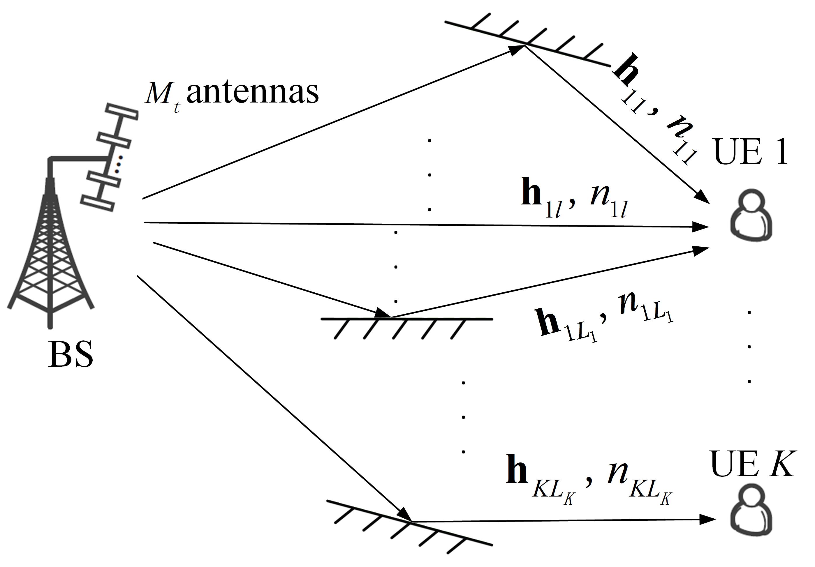
Figure 1: A multi-user mmWave massive MIMO communication system in time-dispersive channels.

II System Model and Asymptotic Analysis

As shown in Fig. 1, we consider a multi-user mmWave massive MIMO communication system, where the BS equipped with $M_{t}\gg 1$ antennas serves $K$ single-antenna user equipments (UEs). In time-dispersive multi-path environment, the baseband discrete-time channel impulse response of UE $k$ within one channel coherence block is expressed as

$$\boldsymbol{\bf{h}}_{k}[n]=\sum_{l=1}^{L_{k}}\boldsymbol{\bf{h}}_{kl}\delta[n-n_{kl}],$$ (1)

where $\boldsymbol{\bf{h}}_{kl}\in\mathbb{C}^{M_{t}\times 1}$ denotes the channel coefficient vector for the $l$th multi-path of UE $k$, $L_{k}$ is the number of temporal-resolvable multi-paths of UE $k$, and $n_{kl}$ denotes its discretized delay, with $n_{kl}\neq n_{kl^{\prime}},\forall l^{\prime}\neq l$. Let $n_{k,\text{max}}=\max\limits_{1\leq l\leq L_{k}}n_{kl}$ and $n_{k,\text{min}}=\min\limits_{1\leq l\leq L_{k}}n_{kl}$ denote the maximum and minimum delays of UE $k$, respectively.

Let $s_{k}[n]$ denote the independent and identically distributed (i.i.d.) information-bearing symbols of UE $k$ with normalized power $\mathbb{E}[|s_{k}[n]|^{2}]=1$. By extending the DAM technique proposed in [2] to multi-user systems, the transmitted signal by the BS for multi-user single-carrier DAM is

$$\boldsymbol{\bf{x}}[n]=\sum_{k=1}^{K}\sum_{l^{\prime}=1}^{L_{k}}\boldsymbol{\bf{f}}_{kl^{\prime}}s_{k}[n-\kappa_{kl^{\prime}}],$$ (2)

where $\boldsymbol{\bf{f}}_{kl^{\prime}}\in\mathbb{C}^{M_{t}\times 1}$ denotes the per-path-based transmit beamforming vector associated with multi-path $l^{\prime}$ of UE $k$, and $\kappa_{kl^{\prime}}$ is the deliberately introduced delay pre-compensation, with $\kappa_{kl^{\prime}}=n_{k,\text{max}}-n_{kl^{\prime}}\geq 0,\forall l^{\prime}=1,...,L_{k}$. Since $\{n_{kl^{\prime}},\forall k,l^{\prime}\}$ are distinct for different paths $l^{\prime}$, we have $\kappa_{kl^{\prime}}\neq\kappa_{kl}$, $\forall l^{\prime}\neq l$. The block diagram of multi-user single-carrier DAM is illustrated in Fig. 2. By using the fact that $s_{k}[n]$ is independent across different $n$ and $k$ as well as $\kappa_{kl^{\prime}}\neq\kappa_{kl},\forall l\neq l^{\prime}$, the transmit power of the BS is

$$\mathbb{E}[\|\boldsymbol{\bf{x}}[n]\|^{2}]=\begin{matrix}\sum_{k=1}^{K}\end{matrix}\begin{matrix}\sum_{l^{\prime}=1}^{L_{k}}\end{matrix}\|\boldsymbol{\bf{f}}_{kl^{\prime}}\|^{2}\leq P,$$ (3)

where $P$ is the maximum allowable transmit power.

Based on (1) and (2), the received signal at UE $k$ for multi-user DAM system is

$$y_{k}[n]=\boldsymbol{\bf{h}}_{k}^{H}[n]*\boldsymbol{\bf{x}}[n]+z_{k}[n]$$ (4)

$$=\underbrace{\left(\begin{matrix}\sum_{l=1}^{L_{k}}\end{matrix}\boldsymbol{\bf{h}}_{kl}^{H}\boldsymbol{\bf{f}}_{kl}\right)s_{k}[n-n_{k,\text{max}}]}_{\text{Desired signal}}$$

$$+\underbrace{\begin{matrix}\sum_{l=1}^{L_{k}}\end{matrix}\begin{matrix}\sum_{l^{\prime}\neq l}^{L_{k}}\end{matrix}\boldsymbol{\bf{h}}_{kl}^{H}\boldsymbol{\bf{f}}_{kl^{\prime}}s_{k}[n-n_{k,\text{max}}-n_{kl}+n_{kl^{\prime}}]}_{\text{ISI}}$$

$$+\underbrace{\sum_{l=1}^{L_{k}}\sum_{k^{\prime}\neq k}^{K}\sum_{l^{\prime}=1}^{L_{k^{\prime}}}\boldsymbol{\bf{h}}_{kl}^{H}\boldsymbol{\bf{f}}_{k^{\prime}l^{\prime}}s_{k^{\prime}}[n-n_{k^{\prime},\text{max}}-n_{kl}+n_{k^{\prime}l^{\prime}}]}_{\text{IUI}}+z_{k}[n],$$

where $z_{k}[n]\sim\mathcal{CN}(0,\sigma^{2})$ denotes the AWGN at UE $k$. It is observed that when UE $k$ performs the simple single-tap detection for signal with delay $n_{k,\text{max}}$, then the first term is the desired signal, and the second and third terms are the ISI and IUI, respectively.

To show the benefit of DAM in multi-user mmWave massive MIMO, we first provide the asymptotic analysis by considering that the number of BS antennas $M_{t}$ is much larger than the total number of temporal-resolvable multi-paths $L_{\mathrm{tot}}=\sum_{k=1}^{K}L_{k}$. We will show that in this special scenario, both the ISI and IUI in (4) asymptotically vanish with the simple per-path-based MRT beamforming.

First, we consider the correlation property of the channel vectors $\boldsymbol{\bf{h}}_{kl},k=1,...,K,l=1,...,L_{k}$. Based on the asymptotic analysis in [7], it was shown that as long as the multi-paths correspond to distinct angle-of-departures (AoDs), the channel vectors of different multi-path delays are asymptotically orthogonal when $M_{t}\gg L_{\mathrm{tot}}$, i.e.,

$$\lim_{M_{t}\to\infty}\frac{|\boldsymbol{\bf{h}}_{kl}^{H}\boldsymbol{\bf{h}}_{k^{\prime}l^{\prime}}|}{\|\boldsymbol{\bf{h}}_{kl}\|~{}\|\boldsymbol{\bf{h}}_{k^{\prime}l^{\prime}}\|}\to 0,\forall k^{\prime}\neq k,\text{or}~{}l^{\prime}\neq l.$$ (5)

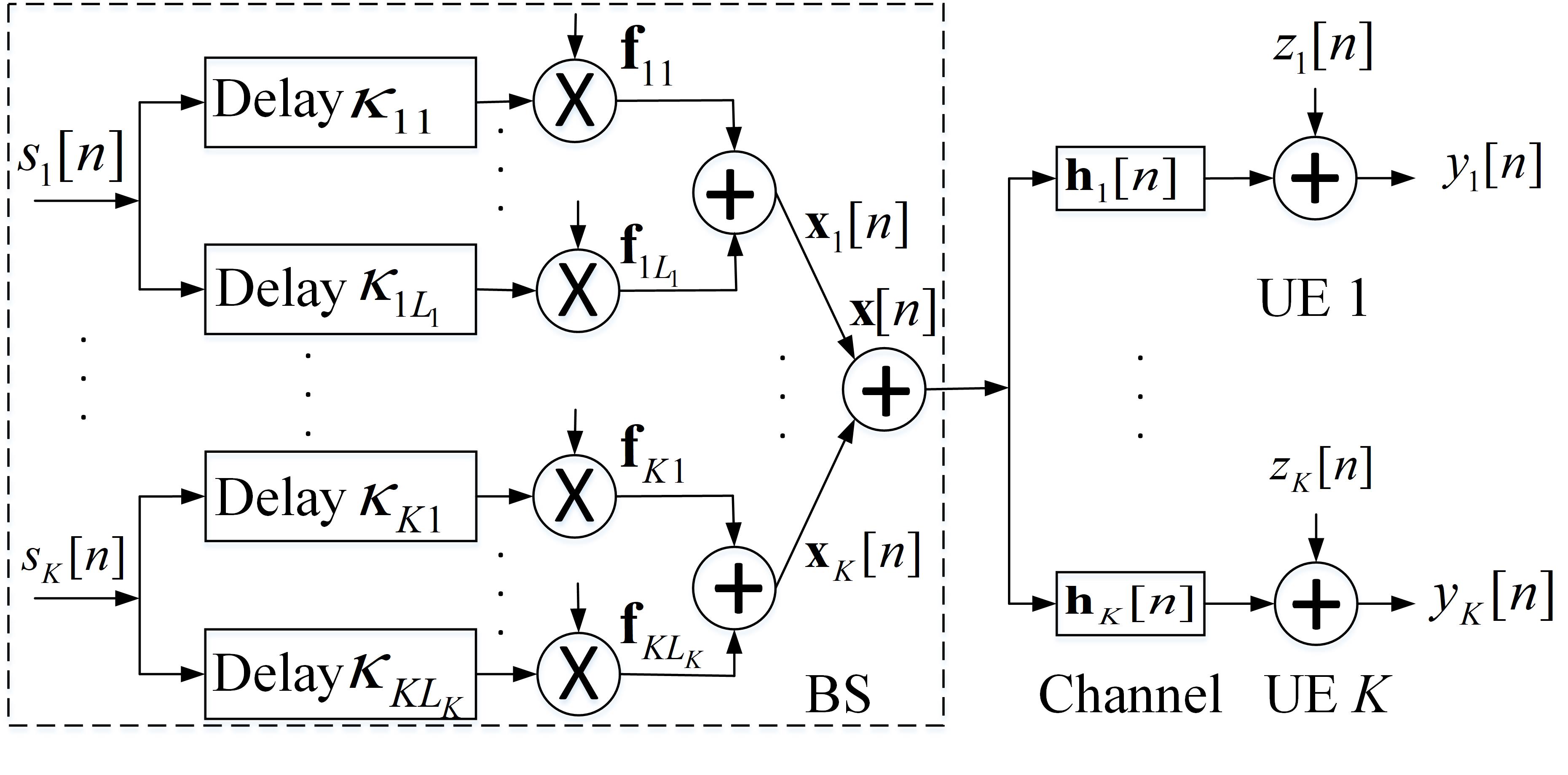
Figure 2: Block diagram for multi-user single-carrier DAM.

By exploiting the above asymptotically orthogonal property, the ISI and IUI in (4) for the single-carrier DAM system can be eliminated by the low-complexity per-path-based MRT beamforming. With MRT, the per-path-based beamforming vectors in (2) are set as

$$\boldsymbol{\bf{f}}_{kl^{\prime}}=\xi_{k}\sqrt{p_{k}}\boldsymbol{\bf{h}}_{kl^{\prime}},k=1,...,K,l^{\prime}=1,...L_{k},$$ (6)

where $\xi_{k}=1/\sqrt{\sum_{j=1}^{L_{k}}\|\boldsymbol{\bf{h}}_{kj}\|^{2}}$ is the normalization factor and $p_{k}$ denotes the transmit power allocated to UE $k$. In this case, by scaling the signal in (4) with $\xi_{k}$, we have

$$\xi_{k}y_{k}[n] =\sqrt{p_{k}}s_{k}[n-n_{k,\text{max}}]+\sqrt{p_{k}}\sum_{l=1}^{L_{k}}\sum_{l^{\prime}\neq l}^{L_{k}}\frac{\boldsymbol{\bf{h}}_{kl}^{H}\boldsymbol{\bf{h}}_{kl^{\prime}}}{\sum_{j=1}^{L_{k}}\|\boldsymbol{\bf{h}}_{kj}\|^{2}}$$

$$\times s_{k}[n-n_{k,\text{max}}-n_{kl}+n_{kl^{\prime}}]$$

$$+\sum_{l=1}^{L_{k}}\sum_{k^{\prime}\neq k}^{K}\sum_{l^{\prime}=1}^{L_{k^{\prime}}}\frac{\sqrt{p_{k^{\prime}}}\boldsymbol{\bf{h}}_{kl}^{H}\boldsymbol{\bf{h}}_{k^{\prime}l^{\prime}}}{\sqrt{\sum_{j=1}^{L_{k}}\|\boldsymbol{\bf{h}}_{kj}\|^{2}}~{}\sqrt{\sum_{j=1}^{L_{k^{\prime}}}\|\boldsymbol{\bf{h}}_{k^{\prime}j}\|^{2}}}$$

$$\times s_{k^{\prime}}[n-n_{k^{\prime},\text{max}}-n_{kl}+n_{k^{\prime}l^{\prime}}]+\xi_{k}z_{k}[n].$$ (7)

Thanks to the asymptotically orthogonal property in (5), when $M_{t}\gg L_{\mathrm{tot}}$, we have

$$\frac{|\boldsymbol{\bf{h}}_{kl}^{H}\boldsymbol{\bf{h}}_{kl^{\prime}}|}{\sum_{j=1}^{L_{k}}\|\boldsymbol{\bf{h}}_{kj}\|^{2}}\leq\frac{|\boldsymbol{\bf{h}}_{kl}^{H}\boldsymbol{\bf{h}}_{kl^{\prime}}|}{\|\boldsymbol{\bf{h}}_{kl}\|^{2}+\|\boldsymbol{\bf{h}}_{kl^{\prime}}\|^{2}}\leq\frac{|\boldsymbol{\bf{h}}_{kl}^{H}\boldsymbol{\bf{h}}_{kl^{\prime}}|}{\|\boldsymbol{\bf{h}}_{kl}\|~{}\|\boldsymbol{\bf{h}}_{kl^{\prime}}\|}\to 0,$$ (8)

and

$$\begin{split}&\frac{|\boldsymbol{\bf{h}}_{kl}^{H}\boldsymbol{\bf{h}}_{k^{\prime}l^{\prime}}|}{\sqrt{(\sum_{j=1}^{L_{k}}\|\boldsymbol{\bf{h}}_{kj}\|^{2})(\sum_{j=1}^{L_{k^{\prime}}}\|\boldsymbol{\bf{h}}_{k^{\prime}j}\|^{2})}}\\ &\leq\frac{|\boldsymbol{\bf{h}}_{kl}^{H}\boldsymbol{\bf{h}}_{k^{\prime}l^{\prime}}|}{\sqrt{\|\boldsymbol{\bf{h}}_{kl}\|^{2}~{}\|\boldsymbol{\bf{h}}_{k^{\prime}l^{\prime}}\|^{2}}}=\frac{|\boldsymbol{\bf{h}}_{kl}^{H}\boldsymbol{\bf{h}}_{k^{\prime}l^{\prime}}|}{\|\boldsymbol{\bf{h}}_{kl}\|~{}\|\boldsymbol{\bf{h}}_{k^{\prime}l^{\prime}}\|}\to 0.\end{split}$$ (9)

Based on (8) and (9), and by dividing both sides of (II) with $\xi_{k}$, the resulting signal for UE $k$ reduces to

$$y_{k}[n]\to\sqrt{p_{k}\sum_{j=1}^{L_{k}}\|\boldsymbol{\bf{h}}_{kj}\|^{2}}s_{k}[n-n_{k,\text{max}}]+z_{k}[n],k=1,...,K.$$ (10)

It follows from (10) that for multi-user single-carrier DAM with the simple delay pre-compensation and per-path-based MRT beamforming, the resulting signal of UE $k$ only includes the desired symbol sequence $s_{k}[n]$ with one single delay $n_{k,\text{max}}$, while still achieving the channel gain contributed by all the $L_{k}$ paths. As a result, the original time-dispersive multi-user channels with both ISI and IUI have been transformed to $K$ parallel ISI-free and IUI-free AWGN channels, without relying on the conventional techniques like channel equalization or multi-carrier transmission. Moreover, based on the received signal in (10), the resulting signal-to-noise ratio (SNR) at UE $k$ is given by $\gamma_{k}^{\text{asym}}=p_{k}{\|\bar{\boldsymbol{\bf{h}}}_{k}\|^{2}}/{\sigma^{2}}$, where $\bar{\boldsymbol{\bf{h}}}_{k}=[\boldsymbol{\bf{h}}_{k1}^{H},...,\boldsymbol{\bf{h}}_{kL_{k}}^{H}]^{H}\in\mathbb{C}^{M_{t}L_{k}\times 1}$. In this case, the optimal power allocation across UEs to maximize the asymptotic sum rate of all the $K$ UEs is readily obtained by the classical water-filling (WF) strategy [16].

In the following, we investigate the performance of multi-user DAM when the BS is equipped with a finite number of antennas. The optimal rate region and the achievable sum rate with classical beamforming strategies are analyzed and compared with benchmarking schemes.

III Rate Region for Multi-User DAM with Optimal Beamforming

III-A Achievable Rate Region with Optimal Beamforming

To characterize the achievable rate region for the multi-user DAM system, we first derive the signal-to-interference-plus-noise ratio (SINR) for the received signal in (4), by treating the ISI and IUI as noise. Since the ISI and IUI in (4) may have correlated terms, the symbols need to be properly grouped by considering the delay differences of the signal components [2]. To this end, let $\Delta_{kl,k^{\prime}l^{\prime}}=n_{kl}-n_{k^{\prime}l^{\prime}}$ denote the delay difference between multi-path $l$ of UE $k$ and multi-path $l^{\prime}$ of UE $k^{\prime}$. For a given UE pair $(k,k^{\prime})$, we have $\Delta_{kl,k^{\prime}l^{\prime}}\in\{\Delta_{kk^{\prime},\min},\Delta_{kk^{\prime},\min}+1,...,\Delta_{kk^{\prime},\max}\}$, where $\Delta_{kk^{\prime},\min}=n_{k,\text{min}}-n_{k^{\prime},\text{max}}$ and $\Delta_{kk^{\prime},\max}=n_{k,\text{max}}-n_{k^{\prime},\text{min}}$. Then for each UE pair $(k,k^{\prime})$ and delay difference $i\in\{\Delta_{kk^{\prime},\min},\Delta_{kk^{\prime},\min}+1,...,\Delta_{kk^{\prime},\max}\}$, we define the following effective channel

$$\boldsymbol{\bf{g}}_{kk^{\prime}l^{\prime}}[i]=\begin{cases}\boldsymbol{\bf{h}}_{kl},&\text{if}~{}\exists l\in\{1,...,L_{k}\},~{}\mbox{s.t.}~{}\Delta_{kl,k^{\prime}l^{\prime}}=i,\\ \boldsymbol{\bf{0}},&\mbox{otherwise}.\end{cases}$$ (11)

Then, the received signal in (4) is equivalently rewritten as

$$y_{k}[n]={\left(\begin{matrix}\sum_{l=1}^{L_{k}}\end{matrix}\boldsymbol{\bf{h}}_{kl}^{H}\boldsymbol{\bf{f}}_{kl}\right)s_{k}[n-n_{k,\text{max}}]}$$ (12)

$$+{\sum_{i=\Delta_{kk,\min},i\neq 0}^{\Delta_{kk,\max}}\left(\sum_{l^{\prime}=1}^{L_{k}}\boldsymbol{\bf{g}}_{kkl^{\prime}}^{H}[i]\boldsymbol{\bf{f}}_{kl^{\prime}}\right)s_{k}[n-n_{k,\text{max}}-i]}$$

$$+{\sum_{k^{\prime}\neq k}^{K}\sum_{i=\Delta_{kk^{\prime},\min}}^{\Delta_{kk^{\prime},\max}}\left(\sum_{l^{\prime}=1}^{L_{k^{\prime}}}\boldsymbol{\bf{g}}_{kk^{\prime}l^{\prime}}^{H}[i]\boldsymbol{\bf{f}}_{k^{\prime}l^{\prime}}\right)s_{k^{\prime}}[n-n_{k^{\prime},\text{max}}-i]}$$

$$+z_{k}[n].$$

$$\begin{split}\gamma_{k}&=\frac{|\sum_{l=1}^{L_{k}}\boldsymbol{\bf{h}}_{kl}^{H}\boldsymbol{\bf{f}}_{kl}|^{2}}{\sum_{i=\Delta_{kk,\min},i\neq 0}^{\Delta_{kk,\max}}|\sum_{l^{\prime}=1}^{L_{k}}\boldsymbol{\bf{g}}_{kkl^{\prime}}^{H}[i]\boldsymbol{\bf{f}}_{kl^{\prime}}|^{2}+\sum_{k^{\prime}\neq k}^{K}\sum_{i=\Delta_{kk^{\prime},\min}}^{\Delta_{kk^{\prime},\max}}|\sum_{l^{\prime}=1}^{L_{k^{\prime}}}\boldsymbol{\bf{g}}_{kk^{\prime}l^{\prime}}^{H}[i]\boldsymbol{\bf{f}}_{k^{\prime}l^{\prime}}|^{2}+\sigma^{2}}\\ &=\frac{|\bar{\boldsymbol{\bf{h}}}_{k}^{H}\bar{\boldsymbol{\bf{f}}}_{k}|^{2}}{\sum_{i=\Delta_{kk,\min},i\neq 0}^{\Delta_{kk,\max}}|\bar{\boldsymbol{\bf{g}}}_{kk}^{H}[i]\bar{\boldsymbol{\bf{f}}}_{k}|^{2}+\sum_{k^{\prime}\neq k}^{K}\sum_{i=\Delta_{kk^{\prime},\min}}^{\Delta_{kk^{\prime},\max}}|\bar{\boldsymbol{\bf{g}}}_{kk^{\prime}}^{H}[i]\bar{\boldsymbol{\bf{f}}}_{k^{\prime}}|^{2}+\sigma^{2}}\\ &=\frac{|\bar{\boldsymbol{\bf{h}}}_{k}^{H}\bar{\boldsymbol{\bf{f}}}_{k}|^{2}}{||\boldsymbol{\bf{G}}_{kk}^{H}\bar{\boldsymbol{\bf{f}}}_{k}||^{2}+\sum_{k^{\prime}\neq k}^{K}||\boldsymbol{\bf{G}}_{kk^{\prime}}^{H}\bar{\boldsymbol{\bf{f}}}_{k^{\prime}}||^{2}+\sigma^{2}}.\end{split}$$ (13)

The resulting SINR is given in (13), shown at the top of the next page, where we have defined:

$$\bar{\boldsymbol{\bf{f}}}_{k} \triangleq[\boldsymbol{\bf{f}}_{k1}^{H},...,\boldsymbol{\bf{f}}_{kL_{k}}^{H}]^{H}\in\mathbb{C}^{M_{t}L_{k}\times 1},$$ (14)

$$\bar{\boldsymbol{\bf{g}}}_{kk^{\prime}}[i] \triangleq\Big{[}\boldsymbol{\bf{g}}_{kk^{\prime}1}^{H}[i],...,\boldsymbol{\bf{g}}_{kk^{\prime}L_{k^{\prime}}}^{H}[i]\Big{]}^{H}\in\mathbb{C}^{M_{t}L_{k^{\prime}}\times 1},$$ (15)

$$\boldsymbol{\bf{G}}_{kk^{\prime}} \triangleq\Big{[}\bar{\boldsymbol{\bf{g}}}_{kk^{\prime}}[\Delta_{kk^{\prime},\min}],...,\bar{\boldsymbol{\bf{g}}}_{kk^{\prime}}[\Delta_{kk^{\prime},\max}]\Big{]},$$ (16)

with $\boldsymbol{\bf{G}}_{kk^{\prime}}\in\mathbb{C}^{M_{t}L_{k^{\prime}}\times{\Delta_{kk^{\prime},\text{span}}}}$, and $\Delta_{kk^{\prime},\text{span}}=\Delta_{kk^{\prime},\max}-\Delta_{kk^{\prime},\min}$.

Therefore, with the per-path-based transmit beamforming vectors $(\bar{\boldsymbol{\bf{f}}}_{1},...,\bar{\boldsymbol{\bf{f}}}_{K})$, the achievable rate for UE $k$ is $R_{k}(\bar{\boldsymbol{\bf{f}}}_{1},...,\bar{\boldsymbol{\bf{f}}}_{K})=\text{log}_{2}(1+\gamma_{k})$, and the achievable rate region is the union of all rate-tuples that is achieved by the $K$ users, given by

$$\mathcal{R}\triangleq\bigcup_{\sum_{k=1}^{K}||\bar{\boldsymbol{\bf{f}}}_{k}||^{2}\leq P}\left\{(r_{1},...,r_{K}):r_{k}=R_{k}(\bar{\boldsymbol{\bf{f}}}_{1},...,\bar{\boldsymbol{\bf{f}}}_{K}),\forall k\right\}.$$ (17)

The outermost boundary of $\mathcal{R}$ is known as the Pareto boundary [25]. Similar to [25] and [26], the Pareto boundary of the rate region $\mathcal{R}$ can be obtained via solving the following optimization problem for a given set of rate-profile vectors, $\boldsymbol{\alpha}=(\alpha_{1},..,\alpha_{K})$:

$$\max\limits_{R,\{\bar{\boldsymbol{\bf{f}}}_{k}\}_{k=1}^{K}}~{} R$$ (18)

s.t. $$\text{log}_{2}(1+\gamma_{k})\geq\alpha_{k}R,~{}k=1,...,K,$$

$$\sum_{k=1}^{K}||\bar{\boldsymbol{\bf{f}}}_{k}||^{2}\leq P,$$

where $\alpha_{k}\geq 0,\forall k$ denotes the weighting coefficient for UE $k$, with $\sum_{k=1}^{K}\alpha_{k}=1$. For any given $\boldsymbol{\alpha}$, let $R^{\star}$ denote optimal value to problem (18). Then the rate-tuple $R^{\star}\boldsymbol{\alpha}$ is the intersection between the Pareto boundary of the rate region $\mathcal{R}$ and a ray in the direction of $\boldsymbol{\alpha}$. After solving problem (18) with different rate-profile vectors $\boldsymbol{\alpha}$, the complete Pareto boundary of $\mathcal{R}$ can be found.

To solve problem (18) with any given rate-profile vector $\boldsymbol{\alpha}$ and target rate $R$, it can be transformed into the feasibility problem, given by

Find $$\bar{\boldsymbol{\bf{f}}}_{1},...,\bar{\boldsymbol{\bf{f}}}_{K}$$ (19)

s.t. $$\text{log}_{2}(1+\gamma_{k})\geq\alpha_{k}R,~{}k=1,...,K,$$

$$\sum_{k=1}^{K}||\bar{\boldsymbol{\bf{f}}}_{k}||^{2}\leq P.$$

Let $\gamma_{k}^{D}=2^{\alpha_{k}R}-1$, we consider the following problem to minimize the BS transmit power, subject to the minimum SINR constraint for each UE, which is equivalent to problem (19), i.e.,

$$\min_{\{\bar{\boldsymbol{\bf{f}}}_{k}\}_{k=1}^{K}}~{} \sum_{k=1}^{K}||\bar{\boldsymbol{\bf{f}}}_{k}||^{2}$$ (20)

s.t. $$\Im{(\bar{\boldsymbol{\bf{h}}}_{k}^{H}\bar{\boldsymbol{\bf{f}}}_{k})}=0,~{}k=1,...,K,$$

$$\sqrt{\gamma_{k}^{D}}\begin{Vmatrix}\boldsymbol{\bf{G}}_{kk}^{H}\bar{\boldsymbol{\bf{f}}}_{k}\\ \boldsymbol{\bf{G}}_{k1}^{H}\bar{\boldsymbol{\bf{f}}}_{1}\\ ...\\ \boldsymbol{\bf{G}}_{k(k-1)}^{H}\bar{\boldsymbol{\bf{f}}}_{k-1}\\ \boldsymbol{\bf{G}}_{k(k+1)}^{H}\bar{\boldsymbol{\bf{f}}}_{k+1}\\ ...\\ \boldsymbol{\bf{G}}_{kK}^{H}\bar{\boldsymbol{\bf{f}}}_{K}\\ \sigma\end{Vmatrix}\leq\Re{(\bar{\boldsymbol{\bf{h}}}_{k}^{H}\bar{\boldsymbol{\bf{f}}}_{k})},k=1,...,K,$$

where without loss of optimality, we set $\bar{\boldsymbol{\bf{h}}}_{k}^{H}\bar{\boldsymbol{\bf{f}}}_{k}$ as a real number, since any common phase rotation to all elements in $\bar{\boldsymbol{\bf{f}}}_{k}$ does not alter the SINR $\gamma_{k}$ in (13) [27]. It is observed that problem (20) is a convex SOCP problem, which can be efficiently solved by standard convex optimization tools such as CVX [28]. If the obtained BS transmit power in problem (20) is no greater than $P$, then the optimal objective value of problem (18) satisfies $R^{\star}\geq R$; otherwise, $R^{\star}<R$. Thus, the original problem (18) can be solved by efficient bisection search over $R$, together with the SOCP problem (20) with given $R$. The key steps are summarized in Algorithm 1. Note that in Step 1, the upper bound $R_{U}$ is obtained by ignoring the ISI and IUI in (13), for which the beamforming vectors $\bar{\boldsymbol{\bf{f}}}_{k}$ simply matches with the channel $\bar{\boldsymbol{\bf{h}}}_{k}$.

In the following, for performance comparison, we study the achievable rate regions of two benchmarking schemes, namely the alternative single-carrier scheme termed strongest-path-based (SP) beamforming[19], which only exploits the single strongest path of each UE as the desired signal, and the multi-carrier OFDM scheme.

III-B Achievable Rate Region by the Strongest-Path-Based Beamforming

With the strongest-path-based beamforming, only a single beam is used for each user. Specifically, let $\boldsymbol{\bf{f}}_{k}\in\mathbb{C}^{M_{t}\times 1}$ denote the transmit beamforming vector of UE $k$. Then the transmitted signal

$$\boldsymbol{\bf{x}}_{\text{SP}}[n]=\sum_{k=1}^{K}\boldsymbol{\bf{f}}_{k}s_{k}[n].$$ (21)

Without loss of generality, we assume that the first path of each UE is the strongest path. Thus, with the channel model in (1), the received signal at UE $k$ for the strongest-path-based beamforming is expressed as

$$y_{k,\text{SP}}[n] =\boldsymbol{\bf{h}}_{k}^{H}[n]*\boldsymbol{\bf{x}}_{\text{SP}}[n]+{z}_{k}[n]$$ (22)

$$=\underbrace{\boldsymbol{\bf{h}}_{k1}^{H}\boldsymbol{\bf{f}}_{k}s_{k}[n-n_{k1}]}_{\text{Desired signal}}+\underbrace{\sum_{l\neq 1}^{L_{k}}\boldsymbol{\bf{h}}_{kl}^{H}\boldsymbol{\bf{f}}_{k}s_{k}[n-n_{kl}]}_{\text{ISI}}$$

$$+\underbrace{\sum_{l=1}^{L_{k}}\sum_{k^{\prime}\neq k}^{K}\boldsymbol{\bf{h}}_{kl}^{H}\boldsymbol{\bf{f}}_{k^{\prime}}s_{k^{\prime}}[n-n_{kl}]}_{\text{IUI}}+z_{k}[n].$$

In this case, only the single strongest path signal is regarded as the desired signal, and all the remaining $L_{\mathrm{tot}}-1$ multi-paths cause the detrimental ISI or IUI. The resulting SINR at UE $k$ based on (22) is

$$\gamma_{k}^{\text{SP}}=\frac{|\boldsymbol{\bf{h}}_{k1}^{H}\boldsymbol{\bf{f}}_{k}|^{2}}{\sum_{l\neq 1}^{L_{k}}|\boldsymbol{\bf{h}}_{kl}^{H}\boldsymbol{\bf{f}}_{k}|^{2}+\sum_{l=1}^{L_{k}}\sum_{k^{\prime}\neq k}^{K}|\boldsymbol{\bf{h}}_{kl}^{H}\boldsymbol{\bf{f}}_{k^{\prime}}|^{2}+\sigma^{2}}.$$ (23)

Note that when $M_{t}\gg L_{\mathrm{tot}}$, by applying MRT beamforming, with $\boldsymbol{\bf{f}}_{k}=\sqrt{\bar{p}_{k}}\frac{\boldsymbol{\bf{h}}_{k1}}{\|\boldsymbol{\bf{h}}_{k1}\|}$, where $\bar{p}_{k}$ is the power allocation of UE $k$, the received signal in (22) reduces to

$$y_{k,\text{SP}}[n]\to\sqrt{\bar{p}_{k}}\|\boldsymbol{\bf{h}}_{k1}\|s_{k}[n-n_{k1}]+z_{k}[n].$$ (24)

As compared with DAM, both ISI and IUI approach to zero asymptotically for the strongest-path-based beamforming, but the power for UE $k$ is only contributed by one single path, rather than all the $L_{k}$ multi-path as in DAM. The achievable rate region for the strongest-path-based beamforming can be similarly obtained with Algorithm 1 by replacing the SINR expression (13) as (23).

Algorithm 1 Solving Problem (18) to Find A Pareto-Optimal Point for Multi-User DAM Rate Region $\mathcal{R}$

1:Initialize: Set the lower bound $R_{L}=0$ and the upper bound $R_{U}=\min\limits_{k=1,...,K}\{R_{k}^{\star}/\alpha_{k}\}$, where $R_{k}^{\star}=\text{log}_{2}(1+P||\bar{\boldsymbol{\bf{h}}}_{k}||^{2}/\sigma^{2})$, and a small threshold $\epsilon$ and rate-profile vectors $\boldsymbol{\alpha}$.

2:while $(R_{U}-R_{L})>\epsilon R_{L}$ do

3:     Set $R=(R_{L}+R_{U})/2$;

4:     Solve the SOCP problem (20), and denote the optimal

5:     objective value as $P^{\star}$ and the resulting optimal

6:     solution as $\{\bar{\boldsymbol{\bf{f}}}_{k}\}_{k=1}^{K}$. If $P^{\star}\leq P$, then let $R_{L}=R$,

7:     and $\bar{\boldsymbol{\bf{f}}}_{k}^{\star}=\bar{\boldsymbol{\bf{f}}}_{k}$; otherwise, let $R_{U}=R$.

8:end while

9:$R^{\star}=R_{L}$ and $\{\bar{\boldsymbol{\bf{f}}}_{k}^{\star}\}_{k=1}^{K}$.

III-C Achievable Rate Region by OFDM

For the benchmarking OFDM scheme, let $M$ denote the number of sub-carriers. With the channel impulse response given in (1), the channel of the $m$th sub-carrier for UE $k$ can be obtained by applying $M$-point DFT, given by

$$\boldsymbol{\bf{h}}_{k,m}=\frac{1}{\sqrt{M}}\sum_{l=1}^{L_{k}}\boldsymbol{\bf{h}}_{kl}e^{-j\frac{2\pi mn_{kl}}{M}}.$$ (25)

The transmitted signal by the BS of the $m$th sub-carrier can be expressed as

$$\boldsymbol{\bf{x}}_{m}=\begin{matrix}\sum_{k=1}^{K}\end{matrix}\boldsymbol{\bf{d}}_{k,m}s_{k,m},$$ (26)

where $\boldsymbol{\bf{d}}_{k,m}\in\mathbb{C}^{M_{t}\times 1}$ and ${{s}}_{k,m}$ denote the frequency-domain beamforming vector and the information-bearing symbol for UE $k$ at the $m$th sub-carrier, respectively, with $\mathbb{E}[|s_{k,m}|^{2}]=1$. The corresponding power constraint is

$$\begin{matrix}\sum_{m=1}^{M}\end{matrix}\mathbb{E}[\|\boldsymbol{\bf{x}}_{m}\|^{2}]=\begin{matrix}\sum_{m=1}^{M}\end{matrix}\begin{matrix}\sum_{k=1}^{K}\end{matrix}\|\boldsymbol{\bf{d}}_{k,m}\|^{2}\leq MP.$$ (27)

After removing the cyclic prefix (CP) whose length is no smaller than the maximum delay spread of all UEs, the frequency-domain received signal of UE $k$ at the $m$th sub-carrier is

$$y_{k,m} =\boldsymbol{\bf{h}}_{k,m}^{H}\sum_{k^{\prime}=1}^{K}\boldsymbol{\bf{d}}_{k^{\prime},m}s_{k^{\prime},m}+{z}_{k,m}$$ (28)

$$=\underbrace{\boldsymbol{\bf{h}}_{k,m}^{H}\boldsymbol{\bf{d}}_{k,m}s_{k,m}}_{\text{Desired signal}}+\underbrace{\boldsymbol{\bf{h}}_{k,m}^{H}\begin{matrix}\sum_{k^{\prime}\neq k}^{K}\end{matrix}\boldsymbol{\bf{d}}_{k^{\prime},m}s_{k^{\prime},m}}_{\text{IUI}}+{z}_{k,m},$$

where ${z}_{k,m}\sim\mathcal{CN}(0,\hat{\sigma}^{2})$ is the AWGN with $\hat{\sigma}^{2}={\sigma^{2}}/{M}$. The corresponding SINR is expressed as

$$\gamma_{k,m}=\frac{|\boldsymbol{\bf{h}}_{k,m}^{H}\boldsymbol{\bf{d}}_{k,m}|^{2}}{\sum_{k^{\prime}\neq k}^{K}|\boldsymbol{\bf{h}}_{k,m}^{H}\boldsymbol{\bf{d}}_{k^{\prime},m}|^{2}+\hat{\sigma}^{2}}.$$ (29)

The achievable rate for UE $k$ without considering the CP overhead is thus $R_{k}=\frac{1}{M}\sum_{m=1}^{M}\text{log}_{2}(1+\gamma_{k,m})$. Similar to Section III-A, by using different rate-tuples $\boldsymbol{\bf{\alpha}}=(\alpha_{1},...,\alpha_{K})$, the Pareto boundary of the achievable rate region for OFDM can be obtained by solving the following optimization problem

$$\max\limits_{{\mu,\boldsymbol{\bf{d}}}_{k,m},\forall k,m}\mu$$ (30)

s.t. $$\sum_{m=1}^{M}\text{log}_{2}\bigg{(}1+\frac{|\boldsymbol{\bf{h}}_{k,m}^{H}\boldsymbol{\bf{d}}_{k,m}|^{2}}{\sum_{k^{\prime}\neq k}^{K}|\boldsymbol{\bf{h}}_{k,m}^{H}\boldsymbol{\bf{d}}_{k^{\prime},m}|^{2}+\hat{\sigma}^{2}}\bigg{)}\geq M\alpha_{k}\mu,\forall k,$$

$$\begin{matrix}\sum_{m=1}^{M}\end{matrix}\begin{matrix}\sum_{k=1}^{K}\end{matrix}||{\boldsymbol{\bf{d}}}_{k,m}||^{2}\leq MP.$$

Problem (30) is non-convex since the first constraint is non-convex. Fortunately, successive convex approximation (SCA) technique can be applied to obtain an efficient approximate solution [29]. To this end, problem (30) is equivalently written as

$$\max\limits_{{\mu,\boldsymbol{\bf{d}}}_{k,m},\forall k,m}\mu$$ (31)

s.t. $$\sum_{m=1}^{M}\text{log}_{2}\bigg{(}\sum_{k^{\prime}=1}^{K}|\boldsymbol{\bf{h}}_{k,m}^{H}\boldsymbol{\bf{d}}_{k^{\prime},m}|^{2}+\hat{\sigma}^{2}\bigg{)}-$$

$$\sum_{m=1}^{M}\text{log}_{2}\bigg{(}\sum_{k^{\prime}\neq k}^{K}|\boldsymbol{\bf{h}}_{k,m}^{H}\boldsymbol{\bf{d}}_{k^{\prime},m}|^{2}+\hat{\sigma}^{2}\bigg{)}\geq M\alpha_{k}\mu,~{}\forall k,m,$$

$$\begin{matrix}\sum_{m=1}^{M}\end{matrix}\begin{matrix}\sum_{k=1}^{K}\end{matrix}||{\boldsymbol{\bf{d}}}_{k,m}||^{2}\leq MP.$$

By introducing slack variables $S_{kk^{\prime},m}$ and $C_{kk^{\prime},m}$, problem (31) can be equivalently reformulated as

$$\max\limits_{{\mu,\boldsymbol{\bf{d}}}_{k,m},S_{kk^{\prime},m},C_{kk^{\prime},m},\forall k,k^{\prime},m}\mu$$ (32)

s.t. $$\sum_{m=1}^{M}\text{log}_{2}\bigg{(}\sum_{k^{\prime}=1}^{K}S_{kk^{\prime},m}+\hat{\sigma}^{2}\bigg{)}-$$

$$\sum_{m=1}^{M}\text{log}_{2}\bigg{(}\sum_{k^{\prime}\neq k}^{K}C_{kk^{\prime},m}+\hat{\sigma}^{2}\bigg{)}\geq M\alpha_{k}\mu,~{}\forall k,m,$$

$$S_{kk^{\prime},m}\leq|\boldsymbol{\bf{h}}_{k,m}^{H}\boldsymbol{\bf{d}}_{k^{\prime},m}|^{2},\forall k,k^{\prime},m,$$

$$C_{kk^{\prime},m}\geq|\boldsymbol{\bf{h}}_{k,m}^{H}\boldsymbol{\bf{d}}_{k^{\prime},m}|^{2},\forall k,k^{\prime},m,$$

$$\begin{matrix}\sum_{m=1}^{M}\end{matrix}\begin{matrix}\sum_{k=1}^{K}\end{matrix}||{\boldsymbol{\bf{d}}}_{k,m}||^{2}\leq MP.$$

Note that problem (32) is equivalent to problem (31), since there exists an optimal solution to problem (32) such that the second and third contraints are met with equality. Otherwise, we can always increase $S_{kk^{\prime},m}$ or decrease $C_{kk^{\prime},m}$ without decreasing the objective value $\mu$ nor violating the constraints. Since $|\boldsymbol{\bf{h}}_{k,m}^{H}\boldsymbol{\bf{d}}_{k^{\prime},m}|^{2}$ is a convex differentiable function with respect to $\boldsymbol{\bf{d}}_{k^{\prime},m}$, it is globally lower bounded by its first-order Taylor expansion, given by

$$|\boldsymbol{\bf{h}}_{k,m}^{H}\boldsymbol{\bf{d}}_{k^{\prime},m}|^{2}\geq |\boldsymbol{\bf{h}}_{k,m}^{H}\boldsymbol{\bf{d}}_{k^{\prime},m}^{(r)}|^{2}+2\Re\Big{\{}(\boldsymbol{\bf{d}}_{k^{\prime},m}^{(r)})^{H}\boldsymbol{\bf{h}}_{k,m}\boldsymbol{\bf{h}}_{k,m}^{H}$$

$$\times(\boldsymbol{\bf{d}}_{k^{\prime},m}-\boldsymbol{\bf{d}}_{k^{\prime},m}^{(r)})\Big{\}},$$ (33)

where $\boldsymbol{\bf{d}}_{k^{\prime},m}^{(r)}$ is the obtained beamforming vector at the $r$-th iteration. Similarly, $\text{log}_{2}(\sum_{k^{\prime}\neq k}^{K}C_{kk^{\prime},m}+\hat{\sigma}^{2})$ is a concave function with respect to $C_{kk^{\prime},m}$, which is globally upper bounded by its first-order Taylor expansion, given by

$$\text{log}_{2}\left(\begin{matrix}\sum_{k^{\prime}\neq k}^{K}\end{matrix}C_{kk^{\prime},m}+\hat{\sigma}^{2}\right)\leq\text{log}_{2}\left(\begin{matrix}\sum_{k^{\prime}\neq k}^{K}\end{matrix}C_{kk^{\prime},m}^{(r)}+\hat{\sigma}^{2}\right)$$

$$+\sum_{k^{\prime}\neq k}^{K}\frac{\text{log}_{2}e}{\sum_{i\neq k}^{K}C_{ki,m}^{(r)}+\hat{\sigma}^{2}}(C_{kk^{\prime},m}-C_{kk^{\prime},m}^{(r)}),$$ (34)

where $C_{kk^{\prime},m}^{(r)}$ is the given local point at the $r$-th iteration.

By replacing the global lower and upper bounds in (III-C) and (III-C), problem (32) can be transformed to problem (35), shown at the top of this page. Since problem (35) is convex, it can be efficiently solved by convex optimization toolbox such as CVX. Moreover, the efficient local solution to problem (32) can be obtained by successively updating the local point $\{\boldsymbol{\bf{d}}_{k^{\prime},m}^{(r)},C_{kk^{\prime},m}^{(r)},S_{kk^{\prime},m}^{(r)},\forall k,k^{\prime},m\}$. The details for solving problem (32) are summarized in Algorithm 2. Since the objective value of problem (35) is non-decreasing over each iteration, Algorithm 2 is guaranteed to converge [29].

$$\begin{split}&\max\limits_{{\mu,\boldsymbol{\bf{d}}}_{k,m},S_{kk^{\prime},m},C_{kk^{\prime},m},\forall k,k^{\prime},m}\mu\\ \text{ s.t.}~{}&\sum_{m=1}^{M}\left\{\text{log}_{2}\left(\sum_{k^{\prime}=1}^{K}S_{kk^{\prime},m}+\hat{\sigma}^{2}\right)-\text{log}_{2}\left(\sum_{k^{\prime}\neq k}^{K}C_{kk^{\prime},m}^{(r)}+\hat{\sigma}^{2}\right)-\sum_{k^{\prime}\neq k}^{K}\frac{\text{log}_{2}e}{\sum_{i\neq k}^{K}C_{ki,m}^{(r)}+\hat{\sigma}^{2}}(C_{kk^{\prime},m}-C_{kk^{\prime},m}^{(r)})\right\}\geq M\alpha_{k}\mu,~{}\forall k,\\ &S_{kk^{\prime},m}\leq|\boldsymbol{\bf{h}}_{k,m}^{H}\boldsymbol{\bf{d}}_{k^{\prime},m}^{(r)}|^{2}+2\Re\left\{(\boldsymbol{\bf{d}}_{k^{\prime},m}^{(r)})^{H}\boldsymbol{\bf{h}}_{k,m}\boldsymbol{\bf{h}}_{k,m}^{H}(\boldsymbol{\bf{d}}_{k^{\prime},m}-\boldsymbol{\bf{d}}_{k^{\prime},m}^{(r)})\right\},\forall k,k^{\prime},m,\\ &C_{kk^{\prime},m}\geq|\boldsymbol{\bf{h}}_{k,m}^{H}\boldsymbol{\bf{d}}_{k^{\prime},m}|^{2},\forall k,k^{\prime},m,\\ &\begin{matrix}\sum_{m=1}^{M}\end{matrix}\begin{matrix}\sum_{k=1}^{K}\end{matrix}||{\boldsymbol{\bf{d}}}_{k,m}||^{2}\leq MP.\end{split}$$ (35)

Algorithm 2 SCA-based Algorithm for Problem (32)

1:Initialize a feasible solution $\boldsymbol{\bf{d}}_{k^{\prime},m}^{(0)},C_{kk^{\prime},m}^{(0)},S_{kk^{\prime},m}^{(0)},$

2:$\forall k,k^{\prime},m$ to problem (32). Let $r=0$.

3:repeat

4:     Solve the convex optimization problem (35) for given

5:     local points $\{\boldsymbol{\bf{d}}_{k^{\prime},m}^{(r)},C_{kk^{\prime},m}^{(r)},S_{kk^{\prime},m}^{(r)}\}$, and denote the

6:     optimal solution as $\{\boldsymbol{\bf{d}}_{k^{\prime},m}^{(r+1)},C_{kk^{\prime},m}^{(r+1)},S_{kk^{\prime},m}^{(r+1)}\}$.

7:     Update $r=r+1$.

8:until  The fractional increase of objective value of problem (32) is below a certain threshold.

IV Sum Rate for Multi-User DAM and Benchmarking Schemes

In this section, we study the sum rate of multi-user DAM system by considering the three classical low-complexity beamforming schemes in a per-path basis, namely per-path-based MRT, ZF, and RZF, respectively. The corresponding benchmarking schemes of the strongest-path-based beamforming and OFDM are also considered for performance comparison.

IV-A Sum Rate of Multi-User DAM

IV-A1 Per-Path-Based MRT Beamforming

The per-path-based MRT beamforming for the asymptotic analysis with $M_{t}\gg L_{\mathrm{tot}}$ has been considered in Section II. For the general case with finite $M_{t}$, the low complexity per-path-based MRT beamforming for multi-path $l$ of UE $k$ is given by

$$\boldsymbol{\bf{f}}_{kl}^{\text{MRT}}=\sqrt{P}{\boldsymbol{\bf{h}}_{kl}}/{\|\boldsymbol{\bf{H}}\|_{F}},$$ (36)

where $\boldsymbol{\bf{H}}=[\boldsymbol{\bf{h}}_{11,}...,\boldsymbol{\bf{h}}_{1L_{1}},...,\boldsymbol{\bf{h}}_{K1,}...,\boldsymbol{\bf{h}}_{KL_{K}}]\in\mathbb{C}^{M_{t}\times L_{\mathrm{tot}}}$. Let $\bar{\boldsymbol{\bf{f}}}_{k}^{\text{MRT}}=\big{[}(\boldsymbol{\bf{f}}_{k1}^{\text{MRT}})^{H},...,(\boldsymbol{\bf{f}}_{kL_{k}}^{\text{MRT}})^{H}\big{]}^{H}=\sqrt{P}\frac{\bar{\boldsymbol{\bf{h}}}_{k}}{\|\boldsymbol{\bf{H}}\|_{F}}$, with $\bar{\boldsymbol{\bf{h}}}_{k}$ defined below (10). By substituting $\bar{\boldsymbol{\bf{f}}}_{k}^{\text{MRT}}$ into (13), the resulting SINR is expressed as

$$\gamma_{k}^{\text{MRT}}=\frac{\|\bar{\boldsymbol{\bf{h}}}_{k}\|^{4}}{||\boldsymbol{\bf{G}}_{kk}^{H}\bar{\boldsymbol{\bf{h}}}_{k}||^{2}+\sum_{k^{\prime}\neq k}^{K}||\boldsymbol{\bf{G}}_{kk^{\prime}}^{H}\bar{\boldsymbol{\bf{h}}}_{k^{\prime}}||^{2}+\|\boldsymbol{\bf{H}}\|_{F}^{2}\sigma^{2}/P}.$$ (37)

The sum rate of the per-path-based MRT beamforming is thus $\sum_{k=1}^{K}\text{log}_{2}(1+\gamma_{k}^{\text{MRT}})$.

IV-A2 Per-Path-Based ZF Beamforming

The per-path-based ZF beamforming $\boldsymbol{\bf{f}}_{kl^{\prime}},k=1,...,K,l^{\prime}=1,...,L_{k},$ are designed so that the ISI and IUI in (4) are perfectly eliminated, i.e.,

$$\boldsymbol{\bf{h}}_{kl}^{H}\boldsymbol{\bf{f}}_{kl^{\prime}}^{\text{ZF}} =0,~{}\forall l^{\prime}\neq l,\forall k,$$ (38)

$$\boldsymbol{\bf{h}}_{kl}^{H}\boldsymbol{\bf{f}}_{k^{\prime}l^{\prime}}^{\text{ZF}} =0,~{}\forall k^{\prime}\neq k,\text{and}~{}\forall l,l^{\prime}.$$ (39)

Denote by $\boldsymbol{\bf{H}}_{kl^{\prime}}\in\mathbb{C}^{M_{t}\times(L_{\mathrm{tot}}-1)}$ the submatrix of $\boldsymbol{\bf{H}}$ excluding the column $\boldsymbol{\bf{h}}_{kl^{\prime}}$. The per-path-based ZF constraints in (38) and (39) can be compactly written as

$$\boldsymbol{\bf{H}}_{kl^{\prime}}^{H}\boldsymbol{\bf{f}}_{kl^{\prime}}^{\text{ZF}}=\boldsymbol{\bf{0}}_{(L_{\mathrm{tot}}-1)\times 1},~{}\forall k,l^{\prime}.\\$$ (40)

The above ZF constraint is feasible when $M_{t}\geq L_{\mathrm{tot}}$.

Let $\boldsymbol{\bf{F}}^{\text{ZF}}=[\boldsymbol{\bf{f}}_{11}^{\text{ZF}},...,\boldsymbol{\bf{f}}_{1L_{1}}^{\text{ZF}},...,\boldsymbol{\bf{f}}_{K1}^{\text{ZF}},...,\boldsymbol{\bf{f}}_{KL_{K}}^{\text{ZF}}]\in\mathbb{C}^{M_{t}\times L_{\mathrm{tot}}}$ denote the matrix composed by all the per-path-based ZF beamforming vectors. Without loss of generality, we can decompose $\boldsymbol{\bf{F}}^{\text{ZF}}$ as $\boldsymbol{\bf{F}}^{\text{ZF}}=\boldsymbol{\bf{W}}\boldsymbol{\bf{V}}^{\frac{1}{2}}$, where $\boldsymbol{\bf{W}}=[{\boldsymbol{\bf{w}}}_{11},...,{\boldsymbol{\bf{w}}}_{1L_{1}},...,{\boldsymbol{\bf{w}}}_{K1},...,{\boldsymbol{\bf{w}}}_{KL_{K}}]\in\mathbb{C}^{M_{t}\times L_{\mathrm{tot}}}$ is designed to guarantee the ZF constraints in (40), and $\boldsymbol{\bf{V}}=\text{diag}\{v_{11},...,v_{1L_{1}},...,v_{K1},...,v_{KL_{K}}\}\in\mathbb{C}^{L_{\mathrm{tot}}\times L_{\mathrm{tot}}}$ with non-negative real-valued diagonal elements denotes the power allocation matrix satisfying the power constraint $\sum_{k=1}^{K}\sum_{l^{\prime}=1}^{L_{k}}\|\boldsymbol{\bf{f}}_{kl^{\prime}}^{\text{ZF}}\|^{2}\leq P$. One effective solution for $\boldsymbol{\bf{W}}$ to guarantee the ZF constraints (40) is by letting $\boldsymbol{\bf{H}}^{H}\boldsymbol{\bf{W}}=\boldsymbol{\bf{I}}_{L_{\mathrm{tot}}}$. When $M_{t}\geq L_{\mathrm{tot}}$, the matrix $\boldsymbol{\bf{W}}$ can be directly obtained by taking the right pseudo inverse of $\boldsymbol{\bf{H}}^{H}$, i.e., $\boldsymbol{\bf{W}}=(\boldsymbol{\bf{H}}^{H})^{\dagger}=\boldsymbol{\bf{H}}(\boldsymbol{\bf{H}}^{H}\boldsymbol{\bf{H}})^{-1}$. As a result, the per-path-based ZF beamforming $\boldsymbol{\bf{f}}_{kl}^{\text{ZF}}$ can be expressed as $\boldsymbol{\bf{f}}_{kl}^{\text{ZF}}=\sqrt{v_{kl}}\boldsymbol{\bf{w}}_{kl}$, where $\boldsymbol{\bf{w}}_{kl}$ is the $\big{(}\sum_{j=1}^{k-1}L_{j}+l\big{)}$th column of $\boldsymbol{\bf{W}}$. By substituting $\boldsymbol{\bf{f}}_{kl}^{\text{ZF}}$ into (4), the received signal reduces to

$$y_{k}[n] =\begin{matrix}\sum_{l=1}^{L_{k}}\end{matrix}\sqrt{v_{kl}}\boldsymbol{\bf{h}}_{kl}^{H}\boldsymbol{\bf{w}}_{kl}s_{k}[n-n_{k,\text{max}}]+z_{k}[n]$$ (41)

$$=\left(\begin{matrix}\sum_{l=1}^{L_{k}}\end{matrix}\sqrt{v_{kl}}\right)s_{k}[n-n_{k,\text{max}}]+z_{k}[n],k=1,...,K,$$

where $\boldsymbol{\bf{h}}_{kl}^{H}\boldsymbol{\bf{w}}_{kl}=1$ is used based on the property of pseudo inverse. It is observed from (41) that similar to (10), the original time-dispersive multi-user broadcast channel with ISI and IUI is also transformed into $K$ parallel ISI- and IUI-free AWGN channels. The SNR of UE $k$ is $\gamma_{k}^{\text{ZF}}={(\sum_{l=1}^{L_{k}}\sqrt{v_{kl}})^{2}}\big{/}{\sigma^{2}}$, and the achievable rate of UE $k$ is $\text{log}_{2}(1+\gamma_{k}^{\text{ZF}})$. The optimal power allocation coefficients $v_{kl},\forall k,l$, to maximize the sum rate can be found by solving the following problem

$$\begin{split}\max\limits_{{v}_{kl},\forall k,l}~{}&\sum_{k=1}^{K}\text{log}_{2}\left(1+\frac{\left(\sum_{l=1}^{L_{k}}\sqrt{v_{kl}}\right)^{2}}{\sigma^{2}}\right)\\ \text{s.t.}~{}&\sum_{k=1}^{K}\sum_{l=1}^{L_{k}}v_{kl}\|\boldsymbol{\bf{w}}_{kl}\|^{2}\leq P,\\ &{v}_{kl}\geq 0,\forall k,l.\end{split}$$ (42)

By defining $\bar{v}_{kl}={v_{kl}}\|\boldsymbol{\bf{w}}_{kl}\|^{2}$, $\boldsymbol{\bf{t}}_{k}=\left[\sqrt{\bar{v}_{k1}},...,\sqrt{\bar{v}_{kL_{k}}}\right]^{T}$, and $\boldsymbol{\bf{q}}_{k}=[{1}/{\|\boldsymbol{\bf{w}}_{k1}\|},...,{1}/{\|\boldsymbol{\bf{w}}_{kL_{k}}\|}]^{T}$, problem (42) can be equivalently written as

$$\begin{split}\max\limits_{\{\boldsymbol{\bf{t}}_{k}\}_{k=1}^{K}}~{}&\sum_{k=1}^{K}\text{log}_{2}\left(1+{(\boldsymbol{\bf{t}}_{k}^{T}\boldsymbol{\bf{q}}_{k})^{2}}/{\sigma^{2}}\right)\\ \text{s.t.}~{}&\sum_{k=1}^{K}\|{\boldsymbol{\bf{t}}_{k}}\|^{2}\leq P,\\ &{\boldsymbol{\bf{t}}_{k}}\geq\boldsymbol{0}_{L_{k}},\forall k.\end{split}$$ (43)

To derive the optimal solution to problem (43), the auxiliary variables $\{P_{k}\}_{k=1}^{K}$ are introduced, and problem (43) can be equivalently written as

$$\begin{split}\max\limits_{\{\boldsymbol{\bf{t}}_{k},P_{k}\}_{k=1}^{K}}~{}&\sum_{k=1}^{K}\text{log}_{2}\left(1+{(\boldsymbol{\bf{t}}_{k}^{T}\boldsymbol{\bf{q}}_{k})^{2}}/{\sigma^{2}}\right)\\ \text{s.t.}~{}&\|{\boldsymbol{\bf{t}}_{k}}\|^{2}\leq P_{k},\forall k,\\ &\sum_{k=1}^{K}P_{k}\leq P,\\ &{\boldsymbol{\bf{t}}_{k}}\geq\boldsymbol{0}_{L_{k}},\forall k.\end{split}$$ (44)

A closer look at problem (44) shows that for any given feasible $\{P_{k}\}_{k=1}^{K}$, the optimal $\boldsymbol{\bf{t}}_{k}$ can be obtained by applying the Cauchy-Schwarz inequality, given by $\boldsymbol{\bf{t}}_{k}=\sqrt{P_{k}}{\boldsymbol{\bf{q}}_{k}}/{\|\boldsymbol{\bf{q}}_{k}\|},\forall k$. As a result, problem (44) reduces to finding the optimal power allocation ${P_{k}}$, given by

$$\begin{split}\max\limits_{\{P_{k}\}_{k=1}^{K}}~{}&\sum_{k=1}^{K}\text{log}_{2}\left(1+{P_{k}\|\boldsymbol{\bf{q}}_{k}\|^{2}}/{\sigma^{2}}\right)\\ \text{s.t.}~{}&\sum_{k=1}^{K}P_{k}\leq P.\end{split}$$ (45)

The optimal solution to problem (45) can be obtained via the classical WF solution, i.e.,

$$P_{k}=\left(\lambda-{\sigma^{2}}/{\|\boldsymbol{\bf{q}}_{k}\|^{2}}\right)^{+},$$ (46)

where $\lambda$ is the water level to ensure that the power constraint in problem (45) is satisfied with equality. Thus, the sum rate for per-path-based ZF beamforming is obtained accordingly.

IV-A3 Per-Path-Based RZF Beamforming

To achieve a balance between mitigating the interference suffered by MRT beamforming and the noise enhancement issue suffered by ZF beamforming, we consider the per-path-based RZF beamforming, where the condition $M_{t}\geq L_{\mathrm{tot}}$ for the per-path-based ZF beamforming is no longer needed. Let $\tilde{\boldsymbol{\bf{F}}}=\boldsymbol{\bf{H}}(\boldsymbol{\bf{H}}^{H}\boldsymbol{\bf{H}}+\epsilon_{\text{RZF}}\boldsymbol{I}_{L_{\mathrm{tot}}})^{-1}=[\tilde{\boldsymbol{\bf{f}}}_{11},...,\tilde{\boldsymbol{\bf{f}}}_{1L_{1}},...,\tilde{\boldsymbol{\bf{f}}}_{K1},...,\tilde{\boldsymbol{\bf{f}}}_{KL_{K}}]$, where $\epsilon_{\text{RZF}}$ is the regularization parameter given by $\epsilon_{\text{RZF}}={L_{\mathrm{tot}}\sigma^{2}}/{P}$ [30]. Then the per-path-based RZF beamforming is set as

$$\boldsymbol{\bf{f}}_{kl}^{\text{RZF}}=\sqrt{p_{kl}}e^{j\phi_{kl}}{\tilde{\boldsymbol{\bf{f}}}_{kl}}/{\|\tilde{\boldsymbol{\bf{f}}}_{kl}\|},$$ (47)

where $p_{kl}$ is the power allocated to path $l$ of UE $k$ and $e^{j\phi_{kl}}$ is the phase rotation.

With (47), the desired signal power in the numerator of (13) is expressed as

$$\begin{split}\left|\begin{matrix}\sum_{l=1}^{L_{k}}\end{matrix}\boldsymbol{\bf{h}}_{kl}^{H}\boldsymbol{\bf{f}}_{kl}^{\text{RZF}}\right|^{2}=\left|\begin{matrix}\sum_{l=1}^{L_{k}}\end{matrix}\sqrt{p_{kl}}e^{j\phi_{kl}}\boldsymbol{\bf{h}}_{kl}^{H}{\tilde{\boldsymbol{\bf{f}}}_{kl}}/{\|\tilde{\boldsymbol{\bf{f}}}_{kl}\|}\right|^{2}=|\boldsymbol{\bf{a}}_{k}^{H}\boldsymbol{\bf{u}}_{k}|^{2},\end{split}$$ (48)

where we define $\boldsymbol{\bf{a}}_{k}\triangleq[\sqrt{p_{k1}}e^{j\phi_{k1}},...,\sqrt{p_{kL_{k}}}e^{j\phi_{kL_{k}}}]^{H}\in\mathbb{C}^{L_{k}\times 1}$, and $\boldsymbol{\bf{u}}_{k}=\left[\boldsymbol{\bf{h}}_{k1}^{H}{\tilde{\boldsymbol{\bf{f}}}_{k1}}/{\|\tilde{\boldsymbol{\bf{f}}}_{k1}\|},...,\boldsymbol{\bf{h}}_{kL_{k}}^{H}{\tilde{\boldsymbol{\bf{f}}}_{kL_{k}}}/{\|\tilde{\boldsymbol{\bf{f}}}_{kL_{k}}\|}\right]^{H}\in\mathbb{C}^{L_{k}\times 1}$. Similarly, the ISI power in the denominator of (13) is expressed as

$$\begin{matrix}\sum_{i=\Delta_{kk,\min},i\neq 0}^{\Delta_{kk,\max}}\end{matrix}\left|\begin{matrix}\sum_{l^{\prime}=1}^{L_{k}}\end{matrix}\boldsymbol{\bf{g}}_{kkl^{\prime}}^{H}[i]\boldsymbol{\bf{f}}_{kl^{\prime}}^{\text{RZF}}\right|^{2}$$ (49)

$$=\begin{matrix}\sum_{i=\Delta_{kk,\min},i\neq 0}^{\Delta_{kk,\max}}\end{matrix}\left|\begin{matrix}\sum_{l^{\prime}=1}^{L_{k}}\end{matrix}\sqrt{p_{kl^{\prime}}}e^{j\phi_{kl^{\prime}}}\boldsymbol{\bf{g}}_{kkl^{\prime}}^{H}[i]{\tilde{\boldsymbol{\bf{f}}}_{kl^{\prime}}}/{\|\tilde{\boldsymbol{\bf{f}}}_{kl^{\prime}}\|}\right|^{2}$$

$$=\begin{matrix}\sum_{i=\Delta_{kk,\min},i\neq 0}^{\Delta_{kk,\max}}\end{matrix}|\boldsymbol{\bf{a}}_{k}^{H}\boldsymbol{\bf{u}}_{kk}[i]|^{2}=\|\boldsymbol{\bf{a}}_{k}^{H}\boldsymbol{\bf{U}}_{kk}\|^{2},$$

where $\boldsymbol{\bf{u}}_{kk}[i]=\left[\boldsymbol{\bf{g}}_{kk1}^{H}[i]\frac{\tilde{\boldsymbol{\bf{f}}}_{k1}}{\|\tilde{\boldsymbol{\bf{f}}}_{k1}\|},...,\boldsymbol{\bf{g}}_{kkL_{k}}^{H}[i]\frac{\tilde{\boldsymbol{\bf{f}}}_{kL_{k}}}{\|\tilde{\boldsymbol{\bf{f}}}_{kL_{k}}\|}\right]^{H}$, and $\boldsymbol{\bf{U}}_{kk}=\big{[}\boldsymbol{\bf{u}}_{kk}[\Delta_{kk,\min}],...,\boldsymbol{\bf{u}}_{kk}[\Delta_{kk,\max}]\big{]}\in\mathbb{C}^{L_{k}\times(\Delta_{kk,\text{span}}-1)}$. Following the similar definitions, the IUI power in the denominator of (13) is written as $\sum_{k^{\prime}\neq k}^{K}\|\boldsymbol{\bf{a}}_{k^{\prime}}^{H}{\boldsymbol{\bf{U}}}_{kk^{\prime}}\|^{2}$. Thus, the SINR in (13) with the per-path-based RZF beamforming becomes

$$\gamma_{k}^{\text{RZF}}=\frac{|\boldsymbol{\bf{a}}_{k}^{H}\boldsymbol{\bf{u}}_{k}|^{2}}{\|\boldsymbol{\bf{a}}_{k}^{H}\boldsymbol{\bf{U}}_{kk}\|^{2}+\sum_{k^{\prime}\neq k}^{K}\|\boldsymbol{\bf{a}}_{k^{\prime}}^{H}{\boldsymbol{\bf{U}}}_{kk^{\prime}}\|^{2}+\sigma^{2}}.$$ (50)

The sum rate can be maximized by optimizing the vectors $\{\boldsymbol{\bf{a}}_{k}\}_{k=1}^{K}$ via solving the following problem

$$\max\limits_{\{\boldsymbol{\bf{a}}_{k}\}_{k=1}^{K}}~{} \sum_{k=1}^{K}\text{log}_{2}\left(1+\frac{|\boldsymbol{\bf{a}}_{k}^{H}\boldsymbol{\bf{u}}_{k}|^{2}}{\|\boldsymbol{\bf{a}}_{k}^{H}\boldsymbol{\bf{U}}_{kk}\|^{2}+\sum_{k^{\prime}\neq k}^{K}\|\boldsymbol{\bf{a}}_{k^{\prime}}^{H}{\boldsymbol{\bf{U}}}_{kk^{\prime}}\|^{2}+\sigma^{2}}\right)$$

s.t. $$\begin{matrix}\sum_{k=1}^{K}\end{matrix}\|\boldsymbol{\bf{a}}_{k}\|^{2}\leq P.$$ (51)

The above problem is non-convex, which cannot be directly solved. By introducing the slack variables $\{\bar{\gamma}_{k}\}$, problem (IV-A3) can be transformed into

$$\max\limits_{\{\boldsymbol{\bf{a}}_{k},\bar{\gamma}_{k}\}_{k=1}^{K}}\sum_{k=1}^{K}\text{log}_{2}(1+\bar{\gamma}_{k})$$ (52)

s.t. $$\|\boldsymbol{\bf{a}}_{k}^{H}\boldsymbol{\bf{U}}_{kk}\|^{2}+\sum_{k^{\prime}\neq k}^{K}\|\boldsymbol{\bf{a}}_{k^{\prime}}^{H}{\boldsymbol{\bf{U}}}_{kk^{\prime}}\|^{2}+\sigma^{2}\leq\frac{|\boldsymbol{\bf{a}}_{k}^{H}\boldsymbol{\bf{u}}_{k}|^{2}}{\bar{\gamma}_{k}},\forall k,$$

$$\sum_{k=1}^{K}\|\boldsymbol{\bf{a}}_{k}\|^{2}\leq P,$$

$$\bar{\gamma}_{k}\geq 0,\forall k.$$

Though problem (52) is still non-convex, an efficient locally optimal solution can be obtained by using SCA technique. Specifically, the right-hand-side of the first constraint is quadratic-over-linear, which is convex and thus is globally lower bounded by its first-order Taylor expansion, i.e.,

$$\frac{|\boldsymbol{\bf{a}}_{k}^{H}\boldsymbol{\bf{u}}_{k}|^{2}}{\bar{\gamma}_{k}}\geq\frac{1}{\bar{\gamma}_{k}^{(r)}}|(\boldsymbol{\bf{a}}_{k}^{(r)})^{H}\boldsymbol{\bf{u}}_{k}|^{2}+\Re\{\nabla f(\boldsymbol{\bf{a}}_{k}^{(r)},\bar{\gamma}_{k}^{(r)})^{H}\boldsymbol{\bf{e}}_{k}\},$$ (53)

where $\boldsymbol{\bf{a}}_{k}^{(r)}$ and $\bar{\gamma}_{k}^{(r)}$ denote the resulting solution at the $r$-th iteration, $\nabla f(\boldsymbol{\bf{a}}_{k}^{(r)},\bar{\gamma}_{k}^{(r)})=\Big{[}(\frac{2}{\bar{\gamma}_{k}^{(r)}}\boldsymbol{\bf{u}}_{k}\boldsymbol{\bf{u}}_{k}^{H}{\boldsymbol{\bf{a}}_{k}^{(r)}})^{H},~{}\frac{-1}{(\bar{\gamma}_{k}^{(r)})^{2}}|(\boldsymbol{\bf{a}}_{k}^{(r)})^{H}\boldsymbol{\bf{u}}_{k}|^{2}\Big{]}^{H}$ is the gradient, and $\boldsymbol{\bf{e}}_{k}=[(\boldsymbol{\bf{a}}_{k}-\boldsymbol{\bf{a}}_{k}^{(r)})^{H},~{}\bar{\gamma}_{k}-\bar{\gamma}_{k}^{(r)}]^{H}$. Therefore, for given $\boldsymbol{\bf{a}}_{k}^{(r)}$ and $\bar{\gamma}_{k}^{(r)}$ at the $r$-th iteration, the optimal value of problem (52) is lower-bounded by that of the following problem

$$\max\limits_{\{\boldsymbol{\bf{a}}_{k},\bar{\gamma}_{k}\}_{k=1}^{K}}~{} \sum_{k=1}^{K}\text{log}_{2}(1+\bar{\gamma}_{k})$$ (54)

s.t. $$\|\boldsymbol{\bf{a}}_{k}^{H}\boldsymbol{\bf{U}}_{kk}\|^{2}+\sum_{k^{\prime}\neq k}^{K}\|\boldsymbol{\bf{a}}_{k^{\prime}}^{H}{\boldsymbol{\bf{U}}}_{kk^{\prime}}\|^{2}+\sigma^{2}$$

$$\leq\frac{1}{\bar{\gamma}_{k}^{(r)}}|(\boldsymbol{\bf{a}}_{k}^{(r)})^{H}\boldsymbol{\bf{u}}_{k}|^{2}+\Re\{\nabla f(\boldsymbol{\bf{a}}_{k}^{(r)},\bar{\gamma}_{k}^{(r)})^{H}\boldsymbol{\bf{e}}_{k}\},$$

$$\sum_{k=1}^{K}\|\boldsymbol{\bf{a}}_{k}\|^{2}\leq P,$$

$$\bar{\gamma}_{k}\geq 0,\forall k.$$

Problem (54) is convex, which can be efficiently solved by the standard convex optimization toolbox, such as CVX. By successively updating the local point $\{\boldsymbol{\bf{a}}_{k}^{(r)},\bar{\gamma}_{k}^{(r)}\}_{k=1}^{K}$, an efficient solution to problem (52) can be obtained. The details for solving problem (52) are summarized in Algorithm 3. Note that since the resulting objective value of problem (52) is non-decreasing over each iteration, Algorithm 3 is guaranteed to converge.

Algorithm 3 SCA-based Optimization for Per-Path-Based RZF Beamforming

1:Initialize a feasible solution $\{\boldsymbol{\bf{a}}_{k}^{(0)},\bar{\gamma}_{k}^{(0)}\}_{k=1}^{K}$ to problem (52). Let $r=0$.

2:repeat

3:     Solve the convex optimization problem (54) for given

4:     $\{\boldsymbol{\bf{a}}_{k}^{(r)},\bar{\gamma}_{k}^{(r)}\}$, and denote the optimal solution as

5:     $\{\boldsymbol{\bf{a}}_{k}^{(r+1)},\bar{\gamma}_{k}^{(r+1)}\}$.

6:     Update $r=r+1$.

7:until  The fractional increase of objective value of problem (52) is below a certain threshold.

In the following, we consider the achievable sum rate of the benchmarking schemes.

IV-B Achievable Sum Rate by the Strongest-Path-Based Beamforming

For the transmitted signal in (21), we analyze the strongest-path-based MRT, ZF, and RZF beamforming, respectively.

IV-B1 MRT Beamforming

The strongest-path-based MRT beamforming scheme is given by

$$\boldsymbol{\bf{f}}_{k}^{\text{SP-MRT}}=\sqrt{P}{\boldsymbol{\bf{h}}_{k1}}/{\|\bar{\boldsymbol{\bf{H}}}\|_{F}},$$ (55)

with $\bar{\boldsymbol{\bf{H}}}=[\boldsymbol{\bf{h}}_{11},..,\boldsymbol{\bf{h}}_{K1}]$. The resulting SINR of UE $k$ is expressed as

$$\begin{split}&\gamma_{k}^{\text{SP-MRT}}=\\ &\frac{\|\boldsymbol{\bf{h}}_{k1}\|^{4}}{\sum_{l\neq 1}^{L_{k}}|\boldsymbol{\bf{h}}_{kl}^{H}\boldsymbol{\bf{h}}_{k1}|^{2}+\sum_{k^{\prime}\neq k}^{K}\sum_{l=1}^{L_{k}}|\boldsymbol{\bf{h}}_{kl}^{H}\boldsymbol{\bf{h}}_{k^{\prime}1}|^{2}+\|\bar{\boldsymbol{\bf{H}}}\|_{F}^{2}\sigma^{2}/P},\end{split}$$ (56)

and the sum rate of the strongest-path-based MRT beamforming is $\sum_{k=1}^{K}\text{log}_{2}(1+\gamma_{k}^{\text{SP-MRT}})$.

IV-B2 ZF Beamforming

For the strongest-path-based beamforming schemes, the ZF beamforming vectors are designed so that the ISI and IUI in (22) are all eliminated, i.e.,

$$\boldsymbol{\bf{h}}_{kl}^{H}\boldsymbol{\bf{f}}_{k}^{\text{SP-ZF}} =0,~{}\forall l\neq 1,\forall k,$$ (57)

$$\boldsymbol{\bf{h}}_{kl}^{H}\boldsymbol{\bf{f}}_{k^{\prime}}^{\text{SP-ZF}} =0,~{}\forall k^{\prime}\neq k,\text{and}~{}\forall l.$$ (58)

Denote by $\boldsymbol{\bf{H}}_{k1}\in\mathbb{C}^{M_{t}\times(L_{\mathrm{tot}}-1)}$ the submatrix of $\boldsymbol{\bf{H}}$ excluding the column $\boldsymbol{\bf{h}}_{k1}$. Thus, the ZF constraints in (57) and (58) is compactly written as

$$\boldsymbol{\bf{H}}_{k1}^{H}\boldsymbol{\bf{f}}_{k}^{\text{SP-ZF}}=\boldsymbol{\bf{0}}_{(L_{\mathrm{tot}}-1)\times 1},~{}\forall k.\\$$ (59)

The above ZF constraint is feasible when $M_{t}\geq L_{\mathrm{tot}}$.

Similar to Section IV-A2, let $\boldsymbol{\bf{F}}^{\text{SP-ZF}}=[\boldsymbol{\bf{f}}_{1}^{\text{SP-ZF}},...,\boldsymbol{\bf{f}}_{K}^{\text{SP-ZF}}]\in\mathbb{C}^{M_{t}\times K}$, where $\boldsymbol{\bf{F}}^{\text{SP-ZF}}=\boldsymbol{\bf{W}}^{\text{SP-ZF}}\boldsymbol{\bf{\hat{V}}}^{\frac{1}{2}}$, with $\boldsymbol{\bf{W}}^{\text{SP-ZF}}=[\boldsymbol{\bf{w}}_{11}^{\text{SP-ZF}},...,\boldsymbol{\bf{w}}_{K1}^{\text{SP-ZF}}]\in\mathbb{C}^{M_{t}\times K}$ and power allocation matrix $\boldsymbol{\bf{\hat{V}}}^{\frac{1}{2}}=\text{diag}\{\hat{v}_{1},...,\hat{v}_{K}\}\in\mathbb{C}^{K\times K}$. As a result, the ZF beamforming $\boldsymbol{\bf{f}}_{k}^{\text{SP-ZF}}$ is expressed as $\boldsymbol{\bf{f}}_{k}^{\text{SP-ZF}}=\sqrt{\hat{v}_{k}}{\boldsymbol{\bf{w}}_{k1}}$, where ${\boldsymbol{\bf{w}}}_{k1}$ is obtained by taking the $\big{(}\sum_{j=1}^{k-1}L_{j}+1\big{)}$th column of $(\boldsymbol{\bf{H}}^{H})^{\dagger}$. By substituting $\boldsymbol{\bf{f}}_{k}^{\text{SP-ZF}}$ into (22), the received signal reduces to

$$y_{k,\text{SP}}[n] =\sqrt{\hat{v}_{k}}\boldsymbol{\bf{h}}_{k1}^{H}{\boldsymbol{\bf{w}}_{k1}}s_{k}[n-n_{k1}]+z_{k}[n]$$ (60)

$$=\sqrt{\hat{v}_{k}}s_{k}[n-n_{k1}]+z_{k}[n].$$

The sum rate maximization problem is formulated as

$$\begin{split}\max\limits_{\{\hat{v}_{k}\}_{k=1}^{K}}&\sum_{k=1}^{K}\text{log}_{2}\left(1+\frac{\hat{v}_{k}}{\sigma^{2}}\right)\\ \text{s.t.}~{}&\sum_{k=1}^{K}\hat{v}_{k}\|\boldsymbol{\bf{w}}_{k1}\|^{2}\leq P.\end{split}$$ (61)

By defining $\tilde{v}_{k}=\hat{v}_{k}\|\boldsymbol{\bf{w}}_{k1}\|^{2}$, problem (61) is equivalently re-expressed as

$$\begin{split}\max\limits_{\{\tilde{v}_{k}\}_{k=1}^{K}}&\sum_{k=1}^{K}\text{log}_{2}\left(1+\frac{\tilde{v}_{k}}{\|\boldsymbol{\bf{w}}_{k1}\|^{2}\sigma^{2}}\right)\\ \text{s.t.}~{}&\sum_{k=1}^{K}\tilde{v}_{k}\leq P,\\ &\tilde{v}_{k}\geq 0,\forall k.\end{split}$$ (62)

Thus, the optimal power allocation coefficient can be obtained by WF strategy, and the accordingly achieved sum rate is also obtained.

IV-B3 RZF Beamforming

The strongest-path-based RZF beamforming is given by

$$\boldsymbol{\bf{f}}_{k}^{\text{SP-RZF}}=\sqrt{\hat{p}_{k}}e^{j\hat{\phi}_{k}}{\tilde{\boldsymbol{\bf{f}}}_{k1}}/{\|\tilde{\boldsymbol{\bf{f}}}_{k1}\|},$$ (63)

where $\hat{p}_{k}$ and $e^{j\hat{\phi}_{k}}$ denote the power allocation and the phase rotation of UE $k$, respectively, and $\tilde{\boldsymbol{\bf{f}}}_{k1}$ is obtained by taking the $\big{(}\sum_{j=1}^{k-1}L_{j}+1\big{)}$th column of the matrix $\tilde{\boldsymbol{\bf{F}}}$. By substituting (63) into (23) and after some manipilations, the sum rate for the strongest-path-based RZF beamforming is given by

$$R_{\text{SP-RZF}}=$$ (64)

$$\sum_{k=1}^{K}\text{log}_{2}\left(1+\frac{\hat{p}_{k}b_{kk,1}}{\hat{p}_{k}\sum_{l\neq 1}^{L_{k}}b_{kk,l}+\sum_{k^{\prime}\neq k}^{K}\hat{p}_{k^{\prime}}\sum_{l=1}^{L_{k}}b_{kk^{\prime},l}+\sigma^{2}}\right)$$

$$=\sum_{k=1}^{K}\text{log}_{2}\left(\frac{\sum_{k^{\prime}=1}^{K}\hat{p}_{k^{\prime}}\sum_{l=1}^{L_{k}}b_{kk^{\prime},l}+\sigma^{2}}{\hat{p}_{k}\sum_{l\neq 1}^{L_{k}}b_{kk,l}+\sum_{k^{\prime}\neq k}^{K}\hat{p}_{k^{\prime}}\sum_{l=1}^{L_{k}}b_{kk^{\prime},l}+\sigma^{2}}\right)$$

$$=\sum_{k=1}^{K}\text{log}_{2}\left(\frac{\boldsymbol{\bf{p}}^{T}\boldsymbol{\bf{b}}_{1,k}+\sigma^{2}}{\boldsymbol{\bf{p}}^{T}\boldsymbol{\bf{b}}_{2,k}+\sigma^{2}}\right),$$

where $b_{kk^{\prime},l}=\left|\boldsymbol{\bf{h}}_{kl}^{H}\frac{\tilde{\boldsymbol{\bf{f}}}_{k^{\prime}1}}{\|\tilde{\boldsymbol{\bf{f}}}_{k^{\prime}1}\|}\right|^{2}$, $\boldsymbol{\bf{p}}=[\hat{p}_{1},...,\hat{p}_{K}]^{T}\in\mathbb{C}^{K\times 1}$, $\boldsymbol{\bf{b}}_{1,k}=\left[\sum_{l=1}^{L_{k}}b_{k1,l},...,\sum_{l=1}^{L_{k}}b_{kK,l}\right]^{T}\in\mathbb{R}^{K\times 1}$, and $\boldsymbol{\bf{b}}_{2,k}=\Big{[}\sum_{l=1}^{L_{k}}b_{k1,l},...,\sum_{l=1}^{L_{k}}b_{k(k-1),l},\sum_{l\neq 1}^{L_{k}}b_{kk,l},\sum_{l=1}^{L_{k}}b_{k(k+1),l},..,\\ \sum_{l=1}^{L_{k}}b_{kK,l}\Big{]}^{T}\in\mathbb{C}^{K\times 1}$. It is observed that different from DAM transmission, the phase rotation has no impact on the resulting sum rate. Thus, the sum rate maximization of the strongest-path-based RZF beamforming can be formulated as

$$\max\limits_{\boldsymbol{\bf{p}}} \sum_{k=1}^{K}\text{log}_{2}\left(\boldsymbol{\bf{p}}^{T}\boldsymbol{\bf{b}}_{1,k}+\sigma^{2}\right)-\sum_{k=1}^{K}\text{log}_{2}\left(\boldsymbol{\bf{p}}^{T}\boldsymbol{\bf{b}}_{2,k}+\sigma^{2}\right)$$

s.t. $$\boldsymbol{\bf{1}}_{K}^{T}\boldsymbol{\bf{p}}\leq P,$$ (65)

$$\boldsymbol{\bf{p}}\geq\boldsymbol{0}_{K}.$$

Note that problem (IV-B3) is non-convex since $\text{log}_{2}(\boldsymbol{\bf{p}}^{T}\boldsymbol{\bf{b}}_{2,k}+\sigma^{2})$ is a concave function with $\boldsymbol{\bf{p}}$. By applying the first-order Taylor expansion at any given point $\boldsymbol{\bf{p}}^{(r)}$, $\text{log}_{2}(\boldsymbol{\bf{p}}^{T}\boldsymbol{\bf{b}}_{2,k}+\sigma^{2})$ is upper bounded by

$$\text{log}_{2}(\boldsymbol{\bf{p}}^{T}\boldsymbol{\bf{b}}_{2,k}+\sigma^{2})\leq\text{log}_{2}\left((\boldsymbol{\bf{p}}^{(r)})^{T}\boldsymbol{\bf{b}}_{2,k}+\sigma^{2}\right)$$

$$+\frac{\boldsymbol{\bf{b}}_{2,k}^{T}(\boldsymbol{\bf{p}}-\boldsymbol{\bf{p}}^{(r)})}{(\boldsymbol{\bf{p}}^{(r)})^{T}\boldsymbol{\bf{b}}_{2,k}+\sigma^{2}}\text{log}_{2}e.$$ (66)

With the upper bound (IV-B3), problem (IV-B3) can be transformed into

$$\max\limits_{\boldsymbol{\bf{p}}}~{} \sum_{k=1}^{K}\text{log}_{2}(\boldsymbol{\bf{p}}^{T}\boldsymbol{\bf{b}}_{1,k}+\sigma^{2})-\sum_{k=1}^{K}\text{log}_{2}\left((\boldsymbol{\bf{p}}^{(r)})^{T}\boldsymbol{\bf{b}}_{2,k}+\sigma^{2}\right)$$

$$-\sum_{k=1}^{K}\frac{\boldsymbol{\bf{b}}_{2,k}^{T}(\boldsymbol{\bf{p}}-\boldsymbol{\bf{p}}^{(r)})}{(\boldsymbol{\bf{p}}^{(r)})^{T}\boldsymbol{\bf{b}}_{2,k}+\sigma^{2}}\text{log}_{2}e$$ (67)

s.t. $$\boldsymbol{\bf{1}}_{K}^{T}\boldsymbol{\bf{p}}\leq P,$$

$$\boldsymbol{\bf{p}}\geq\boldsymbol{0}_{K}.$$

The details for solving problem (IV-B3) are similar to Algorithm 3, which is omitted for brevity.

IV-C Achievable Sum Rate by OFDM

For the transmitted signal in (26), we analyze the OFDM-based MRT, ZF, and RZF beamforming, respectively.

IV-C1 MRT Beamforming

Denote by $\boldsymbol{\bf{\hat{H}}}=[\boldsymbol{\bf{{H}}}_{1},...,\boldsymbol{\bf{{H}}}_{M}]\in\mathbb{C}^{M_{t}\times KM}$ the frequency-domain channel matrix, where $\boldsymbol{\bf{{H}}}_{m}=[\boldsymbol{\bf{h}}_{1,m},...,\boldsymbol{\bf{h}}_{K,m}]\in\mathbb{C}^{M_{t}\times K}$. The MRT beamforming for OFDM transmission is

$$\boldsymbol{\bf{d}}^{\text{MRT}}_{k,m}=\sqrt{P_{s}}{\boldsymbol{\bf{h}}_{k,m}}/{\|\boldsymbol{\bf{\hat{H}}}\|_{F}},$$ (68)

where $P_{s}=MP$. By substituting (68) into (29), the resulting SINR is given by

$$\gamma_{k,m}^{\text{OFDM-MRT}}=\frac{\|\boldsymbol{\bf{h}}_{k,m}\|^{4}}{\sum_{k^{\prime}\neq k}^{K}|\boldsymbol{\bf{h}}_{k,m}^{H}\boldsymbol{\bf{h}}_{k^{\prime},m}|^{2}+\|\boldsymbol{\bf{\hat{H}}}\|_{F}^{2}\hat{\sigma}^{2}/P_{s}}.$$ (69)

The sum rate of MRT Beamforming for OFDM without considering CP overhead is $\frac{1}{M}\sum_{m=1}^{M}\sum_{k=1}^{K}\text{log}_{2}(1+\gamma_{k,m}^{\text{OFDM-MRT}})$.

IV-C2 ZF Beamforming

For ZF beamforming, $\boldsymbol{\bf{d}}_{k,m},k=1,...,K,m=1,...,M,$ are designed so that the IUI of each sub-carrier $m$ in (28) is eliminated, i.e.,

$$\boldsymbol{\bf{h}}_{k,m}^{H}\boldsymbol{\bf{d}}_{k^{\prime},m}^{\text{ZF}}=0,~{}\forall k^{\prime}\neq k,m.\\$$ (70)

Let $\boldsymbol{\bf{H}}_{k,m}=[\boldsymbol{\bf{h}}_{1,m},...,\boldsymbol{\bf{h}}_{k-1,m},\boldsymbol{\bf{h}}_{k+1,m},\boldsymbol{\bf{h}}_{K,m}]\in\mathbb{C}^{M_{t}\times(K-1)}$. Thus, the sub-carrier based ZF constraints in (70) can be compactly written as

$$\boldsymbol{\bf{H}}_{k,m}^{H}\boldsymbol{\bf{d}}_{k,m}^{\text{ZF}}=\boldsymbol{\bf{0}}_{(K-1)\times 1},~{}\forall k,m.\\$$ (71)

The above ZF constraint is feasible when $M_{t}\geq K$. The sub-carrier based ZF beamforming matrix is obtained similarly as the per-path-based ZF beamforming in Section IV-A2, given by $\boldsymbol{\bf{d}}_{k,m}^{\text{ZF}}=\sqrt{\lambda_{k,m}}\boldsymbol{\bf{b}}_{k,m}$, where $\lambda_{k,m}$ denotes the power allocation coefficient, $\boldsymbol{\bf{b}}_{k,m}$ is the $k$th column of the matrix ${\boldsymbol{\bf{H}}}_{m}({\boldsymbol{\bf{H}}}_{m}^{H}{\boldsymbol{\bf{H}}}_{m})^{-1}$. By substituting $\boldsymbol{\bf{d}}_{k,m}^{\text{ZF}}$ into (28), the received signal reduces to

$$y_{k,m} =\sqrt{\lambda_{k,m}}\boldsymbol{\bf{h}}_{k,m}^{H}\boldsymbol{\bf{b}}_{k,m}s_{k,m}+{z}_{k,m}$$ (72)

$$=\sqrt{\lambda_{k,m}}s_{k,m}+{z}_{k,m}.$$

The SNR of the $m$th sub-carrier for UE $k$ is $\gamma_{k,m}^{\text{ZF}}={\lambda_{k,m}}/{\hat{\sigma}^{2}}$. Thus, the optimal power allocation coefficients $\lambda_{k,m},\forall k,m$, to maximize the sum rate can be found by solving the following problem

$$\begin{split}\max\limits_{{\lambda}_{k,m},\forall k,m}~{}&\frac{1}{M}\sum_{m=1}^{M}\sum_{k=1}^{K}\text{log}_{2}\left(1+\frac{\lambda_{k,m}}{\hat{\sigma}^{2}}\right)\\ \text{s.t.}~{}&\begin{matrix}\sum_{m=1}^{M}\end{matrix}\begin{matrix}\sum_{k=1}^{K}\end{matrix}\lambda_{k,m}\|\boldsymbol{\bf{b}}_{k,m}\|^{2}\leq MP,\\ &{\lambda}_{k,m}\geq 0,\forall k,m,\end{split}$$ (73)

By defining $c_{k,m}=\lambda_{k,m}\|\boldsymbol{\bf{b}}_{k,m}\|^{2}$, problem (73) can be equivalently written as

$$\begin{split}\max\limits_{c_{k,m},\forall k,m}~{}&\frac{1}{M}\sum_{m=1}^{M}\sum_{k=1}^{K}\text{log}_{2}\left(1+\frac{c_{k,m}}{\hat{\sigma}^{2}\|\boldsymbol{\bf{b}}_{k,m}\|^{2}}\right)\\ \text{s.t.}~{}&\begin{matrix}\sum_{m=1}^{M}\end{matrix}\begin{matrix}\sum_{k=1}^{K}\end{matrix}c_{k,m}\leq MP,\\ &c_{k,m}\geq 0,\forall k,m.\end{split}$$ (74)

The optimal solution to problem (74) can be obtained by the classical WF solution and the sum rate of ZF beamforming for OFDM is obtained accordingly.

IV-C3 RZF Beamforming

Let ${\boldsymbol{\bf{D}}}_{m}=\boldsymbol{\bf{{H}}}_{m}(\boldsymbol{\bf{{H}}}_{m}^{H}\boldsymbol{\bf{{H}}}_{m}+\epsilon_{\text{OFDM}}\boldsymbol{\bf{{I}}}_{K})^{-1}=[\bar{\boldsymbol{\bf{d}}}_{1m},...,\bar{\boldsymbol{\bf{d}}}_{Km}]$ with $\epsilon_{\text{OFDM}}=K\hat{\sigma}^{2}/P$ [30]. Thus, the sub-carrier based RZF beamforming can be given by

$${\boldsymbol{\bf{d}}}_{k,m}^{\text{RZF}}=\sqrt{p_{k,m}}e^{j{\phi}_{k,m}}{\bar{\boldsymbol{\bf{d}}}_{k,m}}/{\|\bar{\boldsymbol{\bf{d}}}_{k,m}\|},$$ (75)

where $p_{k,m}$ and $e^{j{\phi}_{k,m}}$ denote the power allocation and the phase rotation of UE $k$ at sub-carrier $m$, respectively. By substituting (75) into (29), the sum rate of RZF beamforming for OFDM can be written as

$$R_{\text{OFDM-RZF}} =\frac{1}{M}\sum_{m=1}^{M}\sum_{k=1}^{K}\text{log}_{2}\left(1+\frac{p_{k,m}a_{kk,m}}{\sum_{k^{\prime}\neq k}^{K}p_{k^{\prime},m}a_{kk^{\prime},m}+\hat{\sigma}^{2}}\right)$$

$$=\frac{1}{M}\sum_{m=1}^{M}\sum_{k=1}^{K}\text{log}_{2}\left(\frac{\sum_{k^{\prime}=1}^{K}p_{k^{\prime},m}a_{kk^{\prime},m}+\hat{\sigma}^{2}}{\sum_{k^{\prime}\neq k}^{K}p_{k^{\prime},m}a_{kk^{\prime},m}+\hat{\sigma}^{2}}\right)$$

$$=\frac{1}{M}\sum_{m=1}^{M}\sum_{k=1}^{K}\text{log}_{2}\left(\frac{\boldsymbol{\bf{p}}_{m}^{T}{\boldsymbol{\bf{a}}}_{k,m,1}+\hat{\sigma}^{2}}{\boldsymbol{\bf{p}}_{m}^{T}{\boldsymbol{\bf{a}}}_{k,m,2}+\hat{\sigma}^{2}}\right),$$ (76)

where $a_{kk^{\prime},m}=\left|\boldsymbol{\bf{h}}_{k,m}^{H}\frac{{\boldsymbol{\bf{d}}}_{k^{\prime},m}}{\|{\boldsymbol{\bf{d}}}_{k^{\prime},m}\|}\right|^{2}$, ${\boldsymbol{\bf{p}}}_{m}=[{p}_{1,m},...,p_{K,m}]^{T}$, $\boldsymbol{\bf{a}}_{k,m,1}=[a_{k1,m},...,a_{kK,m}]^{T}$, and $\boldsymbol{\bf{a}}_{k,m,2}=[a_{k1,m},...,a_{k(k-1),m},0,a_{k(k+1),m},...,a_{kK,m}]^{T}$.

As a result, the sum rate maximization for OFDM is equivalently formulated as (by discarding the constant term $\frac{1}{M}$)

$$\max\limits_{\boldsymbol{\bf{p}}_{m},\forall m}~{} \sum_{m=1}^{M}\sum_{k=1}^{K}\text{log}_{2}(\boldsymbol{\bf{p}}_{m}^{T}{\boldsymbol{\bf{a}}}_{k,m,1}+\hat{\sigma}^{2})-$$

$$\sum_{m=1}^{M}\sum_{k=1}^{K}\text{log}_{2}(\boldsymbol{\bf{p}}_{m}^{T}{\boldsymbol{\bf{a}}}_{k,m,2}+\hat{\sigma}^{2})$$

s.t. $$\begin{matrix}\sum_{m=1}^{M}\end{matrix}\begin{matrix}\sum_{k=1}^{K}\end{matrix}p_{k,m}\leq MP,$$

$$p_{k,m}\geq 0,\forall k,m.$$ (77)

Similar to IV-B3, problem (IV-C3) is solved via the SCA technique.

V Guard Interval and PAPR Analysis

In this section, we discuss the guard interval overhead and PAPR for single-carrier DAM, the strongest-path-based beamforming and OFDM.

V-A Guard Interval Overhead

Denote by $G_{c}=T_{c}/T_{s}$ the number of signal samples within each channel coherence time, where $T_{s}$ denotes the single-carrier symbol interval that is inversely proportional to bandwidth, and $T_{c}$ represents the channel coherence time. To avoid the inter-block interference, the single-carrier schemes including multi-user DAM and strongest-path-based beamforming only need a guard interval $G_{sc}$ at the beginning of each channel coherence block [7]. However, a CP of length $G_{\text{CP}}$ is required for each OFDM symbol. Thus, each OFDM symbol duration is $(M+G_{\text{CP}})T_{s}$, and the number of OFDM symbols in each channel coherence time is $n_{\text{OFDM}}=G_{c}/(M+G_{\text{CP}})$. More specifically, the guard interval of DAM is $G_{\text{DAM}}\approx 2n_{\text{max}}$ with $n_{\text{max}}=\text{max}\{n_{\text{1,max}},...,n_{K,\text{max}}\}$ [2], [7], while the CP length for OFDM and guard interval of SP scheme are $G_{\text{CP}}=n_{\text{max}}$ and $G_{\text{SP}}=n_{\text{max}}$, respectively. Then the guard interval overhead of DAM, OFDM, and SP scheme are $2n_{\text{max}}/G_{c}$, $n_{\text{OFDM}}G_{\text{CP}}/G_{c}=n_{\text{max}}/(n_{\text{max}}+M)$, and $n_{\text{max}}/G_{c}$, respectively, where DAM has a significantly reduction compared with OFDM when $n_{\text{OFDM}}\gg 2$. Therefore, after considering the guard interval overhead, the effective spectral efficiency of OFDM and single-carrier transmission in bps/Hz are

$$R_{\text{OFDM}} =\frac{1}{M+G_{\text{CP}}}\sum_{k=1}^{K}\sum_{m=1}^{M}\text{log}_{2}(1+\gamma_{k,m}),$$ (78)

and

$$R_{\text{SC}}=\frac{G_{c}-G_{\text{SC}}}{G_{c}}\sum_{k=1}^{K}\text{log}_{2}(1+\gamma_{k}),$$ (79)

respectively, where $\text{SC}\in\{\text{DAM},\text{SP}\}$, $\gamma_{k,m}$ denotes the SINR/SNR of UE $k$ at $m$th sub-carrier for OFDM transmission, and $\gamma_{k}$ is the SINR/SNR of UE $k$ for single-carrier transmission.

V-B PAPR

In this subsection, we analyze the PAPR for multi-user DAM, the strongest-path-based beamforming, and OFDM.

V-B1 Multi-User DAM

For multi-user DAM, it is observed from (2) that the transmit signal at the $m_{t}$th antenna is

$$x^{m_{t}}[n]=\begin{matrix}\sum_{k=1}^{K}\end{matrix}\begin{matrix}\sum_{l^{\prime}=1}^{L_{k}}\end{matrix}f_{kl^{\prime}}^{m_{t}}s_{k}[n-\kappa_{kl^{\prime}}],1\leq m_{t}\leq M_{t},$$ (80)

where $f_{kl^{\prime}}^{m_{t}}$ denote the $m_{t}$th element of $\boldsymbol{\bf{f}}_{kl^{\prime}}$, and the symbol constellation $s_{k}[n]\in\mathcal{A}$ are obtained from the quadrature amplitude modulation (QAM) alphabet $\mathcal{A}=\{a_{1},...,a_{Q}\}$ of size $Q$. Similar to [8], [31], the PAPR of multi-user DAM is defined as

$$\text{PAPR}_{\text{MU-DAM}}=\max\limits_{1\leq m_{t}\leq M_{t}}\text{PAPR}_{m_{t}},$$ (81)

where the $\text{PAPR}_{m_{t}}$ is the PAPR of the $m_{t}$th transmit antenna, given by

$$\text{PAPR}_{m_{t}}=\max\limits_{1\leq n\leq G_{c}}\frac{|x^{m_{t}}[n]|^{2}}{\mathbb{E}[|x^{m_{t}}[n]|^{2}]}$$ (82)

$$=\max\limits_{1\leq n\leq G_{c}}\frac{\left|\sum_{k=1}^{K}\sum_{l^{\prime}=1}^{L_{k}}f_{kl^{\prime}}^{m_{t}}s_{k}[n-\kappa_{kl^{\prime}}]\right|^{2}}{\mathbb{E}\left[\left|\sum_{k=1}^{K}\sum_{l^{\prime}=1}^{L_{k}}f_{kl^{\prime}}^{m_{t}}s_{k}[n-\kappa_{kl^{\prime}}]\right|^{2}\right]}.$$

V-B2 Strongest-Path-Based Beamforming

The transmit signal of the $m_{t}$th transmit antenna for the strongest-path-based beamforming is

$$x_{\text{SP}}^{m_{t}}[n]=\sum_{k=1}^{K}f_{k}^{m_{t}}s_{k}[n].$$ (83)

Then the PAPR of multi-user strongest-path-based beamforming is similarly defined as (81), with PAPR for the $m_{t}$th antenna given by

$$\text{PAPR}_{m_{t}} =\max\limits_{1\leq n\leq G_{c}}\frac{|x_{\text{SP}}^{m_{t}}[n]|^{2}}{\mathbb{E}[|x_{\text{SP}}^{m_{t}}[n]|^{2}]}$$ (84)

$$=\max\limits_{1\leq n\leq G_{c}}\frac{\left|\sum_{k=1}^{K}f_{k}^{m_{t}}s_{k}[n]\right|^{2}}{\mathbb{E}\left[\left|\sum_{k=1}^{K}f_{k}^{m_{t}}s_{k}[n]\right|^{2}\right]}.$$

V-B3 OFDM

The time-domain transmitted signal of the $m_{t}$th antenna at the $n_{s}$th OFDM symbol is

$$X^{n_{s},m_{t}}[n]=\frac{1}{\sqrt{M}}\sum_{m=0}^{M-1}x_{m}^{m_{t}}e^{j2\pi mn/M}$$ (85)

$$=\frac{1}{\sqrt{M}}\sum_{m=0}^{M-1}\sum_{k=1}^{K}d_{k,m}^{m_{t}}s_{k,m}^{n_{s}}e^{j2\pi mn/M},1\leq n_{s}\leq n_{\text{OFDM}},$$

where the symbol constellation $s_{k,m}^{n_{s}}$ are same to that of multi-user DAM and strongest-path-based beamforming. Then the PAPR of the $m_{t}$th antenna by OFDM is given by

$$\text{PAPR}_{m_{t}}=\max\limits_{\begin{subarray}{c}0\leq n\leq M-1,\\ 1\leq n_{s}\leq n_{\text{OFDM}}\end{subarray}}\frac{|X^{n_{s},m_{t}}[n]|^{2}}{\mathbb{E}[|X^{n_{s},m_{t}}[n]|^{2}]}$$ (86)

$$=\max\limits_{\begin{subarray}{c}0\leq n\leq M-1,\\ 1\leq n_{s}\leq n_{\text{OFDM}}\end{subarray}}\frac{\left|\sum_{m=1}^{M}\sum_{k=1}^{K}d_{k,m}^{m_{t}}s_{k,m}^{n_{s}}e^{j2\pi mn/M}\right|^{2}}{\mathbb{E}\left[\left|\sum_{m=1}^{M}\sum_{k=1}^{K}d_{k,m}^{m_{t}}s_{k,m}^{n_{s}}e^{j2\pi mn/M}\right|^{2}\right]}.$$

VI Simulation Results

In this section, we provide simulation results to demonstrate the effectiveness of the proposed multi-user DAM scheme. We consider a mmWave system operating at $f_{c}=$ 28 GHz, with a total bandwidth $B=$ 128 MHz. The noise power spectrum density is $N_{0}=-174$ dBm/Hz, and the total noise power is $\sigma^{2}=-93$ dBm. The number of BS antennas is $M_{t}=128$. The channel coherence time is $T_{c}=1$ ms, within which the total number of signal samples is $G_{c}=1.28\times 10^{5}$. Unless otherwise stated, the BS transmit power is $P=30$ dBm, the number of UEs is $K=3$, and the number of temporal-resovlable multi-paths for each UE is $L_{k}=L=5,\forall k$, with their discretized multi-path delays being randomly generated in $[0,80]$. Besides, the AoDs of all the multi-paths are randomly generated in the interval $[-90^{\circ},90^{\circ}]$, and the complex-valued gains of each path are generated based on the model developed in [5]. For the benchmarking scheme of OFDM, the number of sub-carriers is $M=512$.

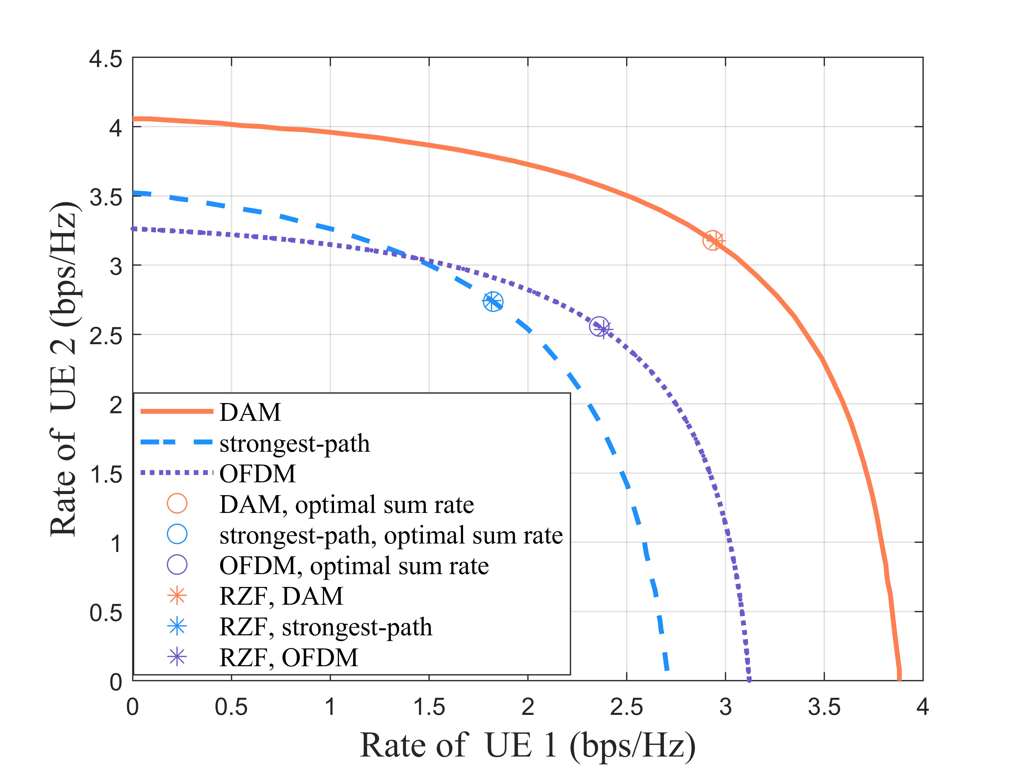
Figure 3: Achievable rate region of DAM, strongest-path beamforming, and OFDM.

Fig. 3 shows the Pareto boundary for multi-user DAM, the strongest-path-based beamforming and OFDM after considering the CP or the guard interval overhead. It is observed that the rate region of multi-user DAM is significantly larger than that of the two benchmarking schemes, thanks to its full utilization of all multi-path components and the low guard interval overhead. Besides, the performance of the RZF beamforming scheme approaches to the optimal sum rate on the pareto boundary, which demonstrates the superiority of the RZF beamforming.

Fig. 4 shows the spectral efficiency versus the transmit power for the proposed multi-user DAM transmission, the strongest-path-based beamforming and OFDM transmission, with MRT, ZF and RZF beamforming, respectively. It is observed that the proposed multi-user DAM transmission significantly outperforms the two benchmarking schemes for all the three beamforming strategies. This is expected since DAM makes full use of the multi-path signal components, as can be seen from the first term in (4), whereas the strongest-path-based beamforming only uses the strongest multi-path channel component as the desired signal. On the other hand, DAM is superior to OFDM since DAM requires less guard interval overhead than OFDM, as can be seen in (78) and (79). It is also observed that the low-complexity per-path based MRT beamforming achieves comparable performance as ZF and RZF schemes, especially in the low-power regime, thanks to the superior spatial resolution and multi-path sparsity of mmWave massive MIMO systems.

Fig. 5 studies the impact of the number of multi-paths on the spectral efficiency for the three schemes. It is observed that the proposed multi-user DAM transmission yields a better spectral efficiency performance than the benchmarking schemes, and both DAM transmission and OFDM show robustness to the increase of the multi-paths. By contrast, the performance of the strongest-path-based beamforming degrades significantly with the number of multi-paths. This is because DAM benefits from all the multi-paths components and OFDM transmits signals with parallel sub-carriers, while the strongest-path-based beamforming only uses the strongest multi-path channel component.

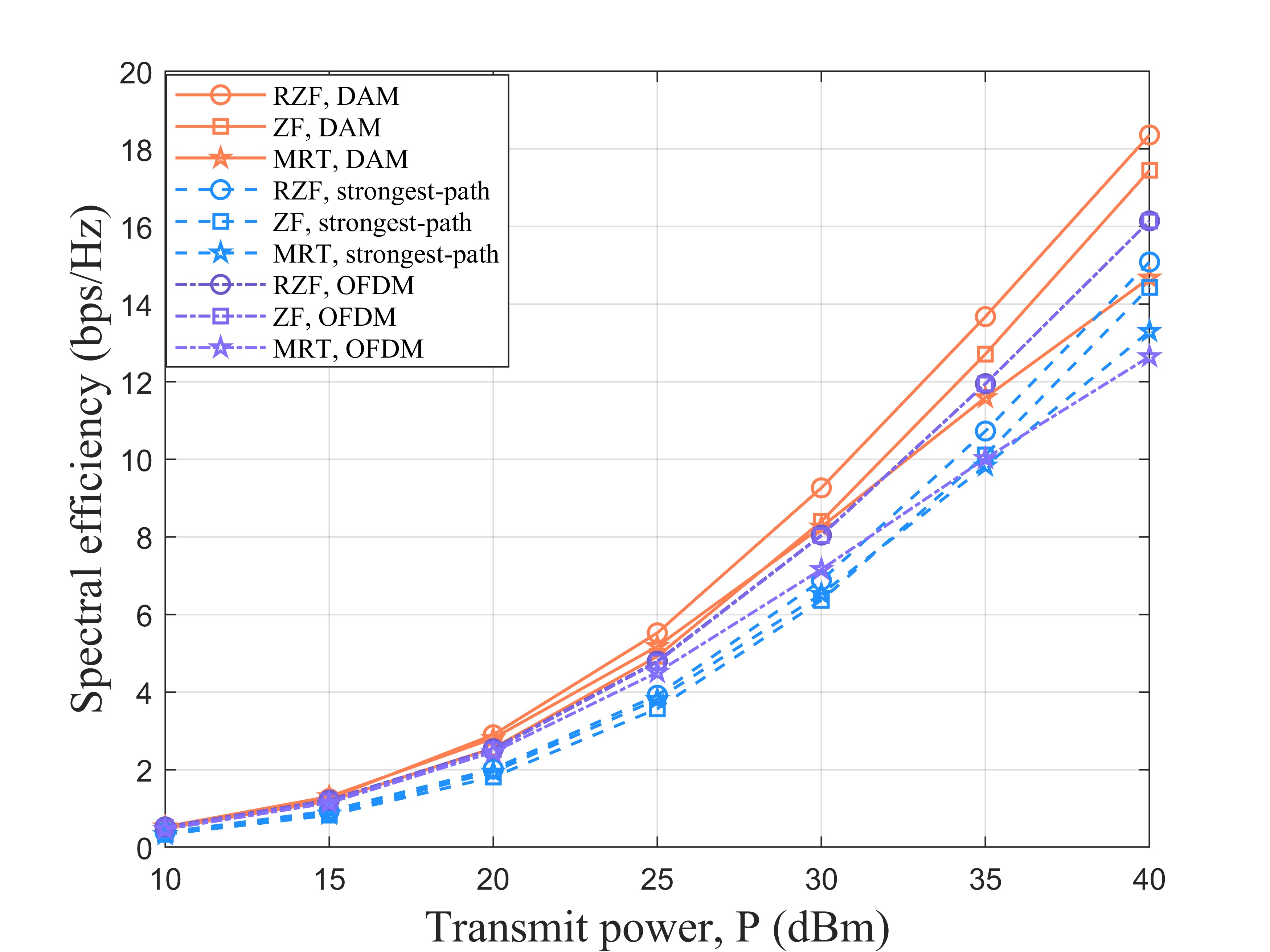
Figure 4: Spectral efficiency versus transmit power for the proposed multi-user DAM transmission, the strongest-path-based beamforming, and OFDM.

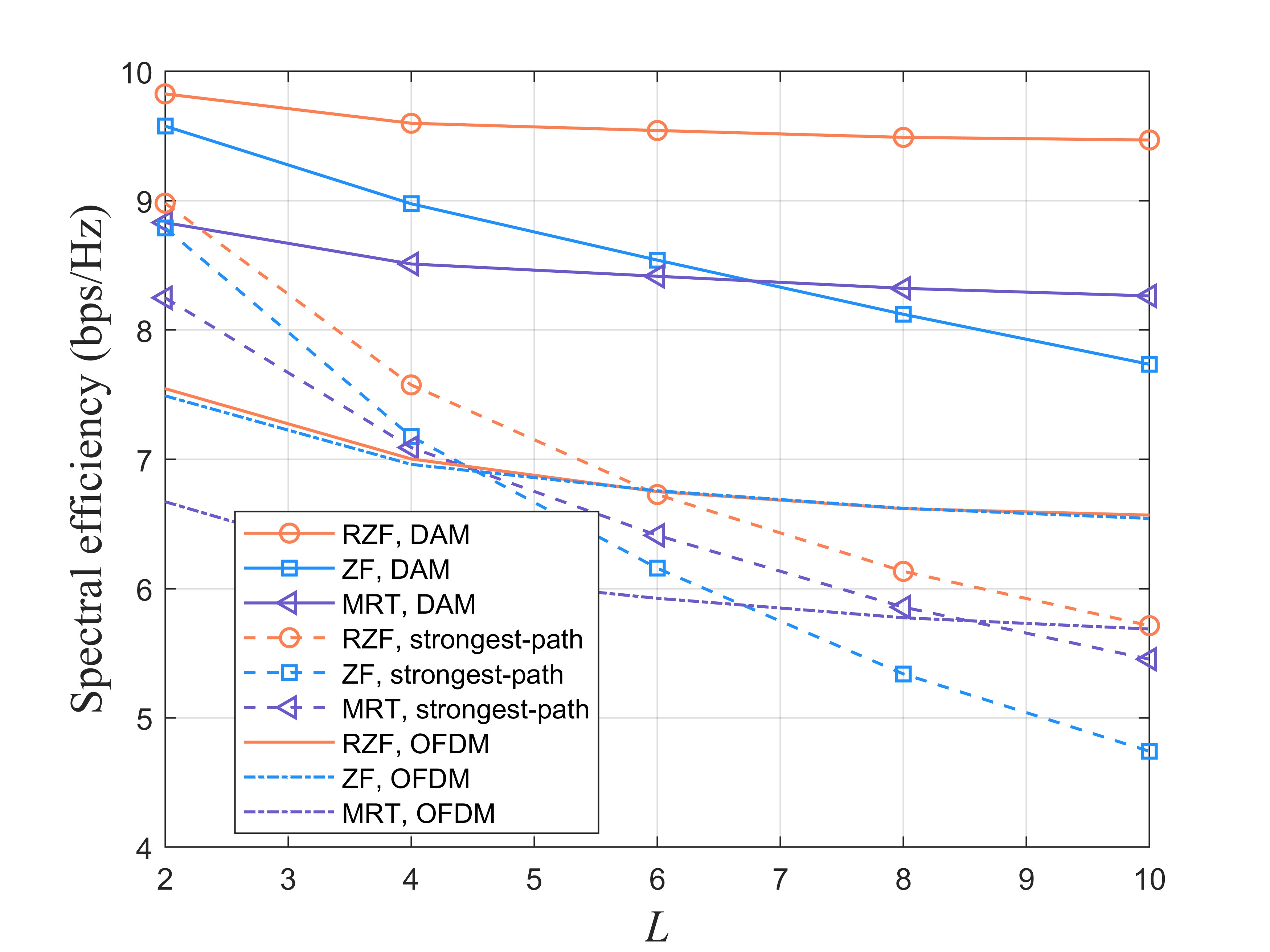
Figure 5: Spectral efficiency versus the number of multi-paths for the proposed multi-user DAM and the benchmarking strongest path scheme and OFDM transmission.

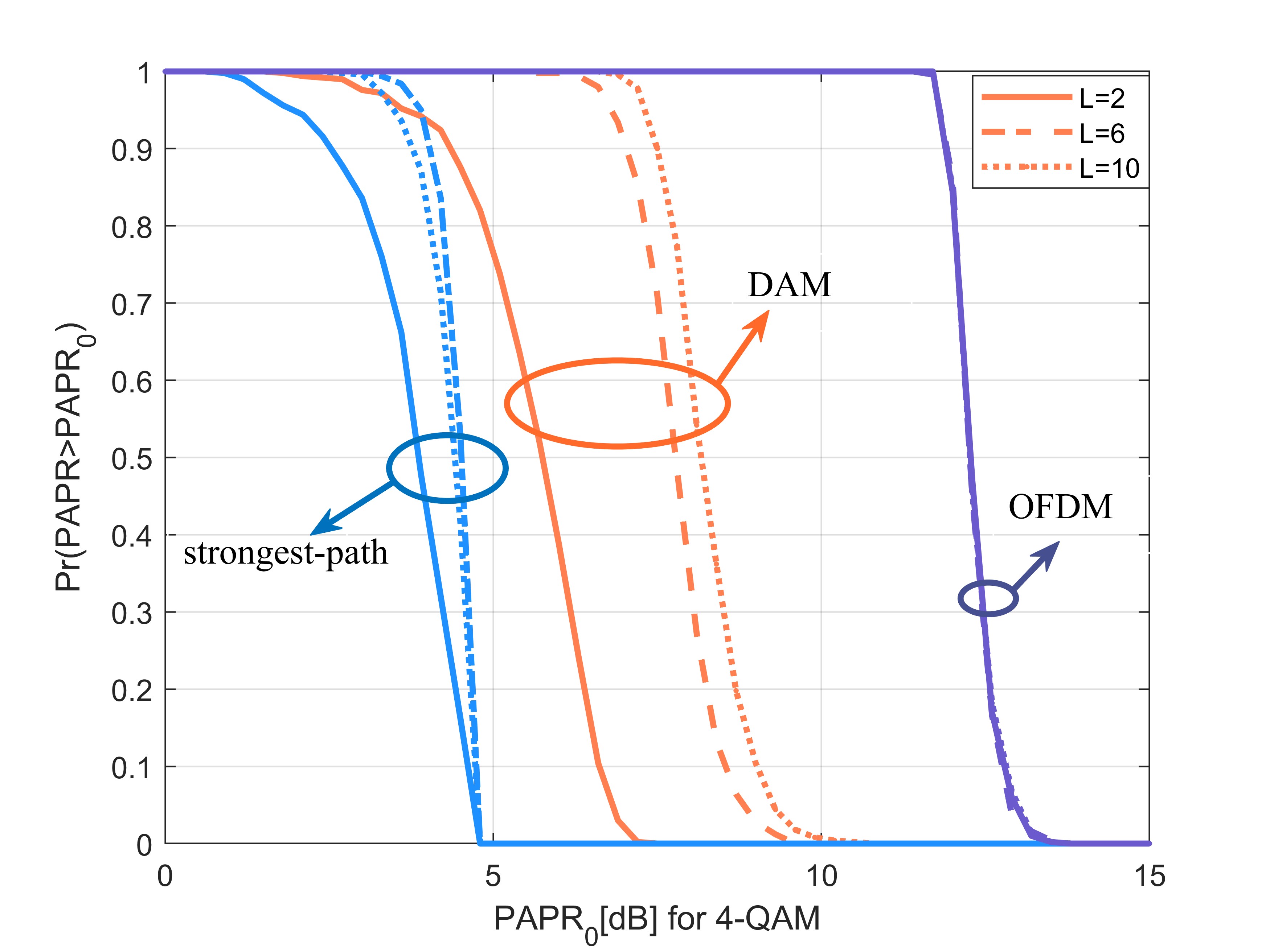
Figure 6: PAPR comparison for DAM transmission, OFDM, and the strongest-path-based scheme with 4-QAM modulation.

Last, Fig. 6 shows the PAPR comparison for the proposed multi-user DAM transmission, the strongest-path-based beamforming and OFDM with the corresponding MRT beamforming strategies, by adopting with 4-QAM. Specifically, the metric of complementary cumulative distribution function (CCDF) is considered to evaluate the PAPR performance. It is observed that the single-carrier DAM technique achieves significantly lower PAPR than OFDM. This is expected since for OFDM, a total of $KM$ singals are superimposed on each antenna, whereas for DAM, only $L_{\mathrm{tot}}$ multi-path signals are mixed on each antenna, as can be inferred from (86) and (82), respectively. On the other hand, the PAPR of DAM is slightly higher than the strongest-path-based beamforming, since the strongest-path-based beamforming only uses the single strongest path component as the desired signal, and thus $K$ signals are mixed on each antenna.

VII Conclusion

This paper investigated the performance of the multi-user DAM technique for mmWave massive MIMO communications. For the asymptotic case when the number of BS antennas is much larger than the total number of channel multi-paths, it was shown that both the ISI and IUI are completely eliminated with the simple per-path-based MRT beamforming and delay pre-compensation. For the general scenario with a finite number of BS antennas, the optimal achievable rate region for multi-user DAM system and benchmarking schemes were characterized. Next, three classical beamforming schemes were tailored for multi-user DAM communication in a per-path basis and benchmarking schemes, so as to maximize the sum rate, namely the per-path-based MRT, ZF and RZF beamforming. Moreover, the guard interval overhead and PAPR were analyzed for multi-user DAM and the two benchmarking schemes. Simulation results demonstrated that the proposed multi-user DAM transmission outperforms the benchmarking schemes of the strongest-path-based beamforming and OFDM in terms of spectral efficiency, and has a lower PAPR than OFDM.

References

- [1] X. Wang, H. Lu, and Y. Zeng, “Multi-user delay alignment modulation for millimeter wave massive MIMO,” in Proc. IEEE Global Commun. Conf. (GLOBECOM), 2023.
- [2] H. Lu and Y. Zeng, “Delay alignment modulation: Enabling equalization-free single-carrier communication,” IEEE Wireless Commun. Lett., vol. 11, no. 9, pp. 1785–1789, Sep. 2022.
- [3] E. Björnson, L. Sanguinetti, H. Wymeersch, J. Hoydis, and T. L. Marzetta, “Massive MIMO is a reality—what is next?: Five promising research directions for antenna arrays,” Digit. Signal Process., vol. 94, pp. 3–20, Nov. 2019.
- [4] H. Lu and Y. Zeng, “Communicating with extremely large-scale array/surface: Unified modeling and performance analysis,” IEEE Trans. Wireless Commun., vol. 21, no. 6, pp. 4039–4053, Jun. 2022.
- [5] M. R. Akdeniz, Y. Liu, M. K. Samimi, S. Sun, S. Rangan, T. S. Rappaport, and E. Erkip, “Millimeter wave channel modeling and cellular capacity evaluation,” IEEE J. Sel. Areas Commun., vol. 32, no. 6, pp. 1164–1179, Jun. 2014.
- [6] D. Ding and Y. Zeng, “Channel estimation for delay alignment modulation,” arXiv preprints arXiv:2206.09339, Jun. 2022.
- [7] H. Lu and Y. Zeng, “Delay alignment modulation: manipulating channel delay spread for efficient single- and multi-carrier communication,” IEEE Trans. Commun., 2023, doi: 10.1109/TCOMM.2023.3306898.
- [8] Z. Xiao and Y. Zeng, “Integrated sensing and communication with delay alignment modulation: Performance analysis and beamforming optimization,” IEEE Trans. Wireless Commun., Apr. 2023.
- [9] Z. Wang, X. Mu, and Y. Liu, “Bidirectional integrated sensing and communication: Full-duplex or half-duplex?” arXiv preprints arXiv:2210.14112, Oct. 2022.
- [10] H. Lu, Y. Zeng, S. Jin, and R. Zhang, “Single-carrier delay alignment modulation for multi-IRS aided communication,” IEEE Trans. Wireless Commun., 2023, doi: 10.1109/TWC.2023.3306899.
- [11] F. Han, Y.-H. Yang, B. Wang, Y. Wu, and K. J. R. Liu, “Time-reversal division multiple access over multi-path channels,” IEEE Trans. Commun., vol. 60, no. 7, pp. 1953–1965, Jul. 2012.
- [12] A. Pitarokoilis, S. K. Mohammed, and E. G. Larsson, “On the optimality of single-carrier transmission in large-scale antenna systems,” IEEE Wireless Commun. Lett., vol. 1, no. 4, pp. 276–279, Aug. 2012.
- [13] P. Melsa, R. Younce, and C. Rohrs, “Impulse response shortening for discrete multitone transceivers,” IEEE Trans. Commun., vol. 44, no. 12, pp. 1662–1672, Dec. 1996.
- [14] R. Martin, K. Vanbleu, M. Ding, G. Ysebaert, M. Milosevic, B. Evans, M. Moonen, and C. Johnson, “Unification and evaluation of equalization structures and design algorithms for discrete multitone modulation systems,” IEEE Trans. Signal Process., vol. 53, no. 10, pp. 3880–3894, Oct. 2005.
- [15] S. Li, W. Yuan, J. Yuan, B. Bai, D. Wing Kwan Ng, and L. Hanzo, “Time-domain vs. frequency-domain equalization for FTN signaling,” IEEE Trans. Veh. Technol., vol. 69, no. 8, pp. 9174–9179, Aug. 2020.
- [16] A. Goldsmith, Wireless Communications. Cambridge University Press, 2005.
- [17] Y. Hong, T. Thaj, and E. Viterbo, Delay-Doppler Communications: Principles and Applications. Amsterdam: Academic Press, 2022.
- [18] L. Xiao, S. Li, Y. Qian, D. Chen, and T. Jiang, “An overview of OTFS for internet of things: Concepts, benefits, and challenges,” IEEE Internet Things J., vol. 9, no. 10, pp. 7596–7618, May 2022.
- [19] T. Taniguchi, H. H. Pham, N. X. Tran, and Y. Karasawa, “Maximum SINR design method of MIMO communication systems using tapped delay line structure in receiver side,” in Proc. IEEE Veh. Technol. Conf., vol. 2, May 2004, pp. 799–803.
- [20] Y.-C. Liang and J. Cioffi, “Combining transmit beamforming, space-time block coding and delay spread reduction,” in Proc. Personal, Indoor and Mobile Radio Commun. (PIMRC), vol. 1, Sep. 2003, pp. 105–109.
- [21] Y. Zeng and R. Zhang, “Millimeter wave MIMO with lens antenna array: A new path division multiplexing paradigm,” IEEE Trans. Commun., vol. 64, no. 4, pp. 1557–1571, Apr. 2016.
- [22] G. Wang, J. Sun, and G. Ascheid, “Hybrid beamforming with time delay compensation for millimeter wave MIMO frequency selective channels,” in Proc. IEEE Veh. Technol. Conf., May 2016, pp. 1–6.
- [23] X. Song, S. Haghighatshoar, and G. Caire, “Efficient beam alignment for millimeter wave single-carrier systems with hybrid MIMO transceivers,” IEEE Trans. Wireless Commun., vol. 18, no. 3, pp. 1518–1533, Mar. 2019.
- [24] L. Miretti, T. Kühne, A. Schultze, W. Keusgen, G. Caire, M. Peter, S. Stańczak, and T. Eichler, “Little or no equalization is needed in energy-efficient sub-THz mobile access,” arXiv preprints arXiv:2210.05806, Oct. 2022.
- [25] R. Zhang and S. Cui, “Cooperative interference management with MISO beamforming,” IEEE Trans. Signal Process., vol. 58, no. 10, pp. 5450–5458, Jul. 2010.
- [26] Y. Zeng, R. Zhang, E. Gunawan, and Y. L. Guan, “Optimized transmission with improper gaussian signaling in the K-user MISO interference channel,” IEEE Trans. Wireless Commun., vol. 12, no. 12, pp. 6303–6313, Dec. 2013.
- [27] M. Bengtsson and B. Ottersten, “Optimal and suboptimal transmit beamforming,” Handbook of Antennas in Wireless Communications, 2001.
- [28] M. Grant and S. Boyd, “CVX: Matlab software for disciplined convex programming,” [Online]. Available: ttp://stanford.edu/boyd/cvx.
- [29] Y. Zeng, Q. Wu, and R. Zhang, “Accessing from the sky: A tutorial on UAV communications for 5G and beyond,” Proc. IEEE, vol. 107, no. 12, pp. 2327–2375, Dec. 2019.
- [30] C. Peel, B. Hochwald, and A. Swindlehurst, “A vector-perturbation technique for near-capacity multiantenna multiuser communication-part I: channel inversion and regularization,” IEEE Trans. Commun., vol. 53, no. 1, pp. 195–202, Oct. 2005.
- [31] C. Ni, Y. Ma, and T. Jiang, “A novel adaptive tone reservation scheme for PAPR reduction in large-scale multi-user MIMO-OFDM systems,” IEEE Wireless Commun. Lett., vol. 5, no. 5, pp. 480–483, Oct. 2016.