Learning multi-modal generative models with permutation-invariant encoders and tighter variational bounds

Abstract

Devising deep latent variable models for multi-modal data has been a long-standing theme in machine learning research. Multi-modal Variational Autoencoders (VAEs) have been a popular generative model class that learns latent representations which jointly explain multiple modalities. Various objective functions for such models have been suggested, often motivated as lower bounds on the multi-modal data log-likelihood or from information-theoretic considerations. In order to encode latent variables from different modality subsets, Product-of-Experts (PoE) or Mixture-of-Experts (MoE) aggregation schemes have been routinely used and shown to yield different trade-offs, for instance, regarding their generative quality or consistency across multiple modalities. In this work, we consider a variational bound that can tightly lower bound the data log-likelihood. We develop more flexible aggregation schemes that generalise PoE or MoE approaches by combining encoded features from different modalities based on permutation-invariant neural networks. Our numerical experiments illustrate trade-offs for multi-modal variational bounds and various aggregation schemes. We show that tighter variational bounds and more flexible aggregation models can become beneficial when one wants to approximate the true joint distribution over observed modalities and latent variables in identifiable models.

1 Introduction

Multi-modal data sets where each sample has features from distinct sources have grown in recent years. For example, multi-omics data such as genomics, epigenomics, transcriptomics and metabolomics can provide a more comprehensive understanding of biological systems if multiple modalities are analysed in an integrative framework [7, 74, 90]. However, annotations or labels in such data sets are often rare, making unsupervised or semi-supervised generative approaches particularly attractive as such methods can be used in these settings to (i) generate data, such as missing modalities, and (ii) learn latent representations that are useful for down-stream analyses or that are of scientific interest themselves.

The availability of heterogenous data for different modalities promises to learn generalizable representations that can capture shared content across multiple modalities in addition to modality-specific information. A promising class of weakly-supervised generative models is multi-modal VAEs [117, 138, 110, 115] that combine information across modalities in an often-shared low-dimensional latent representation. Other classes of generative models, such as denoising diffusion or energy-based models, have achieved impressive generative quality. However, these models are not naturally learning multi-modal latent representations and commonly resort to different guidance techniques [24, 47] to generate samples that are coherent across multiple modalities.

Non-linear latent variable models often lack identifiability, even up to indeterminacies, which makes it hard to interpret inferred latent representations or model parameters. However, utilizing auxiliary variables or additional modalities, recent work [62, 63, 139] has shown that such models can become identifiable up to known indeterminacies with such models adapted, for instance, to neuroscience applications: [151] model neural activity conditional on non-neural labels using VAEs, while [107] model neural recordings conditional on behavioural variables using self-supervised learning. A common route for learning the parameters of latent variable models is via maximization of the marginal data likelihood with various lower bounds thereof suggested in previous work.

Setup.

We consider a set of $M$ random variables $\{X_{1},\ldots,X_{M}\}$ with empirical density $p_{d}$, where each random variable $X_{s}$, $s\in\mathcal{M}=\{1,\dots,M\}$, can be used to model a different data modality taking values in $\mathsf{X}_{s}$. With some abuse of notation, we write $X=\{X_{1},\ldots,X_{M}\}$ and for any subset $\mathcal{S}\subset\mathcal{M}$, we set $X=(X_{\mathcal{S}},X_{\setminus\mathcal{S}})$ for two partitions of the random variables into $X_{\mathcal{S}}=\{X_{s}\}_{s\in\mathcal{S}}$ and $X_{\setminus\mathcal{S}}=\{X_{s}\}_{s\in\mathcal{M}\setminus\mathcal{S}}$. We pursue a latent variable model setup, analogous to uni-modal VAEs [66, 100]. For a latent variable $Z\in\mathsf{Z}$ with prior density $p_{\theta}(z)$, we posit a joint generative model $p_{\theta}(z,x)=p_{\theta}(z)\prod_{s=1}^{M}p_{\theta}(x_{s}|z)$, where $p_{\theta}(x_{s}|z)$ is commonly referred to as the decoding distribution for modality $s$. Observe that all modalities are independent given the latent variable $z$ shared across all modalities. One can introduce modality-specific latent variables by making sparsity assumptions for the decoding distribution. We assume throughout that $\mathsf{Z}=\mathbb{R}^{D}$, and that $p_{\theta}(z)$ is a Lebesgue density, although the results can be extended to more general settings such as discrete random variables $Z$ with appropriate adjustments, for instance, regarding the gradient estimators.

Multi-modal variational bounds and mutual information.

Popular approaches to train multi-modal models are based on a mixture-based variational bound [22, 110] given by $\mathcal{L}^{\text{Mix}}(\theta,\phi,\beta)=\int\rho(S)\mathcal{L}^{\text{Mix}}_{\mathcal{S}}(x,\theta,\phi,\beta)\mathrm{d}\mathcal{S}$, where

$$\mathcal{L}^{\text{Mix}}_{\mathcal{S}}(x,\theta,\phi,\beta)=\int q_{\phi}(z|x_{\mathcal{S}})\left[\log p_{\theta}(x|z)\right]\mathrm{d}z-\beta\mathsf{K}\mathsf{L}(q_{\phi}(z|x_{\mathcal{S}})|p_{\theta}(z))$$ (1)

and $\rho$ is some distribution on the power set $\mathcal{P}(\mathcal{M})$ of $\mathcal{M}$ and $\beta>0$. For $\beta=1$, one obtains the bound $\mathcal{L}^{\text{Mix}}_{\mathcal{S}}(x,\theta,\phi,\beta)\leq\log p_{\theta}(x)$. Variations of (1) have been suggested [114], for example, by replacing the prior density $p_{\theta}$ in the KL-term by a weighted product of the prior density $p_{\theta}$ and the uni-modal encoding distributions $q_{\phi}(z|x_{s})$, for all $s\in\mathcal{M}$. Maximizing $\mathcal{L}^{\text{Mix}}_{\mathcal{S}}$ can be seen as

$$\text{minimizing }\left\{\mathcal{H}(X|Z_{\mathcal{S}})+\beta\operatorname{I}_{q_{\phi}}(X_{\mathcal{S}},Z_{\mathcal{S}})=\mathcal{H}(X)-\operatorname{I}_{q_{\phi}}(X,Z_{\mathcal{S}})+\beta\operatorname{I}_{q_{\phi}}(X_{\mathcal{S}},Z_{\mathcal{S}})\right\},$$ (2)

where $I_{q}(X,Y)=\int q(x,y)\log\frac{q(x,y)}{q(x)q(y)}$ is the mutual information of random variables $X$ and $Y$ having marginal and joint densities $q$, whilst $\mathcal{H}(X|Y)=-\int q(x,y)\log q(x|y)]\mathrm{d}x\mathrm{d}y$ is the conditional entropy of $X$ given $Y$. Likewise, the multi-view variational information bottleneck approach developed in [74] for predicting $x_{\setminus\mathcal{S}}$ given $x_{\mathcal{S}}$ can be interpreted as minimizing $-\operatorname{I}_{q_{\phi}}(X_{\setminus\mathcal{S}},Z)+\beta\operatorname{I}_{q_{\phi}}(X_{\mathcal{S}},Z)$. [52] suggested a related bound motivated by a conditional variational bottleneck perspective that aims to maximize the reduction of total correlation of $X$ when conditioned on $Z$, as measured by the conditional total correlation, see [136, 127, 32], i.e.,

$$\text{minimizing }\Big{\{}\text{TC}(X|Z)=\text{TC}(X)-\text{TC}(X,Z)=\text{TC}(X)+\operatorname{I}_{q_{\phi}}(X,Z)-\sum_{s=1}^{M}\operatorname{I}_{q_{\phi}}(X_{s},Z)\Big{\}},$$ (3)

where $\text{TC}(X)=\mathsf{K}\mathsf{L}(p(x)|\prod_{i=1}^{d}p(x_{i}))$ for $d$-dimensional $X$. Resorting to variational lower bounds and using a constant $\beta>0$ that weights the contributions of the mutual information terms, approximations of (3) can be optimized by maximizing

$$\mathcal{L}^{\text{TC}}(\theta,\phi,\beta)=\int\rho(\mathcal{S})\int\left\{q_{\phi}(z|x)\left[\log p_{\theta}(x|z)\right]\mathrm{d}z-\beta\mathsf{K}\mathsf{L}(q_{\phi}(z|x)|q_{\phi}(z|x_{\mathcal{S}}))\right\}\mathrm{d}\mathcal{S},$$

where $\rho$ is concentrated on the uni-modal subsets of $\mathcal{M}$. Similar bounds have been suggested in [114] and [117] by considering different KL-regularisation terms, see also [116]. [111] add a contrastive term to the maximum likelihood objective and minimize $-\log p_{\theta}(x)-\beta\operatorname{I}_{p_{\theta}}(X_{\mathcal{S}},X_{\setminus\mathcal{S}})$.

Multi-modal aggregation schemes.

In order to optimize the variational bounds above or to allow for flexible conditioning at test time, we need to learn encoding distributions $q_{\phi}(z|x_{\mathcal{S}})$ for any $\mathcal{S}\in\mathcal{P}({\mathcal{M}})$. The typical aggregation schemes that are scalable to a large number of modalities are based on a choice of uni-modal encoding distributions $q_{\phi_{s}}(z|x_{s})$ for any $s\in\mathcal{M}$, which are then used to define the multi-modal encoding distributions as follows:

• Mixture of Experts (MoE), see [110], $q_{\phi}^{\text{MoE}}(z|x_{\mathcal{S}})=\frac{1}{|\mathcal{S}|}\sum_{s\in\mathcal{S}}q_{\phi_{s}}(z|x_{s})$.

• Product of Experts (PoE), see [137], $q_{\phi}^{\text{PoE}}(z|x_{\mathcal{S}})=\frac{1}{\mathcal{Z}}p_{\theta}(z)\prod_{s\in\mathcal{S}}q_{\phi_{s}}(z|x_{s})$, for some $\mathcal{Z}\in\mathbb{R}$.

Contributions.

This paper contributes (i) a new variational bound that addresses known limitations of previous variational bounds. For instance, mixture-based bounds (1) may not provide tight bounds on the joint log-likelihood if there is considerable modality-specific variation [22]. In contrast, the novel variational bound becomes a tight lower bound of both the marginal log-likelihood $\log p_{\theta}(x_{\mathcal{S}})$ as well as the conditional $\log p_{\theta}(x_{\setminus\mathcal{S}}|x_{\mathcal{S}})$ for any choice of $\mathcal{S}\in\mathcal{P}(\mathcal{M})$, provided that we can learn a flexible multi-modal encoding distribution. This paper then contributes (ii) new multi-modal aggregation schemes that yield more expressive multi-modal encoding distributions when compared to MoEs or PoEs. These schemes are motivated by the flexibility of permutation-invariant architectures such as DeepSets [144] or attention models [125, 75]. We illustrate that these innovations (iii) are beneficial when learning identifiable models, aided by using flexible prior and encoding distributions consisting of mixtures and (iv) yield higher log-likelihoods in experiments.

Further related work.

Canonical Correlation Analysis [49] is a classical approach for multi-modal data that aims to find projections of two modalities by maximally correlating them and has been interpreted in a probabilistic or generative framework [9]. Furthermore, it has been extended to include more than two modalities [6, 119] or to allow for non-linear transformations [2, 42, 132, 61]. Probabilistic CCA can also be seen as multi-battery factor analysis (MBFA) [17, 69], wherein a shared latent variable models the variation common to all modalities with modality-specific latent variables capturing the remaining variation. Likewise, latent factor regression or classification models [113] assume that observed features and response are driven jointly by a latent variable. [126] considered a tiple-ELBO for two modalities, while [115] introduced a generalised variational bound that involves a summation over all modality subsets. A series of work has developed multi-modal VAEs based on shared and private latent variables [133, 76, 84, 85, 97]. [123] proposed a hybrid generative-discriminative objective and minimized an approximation of the Wasserstein distance between the generated and observed multi-modal data. [60] consider a semi-supervised setup of two modalities that requires no explicit multi-modal aggregation function. Extending the Info-Max principle [81], maximizing mutual information $\operatorname{I}_{q}(g_{1}(X_{1}),g(X_{2}))\leq\operatorname{I}_{q}((X_{1},X_{2}),(Z_{1},Z_{2}))$ based on representations $Z_{s}=g_{s}(X_{s})$ for modality-specific encoders $g_{s}$ from two modalities has been a motivation for approaches based on (symmetrised) contrastive objectives [120, 148, 23] such as InfoNCE [96, 98, 131] as a variational lower bound on the mutual information between $Z_{1}$ and $Z_{2}$.

2 A tighter variational bound with arbitrary modality masking

For $\mathcal{S}\subset\mathcal{M}$ and $\beta>0$, we define

$$\mathcal{L}_{\mathcal{S}}(x_{\mathcal{S}},\theta,\phi,\beta)=\int q_{\phi}(z|x_{\mathcal{S}})\left[\log p_{\theta}(x_{\mathcal{S}}|z)\right]\mathrm{d}z-\beta\mathsf{K}\mathsf{L}(q_{\phi}(z|x_{\mathcal{S}})|p_{\theta}(z)).$$ (4)

This is simply a standard variational lower bound [59, 14] restricted to the subset $\mathcal{S}$ for $\beta=1$, and therefore $\mathcal{L}_{\mathcal{S}}(x_{\mathcal{S}},\theta,\phi,1)\leq\log p_{\theta}(x_{\mathcal{S}})$. To obtain a lower bound on the log-likelihood of all modalities, we introduce an (approximate) conditional lower bound

$$\mathcal{L}_{\setminus\mathcal{S}}(x,\theta,\phi,\beta)=\int q_{\phi}(z|x)\left[\log p_{\theta}(x_{\setminus\mathcal{S}}|z)\right]\mathrm{d}z-\beta\mathsf{K}\mathsf{L}(q_{\phi}(z|x)|q_{\phi}(z|x_{\mathcal{S}})).$$ (5)

For some fixed density $\rho$ on $\mathcal{P}(\mathcal{M})$, we suggest the overall bound

$$\mathcal{L}(x,\theta,\phi,\beta)=\int\rho(\mathcal{S})\left[\mathcal{L}_{\mathcal{S}}(x_{\mathcal{S}},\theta,\phi,\beta)+\mathcal{L}_{\setminus\mathcal{S}}(x,\theta,\phi,\beta)\right]\mathrm{d}\mathcal{S},$$

which is a generalisation of the bound suggested in [138] to an arbitrary number of modalities. This bound can be optimised using standard Monte Carlo techniques, for example, by computing unbiased pathwise gradients [66, 100, 122] using the reparameterisation trick. For variational families such as Gaussian mixtures, one can employ implicit reparameterisation [29]. It is straightforward to adapt variance reduction techniques such as ignoring the score term of the multi-modal encoding densities for pathwise gradients [101], see Algorithm 1 in Appendix K for pseudo-code. Nevertheless, a scalable approach requires an encoding technique that allows to condition on any masked modalities with a computational complexity that does not increase exponentially in $M$.

Remark (Optimization, multi-task learning and the choice of $\rho$).

For simplicity, we have chosen to sample $\mathcal{S}\sim\rho$ in our experiments via the hierarchical construction $\gamma\sim\mathcal{U}(0,1)$, $m_{j}\sim\text{Bern}(\gamma)$ iid for all $j\in[M]$ and setting $\mathcal{S}=\{s\in[M]\colon m_{j}=1\}$. The distribution $\rho$ for masking the modalities can be adjusted to accommodate various weights for different modality subsets. Indeed, (2) can be seen as a linear scalarisation of a multi-task learning problem [30, 109]. We aim to optimise a loss vector $(\mathcal{L}_{\mathcal{S}}+\mathcal{L}_{\setminus\mathcal{S}})_{\mathcal{S}\subset\mathcal{M}}$, where the gradients for each $\mathcal{S}\subset\mathcal{M}$ can point in different directions, making it challenging to minimise the loss for all modalities simultaneously. Consequently, [56] used multi-task learning techniques (e.g., as suggested in [19, 142]) for adjusting the gradients in mixture based VAEs. Such improved optimisation routines are orthogonal to our approach. Similarly, we do not analyse optimisation issues such as initialisations and training dynamics that have been found challenging for multi-modal learning [134, 51].

Multi-modal distribution matching.

Likelihood-based learning approaches aim to match the model distribution $p_{\theta}(x)$ to the true data distribution $p_{d}(x)$. Variational approaches achieve this by matching in the latent space the encoding distribution to the true posterior as well as maximizing a tight lower bound on $\log p_{\theta}(x)$, see for instance [103]. We show here analogous results for the multi-modal variational bound. Consider therefore the densities $p_{\theta}(z,x)=p_{\theta}(z)p_{\theta}(x_{\mathcal{S}}|z)p_{\theta}(x_{\setminus\mathcal{S}}|z)$ and $q_{\phi}(z,x)=p_{d}(x)q_{\phi}(z|x)=p_{d}(x_{\mathcal{S}})q_{\phi}(z|x_{\mathcal{S}})q_{\phi}(x_{\setminus\mathcal{S}}|z,x_{\mathcal{S}})$. The standard interpretation is that the former is the generative density, while the latter is the encoding path consisting of the conditional variational approximation $q_{\phi}$ and the empirical density $p_{d}$. The following Proposition, proven in Appendix A, shows that maximizing the variational lower bound $\mathcal{L}$ leads to a joint distribution matching of $q_{\phi}(z,x)$ and $p_{\theta}(z,x)$, analogously to the uni-modal setting [150].

Proposition (Joint distribution matching).

For any $\mathcal{S}\in\mathcal{P}(\mathcal{M})$, we have that

$$\int p_{d}(x)\left[\mathcal{L}_{\mathcal{S}}(x_{\mathcal{S}},\theta,\phi,1)+\mathcal{L}_{\setminus\mathcal{S}}(x,\theta,\phi,1)\right]\mathrm{d}x+\mathcal{H}(p_{d}(x))=-\mathsf{K}\mathsf{L}(q_{\phi}(z,x)|p_{\theta}(z,x)).$$

In particular, $\mathcal{L}_{\mathcal{S}}(x_{\mathcal{S}},\theta,\phi,1)+\mathcal{L}_{\setminus\mathcal{S}}(x,\theta,\phi,1)$ is a lower bound on $\log p_{\theta}(x)$.

Moreover, Proposition A in Appendix A illustrates that maximizing $\int p_{d}(x_{\mathcal{S}})\mathcal{L}_{\mathcal{S}}(x_{\mathcal{S}},\theta,\phi)\mathrm{d}x_{\mathcal{S}}$ drives (i) the joint inference distribution $q_{\phi}(z,x_{\mathcal{S}})=p_{d}(x_{\mathcal{S}})q_{\phi}(z|x_{\mathcal{S}})$ of the $\mathcal{S}$ submodalities to the joint generative distribution $p_{\theta}(z,x_{\mathcal{S}})=p_{\theta}(z)p_{\theta}(x_{\mathcal{S}}|z)$ and (ii) the generative marginal $p_{\theta}(x_{\mathcal{S}})$ to its empirical counterpart $p_{d}(x_{\mathcal{S}})$. Analogously, maximizing $\int p_{d}(x_{\setminus\mathcal{S}}|x_{\mathcal{S}})\mathcal{L}_{\setminus\mathcal{S}}(x,\theta,\phi)\mathrm{d}x_{\setminus\mathcal{S}}$ drives (i) the distribution $p_{d}(x_{\setminus\mathcal{S}}|x_{\mathcal{S}})q_{\phi}(z|x)$ to the distribution $p_{\theta}(x_{\setminus\mathcal{S}}|z)q_{\phi}(z|x_{\mathcal{S}})$ and (ii) the conditional $p_{\theta}(x_{\setminus\mathcal{S}}|x_{\mathcal{S}})$ to its empirical counterpart $p_{d}(x_{\setminus\mathcal{S}}|x_{\mathcal{S}})$, provided that $q_{\phi}(z|x_{\mathcal{S}})$ approximates $p_{\theta}(z|x_{\mathcal{S}})$ exactly. In this case, Proposition A implies that $\mathcal{L}_{\setminus\mathcal{S}}(x,\theta,\phi)$ is a lower bound of $\log p_{\theta}(x_{\setminus\mathcal{S}}|x_{\mathcal{S}})$. Furthermore, it shows that $\mathcal{L}_{\setminus\mathcal{S}}(x,\theta,\phi)$ contains a Bayes-consistency matching term for the multi-modal encoders where a mismatch can yield poor cross-generation, as an analogue of the prior not matching the aggregated posterior [87] leading to poor unconditional generation, see Remark A. Our problem setup recovers meta-learning with (latent) Neural processes [34] when only optimizing the variational term $\mathcal{L}_{\setminus\mathcal{S}}$, where $\mathcal{S}$ is determined by context-target splits, cf. Appendix B.

Information-theoretic perspective.

Beyond generative modelling, $\beta$-VAEs [46] have been popular for representation learning and data reconstruction. [3] suggest learning a latent representation that achieves certain mutual information with the data based on upper and lower variational bounds of the mutual information. A Legendre transformation thereof recovers the $\beta$-VAE objective and allows a trade-off between information content or rate versus reconstruction quality or distortion. We show that the proposed variational objective gives rise to an analogous perspective for multiple modalities. We recall first that mutual information $\operatorname{I}_{q_{\phi}}(X_{\mathcal{S}},Z)$ can be bounded by standard [11, 4, 3] lower and upper bounds using the rate and distortion:

$$\mathcal{H}_{\mathcal{S}}-D_{\mathcal{S}}\leq\mathcal{H}_{\mathcal{S}}-D_{\mathcal{S}}+\Delta_{1}=\operatorname{I}_{q_{\phi}}(X_{\mathcal{S}},Z)=R_{\mathcal{S}}-\Delta_{2}\leq R_{\mathcal{S}},$$ (6)

with $\Delta_{1},\Delta_{2}\geq 0$ for the rate $R_{\mathcal{S}}=\int p_{d}(x_{\mathcal{S}})\mathsf{K}\mathsf{L}(q_{\phi}(z|x_{\mathcal{S}})|p_{\theta}(z))\mathrm{d}x_{\mathcal{S}}$ measuring the information content that is encoded by $q_{\phi}$ into the latents, and the distortion $D_{\mathcal{S}}=-\int q_{\phi}(x_{\mathcal{S}},z)\log p_{\theta}(x_{\mathcal{S}}|z)\mathrm{d}z\mathrm{d}x_{\mathcal{S}}$ given as the negative reconstruction log-likelihood. Observe that $-\int p_{d}(x_{\mathcal{S}})\mathcal{L}(x_{\mathcal{S}})\mathrm{d}x_{\mathcal{S}}=D_{\mathcal{S}}+\beta R_{\mathcal{S}}$ and for any $\beta>0$, it holds that $\mathcal{H}_{\mathcal{S}}\leq R_{\mathcal{S}}+D_{\mathcal{S}}$. To arrive at a similar interpretation for the conditional bound $\mathcal{L}_{\setminus\mathcal{S}}$, we set $R_{\setminus\mathcal{S}}=\int p_{d}(x)\mathsf{K}\mathsf{L}(q_{\phi}(z|x)|q_{\phi}(z|x_{\mathcal{S}}))\mathrm{d}x$ for a conditional or cross rate. Similarly, set $D_{\setminus\mathcal{S}}=-\int p_{d}(x)q_{\phi}(z|x)\log p_{\theta}(x_{\setminus\mathcal{S}}|z)\mathrm{d}z\mathrm{d}x$. One obtains the following bounds, see Appendix A.

Lemma (Variational bounds on the conditional mutual information).

It holds that $-\int\mathcal{L}_{\setminus\mathcal{S}}(x,\theta,\phi,\beta)p_{d}(\mathrm{d}x)=D_{\setminus\mathcal{S}}+\beta R_{\setminus\mathcal{S}}$ and for $\Delta_{\setminus\mathcal{S},1},\Delta_{\setminus\mathcal{S},2}\geq 0$,

$$\mathcal{H}_{\setminus\mathcal{S}}-D_{\setminus\mathcal{S}}+\Delta_{\setminus\mathcal{S},1}=\operatorname{I}_{q_{\phi}}(X_{\setminus\mathcal{S}},Z_{\mathcal{M}}|X_{\mathcal{S}})=R_{\setminus\mathcal{S}}-\Delta_{\setminus\mathcal{S},2}.$$

Using the chain rules for entropy, we obtain that the suggested bound can be seen as a relaxation of bounds on marginal and conditional mutual information.

Corollary (Lagrangian relaxation).

It holds that

$$\mathcal{H}-D_{\mathcal{S}}-D_{\setminus\mathcal{S}}\leq\operatorname{I}_{q_{\phi}}(X_{\mathcal{S}},Z_{\mathcal{S}})+\operatorname{I}_{q_{\phi}}(X_{\setminus\mathcal{S}},Z_{\mathcal{M}}|X_{\mathcal{S}})\leq R_{\mathcal{S}}+R_{\setminus\mathcal{S}}$$

and minimizing $\mathcal{L}$ for fixed $\beta=\frac{\partial(D_{\mathcal{S}}+D_{\setminus\mathcal{S}})}{\partial(R_{\mathcal{S}}+R_{\setminus\mathcal{S}})}$ minimizes the rates $R_{\mathcal{S}}+R_{\setminus\mathcal{S}}$ and distortions $D_{\mathcal{S}}+D_{\setminus\mathcal{S}}$.

Remark (Mixture based variational bound).

Rephrasing the arguments in [22], we can write $-\int p_{d}(\mathrm{d}x)\mathcal{L}^{\text{Mix}}_{\mathcal{S}}(x)=D_{\mathcal{S}}+D^{c}_{\setminus\mathcal{S}}+\beta R_{\mathcal{S}}$, where $D^{c}_{\setminus\mathcal{S}}=\int p_{d}(x_{\mathcal{S}})q_{\phi}(z|x_{\mathcal{S}})\log p_{\theta}(x_{\setminus\mathcal{S}}|z)\mathrm{d}z\mathrm{d}x_{\mathcal{S}}$ is a cross-distortion term. Due to $\mathcal{H}(X_{\mathcal{M}}|Z_{\mathcal{S}})=-\mathcal{H}(X_{\mathcal{M}})+\operatorname{I}_{q_{\phi}}(X_{\mathcal{M}},Z_{\mathcal{S}})\leq D_{\mathcal{S}}+D^{c}_{\setminus\mathcal{S}}$, we can view minimizing $\mathcal{L}^{\text{Mix}}_{\mathcal{S}}$ as minimizing $\mathcal{H}(X_{\mathcal{M}})-\operatorname{I}_{q_{\phi}}(X_{\mathcal{M}},Z_{\mathcal{S}})+\beta\operatorname{I}_{q_{\phi}}(X_{\mathcal{S}},Z_{\mathcal{S}})$, see (2).

Optimal variational distributions.

Consider the annealed likelihood $\tilde{p}_{\beta,\theta}(x_{\mathcal{S}}|z)\propto p_{\theta}(x_{\mathcal{S}}|z)^{1/\beta}$ as well as the adjusted posterior $\tilde{p}_{\beta,\theta}(z|x_{\mathcal{S}})\propto\tilde{p}_{\beta,\theta}(x_{\mathcal{S}}|z)p_{\theta}(z)$. The minimum of the bound $\int p_{d}(\mathrm{d}x)\mathcal{L}_{\mathcal{S}}(x)$ is attained at any $x_{\mathcal{S}}$ for the variational density

$$q^{\star}(z|x_{\mathcal{S}})\propto\exp\left(\frac{1}{\beta}\left[\log p_{\theta}(x_{\mathcal{S}}|z)+\beta\log p_{\theta}(z)\right]\right)\propto\tilde{p}_{\beta,\theta}(z|x_{\mathcal{S}}),$$ (7)

see also [50]. Similarly, if (7) holds, then it is readily seen that the minimum of the bound $\int p_{d}(\mathrm{d}x)\mathcal{L}_{\setminus\mathcal{S}}(x)$ is attained at any $x$ for the variational density $q^{\star}(z|x)=\tilde{p}_{\beta,\theta}(z|x)$. In contrast, as shown in Appendix D, the optimal variational density for the mixture-based (1) multi-modal objective is attained at $q^{\star}(z|x_{\mathcal{S}})\propto\tilde{p}_{\beta,\theta}(z|x_{\mathcal{S}})\exp\left(\int p_{d}(x_{\setminus\mathcal{S}}|x_{\mathcal{S}})\log\tilde{p}_{\beta,\theta}(x_{\setminus\mathcal{S}}|z)\mathrm{d}x_{\setminus\mathcal{S}}\right)$.

3 Permutation-invariant modality encoding

In order to optimize multi-modal bounds, we need to learn variational densities with different conditioning sets. To unify the presentation, let $h_{s,\varphi}\colon\mathsf{X}_{s}\mapsto\mathbb{R}^{D_{E}}$ be some modality-specific feature function that maps into a shared parameter space $\mathbb{R}^{D_{E}}$.

Fixed multi-modal aggregation schemes.

We recall the following multi-modal encoding functions suggested in previous work where usually $h_{s,\varphi}(x_{s})=\begin{bmatrix}\mu_{s,\varphi}(x_{s})^{\top},\text{vec}(\Sigma_{s,\varphi}(x_{s}))^{\top}\end{bmatrix}^{\top}$ with $\mu_{s,\varphi}$ and $\Sigma_{s,\varphi}$ being the mean, respectively the (often diagonal) covariance, of a uni-modal encoder of modality $s$. Accommodating more complex variational families, such as mixture distributions for the uni-modal encoding distributions, can be more challenging for these approaches.

• Mixture of Experts (MoE), see [110], $q_{\varphi}^{\text{MoE}}(z|x_{\mathcal{S}})=\frac{1}{|\mathcal{S}|}\sum_{s\in\mathcal{S}}q_{\mathcal{N}}(z|\mu_{s,\varphi}(x_{s}),\Sigma_{s,\varphi}(x_{s})),$ where $q_{\mathcal{N}}(z|\mu,\Sigma)$ is a Gaussian density with mean $\mu$ and covariance $\Sigma$.

• Product of Experts (PoE), see [137], $q_{\varphi}^{\text{PoE}}(z|x_{\mathcal{S}})=\frac{1}{\mathcal{Z}}p_{\theta}(z)\prod_{s\in\mathcal{S}}q_{\mathcal{N}}(z|\mu_{s,\varphi}(x_{s}),\Sigma_{s,\varphi}(x_{s}))$, for some normalising constant $\mathcal{Z}$. Under the assumption that the prior is Gaussian $p_{\theta}(z)=q_{\mathcal{N}}(z|\mu_{\theta},\Sigma_{\theta})$ with mean $\mu_{\theta}\in\mathbb{R}^{D}$ and covariance matrix $\Sigma_{\theta}$, the multi-modal encoding distribution $q_{\varphi}^{\text{PoE}}(z|x_{\mathcal{S}})$ is Gaussian with mean $(\mu_{\theta}\Sigma_{\theta}+\sum_{s\in\mathcal{S}}\mu_{s,\varphi}(x_{s})\Sigma_{s,\varphi}(x_{s}))(\Sigma^{-1}_{1,\theta}+\sum_{s\in\mathcal{S}}\Sigma_{s,\varphi}(x_{s})^{-1})^{-1}$ and covariance $(\Sigma^{-1}_{1,\theta}+\sum_{s\in\mathcal{S}}\Sigma_{s,\varphi}(x_{s})^{-1})^{-1}$.

Learnable multi-modal aggregation schemes.

We aim to learn a more flexible aggregation scheme under the constraint that the encoding distribution is invariant [15] with respect to the ordering of encoded features of each modality. Put differently, for all $(H_{s})_{s\in\mathcal{S}}\in\mathbb{R}^{|\mathcal{S}|\times D_{E}}$ and all permutations $\pi\in\mathbb{S}_{\mathcal{S}}$ of $\mathcal{S}$, we assume that the conditional distribution is $\mathbb{S}_{\mathcal{S}}$-invariant, i.e. $q^{\prime}_{\vartheta}(z|h)=q^{\prime}_{\vartheta}(z|\pi\cdot h)$ for all $z\in\mathbb{R}^{D}$, where $\pi$ acts on $H=(H_{s})_{s\in\mathcal{S}}$ via $\pi\cdot H=(H_{\pi(s)})_{s\in\mathcal{S}}$. We set $q_{\phi}(z|x_{\mathcal{S}})=q^{\prime}_{\vartheta}(z|{h_{s,\varphi}(x_{s})}_{s\in\mathcal{S}})$, $\phi=(\varphi,\vartheta)$ and remark that the encoding distribution is not invariant with respect to the modalities, but becomes only invariant after applying modality-specific encoder functions $h_{s,\varphi}$. Observe that such a constraint is satisfied by the aggregation schemes above for $h_{s,\varphi}$ being the encoding parameters for the uni-modal variational approximation.

A variety of invariant (or equivariant) functions along with their approximation properties have been considered previously, see for instance [106, 144, 99, 75, 108, 94, 88, 105, 143, 18, 129, 147, 78, 12], and applied in different contexts such as meta-learning [27, 34, 64, 45, 38], reinforcement learning [118, 146] or generative modeling of (uni-modal) sets [77, 80, 65, 13, 79]. We can use such constructions to parameterise more flexible encoding distributions that allow for applying a reparameterisation trick [67, 100, 122]. Indeed, the results from [15] imply that for an exchangable sequence $H_{\mathcal{S}}=(H_{s})_{s\in\mathcal{S}}\in\mathbb{R}^{|\mathcal{S}|\times D_{E}}$ and random variable $Z$, the distribution $q^{\prime}(z|h_{\mathcal{S}})$ is $\mathbb{S}_{\mathcal{S}}$-invariant if and only if there is a measurable function $f^{\star}\colon[0,1]\times\mathcal{M}(\mathbb{R}^{D_{E}})\to\mathbb{R}^{D}$ such that

$$(H_{\mathcal{S}},Z)\overset{\text{a.s.}}{=}(H_{\mathcal{S}},f^{\star}(\Xi,\mathbb{M}_{H_{\mathcal{S}}}))\text{, where }\Xi\sim\mathcal{U}[0,1]\text{ and }\Xi\perp\!\!\!\!\perp H_{\mathcal{S}}$$

with $\mathbb{M}_{H_{\mathcal{S}}}(\cdot)=\sum_{s\in\mathcal{S}}\delta_{H_{s}}(\cdot)$ being the empirical measure of $h_{\mathcal{S}}$, which retains the values of $h_{\mathcal{S}}$, but discards their order. For variational densities from a location-scale family such as a Gaussian or Laplace distribution, we find it more practical to consider a different reparameterisation in the form $Z=\mu(h_{\mathcal{S}})+\sigma(h_{\mathcal{S}})\odot\Xi$, where $\Xi$ is a sample from a parameter-free density $p$ such as a standard Gaussian and Laplace distribution, while $\begin{bmatrix}\mu(h_{\mathcal{S}}),\log\sigma(h_{\mathcal{S}})\end{bmatrix}=f(h_{\mathcal{S}})$ for a permutation-invariant function $f\colon\mathbb{R}^{|\mathcal{S}|\times D_{E}}\to\mathbb{R}^{2D}$. Likewise, for mixture distributions thereof, we assume that

$$\begin{bmatrix}\mu_{1}(h_{\mathcal{S}}),\log\sigma_{1}(h_{\mathcal{S}}),\ldots,\mu_{K}(h_{\mathcal{S}}),\log\sigma_{K}(h_{\mathcal{S}}),\log\omega(h_{\mathcal{S}})\end{bmatrix}=f(h_{\mathcal{S}})$$

for a permutation-invariant function $f\colon\mathbb{R}^{D_{E}}\to\mathbb{R}^{2DK+K}$ and $Z=\mu_{L}(h_{\mathcal{S}})+\sigma_{L}(h_{\mathcal{S}})\odot\Xi$ with $L\sim\text{Cat}(\omega(h_{\mathcal{S}}))$ denoting the sampled mixture component out of $K$ mixtures. For simplicity, we consider here only two examples of permutation-invariant functions $f$ that have representations with parameter $\vartheta$ in the form $f_{\vartheta}(h_{\mathcal{S}})=\rho_{\vartheta}\left(\sum_{s\in\mathcal{S}}g_{\vartheta}(h_{\mathcal{S}})_{s}\right)$ for a function $\rho_{\vartheta}\colon\mathbb{R}^{D_{P}}\to\mathbb{R}^{D_{O}}$ and permutation-equivariant function $g_{\vartheta}\colon\mathbb{R}^{N\times D_{E}}\to\mathbb{R}^{N\times D_{P}}$.

Example (Sum Pooling Encoders).

The Deep Set [144] construction $f_{\vartheta}(h_{\mathcal{S}})=\rho_{\vartheta}\left(\sum_{s\in\mathcal{S}}\chi_{\vartheta}(h_{s})\right)$ applies the same neural network $\chi_{\vartheta}\colon\mathbb{R}^{D_{E}}\to\mathbb{R}^{D_{P}}$ to each encoded feature $h_{s}$. For simplicity, we assume that $\chi_{\vartheta}$ is a feed-forward neural network, and remark that pre-activation ResNets [43] have been advocated in [147] when $\chi_{\vartheta}$ contains multiple layers. For exponential family models, the optimal natural parameters of the posterior solve an optimisation problem where the dependence on the generative parameters from the different modalities decomposes as a sum, see Appendix G.

Example (Set Transformer Encoders).

Let $\text{MTB}_{\vartheta}$ be a multi-head pre-layer-norm transformer block [130, 140], see Appendix E for precise definitions. For some neural network $\chi_{\vartheta}\colon\mathbb{R}^{D_{E}}\to\mathbb{R}^{D_{P}}$, set $g^{0}_{\mathcal{S}}=\chi_{\vartheta}(h_{\mathcal{S}})$ and for $k\in\{1,\ldots,L\}$, set $g_{\mathcal{S}}^{k}=\text{MTB}_{\vartheta}(g_{\mathcal{S}}^{k-1})$. We then consider $f_{\vartheta}(h_{\mathcal{S}})=\rho_{\vartheta}\left(\sum_{s\in\mathcal{S}}g^{L}_{s}\right)$. This can be seen as a Set Transformer [75, 146] model without any inducing points as for most applications, a computational complexity that scales quadratically in the number of modalities can be acceptable. In our experiments, we use layer normalisation [8] within the transformer model, although, for example, set normalisation [146] could be used alternatively.

Remark (Pooling expert opinions).

Combining expert distributions has a long tradition in decision theory and Bayesian inference, see [35] for early works, with popular schemes being linear pooling (i.e., MoE) or log-linear pooling (i.e., PoE with tempered densities). These are optimal schemes for minimizing different objectives, namely a weighted (forward or reverse) KL-divergence between the pooled distribution and the inidividual experts [1]. Log-linear pooling operators are externally Bayesian, that is, they allow for consistent Bayesian belief updates when each expert updates her belief with the same likelihood function [36].

Permutation-equivariance and private latent variables.

Suppose that the generative model factorises as $p_{\theta}(z,x)=p(z)\prod_{s\in\mathcal{M}}p_{\theta}(x_{s}|z^{\prime},\tilde{z}_{s})$ with $z=(z^{\prime},\tilde{z}_{1},\ldots,\tilde{z}_{M})$, for shared latent variables $Z^{\prime}$ and private latent variable $\tilde{Z}^{s}$, $s\in\mathcal{M}$. For $s\neq t\in[M]$, it holds that $h_{\varphi,s}(X_{s})\perp\!\!\!\!\perp\tilde{Z}_{t}\leavevmode\nobreak\ |\leavevmode\nobreak\ Z^{\prime},\tilde{Z}_{s}$. Under the assumption that we have modality-specific feature functions $h_{\varphi,s}$ such that $\left\{H_{s}=h_{\varphi,s}(X_{s})\right\}_{s\in\mathcal{S}}$ is exchangeable, the results from [15] imply a permutation-equivariant representation of the private latent variables, conditional on the shared latent variables. This suggests to consider encoders for the private latent variables that satisfy $q^{\prime}_{\phi}(\tilde{z}_{\mathcal{S}}|\pi\cdot h_{\varphi}(x_{\mathcal{S}}),z^{\prime})=q^{\prime}_{\phi}(\pi\cdot\tilde{z}_{\mathcal{S}}|h_{\varphi}(x_{\mathcal{S}}),z^{\prime})$ for any permutation $\pi\in\mathbb{S}_{\mathcal{S}}$. Details are given in Appendix F, including permutation-equivariant versions of PoEs, SumPooling and SelfAttention aggregations.

4 Identifiability and model extensions

4.1 Identifiability

Identifiability of parameters and latent variables in latent structure models is a classic problem [70, 72, 5], that has been studied increasingly for non-linear latent variable models, e.g., for ICA [53, 40, 41], VAEs [62, 151, 135, 92, 82], EBMs [63], flow-based [112] or mixture models [68]. Non-linear generative models such as ICA are generally unidentifiable without imposing some structure [54, 139]. However, identifiability up to some ambiguity can be achieved in some conditional models based on observed auxiliary variables and injective decoder functions wherein the prior density is conditional on auxiliary variables. In our multi-modal setup, observations from different modalities can act as auxiliary variables to obtain identifiability of conditional distributions given some modality subset under an analogous assumption, see Appendix H.

Example (Auxiliary variable as a modality).

In the iVAE model [62], the latent variable distribution $p_{\theta}(z|x_{1})$ is independently modulated via an auxiliary variable $X_{1}=U$. Instead of interpreting this distribution as a (conditional) prior density, we view it as a posterior density given the first modality $X_{1}$. Assuming observations $X_{2}$ from another modality, [62] estimate the model by lower bounding $\log p_{\theta}(x_{2}|x_{1})$ via $\mathcal{L}_{\setminus\left\{1\right\}}$ under the assumption that $q_{\phi}(z|x_{1})$ is given by the prior density $p_{\theta}(z|x_{1})$. Similarly, [91] optimise $\log p_{\theta}(x_{1},x_{2})$ by a double VAE bound that reduces to $\mathcal{L}$ for a masking distribution $\rho(s_{1},s_{2})=(\delta_{1}\otimes\delta_{0})(s_{1},s_{2})$ that always masks the modality $X_{2}$ and choosing to parameterise separate encoding functions for different conditioning sets. Our bound thus generalises these procedures to multiple modalities in a scalable way.

4.2 Mixture models

An alternative to the choice of uni-modal prior densities $p_{\theta}$ has been to use Gaussian mixture priors [58, 57, 26] or more flexible mixture models [28]. Following previous work, we include a latent cluster indicator variable $c\in[K]$ that indicates the mixture component out of $K$ possible mixtures with augmented prior $p_{\theta}(c,z)=p_{\theta}(c)p_{\theta}(z|c)$. The classic example is $p_{\theta}(c)$ being a categorical distribution and $p_{\theta}(z|c)$ a Gaussian with mean $\mu_{c}$ and covariance matrix $\Sigma_{c}$. Similar to [28] that use an optimal variational factor in a mean-field model, we use an optimal factor of the cluster indicator in a structured variational density $q_{\phi}(c,z|x_{\mathcal{S}})=q_{\phi}(z|x_{\mathcal{S}})q_{\phi}(c|z,x_{\mathcal{S}})$ with $q_{\phi}(c|z,x_{\mathcal{S}})=p_{\theta}(c|z)$ We show in greater detail in Appendix J how one can optimize an augmented multi-modal bound.

5 Experiments

5.1 Linear multi-modal VAEs

The relationship between uni-modal VAEs and probabilistic principle component analysis [121] has been studied in previous work [21, 83, 102]. [50] considered a variational rate-distortion analysis for linear VAEs and [89] illustrated that varying $\beta$ simply scales the inferred latent factors. Our focus will be the analysis of different multi-modal fusion schemes and multi-modal variational bounds in this setting. We perform a simulation study based on two different data generation mechanisms of multi-modal $(M=5)$ linear Gaussian models wherein i) all latent variables are shared across all modalities and ii) only parts of the latent variables are shared across all modalities with the remaining latent variables being modality specific. The latter setting can be incorporated by imposing sparsity structures on the decoders and allows us to analyse scenarios with considerable modality-specific variation described through private latent variables. We refer to Appendix M for details about the data generation mechanisms. We assess the learned generative models and inferred latent representations by computing the true marginal log-likelihood of the multi-modal data, and additionally assess the tightness of the variational bound. Results for case (i) of shared latent variables are given in Table 1, with the corresponding results for modality-specific latent variables found in Table 5 in Appendix M. In order to evaluate the (weak) identifiability of the method, we follow [62, 63] to compute the mean correlation co-efficient (MCC) between the true latent variables $Z$ and samples from the variational distribution $q_{\phi}(\cdot|x_{\mathcal{M}})$ after an affine transformation using CCA. Our results suggest that first, more flexible aggregation schemes improve the log-likelihood, the tightness of the variational bound and the identifiability for both variational objectives. Second, our new bound provides a tighter approximation to the log-likelihood for different aggregation schemes. Additionally, we compute different rate and distortion terms in Appendix M, Figures 3 and 4 and the KL-divergence between the encoding distribution and the true posterior.

Table 1: Multi-modal Gaussian model with dense decoders: LLH Gap is the relative difference of the log-likelihood of the learned model relative to the log-likelihood based on the exact MLE. Bound gap is the relative difference of the variational bound to the log-likelihood based on the MLE.

	Our bound			Mixture bound
Aggregation	LLH Gap	Bound Gap	MCC	LLH Gap	Bound Gap	MCC
PoE	0.03 (0.058)	0.12 (0.241)	0.75 (0.20)	0.04 (0.074)	0.13 (0.220)	0.77 (0.21)
MoE	0.01 (0.005)	0.02 (0.006)	0.82 (0.04)	0.02 (0.006)	0.11 (0.038)	0.67 (0.03)
SumPooling	0.00 (0.000)	0.00 (0.000)	0.84 (0.00)	0.00 (0.002)	0.02 (0.003)	0.84 (0.02)
SelfAttention	0.00 (0.003)	0.00 (0.003)	0.84 (0.00)	0.02 (0.007)	0.03 (0.007)	0.83 (0.00)

5.2 Non-linear models

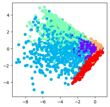
(a)

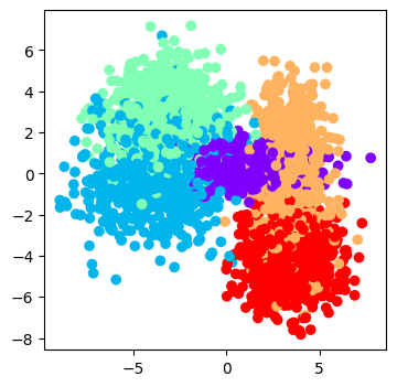
(b)

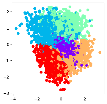
(c)

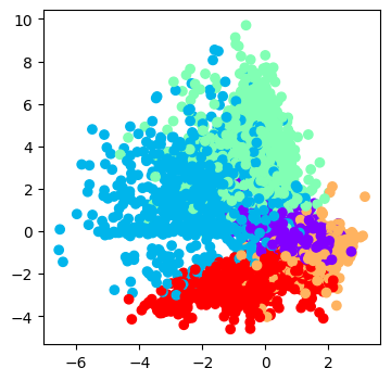
(d)

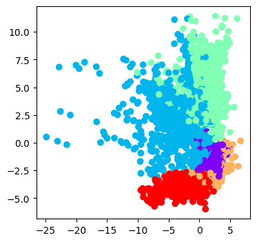
(e)

Figure 1: Bi-modal model with label (colour-coded) and continuous modality in (a) with true latent variables in (b). Inferred latent variables in (c) - (e) with a linear transformation inditerminancy.

Auxiliary labels as modalities.

We construct artificial data following [62], with the latent variables $Z\in\mathbb{R}^{D}$ being conditionally Gaussian having means and variances that depend on an observed index value $X_{2}\in[K]$. More precisely, $p_{\theta}(z|x_{2})=\mathcal{N}(\mu_{x_{2}},\Sigma_{x_{2}})$, where $\mu_{c}\sim\otimes\leavevmode\nobreak\ \mathcal{U}(-5,5)$ and $\Sigma_{c}=\text{diag}(\Lambda_{c})$, $\Lambda_{c}\sim\otimes\leavevmode\nobreak\ \mathcal{U}(0.5,3)$ iid for $c\in[K]$. The marginal distribution over the labels is uniform $\mathcal{U}([K])$ so that the prior density $p_{\theta}(z)=\int_{[K]}p_{\theta}(z|x_{2})p_{\theta}(x_{2})\mathrm{d}x_{2}$ becomes a Gaussian mixture. We choose an injective decoding function $f_{1}\colon\mathbb{R}^{D}\to\mathbb{R}^{D_{1}}$, $D\leq D_{1}$, as a composition of MLPs with LeakyReLUs and full rank weight matrices having monotonically increasing row dimensions [63] and with iid randomly sampled entries. We assume $X_{1}|Z\sim\mathcal{N}(f_{1}(Z),\sigma^{2}\operatorname{I})$. We set $\sigma=0.1$, $D=D_{1}=2$, and $f_{1}$ has a single hidden layer of size $D_{1}=2$. One realisation of bi-modal data $X$, the true latent variable $Z$, as well as inferred latent variables for a selection of different bounds and aggregation schemes, are shown in Figure 1, with more examples given in Figures 6 and 7. Results over multiple repetitions in Table 7 indicate that both a tighter variational bound and more flexible aggregation schemes improve the identifiability of the latent variables and the log-likelihood as estimated using importance sampling with $64$ particles.

Multiple modalities.

Considering the same generative model for $Z$ with a Gaussian mixture prior, suppose now that instead of observing the auxiliary label, we observe multiple modalities $X_{s}\in\mathbb{R}^{D_{s}}$, $X_{s}|Z\sim\mathcal{N}(f_{s}(Z),\sigma^{2}\operatorname{I})$, for injective MLPs $f_{s}$ constructed as above, with $D=10$, $D_{s}=25$, $\sigma=0.5$ and $K=M=5$. We consider a semi-supervised setting where modalities are missing completely at random, as in [145], with a missing rate $\eta$ as the sample average of $\frac{1}{|\mathcal{M}|}\sum_{s\in\mathcal{M}}(1-M_{s})$. Our bound and the suggested permutation-invariant aggregation schemes can naturally accommodate this partially observed setting, see Appendix I for details. Table 2 shows that using the new variational bound improves the log-likelihood and the identifiability of the latent representation. Furthermore, using learnable aggregation schemes benefits both variational bounds.

Table 2: Partially observed ($\eta=0.5$) non-linear identifiable model with $5$ modalities: The first four rows use a fixed standard Gaussian prior, while the last four rows use a Gaussian mixture prior with $5$ components. Mean and standard deviation over 4 repetitions.

	Our bound			Mixture
Aggregation	LLH	Lower Bound	MCC	LLH	Lower Bound	MCC
PoE	-250.9 (5.19)	-256.1 (5.43)	0.94 (0.015)	-288.4 (8.53)	-328.8 (9.17)	0.93 (0.018)
MoE	-250.1 (4.77)	-255.3 (4.90)	0.92 (0.022)	-286.2 (7.63)	-325.1 (8.03)	0.90 (0.019)
SumPooling	-249.6 (4.85)	-253.1 (4.84)	0.95 (0.016)	-275.6 (7.35)	-317.7 (8.72)	0.92 (0.031)
SelfAttention	-249.7 (4.83)	-253.1 (4.84)	0.95 (0.014)	-275.5 (7.45)	-317.6 (8.68)	0.93 (0.022)
SumPooling	-247.3 (4.23)	-251.9 (4.31)	0.95 (0.009)	-269.6 (7.42)	-311.5 (8.47)	0.94 (0.018)
SelfAttention	-247.5 (4.22)	-252.1 (4.21)	0.95 (0.013)	-269.9 (6.06)	-311.6 (7.72)	0.93 (0.022)
SumPoolingMixture	-244.8 (4.44)	-249.5 (5.84)	0.95 (0.011)	-271.9 (6.54)	-313.4 (7.30)	0.93 (0.021)
SelfAttentionMixture	-245.4 (4.55)	-248.2 (4.80)	0.96 (0.010)	-270.3 (5.96)	-312.1 (7.61)	0.94 (0.016)

5.3 MNIST-SVHN-Text

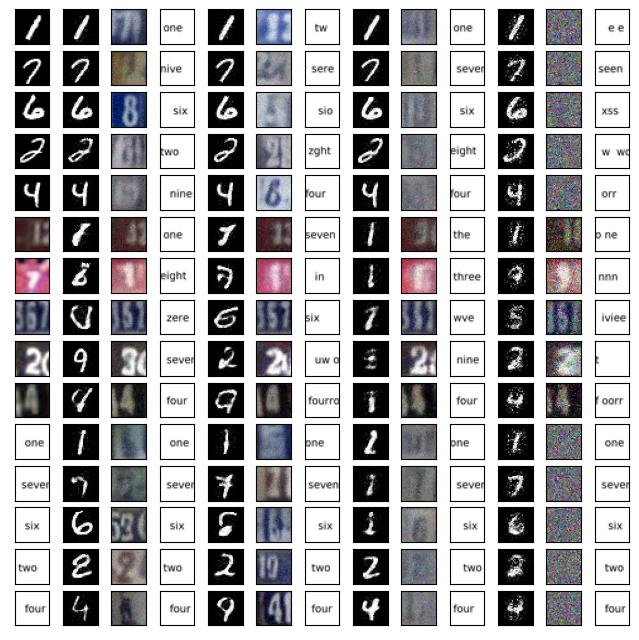
(a)

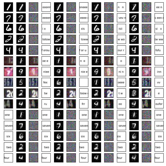
(b)

Figure 10: Conditional generation for different aggergation schemes and bounds and shared latent variables. The first column is the conditioned modality. The next three columns are the generated modalities using a SumPooling aggregation, followed by the three columns for a SelfAttention aggregation, followed by PoE+ and lastly MoE+.

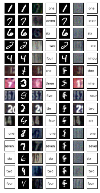
(a)

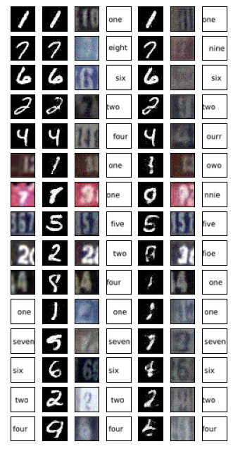
(b)

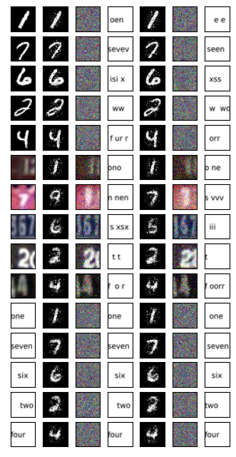
(c)

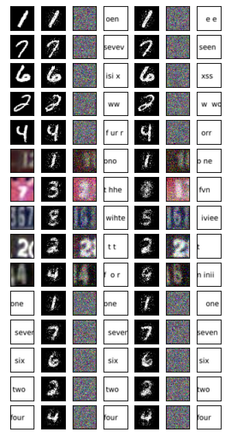
(d)

Figure 11: Conditional generation for different $\beta$ parameters. The first column is the conditioned modality. The next three columns are the generated modalities using a SumPooling aggregation, followed by the three columns for a PoE+ scheme.

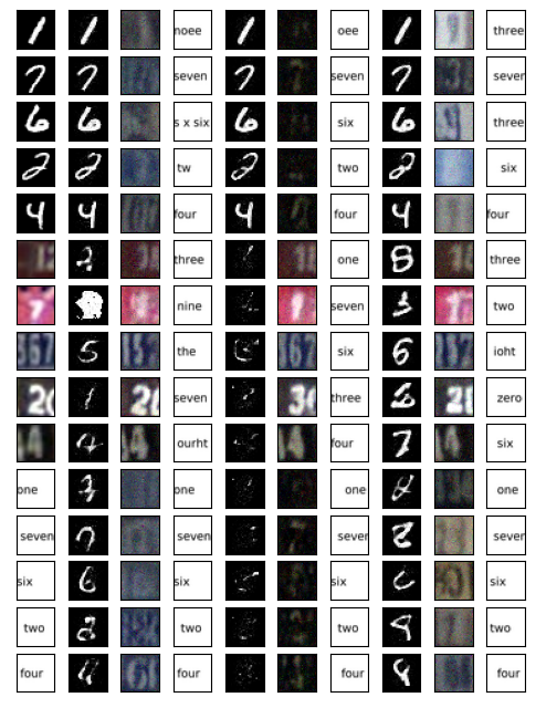
(a)

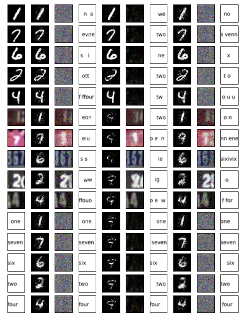
(b)

Figure 12: Conditional generation for permutation-equivariant schemes and private latent variable constraints. The first column is the conditioned modality. The next three columns are the generated modalities using a SumPooling aggregation, followed by the three columns for a SelfAttention scheme and a PoE model.

Following previous work [114, 115, 56], we consider a tri-modal dataset based on augmenting the MNIST-SVHN dataset [110] with a text-based modality comprised of the string with the English name of the digit at different starting positions. Herein, SVHN consists of relatively noisy images, whilst MNIST and text are clearer modalities. Multi-modal VAEs have been shown to exhibit differing performances relative to their multi-modal coherence, latent classification accuracy or test log-likelihood, see Appendix L for definitions. Previous works often differ in their hyperparameters, from neural network architectures, latent space dimensions, priors and likelihood families, modality-specific likelihood weightings, fixed decoder variances, etc. However, we have chosen the same hyperparameters for all models, thereby providing a clearer disentanglement of how either the variational objective or the aggregation scheme affect different multi-modal evaluation measures. In particular, we consider multi-modal generative models with (i) shared latent variables and (ii) private and shared latent variables. As an additional benchmark we also consider PoE or MoE schemes (denoted PoE+, resp., MoE+) with additional neural network layers in their modality-specific encoding functions so that the number of parameters matches or exceeds those of the introduced permutation-invariant models, see Appendix P.5 for details. For models without private latent variables, estimates of the test log-likelihoods in Table 3 suggest that our bound improves the log-likelihood across different aggregation schemes for all modalities and differnet $\beta$s (Table 9), with similar results for permutation-equivariant schemes, except for a Self-Attention model. Furthermore, more flexible fusion schemes yield higher log-likelihoods for both bounds. We provide qualitative results for the reconstructed modalities in Figures 10 - 12. We believe that the clearest observation here is that realistic cross-generation of the SVHN modality is challenging for the mixture-based bound with all aggregation schemes. In contrast, our bound, particularly when combined with the learnable aggregation schemes, improves the cross-generation of SVHN. No bound or aggregation scheme performs best across all modalities by the generative coherence measures (see Table 4 for uni-modal inputs, Table 10 for bi-modal ones and Tables 11 - 14 for models with private latent variables and different $\beta$s). Overall, our bound is slightly more coherent for cross-generating SVHN or Text, but less coherent for MNIST. Furthermore, mixture based bounds tend to improve the unsupervised latent classifcation accuracy across different fusion approaches and modalities, see Table 15. To provide complementary insights into the trade-offs for the different bounds and fusion schemes, we consider a multi-modal rate-distortion evaluation in Figure 2. Ignoring MoE where reconstructions are similar, observe that our bound improves the full reconstruction, with higher full rates, and across various fusion schemes. In contrast, mixture-based bounds yield improved cross-reconstructions for all aggregation models, with increased cross-rates terms. Flexible permutation-invariant architectures for our bound improve the full reconstruction, even at lower full rates.

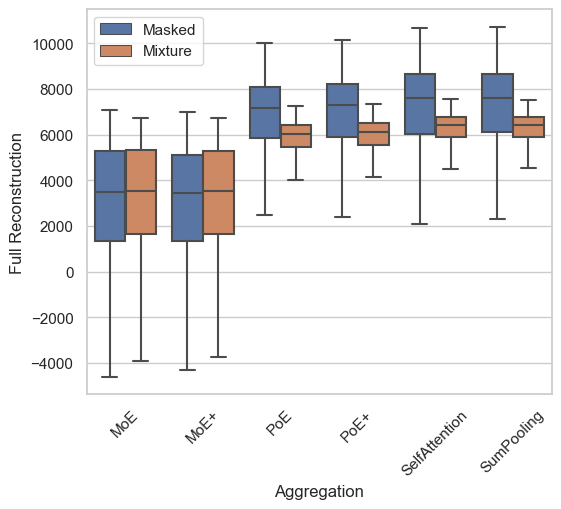
(a)

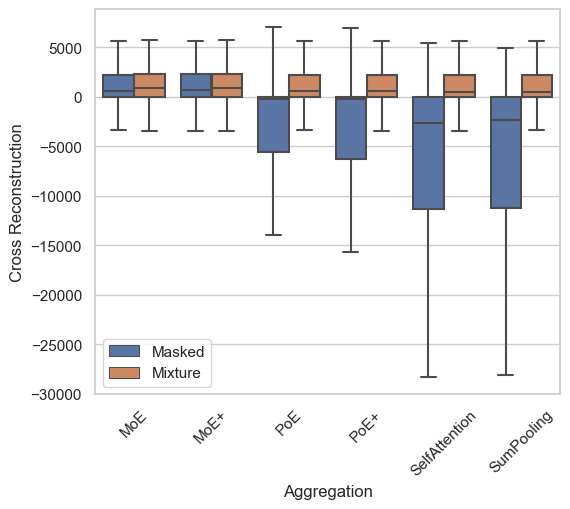
(b)

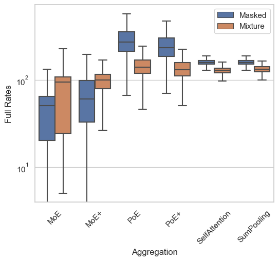
(c)

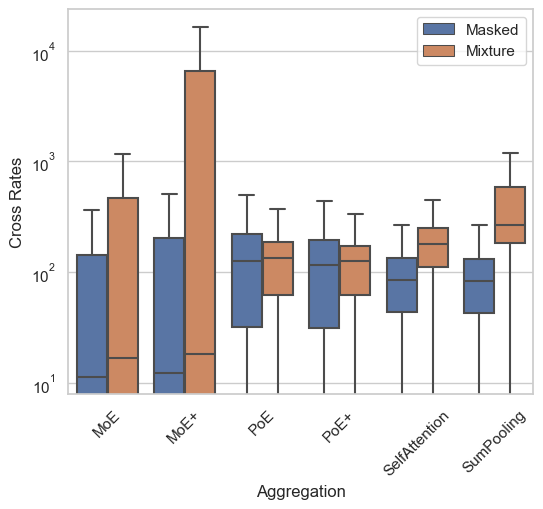
(d)

Figure 2: Rate and distortion terms for MNIST-SVHN-Text with shared latent variables ($\beta=1$).

Table 3: Test log-likelihood estimates for the joint data (M+S+T) and marginal data (importance sampling with 512 particles). The first part of the table is based on the same generative model with shared latent variable $Z\in\mathbb{R}^{40}$, while the second part of the table is based on a restrictive generative model with a shared latent variable $Z^{\prime}\in\mathbb{R}^{10}$ and modality-specific latent variables $\tilde{Z}_{s}\in\mathbb{R}^{10}$.

	Our bound				Mixture bound
Aggregation	M+S+T	M	S	T	M+S+T	M	S	T
PoE+	6872 (9.62)	2599 (5.6)	4317 (1.1)	-9 (0.2)	5900 (10)	2449 (10.4)	3443 (11.7)	-19 (0.4)
PoE	6775 (54.9)	2585 (18.7)	4250 (8.1)	-10 (2.2)	5813 (1.2)	2432 (11.6)	3390 (17.5)	-19 (0.1)
MoE+	5428 (73.5)	2391 (104)	3378 (92.9)	-74 (88.7)	5420 (60.1)	2364 (33.5)	3350 (58.1)	-112 (133.4)
MoE	5597 (26.7)	2449 (7.6)	3557 (26.4)	-11 (0.1)	5485 (4.6)	2343 (1.8)	3415 (5.0)	-17 (0.4)
SumPooling	7056 (124)	2478 (9.3)	4640 (114)	-6 (0.0)	6130 (4.4)	2470 (10.3)	3660 (1.5)	-16 (1.6)
SelfAttention	7011 (57.9)	2508 (18.2)	4555 (38.1)	-7 (0.5)	6127 (26.1)	2510 (12.7)	3621 (8.5)	-13 (0.2)
PoE+	6549 (33.2)	2509 (7.8)	4095 (37.2)	-7 (0.2)	5869 (29.6)	2465 (4.3)	3431 (8.3)	-19 (1.7)
SumPooling	6337 (24.0)	2483 (9.8)	3965 (16.9)	-6 (0.2)	5930 (23.8)	2468 (16.8)	3491 (18.3)	-7 (0.1)
SelfAttention	6662 (20.0)	2516 (8.8)	4247 (31.2)	-6 (0.4)	6716 (21.8)	2430 (26.9)	4282 (49.7)	-27 (1.1)

Table 4: Conditional coherence with shared latent variables and uni-modal inputs. The letters on the second line represent the generated modality based on the input modalities on the line below it.

Our bound									Mixture bound
	M			S			T			M			S			T
Aggregation	M	S	T	M	S	T	M	S	T	M	S	T	M	S	T	M	S	T
PoE	0.97	0.22	0.56	0.29	0.60	0.36	0.78	0.43	1.00	0.96	0.83	0.99	0.11	0.57	0.10	0.44	0.39	1.00
PoE+	0.97	0.15	0.63	0.24	0.63	0.42	0.79	0.35	1.00	0.96	0.83	0.99	0.11	0.59	0.11	0.45	0.39	1.00
MoE	0.96	0.80	0.99	0.11	0.59	0.11	0.44	0.37	1.00	0.94	0.81	0.97	0.10	0.54	0.10	0.45	0.39	1.00
MoE+	0.93	0.77	0.95	0.11	0.54	0.10	0.44	0.37	0.98	0.94	0.80	0.98	0.10	0.53	0.10	0.45	0.39	1.00
SumPooling	0.97	0.48	0.87	0.25	0.72	0.36	0.73	0.48	1.00	0.97	0.86	0.99	0.10	0.63	0.10	0.45	0.40	1.00
SelfAttention	0.97	0.44	0.79	0.20	0.71	0.36	0.61	0.43	1.00	0.97	0.86	0.99	0.10	0.63	0.11	0.45	0.40	1.00

6 Conclusion

Limitations.

A drawback of our bound is that computing a gradient step is more expensive as it requires drawing samples from two encoding distributions. Similarly, learning aggregation functions is more computationally expensive compared to fixed schemes. Mixture-based bounds might be preferred if one is interested primarily in cross-modal reconstructions.

Outlook.

Using modality-specific encoders to learn features and aggregating them with a permutation-invariant function is clearly not the only choice for building multi-modal encoding distributions. However, it allows us to utilize modality-specific architectures for the encoding functions. Alternatively, our bounds could also be used, e.g., when multi-modal transformer architectures [141] encode a distribution on a shared latent space. Our approach applies to general prior densities if we can compute its cross-entropy relative to the multi-modal encoding distributions. An extension would be to apply it with more flexible prior distributions, e.g., as specified via score-based generative models [124]. The ideas in this work might also be of interest for other approaches that require flexible modeling of conditional distributions, such as in meta-learning with Neural processes.

.tocmtappendix mtchapternone mtappendixsubsection

Appendix A Multi-modal distribution matching

Proof of Proposition 2.

Our proof extends the arguments in [138]. Observe first that for any $\mathcal{S}\subset\mathcal{M}$, the encoding distribution is marginally consistent in the sense that it holds that

$$\int_{\mathsf{X}_{\setminus\mathcal{S}}}q_{\phi}(z,x)\mathrm{d}x_{\setminus\mathcal{S}}=\int_{\mathsf{X}_{\setminus\mathcal{S}}}p_{d}(x_{\mathcal{S}})q_{\phi}(x_{\setminus\mathcal{S}}|z,x_{\mathcal{S}})q_{\phi}(z|x_{\mathcal{S}})\mathrm{d}x_{\setminus\mathcal{S}}=p_{d}(x_{\mathcal{S}})q_{\phi}(z|x_{\mathcal{S}}).$$

Consequently,

$$\mathsf{K}\mathsf{L}(q_{\phi}(z,x)|p_{\theta}(z,x))$$

$$= \int_{\mathsf{X}\times\mathsf{Z}}\log\frac{p_{d}(x_{\mathcal{S}})p_{d}(x_{\setminus\mathcal{S}}|x_{\mathcal{S}})q_{\phi}(z|x)q_{\phi}(z|x_{\mathcal{S}})}{p_{\theta}(z)p_{\theta}(x_{\mathcal{S}}|z)p_{\theta}(x_{\setminus\mathcal{S}}|z)q_{\phi}(z|x_{\mathcal{S}})}p_{d}(x)q_{\phi}(z|x)\mathrm{d}x\mathrm{d}z$$

$$= \int_{\mathsf{X}_{\mathcal{S}}\times\mathsf{Z}}\log\frac{p_{d}(x_{\mathcal{S}})q_{\phi}(z|x_{\mathcal{S}})}{p_{\theta}(z)p_{\theta}(x_{\mathcal{S}}|z)}\int_{\mathsf{X}_{\setminus\mathcal{S}}}\left(q_{\phi}(z,x)\mathrm{d}x_{\setminus\mathcal{S}}\right)\mathrm{d}x_{\mathcal{S}}\mathrm{d}z$$

$$+\int_{\mathsf{X}\times\mathsf{Z}}p_{d}(x)q_{\phi}(z|x)\log\frac{p_{d}(x_{\setminus\mathcal{S}}|x_{\mathcal{S}})q_{\phi}(z|x)}{p_{\theta}(x_{\setminus\mathcal{S}}|z)q_{\phi}(z|x_{\mathcal{S}})}\mathrm{d}x\mathrm{d}z$$

$$= \int_{\mathsf{X}_{\mathcal{S}}\times\mathsf{Z}}p_{d}(x_{\mathcal{S}})q_{\phi}(z|x_{\mathcal{S}})\log\frac{q_{\phi}(z|x_{\mathcal{S}})}{p_{\theta}(z)p_{\theta}(x_{\mathcal{S}}|z)}\mathrm{d}x_{\mathcal{S}}\mathrm{d}z-\mathcal{H}(p_{d}(x_{\mathcal{S}}))$$

$$+\int_{\mathsf{X}\times\mathsf{Z}}p_{d}(x)q_{\phi}(z|x)\log\frac{q_{\phi}(z|x)}{p_{\theta}(x_{\setminus\mathcal{S}}|z)q_{\phi}(z|x_{\mathcal{S}})}\mathrm{d}x\mathrm{d}z-\mathcal{H}(p_{d}(x_{\setminus\mathcal{S}}|x_{\mathcal{S}})).$$

The claim follows by the chain rule for the entropy. ∎

Following the same arguments as for uni-modal VAEs, this establishes a lower bound on the log-likelihood.

Corollary (Tight lower bound on multi-modal log-likelihood).

For any modality mask $\mathcal{S}$, we have

$$\int p_{d}(x)\left[\mathcal{L}_{\mathcal{S}}(x_{\mathcal{S}},\theta,\phi,1)+\mathcal{L}_{\setminus\mathcal{S}}(x,\theta,\phi,1)\right]\mathrm{d}x=\int p_{d}(x)\left[\log p_{\theta}(x)-\mathsf{K}\mathsf{L}(q_{\phi}(z|x)|p_{\theta}(z|x))\right]\mathrm{d}x.$$

Proof.

Recall that $q_{\phi}(z,x)=p_{d}(x)q_{\phi}(z|x)$. Proposition A implies then that

$$\int p_{d}(x)\left[\mathcal{L}_{\mathcal{S}}(x_{\mathcal{S}},\theta,\phi,1)+\mathcal{L}_{\setminus\mathcal{S}}(x,\theta,\phi,1)\right]\mathrm{d}x$$

$$= -\mathsf{K}\mathsf{L}(q_{\phi}(z,x)|p_{\theta}(z,x))-\mathcal{H}(p_{d}(x))$$

$$= -\int p_{d}(x)\int q_{\phi}(z|x)\log q_{\phi}(z|x)-\log p_{\theta}(z,x))\mathrm{d}z\mathrm{d}x$$

$$= \int p_{d}(x)\log p_{\theta}(x)\mathrm{d}x-\int q_{\phi}(z|x)\left(\log p_{\theta}(z|x)-\log q_{\phi}(z|x)\right)\mathrm{d}z\mathrm{d}x.$$

∎

Remark .

Corollary A shows that the variational bound becomes tight if the encoding distribution closely approximates the true posterior distribution. A similar result does not hold for the mixture-based multi-modal bound. Indeed, as shown in [22], there is a gap between the variational bound and the log-likelihood given by the conditional entropies that cannot be reduced even for flexible encoding distributions. Moreover, our bound can be tight for an arbitrary number of modalities. In contrast, [22] show that for mixture-based bounds, this variational gap increases with each additional modality, if the new modality is ’sufficiently diverse’.

Proposition (Marginal and conditional distribution matching).

For any $\mathcal{S}\in\mathcal{P}(\mathcal{M})$, we have

$$\int p_{d}(x_{\mathcal{S}})\mathcal{L}_{\mathcal{S}}(x_{\mathcal{S}},\theta,\phi)\mathrm{d}x_{\mathcal{S}}+\mathcal{H}(p_{d}(x_{\mathcal{S}}))$$

$$= -\mathsf{K}\mathsf{L}(q_{\phi}(z,x_{\mathcal{S}})|p_{\theta}(z,x_{\mathcal{S}})) \mathsf{Z}\mathsf{X}_{\text{marginal}}$$ ()

$$= -\mathsf{K}\mathsf{L}(p_{d}(x_{\mathcal{S}})|p_{\theta}(x_{\mathcal{S}}))-\int p_{d}(x_{\mathcal{S}})\mathsf{K}\mathsf{L}(q_{\phi}(z|x_{\mathcal{S}})|p_{\theta}(z|x_{\mathcal{S}}))\mathrm{d}x_{\mathcal{S}} \mathsf{X}_{\text{marginal}}$$ ()

$$= -\mathsf{K}\mathsf{L}(q_{\phi,\mathcal{S}}^{\text{agg}}(z)|p_{\theta}(z))-\int q_{\phi,\mathcal{S}}^{\text{agg}}(z)\mathsf{K}\mathsf{L}(q^{\star}(x_{\mathcal{S}}|z)|p_{\theta}(x_{\mathcal{S}}|z))\mathrm{d}x_{\mathcal{S}}, \mathsf{Z}_{\text{marginal}}$$ ()

where $q_{\phi,\mathcal{S}}^{\text{agg}}(z)=\int p_{d}(x_{\mathcal{S}})q_{\phi}(z|x_{\mathcal{S}})\mathrm{d}x_{\mathcal{S}}$ is the aggregated prior [87] restricted on modalities from $\mathcal{S}$ and $q^{\star}(x_{\mathcal{S}}|z)=q_{\phi}(x_{\mathcal{S}},z)/q_{\phi}^{\text{agg}}(z)$. Moreover, for fixed $x_{\mathcal{S}}$,

$$\int p_{d}(x_{\setminus\mathcal{S}}|x_{\mathcal{S}})\mathcal{L}_{\setminus\mathcal{S}}(x,\theta,\phi)\mathrm{d}x_{\setminus\mathcal{S}}+\mathcal{H}(p_{d}(x_{\setminus\mathcal{S}}|x_{\mathcal{S}}))$$

$$= -\mathsf{K}\mathsf{L}\left(q_{\phi}(z|x)p_{d}(x_{\setminus\mathcal{S}}|x_{\mathcal{S}})\big{|}p_{\theta}(x_{\setminus\mathcal{S}}|z)q_{\phi}(z|x_{\mathcal{S}})\right) \mathsf{Z}\mathsf{X}_{\text{conditional}}$$ ()

$$= -\mathsf{K}\mathsf{L}(p_{d}(x_{\setminus\mathcal{S}}|x_{\mathcal{S}})|p_{\theta}(x_{\setminus\mathcal{S}}|x_{\mathcal{S}})) \mathsf{X}_{\text{conditional}}$$ ()

$$-\int p_{d}(x_{\setminus\mathcal{S}}|x_{\mathcal{S}})\left(\mathsf{K}\mathsf{L}(q_{\phi}(z|x)|p_{\theta}(z|x))+\int q_{\phi}(z|x)\log\frac{q_{\phi}(z|x_{\mathcal{S}})}{p_{\theta}(z|x_{\mathcal{S}})}\mathrm{d}z\right)\mathrm{d}x_{\setminus\mathcal{S}}$$

$$= -\mathsf{K}\mathsf{L}(q_{\phi,\setminus\mathcal{S}}^{\text{agg}}(z|x_{\mathcal{S}})|q_{\phi}(z|x_{\mathcal{S}}))-\int q_{\phi,\setminus\mathcal{S}}^{\text{agg}}(z|x_{\mathcal{S}})\left(\mathsf{K}\mathsf{L}(q^{\star}(x_{\setminus\mathcal{S}}|z,x_{\mathcal{S}})|p_{\theta}(x_{\mathcal{S}}|z))\right)\mathrm{d}z,$$

where $q_{\phi,\setminus\mathcal{S}}^{\text{agg}}(z|x_{\mathcal{S}})=\int p_{d}(x_{\setminus\mathcal{S}}|x_{\mathcal{S}})q_{\phi}(z|x)\mathrm{d}x_{\setminus\mathcal{S}}$ can be seen as an aggregated encoder conditioned on $x_{\mathcal{S}}$ and $q^{\star}(x_{\setminus\mathcal{S}}|z,x_{\mathcal{S}})=q_{\phi}(z,x_{\setminus\mathcal{S}}|x_{\mathcal{S}})/q^{\text{agg}}_{\phi,\setminus\mathcal{S}}(z|x_{\mathcal{S}})=p_{d}(x_{\setminus\mathcal{S}}|x_{\mathcal{S}})q_{\phi}(z|x)/q^{\text{agg}}_{\phi,\setminus\mathcal{S}}(z|x_{\mathcal{S}})$.

Proof of Proposition A.

The equations for $\mathcal{L}_{\mathcal{S}}(x_{\mathcal{S}})$ are well known for uni-modal VAEs, see for example [150]. To derive similar representations for the conditional bound, note that the first equation ($\mathsf{Z}\mathsf{X}_{\text{conditional}}$) for matching the joint distribution of the latent and the missing modalities conditional on a modality subset follows from the definition of $\mathcal{L}_{\setminus\mathcal{S}}$,

$$\int p_{d}(x_{\setminus\mathcal{S}}|x_{\mathcal{S}})\mathcal{L}_{\setminus\mathcal{S}}(x,\theta,\phi)\mathrm{d}x_{\setminus\mathcal{S}}$$

$$= \int p_{d}(x_{\setminus\mathcal{S}}|x_{\mathcal{S}})\int q_{\phi}(z|x)\left[\log p_{\theta}(x_{\setminus\mathcal{S}}|z)-\log q_{\phi}(z|x)+\log q_{\phi}(z|x_{\mathcal{S}}))\right]\mathrm{d}z\mathrm{d}x_{\setminus\mathcal{S}}$$

$$= \int p_{d}(x_{\setminus\mathcal{S}}|x_{\mathcal{S}})\log p_{d}(x_{\setminus\mathcal{S}}|x_{\mathcal{S}})\mathrm{d}x_{\setminus\mathcal{S}}+\int p_{d}(x_{\setminus\mathcal{S}}|x_{\mathcal{S}})\int q_{\phi}(z|x)\left[\log\frac{p_{\theta}(x_{\setminus\mathcal{S}}|z)q_{\phi}(z|x_{\mathcal{S}}))}{q_{\phi}(z|x)p_{d}(x_{\setminus\mathcal{S}}|x_{\mathcal{S}})}\right]\mathrm{d}z\mathrm{d}x_{\setminus\mathcal{S}}$$

$$= -\mathcal{H}(p_{d}(x_{\setminus\mathcal{S}}|x_{\mathcal{S}}))-\mathsf{K}\mathsf{L}\left(q_{\phi}(z|x)p_{d}(x_{\setminus\mathcal{S}}|x_{\mathcal{S}})\big{|}p_{\theta}(x_{\setminus\mathcal{S}}|z)q_{\phi}(z|x_{\mathcal{S}})\right).$$

To obtain the second representation ($\mathsf{X}_{\text{conditional}}$) for matching the conditional distributions in the data space, observe that $p_{\theta}(x_{\setminus\mathcal{S}}|x_{\mathcal{S}},z)=p_{\theta}(x_{\setminus\mathcal{S}}|z)$ and consequently,

$$-\int p_{d}(x_{\setminus\mathcal{S}}|x_{\mathcal{S}})\mathcal{L}_{\setminus\mathcal{S}}(x,\theta,\phi)\mathrm{d}x_{\setminus\mathcal{S}}-\mathcal{H}(p_{d}(x_{\setminus\mathcal{S}}|x_{\mathcal{S}}))$$

$$= \int p_{d}(x_{\setminus\mathcal{S}}|x_{\mathcal{S}})q_{\phi}(z|x)\log\frac{p_{d}(x_{\setminus\mathcal{S}}|x_{\mathcal{S}})q_{\phi}(z|x)}{p_{\theta}(x_{\setminus\mathcal{S}}|z)q_{\phi}(z|x_{\mathcal{S}})}\mathrm{d}z\mathrm{d}x_{\setminus\mathcal{S}}$$

$$= \int p_{d}(x_{\setminus\mathcal{S}}|x_{\mathcal{S}})q_{\phi}(z|x)\log\frac{p_{d}(x_{\setminus\mathcal{S}}|x_{\mathcal{S}})q_{\phi}(z|x)p_{\theta}(z|x_{\mathcal{S}})}{p_{\theta}(x_{\setminus\mathcal{S}}|z)p_{\theta}(z|x_{\mathcal{S}})q_{\phi}(z|x_{\mathcal{S}})}\mathrm{d}z\mathrm{d}x_{\setminus\mathcal{S}}$$

$$= \int p_{d}(x_{\setminus\mathcal{S}}|x_{\mathcal{S}})q_{\phi}(z|x)\log\frac{p_{d}(x_{\setminus\mathcal{S}}|x_{\mathcal{S}})q_{\phi}(z|x)p_{\theta}(z|x_{\mathcal{S}})}{p_{\theta}(x_{\setminus\mathcal{S}}|z,x_{\mathcal{S}})p_{\theta}(z|x_{\mathcal{S}})q_{\phi}(z|x_{\mathcal{S}})}\mathrm{d}z\mathrm{d}x_{\setminus\mathcal{S}}$$

$$= \int p_{d}(x_{\setminus\mathcal{S}}|x_{\mathcal{S}})q_{\phi}(z|x)\log\frac{p_{d}(x_{\setminus\mathcal{S}}|x_{\mathcal{S}})q_{\phi}(z|x)p_{\theta}(z|x_{\mathcal{S}})}{p_{\theta}(x_{\setminus\mathcal{S}}|x_{\mathcal{S}})p_{\theta}(z|x_{\mathcal{S}},x_{\setminus\mathcal{S}})q_{\phi}(z|x_{\mathcal{S}})}\mathrm{d}z\mathrm{d}x_{\setminus\mathcal{S}}$$

$$= \mathsf{K}\mathsf{L}(p_{d}(x_{\setminus\mathcal{S}}|x_{\mathcal{S}})|p_{\theta}(x_{\setminus\mathcal{S}}|x_{\mathcal{S}}))+\int p_{d}(x_{\setminus\mathcal{S}}|x_{\mathcal{S}})\int q_{\phi}(z|x)\left[\log\frac{q_{\phi}(z|x)}{p_{\theta}(z|x)}+\log\frac{p_{\theta}(z|x_{\mathcal{S}})}{q_{\phi}(z|x_{\mathcal{S}})}\right]\mathrm{d}z\mathrm{d}x_{\setminus\mathcal{S}}.$$

Lastly, the representation () for matching the distributions in the latent space given a modality subset follows by recalling that

$$p_{d}(x_{\setminus\mathcal{S}}|x_{\mathcal{S}})q_{\phi}(z|x)=q^{\text{agg}}_{\phi,\setminus\mathcal{S}}(z|x_{\mathcal{S}})q^{\star}(x_{\setminus\mathcal{S}}|z,x_{\mathcal{S}})$$

and consequently,

$$-\int p_{d}(x_{\setminus\mathcal{S}}|x_{\mathcal{S}})\mathcal{L}_{\setminus\mathcal{S}}(x,\theta,\phi)\mathrm{d}x_{\setminus\mathcal{S}}-\mathcal{H}(p_{d}(x_{\setminus\mathcal{S}}|x_{\mathcal{S}}))$$

$$= \int p_{d}(x_{\setminus\mathcal{S}}|x_{\mathcal{S}})q_{\phi}(z|x)\log\frac{p_{d}(x_{\setminus\mathcal{S}}|x_{\mathcal{S}})q_{\phi}(z|x)}{p_{\theta}(x_{\setminus\mathcal{S}}|z)q_{\phi}(z|x_{\mathcal{S}})}\mathrm{d}z\mathrm{d}x_{\setminus\mathcal{S}}$$

$$= \int q^{\text{agg}}_{\phi,\setminus\mathcal{S}}(z|x_{\mathcal{S}})q^{\star}(x_{\setminus\mathcal{S}}|z,x_{\mathcal{S}})\log\frac{q^{\text{agg}}_{\phi,\setminus\mathcal{S}}(z|x_{\mathcal{S}})q^{\star}(x_{\setminus\mathcal{S}}|z,x_{\mathcal{S}})}{p_{\theta}(x_{\setminus\mathcal{S}}|z)q_{\phi}(z|x_{\mathcal{S}})}\mathrm{d}z\mathrm{d}x_{\setminus\mathcal{S}}$$

$$= \mathsf{K}\mathsf{L}(q_{\phi,\setminus\mathcal{S}}^{\text{agg}}(z|x_{\mathcal{S}})|q_{\phi}(z|x_{\mathcal{S}}))-\int q_{\phi,\setminus\mathcal{S}}^{\text{agg}}(z|x_{\mathcal{S}})\left(\mathsf{K}\mathsf{L}(q^{\star}(x_{\setminus\mathcal{S}}|z,x_{\mathcal{S}})|p_{\theta}(x_{\mathcal{S}}|z))\right)\mathrm{d}z.$$

∎

Remark (Prior-hole problem and Bayes or conditional consistency).

In the uni-modal setting, the mismatch between the prior and the aggregated prior can be large and can lead to poor unconditional generative performance, because this would lead to high-probability regions under the prior that have not been trained due to their small mass under the aggregated prior [48, 103]. Equation ($\mathsf{Z}_{\text{marginal}}$) extents this to the multi-modal case and we expect that unconditional generation can be poor if this mismatch is large. Moreover, () extends this conditioned on some modality subset and we expect that cross-generation for $x_{\setminus\mathcal{S}}$ conditional on $x_{\mathcal{S}}$ can be poor if the mismatch between $q_{\phi,\setminus\mathcal{S}}^{\text{agg}}(z|x_{\mathcal{S}})$ and $q_{\phi}(z|x_{\mathcal{S}})$ is large for $x_{\mathcal{S}}\sim p_{d}$, because high-probability regions under $q_{\phi}(z|x_{\mathcal{S}})$ will not have been trained - via optimizing $\mathcal{L}_{\setminus\mathcal{S}}(x)$ - to model $x_{\setminus\mathcal{S}}$ conditional on $x_{\mathcal{S}}$, due to their small mass under $q_{\phi,\setminus\mathcal{S}}^{\text{agg}}(z|x_{\mathcal{S}})$. The mismatch will vanish when the encoders are consistent and correspond to a single Bayesian model where they approximate the true posterior distributions.

Appendix B Meta-learning and Neural processes

Meta-learning.

We consider a standard meta-learning setup but use slightly non-standard notations to remain consistent with notations used in other parts of this work. We consider a compact input or covariate space $\mathcal{A}$ and output space $\mathcal{X}$. Let $\mathcal{D}=\cup_{M=1}^{\infty}(\mathcal{A}\times\mathcal{X})^{M}$ be the collection of all input-output pairs. In meta-learning, we are given a meta-dataset, i.e., a collection of elements from $\mathcal{D}$. Each individual data set $D=(a,x)=D_{c}\cup D_{t}\in\mathcal{D}$ is called a task and split into a context set $D_{c}=(a_{c},x_{c})$, and target set $D_{t}=(a_{t},x_{t})$. We aim to predict the target set from the context set. Consider, therefore, the prediction map

$$\pi\colon D_{c}=(a_{c},x_{c})\mapsto p(x_{t}|a_{t},D_{c})=p(x_{t},x_{c}|a_{t},a_{c})/p(x_{c}|a_{c}),$$

mapping each context data set to the predictive stochastic process conditioned on $D_{c}$.

Variational lower bounds for Neural processes.

Latent Neural processes [34, 31] approximate this prediction map by using a latent variable model with parameters $\theta$ in the form of

$$z\sim p_{\theta},\leavevmode\nobreak\ p_{\theta}(x_{t}|a_{t},z)=\prod_{(a,x)\in D_{t}}p_{\epsilon}(x-f_{\theta}(a,z))$$

for a prior $p_{\theta}$, decoder $f_{\theta}$ and a parameter free density $p_{\epsilon}$. The model is then trained by (approximately) maximizing a lower bound on $\log p_{\theta}(x_{t}|a_{t},a_{c},x_{c})$. Note that for an encoding density $q_{\phi}$, we have that

$$\log p_{\theta}(x_{t}|a_{t},a_{c},x_{x})=\int q_{\phi}(z|x,a)\log p_{\theta}(x_{t}|a_{t},z)\mathrm{d}z-\mathsf{K}\mathsf{L}(q_{\phi}(z|a,x)|p_{\theta}(z|a_{c},x_{c})).$$

Since the posterior distribution $p_{\theta}(z|a_{c},x_{c})$ is generally intractable, one instead replaces it with a variational approximation or learned conditional prior $q_{\phi}(z|a_{c},x_{c})$, and optimizes the following objective

$$\mathcal{L}^{\text{LNP}}_{\setminus\mathcal{C}}(x,a)=\int q_{\phi}(z|x,a)\log p_{\theta}(x_{t}|a_{t},z)\mathrm{d}z-\mathsf{K}\mathsf{L}(q_{\phi}(z|a,x)|q_{\phi}(z|a_{c},x_{c})).$$

Note that this objective coincides with $\mathcal{L}_{\setminus\mathcal{C}}$ conditioned on the covariate values $a$ and where $\mathcal{C}$ comprises the indices of the data points that are part of the context set.

Using this variational lower bound can yield subpar performance compared to other biased log-likelihood objectives [64, 31], possibly because the variational approximation $q_{\phi}(z|a_{c},x_{c})$ needs not to be close the posterior distribution $p_{\theta}(z|a_{c},x_{c})$. It would therefore be interesting to analyze in future work if one can alleviate such issues if one optimizes additionally the variational objective corresponding to $\mathcal{L}_{\mathcal{C}}$, i.e.,

$$\mathcal{L}^{\text{LNP}}_{\mathcal{C}}(x_{c},a_{c})=\int q_{\phi}(z|x_{c},a_{c})\log p_{\theta}(x_{c}|a_{c},z)\mathrm{d}z-\mathsf{K}\mathsf{L}(q_{\phi}(z|a_{c},x_{c})|p_{\theta}(z)),$$

as we do in this work for multi-modal generative models. Note that the objective $\mathcal{L}^{\text{LNP}}_{\mathcal{C}}$ alone can be seen as a form of a neural statistician model [27] where $\mathcal{C}$ coincides with the indices of the target set, while a form of the mixture-based bound corresponds to a neural process bound similar to variational homoencoders [45], see also the discussion in [73].

Appendix C Information-theoretic perspective

We recall first that the mutual information on the inference path is given by

$$\operatorname{I}_{q_{\phi}}(X_{\mathcal{S}},Z_{\mathcal{S}})=\int q_{\phi}(x_{\mathcal{S}},z)\log\frac{q_{\phi}(x_{\mathcal{S}},z)}{p_{d}(x_{\mathcal{S}})q_{\phi,\mathcal{S}}^{\text{agg}}(z)}\mathrm{d}z\mathrm{d}x_{\mathcal{S}},$$

where $q_{\phi,\mathcal{S}}^{\text{agg}}(z)=\int p_{d}(x_{\mathcal{S}})q_{\phi}(z|x_{\mathcal{S}})\mathrm{d}x_{\mathcal{S}}$ is the aggregated prior [87]. It can be bounded by standard [11, 4, 3] lower and upper bounds using the rate and distortion:

$$\mathcal{H}_{\mathcal{S}}-D_{\mathcal{S}}\leq\mathcal{H}_{\mathcal{S}}-D_{\mathcal{S}}+\Delta_{1}=\operatorname{I}_{q_{\phi}}(X_{\mathcal{S}},Z_{\mathcal{S}})=R_{\mathcal{S}}-\Delta_{2}\leq R_{\mathcal{S}},$$

with $\Delta_{1}=\int q_{\phi}^{\text{agg}}(z)\mathsf{K}\mathsf{L}(q^{\star}(x_{\mathcal{S}}|z)|p_{\theta}(x_{\mathcal{S}}|z))\mathrm{d}z>0$, $\Delta_{2}=\mathsf{K}\mathsf{L}(q_{\phi,\mathcal{S}}^{\text{agg}}(z)|p_{\theta}(z))>0$ and $q^{\star}(x_{\mathcal{S}}|z)=q_{\phi}(x_{\mathcal{S}},z)/q_{\phi}^{\text{agg}}(z)$.

Moreover, if the bounds in (6) become tight with $\Delta_{1}=\Delta_{2}=0$ in the hypothetical scenario of infinite-capacity decoders and encoders, one obtains $\int p_{d}\mathcal{L}_{\mathcal{S}}=(1-\beta)\operatorname{I}_{q_{\phi}}(X_{\mathcal{S}},Z_{\mathcal{S}})+\mathcal{H}_{\mathcal{S}}$. For $\beta>1$, maximizing $\mathcal{L}_{\mathcal{S}}$ yields an auto-decoding limit that minimizes $\operatorname{I}_{q_{\phi}}(x_{\mathcal{S}},z)$ for which the latent representations do not encode any information about the data, whilst $\beta<1$ yields an auto-encoding limit that maximizes $\operatorname{I}_{q_{\phi}}(X_{\mathcal{S}},Z)$ and for which the data is perfectly encoded and decoded.

To arrive at a similar interpretation for the conditional bound $\mathcal{L}_{\setminus\mathcal{S}}$, recall that we have defined $R_{\setminus\mathcal{S}}=\int p_{d}(x)\mathsf{K}\mathsf{L}(q_{\phi}(z|x)|q_{\phi}(z|x_{\mathcal{S}})\mathrm{d}x$ for a conditional or cross rate term and $D_{\setminus\mathcal{S}}=-\int p_{d}(x)q_{\phi}(z|x)\log p_{\theta}(x_{\setminus\mathcal{S}}|z)\mathrm{d}z\mathrm{d}x$ for the distortion term. Bounds on the conditional mutual information

$$\operatorname{I}_{q_{\phi}}(X_{\setminus\mathcal{S}},Z_{\mathcal{M}}|X_{\mathcal{S}})=\int p_{d}(x_{\mathcal{S}})\mathsf{K}\mathsf{L}(p_{d}(x_{\setminus\mathcal{S}},z|x_{\mathcal{S}}))|p_{d}(x_{\setminus\mathcal{S}}|x_{\mathcal{S}})q_{\phi,\setminus\mathcal{S}}^{\text{agg}}(z|x_{\mathcal{S}}))\mathrm{d}x_{\mathcal{S}}$$

with $q_{\phi,\setminus\mathcal{S}}^{\text{agg}}(z|x_{\mathcal{S}})=\int p_{d}(x_{\setminus\mathcal{S}}|x_{\mathcal{S}})q_{\phi}(z|x)\mathrm{d}x_{\setminus\mathcal{S}}$ can be established as follows.

Proof of Lemma 2.

The proof follows by adapting the arguments in [3]. The law of $X_{\setminus\mathcal{S}}$ and $Z$ conditional on $X_{\mathcal{S}}$ on the encoder path can be written as

$$q_{\phi}(z,x_{\setminus\mathcal{S}}|x_{\mathcal{S}})=p_{d}(x_{\setminus\mathcal{S}}|x_{\mathcal{S}})q_{\phi}(z|x)=q^{\text{agg}}_{\phi,\setminus\mathcal{S}}(z|x_{\mathcal{S}})q^{\star}(x_{\setminus\mathcal{S}}|z,x_{\mathcal{S}})$$

with $q^{\star}(x_{\setminus\mathcal{S}}|z,x_{\mathcal{S}})=q_{\phi}(z,x_{\setminus\mathcal{S}}|x_{\mathcal{S}})/q^{\text{agg}}_{\phi,\setminus\mathcal{S}}(z|x_{\mathcal{S}})$. To prove a lower bound on the conditional mutual information, note that

$$\operatorname{I}_{q_{\phi}}(X_{\setminus\mathcal{S}},Z_{\mathcal{M}}|X_{\mathcal{S}})$$

$$= \int p_{d}(x_{\mathcal{S}})\int q^{\text{agg}}_{\phi,\setminus\mathcal{S}}(z|x_{\mathcal{S}})\int q^{\star}(x_{\setminus\mathcal{S}}|z,x_{\mathcal{S}})\log\frac{q^{\text{agg}}_{\phi,\setminus\mathcal{S}}(z|x_{\mathcal{S}})q^{\star}(x_{\setminus\mathcal{S}}|z,x_{\mathcal{S}})}{q^{\text{agg}}_{\phi,\setminus\mathcal{S}}(z|x_{\mathcal{S}})p_{d}(x_{\setminus\mathcal{S}}|x_{\setminus\mathcal{S}})}\mathrm{d}z\mathrm{d}x_{\setminus\mathcal{S}}\mathrm{d}x_{\mathcal{S}}$$

$$= \int p_{d}(x_{\mathcal{S}})\int q^{\text{agg}}_{\phi,\setminus\mathcal{S}}(z|x_{\mathcal{S}})\left[q^{\star}(x_{\setminus\mathcal{S}}|z,x_{\mathcal{S}})\log p_{\theta}(x_{\setminus\mathcal{S}}|z))+\mathsf{K}\mathsf{L}(q^{\star}(x_{\setminus\mathcal{S}}|z,x_{\mathcal{S}})|p_{\theta}(x_{\setminus\mathcal{S}}|z))\right]\mathrm{d}z\mathrm{d}x_{\mathcal{S}}$$

$$\leavevmode\nobreak\ -\int p_{d}(x_{\mathcal{S}})\int p_{d}(x_{\setminus\mathcal{S}}|x_{\mathcal{S}})\log p_{d}(x_{\setminus\mathcal{S}}|x_{\mathcal{S}})\mathrm{d}x$$

$$= \int p_{d}(x)\int q_{\phi}(z|x)\log p_{\theta}(x_{\setminus\mathcal{S}}|z)\mathrm{d}z\mathrm{d}x-\underbrace{\int p_{d}(x_{\mathcal{S}})\int p_{d}(x_{\setminus\mathcal{S}}|x_{\mathcal{S}})\log p_{d}(x_{\setminus\mathcal{S}}|x_{\mathcal{S}})\mathrm{d}x}_{=-\mathcal{H}_{\setminus\mathcal{S}}=-\mathcal{H}(X_{\setminus\mathcal{S}}|X_{\mathcal{S}})}$$

$$+\underbrace{\int p_{d}(x_{\mathcal{S}})\int q^{\text{agg}}_{\phi,\setminus\mathcal{S}}(z|x_{\mathcal{S}})\mathsf{K}\mathsf{L}(q^{\star}(x_{\setminus\mathcal{S}}|z,x_{\mathcal{S}})|p_{\theta}(x_{\setminus\mathcal{S}}|z))\mathrm{d}x_{\mathcal{S}}}_{=\Delta_{\setminus\mathcal{S},1}\geq 0}$$

$$= \Delta_{\setminus\mathcal{S},1}+D_{\setminus\mathcal{S}}+\mathcal{H}_{\setminus\mathcal{S}}.$$

The upper bound follows by observing that

$$\operatorname{I}_{q_{\phi}}(X_{\setminus\mathcal{S}},Z_{\mathcal{M}}|X_{\mathcal{S}})$$

$$= \int p_{d}(x_{\mathcal{S}})\int p_{d}(x_{\setminus\mathcal{S}}|x_{\setminus})\log\frac{q_{\phi}(z|x)p_{d}(x_{\setminus\mathcal{S}}|x_{\mathcal{S}})}{q^{\text{agg}}_{\phi,\setminus\mathcal{S}}(z|x_{\mathcal{S}})p_{d}(x_{\setminus\mathcal{S}}|x_{\mathcal{S}})}\mathrm{d}z\mathrm{d}x$$

$$= \int p_{d}(x)\mathsf{K}\mathsf{L}(q_{\phi}(z|x)|q_{\phi}(z|x_{\mathcal{S}}))\mathrm{d}x-\underbrace{\int p_{d}(x_{\mathcal{S}})\mathsf{K}\mathsf{L}(q^{\text{agg}}_{\phi,\setminus\mathcal{S}}(z|x_{\mathcal{S}})|q_{\phi}(z|x_{\mathcal{S}}))\mathrm{d}x_{\mathcal{S}}}_{=\Delta_{\setminus\mathcal{S},2}\geq 0}$$

$$= R_{\setminus\mathcal{S}}-\Delta_{\setminus\mathcal{S},2}.$$

∎

Appendix D Optimal variational distributions

The optimal variational density for the mixture-based (1) multi-modal objective,

$$\int p_{d}(\mathrm{d}x)\mathcal{L}_{\mathcal{S}}^{\text{Mix}}(x)= \int p_{d}(x_{\mathcal{S}})\int q_{\phi}(z|x_{\mathcal{S}})\int p_{d}(x_{\setminus\mathcal{S}}|x_{\mathcal{S}})$$

$$\left[\log p_{\theta}(x_{\mathcal{S}}|z)+\log p_{\theta}(x_{\setminus\mathcal{S}}|z)-\beta\log p_{\theta}(z)-\beta\log q_{\phi}(z|x_{\mathcal{S}})\right]\mathrm{d}x_{\setminus\mathcal{S}}\mathrm{d}z\mathrm{d}x_{\mathcal{S}}$$

is attained at

$$q^{\star}(z|x_{\mathcal{S}}) \propto\exp\left(\frac{1}{\beta}\int p_{d}(x_{\setminus\mathcal{S}}|x_{\mathcal{S}})\left[\log p_{\theta}(x_{\mathcal{S}}|z)+\log p_{\theta}(x_{\setminus\mathcal{S}}|z)-\beta\log p_{\theta}(z)\right]\mathrm{d}x_{\setminus\mathcal{S}}\right)$$

$$\propto\tilde{p}_{\beta,\theta}(z|x_{\mathcal{S}})\exp\left(\int p_{d}(x_{\setminus\mathcal{S}}|x_{\mathcal{S}})\log\tilde{p}_{\beta,\theta}(x_{\setminus\mathcal{S}}|z)\mathrm{d}x_{\setminus\mathcal{S}}\right).$$

Appendix E Permutation-invariant architectures

Multi-head attention and masking.

We introduce here a standard multi-head attention [10, 125] mapping $\text{MHA}_{\vartheta}\colon\mathbb{R}^{I\times D_{X}}\times\mathbb{R}^{S\times D_{Y}}\to\mathbb{R}^{I\times D_{Y}}$ given by

$$\text{MHA}_{\vartheta}(X,Y)=W^{O}\begin{bmatrix}\text{Head}^{1}(X,Y,Y),\ldots,\text{Head}^{H}(X,Y,Y)\end{bmatrix},\quad\vartheta=(W_{Q},W_{K},W_{V},W_{O}),$$

with output matrix $W_{O}\in\mathbb{R}^{D_{A}\times D_{Y}}$, projection matrices $W_{Q},W_{K},W_{V}\in\mathbb{R}^{D_{Y}\times D_{A}}$ and

$$\text{Head}^{h}(Q,K,V)=\text{Att}(QW_{Q}^{h},KW_{K}^{h},VW_{V}^{h})\in\mathbb{R}^{I\times D}$$ (8)

where we assume that $D=D_{A}/H\in\mathbb{N}$ is the head size. Here, the dot-product attention function is

$$\text{Att}(Q,K,V)=\sigma(QK^{\top})V,$$

where $\sigma$ is the softmax function applied to each column of $Q$ and $K^{\top}$, respectively.

Masked multi-head attention.

In practice, it is convenient to consider masked multi-head attention models $\text{MMHA}_{\vartheta,M}\colon\mathbb{R}^{I\times D_{X}}\times\mathbb{R}^{T\times D_{Y}}\to\mathbb{R}^{I\times D_{Y}}$ for mask matrix $M\in\{0,1\}^{I\times T}$ that operate on key or value sequences of fixed length $T$ where the $h$-th head (8) is given by

$$\text{Head}^{h}(Q,K,V)=\left[M\odot\sigma(QW_{Q}^{h}(KW_{K}^{h})^{\top})\right]V_{t^{\prime}}W_{V}^{h}\in\mathbb{R}^{T\times D}.$$

Using the softmax kernel function $\text{SM}_{D}(q,k)=\exp(q^{\top}k/\sqrt{D})$, we set

$$\text{MMHA}_{\vartheta,M}(X,Y)_{i}=\sum_{t=1}^{T}\sum_{h=1}^{H}\frac{M_{it}\text{SM}_{D}(W_{h}^{Q}X_{i},W_{h}^{K}Y_{t})}{\sum_{t^{\prime}=1}^{T}M_{it^{\prime}}\text{SM}_{D}(X_{i}W_{h}^{Q},Y_{t^{\prime}}W_{h}^{K})}Y_{t}W^{V}_{h}W_{h}^{O}$$ (9)

which does not depend on $Y_{t}$ if $M_{\cdot t}=0$.

Masked self-attention.

For mask matrix $M=mm^{\top}$ with $m=(1_{\left\{s\in\mathcal{S}\right\}})_{s\in\mathcal{M}}$, we write

$$\text{MHA}_{\vartheta}(Y_{\mathcal{S}},Y_{\mathcal{S}})=\text{MMHA}_{\vartheta,M}(\mathfrak{i}(Y_{\mathcal{S}}),\mathfrak{i}(Y_{\mathcal{S}}))_{\mathcal{S}}.$$

where $\text{MMHA}_{\vartheta,M}$ operates on sequences with fixed length and $\mathfrak{i}(Y_{\mathcal{S}}))_{t}=Y_{t}$ if $t\in\mathcal{S}$ and $0$ otherwise.

LayerNorm and SetNorm.

Let $h\in\mathbb{R}^{T\times D}$ and consider the normalisation

$$\text{N}(h)=\frac{h-\mu(h)}{\sigma(h)}\odot\gamma+\beta$$

where $\mu$ and $\sigma$ standardise the input $h$ by computing the mean, and the variance, respectively, over some axis of $h$, whilst $\gamma$ and $\beta$ define a transformation. LayerNorm [8] standardises inputs over last axis, e.g., $\mu(h)=\frac{1}{D}\sum_{d=1}^{D}\mu_{\cdot,d}$, i.e., separately for each element. In contrast, SetNorm [147] standardises inputs over both axes, e.g., $\mu(h)=\frac{1}{TD}\sum_{t=1}^{T}\sum_{d=1}^{D}\mu_{t,d}$, thereby losing the global mean and variance only. In both cases, $\gamma$ and $\beta$ share their values across the first axis. Both normalisations are permutation-equivariant.

Transformer.

We consider a masked pre-layer-norm [130, 140] multi-head transformer block

$$(\text{MMTB}_{\vartheta,M}(\mathfrak{i}_{\mathcal{S}}(Y_{\mathcal{S}})))_{\mathcal{S}}=(Z+\sigma_{\text{ReLU}}(\text{LN}(Z)))_{\mathcal{S}}$$

with $\sigma_{\text{ReLU}}$ being a ReLU non-linearity and

$$Z=\mathfrak{i}_{\mathcal{S}}(Y_{\mathcal{S}})+\text{MMHA}_{\vartheta,M}(\text{LN}(\mathfrak{i}_{\mathcal{S}}(Y_{\mathcal{S}})),\text{LN}(\mathfrak{i}_{\mathcal{S}}(Y_{\mathcal{S}})))$$

where $M=mm^{\top}$ for $m=(1_{\left\{s\in\mathcal{S}\right\}})_{s\in\mathcal{M}}$.

Set-Attention Encoders.

Set $g^{0}=\mathfrak{i}_{\mathcal{S}}(\chi_{\vartheta}(h_{\mathcal{S}}))$ and for $k\in\{1,\ldots,L\}$, let $g^{k}=\text{MMTB}_{\vartheta,M}(g_{\mathcal{S}}^{k-1})$. Then, we can express the self-attention multi-modal aggregation mapping via $f_{\vartheta}(h_{\mathcal{S}})=\rho_{\vartheta}\left(\sum_{s\in\mathcal{S}}g^{L}_{s}\right)$.

Remark (Mixture-of-Product-of-Experts or MoPoEs).

[115] introduced a MoPoE aggregation scheme that extends MoE or PoE schemes by considering a mixture distribution of all $2^{M}$ modality subsets, where each mixture component consists of a PoE model, i.e.,

$$q_{\phi}^{\text{MoPoE}}(z|x_{\mathcal{M}})=\frac{1}{2^{M}}\sum_{x_{\mathcal{S}}\in\mathcal{P}(x_{\mathcal{M}})}q^{\text{PoE}}_{\phi}(z|x_{\mathcal{S}}).$$

This can also be seen as another permutation-invariant model. While it does not require learning separate encoding models for all modality subsets, it however becomes computationally expensive to evaluation for large $M$. Our mixture models using components with a SumPooling or SelfAttention aggregation can be seen as an alternative that allows one to choose the number of mixture components $K$ to be smaller than $2^{M}$, with non-uniform weights, while the individual mixture components are not constrained to have a PoE form.

Remark (Multi-modal time series models).

We have introduced our generative model in a general form that also applies to the time-series setup, such as when a latent Markov process drives multiple time series. For example, consider a latent Markov process $Z=(Z_{t})_{t\in\mathbb{N}}$ with prior dynamics $p_{\theta}(z_{1},\ldots,z_{T})=p_{\theta}(z_{1})\prod_{t=2}^{T}p_{\theta}(z_{t}|z_{t-1})$ for an initial density $p_{\theta}(z_{1})$ and homogeneous Markov kernels $p_{\theta}(z_{t}|z_{t-1})$. Conditional on $Z$, suppose that the time-series $(X_{s,t})_{t\in\mathbb{N}}$ follows the dynamics $p_{\theta}(x_{s,1},\ldots,x_{s,T}|z_{1},\ldots,z_{T})=\prod_{t=2}^{T}p_{\theta}(x_{s,t}|z_{t})$ for decoding densities $p_{\theta}(x_{s,t}|z_{t})$. A common choice [20] for modeling the encoding distribution for such sequential VAEs is to assume the factorisation $q_{\phi}(z_{1},\ldots z_{T}|x_{1},\ldots x_{T})=q_{\phi}(z_{1}|x_{1})\prod_{t=2}^{T}q_{\phi}(z_{t}|z_{t-1},x_{t})$ for $x_{t}=(x_{s,t})_{s\in\mathcal{M}}$, with initial encoding densities $q_{\phi}(z_{1}|x_{1})$ and encoding Markov kernels $q_{\phi}(z_{t}|z_{t-1},x_{t})$. One can again consider modality-specific encodings $h_{s}=(h_{s,1},\ldots,h_{s,T})$, $h_{s,t}=h_{s,\varphi}(x_{s,t})$, now applied separately at each time step that are then used to construct Markov kernels that are permutation-invariant in the form of $q^{\prime}_{\phi}(z_{t}|z_{t-1},\pi h_{\varphi}(x_{t,\mathcal{S}}))=q^{\prime}_{\phi}(z_{t}|z_{t-1},h_{\varphi}(x_{t,\mathcal{S}}))$ for permutations $\pi\in\mathbb{S}_{\mathcal{S}}$. Alternatively, in absence of the auto-regressive encoding structure with Markov kernels, one could also use transformer models that use absolute or relative positional embeddings across the last temporal axis, but no positional embeddings across the first modality axis, followed by a sum-pooling operation across the modality axis. Note that previous works using multi-modal time series such as [71] use a non-amortized encoding distribution for the full multi-modal posterior only. A numerical evaluation of permutation-invariant schemes for time series models is however outside the scope of this work.

Appendix F Permutation-equivariance and private latent variables

In principle, the general permutation invariant aggregation schemes that have been introduced could also be used for learning multi-modal models with private latent variables. For example, suppose that the generative model factorises as

$$p_{\theta}(z,x)=p(z)\prod_{s\in\mathcal{M}}p_{\theta}(x_{s}|z^{\prime},\tilde{z}_{s})$$ (10)

for $z=(z^{\prime},\tilde{z}_{1},\ldots,\tilde{z}_{M})\in\mathsf{Z}$, for shared latent variables $Z^{\prime}$ and private latent variable $\tilde{Z}^{s}$ for each $s\in\mathcal{M}$. Note that for $s\neq t\in[M]$,

$$X_{s}\perp\!\!\!\!\perp\tilde{Z}_{t}\leavevmode\nobreak\ |\leavevmode\nobreak\ Z^{\prime},\tilde{Z}_{s}.$$ (11)

Consequently,

$$p_{\theta}(z^{\prime},\tilde{z}_{\mathcal{S}},\tilde{z}_{\setminus\mathcal{S}}|x_{\mathcal{S}})=p_{\theta}(z^{\prime},\tilde{z}_{\mathcal{S}},|x_{\mathcal{S}})p_{\theta}(\tilde{z}_{\setminus\mathcal{S}}|z^{\prime},\tilde{z}_{\mathcal{S}},x_{\mathcal{S}})=p_{\theta}(z^{\prime},\tilde{z}_{\mathcal{S}},|x_{\mathcal{S}})p_{\theta}(\tilde{z}_{\setminus\mathcal{S}}|z^{\prime},\tilde{z}_{\mathcal{S}}).$$ (12)

An encoding distribution $q_{\phi}(z|x_{\mathcal{S}})$ that approximates $p_{\theta}(z|x_{\mathcal{S}})$ should thus be unaffected by the inputs $x_{\mathcal{S}}$ when encoding $\tilde{z}_{s}$ for $s\notin\mathcal{S}$, provided that, a priori, all private and shared latent variables are independent. Observe that for $f_{\vartheta}$ with the representation

$$f_{\vartheta}(h_{\mathcal{S}})=\rho_{\vartheta}\left(\sum_{s\in\mathcal{S}}g_{\vartheta}(h_{\mathcal{S}})_{s}\right),$$

where $\rho_{\vartheta}$ has aggregated inputs $y$, the gradients of its $i$-th dimension with respect to the modality values $x_{s}$ is

$$\frac{\partial}{\partial x_{s}}\left[f_{\vartheta}(h_{\mathcal{S}}(x_{\mathcal{S}}))_{i}\right]=\frac{\partial\rho_{\vartheta,i}}{\partial y}\left(\sum_{s\in\mathcal{S}}g_{\vartheta}(h_{\mathcal{S}}(x_{\mathcal{S}}))\right)\frac{\partial}{\partial x_{s}}\left(\sum_{t\in\mathcal{S}}g_{\vartheta}(h_{\mathcal{S}}(x_{\mathcal{S}}))_{t}\right).$$

In the case of a SumPooling aggregation, the gradient simplifies to

$$\frac{\partial\rho_{\vartheta,i}}{\partial y}\left(\sum_{s\in\mathcal{S}}\chi_{\vartheta}(h_{\mathcal{S}}(x_{\mathcal{S}}))\right)\frac{\partial\chi_{\vartheta}}{\partial h}\left(h_{s}(x_{s})\right)\frac{\partial h_{s}(x_{s})}{\partial x_{s}}.$$

Notice that only the first factor depends on $i$ so that $\rho_{\vartheta,i}$ has to be constant around $y=\sum_{s\in\mathcal{S}}\chi_{\vartheta}(h_{\mathcal{S}}(x_{\mathcal{S}}))$ if some other components have a non-zero gradient with respect to $x_{s}$.

However, the specific generative model also lends itself to an alternative parameterisation. The assumption of private latent variables suggests an additional permutation-equivariance into the encoding distribution that approximates the posterior in (12), in the sense that for any permutation $\pi\in\mathbb{S}_{\mathcal{S}}$, it holds that

$$q^{\prime}_{\phi}(\tilde{z}_{\mathcal{S}}|\pi\cdot h_{\varphi}(x_{\mathcal{S}}),z^{\prime})=q^{\prime}_{\phi}(\pi\cdot\tilde{z}_{\mathcal{S}}|h_{\varphi}(x_{\mathcal{S}}),z^{\prime}),$$

assuming that all private latent variables are of the same dimension $D$. Indeed, suppose we have modality-specific feature functions $h_{\varphi,s}$ such that $\left\{H_{s}=h_{\varphi,s}(X_{s})\right\}_{s\in\mathcal{S}}$ is exchangeable. Clearly, (11) implies for any $s\neq t$ that

$$h_{\varphi,s}(X_{s})\perp\!\!\!\!\perp\tilde{Z}_{t}\leavevmode\nobreak\ |\leavevmode\nobreak\ Z^{\prime},\tilde{Z}_{s}.$$

The results from [15] then imply, for fixed $|\mathcal{S}|$, the existence of a function $f^{\star}$ such that for all $s\in\mathcal{S}$, almost surely,

$$(H_{\mathcal{S}},\tilde{Z}_{s})=(H_{\mathcal{S}},f^{\star}(\Xi_{s},Z^{\prime},H_{s},\mathbb{M}_{H_{\mathcal{S}}}))\text{, where }\Xi_{s}\sim\mathcal{U}[0,1]\text{ iid and }\Xi_{s}\perp\!\!\!\!\perp H_{\mathcal{S}}.$$ (13)

This fact suggests an alternative route to approximate the posterior distribution in (12): First, $p_{\theta}(\tilde{z}_{\setminus\mathcal{S}}|z^{\prime},\tilde{z}_{\mathcal{S}})$ can often be computed analytically based on the learned or fixed prior distribution. Second, a permutation-invariant scheme can be used to approximate $p_{\theta}(z^{\prime}|x_{\mathcal{S}})$. Finally, a permutation-equivariant scheme can be employed to approximate $p_{\theta}(\tilde{z}_{\mathcal{S}}|x_{\mathcal{S}},z^{\prime})$ with a reparameterisation in the form of $\eqref{eq:equivariant_reparam}$. Three examples of such permutation-equivariant schemes are given below with pseudocode for optimising the variational bound given in Algorithm 2.

Example (Permutation-equivariant PoE).

Similar to previous work [133, 76, 114], we consider an encoding density of the form

$$q_{\phi}(z^{\prime},\tilde{z}_{\mathcal{M}}|x_{\mathcal{S}})=q_{\varphi}^{\text{PoE}}(z^{\prime}|x_{\mathcal{S}})\prod_{s\in\mathcal{S}}q_{\mathcal{N}}(\tilde{z}_{s}|\tilde{\mu}_{s,\varphi}(x_{s}),\tilde{\Sigma}_{s,\varphi}(x_{s}))\prod_{s\in\mathcal{M}\setminus\mathcal{S}}p_{\theta}(\tilde{z}_{s}),$$

where

$$q_{\varphi}^{\text{PoE}}(z^{\prime}|x_{\mathcal{S}})=\frac{1}{\mathcal{Z}}p_{\theta}(z^{\prime})\prod_{s\in\mathcal{S}}q_{\mathcal{N}}(z^{\prime}|\mu^{\prime}_{s,\varphi}(x_{s}),\Sigma^{\prime}_{s,\varphi}(x_{s}))$$

is a (permutation-invariant) PoE aggregation, and we assumed that the prior density factorises over the shared and different private variables. For each modality $s$, we encode different features $h^{\prime}_{s,\varphi}=(\mu^{\prime}_{s,\varphi},\Sigma^{\prime}_{s,\varphi})$ and $\tilde{h}_{s,\varphi}=(\tilde{\mu}_{s,\varphi},\tilde{\Sigma}_{s,\varphi})$ for the shared, respectively, private, latent variables.

Example (Permutation-equivariant Sum-Pooling).

We consider an encoding density that writes as

$$q_{\phi}(z^{\prime},\tilde{z}_{\mathcal{M}}|x_{\mathcal{S}})=q_{\phi}^{\text{SumP}}(z^{\prime}|x_{\mathcal{S}})q_{\phi}^{\text{Equiv-SumP}}(\tilde{z}_{\mathcal{S}}|z^{\prime},x_{\mathcal{S}})\prod_{s\in\mathcal{M}\setminus\mathcal{S}}p_{\theta}(\tilde{z}_{s}|z^{\prime}).$$

Here, we use a (permutation-invariant) Sum-Pooling aggregation scheme for constructing the shared latent variable $Z^{\prime}=\mu^{\prime}(h_{\mathcal{S}})+\sigma^{\prime}(h_{\mathcal{S}})\odot\Xi^{\prime}\sim q^{\text{SumP}}_{\phi}(z^{\prime}|x_{\mathcal{S}})$, where $\Xi^{\prime}\sim p$ and $f_{\vartheta}\colon\mathbb{R}^{|\mathcal{S}|\times D_{E}}\to\mathbb{R}^{D}$ given as in Exanoke (3) with $\begin{bmatrix}\mu^{\prime}(h),\log\sigma^{\prime}(h)\end{bmatrix}=f_{\vartheta}(h)$. To sample $\tilde{Z}_{\mathcal{S}}\sim q_{\phi}^{\text{Equiv-SumP}}(\tilde{z}_{\mathcal{S}}|z^{\prime},x_{\mathcal{S}})$, consider functions $\chi_{j,\vartheta}\colon\mathbb{R}^{D_{E}}\to\mathbb{R}^{D_{P}}$, $j\in[3]$, and $\rho_{\vartheta}\colon\mathbb{R}^{D_{P}}\to\mathbb{R}^{D_{O}}$, e.g., fully-connected neural networks. We define $f^{\text{Equiv-SumP}}_{\vartheta}\colon\mathsf{Z}\times\mathbb{R}^{|\mathcal{S}|\times D_{E}}\to\mathbb{R}^{|\mathcal{S}|\times D_{O}}$ via

$$f^{\text{Equiv-SumP}}_{\vartheta}(z^{\prime},h_{\mathcal{S}})_{s}=\rho_{\vartheta}\left(\left[\sum_{t\in\mathcal{S}}\chi_{0,\vartheta}(h_{t})\right]+\chi_{1,\vartheta}(z^{\prime})+\chi_{2,\vartheta}(h_{s})\right).$$

With $\begin{bmatrix}\tilde{\mu}(h_{\mathcal{S}})^{\top},\log\tilde{\sigma}(h_{\mathcal{S}})^{\top}\end{bmatrix}^{\top}=f^{\text{Equiv-SumP}}_{\vartheta}(z^{\prime},h_{\mathcal{S}})$, we then set $\tilde{Z}_{s}=\tilde{\mu}(h_{\mathcal{S}})_{s}+\tilde{\sigma}(h_{\mathcal{S}})_{s}\odot\tilde{\Xi}_{s}$ for $\tilde{\Xi}_{s}\sim p$ iid, $h_{s}=h_{\varphi,s}(x_{s})$ for modality-specific feature functions $h_{\varphi,s}\colon\mathsf{X}_{s}\to\mathbb{R}^{D_{E}}$.

Example (Permutation-equivariant Self-Attention).

Similar to a Sum-Pooling approach, we consider an encoding density that writes as

$$q_{\phi}(z^{\prime},\tilde{z}_{\mathcal{M}}|x_{\mathcal{S}})=q_{\phi}^{\text{ SA}}(z^{\prime}|x_{\mathcal{S}})q_{\phi}^{\text{Equiv-SA}}(\tilde{z}_{\mathcal{S}}|z^{\prime},x_{\mathcal{S}})\prod_{s\in\mathcal{M}\setminus\mathcal{S}}p_{\theta}(\tilde{z}_{s}|z^{\prime}).$$

Here, the shared latent variable $Z^{\prime}$ is sampled via the permutation-invariant aggregation above by summing the elements of a permutation-equivariant transformer model of depth $L^{\prime}$. For encoding the private latent variables, we follow the example above but set

$$\begin{bmatrix}\tilde{\mu}(h_{\mathcal{S}})^{\top},\log\tilde{\sigma}(h_{\mathcal{S}})^{\top}\end{bmatrix}^{\top}=f^{\text{Equiv-SA}}_{\vartheta}(z^{\prime},h_{\mathcal{S}})_{s}=g^{L}_{\mathcal{S}},$$

with $g^{k}_{\mathcal{S}}=\text{MTB}_{\vartheta}(g^{k-1}_{\mathcal{S}})$ an $g^{0}=\left(\chi_{1,\vartheta}(h_{s})+\chi_{2,\vartheta}(z^{\prime})\right)_{s\in\mathcal{S}}$.

Remark (Cross-modal context variables).

In contrast to the PoE model, where the private encodings are independent, the private encodings are dependent in the Sum-Pooling model by conditioning on a sample from the shared latent space. The shared latent variable $Z^{\prime}$ can be seen as a shared cross-modal context variable, and similar probabilistic constructions to encode such context variables via permutation-invariant models have been suggested in few-shot learning algorithms [27, 38] or neural process models [34, 33, 64].

Remark (Variational bounds with private latent variables).

To compute the multi-modal variational bounds, notice that the required KL-divergences can be written as follows:

$$\mathsf{K}\mathsf{L}(q_{\phi}(z^{\prime},\tilde{z}|x_{\mathcal{S}})|p_{\theta}(z^{\prime},\tilde{z}))=\mathsf{K}\mathsf{L}(q_{\phi}(z^{\prime}|x_{\mathcal{S}})|p_{\theta}(z^{\prime}))+\int q_{\phi}(z^{\prime}|x_{\mathcal{S}})\mathsf{K}\mathsf{L}(q_{\phi}(\tilde{z}\mathcal{S}|z^{\prime},x_{\mathcal{S}})|p_{\theta}(\tilde{z}_{\mathcal{S}}|z^{\prime}))\mathrm{d}z^{\prime}$$

and

$$\mathsf{K}\mathsf{L}(q_{\phi}(z^{\prime},\tilde{z}|x_{\mathcal{M}})|q_{\phi}(z^{\prime},\tilde{z}|x_{\mathcal{S}}))$$

$$= \mathsf{K}\mathsf{L}(q_{\phi}(z^{\prime}|x_{\mathcal{M}})|(q_{\phi}(z^{\prime}|x_{\mathcal{S}}))+\int q_{\phi}(z^{\prime}|x_{\mathcal{M}})\mathsf{K}\mathsf{L}(q_{\phi}(\mathsf{P}_{\mathcal{S}}\tilde{z}|z^{\prime},x_{\mathcal{M}})|q_{\phi}(\mathsf{P}_{\mathcal{S}}\tilde{z}|z^{\prime},x_{\mathcal{S}}))\mathrm{d}z^{\prime}$$

$$\leavevmode\nobreak\ +\int q_{\phi}(z^{\prime}|x_{\mathcal{M}})\mathsf{K}\mathsf{L}(q_{\phi}(\mathsf{P}_{\setminus\mathcal{S}}\tilde{z}|z^{\prime},x_{\mathcal{S}})|p_{\theta}(\mathsf{P}_{\setminus\mathcal{S}}\tilde{z}|z^{\prime}))\mathrm{d}z^{\prime}$$

where $\mathsf{P}_{\mathcal{S}}\colon(\tilde{z}_{1},\ldots\tilde{z}_{M})\mapsto(\tilde{z}_{s})_{s\in\mathcal{S}}$ projects all private latent variables to those contained in $\mathcal{S}$.

Appendix G Multi-modal posterior in exponential family models

Consider the setting where the decoding and encoding distributions are of the exponential family form, that is

$$p_{\theta}(x_{s}|z)=\mu_{s}(x_{s})\exp\left[\langle T_{s}(x_{s}),f_{s,\theta}(z)\rangle-\log Z_{s}(f_{s,\theta}(z))\right]$$

for all $s\in\mathcal{M}$, while for all $\mathcal{S}\subset\mathcal{M}$,

$$q_{\phi}(z|x_{\mathcal{S}})=\mu(z)\exp\left[\langle V(z),\lambda_{\phi,\mathcal{S}}(x_{\mathcal{S}})\rangle-\log\Gamma_{\mathcal{S}}(\lambda_{\phi,\mathcal{S}}(x_{\mathcal{S}}))\right]$$

where $\mu_{s}$ and $\mu$ are base measures, $T_{s}(x_{s})$ and $V(z)$ are sufficient statistics, while the natural parameters $\lambda_{\phi,\mathcal{S}}(x_{\mathcal{S}})$ and $f_{s,\theta}(z)$ are parameterised by the decoder or encoder networks, respectively, with $Z_{s}$ and $\Gamma_{\mathcal{S}}$ being normalising functions. Note that we made a standard assumption that the multi-modal encoding distribution has a fixed base measure and sufficient statistics for any modality subset. For fixed generative parameters $\theta$, we want to learn a multi-modal encoding distribution that minimises, see Remark 2, over $x_{\mathcal{S}}\sim p_{d}$,

$$\mathsf{K}\mathsf{L}(q_{\phi}(z|x_{\mathcal{S}})|p_{\theta}(z|x_{\mathcal{S}}))$$

$$=\int q_{\phi}(z|x_{\mathcal{S}})\Big{[}\log q_{\phi}(z|x_{\mathcal{S}})-\log p_{\theta}(z)-\sum_{s\in\mathcal{S}}\log p_{\theta}(x_{s}|z)\Big{]}\mathrm{d}z-\log p_{\theta}(x_{\mathcal{S}})$$

$$=\int q_{\phi}(z|x_{\mathcal{S}})\Big{[}\langle V(z),\lambda_{\phi,\mathcal{S}}(x_{\mathcal{S}})\rangle-\log\Gamma_{\mathcal{S}}(\lambda_{\phi,\mathcal{S}}(x_{\mathcal{S}}))-\sum_{s\in\mathcal{S}}\log\mu_{s}(x_{s})$$

$$\quad-\big{\{}\sum_{s\in\mathcal{S}}\langle T_{s,\theta}(x_{s}),f_{s,\theta}(z)\rangle+\log p_{\theta}(z)-\sum_{s\in\mathcal{S}}Z_{s}(f_{s,\theta}(z))\big{\}}\Big{]}\mathrm{d}z-\log p_{\theta}(x_{\mathcal{S}})$$

$$=\int q_{\phi,\vartheta}(z|x_{\mathcal{S}})\Big{[}\Big{\langle}\begin{bmatrix}V(z)\\ 1\end{bmatrix},\begin{bmatrix}\lambda_{\phi,\vartheta,\mathcal{S}}(x_{\mathcal{S}})\\ -\log\Gamma_{\mathcal{S}}(\lambda_{\phi,\vartheta,\mathcal{S}}(x_{\mathcal{S}}))\end{bmatrix}\Big{\rangle}-\sum_{s\in\mathcal{S}}\Big{\langle}\begin{bmatrix}T_{s}(x_{s})\\ 1\end{bmatrix},\begin{bmatrix}f_{\theta,s}(z)\\ b_{\theta,s}(z)\end{bmatrix}\Big{\rangle}\Big{]}\mathrm{d}z,$$

with $b_{\theta,s}(z)=\frac{1}{|\mathcal{S}|}p_{\theta}(z)-\log Z_{s}(f_{s,\theta}(z))$.

Appendix H Identifiability

We are interested in identifiability, conditional on having observed some non-empty modality subset $\mathcal{S}\subset\mathcal{M}$. For illustration, we translate an identifiability result from the uni-modal iVAE setting in [82], which does not require the conditional independence assumption from [62]. We assume that the encoding distribution $q_{\phi}(z|x_{\mathcal{S}})$ approximates the true posterior $p_{\theta}(z|x_{\mathcal{S}})$ and belongs to a strongly exponential family, i.e.,

$$p_{\theta}(z|x_{\mathcal{S}})=q_{\phi}(z|x_{\mathcal{S}})=p^{\text{EF}}_{V_{\phi,\mathcal{S}},\lambda_{\phi,\mathcal{S}}}(z|x_{\mathcal{S}}),$$ (14)

with

$$p^{\text{EF}}_{V_{\mathcal{S}},\lambda_{\mathcal{S}}}(z|x_{\mathcal{S}})=\mu(z)\exp\left[\langle V_{\mathcal{S}}(z),\lambda(x_{\mathcal{S}})\rangle-\log\Gamma_{\mathcal{S}}(\lambda_{\mathcal{S}}(x_{\mathcal{S}}))\right],$$

where $\mu$ is a base measure, $V_{\mathcal{S}}\colon\mathsf{Z}\to\mathbb{R}^{k}$ is the sufficient statistics, $\lambda_{\mathcal{S}}(x_{\mathcal{S}})\in\mathbb{R}^{k}$ the natural parameters and $\Gamma_{\mathcal{S}}$ a normalising term. Furthermore, one can only reduce the exponential component to the base measure on sets having measure zero. In this section, we assume that

$$p_{\theta}(x_{s}|z)=p_{s,\epsilon}(x_{s}-f_{\theta,s}(z))$$ (15)

for some fixed noise distribution $p_{s,\epsilon}$ with a Lebesgue density, which excludes observation models for discrete modalities. Let $\Theta_{\mathcal{S}}$ be the domain of the parameters $\theta_{\mathcal{S}}=(f_{\setminus\mathcal{S}},V_{\mathcal{S}},\lambda_{\mathcal{S}})$ with $f_{\setminus\mathcal{S}}\colon\mathsf{Z}\ni z\mapsto(f_{s}(z))_{s\in\mathcal{M}\setminus\mathcal{S}}\in\times_{s\in\mathcal{M}\setminus\mathcal{S}}\mathsf{X}_{s}=\mathsf{X}_{\setminus\mathcal{S}}$. Assuming (14), note that

$$p_{\theta_{\mathcal{S}}}(x_{\setminus\mathcal{S}}|x_{\mathcal{S}})=\int p_{V_{\mathcal{S}},\lambda_{\mathcal{S}}}(z|x_{\mathcal{S}})p_{\setminus\mathcal{S},\epsilon}(x_{\setminus\mathcal{S}}-f_{\setminus\mathcal{S}}(z))\mathrm{d}z,$$

with $p_{\setminus\mathcal{S},\epsilon}=\otimes_{s\in\mathcal{M}\setminus\mathcal{S}}p_{s,\epsilon}$. We define an equivalence relation on $\Theta_{\mathcal{S}}$ by $(f_{\setminus\mathcal{S}},V_{\mathcal{S}},\lambda_{\mathcal{S}})\sim_{A_{\mathcal{S}}}(\tilde{f}_{\setminus\mathcal{S}},\tilde{V}_{\mathcal{S}},\tilde{\lambda}_{\mathcal{S}})$ iff there exist invertible $A_{\mathcal{S}}\in\mathbb{R}^{k\times k}$ and $c_{\mathcal{S}}\in\mathbb{R}^{k}$ such that

$$V_{\mathcal{S}}(f_{\setminus\mathcal{S}}^{-1}(x_{\setminus\mathcal{S}}))=A_{\mathcal{S}}\tilde{V}_{\mathcal{S}}(\tilde{f}_{\setminus\mathcal{S}}^{-1}(x_{\setminus\mathcal{S}}))+c_{\mathcal{S}}$$

for all $x_{\setminus\mathcal{S}}\in\mathsf{X}_{\setminus\mathcal{S}}.$

Proposition (Weak identifiability).

Consider the data generation mechanism $p_{\theta}(z,x)=p_{\theta}(z)\prod_{s\in\mathcal{M}}p_{\theta}(x_{s}|z)$ where the observation model satisfies (15) for an injective $f_{\setminus\mathcal{S}}$. Suppose further that $p_{\theta}(z|x_{\mathcal{S}})$ is strongly exponential and (14) holds. Assume that the set $\{x_{\setminus\mathcal{S}}\in\mathsf{X}_{\setminus\mathcal{S}}|\varphi_{\setminus\mathcal{S},\epsilon}(x_{\setminus\mathcal{S}})=0\}$ has measure zero, where $\varphi_{\setminus\mathcal{S},\epsilon}$ is the characteristic function of the density $p_{\setminus\mathcal{S},\epsilon}$. Furthermore, suppose that there exist $k+1$ points $x^{0}_{\mathcal{S}},\ldots,x^{k}_{\mathcal{S}}\in\mathsf{X}_{\mathcal{S}}$ such that

$$L=\begin{bmatrix}\lambda_{\mathcal{S}}(x_{\mathcal{S}}^{1})-\lambda_{\mathcal{S}}(x_{\mathcal{S}}^{0}),\ldots,\lambda_{\mathcal{S}}(x_{\mathcal{S}}^{k})-\lambda_{\mathcal{S}}(x_{\mathcal{S}}^{0})\end{bmatrix}\in\mathbb{R}^{k\times k}$$

is invertible. Then $p_{\theta_{\mathcal{S}}}(x_{\setminus\mathcal{S}}|x_{\mathcal{S}})=p_{\tilde{\theta}_{\mathcal{S}}}(x_{\setminus\mathcal{S}}|x_{\mathcal{S}})$ for all $x\in\mathsf{X}$ implies $\theta\sim_{A_{\mathcal{S}}}\tilde{\theta}$.

This result follows from Theorem 4 in [82]. Note that $p_{\theta_{\mathcal{S}}}(x_{\setminus\mathcal{S}}|x_{\mathcal{S}})=p_{\tilde{\theta}_{\mathcal{S}}}(x_{\setminus\mathcal{S}}|x_{\mathcal{S}})$ for all $x\in\mathsf{X}$ implies with the regularity assumption on $\varphi_{\setminus\mathcal{S},\epsilon}$ that the transformed variables $Z=f_{\setminus\mathcal{S}}^{-1}(X_{\setminus\mathcal{S}})$ and $\tilde{Z}=\tilde{f}_{\setminus\mathcal{S}}^{-1}(X_{\setminus\mathcal{S}})$ have the same density function conditional on $X_{\mathcal{S}}$.

Remark .

The joint decoder function $f_{\setminus\mathcal{S}}$ can be injective, even if the individual modality-specific decoder functions are not, suggesting that the identifiability of latent variables can be improved when training a multi-modal model compared to separate uni-modal models.

Remark .

The identifiability result above is about conditional models and does not contradict the un-identifiability of VAEs: When $\mathcal{S}=\emptyset$ and we view $x=x_{\mathcal{M}}$ as one modality, then the parameters of $p_{\theta_{\emptyset}}(x)$ characterised by the parameters $V_{\emptyset}$ and $\lambda_{\emptyset}$ of the prior $p_{\theta_{\emptyset}}(z|x_{\emptyset})$ and the encoders $f_{\mathcal{M}}$ will not be identifiable as the invertibility condition will not be satisfied.

Remark .

Note that the identifiablity concerns parameters of the multi-modal posterior distribution. We believe that our inference approach is beneficial for this type of identifiability because (a) unlike some other variational bounds, the posterior is the optimal variational distribution with $\mathcal{L}_{\setminus\mathcal{S}}(x)$ being a lower bound on $\log p_{\theta}(x_{\setminus\mathcal{S}}|x_{\mathcal{S}})$ for flexible encoders, and (b) the trainable aggregation schemes can be more flexible for approximating the optimal encoding distribution.

Remark .

For models with private latent variables, we might not expect that conditioning on $X_{\mathcal{S}}$ helps to identify $\tilde{Z}_{\setminus\mathcal{S}}$ as $p_{\theta}(z^{\prime},\tilde{z}_{\mathcal{S}},\tilde{z}_{\setminus\mathcal{S}}|x_{\mathcal{S}})=p_{\theta}(z^{\prime},\tilde{z}_{\mathcal{S}}|x_{\mathcal{S}})p_{\theta}(\tilde{z}_{\setminus\mathcal{S}}|z^{\prime},\tilde{z}_{\setminus\mathcal{S}})$. Indeed, Proposition H will not apply in such models as $f_{\setminus\mathcal{S}}$ will not be injective.

Appendix I Missing modalities

In practical applications, modalities can be missing for different data points. We describe this missingness pattern by missingness mask variables $m_{s}\in\{0,1\}$ where $m_{s}=1$ indicates that observe modality $s$, while $m_{s}=0$ means it is missing. The joint generative model that extends (16) will be of the form $p_{\theta}(z,x,m)=p_{\theta}(z)\prod_{s\in\mathcal{M}}p_{\theta}(x_{s}|z)p_{\theta}(m|x)$ for some distribution $p_{\theta}(m|x)$ over the mask variables $m=(m_{s})_{s\in\mathcal{M}}$. For $\mathcal{S}\subset\mathcal{M}$, we denote by $x_{\mathcal{S}}^{o}=\{x_{s}\colon m_{s}=1,s\in\mathcal{S}\}$ and $x_{\mathcal{S}}^{m}=\{x_{s}\colon m_{s}=0,s\in\mathcal{S}\}$ the set of observed, respectively missing, modalities. The full likelihood of the observed and missingness masks becomes then $p_{\theta}(x_{\mathcal{S}}^{o},m)=\int p_{\theta}(z)\prod_{s\in\mathcal{S}}p_{\theta}(x_{s}|z)p_{\theta}(m|x)\mathrm{d}x_{s}^{m}\mathrm{d}z$. If $p_{\theta}(m|x)$ does not depend on the observations, that is, observations are missing completely at random [104], then the missingness mechanisms $p_{\theta}(m|x)$ for inference approaches maximizing $p_{\theta}(x^{o},m)$ can be ignored. Consequently, one can instead concentrate on maximizing $\log p_{\theta}(x^{o})$ only, based on the joint generative model $p_{\theta}(z,x^{o})=p_{\theta}(z)\prod_{\left\{s\in\mathcal{M}\colon m_{s}=1\right\}}p_{\theta}(x_{s}|z)$. In particular, one can employ the variational bounds above by considering only the observed modalities. Since masking operations are readily supported for the considered permutation-invariant models, appropriate imputation strategies [95, 86] for the encoded features of the missing modalities are not necessarily required. Settings allowing for not (completely) at random missingness have been considered in the uni-modal case, for instance, in [55, 37, 39], and we leave multi-modal extensions thereof for future work.

Appendix J Mixture model extensions for different variational bounds

We consider the optimization of an augmented variational bound

$$\mathcal{L}(x,\theta,\phi)=\int\rho(\mathcal{S})\Big{[} \int q_{\phi}(c,z|x_{\mathcal{S}})\left[\log p_{\theta}(c,x_{\mathcal{S}}|z)\right]\mathrm{d}z\mathrm{d}c-\mathsf{K}\mathsf{L}(q_{\phi}(c,z|x_{\mathcal{S}})|p_{\theta}(c,z))$$

$$+ \int q_{\phi}(c,z|x_{\mathcal{S}})\left[\log p_{\theta}(x_{\setminus\mathcal{S}}|z)\right]\mathrm{d}z\mathrm{d}c-\mathsf{K}\mathsf{L}(q_{\phi}(c,z|x)|q_{\phi}(c,z|x_{\mathcal{S}}))\Big{]}\mathrm{d}\mathcal{S}.$$

We will pursue here an encoding approach that does not require modelling the encoding distribution over the discrete latent variables explicitly, thus avoiding large variances in score-based Monte Carlo estimators or resorting to advanced variance reduction techniques or alternatives such as continuous relaxation approaches.

Assuming a structured variational density of the form

$$q_{\phi}(c,z|x_{\mathcal{S}})=q_{\phi}(z|x_{\mathcal{S}})q_{\phi}(c|z,x_{\mathcal{S}}),$$

we can express the augmented version of (4) via

$$\mathcal{L}_{\mathcal{S}}(x_{\mathcal{S}},\theta,\phi) =\int q_{\phi}(c,z|x_{\mathcal{S}})\left[\log p_{\theta}(c,x_{\mathcal{S}}|z)\right]\mathrm{d}z-\beta\mathsf{K}\mathsf{L}(q_{\phi}(c,z|x_{\mathcal{S}})|p_{\theta}(c,z))$$

$$=\int q_{\phi}(z|x_{\mathcal{S}})\left[f_{x}(z,x_{\mathcal{S}})+f_{c}(z,x_{\mathcal{S}})\right]\mathrm{d}z,$$

where $f_{x}(z,x_{\mathcal{S}})=\log p_{\theta}(x_{\mathcal{S}}|z)-\beta\log q_{\phi}(z|x_{\mathcal{S}}))$ and

$$f_{c}(z,x_{\mathcal{S}})=\int q_{\phi}(c|z,x_{\mathcal{S}})\left[-\beta\log q_{\phi}(c|z,x_{\mathcal{S}})+\beta\log p_{\theta}(c,z)\right]\mathrm{d}c.$$ (16)

We can also write the augmented version of (5) in the form of

$$\mathcal{L}_{\setminus\mathcal{S}}(x,\theta,\phi) =\int q_{\phi}(c,z|x_{\mathcal{S}})\left[\log p_{\theta}(x_{\setminus\mathcal{S}}|z)\right]\mathrm{d}z-\beta\mathsf{K}\mathsf{L}(q_{\phi}(c,z|x)|q_{\phi}(c,z|x_{\mathcal{S}}))$$

$$=\int q_{\phi}(z|x)g_{x}(z,x)\mathrm{d}z$$

where

$$g_{x}(z,x)=\log p_{\theta}(x_{\setminus\mathcal{S}}|z)-\beta\log q_{\phi}(z|x)+\beta\log q_{\phi}(z|x_{\mathcal{S}})$$

which does not depend on the encoding density of the cluster variable. To optimize the variational bound with respect to the cluster density, we can thus optimize (16), which attains its maximum value of

$$f^{\star}_{c}(z,x_{\mathcal{S}})=\beta\log\int p_{\theta}(c)p_{\theta}(z|c)\mathrm{d}c=\beta\log p_{\theta}(z)$$

at $q_{\phi}(c|z,x_{\mathcal{S}})=p_{\theta}(c|z)$ due to Remark J below with $g(c)=\beta\log p_{\theta}(c,z)$.

Remark (Entropy regularised optimization).

Let $q$ be a density over $\mathsf{C}$, $\exp(g)$ be integrable with respect to $q$ and $\tau>0$. The maximum of

$$f(q)=\int_{\mathsf{C}}q(c)\left[g(c)-\tau\log q(c)\right]\mathrm{d}c$$

that is attained at $q^{\star}(c)=\frac{1}{\mathcal{Z}}\operatorname{e}^{g(c)/\tau}$ with normalising constant $\mathcal{Z}=\int_{\mathsf{C}}\operatorname{e}^{g(c)/\tau}\mathrm{d}c$ is

$$f^{\star}=f(q^{\star})=\tau\log\int_{\mathsf{C}}\operatorname{e}^{g(c)/\tau}\mathrm{d}c$$

We can derive an analogous optimal structured variational density for the mixture-based and total-correlation-based variational bounds. First, we can write the mixture-based bound (1) as

$$\mathcal{L}^{\text{Mix}}_{\mathcal{S}}(x,\theta,\phi) =\int q_{\phi}(z|x_{\mathcal{S}})\left[\log p_{\theta}(c,x|z)\right]\mathrm{d}z-\beta\mathsf{K}\mathsf{L}(q_{\phi}(c,z|x_{\mathcal{S}})|p_{\theta}(c,z))$$

$$=\int q_{\phi}(z|x_{\mathcal{S}})\left[f_{x}^{\text{Mix}}(z,x)+f_{c}(z,x)\right]\mathrm{d}z,$$

where $f_{x}^{\text{Mix}}(z,x)=\log p_{\theta}(x|z)-\beta\log q_{\phi}(z|x_{\mathcal{S}})$ and $f_{c}(z,x)$ has a maximum value of $f_{c}^{\star}(z,x)=\beta\log p_{\theta}(z)$. Second, we can express the corresponding terms from the total-correlation-based bound as

$$\mathcal{L}_{\mathcal{S}}^{\text{TC}}(\theta,\phi) =\int q_{\phi}(z|x)\left[\log p_{\theta}(x|z)\right]\mathrm{d}z-\beta\mathsf{K}\mathsf{L}(q_{\phi}(c,z|x)|q_{\phi}(c,z|x_{\mathcal{S}}))$$

$$=\int q_{\phi}(z|x)\left[f_{x}^{\text{TC}}(z,x)\right]\mathrm{d}z,$$

where $f_{x}^{\text{TC}}(z,x)=\log p_{\theta}(x|z)-\beta\log q_{\phi}(z|x)+\beta\log q_{\phi}(z|x_{\mathcal{S}})$.

Appendix K Algorithm and STL-gradient estimators

We consider a multi-modal extension of the sticking-the-landing (STL) gradient estimator [101] that has also been used in previous multi-modal bounds [110]. The gradient estimator ignores the score function terms when sampling $q_{\phi}(z|x_{\mathcal{S}})$ for variance reduction purposes due to the fact that it has a zero expectation. For the bounds (2) that involves sampling from $q_{\phi}(z|x_{\mathcal{S}})$ and $q_{\phi}(z|x_{\mathcal{M}})$, we thus ignore the score terms for both integrals. Consider the reparameterisation with noise variables $\epsilon_{\mathcal{S}}$, $\epsilon_{\mathcal{M}}\sim p$ and transformations $z_{\mathcal{S}}=t_{{\mathcal{S}}}(\phi,\epsilon_{\mathcal{S}},x_{\mathcal{S}})=f_{\text{invariant-agg}}(\vartheta,\epsilon_{\mathcal{S}},\mathcal{S},h_{\mathcal{S}})$, for $h_{\mathcal{S}}=h_{\varphi,s}(x_{s})_{s\in\mathcal{S}}$ and $z_{\mathcal{M}}=t_{\mathcal{M}}(\phi,\epsilon_{\mathcal{M}},x_{\mathcal{M}})=f_{\text{invariant-agg}}(\vartheta,\epsilon_{\mathcal{M}},\mathcal{M},h_{\mathcal{M}})$, for $h_{\mathcal{M}}=h_{\varphi,s}(x_{s})_{s\in\mathcal{M}}$ . We need to learn only a single aggregation function that applies that masks the modalities appropriately. Pseudo-code for computing the gradients are given in Algorithm 1. If the encoding distribution is a mixture distribution, we apply the stop-gradient operation also to the mixture weights. Notice that in the case of a mixture prior and an encoding distribution that includes the mixture component, the optimal encoding density over the mixture variable has no variational parameters and is given as the posterior density of the mixture component under the generative parameters of the prior.

Input: Multi-modal data point $x$, generative parameter $\theta$, variational parameters $\phi=(\varphi,\vartheta)$.

Sample $\mathcal{S}\sim\rho$.

Sample $\epsilon_{\mathcal{S}}$, $\epsilon_{\mathcal{M}}\sim p$.

Set $z_{\mathcal{S}}=t_{{\mathcal{S}}}(\phi,\epsilon_{\mathcal{S}},x_{\mathcal{M}})$ and $z_{\mathcal{M}}=t_{\mathcal{M}}(\phi,\epsilon_{\mathcal{M}},x_{\mathcal{M}})$.

Stop gradients of variational parameters $\phi^{\prime}=\texttt{stop\_grad}(\phi)$.

Set $\widehat{\mathcal{L}}_{\mathcal{S}}(\theta,\phi)=\log p_{\theta}(x_{\mathcal{S}}|z_{\mathcal{S}})+\beta\log p_{\theta}(z_{\mathcal{S}})-\beta\log q_{\phi^{\prime}}(z_{\mathcal{S}}|x_{\mathcal{S}})$.

Set $\widehat{\mathcal{L}}_{\setminus\mathcal{S}}(\theta,\phi)=\log p_{\theta}(x_{\setminus\mathcal{S}}|z_{\mathcal{M}})+\beta\log q_{\phi}(z_{\mathcal{M}}|x_{\mathcal{S}})-\beta\log q_{\phi^{\prime}}(z_{\mathcal{M}}|x_{\mathcal{M}})$.

Output: $\nabla_{\theta,\phi}\left[\widehat{\mathcal{L}}_{\mathcal{S}}(\theta,\phi)+\widehat{\mathcal{L}}_{\setminus\mathcal{S}}(\theta,\phi)\right]$

Algorithm 1 Single training step for computing unbiased gradients of $\mathcal{L}(x)$.

In the case of private latent variables, we proceed analogously and rely on reparameterisations $z^{\prime}_{\mathcal{S}}=t^{\prime}_{\mathcal{S}}(\phi,\epsilon^{\prime}_{\mathcal{S}},x_{\mathcal{S}})$ for the shared latent variable $z^{\prime}_{\mathcal{S}}\sim q_{\phi}(z^{\prime}|x_{\mathcal{S}})$ as above and $\tilde{z}_{\mathcal{S}}=\tilde{t}_{\mathcal{S}}(\phi,z^{\prime},\epsilon_{\mathcal{S}},x_{\mathcal{S}})=f_{\text{equivariant-agg}}(\vartheta,\tilde{\epsilon}_{\mathcal{S}},z^{\prime},\mathcal{S},h_{\mathcal{S}})$ for the private latent variables $\tilde{z}_{\mathcal{S}}\sim q_{\phi}(\tilde{z}_{\mathcal{S}}|z^{\prime},x_{\mathcal{S}})$. Moreover, we write $\mathsf{P}_{\mathcal{S}}$ for a projection on the $\mathcal{S}$-coordinates. Pseudo-code for computing unbiased gradient estimates for our bound is given in Alorithm 2.

Input: Multi-modal data point $x$, generative parameter $\theta$, variational parameters $\phi=(\varphi,\vartheta)$.

Sample $\mathcal{S}\sim\rho$.

Sample $\epsilon^{\prime}_{\mathcal{S}}$, $\epsilon_{\mathcal{S}}$, $\epsilon_{\setminus\mathcal{S}}$, $\epsilon^{\prime}_{\mathcal{M}},\epsilon_{\mathcal{M}}$, $\epsilon_{\setminus\mathcal{M}}\sim p$.

Set $z^{\prime}_{\mathcal{S}}=t^{\prime}_{\mathcal{S}}(\phi,\epsilon^{\prime}_{\mathcal{S}},x_{\mathcal{S}})$, $\tilde{z}_{\mathcal{S}}=\tilde{t}_{\mathcal{S}}(\phi,z^{\prime}_{\mathcal{S}},\epsilon_{\mathcal{S}},x_{\mathcal{S}})$.

Set $z^{\prime}_{\mathcal{M}}=t^{\prime}_{\mathcal{M}}(\phi,\epsilon^{\prime}_{\mathcal{M}},x_{\mathcal{M}})$, $\tilde{z}_{\mathcal{M}}=\tilde{t}_{\mathcal{M}}(\phi,z^{\prime}_{\mathcal{M}},\epsilon_{\mathcal{M}},x_{\mathcal{M}})$.

Stop gradients of variational parameters $\phi^{\prime}=\texttt{stop\_grad}(\phi)$.

Set $\widehat{\mathcal{L}}_{\mathcal{S}}(\theta,\phi)=\log p_{\theta}(x_{\mathcal{S}}|z^{\prime}_{\mathcal{S}},\tilde{z}_{\mathcal{S}})+\beta\log p_{\theta}(z^{\prime}_{\mathcal{S}})-\beta\log q_{\phi^{\prime}}(z^{\prime}_{\mathcal{S}}|x_{\mathcal{S}})+\beta\log p_{\theta}(\tilde{z}_{\mathcal{S}}|z^{\prime}_{\mathcal{S}})-\beta\log q_{\phi^{\prime}}(\tilde{z}_{\mathcal{S}}|z^{\prime}_{\mathcal{S}},x_{\mathcal{S}})$.

Set $\widehat{\mathcal{L}}_{\setminus\mathcal{S}}(\theta,\phi)=\log p_{\theta}(x_{\setminus\mathcal{S}}|z^{\prime}_{\mathcal{M}})+\beta\log q_{\phi}(z^{\prime}_{\mathcal{M}}|x_{\mathcal{S}})-\beta\log q_{\phi^{\prime}}(\tilde{z}_{\mathcal{M}}|z^{\prime}_{\mathcal{M}},x_{\mathcal{M}})+\beta\log q_{\phi}(\mathsf{P}_{\mathcal{S}}(\tilde{z}_{\mathcal{M}})|z^{\prime}_{\mathcal{M}},x_{\mathcal{S}})+\beta\log p_{\theta}(\mathsf{P}_{\setminus\mathcal{S}}(\tilde{z}_{\mathcal{M}})|z^{\prime}_{\mathcal{M}},\tilde{z}_{\mathcal{M}})-\beta\log q_{\phi^{\prime}}(\tilde{z}_{\mathcal{M}}|z^{\prime}_{\mathcal{M}},x_{\mathcal{M}})$.

Output: $\nabla_{\theta,\phi}\left[\widehat{\mathcal{L}}_{\mathcal{S}}(\theta,\phi)+\widehat{\mathcal{L}}_{\setminus\mathcal{S}}(\theta,\phi)\right]$

Algorithm 2 Single training step for computing unbiased gradients of $\mathcal{L}(x)$ with private latent variables.

Appendix L Evaluation of multi-modal generative models

We evaluate models using different metrics suggested previously for multi-modal learning, see for example [110, 138, 115].

Marginal, conditional and joint log-likelihoods.

We can estimate the marginal log-likelihood using classic importance sampling

$$\log p_{\theta}(x_{\mathcal{S}})\approx\log\frac{1}{K}\sum_{k=1}^{K}\frac{p_{\theta}(z^{k},x_{\mathcal{S}})}{q_{\phi}(z^{k}|x_{\mathcal{S}})}$$

for $z^{k}\sim q_{\phi}(\cdot|x_{\mathcal{S}})$. This also allows to approximate the joint log-likelihood $\log p_{\theta}(x)$, and consequently also the conditional $\log p_{\theta}(x_{\setminus\mathcal{S}}|x_{\mathcal{S}})=\log p_{\theta}(x)-\log p_{\theta}(x_{\mathcal{S}})$.

Generative coherence with joint auxiliary labels.

Following previous work [110, 115, 22, 56], we assess whether the generated data share the same information in the form of the class labels across different modalities. To do so, we use pre-trained classifiers $\text{clf}_{s}\colon\mathsf{X}_{s}\to[K]$ that classify values from modality $s$ to $K$ possible classes. More precisely, for $\mathcal{S}\subset\mathcal{M}$ and $m\in\mathcal{M}$, we compute the self- ($m\in\mathcal{S}$) or cross- ($m\notin\mathcal{S}$) coherence $\text{C}_{\mathcal{S}\to m}$ as the empirical average of

$$1_{\left\{\text{clf}_{m}(\hat{x}_{m})=y\right\}},$$

over test samples $x$ with label $y$ where $\hat{z}_{\mathcal{S}}\sim q_{\phi}(z|x_{\mathcal{S}})$ and $\hat{x}_{m}\sim p_{\theta}(x_{m}|\hat{z}_{\mathcal{S}})$. The case $\mathcal{S}=\mathcal{M}\setminus\left\{m\right\}$ corresponds to a leave-one-out conditional coherence.

Linear classification accuracy of latent representations.

To evaluate how the latent representation can be used to predict the shared information contained in the modality subset $\mathcal{S}$ based on a linear model, we consider the accuracy $\text{Acc}_{\mathcal{S}}$ of a linear classifier $\text{clf}_{z}\colon\mathsf{Z}\to[K]$ that is trained to predict the label based on latent samples $z_{\mathcal{S}}\sim q_{\phi}(z_{\mathcal{S}}|x_{\mathcal{S}}^{\text{train}})$ from the training values $x_{\mathcal{S}}^{\text{train}}$ and evaluated on latent samples $z_{\mathcal{S}}\sim q_{\phi}(z|x_{\mathcal{S}}^{\text{test}})$ from the test values $x_{\mathcal{S}}^{\text{test}}$.

Appendix M Linear models

Generative model.

Suppose that a latent variable $Z$ taking values in $\mathbb{R}^{D}$ is sampled from a standard Gaussian prior $p_{\theta}(z)=\mathcal{N}(0,\operatorname{I})$ generates $M$ data modalities $X_{s}\in\mathbb{R}^{D_{s}}$, $D\leq D_{s}$, based on a linear decoding model $p_{\theta}(x_{s}|z)=\mathcal{N}(W_{s}z+b_{s},\sigma^{2}\operatorname{I})$ for a factor loading matrix $W_{s}\in\mathbb{R}^{D_{s}\times D}$, bias $b_{s}\in\mathbb{R}^{D_{s}}$ and observation scale $\sigma>0$. Note that the annealed likelihood function $\tilde{p}_{\beta,\theta}(x_{s}|z)=\mathcal{N}(W_{s}z+b_{s},\beta\sigma^{2}\operatorname{I})$ corresponds to a scaling of the observation noise, so that we consider only the choice $\sigma=1$, set $\sigma_{\beta}=\sigma\beta^{1/2}$ and vary $\beta>0$. It is obvious that for any $\mathcal{S}\subset\mathcal{M}$, it holds that $\tilde{p}_{\beta,\theta}(x_{\mathcal{S}}|z)=\mathcal{N}(W_{\mathcal{S}}z+b_{\mathcal{S}},\sigma^{2}_{\beta}\operatorname{I}_{\mathcal{S}})$, where $W_{\mathcal{S}}$ and $b_{\mathcal{S}}$ are given by concatenating row-wise the emission or bias matrices for modalities in $\mathcal{S}$, while $\sigma^{2}_{\beta}\operatorname{I}_{\mathcal{S}}$ is the diagonal matrix of the variances of the corresponding observations. By standard properties of Gaussian distributions, it follows that $\tilde{p}_{\beta,\theta}(x_{\mathcal{S}})=\mathcal{N}(b_{\mathcal{S}},C_{\mathcal{S}})$ where $C_{\mathcal{S}}=W_{\mathcal{S}}W_{\mathcal{S}}^{\top}+\sigma_{\beta}^{2}\operatorname{I}_{\mathcal{S}}$ is the data covariance matrix. Furthermore, with $K_{\mathcal{S}}=W_{\mathcal{S}}^{\top}W_{\mathcal{S}}+\sigma_{\beta}^{2}\operatorname{I}_{d}$, the adjusted posterior is $\tilde{p}_{\beta,\theta}(z|x_{\mathcal{S}})=\mathcal{N}(K_{\mathcal{S}}^{-1}W_{\mathcal{S}}^{\top}(x_{\mathcal{S}}-b_{\mathcal{S}}),\sigma_{\beta}^{2}\operatorname{I}_{d}K_{\mathcal{S}}^{-1})$. We sample orthogonal rows of $W$ so that the posterior covariance becomes diagonal so that it can – in principle – be well approximated by an encoding distribution with a diagonal covariance matrix. Indeed, the inverse of the posterior covariance matrix is only a function of the generative parameters of the modalities within $\mathcal{S}$ and can be written as the sum $\sigma^{2}_{\beta}\operatorname{I}+W_{\mathcal{S}}^{\top}W_{\mathcal{S}}=\sigma^{2}_{\beta}\operatorname{I}+\sum_{s\in\mathcal{S}}W_{s}^{\top}W_{s}$, while the posterior mean function is $x_{\mathcal{S}}\mapsto(\sigma^{2}_{\beta}\operatorname{I}+\sum_{s\in\mathcal{S}}W_{s}^{\top}W_{s})^{-1}\sum_{s\in\mathcal{S}}W_{s}(x_{s}-b_{s})$.

Data generation.

We generate $5$ data sets of $N=5000$ samples, each with $M=5$ modalities. We set the latent dimension to $D=30$, while the dimension $D_{s}$ of modality $s$ is drawn from $\mathcal{U}(30,60)$. We set the observation noise to $\sigma=1$, shared across all modalities, as is standard for a PCA model. We sample the components of $b_{s}$ independently from $\mathcal{N}(0,1)$. For the setting without modality-specific latent variables, $W_{s}$ is the orthonormal matrix from a QR algorithm applied to a matrix with elements sampled iid from $\mathcal{U}(-1,1)$. The bias coefficients $W_{b}$ are sampled independently from $\mathcal{N}(0,1/d)$. Conversely, the setting with private latent variables in the ground truth model allows us to describe modality-specific variation by considering the sparse loading matrix

$$W_{\mathcal{M}}=\begin{bmatrix}W^{\prime}_{1}&\tilde{W}_{1}&0&\ldots&0\\ W^{\prime}_{2}&0&\tilde{W}_{2}&\ldots&0\\ \vdots&\vdots&\ddots&\ddots&\vdots\\ W^{\prime}_{M}&0&\ldots&0&\tilde{W}_{M}\end{bmatrix}.$$

Here, $W^{\prime}_{s},\tilde{W}_{s}\in\mathbb{R}^{D_{s}\times D^{\prime}}$ with $D^{\prime}=D/(M+1)=5$, Furthermore, the latent variable $Z$ can be written as $Z=(Z^{\prime},\tilde{Z}_{1},\ldots,\tilde{Z}_{M})$ for private and shared latent variables $\tilde{Z}_{s}$, resp. $Z^{\prime}$. We similarly generate orthonormal $\begin{bmatrix}W^{\prime}_{s},\tilde{W}_{s}\end{bmatrix}$ from a QR decomposition. Observe that the general generative model with latent variable $Z$ corresponds to the generative model (10) with shared $Z^{\prime}$ and private latent variables $\tilde{Z}$ with straightforward adjustments for the decoding functions. Similar models have been considered previously, particularly from a Bayesian standpoint with different sparsity assumptions on the generative parameters [6, 128, 149].

Maximum likelihood estimation.

Assume now that we observe $N$ data points $\{x_{n}\}_{n\in[N]}$, consisting of stacking the views $x_{n}=(x_{s,n})_{s\in\mathcal{S}}$ for each modality in $\mathcal{S}$ and let $S=\frac{1}{N}\sum_{n=1}^{N}(x_{n}-b)(x_{n}-b)^{\top}\in\mathbb{R}^{D_{x}\times D_{x}}$, $D_{x}=\sum_{s=1}^{M}D_{s}$, be the sample covariance matrix across all modalities. Let $U_{d}\in\mathbb{R}^{D_{x}\times D}$ be the matrix of the first $D$ eigenvectors of $S$ with corresponding eigenvalues $\lambda_{1},\ldots\lambda_{D}$ stored in the diagonal matrix $\Lambda_{D}\in\mathbb{R}^{D\times D}$. The maximum likelihood estimates are then given by $b_{\text{ML}}=\frac{1}{N}\sum_{n=1}^{N}x_{n}$, $\sigma_{\text{ML}}^{2}=\frac{1}{N-D}\sum_{j=D+1}^{N}\lambda_{j}$ and $W_{\text{ML}}=U_{D}(\Lambda_{D}-\sigma_{\text{ML}}^{2}\operatorname{I})^{1/2}$ with the loading matrix identifiable up to rotations.

Model architectures.

We estimate the observation noise scale $\sigma$ based on the maximum likelihood estimate $\sigma_{\text{ML}}$. We assume linear decoder functions $p_{\theta}(x_{s}|z)=\mathcal{N}(W_{s}^{\theta}z+b^{\theta},\sigma_{\text{ML}}^{2})$, fixed standard Gaussian prior $p(z)=\mathcal{N}(0,\operatorname{I})$ and generative parameters $\theta=(W_{1}^{\theta},b_{1}^{\theta},\dots,W_{M}^{\theta},b_{M}^{\theta})$. Details about the various encoding architectures are given in Table 17. The modality-specific encoding functions for the PoE and MoE schemes have a hidden size of $512$, whilst they are of size $256$ for the learnable aggregation schemes having additional aggregation parameters $\varphi$.

Simulation results.

We show different rate-distortion terms for the learned models where the true data generation mechanism has (see Figure 4 ) or has not (see Figure 3) private latent variables. In both settings, we use the general multi-modal model without private latent variables in order to compare different aggregation schemes and bounds. We find that our bound yields encoding distributions that are closer to the true posterior distribution across various aggregation schemes. Note that in the case of the mixture-based bound, the posterior distribution is only optimal as an encoding distribution that uses all modalities (Sub-figures (c)). The trade-offs between full reconstruction quality and full rates vary across ground truth models, bounds and aggregation. Cross-reconstruction terms are usually better for the mixture-based bound. Moreover, the mixture-based bound has lower cross-modal rates, i.e., the encoding distribution does not change as much if additional modalities are included. Table 5 shows the log-likelihood of the generative model and the value of the lower bound when the true data has private latent variables. Compared to the results in Table 1 with full decoder matrices, there appear to be smaller differences across different bounds and fusion schemes.

Finally, we consider permutation-equivariant schemes for learning models with private latent variables as detailed in Appendix F, applied to the setting with sparse variables in the data generation mechanism. Figure 5 shows different rate-distortion terms for $\beta\in\left\{0.1,1,4.\right\}$ for PoE and SumPooling and SelfAttention aggregation models. We find that our variational bound tends to obtain higher full reconstruction terms, while the full rates vary for different configurations. Conversely, the mixture-based bound obtains better cross-model reconstruction, with less clear patterns in the cross-rate terms. Table 6 shows the log-likelihood values for the learned generative model that is similar across different configurations, apart from a PoE scheme that achieves lower log-likelihood for a mixture-based bound.

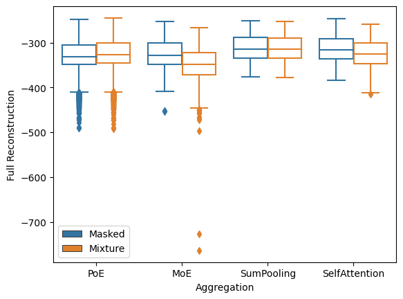
(a)

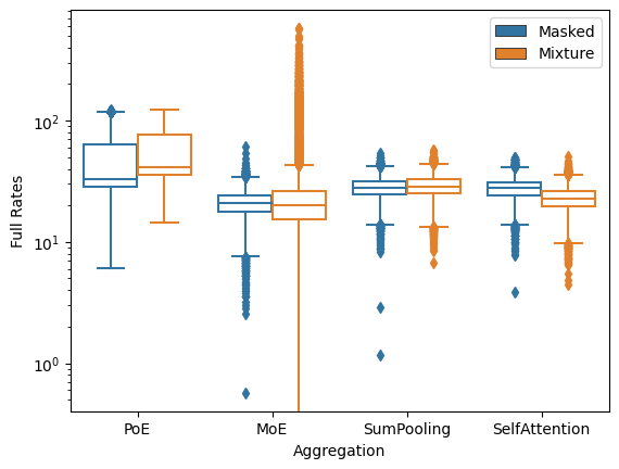
(b)

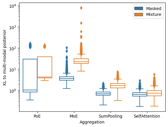
(c)

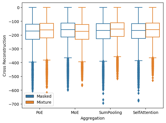
(d)

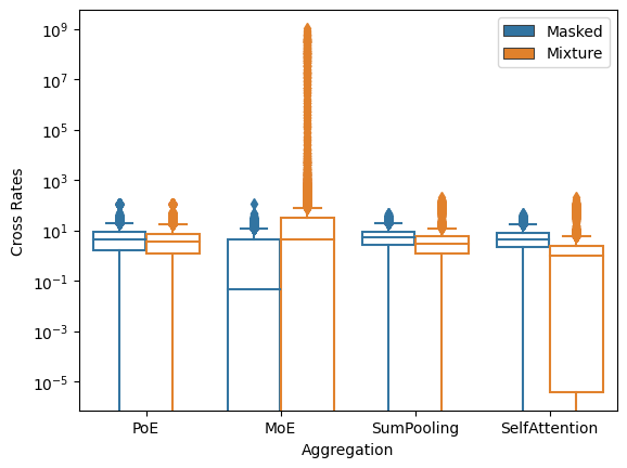
(e)

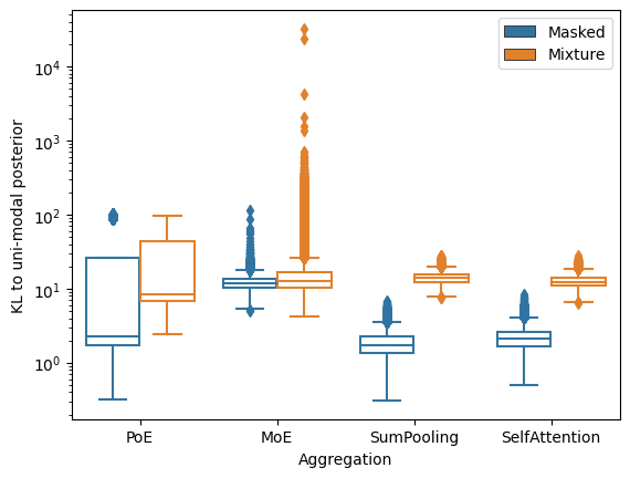
(f)

Figure 3: Linear Gaussian models with dense decoder matrix: Rate and distortion terms and KL-divergence of encoding distributions to posterior distribution from learned generative model.

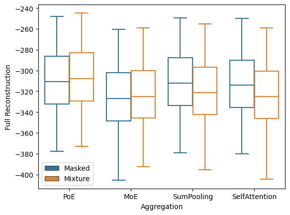
(a)

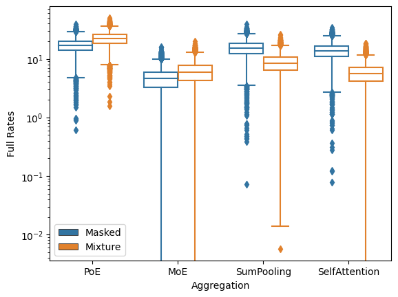
(b)

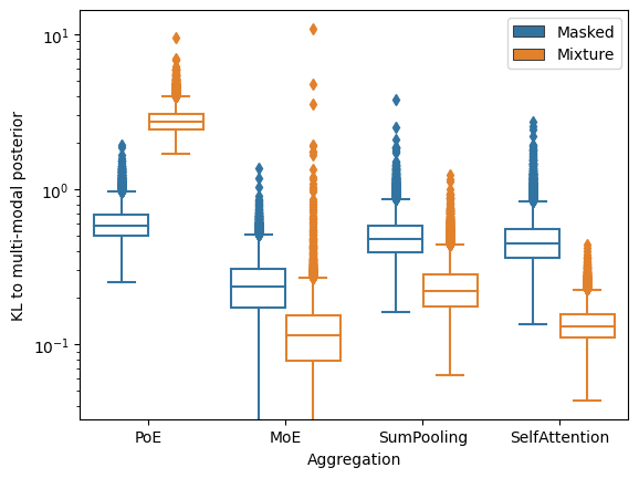
(c)

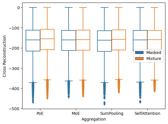
(d)

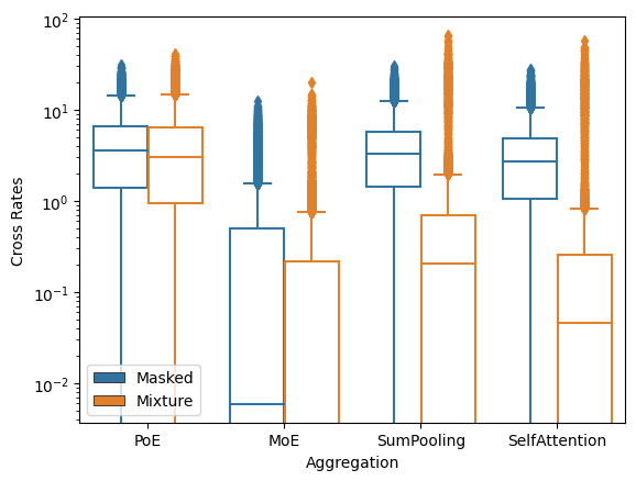
(e)

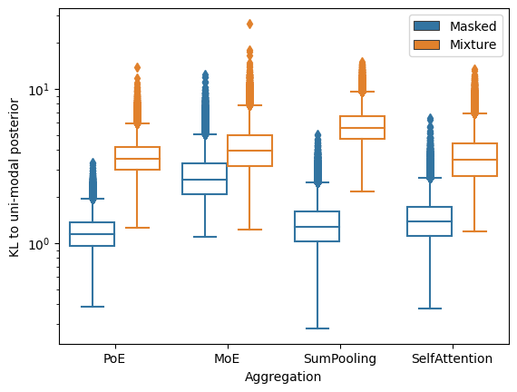
(f)

Figure 4: Linear Gaussian models with sparse decoder matrix: Rate and distortion terms and KL-divergence of encoding distributions to posterior distribution from learned generative model.

Table 5: Multi-modal Gaussian model with sparse decoders in the ground truth model: LLH Gap is the relative difference of the log-likelihood of the learned model relative to the log-likelihood based on the exact MLE. Bound gap is the relative difference of the variational bound to the log-likelihood based on the MLE.

	Our bound			Mixture bound
Aggregation	LLH Gap	Bound Gap	MCC	LLH Gap	Bound Gap	MCC
PoE	0.00 (0.000)	0.00 (0.000)	0.84 (0.004)	0.00 (0.007)	0.01 (0.001)	0.87 (0.004)
MoE	0.01 (0.001)	0.01 (0.001)	0.81 (0.001)	0.01 (0.002)	0.01 (0.002)	0.83 (0.003)
SumPooling	0.00 (0.000)	0.00 (0.000)	0.84 (0.015)	0.01 (0.001)	0.01 (0.002)	0.84 (0.013)
SelfAttention	0.00 (0.001)	0.00 (0.000)	0.84 (0.005)	0.01 (0.002)	0.01 (0.002)	0.83 (0.004)

Table 6: Multi-modal Gaussian model with sparse decoders in the ground truth model and permutation-equivariant encoders: LLH Gap is the relative difference of the log-likelihood of the learned model relative to the log-likelihood based on the exact MLE. Bound gap is the relative difference of the variational bound to the log-likelihood based on the MLE.

	Our bound			Mixture bound
Aggregation	LLH Gap	Bound Gap	MCC	LLH Gap	Bound Gap	MCC
PoE (equivariant)	0.00 (0.000)	0.00 (0.000)	0.91 (0.016)	0.01 (0.001)	0.02 (0.001)	0.88 (0.011)
SumPooling (equivariant)	0.00 (0.000)	0.00 (0.000)	0.85 (0.004)	0.00 (0.000)	0.00 (0.001)	0.82 (0.003)
SelfAttention (equivariant)	0.00 (0.000)	0.00 (0.000)	0.83 (0.006)	0.00 (0.000)	0.00 (0.003)	0.83 (0.003)

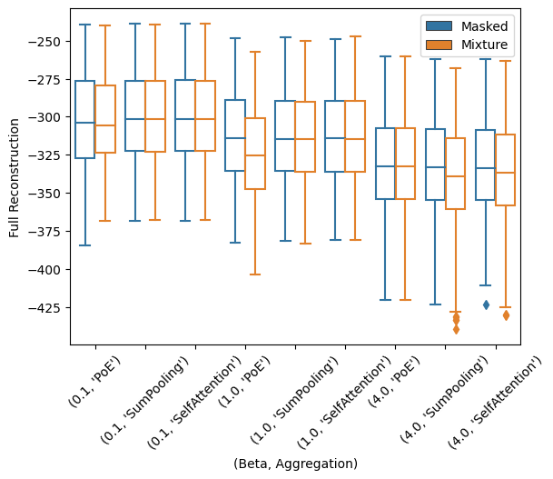
(a)

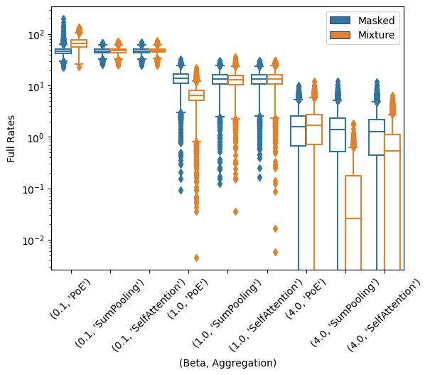
(b)

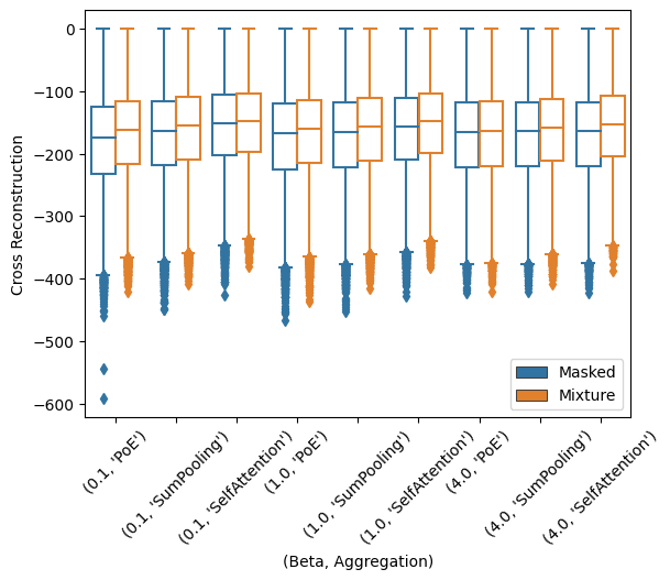
(c)

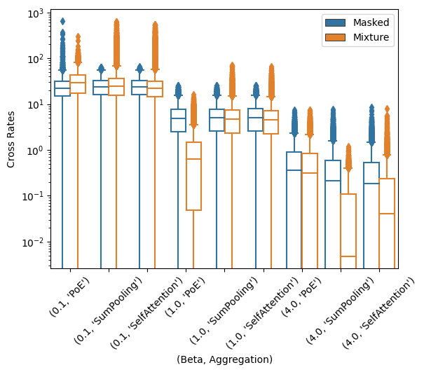
(d)

Figure 5: Linear Gaussian models with sparse decoder matrix and permutation-equivariant aggregation: Rate and distortion terms for varying $\beta$.

Appendix N Non-linear identifiable models

N.1 Auxiliary labels

Table 19 illustrates first the benefits of our bound that obtain better log-likelihood estimates for different fusion schemes. Second, it demonstrates the advantages of our new fusion schemes that achieve better log-likelihoods for both bounds. Third, it shows the benefit of using aggregation schemes that have the capacity to accommodate prior distributions different from a single Gaussian. Observe also that MoE schemes lead to low MCC values, while PoE schemes had high MCC values. We also show in Figure 6 the reconstructed modality values and inferred latent variables for one realisation with our bound, with the corresponding results for a mixture-based bound in Figure 7.

Table 7: Non-linear identifiable model with one real-valued modality and an auxiliary label acting as a second modality: The first four rows use a fixed standard Gaussian prior, while the last four rows use a Gaussian mixture prior with $5$ components. Mean and standard deviation over 4 repetitions.

	Our bound			Mixture bound
Aggregation	LLH ($\beta=1$)	MCC ($\beta=1$)	MCC ($\beta=0.1$)	LLH ($\beta=1$)	MCC ($\beta=1$)	MCC ($\beta=0.1$)
PoE	-43.4 (10.74)	0.98 (0.006)	0.99 (0.003)	-318 (361.2)	0.97 (0.012)	0.98 (0.007)
MoE	-20.5 (6.18)	0.94 (0.013)	0.93 (0.022)	-57.9 (6.23)	0.93 (0.017)	0.93 (0.025)
SumPooling	-17.9 (3.92)	0.99 (0.004)	0.99 (0.002)	-18.9 (4.09)	0.99 (0.005)	0.99 (0.008)
SelfAttention	-18.2 (4.17)	0.99 (0.004)	0.99 (0.003)	-18.6 (3.73)	0.99 (0.004)	0.99 (0.007)
SumPooling	-15.4 (2.12)	1.00 (0.001)	0.99 (0.004)	-18.6 (2.36)	0.98 (0.008)	0.99 (0.006)
SelfAttention	-15.2 (2.05)	1.00 (0.001)	1.00 (0.004)	-18.6 (2.27)	0.98 (0.014)	0.98 (0.006)
SumPoolingMixture	-15.1 (2.15)	1.00 (0.001)	0.99 (0.012)	-18.2 (2.80)	0.98 (0.010)	0.99 (0.005)
SelfAttentionMixture	-15.3 (2.35)	0.99 (0.005)	0.99 (0.004)	-18.4 (2.63)	0.99 (0.007)	0.99 (0.007)

N.2 Five continuous modalities

Table 8 demonstrates that our bound can yield to higher log-likelihoods and tigher bounds compared to a mixture-based bound, as do more flexible fusion schemes. Similar results for the partially observed case $(\eta=0.5)$ have been illustrated in the main text in Table 2.

Table 8: Fully observed ($\eta=0$) non-linear identifiable model with 5 modalities: The first four rows use a fixed standard Gaussian prior, while the last four rows use a Gaussian mixture prior with 5 components. Mean and standard deviation over 4 repetitions.

	Our bound			Mixture bound
Aggregation	LLH	Lower Bound	MCC	LLH	Lower Bound	MCC
PoE	-473.6 (9.04)	-476.9 (9.61)	0.98 (0.005)	-497.7 (11.26)	-559.0 (2.33)	0.97 (0.008)
MoE	-477.9 (8.50)	-484.3 (8.88)	0.91 (0.014)	-494.6 (9.20)	-546.8 (7.02)	0.92 (0.004)
SumPooling	-471.4 (8.29)	-472.3 (8.54)	0.99 (0.004)	-480.5 (8.84)	-530.5 (3.02)	0.98 (0.005)
SelfAttention	-471.4 (8.97)	-472.3 (9.52)	0.99 (0.002)	-482.8 (10.51)	-532.7 (2.89)	0.98 (0.004)
SumPooling	-465.4 (8.16)	-467.6 (8.25)	0.98 (0.002)	-475.1 (7.54)	-521.7 (3.55)	0.98 (0.003)
SelfAttention	-469.3 (4.76)	-471.5 (4.99)	0.98 (0.003)	-474.7 (8.20)	-522.7 (2.79)	0.98 (0.002)
SumPoolingMixture	-464.5 (8.16)	-466.3 (7.91)	0.99 (0.003)	-474.2 (7.61)	-521.2 (4.13)	0.98 (0.004)
SelfAttentionMixture	-464.4 (8.50)	-466.0 (9.66)	0.99 (0.003)	-473.6 (8.24)	-520.6 (2.62)	0.98 (0.002)

(a)

(b)

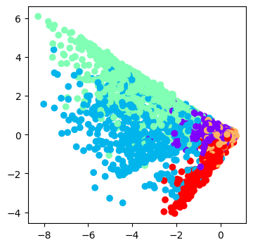
(c)

(d)

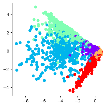
(e)

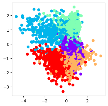
(f)

(g)

(h)

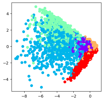
(i)

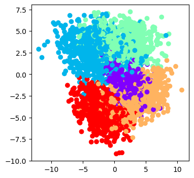
(j)

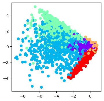
(k)

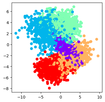
(l)

Figure 6: Bi-modal non-linear model with label and continuous modality based on our bound.

(a)

(b)

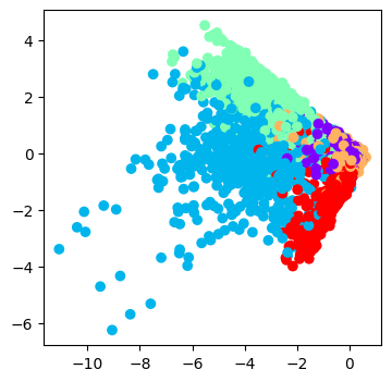
(c)

(d)

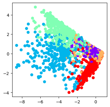
(e)

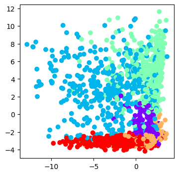
(f)

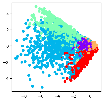
(g)

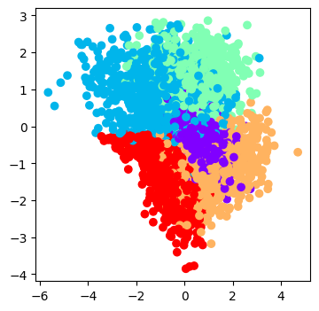
(h)

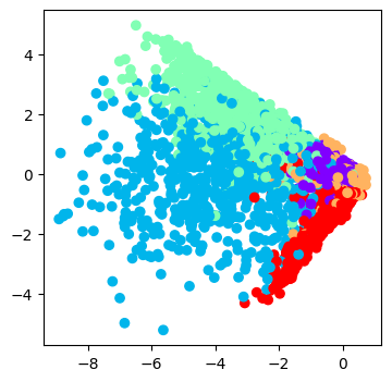
(i)

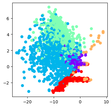
(j)

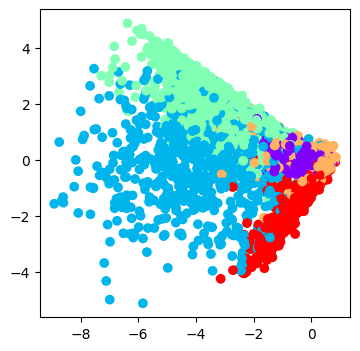
(k)

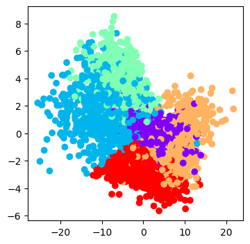
(l)

Figure 7: Bi-modal non-linear model with label and continuous modality based on mixture bound.

Appendix O MNIST-SVHN-Text

O.1 Training hyperparamters

The MNIST-SVHN-Text data set is taken from the code accompanying [115] with around 1.1 million train and 200k test samples. All models are trained for 100 epochs with a batch size of 250 using Adam [66] and a cosine decay schedule from 0.0005 to 0.0001.

O.2 Multi-modal rates and distortions

(a)

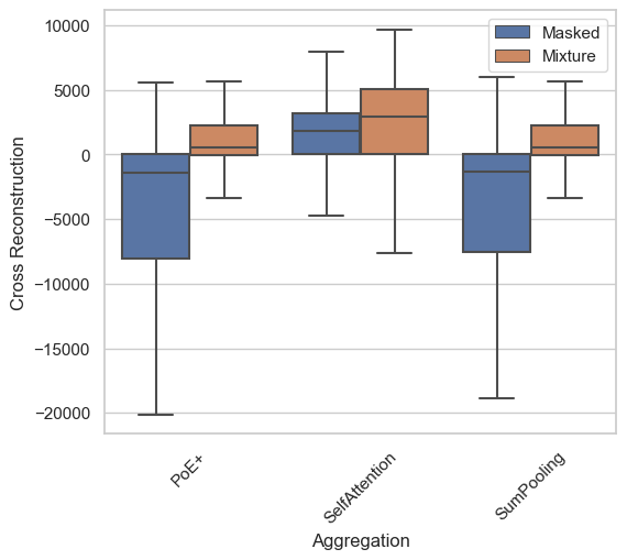
(b)

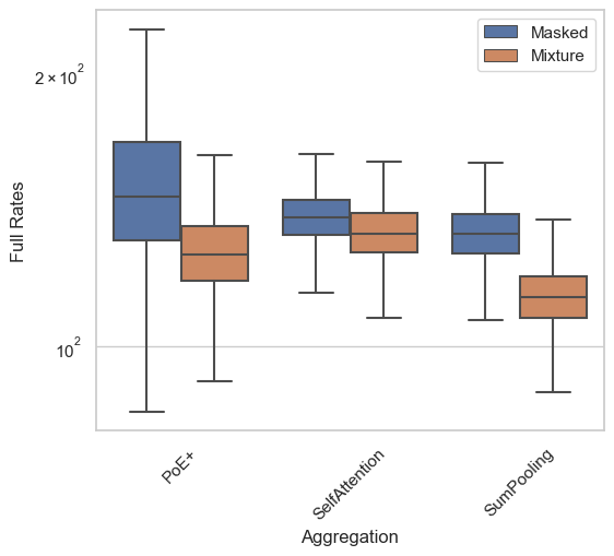
(c)

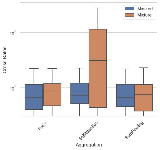
(d)

Figure 8: Rate and distortion terms for MNIST-SVHN-Text with shared and private latent variables.

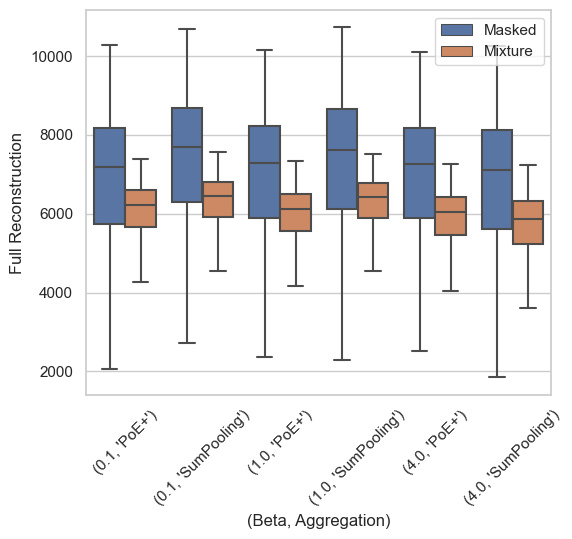
(a)

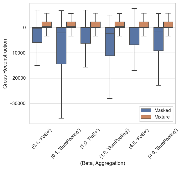
(b)

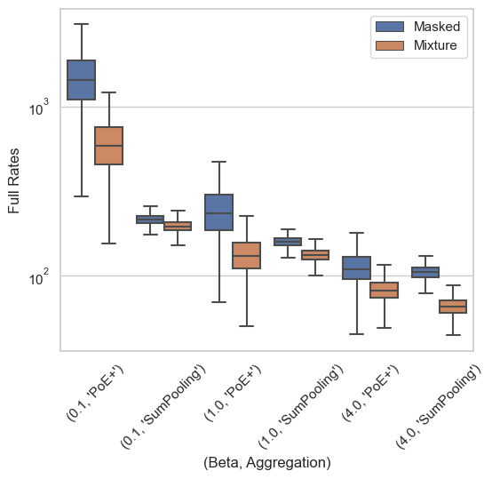
(c)

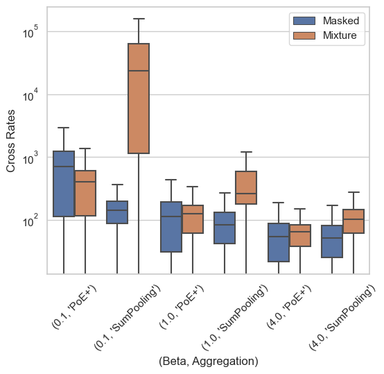
(d)

Figure 9: Rate and distortion terms for MNIST-SVHN-Text with shared latent variables and different $\beta$.

O.3 Log-likelihood estimates

Table 9: Test log-likelihood estimates for varying $\beta$ choices for the joint data (M+S+T) as well as for the marginal data of each modality based on importance sampling (512 particles). Multi-modal generative model with a $40$-dimensional shared latent variable.

	Our bound				Mixture bound
($\beta$, Aggregation)	M+S+T	M	S	T	M+S+T	M	S	T
(0.1, PoE+)	5433 (24.5)	1786 (41.6)	3578 (63.5)	-29 (2.4)	5481 (18.4)	2207 (19.8)	3180 (33.7)	-39 (1.0)
(0.1, SumPooling)	7067 (78.0)	2455 (3.3)	4701 (83.5)	-9 (0.4)	6061 (15.7)	2398 (9.3)	3552 (7.4)	-50 (1.9)
(1.0, PoE+)	6872 (9.6)	2599 (5.6)	4317 (1.1)	-9 (0.2)	5900 (10.0)	2449 (10.4)	3443 (11.7)	-19 (0.4)
(1.0, SumPooling)	7056 (124.4)	2478 (9.3)	4640 (113.9)	-6 (0.0)	6130 (4.4)	2470 (10.3)	3660 (1.5)	-16 (1.6)
(4.0, PoE+)	7021 (13.3)	2673 (13.2)	4413 (30.5)	-5 (0.1)	5895 (6.2)	2484 (5.5)	3434 (2.2)	-13 (0.4)
(4.0, SumPooling)	6690 (113.4)	2483 (9.9)	4259 (117.2)	-5 (0.0)	5659 (48.3)	2448 (10.5)	3233 (27.7)	-10 (0.2)

O.4 Generated modalities

O.5 Conditional coherence

Table 10: Conditional coherence for models with shared latent variables and bi-modal conditionals. The letters on the second line represent the modality which is generated based on the sets of modalities on the line below it.

Our bound									Mixture bound
	M			S			T			M			S			T
Aggregation	M+S	M+T	S+T	M+S	M+T	S+T	M+S	M+T	S+T	M+S	M+T	S+T	M+S	M+T	S+T	M+S	M+T	S+T
PoE	0.98	0.98	0.60	0.75	0.58	0.77	0.82	1.00	1.00	0.96	0.97	0.95	0.61	0.11	0.61	0.45	0.99	0.98
PoE+	0.97	0.98	0.55	0.73	0.52	0.75	0.83	1.00	0.99	0.97	0.97	0.96	0.64	0.11	0.63	0.45	0.99	0.97
MoE	0.88	0.97	0.90	0.35	0.11	0.35	0.41	0.72	0.69	0.88	0.96	0.89	0.32	0.10	0.33	0.42	0.72	0.69
MoE+	0.85	0.94	0.86	0.32	0.10	0.32	0.40	0.71	0.67	0.87	0.96	0.89	0.32	0.10	0.32	0.42	0.72	0.69
SumPooling	0.97	0.97	0.86	0.78	0.30	0.80	0.76	0.99	1.00	0.97	0.97	0.95	0.65	0.10	0.65	0.45	0.99	0.97
SelfAttention	0.97	0.97	0.82	0.76	0.30	0.78	0.69	1.00	1.00	0.97	0.97	0.99	0.66	0.10	0.65	0.45	0.99	1.00

Table 11: Conditional coherence for models with private latent variables and uni-modal conditionals. The letters on the second line represent the modality which is generated based on the sets of modalities on the line below it.

Our bound									Mixture bound
	M			S			T			M			S			T
Aggregation	M	S	T	M	S	T	M	S	T	M	S	T	M	S	T	M	S	T
PoE+	0.97	0.12	0.13	0.20	0.62	0.24	0.16	0.15	1.00	0.96	0.83	0.99	0.11	0.58	0.11	0.44	0.39	1.00
SumPooling	0.97	0.42	0.59	0.44	0.67	0.40	0.65	0.45	1.00	0.97	0.86	0.99	0.11	0.62	0.11	0.45	0.40	1.00
SelfAttention	0.97	0.12	0.12	0.27	0.71	0.28	0.46	0.40	1.00	0.96	0.09	0.08	0.12	0.67	0.12	0.15	0.17	1.00

Table 12: Conditional coherence for models with private latent variables and bi-modal conditionals. The letters on the second line represent the modality which is generated based on the sets of modalities on the line below it.

Our bound									Mixture bound
	M			S			T			M			S			T
Aggregation	M+S	M+T	S+T	M+S	M+T	S+T	M+S	M+T	S+T	M+S	M+T	S+T	M+S	M+T	S+T	M+S	M+T	S+T
PoE+	0.97	0.97	0.14	0.66	0.33	0.67	0.18	1.00	1.00	0.97	0.97	0.94	0.63	0.11	0.63	0.45	0.99	0.96
SumPooling	0.97	0.97	0.54	0.79	0.43	0.80	0.57	1.00	1.00	0.97	0.97	0.93	0.64	0.11	0.63	0.45	0.99	0.97
SelfAttention	0.97	0.97	0.12	0.80	0.29	0.81	0.49	1.00	1.00	0.96	0.96	0.08	0.70	0.12	0.70	0.15	1.00	1.00

Table 13: Conditional coherence for models with shared latent variables for different $\beta$s and uni-modal conditionals. The letters on the second line represent the modality which is generated based on the sets of modalities on the line below it.

Our bound									Mixture bound
	M			S			T			M			S			T
($\beta$, Aggregation)	M	S	T	M	S	T	M	S	T	M	S	T	M	S	T	M	S	T
(0.1, PoE+)	0.98	0.11	0.12	0.12	0.62	0.14	0.61	0.25	1.00	0.96	0.83	0.99	0.11	0.58	0.11	0.45	0.39	1.00
(0.1, SumPooling)	0.97	0.48	0.81	0.30	0.72	0.33	0.86	0.55	1.00	0.97	0.86	0.99	0.11	0.64	0.11	0.45	0.40	1.00
(1.0, PoE+)	0.97	0.15	0.63	0.24	0.63	0.42	0.79	0.35	1.00	0.96	0.83	0.99	0.11	0.59	0.11	0.45	0.39	1.00
(1.0, SumPooling)	0.97	0.48	0.87	0.25	0.72	0.36	0.73	0.48	1.00	0.97	0.86	0.99	0.10	0.63	0.10	0.45	0.40	1.00
(4.0, PoE+)	0.97	0.29	0.83	0.41	0.60	0.58	0.76	0.38	1.00	0.96	0.82	0.99	0.10	0.57	0.10	0.44	0.38	1.00
(4.0, SumPooling)	0.97	0.48	0.88	0.35	0.66	0.44	0.83	0.53	1.00	0.96	0.85	0.99	0.11	0.57	0.10	0.45	0.39	1.00

Table 14: Conditional coherence for models with shared latent variables for different $\beta$s and bi-modal conditionals. The letters on the second line represent the modality which is generated based on the sets of modalities on the line below it.

Our bound									Mixture bound
	M			S			T			M			S			T
($\beta$, Aggregation)	M+S	M+T	S+T	M+S	M+T	S+T	M+S	M+T	S+T	M+S	M+T	S+T	M+S	M+T	S+T	M+S	M+T	S+T
(0.1, PoE+)	0.98	0.98	0.15	0.70	0.14	0.72	0.66	1.00	1.00	0.96	0.96	0.93	0.62	0.11	0.62	0.45	0.99	0.95
(0.1, SumPooling)	0.97	0.97	0.86	0.83	0.31	0.84	0.85	0.99	1.00	0.97	0.97	0.94	0.66	0.11	0.65	0.45	0.99	0.96
(1.0, PoE+)	0.97	0.98	0.55	0.73	0.52	0.75	0.83	1.00	0.99	0.97	0.97	0.96	0.64	0.11	0.63	0.45	0.99	0.97
(1.0, SumPooling)	0.97	0.97	0.86	0.78	0.30	0.80	0.76	0.99	1.00	0.97	0.97	0.95	0.65	0.10	0.65	0.45	0.99	0.97
(4.0, PoE+)	0.97	0.98	0.84	0.76	0.66	0.78	0.82	1.00	1.00	0.97	0.97	0.96	0.62	0.10	0.62	0.45	0.99	0.98
(4.0, SumPooling)	0.97	0.97	0.89	0.77	0.40	0.78	0.86	0.99	1.00	0.97	0.97	0.96	0.61	0.10	0.60	0.45	0.99	0.97

Latent classification accuracy.

Table 15: Unsupervised latent classification for $\beta=1$ and models with shared latent variables only (top half) and shared plus private latent variables (bottom half). Accuracy is computed with a linear classifier (logistic regression) trained on multi-modal inputs (M+S+T) or uni-modal inputs (M, S or T).

	Our bound				Mixture bound
Aggregation	M+S+T	M	S	T	M+S+T	M	S	T
PoE	0.988 (0.000)	0.940 (0.009)	0.649 (0.039)	0.998 (0.001)	0.991 (0.004)	0.977 (0.002)	0.845 (0.000)	1.000 (0.000)
PoE+	0.978 (0.002)	0.934 (0.001)	0.624 (0.040)	0.999 (0.001)	0.998 (0.000)	0.981 (0.000)	0.851 (0.000)	1.000 (0.000)
MoE	0.841 (0.008)	0.974 (0.000)	0.609 (0.032)	1.000 (0.000)	0.940 (0.001)	0.980 (0.001)	0.843 (0.001)	1.000 (0.000)
MoE+	0.850 (0.039)	0.967 (0.014)	0.708 (0.167)	0.983 (0.023)	0.928 (0.017)	0.983 (0.002)	0.846 (0.001)	1.000 (0.000)
SelfAttention	0.985 (0.001)	0.954 (0.002)	0.693 (0.037)	0.986 (0.006)	0.991 (0.000)	0.981 (0.001)	0.864 (0.003)	1.000 (0.000)
SumPooling	0.981 (0.000)	0.962 (0.000)	0.704 (0.014)	0.992 (0.008)	0.994 (0.000)	0.983 (0.000)	0.866 (0.002)	1.000 (0.000)
PoE+	0.979 (0.009)	0.944 (0.000)	0.538 (0.032)	0.887 (0.07)	0.995 (0.002)	0.980 (0.002)	0.848 (0.006)	1.000 (0.000)
SumPooling	0.987 (0.004)	0.966 (0.004)	0.370 (0.348)	0.992 (0.002)	0.994 (0.001)	0.982 (0.000)	0.870 (0.001)	1.000 (0.000)
SelfAttention	0.990 (0.003)	0.968 (0.002)	0.744 (0.008)	0.985 (0.000)	0.997 (0.001)	0.974 (0.000)	0.681 (0.031)	1.000 (0.000)

Table 16: Unsupervised latent classification for different $\beta$s and models with shared latent variables only. Accuracy is computed with a linear classifier (logistic regression) trained on multi-modal inputs (M+S+T) or uni-modal inputs (M, S or T).

	Our bound				Mixture bound
($\beta$, Aggregation)	M+S+T	M	S	T	M+S+T	M	S	T
(0.1, PoE+)	0.983 (0.006)	0.919 (0.001)	0.561 (0.048)	0.988 (0.014)	0.992 (0.002)	0.979 (0.002)	0.846 (0.004)	1.000 (0.000)
(0.1, SumPooling)	0.982 (0.004)	0.965 (0.002)	0.692 (0.047)	0.999 (0.001)	0.994 (0.000)	0.981 (0.002)	0.863 (0.005)	1.000 (0.000)
(1.0, PoE+)	0.978 (0.002)	0.934 (0.001)	0.624 (0.040)	0.999 (0.001)	0.998 (0.000)	0.981 (0.000)	0.851 (0.000)	1.000 (0.000)
(1.0, SumPooling)	0.981 (0.000)	0.962 (0.000)	0.704 (0.014)	0.992 (0.008)	0.994 (0.000)	0.983 (0.000)	0.866 (0.002)	1.000 (0.000)
(4.0, PoE+)	0.981 (0.006)	0.943 (0.007)	0.630 (0.008)	0.993 (0.001)	0.998 (0.000)	0.981 (0.000)	0.846 (0.001)	1.000 (0.000)
(4.0, SumPooling)	0.984 (0.004)	0.963 (0.001)	0.681 (0.009)	0.995 (0.000)	0.992 (0.002)	0.980 (0.001)	0.856 (0.001)	1.000 (0.000)

Appendix P Encoder Model architectures

P.1 Linear models

Table 17: Encoder architectures for Gaussian models.

(a) Modality-specific encoding functions $h_{s}(x_{s})$. Latent dimension $D=30$, modality dimension $D_{s}\sim\mathcal{U}(30,60)$.

MoE/PoE	SumPooling/SelfAttention
Input: $D_{s}$	Input: $D_{s}$
Dense $D_{s}\times 512$, ReLU	Dense $D_{s}\times 256$, ReLU
Dense $512\times 512$, ReLU	Dense $256\times 256$, ReLU
Dense $512\times 60$	Dense $256\times 60$

(b) Model for outer aggregation function $\rho_{\vartheta}$ for SumPooling and SelfAttention schemes.

Outer Aggregation
Input: $256$
Dense $256\times 256$, ReLU
Dense $256\times 256$, ReLU
Dense $256\times 60$

(c) Inner aggregation function $\chi_{\vartheta}$.

SumPooling	SelfAttention
Input: $256$	Input: $256$
Dense $256\times 256$, ReLU	Dense $256\times 256$, ReLU
Dense $256\times 256$, ReLU	Dense $256\times 256$
Dense $256\times 256$

(d) Transformer parameters.

SelfAttention (1 Layer)
Input: $256$
Heads: $4$
Attention size: $256$
Hidden size FFN: $256$

P.2 Linear models with private latent variables

Table 18: Encoder architectures for Gaussian models with private latent variables.

(a) Modality-specific encoding functions $h_{s}(x_{s})$. All private and shared latent variables are of dimension $10$. Modality dimension $D_{s}\sim\mathcal{U}(30,60)$.

PoE ($h_{s}^{\text{shared}}$ and $h_{s}^{\text{private}}$)	SumPooling/SelfAttention (one $h_{s}$)
Input: $D_{s}$	Input: $D_{s}$
Dense $D_{s}\times 512$, ReLU	Dense $D_{s}\times 128$, ReLU
Dense $512\times 512$, ReLU	Dense $128\times 128$, ReLU
Dense $512\times 10$	Dense $128\times 10$

(b) Model for outer aggregation function $\rho_{\vartheta}$ for SumPooling scheme.

Outer Aggregation ($\rho_{\vartheta}$)
Input: $128$
Dense $128\times 128$, ReLU
Dense $128\times 128$, ReLU
Dense $128\times 10$

(c) Inner aggregation functions.

SumPooling ($\chi_{0,\vartheta}$, $\chi_{1,\vartheta}$, $\chi_{2,\vartheta}$)	SelfAttention $(\chi_{1,\vartheta}$, $\chi_{2,\vartheta}$)
Input: $128$	Input: $128$
Dense $128\times 128$, ReLU	Dense $128\times 128$, ReLU
Dense $128\times 128$, ReLU	Dense $128\times 128$
Dense $128\times 128$

(d) Transformer parameters.

SelfAttention (1 Layer)
Input: $128$
Heads: $4$
Attention size: $128$
Hidden size FFN: $128$

P.3 Nonlinear model with auxiliary label

Table 19: Encoder architectures for nonlinear model with auxiliary label.

(a) Modality-specific encoding functions $h_{s}(x_{s})$. Modality dimension $D_{1}=2$ (continuous modality) and $D_{2}=5$ (label). Embedding dimension $D_{E}=4$ for PoE and MoE and $D_{E}=128$ otherwise.

Modality-specific encoders
Input: $D_{s}$
Dense $D_{s}\times 128$, ReLU
Dense $128\times 128$, ReLU
Dense $128\times D_{E}$

(b) Model for outer aggregation function $\rho_{\vartheta}$ for SumPooling and SelfAttention schemes and mixtures thereof. Output dimension is $D_{0}=25$ for mixture densities and $D_{O}=4$ otherwise.

Outer Aggregation
Input: $128$
Dense $128\times 128$, ReLU
Dense $128\times 128$, ReLU
Dense $128\times D_{O}$

(c) Inner aggregation function $\chi_{\vartheta}$.

SumPooling	SelfAttention
Input: $128$	Input: $128$
Dense $128\times 128$, ReLU	Dense $128\times 128$, ReLU
Dense $128\times 128$, ReLU	Dense $128\times 128$
Dense $128\times 128$

(d) Transformer parameters.

SelfAttention
Input: $128$
Heads: $4$
Attention size: $128$
Hidden size FFN: $128$

P.4 Nonlinear model with five modalities

Table 20: Encoder architectures for nonlinear model with five modalities.

(a) Modality-specific encoding functions $h_{s}(x_{s})$. Modality dimensions $D_{s}=25$. Latent dimension $D=25$

MoE/PoE	SumPooling/SelfAttention
Input: $D_{s}$	Input: $D_{s}$
Dense $D_{s}\times 512$, ReLU	Dense $D_{s}\times 256$, ReLU
Dense $512\times 512$, ReLU	Dense $256\times 256$, ReLU
Dense $512\times 50$	Dense $256\times 256$

(b) Model for outer aggregation function $\rho_{\vartheta}$ for SumPooling and SelfAttention schemes and mixtures thereof. Output dimension is $D_{0}=50$ for mixture densities and $D_{O}=25$ otherwise.

Outer Aggregation
Input: $256$
Dense $256\times 256$, ReLU
Dense $256\times 256$, ReLU
Dense $256\times D_{O}$

(c) Inner aggregation function $\chi_{\vartheta}$.

SumPooling	SelfAttention
Input: $256$	Input: $256$
Dense $256\times 256$, ReLU	Dense $256\times 256$, ReLU
Dense $256\times 256$, ReLU	Dense $\times 256$
Dense $256\times 256$

(d) Transformer parameters.

SelfAttention
Input: $256$
Heads: $4$
Attention size: $256$
Hidden size FFN: $256$

P.5 MNIST-SVHN-Text

For SVHN and and Text, we use 2d- or 1d-convolutional layers, respectively, denoted as Conv($f,k,s$) for feature dimension $f$, kernel-size $k$ and stride $s$. We denote transposed convolutions as tConv. We use the neural network architectures as implemented in Flax [44].

Table 21: Encoder architectures for MNIST-SVHN-Text.

(a) MNIST-specific encoding functions $h_{s}(x_{s})$. Modality dimensions $D_{s}=28\times 28$. Embedding dimension is $D_{E}=2D$ for PoE/MoE and $D_{E}=256$ for SumPooling/SelfAttention. For PoE+/MoE+, we add four times a Dense layer of size $256$ with ReLU layer before the last linear layer.

MoE/PoE/SumPooling/SelfAttention
Input: $D_{s}$,
Dense $D_{s}\times 400$, ReLU
Dense $400\times 400$, ReLU
Dense $400\times D_{E}$

(b) SVHN-specific encoding functions $h_{s}(x_{s})$. Modality dimensions $D_{s}=3\times 32\times 32$. Embedding dimension is $D_{E}=2D$ for PoE/MoE and $D_{E}=256$ for SumPooling/SelfAttention. For PoE+/MoE+, we add four times a Dense layer of size $256$ with ReLU layer before the last linear layer.

MoE/PoE/SumPooling/SelfAttention
Input: $D_{s}$
Conv(32, 4, 2), ReLU
Conv(64, 4, 2), ReLU
Conv(64, 4, 2), ReLU
Conv(128, 4, 2), ReLU, Flatten
Dense $2048\times D_{E}$

(c) Text-specific encoding functions $h_{s}(x_{s})$. Modality dimensions $D_{s}=8\times 71$. Embedding dimension is $D_{E}=2D$ for PoE/MoE and $D_{E}=256$ for permutation-invariant models (SumPooling/SelfAttention) and $D_{E}=128$ for permutation-equivariant models (SumPooling/SelfAttention). For PoE+/MoE+, we add four times a Dense layer of size $256$ with ReLU layer before the last linear layer.

MoE/PoE/SumPooling/SelfAttention
Input: $D_{s}$
Conv(128, 1, 1), ReLU
Conv(128, 4, 2), ReLU
Conv(128, 4, 2), ReLU, Flatten
Dense $128\times D_{E}$

(d) Model for outer aggregation function $\rho_{\vartheta}$ for SumPooling and SelfAttention schemes. Output dimension is $D_{0}=2D=80$ for models with shared latent variables only and $D_{0}=10+10$ for models with private and shared latent variables. $D_{E}=256$ for permutation-invariant and $D_{I}=128$ for permutation-invariant models.

Outer Aggregation
Input: $D_{E}$
Dense $D_{E}\times D_{E}$, LReLU
Dense $D_{E}\times D_{E}$, LReLU
Dense $D_{E}\times D_{O}$

(e) Inner aggregation function $\chi_{\vartheta}$ for permutation-invariant models ($D_{E}=256$) and permutaion-equivariant models ($D_{E}=128$).

SumPooling	SelfAttention
Input: $D_{E}$	Input: $D_{E}$
Dense $D_{E}\times D_{E}$, LReLU	Dense $D_{E}\times D_{E}$, LReLU
Dense $D_{E}\times D_{E}$, LReLU	Dense $\times D_{E}$
Dense $D_{E}\times D_{E}$

(f) Transformer parameters for permutation-invariant models. $D_{E}=256$ for permutation-invariant and $D_{I}=128$ for permutation-invariant models.

SelfAttention ($2$ Layers)
Input: $D_{E}$
Heads: $4$
Attention size: $D_{E}$
Hidden size FFN: $D_{E}$

P.6 MNIST-SVHN-Text with private latent variables

Appendix Q MNIST-SVHN-Text Decoder Model architectures

For models with private latent variables, we concatenate the shared and private latent variables. We use a Laplace likelihood as the decoding distribution for MNIST and SVHN, where the decoder function learns both its mean as a function of the latent and a constant log-standard-deviation at each pixel. Following previous works [110, 115], we re-weight the log-likelihoods for different modalities relative to their dimensions.

Table 22: Decoder architectures for MNIST-SVHN-Text.

(a) MNIST decoder. $D_{I}=40$ for models with shared latent variables only, and $D_{I}=10+10$ otherwise.

MNIST
Input: $D_{I}$
Dense $40\times 400$, ReLU
Dense $400\times 400$, ReLU
Dense $400\times D_{s}$, Sigmoid

(b) SVHN decoder. $D_{I}=40$ for models with shared latent variables only, and $D_{I}=10+10$ otherwise.

SVHN
Input: $D_{I}$
Dense $D_{I}\times 128$, ReLU
tConv(64, 4, 3), ReLU
tConv(64, 4, 2), ReLU
tConv(32, 4, 2), ReLU
tConv(3, 4, 2)

(c) Text decoder. $D_{I}=40$ for models with shared latent variables only, and $D_{I}=10+10$ otherwise.

Text
Input: $D_{I}$
Dense $D_{I}\times 128$, ReLU
tConv(128, 4, 3), ReLU
tConv(128, 4, 2), ReLU
tConv(71, 1, 1)

Appendix R Compute resources and existing assets

Our computations were performed on shared HPC systems. All experiments except Section 5.3 were run on a CPU server using one or two CPU cores. The experiments in Section 5.3 were run a GPU server using one NVIDIA A100.

Our implementation is based on JAX [16] and Flax [44]. We compute the mean correlation co-efficient (MCC) between true and infered latent variables following [63], as in https://github.com/ilkhem/icebeem. In our MNIST-SVHN-Text experiments, we use code from [115], https://github.com/thomassutter/MoPoE.

References

- Abbas [2009] A. E. Abbas. A Kullback-Leibler view of linear and log-linear pools. Decision Analysis, 6(1):25–37, 2009.
- Akaho [2001] S. Akaho. A kernel method for canonical correlation analysis. In International Meeting of Psychometric Society, 2001, 2001.
- Alemi et al. [2018] A. Alemi, B. Poole, I. Fischer, J. Dillon, R. A. Saurous, and K. Murphy. Fixing a broken elbo. In International conference on machine learning, pages 159–168. PMLR, 2018.
- Alemi et al. [2016] A. A. Alemi, I. Fischer, J. V. Dillon, and K. Murphy. Deep Variational Information Bottleneck. arXiv preprint arXiv:1612.00410, 2016.
- Allman et al. [2009] E. S. Allman, C. Matias, and J. A. Rhodes. Identifiability of parameters in latent structure models with many observed variables. The Annals of Statistics, 37(6A):3099–3132, 2009.
- Archambeau and Bach [2008] C. Archambeau and F. Bach. Sparse probabilistic projections. Advances in neural information processing systems, 21, 2008.
- Argelaguet et al. [2018] R. Argelaguet, B. Velten, D. Arnol, S. Dietrich, T. Zenz, J. C. Marioni, F. Buettner, W. Huber, and O. Stegle. Multi-Omics Factor Analysis—a framework for unsupervised integration of multi-omics data sets. Molecular systems biology, 14(6):e8124, 2018.
- Ba et al. [2016] J. L. Ba, J. R. Kiros, and G. E. Hinton. Layer normalization. arXiv preprint arXiv:1607.06450, 2016.
- Bach and Jordan [2005] F. R. Bach and M. I. Jordan. A Probabilistic Interpretation of Canonical Correlation Analysis. 2005.
- Bahdanau et al. [2014] D. Bahdanau, K. Cho, and Y. Bengio. Neural machine translation by jointly learning to align and translate. arXiv preprint arXiv:1409.0473, 2014.
- Barber and Agakov [2004] D. Barber and F. Agakov. The IM Algorithm: a variational approach to Information Maximization. Advances in neural information processing systems, 16(320):201, 2004.
- Bartunov et al. [2022] S. Bartunov, F. B. Fuchs, and T. P. Lillicrap. Equilibrium aggregation: Encoding sets via optimization. In Uncertainty in Artificial Intelligence, pages 139–149. PMLR, 2022.
- Biloš and Günnemann [2021] M. Biloš and S. Günnemann. Scalable normalizing flows for permutation invariant densities. In International Conference on Machine Learning, pages 957–967. PMLR, 2021.
- Blei et al. [2017] D. M. Blei, A. Kucukelbir, and J. D. McAuliffe. Variational inference: A review for statisticians. Journal of the American Statistical Association, 112(518):859–877, 2017.
- Bloem-Reddy and Teh [2020] B. Bloem-Reddy and Y. W. Teh. Probabilistic symmetries and invariant neural networks. J. Mach. Learn. Res., 21:90–1, 2020.
- Bradbury et al. [2018] J. Bradbury, R. Frostig, P. Hawkins, M. J. Johnson, C. Leary, D. Maclaurin, G. Necula, A. Paszke, J. VanderPlas, S. Wanderman-Milne, and Q. Zhang. JAX: composable transformations of Python+NumPy programs, 2018. URL http://github.com/google/jax.
- Browne [1980] M. Browne. Factor analysis of multiple batteries by maximum likelihood. British Journal of Mathematical and Statistical Psychology, 1980.
- Bruno et al. [2021] A. Bruno, J. Willette, J. Lee, and S. J. Hwang. Mini-batch consistent slot set encoder for scalable set encoding. Advances in Neural Information Processing Systems, 34:21365–21374, 2021.
- Chen et al. [2018] Z. Chen, V. Badrinarayanan, C.-Y. Lee, and A. Rabinovich. Gradnorm: Gradient normalization for adaptive loss balancing in deep multitask networks. In International conference on machine learning, pages 794–803. PMLR, 2018.
- Chung et al. [2015] J. Chung, K. Kastner, L. Dinh, K. Goel, A. C. Courville, and Y. Bengio. A recurrent latent variable model for sequential data. In Advances in neural information processing systems, pages 2980–2988, 2015.
- Dai et al. [2018] B. Dai, Y. Wang, J. Aston, G. Hua, and D. Wipf. Connections with robust PCA and the role of emergent sparsity in variational autoencoder models. The Journal of Machine Learning Research, 19(1):1573–1614, 2018.
- Daunhawer et al. [2022] I. Daunhawer, T. M. Sutter, K. Chin-Cheong, E. Palumbo, and J. E. Vogt. On the Limitations of Multimodal VAEs. In International Conference on Learning Representations, 2022.
- Daunhawer et al. [2023] I. Daunhawer, A. Bizeul, E. Palumbo, A. Marx, and J. E. Vogt. Identifiability results for multimodal contrastive learning. arXiv preprint arXiv:2303.09166, 2023.
- Dhariwal and Nichol [2021] P. Dhariwal and A. Nichol. Diffusion models beat GANs on image synthesis. Advances in Neural Information Processing Systems, 34:8780–8794, 2021.
- Diaconis and Freedman [1980] P. Diaconis and D. Freedman. Finite exchangeable sequences. The Annals of Probability, pages 745–764, 1980.
- Dilokthanakul et al. [2016] N. Dilokthanakul, P. A. Mediano, M. Garnelo, M. C. Lee, H. Salimbeni, K. Arulkumaran, and M. Shanahan. Deep unsupervised clustering with Gaussian Mixture Variational Autoencoders. arXiv preprint arXiv:1611.02648, 2016.
- Edwards and Storkey [2016] H. Edwards and A. Storkey. Towards a neural statistician. arXiv preprint arXiv:1606.02185, 2016.
- Falck et al. [2021] F. Falck, H. Zhang, M. Willetts, G. Nicholson, C. Yau, and C. C. Holmes. Multi-facet clustering Variational Autoencoders. Advances in Neural Information Processing Systems, 34:8676–8690, 2021.
- Figurnov et al. [2018] M. Figurnov, S. Mohamed, and A. Mnih. Implicit reparameterization gradients. In Advances in Neural Information Processing Systems, pages 441–452, 2018.
- Fliege and Svaiter [2000] J. Fliege and B. F. Svaiter. Steepest descent methods for multicriteria optimization. Mathematical methods of operations research, 51:479–494, 2000.
- Foong et al. [2020] A. Foong, W. Bruinsma, J. Gordon, Y. Dubois, J. Requeima, and R. Turner. Meta-learning stationary stochastic process prediction with convolutional neural processes. Advances in Neural Information Processing Systems, 33:8284–8295, 2020.
- Gao et al. [2019] S. Gao, R. Brekelmans, G. Ver Steeg, and A. Galstyan. Auto-encoding total correlation explanation. In The 22nd International Conference on Artificial Intelligence and Statistics, pages 1157–1166. PMLR, 2019.
- Garnelo et al. [2018a] M. Garnelo, D. Rosenbaum, C. Maddison, T. Ramalho, D. Saxton, M. Shanahan, Y. W. Teh, D. Rezende, and S. A. Eslami. Conditional neural processes. In International conference on machine learning, pages 1704–1713. PMLR, 2018a.
- Garnelo et al. [2018b] M. Garnelo, J. Schwarz, D. Rosenbaum, F. Viola, D. J. Rezende, S. Eslami, and Y. W. Teh. Neural processes. arXiv preprint arXiv:1807.01622, 2018b.
- Genest and Zidek [1986] C. Genest and J. V. Zidek. Combining probability distributions: A critique and an annotated bibliography. Statistical Science, 1(1):114–135, 1986.
- Genest et al. [1986] C. Genest, K. J. McConway, and M. J. Schervish. Characterization of externally Bayesian pooling operators. The Annals of Statistics, pages 487–501, 1986.
- Ghalebikesabi et al. [2021] S. Ghalebikesabi, R. Cornish, L. J. Kelly, and C. Holmes. Deep generative pattern-set mixture models for nonignorable missingness. arXiv preprint arXiv:2103.03532, 2021.
- Giannone and Winther [2022] G. Giannone and O. Winther. Scha-vae: Hierarchical context aggregation for few-shot generation. In International Conference on Machine Learning, pages 7550–7569. PMLR, 2022.
- Gong et al. [2021] Y. Gong, H. Hajimirsadeghi, J. He, T. Durand, and G. Mori. Variational selective autoencoder: Learning from partially-observed heterogeneous data. In International Conference on Artificial Intelligence and Statistics, pages 2377–2385. PMLR, 2021.
- Hälvä and Hyvarinen [2020] H. Hälvä and A. Hyvarinen. Hidden markov nonlinear ica: Unsupervised learning from nonstationary time series. In Conference on Uncertainty in Artificial Intelligence, pages 939–948. PMLR, 2020.
- Hälvä et al. [2021] H. Hälvä, S. Le Corff, L. Lehéricy, J. So, Y. Zhu, E. Gassiat, and A. Hyvarinen. Disentangling identifiable features from noisy data with structured nonlinear ICA. Advances in Neural Information Processing Systems, 34:1624–1633, 2021.
- Hardoon et al. [2004] D. R. Hardoon, S. Szedmak, and J. Shawe-Taylor. Canonical correlation analysis: An overview with application to learning methods. Neural computation, 16(12):2639–2664, 2004.
- He et al. [2016] K. He, X. Zhang, S. Ren, and J. Sun. Identity mappings in deep residual networks. In Computer Vision–ECCV 2016: 14th European Conference, Amsterdam, The Netherlands, October 11–14, 2016, Proceedings, Part IV 14, pages 630–645. Springer, 2016.
- Heek et al. [2023] J. Heek, A. Levskaya, A. Oliver, M. Ritter, B. Rondepierre, A. Steiner, and M. van Zee. Flax: A neural network library and ecosystem for JAX, 2023. URL http://github.com/google/flax.
- Hewitt et al. [2018] L. B. Hewitt, M. I. Nye, A. Gane, T. Jaakkola, and J. B. Tenenbaum. The variational homoencoder: Learning to learn high capacity generative models from few examples. arXiv preprint arXiv:1807.08919, 2018.
- Higgins et al. [2017] I. Higgins, L. Matthey, A. Pal, C. Burgess, X. Glorot, M. Botvinick, S. Mohamed, and A. Lerchner. -VAE: Learning basic visual concepts with a constrained variational framework. In International conference on learning representations, 2017.
- Ho and Salimans [2022] J. Ho and T. Salimans. Classifier-free diffusion guidance. arXiv preprint arXiv:2207.12598, 2022.
- Hoffman and Johnson [2016] M. D. Hoffman and M. J. Johnson. ELBO surgery: yet another way to carve up the variational evidence lower bound. In Workshop in Advances in Approximate Bayesian Inference, NIPS, 2016.
- Hotelling [1936] H. Hotelling. Relations between two sets of variates. Biometrika, 28(3/4):321–377, 1936.
- Huang et al. [2020] S. Huang, A. Makhzani, Y. Cao, and R. Grosse. Evaluating lossy compression rates of deep generative models. arXiv preprint arXiv:2008.06653, 2020.
- Huang et al. [2022] Y. Huang, J. Lin, C. Zhou, H. Yang, and L. Huang. Modality competition: What makes joint training of multi-modal network fail in deep learning?(provably). arXiv preprint arXiv:2203.12221, 2022.
- Hwang et al. [2021] H. Hwang, G.-H. Kim, S. Hong, and K.-E. Kim. Multi-view representation learning via total correlation objective. Advances in Neural Information Processing Systems, 34:12194–12207, 2021.
- Hyvarinen and Morioka [2016] A. Hyvarinen and H. Morioka. Unsupervised feature extraction by time-contrastive learning and nonlinear ICA. Advances in neural information processing systems, 29, 2016.
- Hyvärinen and Pajunen [1999] A. Hyvärinen and P. Pajunen. Nonlinear Independent Component Analysis: Existence and uniqueness results. Neural networks, 12(3):429–439, 1999.
- Ipsen et al. [2021] N. B. Ipsen, P.-A. Mattei, and J. Frellsen. not-MIWAE: Deep Generative Modelling with Missing not at Random Data. In ICLR 2021-International Conference on Learning Representations, 2021.
- Javaloy et al. [2022] A. Javaloy, M. Meghdadi, and I. Valera. Mitigating Modality Collapse in Multimodal VAEs via Impartial Optimization. arXiv preprint arXiv:2206.04496, 2022.
- Jiang et al. [2017] Z. Jiang, Y. Zheng, H. Tan, B. Tang, and H. Zhou. Variational deep embedding: an unsupervised and generative approach to clustering. In Proceedings of the 26th International Joint Conference on Artificial Intelligence, pages 1965–1972, 2017.
- Johnson et al. [2016] M. J. Johnson, D. Duvenaud, A. B. Wiltschko, S. R. Datta, and R. P. Adams. Structured vaes: Composing probabilistic graphical models and variational autoencoders. arXiv preprint arXiv:1603.06277, 2016.
- Jordan et al. [1999] M. I. Jordan, Z. Ghahramani, T. S. Jaakkola, and L. K. Saul. An introduction to variational methods for graphical models. Machine learning, 37(2):183–233, 1999.
- Joy et al. [2021] T. Joy, Y. Shi, P. H. Torr, T. Rainforth, S. M. Schmon, and N. Siddharth. Learning multimodal VAEs through mutual supervision. arXiv preprint arXiv:2106.12570, 2021.
- Karami and Schuurmans [2021] M. Karami and D. Schuurmans. Deep probabilistic canonical correlation analysis. In Proceedings of the AAAI Conference on Artificial Intelligence, volume 35, pages 8055–8063, 2021.
- Khemakhem et al. [2020a] I. Khemakhem, D. Kingma, R. Monti, and A. Hyvarinen. Variational Autoencoders and nonlinear ICA: A unifying framework. In International Conference on Artificial Intelligence and Statistics, pages 2207–2217. PMLR, 2020a.
- Khemakhem et al. [2020b] I. Khemakhem, R. Monti, D. Kingma, and A. Hyvarinen. ICE-BeeM: Identifiable Conditional Energy-Based Deep Models Based on Nonlinear ICA. Advances in Neural Information Processing Systems, 33:12768–12778, 2020b.
- Kim et al. [2018] H. Kim, A. Mnih, J. Schwarz, M. Garnelo, A. Eslami, D. Rosenbaum, O. Vinyals, and Y. W. Teh. Attentive neural processes. In International Conference on Learning Representations, 2018.
- Kim et al. [2021] J. Kim, J. Yoo, J. Lee, and S. Hong. Setvae: Learning hierarchical composition for generative modeling of set-structured data. In Proceedings of the IEEE/CVF Conference on Computer Vision and Pattern Recognition, pages 15059–15068, 2021.
- Kingma and Ba [2014] D. Kingma and J. Ba. Adam: A method for stochastic optimization. arXiv preprint arXiv:1412.6980, 2014.
- Kingma and Welling [2014] D. P. Kingma and M. Welling. Auto-Encoding Variational Bayes. Proceedings of the 2nd International Conference on Learning Representations (ICLR), 2014.
- Kivva et al. [2022] B. Kivva, G. Rajendran, P. K. Ravikumar, and B. Aragam. Identifiability of deep generative models without auxiliary information. In Advances in Neural Information Processing Systems, 2022.
- Klami et al. [2013] A. Klami, S. Virtanen, and S. Kaski. Bayesian canonical correlation analysis. Journal of Machine Learning Research, 14(4), 2013.
- Koopmans and Reiersol [1950] T. C. Koopmans and O. Reiersol. The identification of structural characteristics. The Annals of Mathematical Statistics, 21(2):165–181, 1950.
- Kramer et al. [2022] D. Kramer, P. L. Bommer, D. Durstewitz, C. Tombolini, and G. Koppe. Reconstructing nonlinear dynamical systems from multi-modal time series. In International Conference on Machine Learning, pages 11613–11633. PMLR, 2022.
- Kruskal [1976] J. B. Kruskal. More factors than subjects, tests and treatments: An indeterminacy theorem for canonical decomposition and individual differences scaling. Psychometrika, 41(3):281–293, 1976.
- Le et al. [2018] T. A. Le, H. Kim, M. Garnelo, D. Rosenbaum, J. Schwarz, and Y. W. Teh. Empirical evaluation of neural process objectives. In NeurIPS workshop on Bayesian Deep Learning, volume 4, 2018.
- Lee and van der Schaar [2021] C. Lee and M. van der Schaar. A variational information bottleneck approach to multi-omics data integration. In International Conference on Artificial Intelligence and Statistics, pages 1513–1521. PMLR, 2021.
- Lee et al. [2019] J. Lee, Y. Lee, J. Kim, A. Kosiorek, S. Choi, and Y. W. Teh. Set Transformer: A framework for attention-based permutation-invariant neural networks. In International conference on machine learning, pages 3744–3753. PMLR, 2019.
- Lee and Pavlovic [2021] M. Lee and V. Pavlovic. Private-shared disentangled multimodal vae for learning of latent representations. In Proceedings of the IEEE/CVF Conference on Computer Vision and Pattern Recognition, pages 1692–1700, 2021.
- Li et al. [2018] C.-L. Li, M. Zaheer, Y. Zhang, B. Poczos, and R. Salakhutdinov. Point cloud GAN. arXiv preprint arXiv:1810.05795, 2018.
- Li et al. [2022] Q. Li, T. Lin, and Z. Shen. Deep neural network approximation of invariant functions through dynamical systems. arXiv preprint arXiv:2208.08707, 2022.
- Li and Oliva [2021] Y. Li and J. Oliva. Partially observed exchangeable modeling. In International Conference on Machine Learning, pages 6460–6470. PMLR, 2021.
- Li et al. [2020] Y. Li, H. Yi, C. Bender, S. Shan, and J. B. Oliva. Exchangeable neural ode for set modeling. Advances in Neural Information Processing Systems, 33:6936–6946, 2020.
- Linsker [1988] R. Linsker. Self-organization in a perceptual network. Computer, 21(3):105–117, 1988.
- Lu et al. [2022] C. Lu, Y. Wu, J. M. Hernández-Lobato, and B. Schölkopf. Invariant causal representation learning for out-of-distribution generalization. In International Conference on Learning Representations, 2022.
- Lucas et al. [2019] J. Lucas, G. Tucker, R. B. Grosse, and M. Norouzi. Don’t Blame the ELBO! A Linear VAE Perspective on Posterior Collapse. In Advances in Neural Information Processing Systems, pages 9408–9418, 2019.
- Lyu and Fu [2022] Q. Lyu and X. Fu. Finite-sample analysis of deep CCA-based unsupervised post-nonlinear multimodal learning. IEEE Transactions on Neural Networks and Learning Systems, 2022.
- Lyu et al. [2021] Q. Lyu, X. Fu, W. Wang, and S. Lu. Understanding latent correlation-based multiview learning and self-supervision: An identifiability perspective. arXiv preprint arXiv:2106.07115, 2021.
- Ma et al. [2019] C. Ma, S. Tschiatschek, K. Palla, J. M. Hernandez-Lobato, S. Nowozin, and C. Zhang. EDDI: Efficient Dynamic Discovery of High-Value Information with Partial VAE. In International Conference on Machine Learning, pages 4234–4243. PMLR, 2019.
- Makhzani et al. [2016] A. Makhzani, J. Shlens, N. Jaitly, I. Goodfellow, and B. Frey. Adversarial Autoencoders. In ICLR, 2016.
- Maron et al. [2019] H. Maron, E. Fetaya, N. Segol, and Y. Lipman. On the universality of invariant networks. In International conference on machine learning, pages 4363–4371. PMLR, 2019.
- Mathieu et al. [2019] E. Mathieu, T. Rainforth, N. Siddharth, and Y. W. Teh. Disentangling disentanglement in Variational Autoencoders. In International Conference on Machine Learning, pages 4402–4412. PMLR, 2019.
- Minoura et al. [2021] K. Minoura, K. Abe, H. Nam, H. Nishikawa, and T. Shimamura. A mixture-of-experts deep generative model for integrated analysis of single-cell multiomics data. Cell reports methods, 1(5):100071, 2021.
- Mita et al. [2021] G. Mita, M. Filippone, and P. Michiardi. An identifiable double VAE for disentangled representations. In International Conference on Machine Learning, pages 7769–7779. PMLR, 2021.
- Moran et al. [2021] G. E. Moran, D. Sridhar, Y. Wang, and D. M. Blei. Identifiable deep generative models via sparse decoding. arXiv preprint arXiv:2110.10804, 2021.
- Morningstar et al. [2021] W. Morningstar, S. Vikram, C. Ham, A. Gallagher, and J. Dillon. Automatic differentiation variational inference with mixtures. In International Conference on Artificial Intelligence and Statistics, pages 3250–3258. PMLR, 2021.
- Murphy et al. [2019] R. Murphy, B. Srinivasan, V. Rao, and B. Riberio. Janossy pooling: Learning deep permutation-invariant functions for variable-size inputs. In International Conference on Learning Representations (ICLR 2019), 2019.
- Nazabal et al. [2020] A. Nazabal, P. M. Olmos, Z. Ghahramani, and I. Valera. Handling incomplete heterogeneous data using VAEs. Pattern Recognition, 107:107501, 2020.
- Oord et al. [2018] A. v. d. Oord, Y. Li, and O. Vinyals. Representation learning with contrastive predictive coding. arXiv preprint arXiv:1807.03748, 2018.
- Palumbo et al. [2023] E. Palumbo, I. Daunhawer, and J. E. Vogt. Mmvae+: Enhancing the generative quality of multimodal vaes without compromises. In The Eleventh International Conference on Learning Representations, 2023.
- Poole et al. [2019] B. Poole, S. Ozair, A. Van Den Oord, A. Alemi, and G. Tucker. On variational bounds of mutual information. In International Conference on Machine Learning, pages 5171–5180. PMLR, 2019.
- Qi et al. [2017] C. R. Qi, H. Su, K. Mo, and L. J. Guibas. Pointnet: Deep learning on point sets for 3d classification and segmentation. In Proceedings of the IEEE conference on computer vision and pattern recognition, pages 652–660, 2017.
- Rezende et al. [2014] D. J. Rezende, S. Mohamed, and D. Wierstra. Stochastic backpropagation and approximate inference in deep generative models. In Proceedings of the 31st International Conference on Machine Learning (ICML-14), pages 1278–1286, 2014.
- Roeder et al. [2017] G. Roeder, Y. Wu, and D. Duvenaud. Sticking the landing: An asymptotically zero-variance gradient estimator for variational inference. arXiv preprint arXiv:1703.09194, 2017.
- Rolinek et al. [2019] M. Rolinek, D. Zietlow, and G. Martius. Variational Autoencoders pursue PCA directions (by accident). In Proceedings of the IEEE/CVF Conference on Computer Vision and Pattern Recognition, pages 12406–12415, 2019.
- Rosca et al. [2018] M. Rosca, B. Lakshminarayanan, and S. Mohamed. Distribution matching in variational inference. arXiv preprint arXiv:1802.06847, 2018.
- Rubin [1976] D. B. Rubin. Inference and missing data. Biometrika, 63(3):581–592, 1976.
- Sannai et al. [2019] A. Sannai, Y. Takai, and M. Cordonnier. Universal approximations of permutation invariant/equivariant functions by deep neural networks. arXiv preprint arXiv:1903.01939, 2019.
- Santoro et al. [2017] A. Santoro, D. Raposo, D. G. Barrett, M. Malinowski, R. Pascanu, P. Battaglia, and T. Lillicrap. A simple neural network module for relational reasoning. Advances in neural information processing systems, 30, 2017.
- Schneider et al. [2023] S. Schneider, J. H. Lee, and M. W. Mathis. Learnable latent embeddings for joint behavioural and neural analysis. Nature, pages 1–9, 2023.
- Segol and Lipman [2019] N. Segol and Y. Lipman. On universal equivariant set networks. In International Conference on Learning Representations, 2019.
- Sener and Koltun [2018] O. Sener and V. Koltun. Multi-task learning as multi-objective optimization. Advances in neural information processing systems, 31, 2018.
- Shi et al. [2019] Y. Shi, B. Paige, P. Torr, et al. Variational Mixture-of-Experts Autoencoders for Multi-Modal Deep Generative Models. Advances in Neural Information Processing Systems, 32, 2019.
- Shi et al. [2020] Y. Shi, B. Paige, P. Torr, and N. Siddharth. Relating by Contrasting: A Data-efficient Framework for Multimodal Generative Models. In International Conference on Learning Representations, 2020.
- Sorrenson et al. [2020] P. Sorrenson, C. Rother, and U. Köthe. Disentanglement by nonlinear ICA with general incompressible-flow networks (GIN). arXiv preprint arXiv:2001.04872, 2020.
- Stock and Watson [2002] J. H. Stock and M. W. Watson. Forecasting using principal components from a large number of predictors. Journal of the American statistical association, 97(460):1167–1179, 2002.
- Sutter et al. [2020] T. Sutter, I. Daunhawer, and J. Vogt. Multimodal generative learning utilizing Jensen-Shannon-divergence. Advances in Neural Information Processing Systems, 33:6100–6110, 2020.
- Sutter et al. [2021] T. M. Sutter, I. Daunhawer, and J. E. Vogt. Generalized multimodal elbo. In 9th International Conference on Learning Representations (ICLR 2021), 2021.
- Suzuki and Matsuo [2022] M. Suzuki and Y. Matsuo. Mitigating the Limitations of Multimodal VAEs with Coordination-based Approach. 2022.
- Suzuki et al. [2016] M. Suzuki, K. Nakayama, and Y. Matsuo. Joint multimodal learning with deep generative models. arXiv preprint arXiv:1611.01891, 2016.
- Tang and Ha [2021] Y. Tang and D. Ha. The sensory neuron as a transformer: Permutation-invariant neural networks for reinforcement learning. Advances in Neural Information Processing Systems, 34:22574–22587, 2021.
- Tenenhaus and Tenenhaus [2011] A. Tenenhaus and M. Tenenhaus. Regularized generalized Canonical Correlation Analysis. Psychometrika, 76:257–284, 2011.
- Tian et al. [2020] Y. Tian, D. Krishnan, and P. Isola. Contrastive multiview coding. In Computer Vision–ECCV 2020: 16th European Conference, Glasgow, UK, August 23–28, 2020, Proceedings, Part XI 16, pages 776–794. Springer, 2020.
- Tipping and Bishop [1999] M. E. Tipping and C. M. Bishop. Probabilistic Principal Component Analysis. Journal of the Royal Statistical Society: Series B (Statistical Methodology), 61(3):611–622, 1999.
- Titsias and Lázaro-Gredilla [2014] M. Titsias and M. Lázaro-Gredilla. Doubly stochastic variational bayes for non-conjugate inference. In Proceedings of the 31st International Conference on Machine Learning (ICML-14), pages 1971–1979, 2014.
- Tsai et al. [2019] Y.-H. H. Tsai, S. Bai, P. P. Liang, J. Z. Kolter, L.-P. Morency, and R. Salakhutdinov. Multimodal transformer for unaligned multimodal language sequences. In Proceedings of the conference. Association for Computational Linguistics. Meeting, volume 2019, page 6558. NIH Public Access, 2019.
- Vahdat et al. [2021] A. Vahdat, K. Kreis, and J. Kautz. Score-based generative modeling in latent space. Advances in Neural Information Processing Systems, 34, 2021.
- Vaswani et al. [2017] A. Vaswani, N. Shazeer, N. Parmar, J. Uszkoreit, L. Jones, A. N. Gomez, Ł. Kaiser, and I. Polosukhin. Attention is all you need. Advances in neural information processing systems, 30, 2017.
- Vedantam et al. [2018] R. Vedantam, I. Fischer, J. Huang, and K. Murphy. Generative models of visually grounded imagination. In International Conference on Learning Representations, 2018.
- Ver Steeg and Galstyan [2015] G. Ver Steeg and A. Galstyan. Maximally informative hierarchical representations of high-dimensional data. In Artificial Intelligence and Statistics, pages 1004–1012. PMLR, 2015.
- Virtanen et al. [2012] S. Virtanen, A. Klami, S. Khan, and S. Kaski. Bayesian group factor analysis. In Artificial Intelligence and Statistics, pages 1269–1277. PMLR, 2012.
- Wagstaff et al. [2022] E. Wagstaff, F. B. Fuchs, M. Engelcke, M. A. Osborne, and I. Posner. Universal approximation of functions on sets. Journal of Machine Learning Research, 23(151):1–56, 2022.
- Wang et al. [2019] Q. Wang, B. Li, T. Xiao, J. Zhu, C. Li, D. F. Wong, and L. S. Chao. Learning deep transformer models for machine translation. In Proceedings of the 57th Annual Meeting of the Association for Computational Linguistics, pages 1810–1822, 2019.
- Wang and Isola [2020] T. Wang and P. Isola. Understanding contrastive representation learning through alignment and uniformity on the hypersphere. In International Conference on Machine Learning, pages 9929–9939. PMLR, 2020.
- Wang et al. [2015] W. Wang, R. Arora, K. Livescu, and J. Bilmes. On deep multi-view representation learning. In International conference on machine learning, pages 1083–1092. PMLR, 2015.
- Wang et al. [2016] W. Wang, X. Yan, H. Lee, and K. Livescu. Deep Variational Canonical Correlation Analysis. arXiv preprint arXiv:1610.03454, 2016.
- Wang et al. [2020] W. Wang, D. Tran, and M. Feiszli. What makes training multi-modal classification networks hard? In Proceedings of the IEEE/CVF Conference on Computer Vision and Pattern Recognition, pages 12695–12705, 2020.
- Wang et al. [2021] Y. Wang, D. Blei, and J. P. Cunningham. Posterior collapse and latent variable non-identifiability. Advances in Neural Information Processing Systems, 34:5443–5455, 2021.
- Watanabe [1960] S. Watanabe. Information theoretical analysis of multivariate correlation. IBM Journal of research and development, 4(1):66–82, 1960.
- Wu and Goodman [2018] M. Wu and N. Goodman. Multimodal generative models for scalable weakly-supervised learning. Advances in Neural Information Processing Systems, 31, 2018.
- Wu and Goodman [2019] M. Wu and N. Goodman. Multimodal generative models for compositional representation learning. arXiv preprint arXiv:1912.05075, 2019.
- Xi and Bloem-Reddy [2022] Q. Xi and B. Bloem-Reddy. Indeterminacy in latent variable models: Characterization and strong identifiability. arXiv preprint arXiv:2206.00801, 2022.
- Xiong et al. [2020] R. Xiong, Y. Yang, D. He, K. Zheng, S. Zheng, C. Xing, H. Zhang, Y. Lan, L. Wang, and T. Liu. On layer normalization in the transformer architecture. In International Conference on Machine Learning, pages 10524–10533. PMLR, 2020.
- Xu et al. [2022] P. Xu, X. Zhu, and D. A. Clifton. Multimodal learning with transformers: A survey. arXiv preprint arXiv:2206.06488, 2022.
- Yu et al. [2020] T. Yu, S. Kumar, A. Gupta, S. Levine, K. Hausman, and C. Finn. Gradient surgery for multi-task learning. Advances in Neural Information Processing Systems, 33:5824–5836, 2020.
- Yun et al. [2019] C. Yun, S. Bhojanapalli, A. S. Rawat, S. Reddi, and S. Kumar. Are transformers universal approximators of sequence-to-sequence functions? In International Conference on Learning Representations, 2019.
- Zaheer et al. [2017] M. Zaheer, S. Kottur, S. Ravanbakhsh, B. Poczos, R. R. Salakhutdinov, and A. J. Smola. Deep Sets. Advances in neural information processing systems, 30, 2017.
- Zhang et al. [2019] C. Zhang, Z. Han, H. Fu, J. T. Zhou, Q. Hu, et al. CPM-Nets: Cross partial multi-view networks. Advances in Neural Information Processing Systems, 32, 2019.
- Zhang et al. [2022a] F. Zhang, B. Liu, K. Wang, V. Y. Tan, Z. Yang, and Z. Wang. Relational Reasoning via Set Transformers: Provable Efficiency and Applications to MARL. arXiv preprint arXiv:2209.09845, 2022a.
- Zhang et al. [2022b] L. Zhang, V. Tozzo, J. Higgins, and R. Ranganath. Set Norm and Equivariant Skip Connections: Putting the Deep in Deep Sets. In International Conference on Machine Learning, pages 26559–26574. PMLR, 2022b.
- Zhang et al. [2022c] Y. Zhang, H. Jiang, Y. Miura, C. D. Manning, and C. P. Langlotz. Contrastive learning of medical visual representations from paired images and text. In Machine Learning for Healthcare Conference, pages 2–25. PMLR, 2022c.
- Zhao et al. [2016] S. Zhao, C. Gao, S. Mukherjee, and B. E. Engelhardt. Bayesian group factor analysis with structured sparsity. The Journal of Machine Learning Research, 2016.
- Zhao et al. [2019] S. Zhao, J. Song, and S. Ermon. InfovVAE: Balancing Learning and Inference in Variational Autoencoders. In Proceedings of the aaai conference on artificial intelligence, volume 33, pages 5885–5892, 2019.
- Zhou and Wei [2020] D. Zhou and X.-X. Wei. Learning identifiable and interpretable latent models of high-dimensional neural activity using pi-VAE. Advances in Neural Information Processing Systems, 33:7234–7247, 2020.
.tocmtappendix \etocsettagdepthmtchapternone \etocsettagdepthmtappendixsubsection