Anomaly detection with semi-supervised classification based on risk estimators

Abstract

A significant limitation of one-class classification anomaly detection methods is their reliance on the assumption that unlabeled training data only contains normal instances. To overcome this impractical assumption, we propose two novel classification-based anomaly detection methods. Firstly, we introduce a semi-supervised shallow anomaly detection method based on an unbiased risk estimator. Secondly, we present a semi-supervised deep anomaly detection method utilizing a nonnegative (biased) risk estimator. We establish estimation error bounds and excess risk bounds for both risk minimizers. Additionally, we propose techniques to select appropriate regularization parameters that ensure the nonnegativity of the empirical risk in the shallow model under specific loss functions. Our extensive experiments provide strong evidence of the effectiveness of the risk-based anomaly detection methods.

1 Introduction

Anomaly Detection (AD) can be defined as the task of identifying instances that deviates significantly from the majority of the data instances, see e.g., (Chandola et al., 2009; Pang et al., 2020; Ruff et al., 2021) for comprehensive surveys on AD. One important approach for AD is one-class classification Khan & Madden (2014); Tax & Duin (1999). It can be viewed as a specialized binary classification problem aimed at learning a model that distinguishes between positive (normal) and negative (anomalous) classes. This approach assumes that the unlabeled dataset primarily consists of data from the normal class. By utilizing a sufficient amount of normal data, one-class classification AD (OC-AD) methods identify a decision boundary that encompasses all the normal points. For example, the decision boundaries of shallow OC-AD methods include a hyperplane with maximum margin Schölkopf et al. (2001), a compact spherical boundary Tax & Duin (1999; 2004), an elliptical boundary (Rousseeuw & Van Driessen, 1999; Rousseeuw, 1985), a pair of subspaces Wang & Cherian (2019), or even a collection of multiple spheres Görnitz et al. (2018). To enhance their applicability in high-dimensional settings, these shallow methods have been extended into deep methods Erfani et al. (2016); Ruff et al. (2018).

Unsupervised learning, where only unlabeled data is available, represents the most common setting in AD. Unsupervised AD methods typically assume that the training data consists solely of normal instances Hodge & Austin (2004); Pimentel et al. (2014); Zimek et al. (2012). However, in real-world scenarios, labeled samples may be available alongside the unlabeled dataset, leading to the development of semi-supervised AD methods, including semi-supervised OC-AD methods Görnitz et al. (2009); Munoz-Mari et al. (2010); Ruff et al. (2020). It is important to note that unsupervised/semi-supervised shallow/deep one-class anomaly detection methods do not explicitly handle mixed unlabeled data. This is because they typically assume that there are no anomalous instances present in the unlabeled dataset, which is impractical in real-world scenarios. Classification methods that handle mixed unlabeled data have been extensively studied in the field of learning with positive and unlabeled examples (LPUE or PU learning). In this context, we have access to information on positive and unlabeled data, but negative data is unavailable. PU learning methods have also been utilized as semi-supervised AD methods Bekker & Davis (2020); Blanchard et al. (2010); Chandola et al. (2009); Ju et al. (2020). It is widely recognized that incorporating labeled anomalies, even if only a few instances, can greatly enhance the AD performance Görnitz et al. (2013); Kiran et al. (2018). Semi-supervised AD methods that consider the availability of negative data have demonstrated highly promising AD performance Han et al. (2022); Ruff et al. (2021; 2020).

To overcome the impractical assumption of OC-AD methods, we adopt the key concept of risk-based PU learning methods du Plessis et al. (2014; 2015); Kiryo et al. (2017); Sakai et al. (2017). These methods propose empirical estimators for the risk associated with the learning problem. In order to improve anomaly detection performance, we focus on the semi-supervised setting where a negative dataset is also available.

Contributions  Our main contributions are summarized as follows.

• Considering AD as a semi-supervised binary classification problem, where we have access to a positive dataset, a negative dataset, and an unlabeled dataset that may contain anomalous examples, we introduce two risk-based AD methods. These methods include a shallow AD approach developed using an unbiased risk estimator and a deep AD method based on a nonnegative risk estimator.

• We develop methods to select suitable regularization that ensures the nonnegativity of the empirical risk in the proposed shallow AD method. This is crucial as negative empirical risk can lead to significant overfitting issues Kiryo et al. (2017).

• We additionally establish estimation error bounds and excess risk bounds for the two risk minimizers, building upon the theoretical findings presented in Kiryo et al. (2017); Niu et al. (2016).

• We conduct extensive experiments on benchmark AD datasets obtained from Adbench Han et al. (2022) to compare the performance of our proposed risk-based AD (rAD) methods against various baseline methods.

Organization  In Section 2, we provide a brief background on risk estimators. We then introduce the two risk estimators that form the basis of our risk-based AD methods in Section 3. Additionally, we present a theoretical analysis in Section 4, discuss related work in Section 5, present experimental results in Section 6, highlight limitations in Section 7, and conclude the paper in Section 8. All proofs and additional experiments can be found in the supplementary material.

2 Background on risk estimators

Let $x$ and $y\in\{+1,-1\}$ be random variables with joint density $p(x,y)$. The class-conditional densities are $p_{p}(x)=P(x|y=+1)$ and $p_{n}(x)=P(x|y=-1)$. Let $\pi_{p}=p(y=+1)$ and $\pi_{n}=p(y=-1)$ be the class-prior probabilities for the positive and negative classes. We have $\pi_{p}+\pi_{n}=1$. Suppose the positive $(\mathcal{P})$, negative $(\mathcal{N})$ and unlabeled $(\mathcal{U})$ data are sampled independently as $(\mathcal{P})=\{x_{i}^{p}\}_{i=1}^{n_{p}}\sim p_{p}(x),(\mathcal{N})=\{x_{i}^{n}\}_{i=1}^{n_{n}}\sim p_{n}(x),(\mathcal{U})=\{x_{i}^{u}\}_{i=1}^{n_{u}}\sim p(x),$ where

$$p(x)=\pi_{p}p_{p}(x)+\pi_{n}p_{n}(x).$$ (1)

Given $(\mathcal{P})$, $(\mathcal{N})$ and $(\mathcal{U})$, let us consider a binary classification problem from $x$ to $y$. Suppose $g:\mathbb{R}^{d}\to\mathbb{R}$ is a decision function that needs to be trained from $(\mathcal{P})$, $(\mathcal{N})$ and $(\mathcal{U})$, and $\ell:\mathbb{R}\times\{+1,-1\}\to\mathbb{R}$ is a loss function that imposes a cost $\ell(t,y)$ if the predicted output is $t$ and the expected output is $y$. Under loss $\ell$, let us denote

$$\begin{split}&\mathcal{R}_{p}^{+}(g)=\operatorname{\mathbb{E}}_{x\sim p_{p}(x)}[\ell(g(x),+1)],\mathcal{R}_{n}^{+}(g)=\operatorname{\mathbb{E}}_{x\sim p_{n}(x)}[\ell(g(x),+1)],{\mathcal{R}}_{u}^{+}(g)=\operatorname{\mathbb{E}}_{x\sim p(x)}[\ell(g(x),+1)],\\ &\mathcal{R}_{p}^{-}(g)=\operatorname{\mathbb{E}}_{x\sim p_{p}(x)}[\ell(g(x),-1)],\mathcal{R}_{n}^{-}(g)=\operatorname{\mathbb{E}}_{x\sim p_{n}(x)}[\ell(g(x),-1)],\mathcal{R}_{u}^{-}(g)=\operatorname{\mathbb{E}}_{x\sim p(x)}[\ell(g(x),-1)].\end{split}$$

Given $\ell$ and assuming that $\pi_{p}$ is known (in practice, $\pi_{p}$ can be effectively estimated from $(\mathcal{P})$, $(\mathcal{N})$ and $(\mathcal{U})$ du Plessis & Sugiyama (2013); Saerens et al. (2002)), our goal is to find $g$ that minimizes the risk of $g$, which is defined by

$$\mathcal{R}(g):=\operatorname{\mathbb{E}}_{(x,y)\sim p(x,y)}[\ell(g(x),y)]=\pi_{p}\mathcal{R}^{+}_{p}(g)+\pi_{n}\mathcal{R}^{-}_{n}(g).$$ (2)

In ordinary classification, the optimal classifier minimizes the expected misclassification rate that corresponds to using zero-one loss in (2), $\ell_{0\text{-}1}(t,y)=0$ if $ty>0$ and $\ell_{0\text{-}1}(t,y)=1$ otherwise. We denote $I(g)=\operatorname{\mathbb{E}}_{(x,y)\sim p(x,y)}[\ell_{0\text{-}1}(g(x),y)]$.

PN risk estimator  In supervised learning when we have fully labeled data, $\mathcal{R}(g)$ can be approximated by a PN risk estimator $\hat{\mathcal{R}}_{pn}(g)=\pi_{p}\hat{\mathcal{R}}^{+}_{p}(g)+\pi_{n}\hat{\mathcal{R}}_{n}^{-}(g),$ where

$$\hat{\mathcal{R}}^{+}_{p}(g):=\frac{1}{n_{p}}\sum_{i=1}^{n_{p}}\ell(g(x_{i}^{p}),+1),\quad\hat{\mathcal{R}}_{n}^{-}(g):=\frac{1}{n_{n}}\sum_{i=1}^{n_{n}}\ell(g(x_{i}^{n}),-1).$$ (3)

PU risk estimator In PU learning when $(\mathcal{N})$ is unavailable, du Plessis et al. (2014; 2015); Kiryo et al. (2017) propose methods to approximate $\mathcal{R}(g)$ from $(\mathcal{P})$ and $(\mathcal{U})$. From (1) we have $\pi_{n}\mathcal{R}^{-}_{n}(g)=\mathcal{R}^{-}_{u}(g)-\pi_{p}\mathcal{R}^{-}_{p}(g),$ which implies that

$$\mathcal{R}(g)=\pi_{p}(\mathcal{R}_{p}^{+}-\mathcal{R}_{p}^{-})+\mathcal{R}_{u}^{-}(g).$$ (4)

When $\ell$ satisfies the symmetric condition $\ell(t,+1)+\ell(t,-1)=1$ then we have $\mathcal{R}(g)=2\pi_{p}{\mathcal{R}}_{p}^{+}(g)-\pi_{p}+{\mathcal{R}}_{u}^{-}(g)$, which can be approximated by

$$\hat{\mathcal{R}}^{1}_{pu}(g)=2\pi_{p}\hat{\mathcal{R}}_{p}^{+}(g)-\pi_{p}+\hat{\mathcal{R}}_{u}^{-}(g),$$ (5)

where $\hat{\mathcal{R}}^{+}_{p}(g)$ is defined in (3) and $\hat{\mathcal{R}}_{u}^{-}(g)=\frac{1}{n_{u}}\sum_{i=1}^{n_{u}}\ell(g(x_{i}^{u}),-1)$, see du Plessis et al. (2014). When $\ell$ satisfies the linear-odd condition $\ell(t,+1)-\ell(t,-1)=-t$ then $\mathcal{R}(g)$ can be approximated by

$$\hat{\mathcal{R}}^{2}_{pu}(g)=-\pi_{p}\frac{1}{n_{p}}\sum_{i=1}^{n_{p}}g(x_{i}^{p})+\hat{\mathcal{R}}_{u}^{-}(g),$$ (6)

see du Plessis et al. (2015). The authors in Kiryo et al. (2017) propose a non-negative PU risk estimator

$$\hat{\mathcal{R}}^{3}_{pu}(g)=\pi_{p}\hat{\mathcal{R}}_{p}^{+}(g)+\max\{0,\hat{\mathcal{R}}_{u}^{-}(g)-\pi_{p}\hat{\mathcal{R}}_{p}^{-}(g)\},$$ (7)

where $\hat{\mathcal{R}}_{p}^{-}(g)=\frac{1}{n_{p}}\sum_{i=1}^{n_{p}}\ell(g(x_{i}^{p}),-1)$. Note that $\hat{\mathcal{R}}^{3}_{pu}(g)$ is a biased estimator.

NU risk estimator Similarly, considering NU learning when $(\mathcal{P})$ is unavailable, see Sakai et al. (2017), NU risk estimators can be formulated by combining the equation $\pi_{p}\mathcal{R}^{+}_{p}(g)=\mathcal{R}^{+}_{u}(g)-\pi_{n}\mathcal{R}^{+}_{n}(g)$ (which is derived from (1) ) and (2) to obtain

$$\mathcal{R}(g)=-\pi_{n}(\mathcal{R}_{n}^{+}-\mathcal{R}_{n}^{-})+\mathcal{R}^{+}_{u}(g).$$ (8)

With a loss satisfying the symmetric condition, we have a nonconvex NU risk estimator

$$\hat{\mathcal{R}}^{1}_{nu}(g)=2\pi_{n}\hat{\mathcal{R}}_{n}^{-}(g)-\pi_{n}+\hat{\mathcal{R}}_{u}^{+}(g),$$ (9)

where $\hat{\mathcal{R}}_{n}^{-}(g)$ is defined in (3) and $\hat{\mathcal{R}}_{u}^{+}(g)=\frac{1}{n_{u}}\sum_{i=1}^{n_{u}}\ell(g(x_{i}^{u}),+1)$. And with a loss satisfying the linear-odd condition, we get a convex NU risk estimator

$$\hat{\mathcal{R}}^{2}_{nu}(g)=\pi_{n}\frac{1}{n_{n}}\sum_{i=1}^{n_{n}}g(x_{i}^{n})+\hat{\mathcal{R}}_{u}^{+}(g).$$ (10)

Finally, Sakai et al. (2017) proposes to use a linear combination between the PN, the NU, and the PU risk ofdu Plessis et al. (2014; 2015).

3 The proposed semi-supervised anomaly detection methods

In the previous section, we presented risk estimators for the PU learning problem where $(\mathcal{N})$ is unavailable. Let us consider the setting where we have access to $(\mathcal{P})$, $(\mathcal{N})$ as well as $(\mathcal{U})$. We perceive semi-supervised AD as a binary classification problem from $x$ to $y\in\{+1,-1\}$, where $+1$ represents the normal class and $-1$ represents the anomalous class. Our goal is to propose risk estimators for the risk in (2). Specifically, we propose two risk estimators for semi-supervised AD that lead to two risk-based AD methods.

If we take a convex combination of (2) and (8), we obtain

$$\mathcal{R}(g) =a(-\pi_{n}(\mathcal{R}_{n}^{+}-\mathcal{R}_{n}^{-})+\mathcal{R}^{+}_{u}(g))+(1-a)(\pi_{p}\mathcal{R}^{+}_{p}(g)+\pi_{n}\mathcal{R}^{-}_{n}(g))$$

$$=a\mathcal{R}^{+}_{u}(g)+(1-a)\pi_{p}\mathcal{R}^{+}_{p}(g)+\pi_{n}\mathcal{R}_{n}^{-}(g)-a\pi_{n}\mathcal{R}_{n}^{+},$$ (11)

where $a\in(0,1)$.

The empirical version of (11) yields the following linear combination of PN and NU risk estimators:

$$\hat{\mathcal{R}}^{2}_{s}(g)=a\hat{\mathcal{R}}^{+}_{u}(g)+(1-a)\pi_{p}\hat{\mathcal{R}}^{+}_{p}(g)+\pi_{n}\hat{\mathcal{R}}_{n}^{-}(g)-a\pi_{n}\hat{\mathcal{R}}_{n}^{+}(g).$$ (12)

While $\hat{\mathcal{R}}^{2}_{s}(g)$ was also considered in Sakai et al. (2017), they only focused on the set of linear classifiers with two specific losses – the (scaled) ramp loss and the truncated (scaled) squared loss (see (Sakai et al., 2017, Section 4.1)). We consider a more general setting for $\hat{\mathcal{R}}^{2}_{s}$ and also propose methods to choose appropriate regularization for $\hat{\mathcal{R}}^{2}_{s}$ to avoid negative empirical risks. In fact, $\hat{\mathcal{R}}^{2}_{s}$ may take negative values when $\ell$ is unbounded due to the negative term $-a\pi_{n}\hat{\mathcal{R}}_{n}^{+}(g)$. Theorem 1 summarizes the conditions that guarantee a nonnegative objective.

Inspired by $\hat{\mathcal{R}}^{3}_{pu}(g)$ in (7), we also propose the following nonnegative risk estimator:

$$\hat{\mathcal{R}}^{1}_{s}(g)=\pi_{n}\hat{\mathcal{R}}^{-}_{n}(g)+(1-a)\pi_{p}\hat{\mathcal{R}}^{+}_{p}(g)+a\max\{0,\hat{\mathcal{R}}^{+}_{u}(g)-\pi_{n}\hat{\mathcal{R}}^{+}_{n}(g)\},$$ (13)

where the $\max$ term is introduced since $\mathcal{R}^{+}_{u}(g)-\pi_{n}\mathcal{R}^{+}_{n}(g)=\pi_{p}\mathcal{R}_{p}^{+}$ must be nonnegative. Note that $\hat{\mathcal{R}}^{3}_{pu}(g)$ was designed for the PU learning problem while we propose $\hat{\mathcal{R}}^{1}_{s}(g)$ for the AD problem which often assumes anomalies are rare. In other words, we put more emphasis on $\hat{\mathcal{R}}^{+}_{u}(g)$ rather than $\hat{\mathcal{R}}^{-}_{u}(g)$.

In Section 4, we will establish the theoretical estimation error bounds and excess risk bounds for the minimizers of both $\min_{g\in\mathcal{G}}\hat{\mathcal{R}}^{1}_{s}(g)$ and $\min_{g\in\mathcal{G}}\hat{\mathcal{R}}^{2}_{s}(g)$, where $\mathcal{G}$ is some class function. We now present the practical optimization problems involved when using $\hat{\mathcal{R}}^{1}_{s}(g)$ and $\hat{\mathcal{R}}^{2}_{s}(g)$.

Optimization problems  Suppose $g$ is parameterized by $w$, which needs to be learned from $(\mathcal{P})$, $(\mathcal{N})$ and $(\mathcal{U})$. When $\hat{\mathcal{R}}^{1}_{s}$ in (13) is used, the corresponding optimization problem for AD is

$$\begin{split}&\min_{w}\Big{\{}\frac{\pi_{n}}{n_{n}}\sum_{i=1}^{n_{n}}\ell(g(x_{i}^{n}),-1)+\frac{(1-a)\pi_{p}}{n_{p}}\sum_{i=1}^{n_{p}}\ell(g(x_{i}^{p}),+1)\\ &\qquad\qquad+a\max\big{\{}0,\frac{1}{n_{u}}\sum_{i=1}^{n_{u}}\ell(g(x_{i}^{u}),+1)-\frac{\pi_{n}}{n_{n}}\sum_{i=1}^{n_{n}}\ell(g(x_{i}^{n}),+1)\big{\}}+\lambda\mathbf{R}(w)\Big{\}},\end{split}$$ (14)

where $\mathbf{R}$ is some regularizer, and $\lambda\geq 0$ is regularization parameter. And when $\hat{\mathcal{R}}^{2}_{s}$ in (12) is used, the corresponding optimization problem is

$$\begin{split}&\min_{w}\Big{\{}\frac{a}{n_{u}}\sum_{i=1}^{n_{u}}\ell(g(x_{i}^{u}),+1)+\frac{(1-a)\pi_{p}}{n_{p}}\sum_{i=1}^{n_{p}}\ell(g(x_{i}^{p}),+1)\\ &\qquad\qquad+\frac{\pi_{n}}{n_{n}}\sum_{i=1}^{n_{n}}\ell(g(x_{i}^{n}),-1)-\frac{a\pi_{n}}{n_{n}}\sum_{i=1}^{n_{n}}\ell(g(x_{i}^{n}),+1)+\lambda\mathbf{R}(w)\Big{\}}.\end{split}$$ (15)

Unfortunately, the objective of (15) is not guaranteed to be nonnegative due to the negative term $-\frac{a\pi_{n}}{n_{n}}\sum_{i=1}^{n_{n}}\ell(g(x_{i}^{n}),+1)$. As pointed out by Kiryo et al. (2017), this can lead to serious overfitting problems. The following theorem provides methods to choose the regularization parameters such that the nonnegativity of the objective of (15) is guaranteed.

Theorem 1

Suppose there exist positive constants $b_{1}$, $b_{2}$ and $b_{3}$ such that

$$\ell(t,-1)-\ell(t,+1)\geq-b_{1}|t|,\quad\text{and}\quad\ell(t,-1)\geq b_{2}(b_{3}-|t|).$$ (16)

(In Table 1 we give examples of loss functions that satisfy (16), see their proofs in the supp. material.)

(i) We have

$$\frac{\pi_{n}}{n_{n}}\sum_{i=1}^{n_{n}}\ell(g(x_{i}^{n}),-1)-\frac{a\pi_{n}}{n_{n}}\sum_{i=1}^{n_{n}}\ell(g(x_{i}^{n}),+1)\geq(1-a)\pi_{n}b_{2}b_{3}-((1-a)b_{2}+ab_{1})\frac{\pi_{n}}{n_{n}}\sum_{i=1}^{n_{n}}|g(x_{i}^{n})|.$$

(ii) If we choose $\lambda$ and $\mathbf{R}$ such that

$$\lambda\mathbf{R}(w)\geq((1-a)b_{2}+ab_{1})\frac{\pi_{n}}{n_{n}}\sum_{i=1}^{n_{n}}|g(x_{i}^{n})|-(1-a)\pi_{n}b_{2}b_{3}$$ (17)

then the objective of (15) is always nonnegative.

(iii) Consider the specific case $g(x)=\langle w,\phi(x)\rangle$, where $\phi:\mathbb{R}^{d}\to\mathbb{R}^{q}$ is a feature map transformation. The following choices of $\lambda$ and $\mathbf{R}$ satisfy (17).

• $\mathbf{R}(w)=\|w\|_{2}^{2}$ and $\lambda\geq\frac{((1-a)b_{2}+ab_{1})^{2}\pi_{n}c^{2}}{4(1-a)b_{2}b_{3}}$, where $c=\max\{\|\phi(x_{i}^{n})\|_{2}:i=1,\ldots,n_{n}\}$ (note that, in practice, we can scale the data to have $c=1$).

• $\mathbf{R}(w)=\|w\|_{1}$ and $\lambda\geq c_{\infty}((1-a)b_{2}b_{3}+ab_{1})\pi_{n}$, where $c_{\infty}=\max\{\|\phi(x_{i}^{n})\|_{\infty}:i=1,\ldots,n_{n}\}$ (in practice, we can scale the data to have $c_{\infty}=1$).

Table 1: Examples of loss functions satisfying (16)

Name	$\ell(t,y)=\ell(z)$ with $z=ty$	Bounded	$(b_{1},b_{2},b_{3})$
Hinge loss	$\max\{0,1-z\}$	$\times$	$(2,1,1)$
Double hinge loss	$\max\{0,(1-z)/2,-z\}$	$\times$	$(1,1/2,1)$
Squared loss	$\frac{1}{2}(z-1)^{2}$	$\times$	$(2,1/2,1/2)$
Modified Huber loss	$\begin{cases}\max\{0,1-z\}^{2}&\mbox{if}\,z\geq-1\\ -4z&\mbox{otherwise}\end{cases}$	$\times$	$(4,1,1/2)$
Logistic loss	$\ln(1+\exp(-z))$	$\times$	$(1,1,\ln 2)$
Sigmoid loss	$1/(1+\exp(z))$	$\checkmark$	$(1,1/2,1)$
Ramp loss	$\max\{0,\min\{1,(1-z)/2\}\}$	$\checkmark$	$(1,1/2,1)$

We consider both a shallow and deep implementation of the rAD method. In the following, $\pi^{e}_{p}$ and $\pi^{e}_{n}=1-\pi^{e}_{p}$ will denote estimates of the real class-prior probabilities $\pi_{p}$ and $\pi_{n}$, respectively.

A shallow rAD method  We plug in $g(x)=\langle w,\phi(x)\rangle$ in (15) (the empirical version of (12)), where $\phi:\mathbb{R}^{d}\to\mathbb{R}^{q}$ is a feature map transformation, and choose the regularization method proposed in Theorem 1 (iii). Specifically, we solve the following minimization problem:

$$\begin{split}&\min_{w}\Big{\{}\frac{a}{n_{u}}\sum_{i=1}^{n_{u}}\ell(w^{\top}\phi(x_{i}^{u}),+1)+\frac{(1-a)\pi^{e}_{p}}{n_{p}}\sum_{i=1}^{n_{p}}\ell(w^{\top}\phi(x_{i}^{p}),+1)\\ &\qquad\qquad+\frac{\pi^{e}_{n}}{n_{n}}\sum_{i=1}^{n_{n}}\ell(w^{\top}\phi(x_{i}^{n}),-1)-\frac{a\pi^{e}_{n}}{n_{n}}\sum_{i=1}^{n_{n}}\ell(w^{\top}\phi(x_{i}^{n}),+1)+\lambda\mathbf{R}(w)\Big{\}}.\end{split}$$ (18)

A deep rAD method  We plug in $g(x)=\phi(x;\mathcal{W})$ in (14) (the empirical version of (13)), where $\mathcal{W}$ is a set of weights of a deep neural network. Specifically, we train a deep neural network by solving the following optimization problem:

$$\begin{split}&\min_{\mathcal{W}}\Big{\{}\frac{\pi^{e}_{n}}{n_{n}}\sum_{i=1}^{n_{n}}\ell(\phi(x_{i}^{n};\mathcal{W}),-1)+\frac{(1-a)\pi^{e}_{p}}{n_{p}}\sum_{i=1}^{n_{p}}\ell(\phi(x_{i}^{p};\mathcal{W}),+1)\\ &\qquad\qquad+a\max\big{\{}0,\frac{1}{n_{u}}\sum_{i=1}^{n_{u}}\ell(\phi(x_{i}^{u};\mathcal{W}),+1)-\frac{\pi^{e}_{n}}{n_{n}}\sum_{i=1}^{n_{n}}\ell(\phi(x_{i}^{n};\mathcal{W}),+1)\big{\}}+\lambda\mathbf{R}(\mathcal{W})\Big{\}},\end{split}$$ (19)

where $\mathbf{R}$ can be any regularizer. Note that we focus on these specific implementations but it is also possible to consider a deep model with (15) or a shallow model with (14).

4 Risk bounds

In this section, we establish the estimation error bound and the excess risk bound for $\hat{g}^{1}$ and $\hat{g}^{2}$ which are the empirical risk minimizers obtained by $\min_{g\in\mathcal{G}}\hat{\mathcal{R}}^{1}_{s}(g)$ and $\min_{g\in\mathcal{G}}\hat{\mathcal{R}}^{2}_{s}(g)$, where $\mathcal{G}$ is a function class.

Let $g^{*}$ be the true risk minimizer, that is, $g^{*}=\arg\min_{g\in\mathcal{G}}\mathcal{R}(g)$. Throughout this section, we assume that (i) $\mathcal{G}=\big{\{}g\,\big{|}\,\|g\|_{\infty}\leq C_{g}\big{\}}$ for some constant $C_{g}$, and (ii) there exists $C_{\ell}>0$ such that $\sup_{|t|\leq C_{g}}\max_{y}\ell(t,y)\leq C_{\ell}$. It is worth noting that the set of linear classifiers with bounded norms and feature maps is a special case of Condition (i)

$$\mathcal{G}=\{g(x)=\langle w,\phi(x)\rangle_{\mathcal{H}}\,\big{|}\,\|w\|_{\mathcal{H}}\leq C_{w},\|\phi(x)\|_{\mathcal{H}}\leq C_{\phi}\},$$ (20)

where $\mathcal{H}$ is a Hilbert space, $\phi$ is a feature map, and $C_{w}$ and $C_{\phi}$ are positive constants.

Given $g$, $\hat{\mathcal{R}}^{2}_{s}(g)$ is an unbiased estimator of $\mathcal{R}(g)$ but $\hat{\mathcal{R}}^{1}_{s}$ is a biased estimator. The following proposition estimates the bias of $\hat{\mathcal{R}}^{1}_{s}$ (see Inequality (21)) and shows that, for a fixed $g$, $\hat{\mathcal{R}}^{1}_{s}(g)$ and $\hat{\mathcal{R}}^{2}_{s}(g)$ converge to $\mathcal{R}(g)$ with the rate $O\big{(}\frac{\pi_{n}}{\sqrt{n_{n}}}+\frac{\pi_{p}}{\sqrt{n_{p}}}+\frac{a}{\sqrt{n_{u}}}\big{)}$ (see Inequality (22) and (23)).

Proposition 1

Consider a classifier $g$. Suppose there exists $\rho_{g}>0$ such that $\mathcal{R}_{p}^{+}(g)\geq\rho_{g}>0$ and denote $\epsilon_{g}=a\pi_{n}C_{\ell}\exp\left(-\frac{2\pi_{p}^{2}\rho_{g}^{2}}{C_{\ell}^{2}(1/n_{u}+\pi_{n}^{2}/n_{n})}\right)$. Then the bias of $\hat{\mathcal{R}}^{1}_{s}(g)$ satisfies

$$\begin{split}0\leq\operatorname{\mathbb{E}}[\hat{\mathcal{R}}^{1}_{s}(g)]-\mathcal{R}(g)\leq\epsilon_{g}.\end{split}$$ (21)

Moreover, for any $\delta>0$, we have the following inequalities hold with probability at least $1-\delta$

$$\begin{split}|\hat{\mathcal{R}}^{2}_{s}(g)-\mathcal{R}(g)|\leq C_{\ell}\sqrt{\ln(2/\delta)/2}\big{(}\frac{(1+a)\pi_{n}}{\sqrt{n_{n}}}+\frac{(1-a)\pi_{p}}{\sqrt{n_{p}}}+\frac{a}{\sqrt{n_{u}}}\big{)},\end{split}$$ (22)

and

$$\begin{split}|\hat{\mathcal{R}}^{1}_{s}(g)-\mathcal{R}(g)|\leq C_{\ell}\sqrt{\ln(2/\delta)/2}\big{(}\frac{(1+a)\pi_{n}}{\sqrt{n_{n}}}+\frac{(1-a)\pi_{p}}{\sqrt{n_{p}}}+\frac{a}{\sqrt{n_{u}}}\big{)}+\epsilon_{g}.\end{split}$$ (23)

Estimation error bound The Rademacher complexity of $\mathcal{G}$ for a sample of size $n$ drawn from some distribution $q$ (see e.g., Mohri et al. (2018)) is defined by $\mathfrak{R}_{n,q}(\mathcal{G}):=\operatorname{\mathbb{E}}_{Z\sim q^{n}}[\operatorname{\mathbb{E}}_{\sigma}[\sup_{g\in\mathcal{G}}(\frac{1}{n}\sum_{i=1}^{n}\sigma_{i}g(Z_{i}))]],$ where $Z_{1},\ldots,Z_{n}$ are i.i.d random variables following distribution $q$, $Z=(Z_{1},\ldots,Z_{n})$, $\sigma_{1},\ldots,\sigma_{n}$ are independent random variables uniformly chosen from $\{-1,1\}$, and $\sigma=(\sigma_{1},\ldots,\sigma_{n})$. Similarly to (Kiryo et al., 2017, Theorem 4), we can establish the following estimation error bound for $\hat{g}^{1}$.

Theorem 2 (Estimation error bound for $\hat{g}^{1}$)

We assume that (i) there exists $\rho>0$ such that $\mathcal{R}^{+}_{p}(g)\geq\rho$ for all $g\in\mathcal{G}$, (ii) if $g\in\mathcal{G}$ then $-g\in\mathcal{G}$, and (iii) $t\mapsto\ell(t,1)$ and $t\mapsto\ell(t,-1)$ are $L_{\ell}$-Lipschitz continuous over $\{t:|t|\leq C_{g}\}$. Denote $\epsilon=a\pi_{n}C_{\ell}\exp\left(-\frac{2\pi_{p}^{2}\rho^{2}}{C_{\ell}^{2}(1/n_{u}+\pi_{n}^{2}/n_{n})}\right)$. For any $\delta>0$, the following inequality hold with probability at least $1-\delta$

$$\begin{split}\mathcal{R}(\hat{g}^{1})-\mathcal{R}(g^{*})&\leq 8(1+a)\pi_{n}L_{\ell}\mathfrak{R}_{n_{n},p_{n}}(\mathcal{G})+8(1-a)\pi_{p}L_{\ell}\mathfrak{R}_{n_{p},p_{p}}(\mathcal{G})+8aL_{\ell}\mathfrak{R}_{n_{u},p}(\mathcal{G})+\\ &+2C_{\ell}\sqrt{\ln(2/\delta)/2}\Big{(}\frac{(1+a)\pi_{n}}{\sqrt{n_{n}}}+\frac{(1-a)\pi_{p}}{\sqrt{n_{p}}}+\frac{a}{\sqrt{n_{u}}}\Big{)}+2\epsilon.\end{split}$$ (24)

By using basic uniform deviation bound Mohri et al. (2018), the McDiarmid’s inequality McDiarmid (1989), and Talagrand’s contraction lemma Ledoux & Talagrand (1991), we can prove the following estimation error bound for $\hat{g}^{2}$.

Theorem 3 (Estimation error bound for $\hat{g}^{2}$)

Assume that $t\mapsto\ell(t,1)$ and $t\mapsto\ell(t,-1)$ are $L_{\ell}$-Lipschitz continuous over $\{t:|t|\leq C_{g}\}$. For any small $\delta>0$, the following inequality hold with probability at least $1-\delta$

$$\begin{split}\mathcal{R}(\hat{g}^{2})-\mathcal{R}(g^{*})&\leq 4(1-a)\pi_{p}L_{\ell}\mathfrak{R}_{n_{p},p_{p}}(\mathcal{G})+4(a+1)\pi_{n}L_{\ell}\mathfrak{R}_{n_{n},p_{n}}(\mathcal{G})+4aL_{\ell}\mathfrak{R}_{n_{u},p}(\mathcal{G})+\\ &+2C_{\ell}\sqrt{\ln(6/\delta)/2}\Big{(}\frac{(1-a)\pi_{p}}{\sqrt{n_{p}}}+\frac{(1+a)\pi_{n}}{\sqrt{n_{n}}}+\frac{a}{\sqrt{n_{u}}}\Big{)}.\end{split}$$ (25)

Note that Theorem 3 explicitly states the error bound for $\hat{g}^{2}$ with any loss function that satisfies the Lipschitz continuity assumption. The (scaled) ramp loss and the truncated (scaled) squared loss considered in Sakai et al. (2017) have $L_{\ell}=1/2$.

Excess risk bound The excess risk focuses on the error due to the use of surrogates for the $0\text{-}1$ loss function. Denote $I^{*}=\inf_{g\in\mathcal{F}}I(g)$ and $\mathcal{R}^{*}=\inf_{g\in\mathcal{F}}\mathcal{R}(g)$, where $\mathcal{F}$ is the set of all measurable functions. By using (Bartlett et al., 2006, Theorem 1) (see (42) in the supp. material), Theorem 2, and Theorem 3, we can derive the following excess risk bound for $\hat{g}^{1}$ and $\hat{g}^{2}$.

Corollary 1

If $\ell$ is a classification-calibrated loss (see Definition 1 in the supp. material), then there exists a convex, invertible, and nondecreasing transformation $\psi_{\ell}$ with $\psi_{\ell}(0)=0$ and the following inequalities hold with probability at least $1-\delta$

$$\begin{split}I(\hat{g}^{1})-I^{*}\leq\psi_{\ell}^{-1}(B_{1}+\mathcal{R}(g^{*})-\mathcal{R}^{*}),\quad I(\hat{g}^{2})-I^{*}\leq\psi_{\ell}^{-1}(B_{2}+\mathcal{R}(g^{*})-\mathcal{R}^{*}),\end{split}$$

where $B_{1}$ and $B_{2}$ are the right hand side of (24) and (25), respectively.

5 Related work

AD methods  Outlier detection, novelty detection, and AD are closely related topics. In fact, these terms have been used interchangeably, and solutions to outlier detection and novelty detection are often used for AD and vice versa. AD methods can be generally classified into three types (i) density-based methods, which estimate the probability distribution of normal instances Lecun et al. (2006); Li et al. (2019); Parzen (1962); Pincus (1995), (ii) reconstruction-based methods, which learn a model that fails to reconstruct anomalous instances but succeeds to reconstruct normal instances Dhillon et al. (2004); Hawkins (1974); Hawkins et al. (2002); Huang et al. (2006); Yan et al. (2021), and (iii) one-class classification methods. We refer the readers to Ruff et al. (2021) for a comprehensive review of the three types of AD methods.

PU learning methods  Regarding PU learning methods, they can be classified into three categories: biased learning, two-step techniques, and class-prior incorporation. Similarly to one-class classification AD methods, biased PU learning methods make an impractical assumption: they assume/label all unlabeled instances as negative, see e.g., Lee & Liu (2003); Liu et al. (2003). Although the PU learning methods using two-step techniques do not have such assumption, they are heuristics since they first identify “reliable" negative examples and then apply (semi-)supervised learning techniques to the positive labeled instances and the reliable negative instances, see e.g., Li & Liu (2003); Chaudhari & Shevade (2012). To have some theoretical guarantee, the class-prior incorporation methods need to assume that the class priors are known, see e.g., du Plessis et al. (2014); Elkan & Noto (2008); Hsieh et al. (2019). We refer the readers to Bekker & Davis (2020) and the references therein for more details on the three types of PU learning methods. Methods that rely on risk estimators du Plessis et al. (2014; 2015); Kiryo et al. (2017); Sakai et al. (2017) belong to the third category.

6 Experiments

A. Experiments with shallow rAD

Baseline methods and implementation  We compare rAD with OC-SVM Schölkopf et al. (2001), semi-supervised OC-SVM Munoz-Mari et al. (2010), and the PU methods using the risk estimator $\hat{\mathcal{R}}_{pu}(g)$ given in (4). Note that $\hat{\mathcal{R}}_{pu}(g)=\hat{\mathcal{R}}^{1}_{pu}(g)$ given in (5) if $\ell$ satisfies the symmetric condition, and $\hat{\mathcal{R}}_{pu}(g)=\hat{\mathcal{R}}^{2}_{pu}(g)$ given in (6) if $\ell$ satisfies the linear-odd condition. We implement rAD and PU methods with 3 losses: squared loss, hinge loss, and modified Huber loss. For rAD, we use $l_{2}$ regularization and take $\phi(x)=x$ in (18), i.e. no kernel is used. We set $a=0.1$ and $\pi^{e}_{p}=0.8$ ($\pi^{e}_{n}=0.2$) as default values for both the shallow rAD and the PU methods. Note that the real $\pi_{n}$ of the datasets can be different.

Datasets  We test the algorithms on 26 classical anomaly detection benchmark datasets from Han et al. (2022), whose $\pi_{n}$ ranges from 0.02 to 0.4. The real $\pi_{n}$ of the datasets are given in the first column of Table 2 (and Table 3 in the supp. material). We randomly split each dataset 30 times into train and test data with a ratio of 7:3, i.e. we have 30 trials for each dataset. Then, for each trial, we randomly select $5\%$ of the train data to make the labeled data and keep the remaining $95\%$ as unlabeled data.

Experimental results In Table 2, we report the mean and standard error (SE) of the AUC (area under the ROC curve) over 30 trials of 9 benchmark datasets. The results of the 17 remaining datasets are given in Table 3 in the supp. material. We observe that, on average, rAD outperforms the PU methods and OC-SVM methods. The difference between the AUC of rAD and that of PU is large on the datasets with $\pi_{n}\leq 0.2$ but it is small when $\pi_{n}$ is larger. We also notice that rAD with modified Huber loss often gives better results than rAD with square loss and hinge loss.

Table 2: Mean (and SE $\times 10^{2}$) of the AUC over 30 trials. The best means are highlighted in bold. $d$, $n$, and $\pi_{n}$ denote the feature dimension, the sample size of the dataset, and the ratio of negative samples in the dataset.

dataset $(d,n,\pi_{n})$ rAD PU OC-SVM semi- OC-SVM square hinge m-Huber square hinge m-Huber pendigits (16, 6870, 0.02) 0.98(0.13) 0.98(0.13) 0.98(0.13) 0.78(3.90) 0.78(3.94) 0.78(3.84) 0.87(0.25) 0.77(2.74) mammography (6, 11 183, 0.02) 0.91(0.35) 0.91(0.35) 0.91(0.34) 0.84(2.53) 0.84(2.54) 0.84(2.54) 0.76(0.48) 0.58(2.86) optdigits (64, 5216, 0.03) 0.996(0.06) 0.996(0.07) 0.997(0.05) 0.80(1.97) 0.79(2.02) 0.80(1.98) 0.48(0.64) 0.78(2.44) Stamps (9, 340, 0.09) 0.82(3.56) 0.81(4.08) 0.80(4.14) 0.70(4.17) 0.74(4.26) 0.66(4.47) 0.63(1.67) 0.74(3.37) cardio (21, 1831, 0.10) 0.92(1.65) 0.88(1.73) 0.93(1.58) 0.82(2.34) 0.80(2.46) 0.83(2.23) 0.86(0.44) 0.79(1.97) InternetAds (1555, 1966, 0.19) 0.76(2.90) 0.86(0.38) 0.87(0.50) 0.58(3.54) 0.78(0.51) 0.78(0.56) 0.60(0.50) 0.65(1.14) Cardiotocography (21, 2114, 0.22) 0.89(0.92) 0.87(1.10) 0.90(0.87) 0.82(1.40) 0.80(1.64) 0.83(1.25) 0.74(0.35) 0.82(0.79) magic.gamma (10, 19 020, 0.35) 0.78(0.51) 0.77(0.53) 0.78(0.50) 0.77(0.66) 0.77(0.68) 0.77(0.65) 0.56(0.18) 0.54(0.39) SpamBase (57, 4207, 0.40) 0.94(0.14) 0.94(0.14) 0.94(0.13) 0.93(0.25) 0.93(0.23) 0.92(0.27) 0.54(0.40) 0.63(0.84)

Sensitivity analysis for $\pi_{p}^{e}$  With $a=0.1$, we run shallow rAD on the 30 trials for $\pi_{p}^{e}\in\{1-\pi_{n},0.9,0.7,0.6\}$ ( when $\pi_{p}^{e}=1-\pi_{n}$, no approximation is made). The results are reported in Table 4 in the supp. material. From Table 2– 4, we can see that we can obtain good results even if $\pi_{p}^{e}$ is different from $\pi_{p}$. In fact, with $a=0.1$, we get worse AUC means when $\pi_{p}^{e}$ is close to $\pi_{p}$. The combination $(a,\pi_{p}^{e})=(0.1,0.8)$ or $(a,\pi_{p}^{e})=(0.1,0.7)$ seem to be good choices across the datasets. Compared to the other two losses, we found the modified Huber loss to be robust to the values of $\pi_{p}^{e}$.

Sensitivity analysis for $a$  We run shallow rAD (with fixed $\pi_{p}^{e}=0.8$) on the 30 trials of each dataset for $a\in\{0.3,0.7,0.9\}$. The results are reported in Table 5 in the supp. material. From Table 2, 3 and 5, we can see that the AUC means do not decrease significantly when we increase $a$ (except for the dataset InternetAds). Hence, shallow rAD with $\pi_{p}^{e}=0.8$ is also robust to different values of $a$.

B. Experiments with deep rAD

Baseline methods and implementation We compare deep rAD with the deep semi-supervised AD method (deep SAD) Ruff et al. (2020)) and the PU learning method with nonnegative risk estimator and sigmoid loss (nnPU) Kiryo et al. (2017)). For deep SAD and nnPU, we use default hyperparameter settings and network architectures as in their original implementation by the authors. For deep rAD, we use the same network architectures as deep SAD and we use ADAM to solve the optimization problem in (19). We implement 4 losses for deep rAD: squared loss, sigmoid loss, logistic loss, and modified Huber loss. We set $a=0.1$ and $\pi^{e}_{p}=0.8$ (thus $\pi_{n}^{e}=0.2$) as default values for deep rAD.

Datasets We test the algorithms on 3 benchmark datasets: MNIST, Fashion-MNIST, and CIFAR-10 (all have 10 classes). We use AD setups following previous works Chalapathy et al. (2018); Ruff et al. (2020): for each $\pi_{n}\in\{0.01,0.05,0.1,0.2\}$, we set one of the ten classes to be a positive class, letting the remaining nine classes be anomalies and maintaining the ratio between normal instances and anomaly instances such that the setup has the required $\pi_{n}$ (so we have 10 setups corresponding to 10 classes). We note that the anomalous data in our generation process can originate from more than one of the nine classes (unlike in the setup of deep SAD where the anomaly is only from one of the nine classes). For each $\pi_{n}$, we repeat this generation process 2 times to get 20 AD setups (or 20 trials). Then, in each trial, we randomly choose $\gamma_{l}$ (with $\gamma_{l}\in\{0.05,0.1,0.2\}$) portion of the train data to be labeled and keep the remaining $(1-\gamma_{l})$ portion as unlabeled data. Note that we make the labeled data for nnPU only from normal instances. To make labeled data for deep rAD and deep SAD, $(1-\pi_{n})$ portion is taken from the nnPU labeled data (which contain only normal instances), and the remaining $\pi_{n}$ portion is taken from the anomalous instances. Hence, the number of labeled anomalous instances for deep rAD and deep SAD is about $(\gamma_{l}\times\pi_{n})$ portion of the train data.

Experiment results In Figure 2, we report the mean and standard deviation (std) of the AUC over 20 trials on the datasets with increasing pollution ratio $\pi_{n}$ and default $\gamma_{l}=0.05$. The results for $\gamma_{l}\in\{0.1,0.2\}$ are given in Figures 3 and 4 in the supp. material. Figures 2, 3 and 4 show that, on average, deep rAD methods provide better AUC than deep SAD and nnPU on CIFAR-10. The AUC difference is significant when $\pi_{n}$ is increased (deep rAD and deep SAD have similar performance when $\pi_{n}=0.01$). On FMNIST, deep rAD methods are still better than the others when $\pi_{n}$ is increased but the AUC improvement is small. On MNIST, deep SAD is best, and deep rAD catch up with it when either $\pi_{n}$ or $\gamma_{l}$ is increased. Deep rAD with quadratic loss underperforms the other rAD methods on MNIST and FMNIST. On average, deep rAD with logistic loss performs best among the rAD methods. It is also interesting to note that in the presence of anomalies from multiple classes, the performance of deep SAD degrades over the performance reported in Ruff et al. (2020). The degradation is more severe for CIFAR-10.

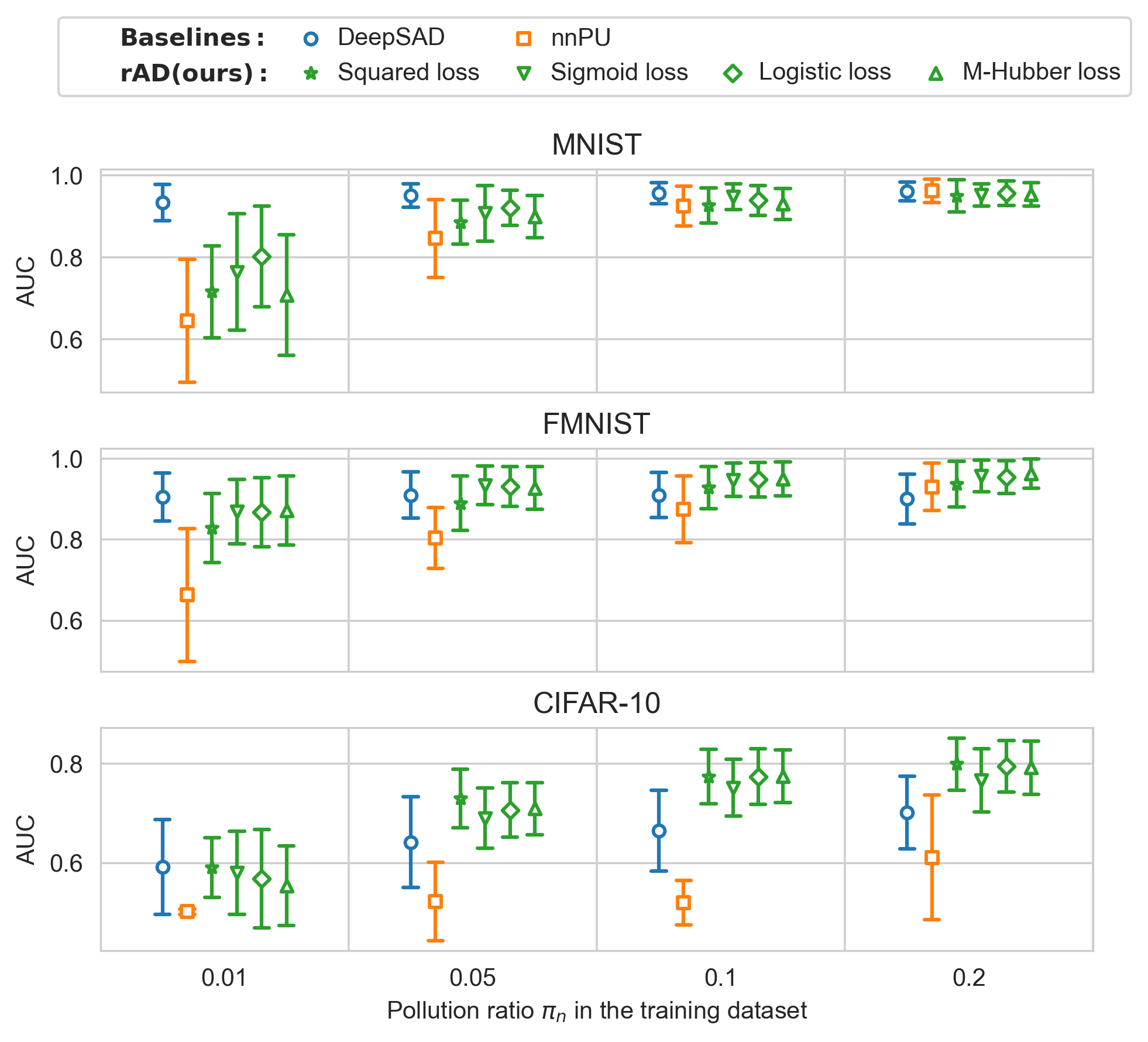
Figure 1: AUC mean and std over 20 trials with various $\pi_{n}$ and default $\gamma_{l}=0.05$

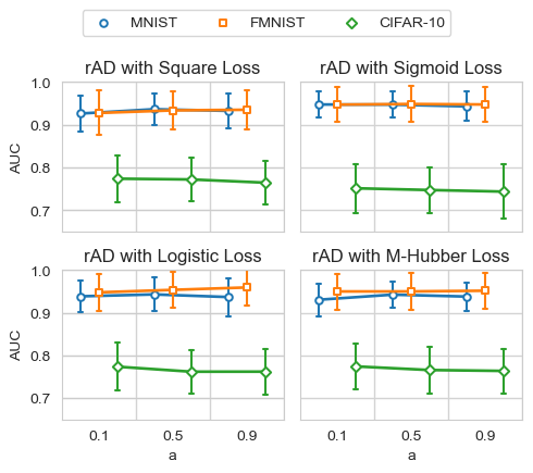
Figure 2: AUC mean and std over 20 trials at various $a$ for the datasets with $\gamma_{l}=0.05$ and $\pi_{n}=0.1$

To observe the impact of the amount of labeled data, we report the results for the datasets with $\pi_{n}=0.1$ and $\gamma_{l}\in\{0.05,0.1,0.2\}$ in Figure 5 in the supp. material. We observe that all the methods improve when we increase $\gamma_{l}$. From $\gamma_{l}=0.05$ to $\gamma_{l}=0.1$ (i.e., 5% more labeled data), deep rAD methods show a significant improvement in performance.

Sensitivity analysis for $\pi^{e}_{p}$ We run deep rAD with $a=0.1$ on the 20 trials of each dataset for $\pi_{p}^{e}\in\{1-\pi_{n},0.9,0.7,\pi_{n}\}$ (when $\pi_{p}^{e}=1-\pi_{n}$, it is an exact estimation of $\pi_{p}$, and when $\pi_{p}^{e}=\pi_{n}$, we can say $\pi_{p}^{e}$ is a bad estimation of $\pi_{p}$). We report the result in Table 6 in the supp. material. Again, we see that $\pi_{p}^{e}$ is not necessarily a precise estimation of $\pi_{p}$; and $(a,\pi_{p}^{e})=(0.1,0.8)$ or $(a,\pi_{p}^{e})=(0.1,0.7)$ are good settings. These results are consistent with the results of shallow rAD.

Sensitivity analysis for $a$ We fix $\pi_{p}^{e}=0.8$ and run deep rAD with additional values of $a\in\{0.5,0.9\}$ ($a=0.1$ is the default setting). We report the results for the datasets with $\pi_{n}=0.1$ and $\gamma_{l}=0.05$ in Figure 2. The results for the datasets with other values of $\pi_{n}$ and $\gamma_{l}$ are given in the supp. material. We observe that on CIFAR-10, AUC decreases when $a$ is increased; however, the difference is not significant. On FMNIST and MNIST, deep rAD with $\pi_{p}^{e}=0.8$ is quite robust to the change of $a$.

7 Limitations

Although the experiments have shown that our rAD methods are quite robust to the changes of the parameters $a$ and $\pi_{p}^{e}$, we still have to tune them to obtain the best AD performance. On the theoretical side, although the risk bounds are established for the proposed risk minimizers in Section 4, we still need the assumption that $\pi_{p}$ and $\pi_{n}$ are known in advance, which is a limitation.

8 Conclusion

With semi-supervised classification based on risk estimators, we have introduced a shallow AD method equipped with suitable regularization as well as a deep AD method. Theoretically, we have established the estimation error bounds and the excess risk bounds for the two risk minimizers. Empirically, the shallow AD methods show significant improvement over the baseline methods while the deep AD methods compete favorably with the baselines. Let us conclude the paper by giving some possible future research directions that address the limitation given in Section 7. One possible research direction is to develop a method that can learn the best combination of $(a,\pi_{p}^{e})$ from the available data. On the other hand, our experiments have shown that using $a=0.1$, precise estimation of $\pi_{p}$ and $\pi_{n}$ are not necessarily needed to obtain good accuracy in terms of AUC. Hence, another possible research direction would be to study the theoretical bounds of the risk minimizers with $\pi_{p}$ and $\pi_{n}$ replaced by some estimates.

Supplementary material

Appendix A Technical proofs

A.1 Proof of Theorem 1

(i) We have

$$\begin{split}&\frac{\pi_{n}}{n_{n}}\sum_{i=1}^{n_{n}}\ell(g(x_{i}^{n}),-1)-\frac{a\pi_{n}}{n_{n}}\sum_{i=1}^{n_{n}}\ell(g(x_{i}^{n}),+1)\\ &=(1-a)\frac{\pi_{n}}{n_{n}}\sum_{i=1}^{n_{n}}\ell(g(x_{i}^{n}),-1)+\frac{a\pi_{n}}{n_{n}}\sum_{i=1}^{n_{n}}(\ell(g(x_{i}^{n}),-1)-\ell(g(x_{i}^{n}),+1))\\ &\geq(1-a)\frac{\pi_{n}}{n_{n}}\sum_{i=1}^{n_{n}}b_{2}(b_{3}-|g(x_{i}^{n})|)-a\frac{\pi_{n}}{n_{n}}\sum_{i=1}^{n_{n}}b_{1}|g(x_{i}^{n})|\\ &=(1-a)\pi_{n}b_{2}b_{3}-((1-a)b_{2}+ab_{1})\frac{\pi_{n}}{n_{n}}\sum_{i=1}^{n_{n}}|g(x_{i}^{n})|.\end{split}$$

(ii) We have (17) is a direct consequence of Theorem 1(i).

(iii) Considering the first case, $\lambda\geq\frac{((1-a)b_{2}+ab_{1})^{2}\pi_{n}c^{2}}{4(1-a)b_{2}b_{3}}$ and $\mathbf{R}(w)=\|w\|_{2}^{2}$, we have

$$\begin{split}\lambda\mathbf{R}(w)+(1-a)\pi_{n}b_{2}b_{3}&\stackrel{{\scriptstyle\rm(a)}}{{\geq}}\frac{((1-a)b_{2}+ab_{1})^{2}}{4(1-a)b_{2}b_{3}}\frac{\pi_{n}}{n_{n}^{2}}(\sum_{i=1}^{n_{n}}|g(x_{i}^{n})|)^{2}+(1-a)\pi_{n}b_{2}b_{3}\\ &\stackrel{{\scriptstyle\rm(b)}}{{\geq}}((1-a)b_{2}+ab_{1})\frac{\pi_{n}}{n_{n}}\sum_{i=1}^{n_{n}}|g(x_{i}^{n})|,\end{split}$$

where in (a) we used the property that $|g(x_{i}^{n})|=|\langle w,\phi(x_{i}^{n})\rangle|\leq c\|w\|_{2}$, and in (b) we used the inequality $u+v\geq 2\sqrt{uv}$ for all nonnegative $u$ and $v$.

Consider the second case, $\mathbf{R}(w)=\|w\|_{1}$ and $\lambda\geq c_{\infty}((1-a)b_{2}+ab_{1})\pi_{n}$. Note that $|g(x_{i}^{n})|=|\langle w,\phi(x_{i}^{n})\rangle|\leq c_{\infty}\|w\|_{1}$. Hence, we have

$$\begin{split}\lambda\mathbf{R}(w)+(1-a)\pi_{n}b_{2}b_{3}&>c_{\infty}((1-a)b_{2}+ab_{1})\pi_{n}\|w\|_{1}\geq((1-a)b_{2}+ab_{1})\frac{\pi_{n}}{n_{n}}\sum_{i=1}^{n_{n}}|g(x_{i}^{n})|.\end{split}$$

Derivation of $b_{1}$, $b_{2}$ and $b_{3}$ in Table 1

Hinge loss. We have

$$\begin{split}\ell(t,-1)-\ell(t,+1)&=\max\{0,1+t\}-\max\{0,1-t\}=\begin{cases}t-1&\mbox{if}\,t<-1,\\ 2t&\mbox{if}\,-1\leq t\leq 1,\\ 1+t&\mbox{if}\,t>1,\end{cases}\\ &\geq-2|t|,\end{split}$$

and

$$\begin{split}\ell(t,-1)-b_{2}(1-|t|)=\max\{0,1+t\}-b_{2}(1-|t|)=\begin{cases}-b_{2}(1+t)&\mbox{if}\,t<-1,\\ t+1-b_{2}-b_{2}t&\mbox{if}\,-1\leq t\leq 0,\\ 1+t-b_{2}+b_{2}t&\mbox{if}\,t>0,\end{cases}\end{split}$$

Hence, the hinge loss with $b_{1}=2$, $b_{2}=1$ and $b_{3}=1$ satisfies (16).

Double hinge loss. Similarly, we have

$$\begin{split}\ell(t,-1)-\ell(t,+1)&=\max\{0,(1+t)/2,t\}-\max\{0,(1-t)/2,-t\}=t\geq-|t|,\end{split}$$

and

$$\begin{split}\ell(t,-1)-b_{2}(1-|t|)&=\max\{0,(1+t)/2,t\}-b_{2}(1-|t|)\\ &=\begin{cases}-b_{2}(1+t)&\mbox{if}\,t<-1,\\ t/2+1/2-b_{2}-b_{2}t&\mbox{if}\,-1\leq t\leq 0,\\ t/2+1/2-b_{2}+b_{2}t&\mbox{if}\,0<t\leq 1,\\ t-b_{2}+b_{2}t&\mbox{if}\,t>1.\end{cases}\end{split}$$

Hence, the double hinge loss with $b_{1}=1$, $b_{2}=1/2$ and $b_{3}=1$ satisfies (16).

Square loss. We have

$$\begin{split}\ell(t,-1)-\ell(t,+1)=\frac{1}{2}(t+1)^{2}-\frac{1}{2}(t-1)^{2}=2t\geq-2|t|.\end{split}$$

Note that when $|t|>1$ we have $(1/2-|t|)<0$, which implies $\ell(t,-1)-1/2(1/2-|t|)>0$. Considering $|t|\leq 1$, when $b_{2}=1/2$ and $b_{3}=1/2$, we have

$$\begin{split}\ell(t,-1)-1/2(1/2-|t|)&=1/2(t+1)^{2}-1/2(1/2-|t|)=\begin{cases}t^{2}+3/2t+1/4&\mbox{if}\,0\leq t\leq 1\\ t^{2}+1/2t+1/4&\mbox{if}\,-1\leq t\leq 0.\end{cases}\end{split}$$

Hence, the square loss with$b_{1}=2$, $b_{2}=1/2$, $b_{3}=1/2$ satisfies (16).4

Modified Huber loss. We have

$$\begin{split}\ell(t,-1)-\ell(t,+1)&=\begin{cases}\max\{0,1+t\}^{2}&\mbox{if}\,t\leq 1\\ 4t&\mbox{if}\,t>1\end{cases}-\begin{cases}\max\{0,1-t\}^{2}&\mbox{if}\,t\geq-1\\ -4t&\mbox{if}\,t<-1\end{cases}\\ &=4t\geq-4|t|.\end{split}$$

Considering $|t|\leq 1$, when $b_{2}=1$, $b_{3}=1/2$, we have

$$\begin{split}\ell(t,-1)-(1/2-|t|)&=\begin{cases}\max\{0,1+t\}^{2}&\mbox{if}\,t\leq 1\\ 4t&\mbox{if}\,t>1\end{cases}-b_{2}(1/2-|t|)\\ &=\begin{cases}t^{2}+1/2+t&\mbox{if}\,-1\leq t\leq 0\\ t^{2}+5/2t+1/2&\mbox{if}\,0<t\leq 1\end{cases}.\end{split}$$

Hence the modified Huber loss with $b_{1}=4$, $b_{2}=1$ and $b_{3}=1/2$ satisfies (16).

Logistic loss. We have

$$\begin{split}\ell(t,-1)-\ell(t,+1)=t\geq-|t|.\end{split}$$

When $t\geq 0$ then $\ln(1+\exp(t))\geq\ln 2=b_{3}\geq b_{3}-|t|$. When $t\leq 0$ we have

$$\begin{split}\ell(t,-1)-b_{2}(b_{3}-|t|)&=\ln(1+\exp(t))-(\ln 2+t)\\ &=\ln\big{(}\frac{1+\exp(t)}{2\exp(t)}\big{)}\geq\ln 1=0.\end{split}$$

Hence the logistic loss with $b_{1}=1$, $b_{2}=1$ and $b_{3}=\ln 2$ satisfies (16).

Sigmoid loss. When $t>0$, we have $\ell(t,-1)=\frac{1}{1+\exp(-t)}\geq 1/2\geq b_{2}(1-|t|)$. For $t\leq 0$, we have

$$\begin{split}\ell(t,-1)-b_{2}(1-|t|)=\frac{1}{1+\exp(-t)}-1/2(1+t)=\frac{1-1/2(1+\exp(-t))(1+t)}{1+\exp(-t)}.\end{split}$$

Note that the function $t\mapsto 1/2(1+\exp(-t))(1+t)$ is an increasing function on $(-\infty,0]$ and its maximum value on $(-\infty,0]$ is 1. Hence $\ell(t,-1)\geq 1/2(1-|t|)$. On the other hand, we have

$$\begin{split}\ell(t,-1)-\ell(t,+1)=2\ell(t,-1)-1\geq-|t|.\end{split}$$

Hence, the sigmoid loss with $b_{1}=1$, $b_{2}=1/2$ and $b_{3}=1$ satisfies (16).

Ramp loss. We have

$$\begin{split}\ell(t,-1)-b_{2}(b_{3}-|t|)&=\max\{0,\min\{1,(1+t)/2\}\}-1/2(1-|t|)\\ &=\begin{cases}-1/2(1+t)&\mbox{if}\,t\leq-1\\ 0&\mbox{if}\,-1\leq t\leq 0\\ t&\mbox{if}\,0<t\leq 1\\ 1/2+1/2t&\mbox{if}\,t\geq 1.\end{cases}\end{split}$$

Hence, $\ell(t,-1)\geq 1/2(1-|t|)$. On the other hand, we have

$$\begin{split}\ell(t,-1)-\ell(t,+1)=2\ell(t,-1)-1\geq-|t|.\end{split}$$

Hence, the ramp loss with $b_{1}=1$, $b_{2}=1/2$ and $b_{3}=1$ satisfies (16).

A.2 Proof of Proposition 1

Proof of Inequality (21)

Note that $\operatorname{\mathbb{E}}[\hat{\mathcal{R}}^{2}_{s}(g)]=\mathcal{R}(g)$. Considering $\hat{\mathcal{R}}^{1}_{s}(g)$, we have $\hat{\mathcal{R}}^{1}_{s}(g)=\hat{\mathcal{R}}^{2}_{s}(g)$ on

$$\mathcal{M}^{+}(g):=\{(\mathcal{N},\mathcal{U}):\hat{\mathcal{R}}^{+}_{u}(g)-\pi_{n}\hat{\mathcal{R}}^{+}_{n}(g)\geq 0\}.$$

Denote $\mathcal{M}^{-}(g):=\{(\mathcal{N},\mathcal{U}):\hat{\mathcal{R}}^{+}_{u}(g)-\pi_{n}\hat{\mathcal{R}}^{+}_{n}(g)<0\}$. We have

$$\begin{split}\operatorname{\mathbb{E}}[\hat{\mathcal{R}}^{1}_{s}(g)]-\mathcal{R}(g)&=\operatorname{\mathbb{E}}[\hat{\mathcal{R}}^{1}_{s}(g)-\hat{\mathcal{R}}^{2}_{s}(g)]\\ &=\int_{(\mathcal{N},\mathcal{U})\in\mathcal{M}^{-}(g)}\big{(}\hat{\mathcal{R}}^{1}_{s}(g)-\hat{\mathcal{R}}^{2}_{s}(g)\big{)}dF(\mathcal{N},\mathcal{U})\\ &=\int_{(\mathcal{N},\mathcal{U})\in\mathcal{M}^{-}(g)}a\big{(}\pi_{n}\hat{\mathcal{R}}^{+}_{n}(g)-\hat{\mathcal{R}}^{+}_{u}(g)\big{)}dF(\mathcal{N},\mathcal{U})\qquad(\ref{proof1:temp1}a)\\ &\leq\sup_{(\mathcal{N},\mathcal{U})\in\mathcal{M}^{-}(g)}a\big{(}\pi_{n}\hat{\mathcal{R}}^{+}_{n}(g)-\hat{\mathcal{R}}^{+}_{u}(g)\big{)}\int_{(\mathcal{N},\mathcal{U})\in\mathcal{M}^{-}(g)}dF(\mathcal{N},\mathcal{U})\\ &=a\sup_{(\mathcal{N},\mathcal{U})\in\mathcal{M}^{-}(g)}\big{(}\pi_{n}\hat{\mathcal{R}}^{+}_{n}(g)-\hat{\mathcal{R}}^{+}_{u}(g)\big{)}{\rm Pr}(\mathcal{M}^{-}(g))\\ &\leq a\pi_{n}C_{\ell}{\rm Pr}(\mathcal{M}^{-}(g)).\end{split}$$ (26)

From (26a) we have $\operatorname{\mathbb{E}}[\hat{\mathcal{R}}^{1}_{s}(g)]-\mathcal{R}(g)\geq 0$. On the other hand,

$$\begin{split}{\rm Pr}(\mathcal{M}^{-}(g))&={\rm Pr}\big{(}\hat{\mathcal{R}}^{+}_{u}(g)-\pi_{n}\hat{\mathcal{R}}^{+}_{n}(g)<0\big{)}\\ &\leq{\rm Pr}\big{(}\hat{\mathcal{R}}^{+}_{u}(g)-\pi_{n}\hat{\mathcal{R}}^{+}_{n}(g)\leq\pi_{p}\mathcal{R}_{p}^{+}(g)-\pi_{p}\rho_{g}\big{)}\\ &={\rm Pr}\big{(}\pi_{p}\mathcal{R}_{p}^{+}(g)-(\hat{\mathcal{R}}^{+}_{u}(g)-\pi_{n}\hat{\mathcal{R}}^{+}_{n}(g))\geq\pi_{p}\rho_{g}\big{)}\\ &\leq\exp\left(-\frac{2(\pi_{p}\rho_{g})^{2}}{n_{u}(C_{\ell}/n_{u})^{2}+n_{n}(\pi_{n}C_{\ell}/n_{n})^{2}}\right)\\ &=\exp\left(-\frac{2\pi_{p}^{2}\rho_{g}^{2}}{C_{\ell}^{2}(1/n_{u}+\pi_{n}^{2}/n_{n})}\right),\end{split}$$

where we have used McDiarmid’s inequality for the last inequality. Therefore, from (26) we have

$$\begin{split}\operatorname{\mathbb{E}}[\hat{\mathcal{R}}^{1}_{s}(g)]-\mathcal{R}(g)\leq a\pi_{n}C_{\ell}\exp\left(-\frac{2\pi_{p}^{2}\rho_{g}^{2}}{C_{\ell}^{2}(1/n_{u}+\pi_{n}^{2}/n_{n})}\right).\end{split}$$ (27)

Proof of Inequality (22) and (23)

If an $x_{i}^{n}$ is changed then the change of $\hat{\mathcal{R}}^{1}_{s}(g)$ would be no more than $\pi_{n}(a+1)C_{\ell}/n_{n}$. If an $x_{i}^{u}$ is changed then the change of $\hat{\mathcal{R}}^{1}_{s}(g)$ would be no more than $aC_{\ell}/n_{u}$. And if an $x_{i}^{p}$ is changed then the change of $\hat{\mathcal{R}}^{1}_{s}(g)$ would be no more than $(1-a)\pi_{p}C_{\ell}/n_{p}$. For any $\delta>0$, let

$$\varepsilon=C_{\ell}\sqrt{\big{(}\frac{(1+a)^{2}\pi_{n}^{2}}{n_{n}}+\frac{(1-a)^{2}\pi_{p}^{2}}{n_{p}}+\frac{a^{2}}{n_{u}}\big{)}\ln(2/\delta)/2}.$$

Applying McDiarmid’s inequality, we get

$$\begin{split}&{\rm Pr}(|\hat{\mathcal{R}}^{1}_{s}(g)-\operatorname{\mathbb{E}}[\hat{\mathcal{R}}^{1}_{s}(g)]|\geq\varepsilon)\\ &\leq 2\exp\left(-\frac{2\varepsilon^{2}}{n_{n}(\pi_{n}(1+a)C_{l}/n_{n})^{2}+n_{p}((1-a)\pi_{p}C_{l}/n_{p})^{2}+n_{u}(aC_{\ell}/n_{u})^{2}}\right)\\ &=\delta.\end{split}$$ (28)

Hence,

$$|\hat{\mathcal{R}}^{1}_{s}(g)-\operatorname{\mathbb{E}}[\hat{\mathcal{R}}^{1}_{s}(g)]|\leq\varepsilon\leq C_{\ell}\sqrt{\ln(2/\delta)/2}\big{(}\frac{(1+a)\pi_{n}}{\sqrt{n_{n}}}+\frac{(1-a)\pi_{p}}{\sqrt{n_{p}}}+\frac{a}{\sqrt{n_{u}}}\big{)}$$

with probability at least $1-\delta$. Together with (27) and

$$\begin{split}|\hat{\mathcal{R}}^{1}_{s}(g)-\mathcal{R}(g)|\leq|\hat{\mathcal{R}}^{1}_{s}(g)-\operatorname{\mathbb{E}}[\hat{\mathcal{R}}^{1}_{s}(g)]|+|\operatorname{\mathbb{E}}[\hat{\mathcal{R}}^{1}_{s}(g)]-\mathcal{R}(g)|,\end{split}$$

we obtain Inequality (23) with probability at least $1-\delta$.

Similarly, by applying McDiarmid’s inequality, we obtain Inequality (22) with probability at least $1-\delta$.

A.3 Proof of Theorem 2

Denote $\tilde{\mathcal{R}}_{nu}(g)=\pi_{n}\hat{\mathcal{R}}^{-}_{n}(g)+a\max\{0,\hat{\mathcal{R}}^{+}_{u}(g)-\pi_{n}\hat{\mathcal{R}}^{+}_{n}(g)\}$. Note that

$$\hat{\mathcal{R}}^{1}_{s}(g)=(1-a)\pi_{p}\hat{\mathcal{R}}_{p}^{+}+\tilde{\mathcal{R}}_{nu}(g).$$

We have

$$\begin{split}\mathcal{R}(\hat{g}^{1})-\mathcal{R}(g^{*})&=\mathcal{R}(\hat{g}^{1})-\hat{\mathcal{R}}^{1}_{s}(\hat{g}^{1})+\hat{\mathcal{R}}^{1}_{s}(\hat{g}^{1})-\hat{\mathcal{R}}^{1}_{s}(g^{*})+\hat{\mathcal{R}}^{1}_{s}(g^{*})-\mathcal{R}(g^{*})\\ &\stackrel{{\scriptstyle\rm(a)}}{{\leq}}|\hat{\mathcal{R}}^{1}_{s}(\hat{g}^{1})-\mathcal{R}(\hat{g}^{1})|+|\hat{\mathcal{R}}^{1}_{s}(g^{*})-\mathcal{R}(g^{*})|\\ &\leq 2\sup_{g\in\mathcal{G}}|\hat{\mathcal{R}}^{1}_{s}(g)-\mathcal{R}(g)|\\ &\leq 2\big{(}\sup_{g\in\mathcal{G}}\big{|}\hat{\mathcal{R}}^{1}_{s}(g)-\operatorname{\mathbb{E}}[\hat{\mathcal{R}}^{1}_{s}(g)]\big{|}+\sup_{g\in\mathcal{G}}\big{|}\operatorname{\mathbb{E}}[\hat{\mathcal{R}}^{1}_{s}(g)]-\mathcal{R}(g)\big{|}\big{)}\\ &\stackrel{{\scriptstyle\rm(b)}}{{\leq}}2\sup_{g\in\mathcal{G}}\big{|}\hat{\mathcal{R}}^{1}_{s}(g)-\operatorname{\mathbb{E}}[\hat{\mathcal{R}}^{1}_{s}(g)]\big{|}+2\epsilon\\ &\leq 2(1-a)\pi_{p}\sup_{g\in\mathcal{G}}\big{|}\hat{\mathcal{R}}_{p}^{+}-\operatorname{\mathbb{E}}[\hat{\mathcal{R}}_{p}^{+}]\big{|}+2\sup_{g\in\mathcal{G}}\big{|}\tilde{\mathcal{R}}_{nu}(g)-\operatorname{\mathbb{E}}[\tilde{\mathcal{R}}_{nu}(g)]\big{|}+2\epsilon,\end{split}$$ (29)

where we used $\hat{\mathcal{R}}^{1}_{s}(\hat{g}^{1})-\hat{\mathcal{R}}^{1}_{s}(g^{*})\leq 0$ for (a), and used (21) for (b).

To obtain a bound for $\sup_{g\in\mathcal{G}}\big{|}\tilde{\mathcal{R}}_{nu}(g)-\operatorname{\mathbb{E}}[\tilde{\mathcal{R}}_{nu}(g)]\big{|}$ we adapt the technique of (Kiryo et al., 2017, Theorem 4). Note that for a fix $g$, $\operatorname{\mathbb{E}}[\tilde{\mathcal{R}}_{nu}(g)]$ is a constant. Hence, if an $x_{i}^{n}$, or $x_{i}^{u}$ is changed then the change of $\sup_{g\in\mathcal{G}}\big{|}\tilde{\mathcal{R}}_{nu}(g)-\operatorname{\mathbb{E}}[\tilde{\mathcal{R}}_{nu}(g)]\big{|}$ would be the supremum of the change of $\tilde{\mathcal{R}}_{nu}(g)$. By applying McDiarmid’s inequality to $\sup_{g\in\mathcal{G}}\big{|}\tilde{\mathcal{R}}_{nu}(g)-\operatorname{\mathbb{E}}[\tilde{\mathcal{R}}_{nu}(g)]\big{|}$, we have

$$\begin{split}&\sup_{g\in\mathcal{G}}\big{|}\tilde{\mathcal{R}}_{nu}(g)-\operatorname{\mathbb{E}}[\tilde{\mathcal{R}}_{nu}(g)]\big{|}-\operatorname{\mathbb{E}}\big{[}\sup_{g\in\mathcal{G}}\big{|}\tilde{\mathcal{R}}_{nu}(g)-\operatorname{\mathbb{E}}[\tilde{\mathcal{R}}_{nu}(g)]\big{|}\big{]}\\ &\quad\leq C_{\ell}\sqrt{\ln(2/\delta)/2}\big{(}\frac{(1+a)\pi_{n}}{\sqrt{n_{n}}}+\frac{a}{\sqrt{n_{u}}}\big{)}\end{split}$$ (30)

with probability at least $1-\delta/2$.

Let $(\mathcal{N}^{\prime},\mathcal{U}^{\prime})$ be a ghost sample identical to $(\mathcal{N},\mathcal{U})$. We have

$$\begin{split}&\operatorname{\mathbb{E}}\big{[}\sup_{g\in\mathcal{G}}\big{|}\tilde{\mathcal{R}}_{nu}(g)-\operatorname{\mathbb{E}}[\tilde{\mathcal{R}}_{nu}(g)]\big{|}\big{]}\\ &=\operatorname{\mathbb{E}}_{(\mathcal{N},\mathcal{U})}\big{[}\sup_{g\in\mathcal{G}}\big{|}\tilde{\mathcal{R}}_{nu}(g;\mathcal{N},\mathcal{U})-\operatorname{\mathbb{E}}_{(\mathcal{N}^{\prime},\mathcal{U}^{\prime})}[\tilde{\mathcal{R}}_{nu}(g;\mathcal{N}^{\prime},\mathcal{U}^{\prime})]\big{|}\big{]}\\ &=\operatorname{\mathbb{E}}_{(\mathcal{N},\mathcal{U})}\big{[}\sup_{g\in\mathcal{G}}\big{|}\operatorname{\mathbb{E}}_{(\mathcal{N}^{\prime},\mathcal{U}^{\prime})}[\tilde{\mathcal{R}}_{nu}(g;\mathcal{N},\mathcal{U})-\tilde{\mathcal{R}}_{nu}(g;\mathcal{N}^{\prime},\mathcal{U}^{\prime})]\big{|}\big{]}\\ &\leq\operatorname{\mathbb{E}}_{(\mathcal{N},\mathcal{U}),(\mathcal{N}^{\prime},\mathcal{U}^{\prime})}\big{[}\sup_{g\in\mathcal{G}}\big{|}\tilde{\mathcal{R}}_{nu}(g;\mathcal{N},\mathcal{U})-\tilde{\mathcal{R}}_{nu}(g;\mathcal{N}^{\prime},\mathcal{U}^{\prime})\big{|}\big{]},\end{split}$$ (31)

where we applied Jensen’s inequality. Furthermore, we have

$$\begin{split}&\big{|}\tilde{\mathcal{R}}_{nu}(g;\mathcal{N},\mathcal{U})-\tilde{\mathcal{R}}_{nu}(g;\mathcal{N}^{\prime},\mathcal{U}^{\prime})\big{|}\\ &\leq\pi_{n}\big{|}\hat{\mathcal{R}}_{n}^{-}(g;\mathcal{N})-\hat{\mathcal{R}}_{n}^{-}(g;\mathcal{N}^{\prime})\big{|}\\ &\qquad+a\big{|}\max\{0,\hat{\mathcal{R}}^{+}_{u}(g;\mathcal{U})-\pi_{n}\hat{\mathcal{R}}^{+}_{n}(g;\mathcal{N})\}-\max\{0,\hat{\mathcal{R}}^{+}_{u}(g;\mathcal{U}^{\prime})-\pi_{n}\hat{\mathcal{R}}^{+}_{n}(g;\mathcal{N}^{\prime})\}\big{|}\\ &\leq\pi_{n}\big{|}\hat{\mathcal{R}}_{n}^{-}(g;\mathcal{N})-\hat{\mathcal{R}}_{n}^{-}(g;\mathcal{N}^{\prime})\big{|}\\ &\qquad+a\big{|}\hat{\mathcal{R}}^{+}_{u}(g;\mathcal{U})-\hat{\mathcal{R}}^{+}_{u}(g;\mathcal{U}^{\prime})\big{|}+a\pi_{n}\big{|}\hat{\mathcal{R}}^{+}_{n}(g;\mathcal{N})-\hat{\mathcal{R}}^{+}_{n}(g;\mathcal{N}^{\prime})\big{|}.\end{split}$$ (32)

Hence, from (31) and (32), we obtain

$$\begin{split}&\operatorname{\mathbb{E}}\big{[}\sup_{g\in\mathcal{G}}\big{|}\tilde{\mathcal{R}}_{nu}(g)-\operatorname{\mathbb{E}}[\tilde{\mathcal{R}}_{nu}(g)]\big{|}\big{]}\\ &\leq\pi_{n}\operatorname{\mathbb{E}}_{\mathcal{N},\mathcal{N}^{\prime}}\big{[}\sup_{g\in\mathcal{G}}\big{|}\hat{\mathcal{R}}^{-}_{n}(g;\mathcal{N})-\hat{\mathcal{R}}^{-}_{n}(g;\mathcal{N}^{\prime})\big{|}\big{]}+a\operatorname{\mathbb{E}}_{\mathcal{U},\mathcal{U}^{\prime}}\big{[}\sup_{g\in\mathcal{G}}\big{|}\hat{\mathcal{R}}^{+}_{u}(g;\mathcal{U})-\hat{\mathcal{R}}^{+}_{u}(g;\mathcal{U}^{\prime})\big{|}\big{]}\\ &\quad+a\pi_{n}\operatorname{\mathbb{E}}_{\mathcal{N},\mathcal{N}^{\prime}}\big{[}\sup_{g\in\mathcal{G}}\big{|}\hat{\mathcal{R}}^{+}_{n}(g;\mathcal{N})-\hat{\mathcal{R}}^{+}_{n}(g;\mathcal{N}^{\prime})\big{|}\big{]}.\end{split}$$ (33)

Now by using the same technique of (Kiryo et al., 2017, Lemma 5), we can prove that

$$\begin{split}\operatorname{\mathbb{E}}_{\mathcal{N},\mathcal{N}^{\prime}}\big{[}\sup_{g\in\mathcal{G}}\big{|}\hat{\mathcal{R}}^{-}_{n}(g;\mathcal{N})-\hat{\mathcal{R}}^{-}_{n}(g;\mathcal{N}^{\prime})\big{|}\big{]}&\leq 4L_{\ell}\mathfrak{R}_{n_{n},p_{n}}(\mathcal{G}),\\ \operatorname{\mathbb{E}}_{\mathcal{U},\mathcal{U}^{\prime}}\big{[}\sup_{g\in\mathcal{G}}\big{|}\hat{\mathcal{R}}^{+}_{u}(g;\mathcal{U})-\hat{\mathcal{R}}^{+}_{u}(g;\mathcal{U}^{\prime})\big{|}\big{]}&\leq 4L_{\ell}\mathfrak{R}_{n_{u},p}(\mathcal{G}),\\ \operatorname{\mathbb{E}}_{\mathcal{N},\mathcal{N}^{\prime}}\big{[}\sup_{g\in\mathcal{G}}\big{|}\hat{\mathcal{R}}^{+}_{n}(g;\mathcal{N})-\hat{\mathcal{R}}^{+}_{n}(g;\mathcal{N}^{\prime})\big{|}\big{]}&\leq 4L_{\ell}\mathfrak{R}_{n_{n},p_{n}}(\mathcal{G}).\end{split}$$ (34)

For completeness, let us provide the proof in the following.

Denote $\tilde{\ell}(t,y)=\ell(t,y)-\ell(0,y)$. Then, $\tilde{\ell}(0,y)=0$. Note that $t\mapsto\tilde{\ell}(t,y)$ is also $L_{\ell}$-Lipschitz continuous over $\{t:|t|\leq C_{g}\}$. Denote $\mathfrak{R}^{\prime}_{n,q}(\mathcal{G}):=\operatorname{\mathbb{E}}_{Z\sim q^{n}}[\operatorname{\mathbb{E}}_{\sigma}[\sup_{g\in\mathcal{G}}|\frac{1}{n}\sum_{i=1}^{n}\sigma_{i}g(Z_{i})|]]$. We prove the first inequality of (34), the others can be proved similarly. We have

$$\begin{split}&\operatorname{\mathbb{E}}_{\mathcal{N},\mathcal{N}^{\prime}}\big{[}\sup_{g\in\mathcal{G}}\big{|}\hat{\mathcal{R}}^{-}_{n}(g;\mathcal{N})-\hat{\mathcal{R}}^{-}_{n}(g;\mathcal{N}^{\prime})\big{|}\big{]}\\ &=\operatorname{\mathbb{E}}_{\mathcal{N},\mathcal{N}^{\prime}}\big{[}\sup_{g\in\mathcal{G}}\big{|}\frac{1}{n_{n}}\sum_{i=1}^{n_{n}}\ell(g(x_{i}^{n}),-1)-\frac{1}{n_{n}}\sum_{i=1}^{n_{n}}\ell(g({x^{\prime}}_{i}^{n}),-1)\big{|}\big{]}\\ &=\operatorname{\mathbb{E}}_{\mathcal{N},\mathcal{N}^{\prime}}\big{[}\sup_{g\in\mathcal{G}}\big{|}\frac{1}{n_{n}}\sum_{i=1}^{n_{n}}\big{(}\tilde{\ell}(g(x_{i}^{n}),-1)-\tilde{\ell}(g({x^{\prime}}_{i}^{n}),-1)\big{)}\big{|}\big{]}\\ &\stackrel{{\scriptstyle\rm(a)}}{{=}}\operatorname{\mathbb{E}}_{\mathcal{N},\mathcal{N}^{\prime},\sigma}\big{[}\sup_{g\in\mathcal{G}}\big{|}\frac{1}{n_{n}}\sum_{i=1}^{n_{n}}\sigma_{i}\big{(}\tilde{\ell}(g(x_{i}^{n}),-1)-\tilde{\ell}(g({x^{\prime}}_{i}^{n}),-1)\big{)}\big{|}\big{]}\\ &\leq 2\mathfrak{R}^{\prime}_{n_{n},p_{n}}(\tilde{\ell}(\cdot,-1)\circ\mathcal{G})\stackrel{{\scriptstyle\rm(b)}}{{\leq}}4L_{\ell}\mathfrak{R}^{\prime}_{n_{n},p_{n}}(\mathcal{G})\stackrel{{\scriptstyle\rm(c)}}{{=}}4L_{\ell}\mathfrak{R}_{n_{n},p_{n}}(\mathcal{G}),\end{split}$$

where in (a) we used the property that $\sigma_{i}$ are independent uniformly distributed random variables taking values in $\{-1,+1\}$, in (b) we use (Ledoux & Talagrand, 1991, Theorem 4.12), and in (c) we use the assumption that both $g$ and $-g$ are in $\mathcal{G}$.

On the other hand, in a similar manner, we can prove that

$$\sup_{g\in\mathcal{G}}\big{|}\hat{\mathcal{R}}_{p}^{+}-\operatorname{\mathbb{E}}[\hat{\mathcal{R}}_{p}^{+}]\big{|}\leq 4L_{\ell}\mathfrak{R}_{n_{p},p_{p}}(\mathcal{G})+C_{\ell}\frac{\sqrt{\ln(2/\delta)/2}}{\sqrt{n_{p}}}$$ (35)

with probability at least $1-\delta/2$. From (29), (30), (33), (34), and (35), we obtain the result.

A.4 Proof of Theorem 3

We have

$$\begin{split}\mathcal{R}(\hat{g}^{2})-\mathcal{R}(g^{*})&=\mathcal{R}(\hat{g}^{2})-\hat{\mathcal{R}}^{2}_{s}(\hat{g}^{2})+\hat{\mathcal{R}}^{2}_{s}(\hat{g}^{2})-\hat{\mathcal{R}}^{2}_{s}(g^{*})+\hat{\mathcal{R}}^{2}_{s}(g^{*})-\mathcal{R}(g^{*})\\ &\stackrel{{\scriptstyle\rm(a)}}{{\leq}}\mathcal{R}(\hat{g}^{2})-\hat{\mathcal{R}}^{2}_{s}(\hat{g}^{2})+\hat{\mathcal{R}}^{2}_{s}(g^{*})-\mathcal{R}(g^{*})\\ &\leq\sup_{g\in\mathcal{G}}\big{(}\mathcal{R}(g)-\hat{\mathcal{R}}^{2}_{s}(g)\big{)}+\sup_{g\in\mathcal{G}}\big{(}\hat{\mathcal{R}}^{2}_{s}(g)-\mathcal{R}(g)\big{)}\\ &\stackrel{{\scriptstyle\rm(b)}}{{=}}\sup_{g\in\mathcal{G}}\big{(}\operatorname{\mathbb{E}}[\hat{\mathcal{R}}^{2}_{s}(g)]-\hat{\mathcal{R}}^{2}_{s}(g)\big{)}+\sup_{g\in\mathcal{G}}\big{(}\hat{\mathcal{R}}^{2}_{s}(g)-\operatorname{\mathbb{E}}[\hat{\mathcal{R}}^{2}_{s}(g)]\big{)}\end{split}$$ (36)

where in (a) we have used $\hat{\mathcal{R}}^{2}_{s}(\hat{g}^{2})\leq\hat{\mathcal{R}}^{2}_{s}(g^{*})$ and in (b) we have used $\operatorname{\mathbb{E}}[\hat{\mathcal{R}}^{2}_{s}(g)]=\mathcal{R}(g)$ given $g$.

We have

$$\begin{split}\sup_{g\in\mathcal{G}}\big{(}\operatorname{\mathbb{E}}[\hat{\mathcal{R}}^{2}_{s}(g)]-\hat{\mathcal{R}}^{2}_{s}(g)\big{)}&\leq a\sup_{g\in\mathcal{G}}\big{(}\operatorname{\mathbb{E}}[\hat{\mathcal{R}}^{+}_{u}(g)]-\hat{\mathcal{R}}^{+}_{u}(g)\big{)}+(1-a)\pi_{p}\sup_{g\in\mathcal{G}}\big{(}\operatorname{\mathbb{E}}[\hat{\mathcal{R}}_{p}^{+}(g)]-\hat{\mathcal{R}}_{p}^{+}(g)\big{)}\\ &\quad\qquad+\sup_{g\in\mathcal{G}}\big{(}\operatorname{\mathbb{E}}[\pi_{n}\hat{\mathcal{R}}^{-}_{n}(g)-a\pi_{n}\hat{\mathcal{R}}^{+}_{n}]-(\pi_{n}\hat{\mathcal{R}}^{-}_{n}(g)-a\pi_{n}\hat{\mathcal{R}}^{+}_{n})\big{)},\end{split}$$ (37)

and

$$\begin{split}\sup_{g\in\mathcal{G}}\big{(}\hat{\mathcal{R}}^{2}_{s}(g)-\operatorname{\mathbb{E}}[\hat{\mathcal{R}}^{2}_{s}(g)]\big{)}&\leq a\sup_{g\in\mathcal{G}}\big{(}\hat{\mathcal{R}}^{+}_{u}(g)-\operatorname{\mathbb{E}}[\hat{\mathcal{R}}^{+}_{u}(g)]\big{)}+(1-a)\pi_{p}\sup_{g\in\mathcal{G}}\big{(}\hat{\mathcal{R}}_{p}^{+}(g)-\operatorname{\mathbb{E}}[\hat{\mathcal{R}}_{p}^{+}(g)]\big{)}\\ &\quad\qquad+\sup_{g\in\mathcal{G}}\big{(}(\pi_{n}\hat{\mathcal{R}}^{-}_{n}(g)-a\pi_{n}\hat{\mathcal{R}}^{+}_{n})-\operatorname{\mathbb{E}}[\pi_{n}\hat{\mathcal{R}}^{-}_{n}(g)-a\pi_{n}\hat{\mathcal{R}}^{+}_{n}]\big{)},\end{split}$$ (38)

Applying McDiarmid’s inequality to $\sup_{g\in\mathcal{G}}\big{(}\operatorname{\mathbb{E}}[\hat{\mathcal{R}}^{+}_{u}(g)]-\hat{\mathcal{R}}^{+}_{u}(g)\big{)}$ we have

$$\begin{split}\sup_{g\in\mathcal{G}}\big{(}\operatorname{\mathbb{E}}[\hat{\mathcal{R}}^{+}_{u}(g)]-\hat{\mathcal{R}}^{+}_{u}(g)\big{)}-\operatorname{\mathbb{E}}\big{[}\sup_{g\in\mathcal{G}}\big{(}\operatorname{\mathbb{E}}[\hat{\mathcal{R}}^{+}_{u}(g)]-\hat{\mathcal{R}}^{+}_{u}(g)\big{)}]\leq C_{\ell}\sqrt{\ln(6/\delta)/2}\frac{1}{\sqrt{n_{u}}}\end{split}$$ (39)

with probability at least $\delta/6$. Moreover, letting $\mathcal{U}^{\prime}$ be a ghost sample identical to $\mathcal{U}$, we have

$$\begin{split}\operatorname{\mathbb{E}}\big{[}\sup_{g\in\mathcal{G}}\big{(}\operatorname{\mathbb{E}}[\hat{\mathcal{R}}^{+}_{u}(g)]-\hat{\mathcal{R}}^{+}_{u}(g)\big{)}]&=\operatorname{\mathbb{E}}_{\mathcal{U}}\big{[}\sup_{g\in\mathcal{G}}\big{(}\operatorname{\mathbb{E}}_{\mathcal{U}^{\prime}}[\hat{\mathcal{R}}^{+}_{u}(g;\mathcal{U}^{\prime})]-\hat{\mathcal{R}}^{+}_{u}(g;\mathcal{U})\big{)}]\\ &\stackrel{{\scriptstyle\rm(a)}}{{\leq}}\operatorname{\mathbb{E}}_{\mathcal{U},\mathcal{U}^{\prime}}\big{[}\sup_{g\in\mathcal{G}}\big{(}\hat{\mathcal{R}}^{+}_{u}(g;\mathcal{U}^{\prime})-\hat{\mathcal{R}}^{+}_{u}(g;\mathcal{U})\big{)}\big{]}\\ &=\operatorname{\mathbb{E}}_{\mathcal{U},\mathcal{U}^{\prime}}\big{[}\sup_{g\in\mathcal{G}}\big{(}\frac{1}{n_{u}}\sum_{i=1}^{n_{u}}(\ell(g({x^{\prime}}_{i}^{u}),+1)-\ell(g(x_{i}^{u}),+1))\big{)}\big{]}\\ &\stackrel{{\scriptstyle\rm(b)}}{{\leq}}\operatorname{\mathbb{E}}_{\mathcal{U},\mathcal{U}^{\prime},\sigma}\big{[}\sup_{g\in\mathcal{G}}\big{(}\frac{1}{n_{u}}\sum_{i=1}^{n_{u}}\sigma_{i}(\ell(g({x^{\prime}}_{i}^{u}),+1)-\ell(g(x_{i}^{u}),+1))\big{)}\big{]}\\ &\leq 2L_{\ell}\mathfrak{R}_{n_{u},p}(\mathcal{G}).\end{split}$$

where we have used the sub-additivity of the supremum in (a) and the property of $\sigma$ in (b). Together with (39) we get

$$\sup_{g\in\mathcal{G}}\big{(}\operatorname{\mathbb{E}}[\hat{\mathcal{R}}^{+}_{u}(g)]-\hat{\mathcal{R}}^{+}_{u}(g)\big{)}\leq 2L_{\ell}\mathfrak{R}_{n_{u},p}(\mathcal{G})+C_{\ell}\sqrt{\ln(6/\delta)/2}\frac{1}{\sqrt{n_{u}}}$$ (40)

with probability at least $\delta/6$. Similarly, we can prove the following inequalities hold with a probability of at least $1-\delta/6$

$$\begin{split}&\sup_{g\in\mathcal{G}}\big{(}\hat{\mathcal{R}}^{+}_{u}(g)-\operatorname{\mathbb{E}}[\hat{\mathcal{R}}^{+}_{u}(g)]\big{)}\leq 2L_{\ell}\mathfrak{R}_{n_{u},p}(\mathcal{G})+C_{\ell}\sqrt{\ln(6/\delta)/2}\frac{1}{\sqrt{n_{u}}},\\ &\sup_{g\in\mathcal{G}}\big{(}\hat{\mathcal{R}}_{p}^{+}(g)-\operatorname{\mathbb{E}}[\hat{\mathcal{R}}_{p}^{+}(g)]\big{)}\leq 2L_{\ell}\mathfrak{R}_{n_{p},p_{p}}(\mathcal{G})+C_{\ell}\sqrt{\ln(6/\delta)/2}\frac{1}{\sqrt{n_{p}}},\\ &\sup_{g\in\mathcal{G}}\big{(}\operatorname{\mathbb{E}}[\hat{\mathcal{R}}_{p}^{+}(g)]-\hat{\mathcal{R}}_{p}^{+}(g)\big{)}\leq 2L_{\ell}\mathfrak{R}_{n_{p},p_{p}}(\mathcal{G})+C_{\ell}\sqrt{\ln(6/\delta)/2}\frac{1}{\sqrt{n_{p}}},\\ &\sup_{g\in\mathcal{G}}\big{(}\pi_{n}\hat{\mathcal{R}}^{-}_{n}(g)-a\pi_{n}\hat{\mathcal{R}}^{+}_{n}-\operatorname{\mathbb{E}}[\pi_{n}\hat{\mathcal{R}}^{-}_{n}(g)-a\pi_{n}\hat{\mathcal{R}}^{+}_{n}]\big{)}\\ &\qquad\qquad\leq 2L_{\ell}(1+a)\pi_{n}\mathfrak{R}_{n_{n},p_{n}}(\mathcal{G})+C_{\ell}(1+a)\pi_{n}\sqrt{\ln(6/\delta)/2}\frac{1}{\sqrt{n_{n}}},\\ &\sup_{g\in\mathcal{G}}\big{(}\operatorname{\mathbb{E}}[\pi_{n}\hat{\mathcal{R}}^{-}_{n}(g)-a\pi_{n}\hat{\mathcal{R}}^{+}_{n}]-\pi_{n}\hat{\mathcal{R}}^{-}_{n}(g)-a\pi_{n}\hat{\mathcal{R}}^{+}_{n}\big{)}\\ &\qquad\qquad\leq 2L_{\ell}(1+a)\pi_{n}\mathfrak{R}_{n_{n},p_{n}}(\mathcal{G})+C_{\ell}(1+a)\pi_{n}\sqrt{\ln(6/\delta)/2}\frac{1}{\sqrt{n_{n}}}.\end{split}$$ (41)

From (36), (37), (38), (40), and (41), we get the result.

Appendix B Some definitions

Definition 1

A loss $\ell$ is said to be classification-calibrated if, for any $\eta\neq\frac{1}{2}$, we have $H_{\ell}^{-}(\eta)>H_{\ell}(\eta)$, where

$$\begin{split}H_{\ell}(\eta)&=\inf_{\alpha\in\mathbb{R}}(\eta\ell(\alpha,+1)+(1-\eta)\ell(\alpha,-1)),\\ H^{-}_{\ell}(\eta)&=\inf_{\alpha\in\mathbb{R}:\alpha(\eta-\frac{1}{2})\leq 0}(\eta\ell(\alpha,+1)+(1-\eta)\ell(\alpha,-1))\end{split}$$

Examples of classification-calibrated loss include the scaled ramp loss, the hinge loss, and the exponential loss. (Bartlett et al., 2006, Theorem 1) shows that if $\ell$ is a classification-calibrated loss, then there exists a convex, invertible and nondecreasing transformation $\psi_{\ell}$ with $\psi_{\ell}(0)=0$ and $\psi_{\ell}(I(g)-I^{*})\leq\mathcal{R}(g)-\mathcal{R}^{*}$, which implies that

$$\begin{split}I(g)-I^{*}&\leq\psi_{\ell}^{-1}(\mathcal{R}(g)-\mathcal{R}^{*})=\psi_{\ell}^{-1}(\mathcal{R}(g)-\mathcal{R}(g^{*})+\mathcal{R}(g^{*})-\mathcal{R}^{*}).\end{split}$$ (42)

Appendix C Additional experiments

C.1 Additional experiments for shallow rAD

Table 3 reports the mean and standard error of the AUC of rAD and PU learning methods over 30 trials for the additional benchmark datasets from Han et al. (2022).

Table 3: Mean (and SE $\times 10^{2}$) of the AUC over 30 trials. The best means are highlighted in bold. $d$, $n$, and $\pi_{n}$ denote the feature dimension, the sample size of the dataset, and the ratio of negative samples in the dataset.

Dataset $(d,n,\pi_{n})$ rAD PU OC-SVM semi- OC-SVM square hinge m-Huber square hinge m-Huber satimage-2 (36, 5803, 0.01) 0.98(0.46) 0.98(0.69) 0.99(0.33) 0.80(4.10) 0.76(4.03) 0.81(4.12) 0.99(0.09) 0.55(3.66) thyroid (6, 3772, 0.02) 0.995(0.06) 0.995(0.07) 0.995(0.06) 0.85(3.57) 0.85(3.64) 0.85(3.5) 0.92(0.32) 0.63(4.42) vowels (12, 1456, 0.03) 0.87(1.73) 0.83(1.85) 0.88(1.69) 0.64(2.29) 0.63(2.22) 0.64(2.36) 0.72(1.34) 0.71(3.23) Waveform (21, 3443, 0.03) 0.84(1.34) 0.82(1.56) 0.85(1.19) 0.62(3.34) 0.62(3.23) 0.62(3.37) 0.65(0.61) 0.72(1.75) CIFAR10-1 (512, 5263, 0.05) 0.76(1.16) 0.75(1.12) 0.76(1.15) 0.60(1.68) 0.58(1.76) 0.60(1.63) 0.64(0.41) 0.70(1.03) SVHN-1 (512, 10 000, 0.05) 0.84(0.36) 0.83(0.39) 0.84(0.34) 0.70(1.31) 0.70(1.40) 0.70(1.27) 0.66(0.29) 0.72(0.61) 20news-1 (768, 2514, 0.05) 0.69(1.67) 0.63(1.21) 0.76(1.20) 0.57(1.62) 0.54(1.39) 0.59(1.63) 0.51(0.99) 0.67(1.49) agnews-1 (768, 10000, 0.05) 0.97(0.31) 0.93(0.68) 0.98(0.20) 0.81(1.04) 0.76(1.24) 0.83(0.91) 0.75(0.31) 0.89(0.47) amazon (768, 10000, 0.05) 0.81(0.64) 0.76(0.94) 0.83(0.57) 0.62(1.37) 0.59(1.39) 0.63(1.31) 0.55(0.38) 0.79(0.54) imdb (768, 10000, 0.05) 0.82(0.70) 0.78(0.85) 0.84(0.64) 0.64(1.19) 0.61(1.13) 0.65(1.18) 0.50(0.26) 0.77(0.54) yelp (768, 10000, 0.05) 0.89(0.63) 0.84(1.07) 0.91(0.47) 0.68(1.29) 0.64(1.33) 0.70(1.25) 0.60(0.38) 0.83(0.54) mnist (100, 7603, 0.09) 0.97(0.15) 0.96(0.15) 0.97(0.14) 0.93(5.93) 0.93(5.98) 0.93(5.92) 0.80(0.26) 0.86(0.65) campaign (62, 41 188, 0.11) 0.85(0.16) 0.85(0.16) 0.85(0.16) 0.83(0.26) 0.83(0.26) 0.84(0.27) 0.69(0.13) 0.77(0.43) vertebral (6, 240, 0.13) 0.72(2.95) 0.70(2.89) 0.73(3.01) 0.54(3.15) 0.55(3.46) 0.55(3.16) 0.47(2.02) 0.72(2.48) landsat (36, 6435, 0.21) 0.74(0.15) 0.74(0.17) 0.74(0.14) 0.71(0.79) 0.71(0.80) 0.71(0.79) 0.36(0.26) 0.76(0.54) satellite (36, 6435, 0.32) 0.80(0.22) 0.80(0.22) 0.80(0.22) 0.80(0.34) 0.79(0.32) 0.80(0.36) 0.54(0.23) 0.67(0.75) fault (27, 1941, 0.35) 0.65(0.51) 0.62(0.54) 0.66(0.50) 0.61(1.01) 0.59(1.02) 0.60(1.00) 0.53(0.45) 0.60(0.80)

Table 4 reports the mean of the AUC of shallow rAD over the 30 trials for different values of $\pi_{p}^{e}$.

Table 4: AUC means of shallow rAD over 30 trials for different $\pi_{p}^{e}$. The significant changes in the AUC means are highlighted in bold.

Dataset square/$\pi_{p}^{e}$ hinge/$\pi_{p}^{e}$ m-Huber/$\pi_{p}^{e}$ $1-\pi_{n}$ 0.9 0.7 0.6 $1-\pi_{n}$ 0.9 0.7 0.6 $1-\pi_{n}$ 0.9 0.7 0.6 thyroid 0.98 0.995 0.996 0.996 0.97 0.994 0.996 0.996 0.99 0.996 0.996 0.996 pendigits 0.96 0.98 0.98 0.98 0.94 0.98 0.98 0.98 0.97 0.98 0.98 0.98 Waveform 0.74 0.82 0.84 0.84 0.70 0.78 0.83 0.83 0.77 0.84 0.85 0.85 optdigits 0.96 0.99 0.997 0.997 0.93 0.99 0.997 0.997 0.98 0.996 0.998 0.998 Stamps 0.80 0.80 0.82 0.82 0.81 0.81 0.81 0.80 0.80 0.80 0.80 0.80 mnist 0.96 0.96 0.97 0.97 0.96 0.96 0.96 0.96 0.97 0.97 0.97 0.97 cardio 0.91 0.91 0.92 0.92 0.87 0.88 0.88 0.89 0.92 0.93 0.94 0.94 campaign 0.85 0.85 0.85 0.85 0.85 0.85 0.85 0.85 0.85 0.85 0.85 0.85 InternetAds 0.77 0.77 0.70 0.60 0.86 0.85 0.86 0.86 0.87 0.87 0.86 0.86 landsat 0.74 0.74 0.74 0.74 0.74 0.73 0.74 0.74 0.74 0.74 0.74 0.74 Cardiotocography 0.89 0.88 0.89 0.89 0.87 0.85 0.87 0.87 0.90 0.90 0.90 0.90 satellite 0.80 0.80 0.80 0.80 0.80 0.80 0.80 0.80 0.81 0.80 0.80 0.80 magic.gamma 0.78 0.77 0.78 0.78 0.78 0.77 0.78 0.78 0.78 0.78 0.78 0.78 SpamBase 0.94 0.94 0.94 0.94 0.94 0.93 0.94 0.94 0.94 0.94 0.94 0.94 satimage-2 0.97 0.98 0.98 0.98 0.93 0.98 0.98 0.98 0.98 0.99 0.99 0.99 mammography 0.90 0.91 0.91 0.91 0.90 0.91 0.91 0.91 0.90 0.91 0.91 0.91 vowels 0.77 0.85 0.87 0.87 0.69 0.77 0.85 0.85 0.85 0.88 0.88 0.88 CIFAR10-1 0.69 0.73 0.77 0.77 0.66 0.71 0.76 0.76 0.71 0.74 0.77 0.77 SVHN-1 0.80 0.82 0.84 0.84 0.79 0.82 0.84 0.84 0.80 0.83 0.84 0.84 20news-1 0.64 0.67 0.70 0.70 0.56 0.59 0.65 0.66 0.72 0.75 0.75 0.75 agnews-1 0.94 0.96 0.97 0.97 0.88 0.91 0.95 0.96 0.96 0.98 0.98 0.98 amazon 0.72 0.78 0.82 0.82 0.66 0.72 0.77 0.77 0.76 0.80 0.84 0.84 imdb 0.75 0.80 0.83 0.83 0.69 0.74 0.79 0.80 0.78 0.82 0.85 0.85 yelp 0.82 0.87 0.90 0.90 0.74 0.80 0.85 0.86 0.85 0.89 0.92 0.92 vertebral 0.71 0.71 0.72 0.72 0.71 0.70 0.70 0.71 0.72 0.73 0.73 0.72 fault 0.65 0.63 0.65 0.65 0.63 0.60 0.63 0.64 0.66 0.65 0.66 0.66

Table 5 reports the mean of the AUC of shallow rAD over the 30 trials for different values of $a$.

Table 5: AUC means of shallow rAD over 30 trials for different $a$. The significant changes in the AUC means are highlighted in bold.

Dataset square/$a$ hinge/$a$ m-Huber/$a$ 0.3 0.7 0.9 0.3 0.7 0.9 0.3 0.7 0.9 thyroid 0.996 0.99 0.99 0.996 0.99 0.99 0.996 0.99 0.99 pendigits 0.98 0.98 0.98 0.98 0.98 0.98 0.98 0.98 0.98 Waveform 0.84 0.81 0.80 0.82 0.80 0.77 0.85 0.83 0.81 optdigits 0.997 0.995 0.99 0.996 0.995 0.99 0.997 0.996 0.99 Stamps 0.83 0.82 0.82 0.81 0.82 0.81 0.80 0.81 0.81 mnist 0.97 0.96 0.96 0.96 0.96 0.96 0.97 0.96 0.96 cardio 0.92 0.91 0.91 0.88 0.87 0.85 0.93 0.93 0.93 campaign 0.85 0.85 0.85 0.85 0.85 0.85 0.85 0.85 0.85 InternetAds 0.79 0.69 0.62 0.87 0.85 0.77 0.83 0.71 0.65 landsat 0.74 0.74 0.73 0.74 0.74 0.73 0.74 0.74 0.74 Cardiotocography 0.87 0.87 0.87 0.86 0.85 0.83 0.90 0.89 0.88 satellite 0.80 0.80 0.80 0.80 0.80 0.80 0.80 0.81 0.81 magic.gamma 0.78 0.78 0.78 0.78 0.78 0.77 0.78 0.78 0.78 SpamBase 0.94 0.94 0.93 0.94 0.94 0.93 0.94 0.94 0.94 satimage-2 0.98 0.99 0.98 0.98 0.99 0.98 0.99 0.99 0.98 mammography 0.91 0.91 0.91 0.91 0.91 0.91 0.91 0.91 0.91 vowels 0.87 0.85 0.83 0.85 0.81 0.78 0.88 0.87 0.86 CIFAR10-1 0.76 0.73 0.70 0.75 0.74 0.72 0.76 0.72 0.69 SVHN-1 0.84 0.83 0.82 0.83 0.83 0.82 0.84 0.83 0.81 20news-1 0.71 0.69 0.65 0.63 0.61 0.60 0.76 0.70 0.66 agnews-1 0.98 0.97 0.96 0.94 0.94 0.94 0.98 0.98 0.97 amazon 0.81 0.80 0.77 0.77 0.75 0.76 0.83 0.81 0.79 imdb 0.82 0.80 0.78 0.78 0.77 0.75 0.84 0.81 0.79 yelp 90 0.88 0.86 0.84 0.83 0.82 0.91 0.89 0.87 vertebral 0.72 0.73 0.73 0.73 0.74 0.73 0.74 0.75 0.74 fault 0.65 0.65 0.65 0.63 0.64 0.64 0.66 0.66 0.66

C.2 Additional experiments for deep rAD

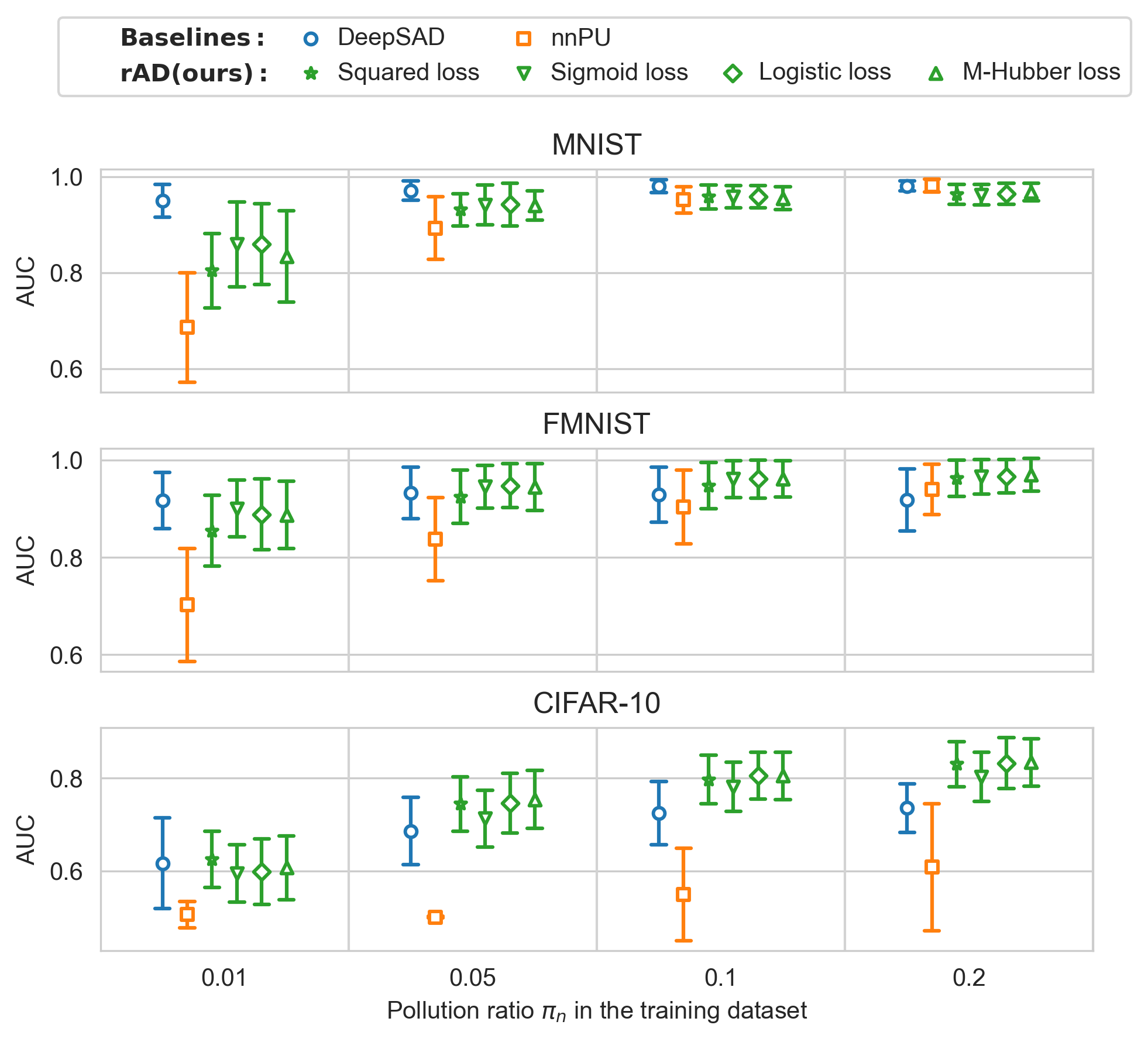
Figure 3: AUC mean and std over 20 trials with various $\pi_{n}$ and default $\gamma_{l}=0.1$

Additional experiments for $\gamma_{l}\in\{0.1,0.2\}$  Figure 3 and Figure 4 respectively report the mean and standard error (std) of the AUC over 20 trials on 3 benchmark datasets with increasing pollution ratio $\pi_{n}$ and $\gamma_{l}=0.1$ and $\gamma_{l}=0.2$.

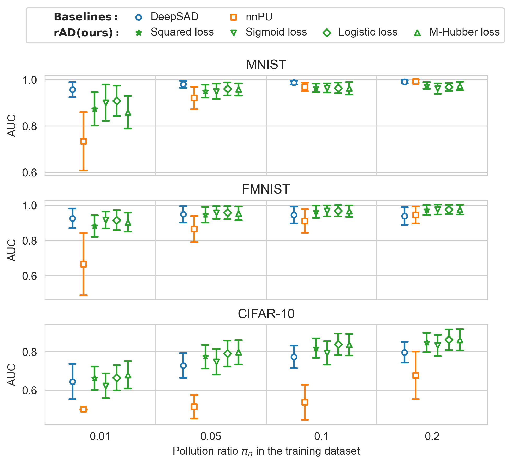
Figure 4: AUC mean and SE over 20 trials with various $\pi_{n}$ and default $\gamma_{l}=0.2$

Impact of $\gamma_{l}$  Figure 5 reports the AUC mean and std over 20 trials at various $\gamma_{l}$ for fixing $\pi_{n}=0.1$.

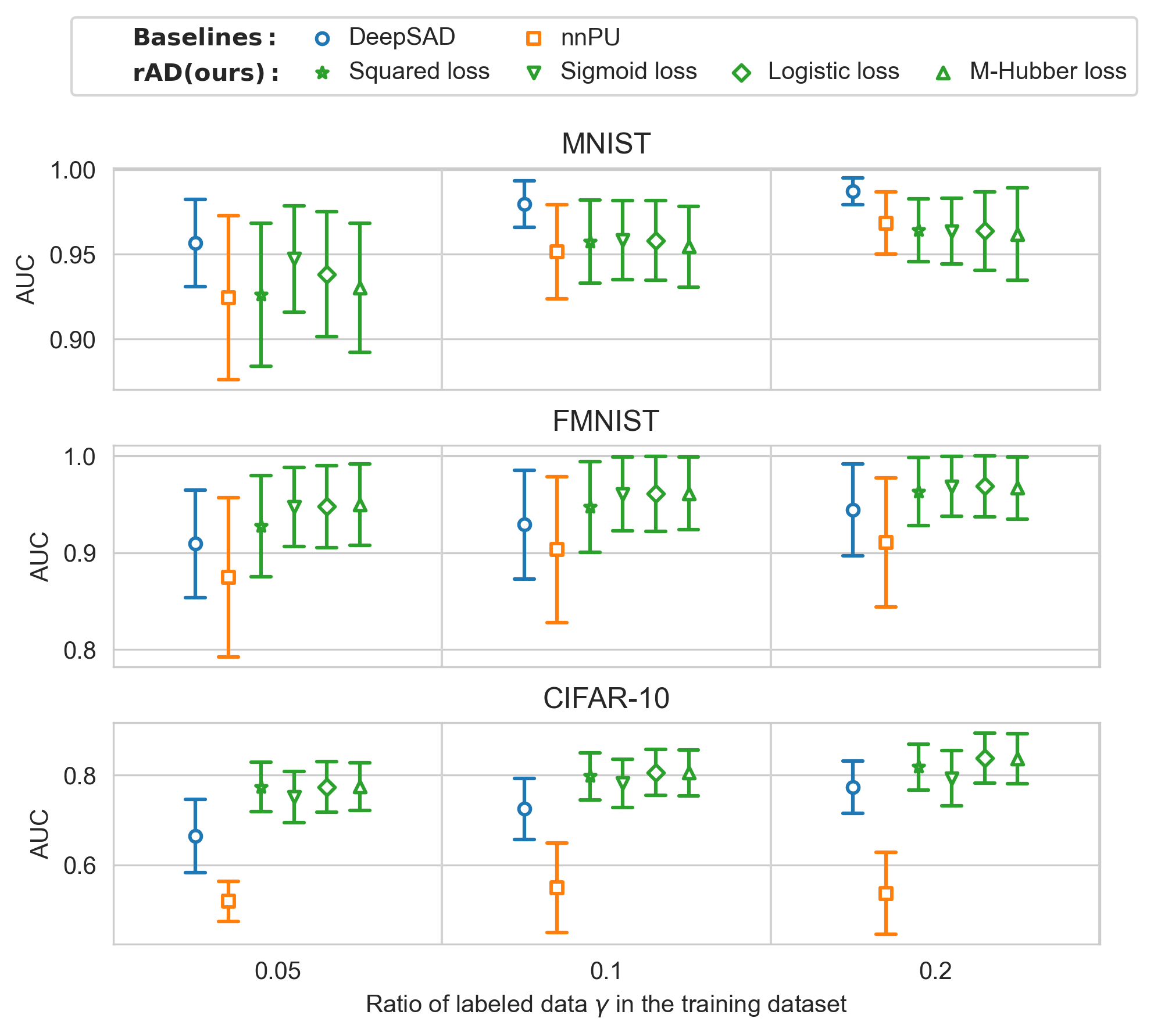
Figure 5: AUC mean and std over 20 trials at various $\gamma_{l}$ for fixing $\pi_{n}=0.1$

Sensitivity analysis for $\pi_{p}^{e}$  Table 6 reports the mean and the standard error of the AUC of deep rAD over the 20 trials for different values of $\pi_{p}^{e}$.

Table 6: AUC means (and standard error) of deep rAD over 20 trials for different $\pi_{p}^{e}$. The significant changes in the AUC means are highlighted in bold.

Dataset Loss $\pi_{p}^{e}=1-\pi_{n}$ $\pi_{p}^{e}=0.9$ $\pi_{p}^{e}=0.8$ $\pi_{p}^{e}=0.7$ $\pi_{p}^{e}=\pi_{n}$ MNIST ($\pi_{n}=0.01$) square 0.66(0.04) 0.70(0.03) 0.72(0.02) 0.68(0.03) 0.65(0.03) sigmoid 0.68(0.03) 0.76(0.03) 0.76(0.03) 0.77(0.03) 0.77(0.03) logistic 0.67(0.03) 0.76(0.03) 0.80(0.03) 0.77(0.03) 0.77(0.03) m-Huber 0.68(0.03) 0.74(0.03) 0.71(0.03) 0.72(0.03) 0.73(0.03) MNIST ($\pi_{n}=0.05$) square 0.85(0.02) 0.87(0.01) 0.89(0.01) 0.89(0.01) 0.86(0.01) sigmoid 0.88(0.01) 0.91(0.01) 0.91(0.01) 0.93(0.01) 0.93(0.01) logistic 0.87(0.02) 0.89(0.01) 0.92(0.01) 0.92(0.01) 0.91(0.01) m-Huber 0.86(0.01) 0.88(0.01) 0.90(0.01) 0.90(0.01) 0.87(0.01) MNIST ($\pi_{n}=0.1$) square 0.92(0.01) 0.92(0.01) 0.93(0.01) 0.93(0.01) 0.89(0.01) sigmoid 0.94(0.01) 0.94(0.01) 0.95(0.01) 0.95(0.01) 0.94(0.01) logistic 0.93(0.01) 0.93(0.01) 0.94(0.01) 0.94(0.01) 0.93(0.01) m-Huber 0.93(0.01) 0.93(0.01) 0.93(0.01) 0.94(0.01) 0.92(0.01) MNIST ($\pi_{n}=0.2$) square 0.95(0.01) 0.95(0.01) 0.95(0.01) 0.96(0.01) 0.94(0.01) sigmoid 0.95(0.01) 0.95(0.01) 0.95(0.01) 0.95(0.01) 0.95(0.01) logistic 0.96(0.01) 0.96(0.01) 0.96(0.01) 0.96(0.01) 0.96(0.01) m-Huber 0.95(0.01) 0.94(0.01) 0.95(0.01) 0.95(0.01) 0.94(0.01) F-MNIST ($\pi_{n}=0.01$) square 0.76(0.02) 0.80(0.01) 0.83(0.02) 0.84(0.02) 0.78(0.02) sigmoid 0.86(0.02) 0.87(0.02) 0.87(0.02) 0.88(0.02) 0.88(0.02) logistic 0.85(0.02) 0.87(0.02) 0.87(0.02) 0.88(0.02) 0.87(0.02) m-Huber 0.82(0.02) 0.88(0.02) 0.87(0.02) 0.87(0.02) 0.83(0.02) F-MNIST ($\pi_{n}=0.05$) square 0.84(0.01) 0.86(0.01) 0.89(0.01) 0.91(0.01) 0.91(0.01) sigmoid 0.93(0.01) 0.93(0.01) 0.93(0.01) 0.94(0.01) 0.95(0.01) logistic 0.91(0.01) 0.92(0.01) 0.93(0.01) 0.93(0.01) 0.95(0.01) m-Huber 0.92(0.01) 0.94(0.01) 0.93(0.01) 0.93(0.01) 0.93(0.01) F-MNIST ($\pi_{n}=0.1$) square 0.88(0.01) 0.88(0.01) 0.93(0.01) 0.94(0.01) 0.94(0.01) sigmoid 0.94(0.01) 0.94(0.01) 0.95(0.01) 0.95(0.01) 0.96(0.01) logistic 0.94(0.01) 0.94(0.01) 0.95(0.01) 0.95(0.01) 0.96(0.01) m-Huber 0.95(0.01) 0.95(0.01) 0.95(0.01) 0.95(0.01) 0.95(0.01) F-MNIST ($\pi_{n}=0.2$) square 0.94(0.01) 0.92(0.01) 0.94(0.01) 0.95(0.01) 0.96(0.01) sigmoid 0.96(0.01) 0.95(0.01) 0.96(0.01) 0.96(0.01) 0.96(0.01) logistic 0.95(0.01) 0.94(0.01) 0.95(0.01) 0.96(0.01) 0.97(0.01) m-Huber 0.96(0.01) 0.94(0.01) 0.96(0.01) 0.96(0.01) 0.96(0.01) CIFAR-10 ($\pi_{n}=0.01$) square 0.60(0.01) 0.60(0.01) 0.59(0.01) 0.60(0.01) 0.59(0.01) sigmoid 0.58(0.01) 0.58(0.02) 0.58(0.02) 0.57(0.02) 0.55(0.02) logistic 0.60(0.02) 0.58(0.02) 0.57(0.02) 0.56(0.02) 0.53(0.02) m-Huber 0.61(0.02) 0.55(0.02) 0.55(0.02) 0.55(0.02) 0.60(0.02) CIFAR-10 ($\pi_{n}=0.05$) square 0.73(0.01) 0.72(0.01) 0.73(0.01) 0.72(0.01) 0.73(0.01) sigmoid 0.66(0.02) 0.68(0.01) 0.69(0.01) 0.67(0.01) 0.69(0.02) logistic 0.71(0.01) 0.71(0.02) 0.71(0.01) 0.70(0.01) 0.69(0.01) m-Huber 0.69(0.01) 0.70(0.01) 0.71(0.01) 0.72(0.01) 0.71(0.01) CIFAR-10 ($\pi_{n}=0.1$) square 0.77(0.01) 0.77(0.01) 0.77(0.01) 0.78(0.01) 0.77(0.01) sigmoid 0.75(0.01) 0.75(0.01) 0.75(0.01) 0.76(0.01) 0.73(0.01) logistic 0.77(0.01) 0.77(0.01) 0.77(0.01) 0.77(0.01) 0.76(0.01) m-Huber 0.77(0.01) 0.77(0.01) 0.77(0.01) 0.78(0.01) 0.77(0.01) CIFAR-10 ($\pi_{n}=0.2$) square 0.80(0.01) 0.80(0.01) 0.80(0.01) 0.80(0.01) 0.80(0.01) sigmoid 0.77(0.01) 0.74(0.01) 0.77(0.01) 0.77(0.01) 0.77(0.01) logistic 0.79(0.01) 0.78(0.01) 0.79(0.01) 0.80(0.01) 0.79(0.01) m-Huber 0.79(0.01) 0.79(0.01) 0.79(0.01) 0.80(0.01) 0.80(0.01)

Sensitivity analysis for $a$  Fixing $\pi_{p}^{e}=0.8$, Figure 6–8 show AUC mean and std of deep rAD with additional values of $a\in\{0.5,0.9\}$ ($a=0.1$ is the default setting) on the datasets with $\gamma_{l}=0.05$ and $\pi_{n}=\in\{0.01,0.05,0.2\}$

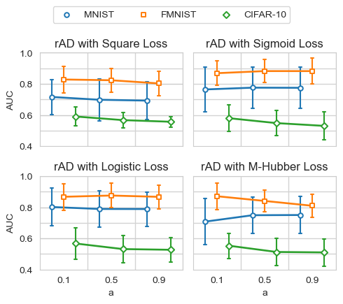
Figure 6: AUC mean and std over 20 trials at various $a$ for the datasets with $\gamma_{l}=0.05$ and $\pi_{n}=0.01$.

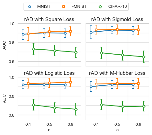
Figure 7: AUC mean and std over 20 trials at various $a$ for the datasets with $\gamma_{l}=0.05$ and $\pi_{n}=0.05$.

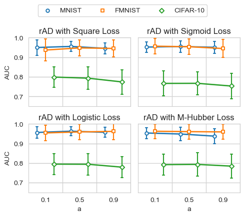
Figure 8: AUC mean and std over 20 trials at various $a$ for the datasets with $\gamma_{l}=0.05$ and $\pi_{n}=0.2$.

ROC curves  Figure 9 shows representative ROC curves obtained by a trial of running the methods (with default settings) on the datasets with $\gamma=0.05$ and $\pi_{n}=0.1$.

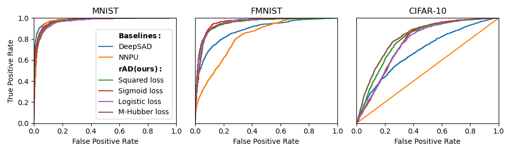
Figure 9: Representative ROC curves for different datasets with $\gamma=0.05$ and $\pi_{n}=0.1$.

References

- Bartlett et al. (2006) Peter L Bartlett, Michael I Jordan, and Jon D McAuliffe. Convexity, classification, and risk bounds. Journal of the American Statistical Association, 101(473):138–156, 2006. doi: 10.1198/016214505000000907.
- Bekker & Davis (2020) Jessa Bekker and Jesse Davis. Learning from positive and unlabeled data: A survey. Machine Learning, 109:719–760, 2020.
- Blanchard et al. (2010) Gilles Blanchard, Gyemin Lee, and Clayton Scott. Semi-supervised novelty detection. Journal of Machine Learning Research, 11(99):2973–3009, 2010. URL http://jmlr.org/papers/v11/blanchard10a.html.
- Chalapathy et al. (2018) Raghavendra Chalapathy, Aditya Menon, and Sanjay Chawla. Anomaly detection using one-class neural networks. 02 2018. http://arxiv.org/abs/1802.06360.
- Chandola et al. (2009) Varun Chandola, Arindam Banerjee, and Vipin Kumar. Anomaly detection. ACM Computing Surveys, 41(3):1–58, 7 2009. ISSN 0360-0300. doi: 10.1145/1541880.1541882. URL https://dl.acm.org/doi/10.1145/1541880.1541882.
- Chaudhari & Shevade (2012) Sneha Chaudhari and Shirish Shevade. Learning from positive and unlabelled examples using maximum margin clustering. In Proceedings of the 19th International Conference on Neural Information Processing - Volume Part III, ICONIP’12, pp. 465–473, Berlin, Heidelberg, 2012. Springer-Verlag. ISBN 9783642344862. doi: 10.1007/978-3-642-34487-9_56. URL https://doi.org/10.1007/978-3-642-34487-9_56.
- Dhillon et al. (2004) Inderjit S. Dhillon, Yuqiang Guan, and Brian Kulis. Kernel k-means: Spectral clustering and normalized cuts. In Proceedings of the Tenth ACM SIGKDD International Conference on Knowledge Discovery and Data Mining, KDD ’04, pp. 551–556, New York, NY, USA, 2004. Association for Computing Machinery. ISBN 1581138881. doi: 10.1145/1014052.1014118. URL https://doi.org/10.1145/1014052.1014118.
- du Plessis & Sugiyama (2013) Marthinus du Plessis and Masashi Sugiyama. Semi-supervised learning of class balance under class-prior change by distribution matching. Neural networks : the official journal of the International Neural Network Society, 50C:110–119, 11 2013. doi: 10.1016/j.neunet.2013.11.010.
- du Plessis et al. (2014) Marthinus C du Plessis, Gang Niu, and Masashi Sugiyama. Analysis of learning from positive and unlabeled data. In Z. Ghahramani, M. Welling, C. Cortes, N. Lawrence, and K.Q. Weinberger (eds.), Advances in Neural Information Processing Systems, volume 27. Curran Associates, Inc., 2014. URL https://proceedings.neurips.cc/paper/2014/file/35051070e572e47d2c26c241ab88307f-Paper.pdf.
- du Plessis et al. (2015) Marthinus C du Plessis, Gang Niu, and Masashi Sugiyama. Convex formulation for learning from positive and unlabeled data. In Francis Bach and David Blei (eds.), Proceedings of the 32nd International Conference on Machine Learning, volume 37 of Proceedings of Machine Learning Research, pp. 1386–1394, Lille, France, 07–09 Jul 2015. PMLR. URL https://proceedings.mlr.press/v37/plessis15.html.
- Elkan & Noto (2008) Charles Elkan and Keith Noto. Learning classifiers from only positive and unlabeled data. In Proceedings of the 14th ACM SIGKDD International Conference on Knowledge Discovery and Data Mining, KDD ’08, pp. 213–220, New York, NY, USA, 2008. Association for Computing Machinery. ISBN 9781605581934. doi: 10.1145/1401890.1401920. URL https://doi.org/10.1145/1401890.1401920.
- Erfani et al. (2016) Sarah M. Erfani, Sutharshan Rajasegarar, Shanika Karunasekera, and Christopher Leckie. High-dimensional and large-scale anomaly detection using a linear one-class SVM with deep learning. Pattern Recognition, 58:121–134, 10 2016. ISSN 0031-3203. doi: 10.1016/J.PATCOG.2016.03.028.
- Görnitz et al. (2009) Nico Görnitz, Marius Kloft, and Ulf Brefeld. Active and semi-supervised data domain description. In Lect Notes Artif Intell., volume 5781, pp. 407–422, 09 2009. ISBN 978-3-642-04179-2. doi: 10.1007/978-3-642-04180-8_44.
- Görnitz et al. (2013) Nico Görnitz, Marius Kloft, Konrad Rieck, and Ulf Brefeld. Toward supervised anomaly detection. Journal of Artificial Intelligence Research, 46:235–262, 2013.
- Görnitz et al. (2018) Nico Görnitz, Luiz Alberto Lima, Klaus-Robert Müller, Marius Kloft, and Shinichi Nakajima. Support vector data descriptions and -means clustering: One class? IEEE Transactions on Neural Networks and Learning Systems, 29(9):3994–4006, 2018. doi: 10.1109/TNNLS.2017.2737941.
- Han et al. (2022) Songqiao Han, Xiyang Hu, Hailiang Huang, Mingqi Jiang, and Yue Zhao. Adbench: Anomaly detection benchmark. In Neural Information Processing Systems (NeurIPS), 2022.
- Hawkins (1974) Douglas M. Hawkins. The detection of errors in multivariate data using principal components. Journal of the American Statistical Association, 69(346):340–344, 1974. ISSN 01621459.
- Hawkins et al. (2002) Simon Hawkins, Hongxing He, Graham Williams, and Rohan Baxter. Outlier detection using replicator neural networks. In Yahiko Kambayashi, Werner Winiwarter, and Masatoshi Arikawa (eds.), Data Warehousing and Knowledge Discovery, pp. 170–180, Berlin, Heidelberg, 2002. Springer Berlin Heidelberg. ISBN 978-3-540-46145-6.
- Hodge & Austin (2004) Victoria Hodge and Jim Austin. A survey of outlier detection methodologies. Artificial Intelligence Review, 22:85–126, 10 2004. doi: 10.1023/B:AIRE.0000045502.10941.a9.
- Hsieh et al. (2019) Yu-Guan Hsieh, Gang Niu, and Masashi Sugiyama. Classification from positive, unlabeled and biased negative data. In Kamalika Chaudhuri and Ruslan Salakhutdinov (eds.), Proceedings of the 36th International Conference on Machine Learning, volume 97 of Proceedings of Machine Learning Research, pp. 2820–2829. PMLR, 09–15 Jun 2019.
- Huang et al. (2006) Ling Huang, XuanLong Nguyen, Minos Garofalakis, Michael Jordan, Anthony Joseph, and Nina Taft. In-network pca and anomaly detection. In B. Schölkopf, J. Platt, and T. Hoffman (eds.), Advances in Neural Information Processing Systems, volume 19. MIT Press, 2006. URL https://proceedings.neurips.cc/paper/2006/file/2227d753dc18505031869d44673728e2-Paper.pdf.
- Ju et al. (2020) Hyunjun Ju, Dongha Lee, Junyoung Hwang, Junghyun Namkung, and Hwanjo Yu. Pumad: Pu metric learning for anomaly detection. Information Sciences, 523:167–183, 2020. ISSN 0020-0255. doi: https://doi.org/10.1016/j.ins.2020.03.021. URL https://www.sciencedirect.com/science/article/pii/S0020025520302012.
- Khan & Madden (2014) Shehroz S. Khan and Michael G. Madden. One-class classification: taxonomy of study and review of techniques. The Knowledge Engineering Review, 29(3):345–374, 2014. doi: 10.1017/S026988891300043X.
- Kiran et al. (2018) Bangalore Kiran, Dilip Thomas, and Ranjith Parakkal. An overview of deep learning based methods for unsupervised and semi-supervised anomaly detection in videos. Journal of Imaging, 4, 01 2018. doi: 10.3390/jimaging4020036.
- Kiryo et al. (2017) Ryuichi Kiryo, Gang Niu, Marthinus D du Plessis, and Masashi Sugiyama. Positive-unlabeled learning with non-negative risk estimator. In I. Guyon, U. Von Luxburg, S. Bengio, H. Wallach, R. Fergus, S. Vishwanathan, and R. Garnett (eds.), Advances in Neural Information Processing Systems, volume 30. Curran Associates, Inc., 2017. URL https://proceedings.neurips.cc/paper/2017/file/7cce53cf90577442771720a370c3c723-Paper.pdf.
- Lecun et al. (2006) Yann Lecun, Sumit Chopra, and Raia Hadsell. A tutorial on energy-based learning. MIT Press, 01 2006.
- Ledoux & Talagrand (1991) Michel Ledoux and Michel Talagrand. Probability in Banach Spaces: Isoperimetry and Processes. Springer Berlin Heidelberg, Berlin, Heidelberg, 1991. ISBN 978-3-642-20212-4. doi: 10.1007/978-3-642-20212-4_6. URL https://doi.org/10.1007/978-3-642-20212-4_6.
- Lee & Liu (2003) Wee Sun Lee and Bing Liu. Learning with positive and unlabeled examples using weighted logistic regression. In Proceedings of the Twentieth International Conference on International Conference on Machine Learning, ICML’03, pp. 448–455. AAAI Press, 2003. ISBN 1577351894.
- Li et al. (2019) Dan Li, Dacheng Chen, Lei Shi, Baihong Jin, Jonathan Goh, and See-Kiong Ng. Mad-gan: Multivariate anomaly detection for time series data with generative adversarial networks. In International Conference on Artificial Neural Networks, 2019.
- Li & Liu (2003) Xiaoli Li and Bing Liu. Learning to classify texts using positive and unlabeled data. In Proceedings of Eighteenth International Joint Conference on Artificial Intelligence (IJCAI-03): 2003; Acapulco, Mexico, pp. 587–594, 01 2003.
- Liu et al. (2003) B. Liu, Y. Dai, X. Li, W.S. Lee, and P.S. Yu. Building text classifiers using positive and unlabeled examples. In Third IEEE International Conference on Data Mining, pp. 179–186, 2003. doi: 10.1109/ICDM.2003.1250918.
- McDiarmid (1989) Colin McDiarmid. On the method of bounded differences. In Surveys in Combinatorics, 1989.
- Mohri et al. (2018) Mehryar Mohri, Afshin Rostamizadeh, and Ameet Talwalkar. Foundations of Machine Learning. Adaptive Computation and Machine Learning. MIT Press, Cambridge, MA, 2 edition, 2018. ISBN 978-0-262-03940-6.
- Munoz-Mari et al. (2010) Jordi Munoz-Mari, Francesca Bovolo, Luis Gomez-Chova, Lorenzo Bruzzone, and Gustavo Camp-Valls. Semisupervised one-class support vector machines for classification of remote sensing data. IEEE Transactions on Geoscience and Remote Sensing, 48(8):3188–3197, 2010. doi: 10.1109/TGRS.2010.2045764.
- Niu et al. (2016) Gang Niu, Marthinus C. du Plessis, Tomoya Sakai, Yao Ma, and Masashi Sugiyama. Theoretical comparisons of positive-unlabeled learning against positive-negative learning. In NIPS’16, pp. 1207–1215, Red Hook, NY, USA, 2016. Curran Associates Inc. ISBN 9781510838819.
- Pang et al. (2020) Guansong Pang, Chunhua Shen, Longbing Cao, and Anton van den Hengel. Deep Learning for Anomaly Detection: A Review. ACM Computing Surveys, 54(2), 7 2020. doi: 10.1145/3439950. URL http://arxiv.org/abs/2007.02500http://dx.doi.org/10.1145/3439950.
- Parzen (1962) Emanuel Parzen. On Estimation of a Probability Density Function and Mode on JSTOR. The annals of mathematical statistics, 33(3):1065–1076, 1962.
- Pimentel et al. (2014) Marco A.F. Pimentel, David A. Clifton, Lei Clifton, and Lionel Tarassenko. A review of novelty detection. Signal Processing, 99:215–249, 2014. ISSN 0165-1684. doi: https://doi.org/10.1016/j.sigpro.2013.12.026. URL https://www.sciencedirect.com/science/article/pii/S016516841300515X.
- Pincus (1995) R. Pincus. Barnett, v., and lewis t.: Outliers in statistical data. 3rd edition. j. wiley & sons 1994, xvii. 582 pp., £49.95. Biometrical Journal, 37(2):256–256, 1995. doi: https://doi.org/10.1002/bimj.4710370219. URL https://onlinelibrary.wiley.com/doi/abs/10.1002/bimj.4710370219.
- Rousseeuw (1985) Peter J Rousseeuw. Multivariate estimation with high breakdown point. Mathematical statistics and applications, 8(37):283–297, 1985.
- Rousseeuw & Van Driessen (1999) Peter J. Rousseeuw and Katrien Van Driessen. A fast algorithm for the minimum covariance determinant estimator. Technometrics, 41(3):212–223, 1999. ISSN 15372723. doi: 10.1080/00401706.1999.10485670. URL https://www.tandfonline.com/action/journalInformation?journalCode=utch20.
- Ruff et al. (2018) Lukas Ruff, Robert Vandermeulen, Nico Goernitz, Lucas Deecke, Shoaib Ahmed Siddiqui, Alexander Binder, Emmanuel Müller, and Marius Kloft. Deep one-class classification. In Jennifer Dy and Andreas Krause (eds.), Proceedings of the 35th International Conference on Machine Learning, volume 80 of Proceedings of Machine Learning Research, pp. 4393–4402. PMLR, 10–15 Jul 2018.
- Ruff et al. (2020) Lukas Ruff, Robert A. Vandermeulen, Nico Görnitz, Alexander Binder, Emmanuel Müller, Klaus-Robert Müller, and Marius Kloft. Deep semi-supervised anomaly detection. In International Conference on Learning Representations, 2020. URL https://openreview.net/forum?id=HkgH0TEYwH.
- Ruff et al. (2021) Lukas Ruff, Jacob Kauffmann, Robert Vandermeulen, Gregoire Montavon, Wojciech Samek, Marius Kloft, Thomas Dietterich, and Klaus-Robert Müller. A unifying review of deep and shallow anomaly detection. Proceedings of the IEEE, PP:1–40, 02 2021. doi: 10.1109/JPROC.2021.3052449.
- Saerens et al. (2002) Marco Saerens, Patrice Latinne, and Christine Decaestecker. Adjusting the outputs of a classifier to new a priori probabilities: A simple procedure. Neural computation, 14:21–41, 02 2002. doi: 10.1162/089976602753284446.
- Sakai et al. (2017) Tomoya Sakai, Marthinus Christoffel du Plessis, Gang Niu, and Masashi Sugiyama. Semi-supervised classification based on classification from positive and unlabeled data. In Doina Precup and Yee Whye Teh (eds.), Proceedings of the 34th International Conference on Machine Learning, volume 70 of Proceedings of Machine Learning Research, pp. 2998–3006. PMLR, 06–11 Aug 2017. URL https://proceedings.mlr.press/v70/sakai17a.html.
- Schölkopf et al. (2001) Bernhard Schölkopf, John Platt, John Shawe-Taylor, Alexander Smola, and Robert Williamson. Estimating support of a high-dimensional distribution. Neural Computation, 13:1443–1471, 07 2001. doi: 10.1162/089976601750264965.
- Tax & Duin (1999) David M.J. Tax and Robert P.W. Duin. Support vector domain description. Pattern Recognition Letters, 20(11-13):1191–1199, 11 1999. ISSN 0167-8655. doi: 10.1016/S0167-8655(99)00087-2.
- Tax & Duin (2004) David M.J. Tax and Robert P.W. Duin. Support vector data description. Machine Learning, 54:45–66, 2004. doi: 10.1023/B:MACH.0000008084.60811.49.
- Wang & Cherian (2019) Jue Wang and Anoop Cherian. Gods: Generalized one-class discriminative subspaces for anomaly detection. In 2019 IEEE/CVF International Conference on Computer Vision (ICCV), pp. 8200–8210, 2019. doi: 10.1109/ICCV.2019.00829.
- Yan et al. (2021) Xudong Yan, Huaidong Zhang, Xuemiao Xu, Xiaowei Hu, and Pheng-Ann Heng. Learning Semantic Context from Normal Samples for Unsupervised Anomaly Detection. Proceedings of the AAAI Conference on Artificial Intelligence, 35(4):3110–3118, 5 2021. URL https://ojs.aaai.org/index.php/AAAI/article/view/16420.
- Zimek et al. (2012) Arthur Zimek, Erich Schubert, and Peer Kröger. A survey on unsupervised outlier detection in high-dimensional numerical data. Statistical Analysis and Data Mining, 5:363–387, 10 2012. doi: 10.1002/sam.11161.