Interpreting Sentiment Composition with Latent Semantic Tree

Abstract

As the key to sentiment analysis, sentiment composition considers the classification of a constituent via classifications of its contained sub-constituents and rules operated on them. Such compositionality has been widely studied previously in the form of hierarchical trees including untagged and sentiment ones, which are intrinsically suboptimal in our view. To address this, we propose semantic tree, a new tree form capable of interpreting the sentiment composition in a principled way. Semantic tree is a derivation of a context-free grammar (CFG) describing the specific composition rules on difference semantic roles, which is designed carefully following previous linguistic conclusions. However, semantic tree is a latent variable since there is no its annotation in regular datasets. Thus, in our method, it is marginalized out via inside algorithm and learned to optimize the classification performance. Quantitative and qualitative results demonstrate that our method not only achieves better or competitive results compared to baselines in the setting of regular and domain adaptation classification, and also generates plausible tree explanations.

1 Introduction

Sentiment classification is a task to determine the sentiment polarity of a sentence Yadav and Vishwakarma (2020); Dang et al. (2020). Current researches on this task are gradually shifting from improving model performance to interpretability. As the most known stream, feature-based explanation tries to figure out which input feature, say word, has the most influence on the prediction, in the form of the salience score or rationale, and in both self and post-hoc settings Li et al. (2016); Ribeiro et al. (2016); Kim et al. (2020); Lei et al. (2016); Bastings et al. (2019); De Cao et al. (2020). However, this task requires sentiment composition Polanyi and Zaenen (2006), which is beyond the ability of these feature-based explanations.

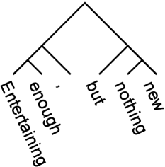
(a) Untagged tree.

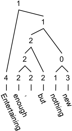
(b) Sentiment tree.

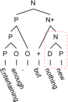
(c) Semantic tree.

Figure 1: Different tree structures for explanining sentiment composition, where semantic tree can explain the sentiment composition in the inverted-V structure, as shown in the box of (c).

To be concrete, sentiment composition considers the classification of a constituent via 1) classifications of its contained sub-constituents and 2) rules operated on them Moilanen and Pulman (2007), as shown in Figure 1(c). Thus, the classification of a sentence is decomposed into hierarchical sentiment compositions of its sub-constituents. Such compositionality has been widely studied previously in the form of hierarchical trees including untagged tree and sentiment tree, as shown in Figure 1. Untagged tree is usually modeled as a latent variable and learned via the task objective Yogatama et al. (2017); Maillard and Clark (2018); Choi et al. (2018); Havrylov et al. (2019); Chowdhury and Caragea (2021). Then, a TreeLSTM Tai et al. (2015); Zhu et al. (2015) is adopted to encode the sentence following the hierarchy for the final prediction. However, untagged tree is limited because it can only explain the hierarchy but not give labels on all nodes. Sentiment tree takes a further step that every node within has a polarity score or label. As the most representative example, Socher et al. (2013) creates Stanford Sentiment Treebank (SST) that has sentiment tree annotation. Sentiment tree also appears as a post-hoc explanation giving hierarchical attribution scores Chen et al. (2020); Zhang et al. (2020). However, in fact, not every constituent is sentimental, some of which are somewhat more functional. For example, while a negator “not" is sentimentally neural, it can functionally flip the sentiment of a constituent. Sentiment labels are therefore not sufficient to explain such phenomenon.

To overcome those defects, we propose semantic tree, a new tree form capable of explicitly and principally interpreting the sentiment composition. In the semantic tree, each node is assigned a label in semantic labels including sentimental and functional ones, and each local inverted-V structure reveals the rule composing adjacent constituents, as shown in Figure 1(c). Inspired by Dong et al. (2015), formally, the semantic tree is a derivation of a context-free grammar (CFG) Chomsky (1956) defined by non-terminal symbols (semantic labels), terminal symbols (word vocabulary), rules, and root symbols (positive and negative). The challenge of designing such grammar lies in designing semantic labels and rules, which requires linguistic knowledge of sentiment composition. To address this, we follow previous work about sentiment composition Polanyi and Zaenen (2006); Moilanen and Pulman (2007); Taboada et al. (2011) to carefully design 11 semantic labels and 62 rules. We believe the grammar could cover most cases in sentiment analysis, as shown in Table 1.

We aim to learn a model capable of extracting the semantic tree using data consisting of only sentence-label pairs, which is challenging because the semantic tree is latent without full annotation. To address this, we first build a semantic tree parser, and then marginalize out the semantic tree to induce a sentiment classifier to conduct supervised training on such data. Fortunately, this marginalization over the exponential tree space is computationally tractable resorting to the inside algorithm Baker (1979). This process could be abstracted as a module, namely sentiment composition module (SCM), which computes the compatibility of a prediction in the view of sentiment composition but not only pattern recognition. Accompanying an arbitrary neural text encoder with the proposed SCM, we can build a self-explanatory model that can not only predict the sentiment label but also generate a semantic tree as the explanation. To learn more plausible semantic trees, we further propose two extra objectives to guide the preterminals in the semantic tree, and to make the tree structure more syntactically meaningful.

We conduct experiments on three datasets including MR Pang and Lee (2005), SST2 Socher et al. (2013) and Amazon Blitzer et al. (2007) in the setting of regular and cross-domain classification. Quantitative and qualitative results demonstrate that our method not only achieves better or competitive results compared to baselines, and also generates plausible tree explanations.

2 Method

2.1 Problem Formalization

The dataset is a collection of tuples $\{(x^{n},y^{n})\}_{n=1}^{N}$, each of which contains a sentence $x\in\cal{V}^{*}$ and a sentiment label $y\in\cal{Y}$, where $\cal{V}$ is the word vocabulary and ${\cal Y}=\{P,N\}$ is the label set consisting of positive ($P$) and negative ($N$). The task goal is to learn a classifier $p(y|x)$. Since we hope to generate a semantic tree of the input sentence where the sentiment label is its root label, as shown in Figure 1(c), the objective classifier $p(y|x)$ is not directly parameterized by a discriminative model as usual. Instead, we define the classifier as the marginalization of a parser over the latent semantic tree, in which the parser could fulfill this purpose. Concretely, let ${\cal T}_{x}(y)$ be the set of all semantic trees rooted $y$. Naturally, we have:

$$p(y|x)=\sum_{t\in{\cal T}_{x}(y)}p(t|x)$$ (1)

where $p(t|x)$ is a semantic tree parser that accepts a sentence and generates a semantic tree. We can conduct supervised learning when the classifier $p(y|x)$ is obtained, where the parser $p(t|x)$ is implicitly learned in this process. After training, the model can do the prediction via the induced classifier $p(y|x)$, and generate the semantic tree to real the sentiment composition process of it.

The very first issue before solving the summation in Equation (1) is to formalize the semantic tree. For simplicity, we can assume that the label of a constituent is determined immediately by its sub-constituents, regardless of the surrounding context. Therefore, the semantic tree is viewed as a derivation of a CFG that defines specific semantic labels and composition rules. Now, two challenges remain: 1) How to properly define the CFG behind the semantic tree? 2) How to model the parser $p(t|x)$ and efficiently compute the classifier $p(y|x)$? We shall elaborate these two problems in Section 2.2 and Section 2.3, respectively.

2.2 Sentiment Composition Grammar

The proposed semantic tree is described by a context-free grammar ${\cal G}$ consisting a quadruple including the non-terminal symbol set ${\cal N}$ (semantic label set), the terminal symbol set ${\cal V}$ (word vocabulary), the composition rule set ${\cal R}$ and the root symbol set ${\cal Y}$ ($P$ and $N$). While ${\cal V}$ and ${\cal Y}$ are obvious, the design of semantic labels (${\cal N}$) and composition rules (${\cal R}$) requires expert knowledge. Fortunately, previous works have concluded different types of compositions exhaustively Polanyi and Zaenen (2006); Moilanen and Pulman (2007); Taboada et al. (2011), inspiring us to design 11 semantic labels and 62 composition rules. We call the proposed grammar as a sentiment composition grammar (SCG).

Semantic Labels

The defined 11 semantic labels include two types as follows:

Sentimental labels

Including negative $N$, positive $P$, neutral $O$.

Functional labels

Including negator $D$, irrealis blocker $I$, priority riser $+$, priority reducer $-$, high negative $N^{+}$, high positive $P^{+}$, low negative $N^{-}$, low positive $P^{-}$.

We shall explain these labels together with composition rules later.

Composition Rules

Formally, the composition rule is in the form of $\beta\rightarrow A$ ($A\in{\cal N}$, $\beta\in({\cal N}\cup{\cal V})^{*}$), which determines the label of a constituent given its sub-constituents. We include three types of rules.

The first one is binary rule in the form of $BC\rightarrow A$ ($A,B,C\in{\cal N}$). Binary rules are defined following common binary compositions, which mainly includes four types according to previous works and our observations. We now introduce each composition and its corresponding rules.

Polarity propagation

Propagating the polarity:

$$N\ O/N\rightarrow N,\ P\ O/P\rightarrow P,\ O\ O\rightarrow O$$ (2)

Negation

Flipping the non-neutral polarity ($P/N$) via a negator ($D$):

$$D\ P\rightarrow N,D\ N\rightarrow P$$ (3)

Conflict Resolution

Resolving the conflict of non-neutral polarity constituents ($P/N$) by ranking their priorities based on priority modifiers ($+/-$). As a typical example, Figure 1 shows a contrastive conjunction Socher et al. (2013) structure, which the first and the second half of the sentence have opposite polarities. The connector “but” is a priority riser ($+$) that rises the priority of the second half sentence, which dominates the entire sentence priority. Similarly, there also exist priority reducer ($-$) such as “although”. Thus, rules related to this composition includes those for priority modification:

$$+\ P\rightarrow P^{+},-\ P\rightarrow P^{-}$$ (4)

and those for resolution:

$$N\ P^{+}\rightarrow P,N^{-}\ P^{+}\rightarrow P$$ (5)

We don’t allow the polarity with priority ($N^{+}/N^{-}/P^{+}/P^{-}$) without a explicit modifier $+/-$, which a single word with non-neutral polarity can’t have priority.

Irrealis blocking

Neutralizing the non-neutral polarity ($P/N$) by an irrealis blocker $(I)$:

$$I\ P/N\rightarrow O$$ (6)

The blocker such as modal “would” or connector “if” can set up a context about possibility of some polarities not necessarily expressed by the author. As a result, a literal polarity is canceled.

The full binary rule list is shown in Table 6 in Appendix A. We also present examples of those compositions Figure 2. Those compositions appears very commonly. To illustrate this, we randomly sample 100 examples in SST2 and MR and count occurrences of above compositions, where 97 and 98 examples in SST2 and MR can be explained by the above compositions. Thus, we believe our rules can cover most cases.

The second type is terminal-unary rule defining the legal preterminals of single words, which is in the form of $\omega\rightarrow A$ ($A\in{\cal N}_{\rm pret}=\{N,P,O,D,I,+,-\},\omega\in{\cal V}$). As introduced, $A$ can’t be the polarity priority ($N^{+}/N^{-}/P^{+}/P^{-}$).

We further define the preterminal-unary rule as the third type, including rules $A\rightarrow A$ ($A\in\{P,N,O,D,I,+,-\}$) and $D/I/+/-\rightarrow O$. Those rules can only and must appear on the second layer of the semantic tree, which is designed to cancel the function of misrecognized function constituents, leading to better performance in our experiments.

(a) Polarity propagation.

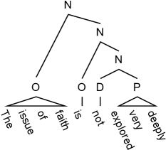
(b) Negation.

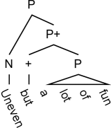
(c) Conflict resolution.

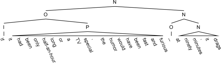
(d) Irrealis blocking.

Figure 2: Examples of different binary compositions.

Composition	SST2	MR
Polarity propagation	97	96
Negation	18	18
Conflict resolution	18	20
Irrealis blocking	6	9
None of the above	3	4

Table 1: The number of existences in the sampled 100 sentences in SST2 and MR.

2.3 Sentiment Composition Module

We now answer the second question: How to model the parser $p(t|x)$ and compute the classifier $p(y|x)$. We show that this process naturally lead to the sentiment composition module.

Semantic Tree Parser

First, we represent the semantic tree $t$ of a sentence $x=(x_{0},\cdots,x_{T-1})$ by the set of anchored rules Eisner (2016) consisting of a rule and its location indices:

$$t=\{(B_{ik}C_{kj}\rightarrow A_{ij})_{t}|1\leq t\leq T-1\}$$ (7)

$$\cup\{(B_{i}\rightarrow A_{i})_{t}|1\leq t\leq T\}$$

$$\cup\{(x_{i}\rightarrow A_{i})_{t}|1\leq t\leq T\}$$

where $A_{ij}\ (0\leq i<j<T)$ is an anchored node suggesting a label $A$ covering the constituent ranging from $x_{i}$ to $x_{j-1}$. $A_{i}$ is short for $A_{i,i+1}$ which is an unary anchored node covering the word $x_{i}$. Thus, $B_{ik}C_{kj}\rightarrow A_{ij}$, $B_{i}\rightarrow A_{i}$ and $x_{i}\rightarrow A_{i}$ represent the binary, preterminal-unary, and terminal-unary anchroed rule, respectively.

The semantic tree parser $p(t|x)$ is defined by a Gibbs distribution on anchored rules in a tree Finkel et al. (2008); Durrett and Klein (2015):

$$p(t|x)=\frac{1}{Z(x)}\prod_{a\in t}\phi(a)=\frac{1}{Z(x)}\exp\left(\sum_{a\in t}s(a)\right)$$ (8)

where $Z(x)$ is the log-partition function for normalization. $\phi(a)>0$ is the potential function of the anchored rule $a$ defined in the exponential form $\exp(s(a))$, where $s(a)$ is the score to rate how comfortable it is for $a$ to appear in the tree. Scores for different types of anchored rules are defined as the sum of a few subscores rating the comfortableness of corresponding substructures.

$$s(B_{ik}C_{kj}\rightarrow A_{ij})=$$ (9)

$$\qquad s_{\rm rule}(BC\rightarrow A)+s_{\rm label}(A,x_{ij})+s_{\rm span}(x_{ij})$$

$$s(B_{i}\rightarrow A_{i})=$$

$$\qquad s_{\rm rule}(B\rightarrow A)+s_{\rm label}(A,x_{i})+s_{\rm span}(x_{i})$$

$$s(x_{i}\rightarrow A_{i})=s_{\rm rule}(x_{i}\rightarrow A)$$

Here the scores of binary and pos-unary rules $s_{\rm rule}(BC\rightarrow A)$ and $s_{\rm rule}(B\rightarrow A)$ are scalar parameters. Other scores are modeled by neural networks:

$$s_{\rm rule}(x_{i}\rightarrow A)={\bf w}_{\rm rule}^{A}\cdot{\bf h}_{i}^{\leq L}+b_{\rm rule}^{A}$$ (10)

$$s_{\rm label}(A,x_{ij})={\bf w}_{\rm label}^{A}\cdot{\bf h}_{ij}^{L}+b_{\rm label}^{A}$$

$$s_{\rm span}(x_{ij})={\bf w}_{\rm span}\cdot{\bf h}_{ij}^{L}+b_{\rm span}$$

where $\cdot$ is the vector dot product. ${\bf w}_{\cdot}^{\cdot}$ and $b_{\cdot}^{\cdot}$ are learning parameters. ${\bf h}_{ij}^{l}$ is the phrase representation of the constituent $x_{ij}$ in the $l$ layer, which is computed by a text encoder $m$:

$${\bf h}_{0}^{0},\cdots,{\bf h}_{T-1}^{0},\cdots,{\bf h}_{0}^{L-1},\cdots,{\bf h}_{T-1}^{L-1}$$ (11)

$$\qquad\qquad=m({\bf e}_{0},\cdots,{\bf e}_{T-1})$$

$${\bf h}_{ij}^{l}=\frac{\sum_{t=i}^{j-1}{\bf h}_{t}^{l}}{j-i}$$

where ${\bf e}_{i}$ is the word embedding of $x_{i}$. Note that we compute $s_{\rm label}$ and $s_{\rm span}$ using top layer phrase representations, but compute $s_{\rm rule}$ using a lower layer one. This is because the recognition of the preterminal is easier than determining if this label is cancelled. Thus the simple phrase representation ${\bf h}_{ij}^{\leq L}$ is sufficient for the former, while the more “contextual” one ${\bf h}_{ij}^{L}$ is in favor by the latter.

Inducing the Classifier from the Parser

As shown in Equation (1), the classifier is induced by marginalizing over all the semantic trees of the input sentence, which can be efficient done by the inside algorithm. To illustrate this, we first let ${\cal T}_{x}(A_{ij})$ and ${\cal T}_{x}(B_{ik}C_{kj}\rightarrow A_{ij})$ be sets of subtrees of sentence $x$ that are covered by the anchored node $A_{ij}$ and rule $B_{ik}C_{kj}\rightarrow A_{ij}$, respectively. The inside algorithm defines the inside term $\alpha_{x}(A_{ij})=\sum_{t\in{\cal T}_{x}(A_{ij})}\prod_{a\in t}\phi(a)$, which is the sum of the potentials of subtrees covered by $A_{ij}$. The inside term is computed recursively in a bottom-up manner:

$$\alpha_{x}( A_{i})=\phi(x_{i}\rightarrow A_{i})\sum_{B\rightarrow A\in{\cal R}}\phi(B_{i}\rightarrow A_{i})$$ (12)

$$\alpha_{x}( A_{ij})=$$

$$\sum_{BC\rightarrow A\in{\cal R}\atop i<k<j}\phi(B_{ik}C_{kj}\rightarrow A_{ij})\alpha_{x}({B_{ik}})\alpha_{x}(C_{kj})$$

where $\alpha_{x}(A_{i})$ is the initial value of this recursion. Obvious, the time complexity of the inside algorithm is $O(|{\cal R}|T^{3})$. It can be shown that the inside term of the root anchored node $\alpha_{x}(A_{0T})$, abbreviated as $\alpha_{x}(A)$, equals to the unnormalized probability that the root of the semantic tree is $y$. Thus, we have:

$$p(y=A|x)=\frac{\alpha_{x}(A)}{\sum_{B\in{\cal Y}}\alpha_{x}(B)}$$ (13)

$$\qquad=\frac{\exp(s_{\rm label}(A,x)+s_{\rm SCM}(A,x))}{\sum_{B\in{\cal Y}}\exp(s_{\rm label}(B,x)+s_{\rm SCM}(B,x))}$$

$$s_{\rm SCM}(A,x)=\mathop{\rm logsumexp}_{BC\rightarrow A\in{\cal R}\atop 0<k<T}\left(s_{\rm rule}(BC\rightarrow A)\right.$$

$$\qquad\qquad\qquad\left.+\log\alpha_{x}(B_{0k})+\log\alpha_{x}(C_{kT})\right)$$

As seen, the logit in the softmax includes an extra score $s_{\rm SCM}(A,x)$ as a complement to the regular one $s_{\rm label}(A,x)$, where the former and the latter can be understood as the accordance of assigning the label $A$ by means of sentiment composition and pattern recognition, respectively. Thus, we call $s_{\rm label}$ and $s_{\rm SCM}$ as the recognition module and the sentiment composition module, respectively. While the recognition module is only learned from the data, the sentiment composition module incorporates general and invariant human knowledge in the form of sentiment composition rules, which is more robust for domain adaptation, as we shall see in Section 4.1.

The last issue is that the proposed SCM is intractable for long documents due to the cube time complexity over length. So for a document, we first cut it into sentences, and then compute their individual logits. Document logits are aggregated by attention on those sentence logits, where attention weights are computed by sentence representations.

2.4 Training & Testing

Now we’ve obtained the induced classifier, we can apply supervised training by minimizing:

$${\cal L}_{\rm cls}=-\frac{1}{N}\sum_{n=1}^{N}\log p(y^{n}|x^{n})$$ (14)

This objective might be enough for the classification, but not for a plausible semantic tree explanation. Cases in which a semantic tree can reach a right root label with wrong preterminals and improper structure do exist. For example, if we choose BERT Devlin et al. (2019) as the encoder, the method might assign non-neutral polarity to [CLS], and recognize any other tokens as neutral polarity, since [CLS] representation is usually treated as the sentence representation. An effective way to improve the plausibility is to learn the explanation via more explicit annotations Strout et al. (2019); Zhong et al. (2019), even if those annotations are weak or incomplete. Therefore, we additional introduce two objectives to regularize the tree.

For the preterminal plausibility, we construct a lexicon to annotate the preterminal sequence of each sentence and conduct weakly-supervised learning on the annotation. As introduced, there are 7 preterminals in the proposed grammar, 3 sentimental and 5 functional. We utilize sentiwordnet Baccianella et al. (2010) and stopwords in NLTK and spaCy library to annotate non-neutral and neutral sentimental labels, respectively. For functional labels, we manually build a lexicon based on irrealis blockers and priority modifiers from Taboada et al. (2011), and negators in Loughran and McDonald (2011). The functional lexicon is shown in Table 7 in Appendix B. Let $o^{n}$ be the annotated preterminal sequence of the sentence $x^{n}$, and ${\cal S}^{n}$ be the set containing the indices of all annotated words. Then, we optimize the following conditional log-likelihood based on the terminal-unary score function in Equation (10):

$${\cal L}_{\rm pos}=-\frac{1}{\sum_{n}^{N}|{\cal S}^{n}|}\sum_{i\in{\cal S}^{n}}\log q(o^{n}_{i}|x^{n})$$ (15)

$$q(o_{i}|x)=\frac{\exp(s_{\rm rule}(x_{i}\rightarrow o_{i}))}{\sum_{A\in{\cal N}_{\rm pos}}\exp(s_{\rm rule}(x_{i}\rightarrow A))}$$

For the structural plausibility, we annotate the syntactical tree for each sentence through Berkeley parser Kitaev and Klein (2018); Kitaev et al. (2019), which is a SOTA parser based on T5 Raffel et al. (2020) and trained on the Penn Treebank (PTB) Taylor et al. (2003). We convert the tree to the form of left-branching chomsky normal form (CNF) Chomsky (1963), and omit non-terminal labels to obtain the tree skeleton. Our goal is to make the semantic tree structure resemble the annotated PTB tree structure. Given the annotated skeleton $k^{n}$ of the sentence $x^{n}$, we minimize the conditional likelihood:

$${\cal L}_{\rm str}=-\frac{1}{N}\sum_{n=1}^{N}\log r(k^{n}|x^{n})$$ (16)

$$r(k|x)=\frac{1}{Z^{\prime}(x)}\prod_{c\in k}\exp\left(\sum_{c\in k}s_{\rm span}(c)\right)$$

where $c$ is a span in the skeleton $k$. As seen, $r(k|x)$ is defined by a Gibbs distribution with span score functions in Equation (10). The normalization term $Z^{\prime}(x)$ is also computed via the inside algorithm similar to Equation (12).

The final objective is the linear combination of the above three objectives:

$${\cal L}=\omega_{\rm cls}{\cal L}_{\rm cls}+\omega_{\rm pos}{\cal L}_{\rm pos}+\omega_{\rm str}{\cal L}_{\rm str}$$ (17)

When the model is well-trained, it is able to not only predict the sentiment label but also generate the semantic tree as the explanation:

$$y^{\star} =\mathop{\arg\max}_{y\in{\cal Y}}p(y|x)$$ (18)

$$t^{\star} =\mathop{\arg\max}_{t\in{\cal T}_{x}(y^{\star})}p(t|x)$$

The second argmax is to decode the best semantic tree with the maximal conditional probability, which is solved by the CKY algorithm Kasami (1965); Daniel (1967).

3 Experiments

In this section, we conduct experiments to illustrate that the proposed SCM module is able to improve the accuracy performance.

Method	MR	SST2
		sentence	phrase
Sequential models
BiLSTM (1997)	83.27	87.52	89.68
BERT (2019)	87.65	92.25	93.52
Sentiment tree models
MVRNN (2013)	-	-	82.90
RNTN (2013)	-	-	85.40
BiTreeLSTM (2017)	-	-	90.30
RTCM (2019)	-	-	90.30
TreeLSTM+WG (2019)	-	-	89.70
TreeLSTM+LVG (2019)	-	-	89.80
TreeLSTM+LVeG (2019)	-	-	89.80
Untagged tree (by external parser) models
MVRNN (2012)	79.00	-	-
TreeLSTM (2015)	78.70	88.00	-
Liu et al. (2017a)	81.90	87.80	-
Liu et al. (2017b)	81.70	87.80	-
Kim et al. (2019)	83.80	-	91.30
Latent untagged tree models
RL-SPINN (2017)	-	-	86.50
Gumbel-Tree (2018)	-	-	90.70
Havrylov et al. (2019)	-	-	90.20
CRvNN (2021)	-	-	88.30
Latent semantic tree models (Ours)
BiLSTM+SCM	83.41	88.03	90.06
BERT+SCM	88.16	92.31	93.96

Table 2: Sentiment classification accuracy results.

3.1 Datasets

We adopt MR Pang and Lee (2005) and SST2 Socher et al. (2013) in this experiment. MR contains 10662 movie reviews, half of which are positive/negative. Since it has no train/dev/test splits, we follow the convenience to conduct 10-fold cross validation. SST2 is built from SST by binarizing the 5-class sentiment label. Common settings of SST2 include SST2-S which only uses the sentence for training, and SST2-P which uses all labeled non-neutral phrases for training, of which the training size is 6920 and 98794, respectively. In both settings, there are 872/1821 sentences for validation/testing.

3.2 Implementation

We utilize BiLSTM Hochreiter and Schmidhuber (1997) and BERT Devlin et al. (2019) (base version) as backbone encoders for modeling the constituent representations. For both models, we use the first layer representations to compute the terminal-unary scores. We use momentum-based gradient descent Qian (1999) (we set the momentum to be 0.9), along with cosine annealing learning rate schedule Loshchilov and Hutter (2017) to optimize our models. For detailed hyper-parameter settings, please check the configuration files in our publicly available repository.

3.3 Baselines

Compared models include sequential models and three types of tree models: sentiment tree models, untagged tree models and latent untagged tree models. Both tree models ultilize recursive neural networks (RvNNs) Socher et al. (2011) for modeling phrases in the sentence following a tree structure. Sentiment tree models have the full sentiment tree supervision, and learned to predict labels of all nodes in the tree. By contrasts, tree structures for untagged tree models are obtained by an external parser, and only the root node label is available for training. Latent untagged tree models learn to generate the tree structure itself, which is implicit supervised by the task objectives.

3.4 Results

We report the accuracy of different models in Table 2, which we can find that: 1) Compared to the original sequential model, we can see that adding the proposed SCM steadily improves the classification accuracy for both BiLSTM and BERT encoder all the datsets and settings, directly reflecting the effectiveness of our method. 2) Armed with the proposed SCM, the sequential BiLSTM achieves better or competitive performance with previous tree models on both datasets and settings. Specially, it outperforms each baselines on SST-2. This might suggest that the hierarchical RvNN is not necessarily the best way to model compositions, which a flat sequential model could do just as well. 3) We also admit that the performance improvement from our method is not that huge, which our BiLSTM model doesn’t surpass all compared models on MR and SST2-P. However, since our motivation is interpretability, we believe that the performance is sufficient.

4 Discussion

4.1 Sentiment Domain Adaptation

We conduct experiments in the cross-domain setting. We adopt Amazon in this experiment. Amazon is a widely-used domain adaption dataset collected by Blitzer et al. (2007). It contains review documents from the Amazon website in four domains: Books (B), DvDs (D), Electronics (E) and Kitchen & Housewares (K), where each domain contains 2000 labeled reviews. Following previous works, the model is trained on one domain and tested on the other three domains, yielding 12 cross-domain sentiment classification subtasks. For each subtask, we randomly sample 1600 examples in the source domain for training, and left the other 400 examples for validation.

S$\rightarrow$T	BiLSTM	BiLSTM	BERT	BERT
		+SCM		+SCM
B$\rightarrow$D	82.65	82.75	88.96	89.95
B$\rightarrow$E	76.50	79.60	86.15	87.70
B$\rightarrow$K	78.05	77.75	89.05	87.65
D$\rightarrow$B	80.80	82.35	89.40	88.05
D$\rightarrow$E	77.05	80.85	86.55	87.55
D$\rightarrow$K	77.65	79.85	87.53	88.30
E$\rightarrow$B	73.85	75.45	86.50	86.75
E$\rightarrow$D	77.25	78.25	87.95	87.30
E$\rightarrow$K	84.85	83.90	91.60	91.85
K$\rightarrow$B	71.65	75.80	87.55	86.35
K$\rightarrow$D	73.75	76.50	87.30	87.25
K$\rightarrow$E	82.95	82.90	90.45	90.80
Average	78.08	79.66	88.25	88.29

Table 3: Domain adaptation results on Amazon.

We report the accuracy of different subtask in Table 3. As seen, compared to original sequential models, adding the proposed SCM improves the adaptation accuracy in most cases and on average as well, especially for BiLSTM which is trained from scratch. The improvement originates from the injected domain-invariant human knowledge in the proposed SCM, which helps the model to be less sensitive to the domain. The performance improvement of pretrained model BERT is not that significant because the pretraning process has already given the generalization ability to it.

Method	Acc	Tree F1
CNF	-	77.19
BiLSTM	87.52	-
$+{\cal G}$	87.10	21.38
$+{\cal G}+{\cal L}_{\rm pos}$	87.59	21.04
$+{\cal G}+{\cal L}_{\rm str}$	86.77	55.04
$+{\cal G}+{\cal L}_{\rm pos}+{\cal L}_{\rm str}$	88.03	46.85
BERT	92.25	-
$+{\cal G}$	91.32	09.56
$+{\cal G}+{\cal L}_{\rm pos}$	91.82	12.28
$+{\cal G}+{\cal L}_{\rm str}$	91.93	51.05
$+{\cal G}+{\cal L}_{\rm pos}+{\cal L}_{\rm str}$	92.31	50.94

Table 4: Ablation study results on SST2-S. CNF represents the CNF equivalent of the constituency tree generated by Berkeley parser. Its tree F1 is the upper limit of this value.

4.2 Ablation Study

We conduct ablation study on SST2-S to study effects of different components including the grammar and two plausibility objectives. We report the accuracy and the unlabeled tree F1 of the generated semantic tree w.r.t. PTB trees generated by Berkeley parser for each model in Table 4.

We find that the grammar doesn’t work out alone when two plausibility objectives are absent, where the accuracy drops compared to the original encoder. We speculate this is due to lack of direct information of function labels, making it easier to mis-recognition on those labels. Such error would accumulated from bottom to up in the tree and pollute other sentences including the same constituent, causing the performance drop.

The preterminal plausibility objective ${\cal L}_{\rm pos}$ alleviates this issue effectively with an obvious performance improvement for both encoders. For the structure plausibility objective ${\cal L}_{\rm str}$, though it makes the tree structure more syntactically meaningful with higher unlabeled tree F1, it doesn’t necessarily guarantee the performance improvement. This suggests that the optimal tree structure might not exactly resemble PTB tree structure. On the contrary, the tree structure learned without ${\cal L}_{\rm str}$, which has little similarity with PTB tree structure, is also suboptimal with mediocre accuracy. To study the optimal tree structure, we alter the balancing factor $\omega_{\rm str}$ and obtain models with different unlabeled tree F1 w.r.t. PTB trees and accuracy. Then, we visualize relation between these two metrices in Figure 3. We can see that accuracy roughly shows a trend of first increasing and then decreasing when the tree gets more syntactical meaningful for both encoders (i.e., has higher unlabeled tree F1). This is contrary to that of Williams et al. (2018) which finds that the optimal tree structure of untagged tree methods RL-SPINN Yogatama et al. (2017) and Gumbel-Tree Choi et al. (2018) do not resemble PTB tree structure. This might because our method has a specific grammar with syntactical information restraining the tree structure, while untagged tree methods accommodate for any structure.

Method	Grammar	Acc
BiLSTM+SCM	glue	87.42
	SCG	88.03
BERT+SCM	glue	92.20
	SCG	92.31

Table 5: Accuracy performances of different grammars on SST2-S.

4.3 Effects of SCG

To show the effectiveness of the proposed SCG, we compare it with the glue grammar Taboada et al. (2011) whose binary rules are very free and in the form ${BC\rightarrow A}$ ($A,B,C\in\{P,N,O\}$). Such rules act like the glue to connect adjacent constituents with any polarities. The results are shown in Table 5, which our proposed SCG is more effective with better accuracy compared to the glue grammar. We think this is because glue grammar rules are too free to carry specific sentiment composition knowledge, which is is helpless for the task.

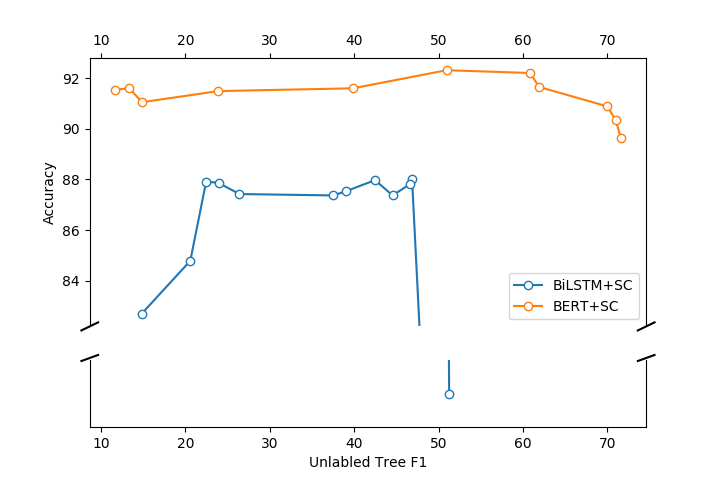
Figure 3: The relation between the accuracy and unlabeled tree F1 on SST2-S.

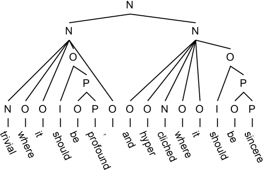
(a) Double irealistic blocking.

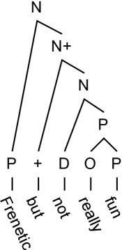
(b) Negation in conflict resolution.

Figure 4: Semantic trees of compound sentiment compositions, generated by BiLSTM+SCM. We flatten the polarity propagation rules for compactness.

4.4 Qualitative Study

We qualitatively show a few examples to show our method can handle compound sentiment compositions in Figure 4. The first case is a sentence with two negative constituents joining by a coordinating conjunction, each of which has an irrealis blocking within. The second case is a sentence with negation under conflict resolution. For both cases, the prediction is not simple since the model is susceptible to the surface and literal meaning in the sentence, which might interfere the correct decision. Taking the sentiment composition explicitly, we can see that our method successfully judge the semantic role of different constituents, and finally compose plausible tree explanations.

5 Related Works

Sentiment composition is one of the key to sentiment analysis, which considers the semantic of a constituent from both recognition and composition views Polanyi and Zaenen (2006); Moilanen and Pulman (2007). That is, it decomposes the classification of a sentence into a hierarchical tree structure explicitly showing how the polarity of the sentence come from the composition of its sub-constituents. Early works are mainly based on manual rules and semantic lexicon that is constructed either manually Wilson et al. (2005); Kennedy and Inkpen (2006) or automatically Dong et al. (2015); Toledo-Ronen et al. (2018). Nowadays, represented via different forms of tree, sentiment composition is often learned explicitly or implicitly in the end-to-end learning manner of neural network models.

Common tree forms include untagged tree and sentiment tree, while the learning paradigm is also varied in literature. To be concrete, untagged tree can either be directly obtained from the external syntactic parser Socher et al. (2012); Tai et al. (2015); Liu et al. (2017a, b); Kim et al. (2019), or serve as a latent variable learned implicitly Yogatama et al. (2017); Maillard and Clark (2018); Choi et al. (2018); Havrylov et al. (2019); Chowdhury and Caragea (2021). Compared to the untagged one, sentiment tree offers more information about sentiment polarity of each constituent in the tree. As the most representative resource in this form, SST Socher et al. (2013) formalizes sentiment composition as a parsing task, motivating lots of works to learn the tree supervisedly Teng and Zhang (2017); Zhang and Zhang (2019); Zhang et al. (2019). Sentiment tree is also a popular explanation form for post-hoc interprebility since it can provide hierahical attribution scores Chen et al. (2020); Zhang et al. (2020). While both existing forms are useful, they are suboptimal due to their in-ability to explicitly interpret sentiment composition, which our proposed semantic tree fills this gap.

6 Conclusions

In this paper, we present semantic tree to explicitly interpret sentiment compositions in sentiment classification. we carefully design a grammar under each compositions from the linguistic inspiration, and learn to extract semantic tree explanations without full annotations. Quantitative and qualitative results demonstrate that our method is effective and can generate plausible tree explanations.

7 Limitations & Ethics Statement

Our method is first limited by the proposed grammar that doesn’t cover all the realistic cases. As shown in Table 1, there are still a few cases in the randomly sampled 100 examples that none of the defined rules can explain. Secondly, the time complexity of our method is the cube of the sentence length, limiting its direct applications on long documents. So we have to classify the document based on classification of individual sentences, which might be problematic since the sentiment of different sentences in the document may affect each other.

All the experiments in this paper are conducted on public available datasets, which has no data privacy concerns. Meanwhile, this paper doesn’t involve human annotations, so there are no related ethical concerns.

Appendix A Binary Rules

Table 6 shows all the binary rules contained in the proposed SCG.

Appendix B Functional Lexicon

Table 7 lists functional lexicon in the manually constructed lexicon.

Composition	Rules
Polarity propagation	$O\ P\rightarrow P$ $P\ O\rightarrow P$ $O\ N\rightarrow N$ $N\ O\rightarrow N$	$O\ O\rightarrow O$ $P\ P\rightarrow P$ $N\ N\rightarrow N$
Negation	$D\ P\rightarrow N$ $D\ N\rightarrow P$	$P\ D\rightarrow N$ $N\ D\rightarrow P$
Conflict resolution	$P\ +\rightarrow P^{+}$ $N\ +\rightarrow N^{+}$ $+\ P\rightarrow P^{+}$ $+\ N\rightarrow N^{+}$ $P^{+}\ +\rightarrow P^{+}$ $N^{+}\ +\rightarrow N^{+}$ $+\ P^{+}\rightarrow P^{+}$ $+\ N^{+}\rightarrow N^{+}$ $P\ -\rightarrow P^{-}$ $N\ +\rightarrow N^{-}$ $-\ P\rightarrow P^{-}$ $-\ N\rightarrow N^{-}$ $P^{-}\ -\rightarrow P^{-}$ $N^{-}\ +\rightarrow N^{-}$ $-\ P^{-}\rightarrow P^{-}$ $-\ N^{-}\rightarrow N^{-}$ $P^{+}\ O\rightarrow P^{+}$ $N^{+}\ O\rightarrow N^{+}$ $P^{-}\ O\rightarrow P^{-}$ $N^{-}\ O\rightarrow N^{-}$ $O\ P^{+}\rightarrow P^{+}$ $O\ N^{+}\rightarrow N^{+}$ $O\ P^{-}\rightarrow P^{-}$ $O\ P-\rightarrow P^{-}$	$N\ P^{+}\rightarrow P$ $N^{-}\ P^{+}\rightarrow P$ $N^{-}\ P\rightarrow P$ $P^{+}\ N\rightarrow P$ $P^{+}\ N^{-}\rightarrow P$ $P\ N^{-}\rightarrow P$ $N\ P^{-}\rightarrow N$ $N^{+}\ P^{-}\rightarrow N$ $N^{+}\ P\rightarrow N$ $P^{-}\ N\rightarrow N$ $P^{-}\ N^{+}\rightarrow N$ $P\ N^{+}\rightarrow N$
Irrealis blocking	$I\ P\rightarrow O$ $I\ N\rightarrow O$	$P\ I\rightarrow O$ $N\ I\rightarrow O$

Table 6: Binary rules in the proposed SCG.

Label	Words
Priority riser $+$	but, however, yet, whereas, still
Priority reducer $-$	although, though, despite, regardless, nevertheless, nonetheless
Irrealis blocker $I$	could, should, would, ought, supposed, if
Negator $D$	no, not, n’t, neither, nor, never, none, lack, without, cannot, aint, arent, barely, cant, couldnt, didnt, doesnt, dont, hardly, havent, few, isnt, merely, never, nothing, nobody, shouldnt, wasnt, werent, wont, wouldnt

Table 7: Funtional lexicon.

References

- Baccianella et al. (2010) Stefano Baccianella, Andrea Esuli, and Fabrizio Sebastiani. 2010. SentiWordNet 3.0: An enhanced lexical resource for sentiment analysis and opinion mining. In Proceedings of the Seventh International Conference on Language Resources and Evaluation (LREC’10), Valletta, Malta. European Language Resources Association (ELRA).
- Baker (1979) James K Baker. 1979. Trainable grammars for speech recognition. The Journal of the Acoustical Society of America, 65(S1):S132–S132.
- Bastings et al. (2019) Jasmijn Bastings, Wilker Aziz, and Ivan Titov. 2019. Interpretable neural predictions with differentiable binary variables. In Proceedings of the 57th Annual Meeting of the Association for Computational Linguistics, pages 2963–2977, Florence, Italy. Association for Computational Linguistics.
- Blitzer et al. (2007) John Blitzer, Mark Dredze, and Fernando Pereira. 2007. Biographies, Bollywood, boom-boxes and blenders: Domain adaptation for sentiment classification. In Proceedings of the 45th Annual Meeting of the Association of Computational Linguistics, pages 440–447, Prague, Czech Republic. Association for Computational Linguistics.
- Chen et al. (2020) Hanjie Chen, Guangtao Zheng, and Yangfeng Ji. 2020. Generating hierarchical explanations on text classification via feature interaction detection. In Proceedings of the 58th Annual Meeting of the Association for Computational Linguistics, pages 5578–5593, Online. Association for Computational Linguistics.
- Choi et al. (2018) Jihun Choi, Kang Min Yoo, and Sang-goo Lee. 2018. Learning to compose task-specific tree structures. In Proceedings of the Thirty-Second AAAI Conference on Artificial Intelligence, (AAAI-18), the 30th innovative Applications of Artificial Intelligence (IAAI-18), and the 8th AAAI Symposium on Educational Advances in Artificial Intelligence (EAAI-18), New Orleans, Louisiana, USA, February 2-7, 2018, pages 5094–5101. AAAI Press.
- Chomsky (1956) Noam Chomsky. 1956. Three models for the description of language. IRE Transactions on information theory, 2(3):113–124.
- Chomsky (1963) Noam Chomsky. 1963. Formal properties of grammars. Handbook of Math. Psychology, 2:328–418.
- Chowdhury and Caragea (2021) Jishnu Ray Chowdhury and Cornelia Caragea. 2021. Modeling hierarchical structures with continuous recursive neural networks. In International Conference on Machine Learning, pages 1975–1988. PMLR.
- Dang et al. (2020) Nhan Cach Dang, María N Moreno-García, and Fernando De la Prieta. 2020. Sentiment analysis based on deep learning: A comparative study. Electronics, 9(3):483.
- Daniel (1967) H Younger Daniel. 1967. Recognition and parsing of context-free languages in time n3. Information and control, 10(2):189–208.
- De Cao et al. (2020) Nicola De Cao, Michael Sejr Schlichtkrull, Wilker Aziz, and Ivan Titov. 2020. How do decisions emerge across layers in neural models? interpretation with differentiable masking. In Proceedings of the 2020 Conference on Empirical Methods in Natural Language Processing (EMNLP), pages 3243–3255, Online. Association for Computational Linguistics.
- Devlin et al. (2019) Jacob Devlin, Ming-Wei Chang, Kenton Lee, and Kristina Toutanova. 2019. BERT: Pre-training of deep bidirectional transformers for language understanding. In Proceedings of the 2019 Conference of the North American Chapter of the Association for Computational Linguistics: Human Language Technologies, Volume 1 (Long and Short Papers), pages 4171–4186, Minneapolis, Minnesota. Association for Computational Linguistics.
- Dong et al. (2015) Li Dong, Furu Wei, Shujie Liu, Ming Zhou, and Ke Xu. 2015. A statistical parsing framework for sentiment classification. Computational Linguistics, 41(2):265–308.
- Durrett and Klein (2015) Greg Durrett and Dan Klein. 2015. Neural CRF parsing. In Proceedings of the 53rd Annual Meeting of the Association for Computational Linguistics and the 7th International Joint Conference on Natural Language Processing (Volume 1: Long Papers), pages 302–312, Beijing, China. Association for Computational Linguistics.
- Eisner (2016) Jason Eisner. 2016. Inside-outside and forward-backward algorithms are just backprop (tutorial paper). In Proceedings of the Workshop on Structured Prediction for NLP, pages 1–17, Austin, TX. Association for Computational Linguistics.
- Finkel et al. (2008) Jenny Rose Finkel, Alex Kleeman, and Christopher D. Manning. 2008. Efficient, feature-based, conditional random field parsing. In Proceedings of ACL-08: HLT, pages 959–967, Columbus, Ohio. Association for Computational Linguistics.
- Havrylov et al. (2019) Serhii Havrylov, Germán Kruszewski, and Armand Joulin. 2019. Cooperative learning of disjoint syntax and semantics. In Proceedings of the 2019 Conference of the North American Chapter of the Association for Computational Linguistics: Human Language Technologies, Volume 1 (Long and Short Papers), pages 1118–1128, Minneapolis, Minnesota. Association for Computational Linguistics.
- Hochreiter and Schmidhuber (1997) Sepp Hochreiter and Jürgen Schmidhuber. 1997. Long short-term memory. Neural computation, 9(8):1735–1780.
- Kasami (1965) Tadao Kasami. 1965. An efficient recognition and syntax algorithm for context-free languages. Technical report, Air Force Cambridge Research Lab.
- Kennedy and Inkpen (2006) Alistair Kennedy and Diana Inkpen. 2006. Sentiment classification of movie reviews using contextual valence shifters. Computational intelligence, 22(2):110–125.
- Kim et al. (2020) Siwon Kim, Jihun Yi, Eunji Kim, and Sungroh Yoon. 2020. Interpretation of NLP models through input marginalization. In Proceedings of the 2020 Conference on Empirical Methods in Natural Language Processing (EMNLP), pages 3154–3167, Online. Association for Computational Linguistics.
- Kim et al. (2019) Taeuk Kim, Jihun Choi, Daniel Edmiston, Sanghwan Bae, and Sang-goo Lee. 2019. Dynamic compositionality in recursive neural networks with structure-aware tag representations. In The Thirty-Third AAAI Conference on Artificial Intelligence, AAAI 2019, The Thirty-First Innovative Applications of Artificial Intelligence Conference, IAAI 2019, The Ninth AAAI Symposium on Educational Advances in Artificial Intelligence, EAAI 2019, Honolulu, Hawaii, USA, January 27 - February 1, 2019, pages 6594–6601. AAAI Press.
- Kitaev et al. (2019) Nikita Kitaev, Steven Cao, and Dan Klein. 2019. Multilingual constituency parsing with self-attention and pre-training. In Proceedings of the 57th Annual Meeting of the Association for Computational Linguistics, pages 3499–3505, Florence, Italy. Association for Computational Linguistics.
- Kitaev and Klein (2018) Nikita Kitaev and Dan Klein. 2018. Constituency parsing with a self-attentive encoder. In Proceedings of the 56th Annual Meeting of the Association for Computational Linguistics (Volume 1: Long Papers), pages 2676–2686, Melbourne, Australia. Association for Computational Linguistics.
- Lei et al. (2016) Tao Lei, Regina Barzilay, and Tommi Jaakkola. 2016. Rationalizing neural predictions. In Proceedings of the 2016 Conference on Empirical Methods in Natural Language Processing, pages 107–117, Austin, Texas. Association for Computational Linguistics.
- Li et al. (2016) Jiwei Li, Will Monroe, and Dan Jurafsky. 2016. Understanding neural networks through representation erasure. ArXiv preprint, abs/1612.08220.
- Liu et al. (2017a) Pengfei Liu, Xipeng Qiu, and Xuanjing Huang. 2017a. Adaptive semantic compositionality for sentence modelling. In Proceedings of the Twenty-Sixth International Joint Conference on Artificial Intelligence, IJCAI 2017, Melbourne, Australia, August 19-25, 2017, pages 4061–4067. ijcai.org.
- Liu et al. (2017b) Pengfei Liu, Xipeng Qiu, and Xuanjing Huang. 2017b. Dynamic compositional neural networks over tree structure. In Proceedings of the Twenty-Sixth International Joint Conference on Artificial Intelligence, IJCAI 2017, Melbourne, Australia, August 19-25, 2017, pages 4054–4060. ijcai.org.
- Loshchilov and Hutter (2017) Ilya Loshchilov and Frank Hutter. 2017. SGDR: stochastic gradient descent with warm restarts. In 5th International Conference on Learning Representations, ICLR 2017, Toulon, France, April 24-26, 2017, Conference Track Proceedings. OpenReview.net.
- Loughran and McDonald (2011) Tim Loughran and Bill McDonald. 2011. When is a liability not a liability? textual analysis, dictionaries, and 10-ks. The Journal of finance, 66(1):35–65.
- Maillard and Clark (2018) Jean Maillard and Stephen Clark. 2018. Latent tree learning with differentiable parsers: Shift-reduce parsing and chart parsing. In Proceedings of the Workshop on the Relevance of Linguistic Structure in Neural Architectures for NLP, pages 13–18, Melbourne, Australia. Association for Computational Linguistics.
- Moilanen and Pulman (2007) Karo Moilanen and Stephen Pulman. 2007. Sentiment composition.
- Pang and Lee (2005) Bo Pang and Lillian Lee. 2005. Seeing stars: Exploiting class relationships for sentiment categorization with respect to rating scales. In Proceedings of the 43rd Annual Meeting of the Association for Computational Linguistics (ACL’05), pages 115–124, Ann Arbor, Michigan. Association for Computational Linguistics.
- Polanyi and Zaenen (2006) Livia Polanyi and Annie Zaenen. 2006. Contextual valence shifters. In Computing attitude and affect in text: Theory and applications, pages 1–10. Springer.
- Qian (1999) Ning Qian. 1999. On the momentum term in gradient descent learning algorithms. Neural networks, 12(1):145–151.
- Raffel et al. (2020) Colin Raffel, Noam Shazeer, Adam Roberts, Katherine Lee, Sharan Narang, Michael Matena, Yanqi Zhou, Wei Li, Peter J Liu, et al. 2020. Exploring the limits of transfer learning with a unified text-to-text transformer. J. Mach. Learn. Res., 21(140):1–67.
- Ribeiro et al. (2016) Marco Túlio Ribeiro, Sameer Singh, and Carlos Guestrin. 2016. "why should I trust you?": Explaining the predictions of any classifier. In Proceedings of the 22nd ACM SIGKDD International Conference on Knowledge Discovery and Data Mining, San Francisco, CA, USA, August 13-17, 2016, pages 1135–1144. ACM.
- Socher et al. (2012) Richard Socher, Brody Huval, Christopher D. Manning, and Andrew Y. Ng. 2012. Semantic compositionality through recursive matrix-vector spaces. In Proceedings of the 2012 Joint Conference on Empirical Methods in Natural Language Processing and Computational Natural Language Learning, pages 1201–1211, Jeju Island, Korea. Association for Computational Linguistics.
- Socher et al. (2011) Richard Socher, Cliff Chiung-Yu Lin, Andrew Y. Ng, and Christopher D. Manning. 2011. Parsing natural scenes and natural language with recursive neural networks. In Proceedings of the 28th International Conference on Machine Learning, ICML 2011, Bellevue, Washington, USA, June 28 - July 2, 2011, pages 129–136. Omnipress.
- Socher et al. (2013) Richard Socher, Alex Perelygin, Jean Wu, Jason Chuang, Christopher D. Manning, Andrew Ng, and Christopher Potts. 2013. Recursive deep models for semantic compositionality over a sentiment treebank. In Proceedings of the 2013 Conference on Empirical Methods in Natural Language Processing, pages 1631–1642, Seattle, Washington, USA. Association for Computational Linguistics.
- Strout et al. (2019) Julia Strout, Ye Zhang, and Raymond Mooney. 2019. Do human rationales improve machine explanations? In Proceedings of the 2019 ACL Workshop BlackboxNLP: Analyzing and Interpreting Neural Networks for NLP, pages 56–62, Florence, Italy. Association for Computational Linguistics.
- Taboada et al. (2011) Maite Taboada, Julian Brooke, Milan Tofiloski, Kimberly Voll, and Manfred Stede. 2011. Lexicon-based methods for sentiment analysis. Computational Linguistics, 37(2):267–307.
- Tai et al. (2015) Kai Sheng Tai, Richard Socher, and Christopher D. Manning. 2015. Improved semantic representations from tree-structured long short-term memory networks. In Proceedings of the 53rd Annual Meeting of the Association for Computational Linguistics and the 7th International Joint Conference on Natural Language Processing (Volume 1: Long Papers), pages 1556–1566, Beijing, China. Association for Computational Linguistics.
- Taylor et al. (2003) Ann Taylor, Mitchell Marcus, and Beatrice Santorini. 2003. The penn treebank: an overview. Treebanks, pages 5–22.
- Teng and Zhang (2017) Zhiyang Teng and Yue Zhang. 2017. Head-lexicalized bidirectional tree LSTMs. Transactions of the Association for Computational Linguistics, 5:163–177.
- Toledo-Ronen et al. (2018) Orith Toledo-Ronen, Roy Bar-Haim, Alon Halfon, Charles Jochim, Amir Menczel, Ranit Aharonov, and Noam Slonim. 2018. Learning sentiment composition from sentiment lexicons. In Proceedings of the 27th International Conference on Computational Linguistics, pages 2230–2241, Santa Fe, New Mexico, USA. Association for Computational Linguistics.
- Williams et al. (2018) Adina Williams, Andrew Drozdov, and Samuel R. Bowman. 2018. Do latent tree learning models identify meaningful structure in sentences? Transactions of the Association for Computational Linguistics, 6:253–267.
- Wilson et al. (2005) Theresa Wilson, Janyce Wiebe, and Paul Hoffmann. 2005. Recognizing contextual polarity in phrase-level sentiment analysis. In Proceedings of Human Language Technology Conference and Conference on Empirical Methods in Natural Language Processing, pages 347–354, Vancouver, British Columbia, Canada. Association for Computational Linguistics.
- Yadav and Vishwakarma (2020) Ashima Yadav and Dinesh Kumar Vishwakarma. 2020. Sentiment analysis using deep learning architectures: a review. Artificial Intelligence Review, 53(6):4335–4385.
- Yogatama et al. (2017) Dani Yogatama, Phil Blunsom, Chris Dyer, Edward Grefenstette, and Wang Ling. 2017. Learning to compose words into sentences with reinforcement learning. In 5th International Conference on Learning Representations, ICLR 2017, Toulon, France, April 24-26, 2017, Conference Track Proceedings. OpenReview.net.
- Zhang et al. (2020) Die Zhang, Huilin Zhou, Xiaoyi Bao, Da Huo, Ruizhao Chen, Xu Cheng, Hao Zhang, Mengyue Wu, and Quanshi Zhang. 2020. Interpreting hierarchical linguistic interactions in dnns.
- Zhang et al. (2019) Liwen Zhang, Kewei Tu, and Yue Zhang. 2019. Latent variable sentiment grammar. In Proceedings of the 57th Annual Meeting of the Association for Computational Linguistics, pages 4642–4651, Florence, Italy. Association for Computational Linguistics.
- Zhang and Zhang (2019) Yuan Zhang and Yue Zhang. 2019. Tree communication models for sentiment analysis. In Proceedings of the 57th Annual Meeting of the Association for Computational Linguistics, pages 3518–3527, Florence, Italy. Association for Computational Linguistics.
- Zhong et al. (2019) Ruiqi Zhong, Steven Shao, and Kathleen McKeown. 2019. Fine-grained sentiment analysis with faithful attention. ArXiv preprint, abs/1908.06870.
- Zhu et al. (2015) Xiao-Dan Zhu, Parinaz Sobhani, and Hongyu Guo. 2015. Long short-term memory over recursive structures. In Proceedings of the 32nd International Conference on Machine Learning, ICML 2015, Lille, France, 6-11 July 2015, volume 37 of JMLR Workshop and Conference Proceedings, pages 1604–1612. JMLR.org.