Un-screened forces in Quark-Gluon Plasma ?

Abstract

We study the correlator of temporal Wilson lines at non-zero temperature in 2+1 flavor lattice QCD with the aim to define the heavy quark-antiquark potential at non-zero temperature. For temperatures $153\leavevmode\nobreak\ {\rm MeV}\leq T\leq 352\leavevmode\nobreak\ {\rm MeV}$ the spectral representation of this correlator is consistent with a broadened peak in the spectral function, position or width of which then defines the real or imaginary parts of the heavy quark-antiquark potential at non-zero temperature, respectively. We find that the real part of the potential is not screened contrary to the widely-held expectations. We comment on how this fact may modify the picture of quarkonium melting in the quark-gluon plasma.

Introduction At very high temperatures the strongly interacting matter undergoes a transition to a new state called quark-gluon plasma (QGP). Creating and studying the properties of QGP is the goal of large experimental programs in heavy-ion collisions at RHIC and LHC [1].

The question of in-medium modifications of the forces between heavy quark $Q$ and antiquark $\bar{Q}$ generated a lot of interest since the seminal paper by Matsui and Satz [2]. They conjectured that color screening in QGP will make the $Q\bar{Q}$ interaction short ranged, and therefore quarkonium states cannot be formed in QGP. Thus, QGP formation in heavy-ion collision will lead to quarkonium suppression. The study of quarkonium production in heavy-ion collisions is a large part of the experimental heavy-ion program, see e.g. Ref. [3] for a recent review.

The idea of having a screened potential between heavy quarks in QGP is closely related to the exponential screening of the free energy of infinitely heavy quarks in QGP, which is well established by lattice QCD calculations, see e.g. Ref. [4] for a review. However, the free energy of heavy quarks describes the in-medium interaction of heavy quarks at macroscopic time scales much larger than the inverse temperature. For understanding the quarkonium properties in QGP one needs to know if and how the heavy $Q\bar{Q}$ potential is modified at scales comparable to the internal time scale of quarkonium. The effective field theory (EFT) approach provides a natural framework to address this problem at high temperatures when the weak-coupling approach is applicable [5, 6]. Depending on the separation of the bound-state scales and the thermal scales the heavy $Q\bar{Q}$ potential can be modified by QGP and also acquire an imaginary part. In general, however, the real part of this potential does not have a screened form in this approach [6]. How to study the modification of heavy $Q\bar{Q}$ interactions in QGP beyond weak coupling remains an unsolved problem. However, we could define the heavy $Q\bar{Q}$ potential at non-zero temperature ($T>0$) in analogy with the zero temperature ($T=0$) case in terms of the Wilson loops of size $\tau\times r$ [7]. We can write the following spectral representation of the Wilson loops in terms of the $r$-dependent spectral function

$$W(\tau,r,T)=\int_{-\infty}^{+\infty}d\omega e^{-\omega\tau}\rho_{r}(\omega,T).$$ (1)

The distance $r$ between the infinitely heavy quark and antiquark acts as the label of the spectral function. At $T=0$, the spectral function’s lowest delta function peak corresponds to the ground state potential. We expect that there will be a dominant peak in the spectral function with non-zero width for not too high temperatures. The position of this peak determines the real part of the potential, while its width determines the potential’s imaginary part [7]. For very high temperatures the spectral function may lack a well-defined peak such that a potential cannot be defined. While the relation between the above defined complex potential and the EFT concept of the complex potential is an unsolved problem, too, the existence of a well-defined peak in $\rho_{r}(\omega,T)$ is necessary, yet not a sufficient condition for a potential picture of heavy quarkonium at $T>0$.

In this paper we present calculations of the real part of the potential at $T>0$ in 2+1 flavor QCD using the lattice QCD approach. We also estimate the imaginary part of the potential. There have been several attempts to calculate the complex potential at $T>0$ both in quenched QCD [7, 8] as well as in 2+1 flavor QCD [9, 10]. The state of the art calculation of the complex potential in 2+1 flavor QCD has been performed using lattices with temporal extent $N_{\tau}=12$, and thus at a single lattice spacing per temperature. The new results are based on several lattice spacings and several values of $N_{\tau}$ in the range $N_{\tau}=16-36$.

Details of the lattice QCD calculations In lattice QCD calculations one often considers correlators of Wilson lines in Coulomb gauge instead of Wilson loops since these contain the same physical information and are less noisy, see the discussions in Ref. [10] and in the supplemental material. We performed lattice QCD calculations of Wilson line correlators in 2+1 flavor QCD using highly improved staggered quark (HISQ) action [11] and tree level improved gauge action [12, 13] for physical strange quark mass, $m_{s}$ and two sets of light ($u$ and $d$) quark mass, $m_{l}=m_{s}/5$ and $m_{l}=m_{s}/20$. The latter corresponds to almost physical pion mass, $m_{\pi}=161$ MeV in the continuum limit. For the smallest lattice spacing, we cover only $T\geq 195$ MeV, and thus used $m_{l}=m_{s}/5$, since the light-quark mass effects are suppressed at these temperatures. We performed lattice calculations with $N_{\tau}=16-36$ in the temperature range $153\leavevmode\nobreak\ {\rm MeV}\leq T\leq 352$ MeV. For these large temporal extents, noise reduction methods have to be used in the calculations. We use gradient flow [14] for noise reduction. To obtain further noise reduction in the Wilson line correlators at large spatial distances we require that these correlators are smooth functions of distance $r$ for each value $\tau$. By performing a smooth interpolation of the Wilson line correlators in $r$ for a given $\tau$ and then replacing the original data points with the interpolated values we obtain a less noisy correlator. To aid the reconstruction of the spectral function we also performed calculations on $N_{\tau}=64$ and $N_{\tau}=56$ lattices, which we refer to as $T=0$ lattices. Further details of the lattice QCD calculations, in particular, the lattice parameters and the used noise reduction techniques are presented in the supplemental materials.

Figure 1: The effective masses at $T=0$ and at $T\simeq 220$ MeV for $r\simeq 0.7$ fm and three different lattice spacings, $a=0.0280$ fm (circles), $a=0.0404$ fm (squares) and $a=0.0493$ fm (triangles). The green symbols correspond to the subtracted effective masses. The lines show the fits discussed in the text.

Analysis and Results. To analyze the lattice results on the Wilson line correlator $W(\tau,r,T)$ in Eq. (1) it is useful to consider the effective mass defined as

$$m_{\text{eff}} =-\partial_{\tau}\ln W(\tau,r,T)$$

$$=\frac{1}{a}\ln\Bigg{[}\frac{W(\tau+a,r,T)}{W(\tau,r,T)}\Bigg{]}\leavevmode\nobreak\ ,$$ (2)

where the last equation applies to the case of non-zero lattice spacing. At $T=0$, the effective mass will decrease with increasing $\tau$, and for sufficiently large $\tau$ it will reach a plateau, since the spectral function is positive definite and has the lowest ground state delta function peak followed by many excited states for $\omega$ above the ground state. We show the results for the effective masses in Fig. 1. We see that at $T=0$ the effective mass decreases with increasing $\tau$ with the exception of the data at smallest $\tau$ and approaches the plateau for $\tau$ around $0.5$ fm. The non-monotonic behavior of the effective mass is due to the smearing artifacts coming from the gradient flow, see supplemental material. Except for very small $\tau$, $m_{\text{eff}}$ decreases at $T>0$ with increasing $\tau$ for all $\tau$ values and does not reach a plateau. This is not related to the small time extent $1/T$, since the effective mass at $T=0$ reaches a plateau for $\tau=0.5$ fm, which is considerably smaller than $1/T$. This rather means that there is no stable ground state at non-zero temperature. We see from Fig. 1 that the effective masses show neither lattice spacing nor sea quark mass dependence for $T>200$ MeV. This implies that for these temperatures using $m_{l}=m_{s}/5$ is equivalent to using the physical light quark mass and that our results are essentially in the continuum limit. We also compared the effective masses corresponding to different lattice spacings at lower temperatures and found no dependence on the lattice spacing.

At small $\tau$ the difference between the $T=0$ or $T>0$ effective masses is the smallest, and the $\tau$-dependence of the effective masses at $T=0$ or $T>0$ is rather similar, see Fig. 1. This implies that the relevant high $\omega$ part of the spectral function is not affected much by the medium. Therefore, for the spectral function we write the Ansatz $\rho_{r}(\omega,T)=\rho_{r}^{\text{med}}(\omega,T)+\rho_{r}^{\text{high}}(\omega)$, where $\rho_{r}^{\text{med}}(\omega,T)$ contains all the temperature dependence of the spectral function, and $\rho_{r}^{\text{high}}(\omega)$ is the temperature-independent high $\omega$ part of the spectral function that has its support much above the ground state peak. We can also define the high $\omega$ part of the Wilson line correlator as

$$W^{\text{high}}(\tau,r)=\int_{-\infty}^{\infty}d\omega\rho^{\text{high}}_{r}(\omega)e^{-\omega\tau},$$ (3)

which can be easily obtained from our correlators at $T=0$. We can simplify the analysis of the correlators at $T>0$ by subtracting $W^{\text{high}}(\tau,r)$. The subtracted correlator will only be sensitive to the medium dependent part of the spectral function $\rho_{r}^{\text{med}}$. The effective masses from the subtracted correlators at $T>0$ are also shown in Fig. 1. We note that the non-monotonic behavior in $\tau$ due to smearing artifacts is absent in the effective masses corresponding to the subtracted correlator, and therefore, these artifacts will not affect the extraction of $\rho^{\text{med}}_{r}$. The subtracted effective mass shows linear behavior in $\tau$ for small $\tau$, indicating that the dominant ground state peak has broadened. If the ground state peak would be described by a Gaussian form $m_{\text{eff}}$ would decrease linearly in $\tau$ [10]. As discussed in Ref. [10] at $T>0$ in addition to the ground state peak there is also a contribution to the spectral function at small $\omega$ representing a heavy $Q\bar{Q}$ state propagating forward in Euclidean time interacting with a backward propagating light state from the medium. Based on these considerations we make the following Ansatz for the medium dependent part of the spectral function $\rho_{r}^{\text{med}}(\omega,T)=\rho^{\text{peak}}_{r}(\omega,T)+\rho_{r}^{\text{low}}(\omega,T)$, where $\rho_{r}^{\text{peak}}$ is the broadened ground state peak and $\rho_{r}^{\text{low}}$ is the contribution to the spectral function for $\omega$ much below the dominant peak. We expect that $\rho_{r}^{\text{low}}$ is much smaller than $\rho_{r}^{\text{peak}}$ but it dominates the correlator at $\tau$ around $1/T$. This part of the spectral function explains the rapid drop of $m_{\text{eff}}$ at large $\tau$ [10] that can be seen in Fig. 1.

A physically appealing parametrization of $\rho^{\text{peak}}$ is a Lorentzian form. However, a Lorentzian form is only valid in the vicinity of the peak. In general, we can assume that the correlator has a pole at some complex $\omega$, so

$$\rho_{r}^{\text{peak}}(\omega,T) =\frac{1}{\pi}{\rm Im}\frac{A_{r}(T)}{\omega-{\rm Re}V(r,T)-i\Gamma(\omega,r,T)}$$

$$=\frac{1}{\pi}\frac{A_{r}(T)\Gamma(\omega,r,T)}{[\omega-{\rm Re}V(r,T)]^{2}+\Gamma^{2}(\omega,r,T)}.$$ (4)

For $\omega\simeq{\rm Re}V(r,T)$ we can approximate $\Gamma(\omega,r,T)$ by a constant: $\Gamma(\omega,r,T)\simeq\Gamma_{L}(r,T)$. However, for $\omega$ values far away from the peak $\Gamma(\omega,r,T)$ will quickly go to zero. The self-consistent $T$-matrix calculation of heavy $Q\bar{Q}$ propagators indeed shows an exponential decrease of $\Gamma(\omega,r,T)$ away from the peak [15]. To incorporate this feature of the spectral function in our analysis we assume that $\rho_{r}^{\text{peak}}$ is given by $\Gamma_{L}(r,T)/([\omega-{\rm Re}V(r,T)]^{2}+\Gamma_{L}^{2}(r,T))$ for $|\omega-{\rm Re}V(r,T)|\lesssim\Gamma_{L}(r,T)$ and is zero otherwise. Such a cut Lorentzian form gives rise to an almost linear behavior of $m_{\text{eff}}$ at small $\tau$, too, as required by the lattice data.

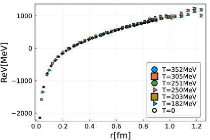
Figure 2: The real part of the potential as a function of $r$ at different temperatures. We show results for three different lattice spacings, $a=0.0280$ fm (circles), $a=0.0404$ fm (squares) and $a=0.0493$ fm (triangles).

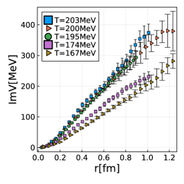
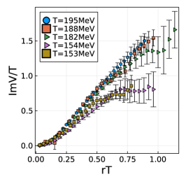
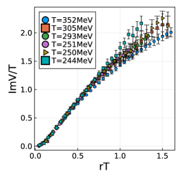
Figure 3: The estimate of the imaginary part of the potential from the fit using cut Lorentzian form as a function of $rT$ for different temperatures. The three panels focus on different temperature ranges. The circles correspond to the smallest lattice spacing $a=0.0280$ fm, the squares to the next-to-smallest lattice spacing, $a=0.0404$ fm, and the triangles correspond to the largest lattice spacing $a=0.0493$ fm.

The most general parametrization of $\rho_{r}^{\text{low}}$ would be a sum of delta functions at $\omega$ well below the dominant peak position. However, to describe our effective mass data even a single delta function at sufficiently small $\omega$, $\rho_{r}^{\text{low}}(\omega,T)=c_{r}^{\text{low}}(T)\delta(\omega-\omega_{r}^{\text{low}}(T))$ turns out as sufficient.

With these forms of $\rho_{r}^{\text{peak}}$ and $\rho_{r}^{\text{low}}$ we fitted the lattice data on the effective mass and determined the fit parameters ${\rm Re}V(r,T)$, $\Gamma_{L}(r,T)$, $c_{r}^{\text{low}}(T)/A_{r}(T)$ and $\omega_{r}^{\text{low}}(T)$. A sample fit is shown in Fig. 1 and details of the fits are discussed in the Supplemental Material. We typically find that $c_{r}^{\text{low}}(T)/A_{r}(T)<5\cdot 10^{-4}$ and decreases with decreasing $r$, while $\omega_{r}^{\text{low}}(T)$ is between (1.8-3.8) GeV below the peak position $\omega={\rm Re}V(r,T)$. The results for ${\rm Re}V(r,T)$ are shown in Fig. 2. As one can see from the figure the real part of the potential at $T>0$ is temperature independent and agrees with the $T=0$ potential very well. This is not completely unexpected, as the value of the effective mass at small $\tau$ is close to the vacuum result, c.f. Fig. 1. We find that the peak position is insensitive to the detailed shape of $\rho_{r}^{\text{peak}}$, i.e. for $\rho_{r}^{\text{peak}}$ with a Gaussian form we find the same peak position within errors. Thus our lattice QCD results show that the real part of the potential is unscreened.

As discussed above the imaginary part of the potential is defined as the width of the ground state peak at $T>0$. If we knew the exact form of the spectral function we would fit it in the vicinity of the peak with a Lorentzian form, whose width parameter would give the potential’s imaginary part. This has been explicitly checked for the spectral function of an infinitely heavy $Q\bar{Q}$ pair calculated in hard thermal loop perturbation theory [16]. The correlator on the other hand is sensitive to all the details of the spectral function, in particular to $\rho_{r}^{\text{low}}$ and the tails of $\rho_{r}^{\text{peak}}$, and not just the behavior of $\rho_{r}^{\text{peak}}$ in the vicinity of the peak. For this reason, the parameter $\Gamma_{L}$ cannot be considered as ${\rm Im}V$. A better way to characterize the imaginary part is to consider the cumulants of $\rho_{r}^{\text{peak}}$. The first two cumulants are defined as $c_{1}=\langle\omega\rangle$ and $c_{2}=\langle\omega\rangle^{2}-\langle\omega^{2}\rangle$, where $\langle\dots\rangle=\int d\omega\dots$. In the case of the Gaussian, the second cumulant of the spectral function is the width parameter. In the case of the cut Lorentzian, it is proportional to the parameter $\Gamma_{L}$. Furthermore, if $c_{r}^{\text{low}}/A_{r}$ is very small, $\rho_{r}^{\text{peak}}$ determines the behavior of the Wilson line correlator around $\tau=0$. Therefore, the second cumulant of $\rho_{r}^{\text{peak}}$ determines the slope of the effective mass at small $\tau$, which is well defined from the lattice data, see the Supplemental material. Thus the second cumulant of $\rho_{r}^{\text{peak}}$ is a good proxy for the $r$ and temperature dependence of ${\rm Im}V$. In Fig. 3 we show the proxy for ${\rm Im}V$ as a function of distance $r$ for different temperatures. We scaled the $x$- and $y$-axes by the temperature in this figure. We see that for $180\leavevmode\nobreak\ {\rm MeV}<T\leq 352$ MeV the numerical results for ${\rm Im}V$ scale with the temperature, i.e. the imaginary part of the potential depends only on $rT$ and is proportional to the temperature. This is in qualitative agreement with the weak-coupling results. In the above temperature range, the dependence on the light-quark mass is very small. Thus we see again here that it is justified to perform lattice QCD calculations only for $m_{l}=m_{s}/5$. We also see no apparent dependence on the lattice spacing. This means that our results are very close to the continuum limit. For $T<180$ MeV the simple scaling with the temperature does not work. This is not surprising, since the dynamics of the heavy $Q\bar{Q}$ pair are expected to be quite complicated near the chiral transition. Since for $rT\simeq 1$ the imaginary part of the potential is larger than the temperature, the forces between heavy quarks are damped very quickly, i.e. on the time scale comparable to or shorter than the thermal scale. During that short time scale, the chromo-electric field between the heavy $Q$ and $\bar{Q}$ cannot adjust itself to the medium. The chromo-electric force between the heavy quarks is simply damped away, and the heavy $Q$ and $\bar{Q}$ will not interact. This picture of quarkonium melting is very different from the one proposed by Matsui and Satz.

Conclusion. We studied the complex heavy quark-antiquark potential at non-zero temperature in 2+1 flavor QCD using lattice calculations with a large temporal extent. We have found that contrary to some common expectations the real part of the potential is not screened for temperatures $153\leavevmode\nobreak\ {\rm MeV}\leq T\leq 352$ MeV. We also found that the dissipative effects on the chromo-electric forces between the heavy quarks, encoded in the imaginary part of the potential are very large and likely will lead to quarkonium dissolution.

Supplementary Material

In these supplemental materials, we present the technical details of our calculations of the complex quark anti-quark potential at non-zero temperature.

I Lattice QCD setup

As mentioned in the paper, we generate gauge configurations on $N_{x}^{3}\times N_{\tau}$ lattices using the HISQ action for quarks and the Symanzik-improved Lüscher-Weisz action for gluons. The calculations have been performed at the physical strange quark mass and light quark masses $m_{l}=m_{s}/5$ in a fixed scale approach on $96^{3}\times N_{\tau}$ lattices for the bare gauge coupling $\beta=10/g_{0}^{2}=8.249$, corresponding to a lattice spacing of $a=0.0280$ fm. We also performed calculations on coarser lattices with $\beta=7.825$ ($a=0.0404$ fm) and $\beta=7.596$ ($a=0.0493$ fm) at almost physical light quark masses $m_{l}=m_{s}/20$, corresponding to the pion mass of $161$ MeV in the continuum limit. The lattice spacing and thus the temperature scale $T=\nicefrac{{1}}{{(aN_{\tau})}}$ has been fixed using the $r_{1}$-scale determined in Ref. [18] with the value $r_{1}=0.3106\,\mathrm{fm}$ obtained in Ref. [19]. The value of the strange quark mass was obtained from the parametrization of the line of constant physics from Ref. [20]. The parameters of the lattice calculations including the lattice volume and the quark masses are given in Tables 1, 2, and 3.

The gauge configurations used in this study have been generated using a rational hybrid Monte-Carlo algorithm [21] with grants from PRACE on Juwels Booster and Marconi 100 and NERSC on Perlmutter using the SIMULATeQCD code [17]. We also used the MILC code on Cori at NERSC to generate the gauge configurations. Some of the gauge configurations have been generated on the USQCD cluster in JLab. After removing the initial trajectories for thermalization we arrived at the data set in Tables 1, 2, and 3. Every 5th trajectory has been used for $N_{x}=96$ and every 10th trajectory for $N_{x}=64$.

On the generated gauge configurations we calculated Wilson line correlators in Coulomb gauge with the aim of determining the static quark-antiquark ($Q\bar{Q}$) potential. We use Wilson line correlators instead of Wilson loops because these are much less noisy and provide more convenient access to distances at non-integer multiples of the lattice spacing. At $T=0$ both Wilson loops and Wilson line correlators in Coulomb gauge have been used for the determination of the $Q\bar{Q}$ potential, see e.g. Refs. [22, 23, 24, 18, 25]. In the case of Wilson loops, smearing should be applied to the spatial gauge links entering the Wilson loops in order to obtain a reasonable signal. In Ref. [10] both Wilson lines and Wilson loops with three-dimensional hyper-cubic (HYP) smearing [26] in the spatial gauge links have been studied at non-zero temperature. It was found there that the behavior of the Wilson line correlators and Wilson loops is fairly similar except for small $\tau$, where sensitivity to excited states is different, similar to the $T=0$ case [27]. At $T>0$ there are also some differences between the behavior of Wilson loops and Wilson line correlators at $\tau\simeq 1/T$, which are, however, not related to $Q\bar{Q}$ potential as discussed below. Thus both Wilson lines in Coulomb gauge and Wilson loops encode the same temperature modification of the $Q\bar{Q}$ potential. In Ref. [10] the calculations of the Wilson lines have been performed on $N_{\tau}=12$ lattices. Since we in this study use much larger $N_{\tau}$, also the temporal links have to be smeared. We use gradient flow [14] for the smearing of the temporal gauge links. More precisely we use Zeuthen flow [28]. For flow time $\tau_{F}$ the gauge links are smeared in a radius $\sqrt{8\tau_{F}}$. This radius should be much smaller than the inverse temperature. We use different flow times corresponding to the flow radius in the range $a-2.53a$ and study the sensitivity of our results to the flow time. For the final results presented in the paper, we use the smallest flow time that gives an acceptable signal. Since the signal deteriorates with increasing $N_{\tau}$ we use larger flow time for large $N_{\tau}$. The range of flow times and the specific values of flow times for which we show the final result are presented in Tables 1, 2, and 3 for $\beta=8.249,\leavevmode\nobreak\ 7.825$ and $7.596$, respectively.

After performing the gradient flow we fix the Coulomb gauge. The precision of Coulomb gauge fixing was set to $10^{-6}$. We also note that neither is the gradient flow the only option to smear the temporal gauge links nor is it a problem to fix the Coulomb gauge before performing the gradient flow, when studying Wilson line correlators. Previously we used HYP smearing after gauge fixing for the temporal gauge links when calculating the Wilson line correlators at $T>0$ [29] and found that the temperature and the $\tau$ dependence of the correlators are similar to that reported here. Thus even though smearing destroys the gauge fixing condition to some extent, the qualitative behavior of the Wilson line correlators is not affected. This implies that our findings are neither sensitive to the details of gauge link smearing nor to details of the Coulomb gauge fixing.

$N_{\tau}$	$\#$	$m_{s}/m_{l}$	$T[MeV]$	$\tau_{F}/a^{2}$
20	3200	5	352	0.125
24	856	5	293	0.125
28	2400	5	251	0.2
32	1100	5	220	0.4
36	2400	5	195	0.6
56	1000	5	126	0.125,0.2,0.4,0.6

Table 1: Parameters for the $N_{x}=96$, $\beta=8.249$, $am_{s}=0.01011$ lattice configurations used. The last column shows the flow time used for each $N_{\tau}$.

$N_{\tau}$	$\#$	$m_{s}/m_{l}$	$T[MeV]$	$\tau_{F}/a^{2}$
16	5528	20	305	0.0-0.6 [0.125]
18	5230	20	271	0.0-0.6 [0.125]
20	4726	20	244	0.0-0.6 [0.125]
22	3515	20	222	0.0-0.6 [0.125]
24	3345	20	203	0.0-0.6 [0.2]
26	4147	20	188	0.0-0.6 [0.2]
28	3360	20	174	0.0-0.6 [0.4]
30	2679	20	163	0.0-0.6 [0.4]
32	2133	20	153	0.0-0.6 [0.6]
64	1006	20	76	0.0-0.6 [0.125-0.6]

Table 2: Parameters for $N_{x}=64$, $\beta=7.825$, $am_{s}=0.0164$ lattice configurations. The last column shows the range of flow time in lattice units used in the calculations. The numbers in the square brackets indicate the flow time for which the final results in the paper are presented.

$N_{\tau}$	$\#$	$m_{s}/m_{l}$	$T[MeV]$	$\tau_{F}/a^{2}$
16	4697	20	250	0.0-0.8 [0.2]
18	3715	20	222	0.0-0.8 [0.2]
20	3005	20	200	0.0-0.8 [0.4]
22	4158	20	182	0.0-0.8 [0.4]
24	3278	20	167	0.0-0.8 [0.6]
26	2423	20	154	0.0-0.8 [0.8]
64	914	20	63	0.0-0.8 [0.2-0.8]

Table 3: Parameters for $N_{x}=64$, $\beta=7.596$, $am_{s}=0.0202$ lattice configurations. The last column shows the range of flow time in lattice units used in the calculations. The numbers in the square brackets indicate the flow time for which the final results in the paper are presented.

II Analysis of the Wilson line correlators at $T=0$

For the analysis of the Wilson line correlators, it is useful to consider the effective masses defined in Eq. (2) of the paper. The Wilson line correlators require multiplicative renormalization which corresponds to an additive normalization of the effective masses that is proportional to $1/a$. This normalization can be fixed by requiring for each lattice spacing that the $Q\bar{Q}$ potential at $T=0$ is equal to a prescribed value for one given distance. Here we use the prescription $V(r=r_{0})=0.954/r_{0}$, where $r_{0}$ is the Sommer scale, which for 2+1 flavor QCD is $r_{0}=0.468(4)$ fm [24]. This normalization condition was used in our previous studies [24, 20, 30]. The normalization constant depends on the amount of smearing, i.e. the coefficient $2c_{Q}$ of the $1/a$ divergence is smearing dependent. The larger the amount of smearing, the smaller the coefficient of the $1/a$ divergence becomes. For unsmeared Wilson line correlators the coefficient $c_{Q}$ was determined in Ref. [30] for several beta values including, the two lowest ones used here, namely $c_{Q}(\beta=7.596)=0.3545(11)$ and $c_{Q}(\beta=7.825)=0.3403(12)$. Interpolating the results for $c_{Q}$ from Ref. [30] with cubic polynomial we estimate $c_{Q}(\beta=8.249)=0.3144(10)$.

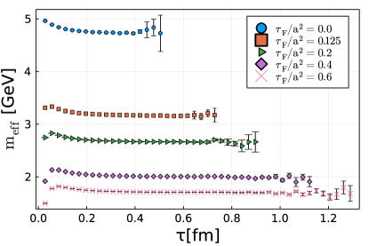
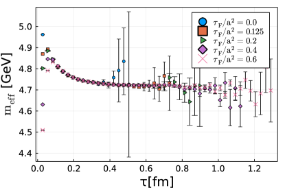
Figure 4: The effective masses corresponding to the Wilson line correlators at $r/a=15$, $\beta=8.249$ obtained for different flow times (top). The effective masses for different flow times after applying the additive shift are discussed in the text (bottom).

In Fig. 4 (top) we show the un-renormalized effective masses at $T=0$ for $\beta=8.249$ at different flow times. The improvement in the signal with increasing signal at large $\tau$ is obvious from the figure. We also see that the effective masses decrease with increasing flow time as one would expect based on the discussions above. There is a non-monotonic behavior of the effective masses in $\tau$ for $\tau/a=1-3$. This is due to the fact that the gradient flow distorts short distance physics and potentially can lead to non-positive definite spectral function for very large $\omega$. However, for not too large $\omega$ there is no sign of positivity violation in the spectral function since the effective masses approach plateaus from above for $\tau/a>3$. This means that the gradient flow does not lead to artifacts in the determination of the $Q\bar{Q}$ potential at $T=0$. By shifting the effective masses for different $\tau_{F}$ by a constant it is possible to collapse them to one line, except for very small $\tau$, where there are $\tau_{F}$-dependent distortions due to gradient flow. This is demonstrated in Fig. 4 (bottom). We determine this shift by fitting the difference in the effective masses calculated at different flow times to a constant for $\tau/a=7-18$ for $\beta=8.249$ and $\tau/a=7-15$ for the two smaller values of $\beta$. This constant shift should amount to the difference in the additive normalization of the $Q\bar{Q}$ potential, and therefore, should be independent of $Q\bar{Q}$ separation, $r$, apart from the distortions at small $r$ due to smearing. In Fig. 5 we show the relative shifts as a function of $r$ for $\beta=8.249$ We see that for very small $r$ there is some dependence on the value of $r$. This dependence becomes stronger for larger $\tau_{F}$ as there are more short distance distortions with increasing $\tau_{F}$. We obtain similar results for these additive shifts for $\beta=7.596$ and $\beta=7.825$. For all three $\beta$ values we find that for $\tau_{F}/a^{2}=0.125-0.2$ there is no dependence of this additive shift on $r$ for $r/a\geq 5$ within errors, while for larger flow times we find that there is no statistically significant $r$ dependence for $r/a\geq 7$. This means that the short distance distortions in the $Q\bar{Q}$ potential are negligible for $r/a\geq 5$ when $\tau_{F}/a^{2}\leq 0.2$, or for $r/a\geq 7$ when $\tau_{F}/a^{2}\geq 0.4$. After determining the relative shifts for different flow times, including $\tau_{F}=0$ we applied the normalization constant for the unsmeared case discussed above to determine the renormalized $T=0$ potential for different $\tau_{F}$. We compared these with the previously published results for $\beta=7.825$ and found nice agreement within errors except for very small values of $r/a$ where distortions due to gradient flow are significant.

Figure 5: The additive shifts for different flow times as a function of $r/a$ for $\beta=8.249$.

In addition to the gradient flow, we use polynomial interpolations to reduce fluctuations in the Wilson line correlators. For fixed $\tau$ the Wilson line correlators should be a smooth function of $r$ apart from the effects of breaking of rotational symmetry on the lattice. For Symanzik gauge action these effects are smaller than the statistical errors for $r/a>3$ [31, 27]. Therefore, it is natural to require that the data on the Wilson line correlators are smooth functions of $r$ at a fixed value of $\tau$. By imposing this requirement we effectively reduce the fluctuations in the original data set since nearby $r$ values usually correspond to very different path geometries and thereby suffer from quite independent gauge noise. We perform second order polynomial interpolations in a limited range of distances, $\Delta r$ around a target value of $r$ and replace the original datum with the interpolated value. We take into account that, with increasing distance, there are many different separations that are close to the target value of $r$ and adjust $\Delta r$ as we vary $r$. This additional noise reduction and the interpolation procedure are demonstrated in Fig. 6. In fact the result on the effective masses shown in Fig. 4 also incorporate the noise reduction from the interpolations.

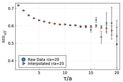
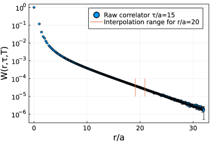
Figure 6: (top) Effective mass for $N_{\tau}=32$, $N_{x}=64$, $r/a=20$ and $\tau_{F}/a^{2}=0.125$ for the raw data, compared to an interpolation fit done around $r/a=20$ in a range $\pm\Delta r/a=0.9$ with a second order polynomial. (bottom) The correlator as a function of distance r at fixed $\tau=15a$ for the same lattice as the top plot.

Because of the use of the above noise reduction the determination of the $Q\bar{Q}$ potential at zero temperature is now more accurate. Therefore, we re-calibrated the central value of the constant $c_{Q}$ and used the following values in the present analysis: $c_{Q}(\beta=7.596)=0.3552$, $c_{Q}(\beta=7.825)=0.3401$ and $c_{Q}(\beta=8.249)=0.3135$. These values agree with the one quoted above within errors.

III Analysis of the Wilson line correlators at $T>0$

Our aim is to gain information on the spectral function corresponding to the Wilson line correlator at $T>0$. Following Ref. [10] we choose the Ansatz for the spectral function as

$$\rho_{r}(\omega,T)=\rho_{r}^{\text{low}}(\omega,T)+\rho_{r}^{\text{peak}}(\omega,T)+\rho_{r}^{\text{high}}(\omega),$$ (5)

where $\rho_{r}^{\text{high}}(\omega)$ is the dominant part of the spectral function at large $\omega$ and is assumed to be temperature independent. Furthermore, $\rho_{r}^{\text{peak}}(\omega,T)$ describes the dominant peak in the spectral function and encodes the complex potential at $T>0$, while $\rho_{r}^{\text{low}}$ is a small contribution to the spectral function below the dominant peak, which is discussed below in more detail. The position and width of the dominant peak in the spectral function should not depend on the interpolating operator details used in the static $Q\bar{Q}$ correlator, e.g. on the flow time and whether we use Wilson line correlators in Coulomb gauge or Wilson loops. On the other hand $\rho_{r}^{\text{low}}(\omega,T)$ and $\rho_{r}^{\text{high}}(\omega)$ will depend on the specific choices of the interpolating operators used in the correlator, e.g. on the amount of smearing or the gauge tolerance used. In Fig. 7 we show the effective masses for $T=305$ MeV and $r=0.606$ fm for different flow times. We see non-monotonic behavior and flow time dependence for small $\tau$ as we do for the $T=0$ case. However, for an intermediate $\tau$-range $0.1\leavevmode\nobreak\ {\rm fm}<\tau<0.45$ fm, where the contribution from $\rho_{r}^{\text{peak}}(\omega,T)$ is the dominant one, the effective masses for different flow times agree with each other very well. At $\tau>0.5$ fm the contribution from $\rho_{r}^{\text{low}}(\omega,T)$ becomes important, and we see some dependence on the flow time. As discussed in Ref. [10] $\rho_{r}^{\text{low}}(\omega,T)$ depends on the overlap of the chosen $Q\bar{Q}$ operator with the light states that propagate backward in the Euclidean time together with the forward propagating $Q\bar{Q}$. Similar dependence on the level of spatial link smearing of the effective mass was observed in Ref. [10].

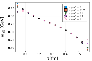
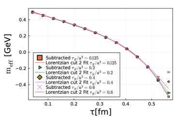
Figure 7: The effective masses for different flow times at $T=305$ MeV, $r=0.606$ fm, $\beta=7.825$. The bottom panel shows the effective masses for the subtracted correlator. The lines in the bottom panel show the fits discussed in the text.

Since the effective masses show similar behavior at small $\tau$ at $T=0$ or at $T>0$ we would like to constrain $\rho_{r}^{\text{high}}(\omega)$ by using the $T=0$ results on the Wilson line correlator. Fixing $\rho_{r}^{\text{high}}(\omega)$ to its value at zero temperature effectively means subtracting it from the finite temperature result. We define the subtracted correlator as follows:

$$W^{\text{sub}}(\tau,r,T)=W(\tau,r,T)-W^{\text{high}}(\tau,r),$$ (6)

where $W^{\text{high}}(\tau,r)$ is defined in Eq. (3). The subtracted correlator is solely determined by the medium dependent part of the spectral function $\rho_{r}^{\rm med}(\omega,T)=\rho_{r}(\omega,T)-\rho_{r}^{\rm high}(\omega)$. Since the $T=0$ spectral function has the form

$$\rho_{r}(\omega,T=0)=A_{r}\delta(\omega-V(r,T=0))+\rho_{r}^{\text{high}}(\omega),$$ (7)

we can also write

$$W^{\text{high}}(\tau,r)=W(\tau,r,T=0)-A_{r}e^{-V(r,T=0)r}.$$ (8)

Therefore, using the results from the single exponential fits for $A_{r}$ and $V(r,T=0)$ it is straightforward to estimate $W^{\text{high}}(\tau,r)$. The task of constraining $\rho_{r}^{\text{peak}}(\omega,T)$ and $\rho_{r}^{\text{low}}(\omega,T)$ is now reduced to the analysis of the $\tau$-dependence of $W^{\text{sub}}(\tau,r,T)$. As discussed in the main text the effective masses corresponding to $W^{\text{sub}}(\tau,r,T)$ decrease monotonically with $\tau$, and for sufficiently small $\tau$ they are approximately linear in $\tau$. This is demonstrated in Fig. 7, where the effective masses from $W^{\text{sub}}(\tau,r,T)$ are shown for $T=305$ MeV and $r=0.606$ fm. Thus the removal of the high energy part of the spectral function also removes the artifacts induced by the gradient flow. The linear behavior of the effective masses in $\tau$ for small $\tau$ can be easily explained if $\rho_{r}^{\text{peak}}(\omega,T))$ has a Gaussian form $\rho_{r}^{\text{G}}(\omega,T)\sim e^{-(\omega-V(r,T))^{2}/(2\Gamma_{G}^{2})}$ and the contribution from $\rho_{r}^{\text{low}}(\omega,T))$ is small

$$W^{\text{sub}}(\tau,r,T) \sim\int d\omega e^{-\omega\tau}\rho_{r}^{\text{G}}(\omega,T)$$

$$\sim\exp(-V(r,T)\tau+\frac{\Gamma_{G}^{2}}{2}\tau^{2}).$$ (9)

However, the Gaussian form of the spectral function is not physically motivated and the width of the Gaussian cannot be interpreted as ${\rm Im}V(r,T)$. If we assume that the detailed shape of the spectral function away from the peak position is not too important we can define the ${\rm Im}V(r,T)$ as the width at half maximum height. In this case, a Gaussian form of the spectral function can be used. A physically appealing choice of $\rho_{r}^{\text{peak}}(\omega,T)$ is a Lorentzian form. However, this form is only valid for $\omega$ values that are not too far from $\omega={\rm Re}V(r,T)$. The HTL spectral function of static $Q\bar{Q}$ [16] is Lorentzian only in the vicinity of the peak and decays exponentially when $|{\rm Re}V-\omega|$ is larger [16]. The same holds for the spectral function in the T-matrix approach [15]. Therefore, we use a cut Lorentzian for $\rho_{r}^{\text{peak}}(\omega,T)$ in our analysis

$$\rho_{r}^{\text{cL}}(\omega)=\frac{1}{\pi}\frac{A_{r}\Gamma_{L}\theta(\text{Cut}-|\omega-{\rm Re}V|)}{(\omega-{\rm Re}V)^{2}+\Gamma_{L}^{2}}.$$ (10)

It turns out that the cut Lorentzian also gives an almost linear dependence in $\tau$ for the effective masses. In our analysis, we set $\text{Cut}=2\Gamma_{L}$. To cross-check our results we also use the Gaussian form.

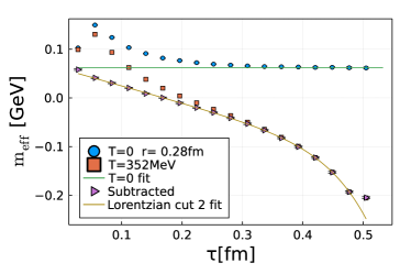
Figure 8: The effective masses for $\beta=8.249$, $T=352$ MeV, $r=0.280$ fm and the corresponding fits with the cut Lorentzian plus the delta function for $\rho_{r}^{\text{low}}$ shown as line. The bottom panel shows the relative deviation between the fit and the data with the lines indicating the estimated $1-\sigma$ band of the data.

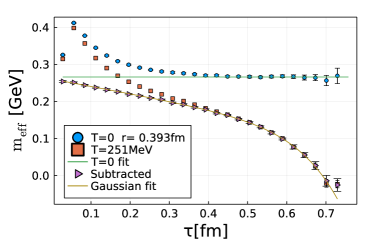
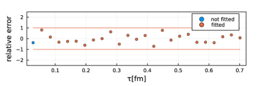
Figure 9: The effective masses for $\beta=8.249$, $T=251$ MeV, $r=0.392$ fm and the corresponding fits with the cut Lorentzian plus the delta function for $\rho_{r}^{\text{low}}$ shown as line. The bottom panel shows the relative deviation between the fit and the data with the lines indicating the estimated $1-\sigma$ band of the data.

It was shown in Ref. [10] that the rapid non-linear decrease in the effective masses is due to $\rho_{r}^{\text{low}}(\omega,T)$. This contribution to the spectral function arises from the light states in the medium propagating backward in time which are coupled to the static $Q\bar{Q}$ propagating forward in time [10]. This contribution also depends on the details of the $Q\bar{Q}$ correlators, e.g. whether one uses Wilson line or Wilson loops and the amount of smearing used [10]. We model this part of the spectral function with a single delta function because such a simple form is sufficient to describe the data for the Wilson line correlators with the exception of one data point very close to the boundary $\tau=1/T$. We perform fits of subtracted Wilson line correlator with Lorentzian form of $\rho_{r}^{\text{peak}}(\omega,T)$ and a single delta function for $\rho_{r}^{\text{low}}(\omega,T)$ for all available data sets omitting the first datum, which is possibly affected by the distortions due to smearing, and the last data point. Some sample fits are shown in Fig. 7 for $T=305$ MeV, $r=0.606$ fm, $\beta=7.825$, and in Fig. 8 for $T=352$ MeV, $r=0.28$ fm, $\beta=8.249$. The fits work well as demonstrated in Fig. 8 (bottom), where the relative difference between the fit and the lattice data is shown. Fits using the Gaussian form for $\rho_{r}^{\text{peak}}(\omega,T)$ work equally well as demonstrated in Fig. 9.

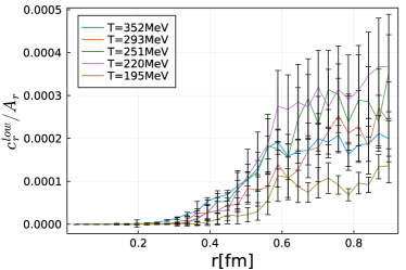
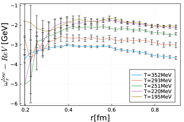
Figure 10: The amplitude of the small delta function divided by $A_{r}$ (left) and the position of the small delta function relative to the position of the dominant peak (right) as a function of $r$. The results are shown at different temperatures for lattice spacing $a=0.0280$ fm ($\beta=8.249$).

The amplitude and the position of the small delta function that parametrizes $\rho_{r}^{\rm low}$ are shown relative to the dominant peak in Fig. 10 for $\beta=8.249$ and different temperatures. As one can see from the figure the position of this delta function is between $1.8$ GeV and 3.8 GeV below the position of the dominant peak, and shows only mild dependence on $r$. The amplitude of this delta function on the other hand increases rapidly with increasing $r$. Similar results have been obtained for the two other $\beta$ values. We also note that for small values of $r$, typically smaller than five times the lattice spacing, it is not necessary to include this small delta function in the fits, i.e. we can set $\rho_{r}^{\rm low}$ to zero and obtain good fits.

In Fig. 11 we show the width of spectral function defined as the width at half of the maximum height as a function of $r$ and different temperatures obtained from the fits using Gaussian and Lorentzian form for $\rho_{r}^{\text{peak}}(\omega,T)$. We see that using the Gaussian results in a systematically larger width. The Lorentzian parameter $\Gamma_{L}$ though is dependent on the cut on the Lorentzian. This means that there is a systematic uncertainty in the determination of ${\rm Im}V(r,T)$ from the parametrization of the spectral function. As we discuss in the section below it is possible to define the width in a model independent way by considering cumulants of the spectral function.

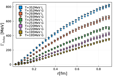
Figure 11: Width at half the maximum height (FWHM) for the Lorentzian cut fit and Gaussian fit.

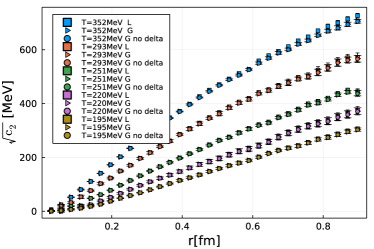
Figure 12: $\sqrt{c_{2}}$ for the Gaussian fit (G), compared to the Lorentzian fit (L), or to a Gaussian fit without accounting for the low $\omega$ structure (G no delta).

IV Cumulants of the spectral function

The cumulants of the spectral functions $c_{n}$ are defined as

$$c_{1} =\langle\omega\rangle,$$ (11)

$$c_{2} =\langle\omega^{2}\rangle-\langle\omega\rangle^{2},$$ (12)

$$c_{3} =\langle\omega^{3}\rangle-3\langle\omega\rangle\langle\omega^{2}\rangle+2\langle\omega\rangle^{3},$$ (13)

where $\langle...\rangle$ stands for $\int d\omega\rho_{r}(\omega,T)...$. Cumulants exist if the spectral function has support in a finite $\omega$ range, which is the case for the subtracted spectral function $\rho_{r}^{\rm sub}(\omega,T)=\rho_{r}(\omega,T)-\rho_{r}^{\rm high}(\omega)\equiv\rho_{r}^{\text{med}}(\omega,T)$. In what follows we will discuss the moments of this spectral function. The cumulants of the spectral function are related to the cumulants of the subtracted Wilson line correlators at $\tau=0$, $m_{n}$ defined as

$$W^{\rm sub}(\tau,r,T)=\exp\Bigg{[}\sum_{n=0}^{\infty}\frac{m_{n}(-\tau)^{n}}{n!}\Bigg{]}$$ (14)

This can be seen by Taylor expanding the exponential in the spectral representation of the subtracted Wilson line correlator

$$W^{\rm sub}(\tau,r,T) =\int d\omega e^{-\omega\tau}\rho_{r}^{\text{sub}}(\omega,T)$$

$$=\int d\omega\sum_{n=0}^{\infty}\frac{(-\omega\tau)^{n}}{n!}\rho_{r}^{\text{sub}}(\omega,T)$$

$$=\sum_{n=0}^{\infty}\langle\omega^{n}\rangle\frac{(-\tau)^{n}}{n!}$$ (15)

Expanding the exponential in Eq. (14) and comparing to Eq. (15) we see that:

$$m_{1} =\langle\omega\rangle,$$ (16)

$$m_{2} =\langle\omega^{2}\rangle-\langle\omega\rangle^{2}.$$ (17)

The first cumulant of the Wilson line correlators is the effective mass. The second cumulant is the slope of the effective mass in $\tau$.

We calculated the second cumulant of the subtracted spectral function using the Gaussian form and cut Lorentzian form including and excluding the $\delta$ function at small $\omega$. The result of this analysis is shown in Fig. 12. We see that the second cumulant of the spectral function is not sensitive whether we use a Gaussian or cut Lorentzian in our analysis. Furthermore, the second cumulant does not change much if we include or exclude the contribution from $\rho_{r}^{\text{low}}$ that is the small delta peak. We also see that $\sqrt{c_{2}}$ has a similar dependence on $r$ as the width parameter shown in Fig. 11 but is somewhat smaller.

We can also fit our lattice results on the subtracted Wilson line correlator with the following simple form

$$W^{\text{approx}}(\tau,r,T)=\exp(m_{0}-m_{1}\tau+m_{2}\tau^{2}/2)$$ (18)

in the range $\tau/a=2-N_{\tau}/3$, where the effective mass is approximately linear. From this fit, we can then estimate the second cumulant of the spectral function and compare it with the determination of $c_{2}$ obtained by integrating the model spectral function based on the cut Lorentzian and the small delta function in the almost entire $\tau$ range. This comparison is shown in Fig. 13. We see that the two methods of estimating $c_{2}$ are in good agreement. This means that defining ${\rm Im}V(r,T)$ in terms of $c_{2}$ is model independent and robust.

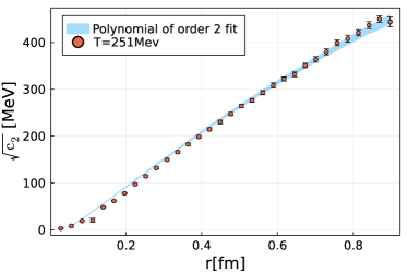
Figure 13: The second cumulant of the subtracted spectral function as a function of $r$ determined from the cut Lorentzian form of the spectral function (circles) and from the second order polynomial fit of the Wilson line correlation function in the $\tau/a$ range $2-N_{\tau}/3$ (blue band) for $T=251$ MeV and $a=0.0280$ fm.

We also calculated the third cumulant of the spectral function using our fitted spectral function based on the cut Lorentzian form. The result on $c_{3}$, which is the measure of skewness of the spectral function, is shown in Fig. 14. We see that $-c_{3}$ is close to zero at small $r$ but then rapidly increases with increasing $r$. For very small distances, $r<5a$ $\rho_{r}^{\rm low}$ was not included in the fit, and therefore, $c_{3}$ is exactly zero here. Unfortunately, our lattice results are not precise enough to obtain $c_{3}$ using fits with Eq. (18) extended to higher order polynomials in the exponent. Thus at the present level of accuracy, the short $\tau$ behavior of the effective masses can be parametrized solely by $m_{1}$ and $m_{2}$.

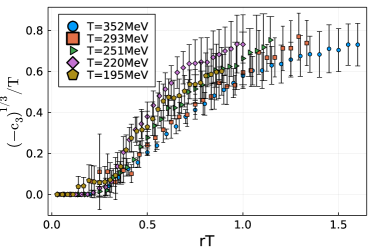
Figure 14: $(-c_{3})^{1/3}$ as a function of $r$ in temperature units for lattice spacing $a=0.0280$ fm and different temperatures.

References

- Busza et al. [2018] W. Busza, K. Rajagopal, and W. van der Schee, Heavy Ion Collisions: The Big Picture, and the Big Questions, Ann. Rev. Nucl. Part. Sci. 68, 339 (2018), arXiv:1802.04801 [hep-ph] .
- Matsui and Satz [1986] T. Matsui and H. Satz, Suppression by Quark-Gluon Plasma Formation, Phys. Lett. B178, 416 (1986).
- Zhao et al. [2020] J. Zhao, K. Zhou, S. Chen, and P. Zhuang, Heavy flavors under extreme conditions in high energy nuclear collisions, Prog. Part. Nucl. Phys. 114, 103801 (2020), arXiv:2005.08277 [nucl-th] .
- Bazavov and Weber [2021] A. Bazavov and J. H. Weber, Color Screening in Quantum Chromodynamics, Prog. Part. Nucl. Phys. 116, 103823 (2021), arXiv:2010.01873 [hep-lat] .
- Laine et al. [2007] M. Laine, O. Philipsen, P. Romatschke, and M. Tassler, Real-time static potential in hot QCD, JHEP 03, 054, arXiv:hep-ph/0611300 [hep-ph] .
- Brambilla et al. [2008] N. Brambilla, J. Ghiglieri, A. Vairo, and P. Petreczky, Static quark-antiquark pairs at finite temperature, Phys. Rev. D78, 014017 (2008), arXiv:0804.0993 [hep-ph] .
- Rothkopf et al. [2012] A. Rothkopf, T. Hatsuda, and S. Sasaki, Complex Heavy-Quark Potential at Finite Temperature from Lattice QCD, Phys. Rev. Lett. 108, 162001 (2012), arXiv:1108.1579 [hep-lat] .
- Bala and Datta [2020] D. Bala and S. Datta, Nonperturbative potential for the study of quarkonia in QGP, Phys. Rev. D 101, 034507 (2020), arXiv:1909.10548 [hep-lat] .
- Burnier et al. [2015] Y. Burnier, O. Kaczmarek, and A. Rothkopf, Quarkonium at finite temperature: Towards realistic phenomenology from first principles, JHEP 12, 101, arXiv:1509.07366 [hep-ph] .
- Bala et al. [2022] D. Bala, O. Kaczmarek, R. Larsen, S. Mukherjee, G. Parkar, P. Petreczky, A. Rothkopf, and J. H. Weber (HotQCD), Static quark-antiquark interactions at nonzero temperature from lattice QCD, Phys. Rev. D 105, 054513 (2022), arXiv:2110.11659 [hep-lat] .
- Follana et al. [2007] E. Follana, Q. Mason, C. Davies, K. Hornbostel, G. P. Lepage, J. Shigemitsu, H. Trottier, and K. Wong (HPQCD, UKQCD), Highly improved staggered quarks on the lattice, with applications to charm physics, Phys. Rev. D75, 054502 (2007), arXiv:hep-lat/0610092 [hep-lat] .
- Luscher and Weisz [1985a] M. Luscher and P. Weisz, On-Shell Improved Lattice Gauge Theories, Commun. Math. Phys. 97, 59 (1985a), [Erratum: Commun.Math.Phys. 98, 433 (1985)].
- Luscher and Weisz [1985b] M. Luscher and P. Weisz, Computation of the Action for On-Shell Improved Lattice Gauge Theories at Weak Coupling, Phys. Lett. B 158, 250 (1985b).
- Lüscher [2010] M. Lüscher, Properties and uses of the Wilson flow in lattice QCD, JHEP 08, 071, [Erratum: JHEP 03, 092 (2014)], arXiv:1006.4518 [hep-lat] .
- Liu and Rapp [2018] S. Y. F. Liu and R. Rapp, -matrix Approach to Quark-Gluon Plasma, Phys. Rev. C 97, 034918 (2018), arXiv:1711.03282 [nucl-th] .
- Burnier and Rothkopf [2013] Y. Burnier and A. Rothkopf, A hard thermal loop benchmark for the extraction of the nonperturbative potential, Phys. Rev. D87, 114019 (2013), arXiv:1304.4154 [hep-ph] .
- Mazur et al. [2023] L. Mazur et al., SIMULATeQCD: A simple multi-GPU lattice code for QCD calculations, (2023), arXiv:2306.01098 [hep-lat] .
- Bazavov et al. [2018a] A. Bazavov, P. Petreczky, and J. Weber, Equation of State in 2+1 Flavor QCD at High Temperatures, Phys. Rev. D 97, 014510 (2018a), arXiv:1710.05024 [hep-lat] .
- Bazavov et al. [2010] A. Bazavov et al. (MILC), Results for light pseudoscalar mesons, PoS LATTICE2010, 074 (2010), arXiv:1012.0868 [hep-lat] .
- Bazavov et al. [2014a] A. Bazavov et al. (HotQCD), Equation of state in ( 2+1 )-flavor QCD, Phys. Rev. D 90, 094503 (2014a), arXiv:1407.6387 [hep-lat] .
- Clark and Kennedy [2004] M. A. Clark and A. D. Kennedy, The RHMC algorithm for two flavors of dynamical staggered fermions, Nucl. Phys. B Proc. Suppl. 129, 850 (2004), arXiv:hep-lat/0309084 .
- Aubin et al. [2004] C. Aubin, C. Bernard, C. DeTar, J. Osborn, S. Gottlieb, E. B. Gregory, D. Toussaint, U. M. Heller, J. E. Hetrick, and R. Sugar, Light hadrons with improved staggered quarks: Approaching the continuum limit, Phys. Rev. D 70, 094505 (2004), arXiv:hep-lat/0402030 .
- Cheng et al. [2008] M. Cheng et al., The QCD equation of state with almost physical quark masses, Phys. Rev. D 77, 014511 (2008), arXiv:0710.0354 [hep-lat] .
- Bazavov et al. [2012] A. Bazavov et al., The chiral and deconfinement aspects of the QCD transition, Phys. Rev. D85, 054503 (2012), arXiv:1111.1710 [hep-lat] .
- Brambilla et al. [2023] N. Brambilla, R. L. Delgado, A. S. Kronfeld, V. Leino, P. Petreczky, S. Steinbeißer, A. Vairo, and J. H. Weber (TUMQCD), Static energy in ()-flavor lattice QCD: Scale setting and charm effects, Phys. Rev. D 107, 074503 (2023), arXiv:2206.03156 [hep-lat] .
- Hasenfratz and Knechtli [2001] A. Hasenfratz and F. Knechtli, Flavor symmetry and the static potential with hypercubic blocking, Phys. Rev. D 64, 034504 (2001), arXiv:hep-lat/0103029 .
- Bazavov et al. [2019] A. Bazavov, N. Brambilla, X. Garcia i Tormo, P. Petreczky, J. Soto, A. Vairo, and J. H. Weber (TUMQCD), Determination of the QCD coupling from the static energy and the free energy, Phys. Rev. D 100, 114511 (2019), arXiv:1907.11747 [hep-lat] .
- Ramos and Sint [2016] A. Ramos and S. Sint, Symanzik improvement of the gradient flow in lattice gauge theories, Eur. Phys. J. C 76, 15 (2016), arXiv:1508.05552 [hep-lat] .
- Hoying et al. [2022] D. Hoying, A. Bazavov, D. Bala, G. Parkar, O. Kaczmarek, R. Larsen, S. Mukherjee, P. Petreczky, A. Rothkopf, and J. H. Weber, Static potential at non-zero temperatures from fine lattices, PoS LATTICE2021, 178 (2022), arXiv:2110.00565 [hep-lat] .
- Bazavov et al. [2018b] A. Bazavov, N. Brambilla, P. Petreczky, A. Vairo, and J. H. Weber (TUMQCD), Color screening in (2+1)-flavor QCD, Phys. Rev. D 98, 054511 (2018b), arXiv:1804.10600 [hep-lat] .
- Bazavov et al. [2014b] A. Bazavov, N. Brambilla, X. Gacia i Tormo, P. Petreczky, J. Soto, and A. Vairo, Determination of from the QCD static energy: An update, Phys. Rev. D 90, 074038 (2014b), [Erratum: Phys.Rev.D 101, 119902 (2020)], arXiv:1407.8437 [hep-ph] .