Highest Cusped Waves for the Fractional KdV Equations

Abstract

In this paper we prove the existence of highest, cusped, traveling wave solutions for the fractional KdV equations $f_{t}+ff_{x}=|D|^{\alpha}f_{x}$ for all $\alpha\in(-1,0)$ and give their exact leading asymptotic behavior at zero. The proof combines careful asymptotic analysis and a computer-assisted approach.

1 Introduction

This paper is concerned with the existence and regularity of highest, cusped, periodic traveling-wave solutions to the fractional Korteweg-de Vries (KdV) equations, in the periodic setting given by

$$f_{t}+ff_{x}=|D|^{\alpha}f_{x},\quad\text{ for }(x,t)\in\mathbb{T}\times\mathbb{R}.$$ (1)

Here $|D|^{\alpha}$ is the Fourier multiplier operator given by

$$\widehat{|D|^{\alpha}f}(\xi)=|\xi|^{\alpha}\widehat{f}(\xi)$$

where the parameter $\alpha$ may in general take any real value. It can serve as a model for investigating the balance between nonlinear and dispersive effects [47]. For $\alpha=2$ and $\alpha=1$ it reduces to the classical KdV and Benjamin-Ono equations, for $\alpha=-2$ one gets the reduced Ostrovsky equation. For $\alpha=-1$ it reduces to the Burgers-Hilbert equation [31]

$$f_{t}+ff_{x}=\mathbf{H}[f],\quad\text{ for }(x,t)\in\mathbb{T}\times\mathbb{R}.$$ (2)

Here $\mathbf{H}$ is the Hilbert transform which, for $f:\mathbb{T}\to\mathbb{R}$, is defined by

$$\mathbf{H}[f](x)=\frac{1}{2\pi}p.v.\int_{-\pi}^{\pi}\cot\left(\frac{x-y}{2}\right)f(y)\ dy,\quad\widehat{\mathbf{H}[f]}(k)=-i\operatorname{sgn}(k)\widehat{f}(k).$$

The results in this paper, see Theorem 1.1, are for $\alpha\in(-1,0)$, though the analysis of the Burgers-Hilbert case, $\alpha=-1$, is also important for the proof.

For $\alpha\in(-1,0)$ and small initial data in $H^{N}(\mathbb{R})$ with $N\geq 3$ estimates for the life span were proved by Ehrnström and Wang [21], see also [32] and [33] for the Burgers-Hilbert equation. Well-posedness in $H^{s}(\mathbb{R})$ with $s>3/2$ was established by Riaño [52].

For $\alpha\in(-1,0)$ the equation exhibits finite time blow [8, 34]. The characterization as wave breaking (i.e. the functions stay bounded, but its gradient blows up) was proved for $\alpha\in(-1,-1/3)$ by Hur and Tao [36, 35] and for $\alpha\in(-1,0)$ by Oh and Pasqualotto [50]. See [45] for a numerical study and [13] where they give a precise characterization of a chock forming in finite time for $0<\alpha<\frac{1}{3}$.

The study of traveling waves is an important topic in fluid dynamics, see e.g. [29] for a recent overview of traveling water waves. The traveling wave assumption $f(x,t)=\varphi(x-ct)$, where $c>0$ denotes the wave speed, gives us

$$-c\varphi^{\prime}+\varphi\varphi^{\prime}=|D|^{\alpha}\varphi^{\prime}.$$ (3)

For the fractional KdV equation there is a branch of even, zero-mean, $2\pi$-periodic, smooth traveling wave solutions bifurcating from constant solutions. For $\alpha<-1$ and $\alpha\in(-1,0)$ this branch has been studied and proved to end in a highest cusped wave, for $\alpha<-1$ by Bruell and Dhara [6] and for $\alpha\in(-1,0)$ by Hildrum and Xue [30]. For $\alpha=-1$ the branch has been studied by Castro, Córdoba and Zheng [9].

The notion of a highest traveling wave goes back to Stokes. For the free boundary Euler equation Stokes argued that if there exists a singular solution with a steady profile it must have an interior angle of $120^{\circ}$ at the crest [53]. This is known as the Stokes conjecture and was proved in 1982 [1]. For the Whitham equation [56] the existence of a highest cusped traveling wave was conjectured by Whitham in [55]. Its existence, together with its $C^{1/2}$ regularity, was proved by Ehrnström and Wahlén [20]. For the family of fractional KdV equation and variants thereof there has recently been much progress related to highest waves. Bruell and Dhara proved existence of highest traveling waves which are Lipschitz at their cusp for $\alpha<-1$ [6]. Hildrum and Xue proved existence and the optimal $-\alpha$-Hölder regularity for a family of equations including the fractional KdV equation with $\alpha\in(-1,0)$ [30]. Ørke proved their existence for $\alpha\in(-1,0)$ for the inhomogeneous fractional KdV equations as well as the fractional Degasperis-Procesi equations, together with their optimal $-\alpha$-Hölder regularity [51].

The results in [20, 6, 51, 30] are all based on global bifurcation arguments, bifurcating from the constant solution and proving that the branch must end in a highest wave which is not smooth at its crest. For the Burgers-Hilbert equation Dahne and Gómez-Serrano proved the existence of a highest wave which at its cusp behaves like $|x|\log|x|$ [15]. The proof uses a different method where the problem is first reduced to a fixed point problem. The wave is therefore not directly tied to a branch of solutions as in the other results. This method of rewriting the problem into a fixed point problem was first used by Enciso, Gómez-Serrano and Vergara for proving the convexity and the precise asymptotic behavior of a highest wave solution to the Whitham equation [22], answering a conjecture made by Ehrnström and Wahlén [20]. In this paper we use a similar approach.

Similar to Hildrum and Xue we prove the existence of a highest wave for the fractional KdV equation with $\alpha\in(-1,0)$. Our main contribution is a more precise description of the asymptotic behavior of the wave at the cusp. The description is in line with earlier results for the Whitham and Burgers-Hilbert equation. Recently Ehrnström, Mæhlen and Varholm have obtained similar results for the asymptotic behavior of two families of equations including the uni- and bidirectional Whitham equations using different types of methods [19].

We prove the following theorem:

Theorem 1.1.

There is a $2\pi$-periodic traveling wave $\varphi$ of (3) for every $\alpha\in(-1,0)$, which behaves asymptotically at $x=0$ as

$$\varphi(x)=c-\nu_{\alpha}|x|^{-\alpha}+\mathcal{O}(|x|^{p}).$$

for $\nu_{\alpha}>0$ as given in Lemma 4.1 and some $-\alpha<p\leq 1$ to be made explicit later on.

Remark 1.2.

The remainder term $\mathcal{O}(|x|^{p})$ in Theorem 1.1 is in general not sharp. The estimate follows from the choice of our space.

Remark 1.3.

Both our results and Hildrum and Xue’s results assert the existence of a highest wave. While, a priori, they don’t necessarily correspond to the same wave, we do believe this is the case.

The ansatz $\varphi(x)=c-u(x)$ allows us to rewrite (3) as an equation that does not explicitly depend on the wave speed $c$. Proving the existence of a solution $u$ can be rewritten as a fixed point problem by considering the ansatz

$$u(x)=u_{\alpha}(x)+w_{\alpha}(x)v(x)$$

where $u_{\alpha}(x)$ is an explicit, carefully chosen, approximate solution and $w_{\alpha}(x)$ is an explicit weight factor. Proving the existence of a fixed point can be reduced to checking an inequality involving three constants, $D_{\alpha}$, $\delta_{\alpha}$ and $n_{\alpha}$, that only depend on the choice of $u_{\alpha}$ and $w_{\alpha}$, see Proposition 2.2. This inequality is checked by bounding $D_{\alpha}$, $\delta_{\alpha}$ and $n_{\alpha}$ using a computer-assisted proof, see Section 12.

One of the key difficulties compared to the Whitham equation [22] and the Burgers-Hilbert equation [15] is that we are treating a family of equations, instead of one fixed equation. To handle the full family we need to understand how the equation changes with respect to $\alpha$. In particular the endpoints of the interval, $\alpha$ near $-1$ and $0$, require adapting the method to those cases. To handle this we split the interval $(-1,0)$ into three parts,

$$(-1,0)=(-1,-1+\delta_{1})\cup[-1+\delta_{1},-\delta_{2}]\cup(-\delta_{2},0)=I_{1}\cup I_{2}\cup I_{3},$$

and adapt the methods used for $I_{1}$ and $I_{3}$. For $\alpha\in I_{1}$ the main complication comes from that as $\alpha\to-1$ the coefficient $\nu_{\alpha}$ in Theorem 1.1 tends to infinity. For $\alpha\in I_{3}$ the issue is that both sides of the inequality that needs to be verified for the fixed point argument tend to zero as $\alpha\to 0$ and to assert that it holds arbitrarily close to $\alpha=0$ we need an understanding of the rate at which the two sides tend to zero.

An important part of the work is the construction of the approximate solution $u_{\alpha}$. Due to the singularity at $x=0$ it is not possible to use a trigonometric polynomial alone, it would converge very slowly and have the wrong asymptotic behavior. Pure products of powers and logarithms, $|x|^{a}\log^{b}|x|$, have the issue that they are not periodic and do not interact well with the operator $|D|^{\alpha}$. Instead we take inspiration from the construction in [22] and consider a combination of trigonometric polynomials and Clausen functions of different orders, defined as

$$C_{s}(x)=\sum_{n=1}^{\infty}\frac{\cos(nx)}{n^{s}},\quad S_{s}(x)=\sum_{n=1}^{\infty}\frac{\sin(nx)}{n^{s}},$$

for $s>1$ and by analytic continuation otherwise. We also make use of their derivatives with respect to the order, for which we use the notation

$$C_{s}^{(\beta)}(x):=\frac{d^{\beta}}{ds^{\beta}}C_{s}(x),\quad S_{s}^{(\beta)}(x):=\frac{d^{\beta}}{ds^{\beta}}S_{s}(x).$$

The Clausen functions are $2\pi$-periodic, non-analytic at $x=0$ and behave well with respect to $|D|^{\alpha}$. In particular $C_{s}(x)-C_{s}(0)\sim|x|^{s-1}$, which corresponds to the behavior we expect in Theorem 1.1. See Section 3 and Appendix C for more details about the Clausen functions. The main idea for the construction is the same as in [22], to choose the coefficients for the Clausen functions according to the asymptotic expansion of the solution at $x=0$. However, in our case we also have to handle the limits $\alpha\to-1$ and $\alpha\to 0$, which requires a good understanding of how the approximations depend on $\alpha$. In particular understanding the limit $\alpha\to-1$ is important not only for this work, but is also used to handle the Burgers-Hilbert case in [15].

An essential part of our work is the interplay between traditional mathematical tools and rigorous computer calculations. Traditional numerical methods typically only compute approximate results, to be able to use the results in a proof we need the results to be rigorously verified. The basis for rigorous calculations is interval arithmetic, pioneered by Moore in the 1970s [49]. Due to improvements in both computational power and great improvements in software it is getting practical to use computer-assisted tools in more and more complicated settings. The main idea with interval arithmetic is to do arithmetic not directly on real numbers but on intervals with computer representable endpoints. Given a function $f:\mathbb{R}\to\mathbb{R}$, an interval extension of $f$ is an extension to intervals satisfying that for an interval $\textbf{{x}}=[\underline{x},\overline{x}]$, $f(\textbf{{x}})$ is an interval satisfying $f(x)\in f(\textbf{{x}})$ for all $x\in\textbf{{x}}$. In particular this allows us to prove inequalities for the function $f$, for example the right endpoint of $f(\textbf{{x}})$ gives an upper bound of $f$ on the interval x. For an introduction to interval arithmetic and rigorous numerics we refer the reader to the books [49, 54] and to the survey [26] for a specific treatment of computer-assisted proofs in PDE. For computer-assisted proofs in fluid mechanics in particular some recent results are: [4, 2] for the Navier-Stokes equation, [23, 24, 25] for the Kuramoto-Shivasinsky equation, [12] for the Hou-Luo model, [7] for the compressible Euler and Navier-Stokes equations and [10, 11] for blowup of the 2D Boussinesq and 3D Euler equation.

For all the calculations in this paper we make use of the Arb library [41] for ball (intervals represented as a midpoint and radius) arithmetic. It has good support for many of the special functions we use [43, 37, 42], Taylor arithmetic (see e.g. [39]) as well as rigorous integration [38].

The paper is organized as follows. In Section 2 we reduce the proof of Theorem 1.1 to a fixed point problem. In Section 3 we give a brief overview of properties of the Clausen functions that are relevant for the construction of $u_{\alpha}$, in Section 4 we give the construction of $u_{\alpha}$ and in Section 5 we discuss the choice of the weight function $w_{\alpha}$ used. Section 6 gives the general strategy for bounding $n_{\alpha}$, $\delta_{\alpha}$ and $D_{\alpha}$, Section 7 and 8 discusses evaluation of $u_{\alpha}$. Section 9 is devoted to the approach for bounding $n_{\alpha}$, Section 10 to bounding $\delta_{\alpha}$ and Section 11 to studying the linear operator that appears in the construction of the fixed point problem and bounding $D_{\alpha}$. The computer-assisted proofs giving bounds for $n_{\alpha}$, $\delta_{\alpha}$ and $D_{\alpha}$ are given in Section 12. Finally we give the proof of Theorem 1.1 in Section 13.

Six appendices are given at the end of the paper. Appendix A gives some technical details for how to compute enclosures of functions around removable singularities. Appendix B gives a brief introduction to Taylor models which are used in some parts of the proof. Appendix C is concerned with computing enclosures of the Clausen functions and Appendix D with the rigorous numerical integration needed for bounding $D_{0}$. Finally Appendix E, F and G contains some of the details needed for $\alpha$ close to $-1$.

2 Reduction to a fixed point problem

In this section we reduce the problem of proving Theorem 1.1 to proving the existence of a fixed point for a certain operator.

From [30, Theorem 12] we have the following characterization of even, nondecreasing solutions of (1).

Lemma 2.1.

Let $\varphi\in C^{1}$ be a nonconstant, even solution of (1) which is nondecreasing on $(-\pi,0)$, then

$$\varphi^{\prime}>0\quad\text{ and }\quad\varphi<c$$

on $(-\pi,0)$.

As a consequence, any continuous, nonconstant, even function which is nondecreasing on $(-\pi,0)$ that satisfy (1) almost everywhere must satisfy $\varphi\leq c$. The maximal possible height is thus given by $c$ and due to the function being even and nondecreasing on $(-\pi,0)$ the maximal height has to be attained at $x=0$.

Now, the ansatz $\varphi(x)=c-u(x)$ inserted in (3) gives an equation which does not explicitly depend on the wave speed $c$. Indeed, inserting this gives us

$$uu^{\prime}=-|D|^{\alpha}u^{\prime}.$$ (4)

Note that a solution of this equation gives a solution of (3) for any wave speed $c$. This is to be expected due to the Galilean change of variables

$$\varphi\mapsto\varphi+\gamma,\ c\mapsto c+\gamma$$

which leaves (3) invariant. In particular, taking $c$ equal to the mean of $u$ gives a zero mean solution. For a highest wave we expect to have $\varphi(0)=c$, giving us $u(0)=0$. Integrating (4) gives us

$$\frac{1}{2}u^{2}=-\mathcal{H}^{\alpha}[u].$$ (5)

Here $\mathcal{H}$ is the operator

$$\mathcal{H}^{\alpha}[u](x)=|D|^{\alpha}u(x)-|D|^{\alpha}u(0).$$ (6)

It is the integral of the right-hand side of (4) with the constant of integration taken such that $\mathcal{H}^{\alpha}[f](0)=0$, this ensures that any solution of (5) satisfies $u(0)=0$. Note that any solution of (5) is a solution of (4) and hence gives a solution to (3).

To reduce the problem to a fixed point problem the idea is to write $u$ as one, explicit, approximate solution of Equation (5) and one unknown term. More precisely we make the ansatz

$$u(x)=u_{\alpha}(x)+w_{\alpha}(x)v(x)$$ (7)

where $u_{\alpha}(x)$ is an explicit, carefully chosen, approximate solution of Equation (5), see Section 4, and $w_{\alpha}(x)$ is an explicit weight, see Section 5, both of them depending on $\alpha$. By taking $u_{\alpha}(x)\sim\nu_{\alpha}|x|^{-\alpha}$ and $w_{\alpha}=\mathcal{O}(|x|^{p})$, proving Theorem 1.1 reduces to proving existence of $v\in L^{\infty}(\mathbb{T})$ such that the given ansatz is a solution of Equation (5).

Inserting the ansatz (7) into Equation (5) gives us

$$\frac{1}{2}(u_{\alpha}+w_{\alpha}v)^{2}=-\mathcal{H}^{\alpha}[u_{\alpha}+w_{\alpha}v]\iff\frac{1}{2}u_{\alpha}^{2}+u_{\alpha}w_{\alpha}v+\frac{1}{2}w_{\alpha}^{2}v^{2}=-\mathcal{H}^{\alpha}[u_{\alpha}]-\mathcal{H}^{\alpha}[w_{\alpha}v]$$

By collecting all the linear terms in $v$ we can write this as

$$u_{\alpha}w_{\alpha}v+\mathcal{H}^{\alpha}[w_{\alpha}v]=-\mathcal{H}^{\alpha}u_{\alpha}-\frac{1}{2}u_{\alpha}^{2}-\frac{1}{2}w_{\alpha}^{2}v^{2}\iff v+\frac{1}{w_{\alpha}u_{\alpha}}\mathcal{H}^{\alpha}[v]=-\frac{1}{w_{\alpha}u_{\alpha}}\left(\mathcal{H}^{\alpha}[u_{\alpha}]+u_{\alpha}^{2}\right)-\frac{w_{\alpha}}{2u_{\alpha}}v^{2}.$$

Now let $T_{\alpha}$ denote the operator

$$T_{\alpha}[v]=-\frac{1}{w_{\alpha}u_{\alpha}}\mathcal{H}^{\alpha}[w_{\alpha}v].$$ (8)

Denote the weighted defect of the approximate solution $u_{\alpha}(x)$ by

$$F_{\alpha}(x)=\frac{1}{w_{\alpha}(x)u_{\alpha}(x)}\left(\mathcal{H}^{\alpha}[u_{\alpha}](x)+\frac{1}{2}u_{\alpha}(x)^{2}\right),$$ (9)

and let

$$N_{\alpha}(x)=\frac{w_{\alpha}(x)}{2u_{\alpha}(x)}.$$ (10)

Then we can write the above as

$$(I-T_{\alpha})v=-F_{\alpha}-N_{\alpha}v^{2}.$$

Assuming that $I-T_{\alpha}$ is invertible we rewrite this as

$$v=(I-T_{\alpha})^{-1}\left(-F_{\alpha}-N_{\alpha}v^{2}\right)=:G_{\alpha}[v].$$ (11)

Hence proving the existence of $v$ such that $u_{\alpha}+w_{\alpha}v$ is a solution to Equation (5) reduces to proving existence of a fixed point of the operator $G_{\alpha}$.

Next we reduce the problem of proving that $G_{\alpha}$ has a fixed point to checking an inequality for three numbers (depending on $\alpha$) that depend only on the choice of $u_{\alpha}$ and $w_{\alpha}$. We let $\|T\|$ denote the $L^{\infty}(\mathbb{T})\to L^{\infty}(\mathbb{T})$ norm of a linear operator $T$.

Proposition 2.2.

Let $D_{\alpha}=\|T_{\alpha}\|$, $\delta_{\alpha}=\|F_{\alpha}\|_{L^{\infty}(\mathbb{T})}$ and $n_{\alpha}=\|N_{\alpha}\|_{L^{\infty}(\mathbb{T})}$. If $D_{\alpha}<1$ and they satisfy the inequality

$$\delta_{\alpha}<\frac{(1-D_{\alpha})^{2}}{4n_{\alpha}}$$

then for

$$\epsilon_{\alpha}=\frac{1-D_{\alpha}-\sqrt{(1-D_{\alpha})^{2}-4\delta_{\alpha}n_{\alpha}}}{2n_{\alpha}}$$

and

$$X_{\epsilon}=\{v\in L^{\infty}(\mathbb{T}):v(x)=v(-x),\|v\|_{L^{\infty}(\mathbb{T})}\leq\epsilon\}$$

we have

1. $G_{\alpha}(X_{\epsilon_{\alpha}})\subseteq X_{\epsilon_{\alpha}}$;

2. $\|G_{\alpha}[v]-G_{\alpha}[w]\|_{L^{\infty}(\mathbb{T})}\leq k_{\alpha}\|v-w\|_{L^{\infty}(\mathbb{T})}$ with $k_{\alpha}<1$ for all $v,w\in X_{\epsilon_{\alpha}}$.

Proof.

Using that $N_{\alpha}$ and $F_{\alpha}$ are even it can be checked that

$$G_{\alpha}(X_{\epsilon_{\alpha}})\subseteq(I-T)^{-1}X_{\delta_{\alpha}+n_{\alpha}\epsilon_{\alpha}^{2}}.$$

Since $\|T_{\alpha}\|<1$ the operator $I-T_{\alpha}$ is invertible and an upper bound of the norm of the inverse is given by $\frac{1}{1-D_{\alpha}}$, moreover $T_{\alpha}$ takes even functions to even functions and hence so will $(I-T_{\alpha})^{-1}$. This gives us

$$G_{\alpha}(X_{\epsilon_{\alpha}})\subseteq(I-T)^{-1}X_{\delta_{\alpha}+n_{\alpha}\epsilon_{\alpha}^{2}}\subseteq X_{\frac{\delta_{\alpha}+n_{\alpha}\epsilon_{\alpha}^{2}}{1-D_{\alpha}}}.$$

The choice of $\epsilon_{\alpha}$ then gives

$$\frac{\delta_{\alpha}+n_{\alpha}\epsilon_{\alpha}^{2}}{1-D_{\alpha}}=\epsilon_{\alpha}.$$

Next we have $G_{\alpha}[v]-G_{\alpha}[w]=(I-T_{\alpha})^{-1}(-N_{\alpha}(v^{2}-w^{2}))$ and hence

$$\|G_{\alpha}[v]-G_{\alpha}[w]\|_{L^{\infty}(\mathbb{T})}\leq\frac{n_{\alpha}}{1-D_{\alpha}}\|v^{2}-w^{2}\|_{L^{\infty}(\mathbb{T})}\leq\frac{2n_{\alpha}\epsilon_{\alpha}}{1-D_{\alpha}}\|v-w\|_{L^{\infty}(\mathbb{T})}.$$

Where $k_{\alpha}=\frac{2n_{\alpha}\epsilon_{\alpha}}{1-D_{\alpha}}<1$ since $\epsilon_{\alpha}<\frac{1-D_{\alpha}}{2n_{\alpha}}$. ∎

3 Clausen functions

We here give definitions and properties of the Clausen functions that are used in the construction of $u_{\alpha}$ and when bounding $n_{\alpha}$, $\delta_{\alpha}$ and $D_{\alpha}$. For more details about the Clausen functions see Appendix C.

For $s>1$ the Clausen functions can be defined through their Fourier expansions as

$$C_{s}(x) =\sum_{n=1}^{\infty}\frac{\cos(nx)}{n^{s}},$$

$$S_{s}(x) =\sum_{n=1}^{\infty}\frac{\sin(nx)}{n^{s}}.$$

For general $s$ they are more conveniently defined by their relation to the polylogarithm through

$$C_{s}(x)=\frac{1}{2}\left(\operatorname{Li}_{s}(e^{ix})+\operatorname{Li}_{s}(e^{-ix})\right)=\operatorname{Re}\left(\operatorname{Li}_{s}(e^{ix})\right),$$

$$S_{s}(x)=\frac{1}{2}\left(\operatorname{Li}_{s}(e^{ix})-\operatorname{Li}_{s}(e^{-ix})\right)=\operatorname{Im}\left(\operatorname{Li}_{s}(e^{ix})\right).$$

They behave nicely with respect to the operator $|D|^{\alpha}$, for which we have

$$|D|^{\alpha}C_{s}=-C_{s-\alpha}(x),\quad|D|^{\alpha}S_{s}=-S_{s-\alpha}(x).$$

In many cases we want to work with functions which are normalized to be zero at $x=0$, for which we use the notation

$$\tilde{C}_{s}(x)=C_{s}(x)-C_{s}(0),\quad\tilde{C}_{s}^{(\beta)}(x)=C_{s}^{(\beta)}(x)-C_{s}^{(\beta)}(0).$$

Note that $C_{s}(0)$ is in general only finite for $s>1$, in which case we get directly from the Fourier expansion that $C_{s}(0)=\zeta(s)$ and $C_{s}^{(\beta)}(0)=\zeta^{(\beta)}(s)$. With this notation we get for the operator $\mathcal{H}^{\alpha}$,

$$\mathcal{H}^{\alpha}[\tilde{C}_{s}](x)=-\tilde{C}_{s-\alpha}(x),\quad\mathcal{H}^{\alpha}[S_{s}](x)=-S_{s-\alpha}(x).$$

From [22] we have the following expansion for $C_{s}(x)$ and $S_{s}(x)$, valid for $|x|<2\pi$,

$$C_{s}(x) =\Gamma(1-s)\sin\left(\frac{\pi}{2}s\right)|x|^{s-1}+\sum_{m=0}^{\infty}(-1)^{m}\zeta(s-2m)\frac{x^{2m}}{(2m)!};$$

$$S_{s}(x) =\Gamma(1-s)\cos\left(\frac{\pi}{2}s\right)\operatorname{sgn}(x)|x|^{s-1}+\sum_{m=0}^{\infty}(-1)^{m}\zeta(s-2m-1)\frac{x^{2m+1}}{(2m+1)!}.$$

For the functions $C_{s}^{(\beta)}$ and $S_{s}^{(\beta)}$ we will mainly make use of $C_{2}^{(1)}(x)$ and $C_{3}^{(1)}(x)$, for which we have the following expansions [3, Eq. 16], valid for $|x|<2\pi$,

$$C_{2}^{(1)}(x)= \zeta^{(1)}(2)-\frac{\pi}{2}|x|\log|x|-(\gamma-1)\frac{\pi}{2}|x|+\sum_{m=1}^{\infty}(-1)^{m}\zeta^{(1)}(2-2m)\frac{x^{2m}}{(2m)!};$$

$$C_{3}^{(1)}(x)= \zeta^{(1)}(3)-\frac{1}{4}x^{2}\log^{2}|x|+\frac{3-2\gamma}{4}x^{2}\log|x|-\frac{36\gamma-12\gamma^{2}-24\gamma_{1}-42+\pi^{2}}{48}x^{2}$$

$$+\sum_{m=2}^{\infty}(-1)^{m}\zeta^{(1)}(3-2m)\frac{x^{2m}}{(2m)!}.$$

Where $\gamma_{n}$ is the Stieltjes constant and $\gamma=\gamma_{0}$. Bounds for the tails are given in Lemmas C.5 and C.6.

4 Construction of $u_{\alpha}$

In this section we give the construction of the approximate solution $u_{\alpha}$ for $\alpha\in(-1,0)$. As a first step we determine the coefficient for the leading term in the asymptotic expansion.

Lemma 4.1.

Let $\alpha\in(-1,0)$ and assume that $u$ is a bounded, even solution of Equation (5) with the asymptotic behavior

$$u(x)=\nu_{a}|x|^{-\alpha}+o(|x|^{-\alpha})$$

close to zero, with $\nu_{\alpha}\not=0$. Then the coefficient is given by

$$\nu_{\alpha}=\frac{2\Gamma(2\alpha)\cos\left(\pi\alpha\right)}{\Gamma(\alpha)\cos\left(\frac{\pi}{2}\alpha\right)}.$$

Proof.

We directly get

$$\frac{1}{2}u(x)^{2}=\frac{\nu_{\alpha}^{2}}{2}|x|^{-2\alpha}+o(|x|^{-2\alpha}).$$

To get the asymptotic behavior of $\mathcal{H}^{\alpha}[u]$ hand side we go through the Clausen function $\tilde{C}_{1-\alpha}(x)$. Based on the asymptotic behavior of $\tilde{C}_{1-\alpha}(x)$ we can write $u$ as

$$u(x)=\frac{\nu_{\alpha}}{\Gamma(\alpha)\cos\left(\frac{\pi}{2}\alpha\right)}\tilde{C}_{1-\alpha}(x)+o(|x|^{-\alpha}).$$

This gives us

$$\mathcal{H}^{\alpha}[u](x) =-\frac{\nu_{\alpha}}{\Gamma(\alpha)\cos\left(\frac{\pi}{2}\alpha\right)}\tilde{C}_{1-2\alpha}(x)+\mathcal{H}^{\alpha}[o(|x|^{-\alpha})](x)$$

$$=-\nu_{\alpha}\frac{\Gamma(2\alpha)\cos\left(\pi\alpha\right)}{\Gamma(\alpha)\cos\left(\frac{\pi}{2}\alpha\right)}|x|^{-2\alpha}+o(|x|^{-2\alpha})+\mathcal{H}^{\alpha}[o(|x|^{-\alpha})](x).$$

In a similar way as in [15, Lemma 4.1] it can be shown that $\mathcal{H}^{\alpha}[o(|x|^{-\alpha})](x)=o(|x|^{-2\alpha})$, which implies the lemma. ∎

In addition to having the correct asymptotic behavior we want $u_{\alpha}$ to be a good approximate solution of (5), in the sense that we want the defect,

$$F_{\alpha}(x)=\frac{1}{w_{\alpha}(x)u_{\alpha}(x)}\left(\mathcal{H}^{\alpha}[u_{\alpha}](x)+\frac{1}{2}u_{\alpha}(x)^{2}\right),$$

to be small for $x\in[0,\pi]$. The hardest part is to make $F_{\alpha}(x)$ small locally near the singularity at $x=0$, this is done by studying the asymptotic behavior of $\mathcal{H}^{\alpha}[u_{\alpha}](x)+\frac{1}{2}u_{\alpha}(x)^{2}$. Once the defect is sufficiently small near $x=0$ it can be made small globally by adding a suitable trigonometric polynomial to $u_{\alpha}$.

The construction is similar to that in [22], but requires more work to handle the limits $\alpha\to-1$ and $\alpha\to 0$. We take $u_{\alpha}$ to be a combination of three parts:

1. The first term is $a_{\alpha,0}\tilde{C}_{1-\alpha}$, where the coefficient is chosen to give the right asymptotic behavior according to Lemma 4.1

2. The second part is chosen to make the defect small near $x=0$, similarly to in [22], it is given by a sum of Clausen functions.

3. The third part is chosen to make the defect small globally and is given by a trigonometric polynomial.

More precisely the approximation is given by

$$u_{\alpha}(x)=\sum_{j=0}^{N_{\alpha,0}}a_{\alpha,j}\tilde{C}_{1-\alpha+jp_{\alpha}}(x)+\sum_{n=1}^{N_{\alpha,1}}b_{\alpha,n}(\cos(nx)-1),$$ (12)

The values of $a_{\alpha,j}$ for $j\geq 1$ and $p_{\alpha}$ will be taken to make the defect small near $x=0$ and $b_{\alpha,n}$ is taken to make the defect small globally.

While the general form of the approximation is the same for all values of $\alpha$ the limits $\alpha\to-1$ and $\alpha\to 0$ requires a slightly different approach. For that reason we split it into three cases

1. $\alpha\in(-1,-1+\delta_{1})=I_{1}$;

2. $\alpha\in[-1+\delta_{1},-\delta_{2}]=I_{2}$;

3. $\alpha\in(-\delta_{2},0)=I_{3}$,

where the precise values of $\delta_{1}$ and $\delta_{2}$ will be determined later. We start with the approximation for the interval $I_{2}$ which has the least amount of technical details. We then discuss the alterations required to handle $I_{1}$ and $I_{3}$.

4.1 Construction of $u_{\alpha}$ for $I_{2}$

The asymptotic behavior of the approximation (12) is determined by $a_{\alpha,0}$ and for it to agree with Lemma 4.1 we have to take

$$a_{\alpha,0}=\frac{2\Gamma(2\alpha)\cos\left(\pi\alpha\right)}{\Gamma(\alpha)^{2}\cos\left(\frac{\pi}{2}\alpha\right)^{2}}.$$ (13)

The behavior of $a_{\alpha,0}$ as a function in $\alpha$ is shown in Figure 1(a).

To choose the other parameters we have to study the defect of the approximation. The defect is given by $\mathcal{H}^{\alpha}[u_{\alpha}]+\frac{1}{2}u_{\alpha}^{2}$, where we have

$$\mathcal{H}^{\alpha}[u_{\alpha}](x)=-\sum_{j=0}^{N_{\alpha,0}}a_{\alpha,j}\tilde{C}_{1-2\alpha+jp_{\alpha}}(x)-\sum_{n=1}^{N_{\alpha,1}}b_{\alpha,n}n^{\alpha}(\cos(nx)-1).$$ (14)

For the defect close to $x=0$ we want to study the asymptotic expansion. We get the asymptotic behavior of $u_{\alpha}$ and $\mathcal{H}^{\alpha}[u_{\alpha}]$ in the following lemma, whose proof we omit since it follows directly from the expansions of the Clausen and cosine functions.

Lemma 4.2.

Let $u_{\alpha}$ be as in (12). Then the following asymptotic expansions hold near $x=0$:

$$u_{\alpha}(x)=\sum_{j=0}^{N_{\alpha,0}}a_{\alpha,j}^{0}|x|^{-\alpha+jp_{\alpha}}+\sum_{m=1}^{\infty}\frac{(-1)^{m}}{(2m)!}\left(\sum_{j=0}^{N_{\alpha,0}}a_{\alpha,j}\zeta(1-\alpha+jp_{\alpha}-2m)+\sum_{m=1}^{N_{\alpha,1}}b_{\alpha,j}n^{2m}\right)x^{2m}$$ (15)

$$\mathcal{H}^{\alpha}[u_{\alpha}](x)=-\sum_{j=0}^{N_{\alpha,0}}A_{\alpha,j}^{0}|x|^{-2\alpha+jp_{\alpha}}-\sum_{m=1}^{\infty}\frac{(-1)^{m}}{(2m)!}\left(\sum_{j=0}^{N_{\alpha,0}}a_{\alpha,j}\zeta(1-2\alpha+jp_{\alpha}-2m)+\sum_{m=1}^{N_{\alpha,1}}b_{\alpha,j}n^{2m+\alpha}\right)x^{2m}$$ (16)

where

$$a_{\alpha,j}^{0} =\Gamma(\alpha-jp_{\alpha})\cos\left(\frac{\pi}{2}(\alpha-jp_{\alpha})\right)a_{\alpha,j};$$

$$A_{\alpha,j}^{0} =\Gamma(2\alpha-jp_{\alpha})\cos\left(\frac{\pi}{2}(2\alpha-jp_{\alpha})\right)a_{\alpha,j}.$$

From this we can compute the expansion of $\mathcal{H}^{\alpha}[u_{\alpha}]+\frac{1}{2}u_{\alpha}^{2}$, given in the following Lemma. Again we omit the proof which only involves standard calculations.

Lemma 4.3.

Let $u_{\alpha}$ be as in (12). Then we have the following asymptotic expansion near $x=0$

$$\mathcal{H}^{\alpha}[u_{\alpha}]+\frac{1}{2}u_{\alpha}^{2}=\left(\frac{1}{2}(a_{\alpha,0}^{0})^{2}-A_{\alpha,0}^{0}\right)|x|^{-2\alpha}+\left(a_{\alpha,0}^{0}a_{\alpha,1}^{0}-A_{\alpha,1}^{0}\right)|x|^{-2\alpha+p_{\alpha}}\\ +\sum_{k=2}^{N_{\alpha,0}}\left(\frac{1}{4}((-1)^{k}+1)(a_{\alpha,\lfloor\frac{k}{2}\rfloor}^{0})^{2}+\sum_{j=0}^{\lfloor\frac{k-1}{2}\rfloor}a_{\alpha,j}^{0}a_{\alpha,k-j}^{0}-A_{\alpha,k}^{0}\right)|x|^{-2\alpha+kp_{\alpha}}\\ +\sum_{k=N_{\alpha,0}+1}^{2N_{\alpha,0}}\left(\frac{1}{4}((-1)^{k}+1)(a_{\alpha,\lfloor\frac{k}{2}\rfloor}^{0})^{2}+\sum_{j=0}^{max(0,\lfloor\frac{k-1}{2}\rfloor)}a_{\alpha,j}^{0}a_{\alpha,k-j}^{0}\right)|x|^{-2\alpha+kp_{\alpha}}\\ +\left(\sum_{j=0}^{N_{\alpha,0}}a_{\alpha,j}^{0}|x|^{-\alpha+jp_{\alpha}}\right)S_{1}+\frac{1}{2}S_{1}^{2}-S_{2}$$

where

$$S_{1} =\sum_{m=1}^{\infty}\frac{(-1)^{m}}{(2m)!}\left(\sum_{j=0}^{N_{\alpha 0}}a_{\alpha,j}\zeta(1-\alpha+jp_{\alpha}-2m)+\sum_{n=1}^{N_{\alpha,1}}b_{\alpha,n}n^{2m}\right)x^{2m},$$

$$S_{2} =\sum_{m=1}^{\infty}\frac{(-1)^{m}}{(2m)!}\left(\sum_{j=0}^{N_{\alpha,0}}a_{\alpha,j}\zeta(1-2\alpha+jp_{\alpha}-2m)+\sum_{n=1}^{N_{\alpha,1}}b_{\alpha,n}n^{2m+\alpha}\right)x^{2m}.$$

Taking $a_{\alpha,0}$ as in Equation (13) makes the leading coefficient $\frac{1}{2}(a_{\alpha,0}^{0})^{2}-A_{\alpha,0}^{0}$ zero. If $p_{\alpha}$ is not too large, $-\alpha+p_{\alpha}<2$, the next leading term is

$$\left(a_{\alpha,0}^{0}a_{\alpha,1}^{0}-A_{\alpha,1}^{0}\right)|x|^{-2\alpha+p_{\alpha}}$$

where the coefficient is given by

$$a_{\alpha,0}^{0}a_{\alpha,1}^{0}-A_{\alpha,1}^{0}=\left(\Gamma(\alpha)\cos\left(\frac{\pi}{2}\alpha\right)\Gamma(\alpha-p_{\alpha})\cos\left(\frac{\pi}{2}(\alpha-p_{\alpha})\right)a_{\alpha,0}-\Gamma(2\alpha-p_{\alpha})\cos\left(\frac{\pi}{2}(2\alpha-p_{\alpha})\right)\right)a_{\alpha,1}.$$

and the only way for this to be zero is to either take $a_{\alpha,1}=0$ or to choose $p_{\alpha}$ such that

$$\Gamma(\alpha)\cos\left(\frac{\pi}{2}\alpha\right)\Gamma(\alpha-p_{\alpha})\cos\left(\frac{\pi}{2}(\alpha-p_{\alpha})\right)a_{\alpha,0}-\Gamma(2\alpha-p_{\alpha})\cos\left(\frac{\pi}{2}(2\alpha-p_{\alpha})\right)=0.$$

Inserting the value of $a_{\alpha,0}$ and rearranging the terms, this can be rewritten as

$$\frac{\Gamma(2\alpha-p_{\alpha})\cos\left(\frac{\pi}{2}(2\alpha-p_{\alpha})\right)}{\Gamma(\alpha-p_{\alpha})\cos\left(\frac{\pi}{2}(\alpha-p_{\alpha})\right)}=\frac{2\Gamma(2\alpha)\cos(\pi\alpha)}{\Gamma(\alpha)\cos\left(\frac{\pi}{2}\alpha\right)}.$$ (17)

This tells us how to pick the parameter $p_{\alpha}$, we take it to be the smallest positive solution of (17). A plot of $p_{\alpha}$ as a function of $\alpha$ is given in Figure 1(b).

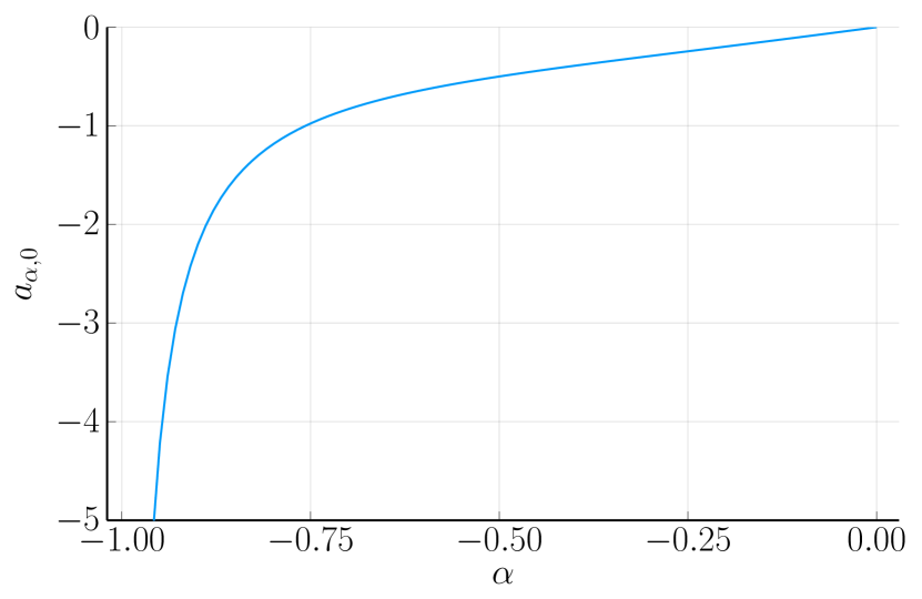
(a)

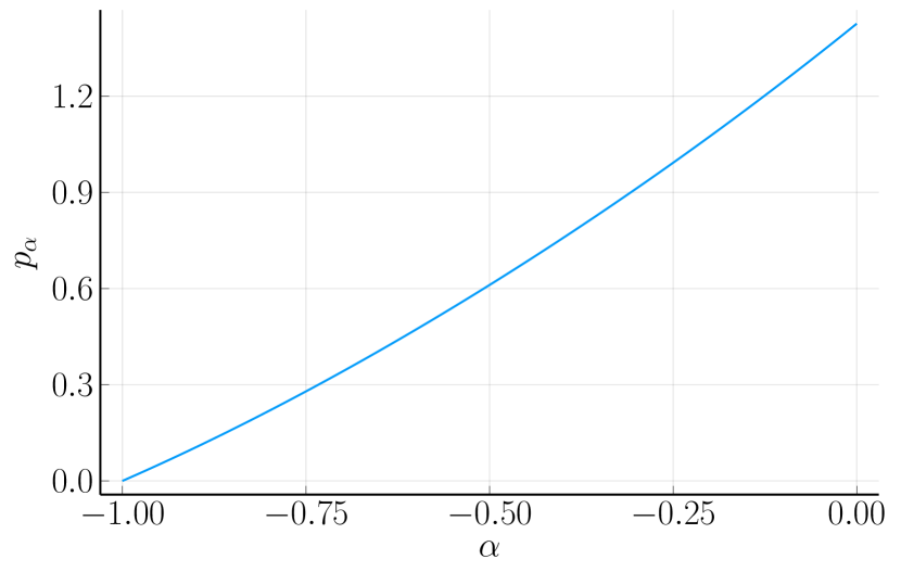
(b)

Figure 1: Values of $a_{\alpha,0}$, defined by Equation (13), and $p_{\alpha}$, defined by Equation (17), as functions of $\alpha$.

The expansion in Lemma 4.3 also tells us how to choose $\{a_{\alpha,j}\}_{1\leq j\leq N_{\alpha,0}}$: identify the $N_{\alpha,0}$ leading coefficients in the expansion, ignoring $|x|^{-2\alpha}$ and $|x|^{-2\alpha+p_{\alpha}}$ whose coefficients are zero from the choice of $a_{\alpha,0}$ and $p_{\alpha}$, and take $\{a_{\alpha,j}\}_{1\leq j\leq N_{\alpha,0}}$ to make them zero. There are three potential issues with this approach for choosing $\{a_{\alpha,j}\}_{1\leq j\leq N_{\alpha,0}}$

1. The coefficients in the expansion might also depend on $b_{\alpha,n}$ which we have yet to determine;

2. It is not clear if we indeed can pick $a_{\alpha,j}$ to make these coefficients zero;

3. Even if we can pick $a_{\alpha,j}$ to make the coefficients zero it is not clear how we would find these values.

The first point is handled by simply ignoring the values of $b_{\alpha,n}$ at this stage, taking them as zero. This means that some of the coefficients in the expansion might not be zero in the end, once the values for $b_{\alpha,n}$ are taken into account. This however turns out to not be an issue, which is related to how to handle the other two points. We summarize it in the following remark

Remark 4.4.

Recall that $u_{\alpha}$ is only an approximate solution to the equation. In the end the only important part is that the defect is sufficiently small. This means that we don’t need to take exact values for $p_{\alpha}$, $\{a_{\alpha,j}\}_{1\leq j\leq N_{\alpha,0}}$ or $\{b_{\alpha,n}\}_{1\leq n\leq N_{\alpha,1}}$. We are free to use any means, in particular non-rigorous numerical methods, for finding values which gives us a small defect. That the defect indeed is small is then later rigorously verified.

Note that this does not apply to the parameter $a_{\alpha,0}$. For the defect to be bounded near $x=0$ we need the leading coefficient in the expansion to be exactly zero, it is therefore not enough to use a numerical approximation of $a_{\alpha,0}$.

I light of this remark, points 2 and 3 above can be dealt with by setting up the problem as a non-linear system of equations and finding a solution using non-rigorous numerical methods. The numerical procedure might or might not converge and the solution it gives might or might not correspond to a true solution, but since we only need approximate value this doesn’t matter. That the solutions we get are good enough will be verified when bounding the defect. Similarly, we don’t need to take $p_{\alpha}$ to be an exact solution of (17), a numerical approximation of the solution suffices.

Once $p_{\alpha}$ and $\{a_{\alpha,j}\}_{1\leq j\leq N_{\alpha,0}}$ have been picked in the above way, to make the asymptotic defect small, we wish to find $\{b_{\alpha,n}\}_{1\leq n\leq N_{\alpha,1}}$ to make the defect small globally. This is done by taking $N_{\alpha,1}$ equally spaced points $\{x_{n}\}_{1\leq n\leq N_{\alpha,1}}$ on the interval $(0,\pi)$ and numerically solving the non-linear system

$$\mathcal{H}^{\alpha}[u_{\alpha}](x_{n})+\frac{1}{2}u_{\alpha}(x_{n})^{2}=0\quad\text{ for }1\leq n\leq N_{\alpha,1}.$$

So far we have not said anything about the values for $N_{\alpha,0}$ and $N_{\alpha,1}$. These are tuning parameters, higher values will typically lead to a smaller defect but also to a higher computational cost. For $N_{\alpha,0}$ this is only true up to some point where the system for determining the coefficients starts to become ill-conditioned. The values are chosen to make sure that the inequality in Proposition 2.2 holds and depends on $\alpha$. Some more details are given in Section 12.2.

4.2 Construction of $u_{\alpha}$ for $I_{1}$

The approximation in the previous section encounters several issues as $\alpha$ moves close to $-1$. To begin with $a_{\alpha,0}$ diverges towards negative infinity, as can be seen in Figure 1(a). Furthermore $p_{\alpha}$ tends towards zero, as can be seen in Figure 1(b), which means that the parameters for all the Clausen functions converge towards the same value.

We can get an idea for how to handle these issues by numerically studying the behavior of

$$\sum_{j=0}^{N_{\alpha,0}}a_{\alpha,j}\tilde{C}_{1-\alpha+jp_{\alpha}}(x),$$ (18)

as $\alpha$ goes to $-1$. The first important observation is that as $\alpha\to-1$ the parameter $a_{\alpha,1}$ goes to infinity in such a way that $a_{\alpha,0}+a_{\alpha,1}$ remains bounded, while $\{a_{\alpha,j}\}_{2\leq j\leq N_{\alpha,0}}$ remains individually bounded. The second important observation is that as $\alpha\to-1$ the parameter $p_{\alpha}$ behaves like $1+\alpha+(1+\alpha)^{2}/2+\mathcal{O}((1+\alpha)^{3})$. This hints at a solution to the problem that $a_{\alpha,0}\tilde{C}_{1-\alpha}(x)$ doesn’t converge: by taking $a_{\alpha,1}=-a_{\alpha,0}$ and $p_{\alpha}=1+\alpha+(1+\alpha)^{2}/2$ the first two terms in the above sum become

$$a_{\alpha,0}(\tilde{C}_{1-\alpha}(x)-\tilde{C}_{2+(1+\alpha)^{2}/2}(x)).$$

For which we have the following lemma.

Lemma 4.5.

The function

$$a_{\alpha,0}(\tilde{C}_{1-\alpha}(x)-\tilde{C}_{2+(1+\alpha)^{2}/2}(x)),$$

with $a_{\alpha,0}$ as in (13), converges to $\frac{2}{\pi^{2}}\tilde{C}_{2}^{(1)}(x)$ pointwise in $x$ as $\alpha\to-1$. Moreover, for $\alpha\in\left(-1,-\frac{3}{4}\right)$ it satisfies the inequality

$$a_{\alpha,0}(\tilde{C}_{1-\alpha}(x)-\tilde{C}_{2+(1+\alpha)^{2}/2}(x))\geq\frac{2}{\pi^{2}}\tilde{C}_{2}^{(1)}(x).$$

Proof.

We have

$$a_{\alpha,0}(\tilde{C}_{1-\alpha}(x)-\tilde{C}_{2+(1+\alpha)^{2}/2}(x))=-(1+\alpha)a_{\alpha,0}\cdot\frac{\tilde{C}_{2+(1+\alpha)^{2}/2}(x)-\tilde{C}_{1-\alpha}(x)}{1+\alpha}.$$

Taking the limit as $\alpha\to-1$ for the first factor we get $\lim_{\alpha\to-1}-(1+\alpha)a_{\alpha,0}=\frac{2}{\pi^{2}}.$ The second factor converges to the derivative $\tilde{C}_{1-\alpha}^{(1)}(x)$. This gives us the pointwise convergence.

To prove the inequality it is enough to prove that the left-hand side is increasing in $\alpha$. For that it is enough to prove that both factors are positive and increasing in $\alpha$.

The proof that $-(1+\alpha)a_{\alpha,0}$ is positive and increasing in $\alpha$ is computer-assisted. It is done by rigorously computing a lower bound of the value and the derivative for $-1<\alpha<-\frac{3}{4}$ and asserting that these lower bounds are positive.

For the Clausen-factor we let $h=1+\alpha$ and expand the Clausen functions at $s=2$, giving us

$$\tilde{C}_{1-\alpha}(x) =\sum_{n=0}^{\infty}\frac{\tilde{C}_{2}^{(n)}(x)}{n!}(-h)^{n},$$

$$\tilde{C}_{1+(1+\alpha)^{2}/2}(x) =\sum_{n=0}^{\infty}\frac{\tilde{C}_{2}^{(n)}(x)}{n!}\left(\frac{h^{2}}{2}\right)^{n}.$$

From which we get

$$\frac{\tilde{C}_{2+(1+\alpha)^{2}/2}(x)-\tilde{C}_{1-\alpha}(x)}{1+\alpha}=\sum_{n=1}^{\infty}\frac{\tilde{C}_{2}^{(n)}(x)}{n!}h^{n-1}\left(\frac{h^{n}}{2^{n}}+(-1)^{n-1}\right).$$ (19)

For $-1<\alpha<0$ we have $\left|\frac{h^{n}}{2^{n}}\right|<1$ and the sign of the factor $\frac{h}{2^{n}}+(-1)^{n-1}$ is therefore the same as for $(-1)^{n-1}$. Furthermore, we have

$$\tilde{C}_{2}^{(n)}(x)=(-1)^{n}\sum_{k=1}^{\infty}\frac{\cos(kx)-1}{k^{2}}\log k$$

and since $\cos(kx)-1\leq 0$ this has the same sign as $(-1)^{n-1}$. It follows that all the terms in (19) are positive, hence the sum is positive and increasing in $\alpha$ for $-1<\alpha<0$. ∎

If we subtract $a_{\alpha,0}(\tilde{C}_{1-\alpha}(x)-\tilde{C}_{2+(1+\alpha)^{2}/2}(x))$ from (18) the remaining part of

$$(a_{\alpha,0}+a_{\alpha,1})\tilde{C}_{1-\alpha+jp_{\alpha}}(x)+\sum_{j=2}^{N_{\alpha,0}}a_{\alpha,j}\tilde{C}_{1-\alpha+jp_{\alpha}}(x),$$

Numerically we can see that this converges to a bounded function as $\alpha$ goes towards $-1$. Since we only need an approximation of the limit we can simply fix some $\alpha>-1$ and use the values for this $\alpha$.

More precisely we construct the approximation for $I_{1}$ in the following way. First fix $\hat{\alpha}$ close to $-1$ but such that $\alpha<\hat{\alpha}$ for all $\alpha\in I_{1}$. Then compute $\{a_{\hat{\alpha},j}\}_{0\leq j\leq N_{\hat{\alpha},1}}$ and $p_{\hat{\alpha}}$ using the approach in Section 4.1. We then take

$$u_{\alpha}(x)=a_{\alpha,0}(\tilde{C}_{1-\alpha}(x)-\tilde{C}_{2+(1+\alpha)^{2}/2}(x))+(a_{\hat{\alpha},0}+a_{\hat{\alpha},1})\tilde{C}_{1-\hat{\alpha}+p_{\hat{\alpha}}}(x)\\ +\sum_{j=2}^{N_{\hat{\alpha},0}}a_{\hat{\alpha},j}\tilde{C}_{1-\hat{\alpha}+jp_{\hat{\alpha}}}(x)+\sum_{n=1}^{N_{-1,1}}b_{-1,n}(\cos(nx)-1)$$ (20)

The parameters $\{b_{-1,n}\}_{1\leq n\leq N_{-1,1}}$ are determined by considering the defect at the limit $\alpha\to-1$, where we from Lemma 4.5 have

$$u_{-1}(x)=\frac{2}{\pi^{2}}\tilde{C}_{2}^{(1)}(x)+(a_{\hat{\alpha},0}+a_{\hat{\alpha},1})\tilde{C}_{1-\hat{\alpha}+p_{\hat{\alpha}}}(x)+\sum_{j=2}^{N_{\hat{\alpha},0}}a_{\hat{\alpha},j}\tilde{C}_{1-\hat{\alpha}+jp_{\hat{\alpha}}}(x)+\sum_{n=1}^{N_{-1,1}}b_{-1,n}(\cos(nx)-1).$$ (21)

In the same way as in Section 4.1 we take $\{b_{-1,n}\}_{1\leq n\leq N_{-1,1}}$ so that the defect is minimized on $N_{-1,1}$ equally spaced points on the interval $(0,\pi)$. Note that by Lemma 4.5 $u_{-1}(x)$ gives a lower bound of $u_{\alpha}(x)$.

With this approximation we get

$$\mathcal{H}^{\alpha}[u_{\alpha}](x)=-a_{\alpha,0}(\tilde{C}_{1-2\alpha}(x)-\tilde{C}_{2-\alpha+(1+\alpha)^{2}/2}(x))+(a_{\hat{\alpha},0}+a_{\hat{\alpha},1})\tilde{C}_{1-\alpha-\hat{\alpha}+p_{\hat{\alpha}}}(x)\\ -\sum_{j=2}^{N_{\hat{\alpha},0}}a_{\hat{\alpha},j}\tilde{C}_{1-\alpha-\hat{\alpha}+jp_{\hat{\alpha}}}(x)-\sum_{n=1}^{N_{-1,1}}b_{-1,n}n^{-\alpha}(\cos(nx)-1).$$ (22)

Note that since $a_{\alpha,0}\to-\infty$ as $\alpha\to-1$ we cannot compute a finite enclosure of $a_{\alpha,0}$ valid for an interval of the form $(-1,-1+\delta)$. When computing enclosures we therefore have to treat

$$a_{\alpha,0}(\tilde{C}_{1-\alpha}(x)-\tilde{C}_{2+(1+\alpha)^{2}/2}(x))\quad\text{and}\quad a_{\alpha,0}(\tilde{C}_{1-2\alpha}(x)-\tilde{C}_{2-\alpha+(1+\alpha)^{2}/2}(x))$$

as one part, and explicitly handle the removable singularity.

The asymptotic behavior are given in the following lemma, again we omit the proof since it follows directly from the expansions of the Clausen functions.

Lemma 4.6.

The approximation for $\alpha\in I_{1}$, with $u_{\alpha}$ given by (20) and $\mathcal{H}^{\alpha}[u_{\alpha}]$ given by (22) has the asymptotic expansions

$$u_{\alpha}(x)= a_{\alpha,0}\left(\Gamma(\alpha)\cos\left(\frac{\pi}{2}\alpha\right)-\Gamma(-1-(1+\alpha)^{2}/2)\cos\left(\frac{\pi}{2}(1+(1+\alpha)^{2}/2)\right)|x|^{1+\alpha+(1+\alpha)^{2}/2}\right)|x|^{-\alpha}$$

$$+a_{\alpha,0}\sum_{m=1}^{\infty}\frac{(-1)^{m}}{(2m)!}\left(\zeta(1-\alpha-2m)-\zeta(2+(1+\alpha)^{2}/2-2m)\right)x^{2m}$$

$$+\sum_{j=1}^{N_{\hat{\alpha},0}}\hat{a}_{\alpha,j}^{0}|x|^{-\hat{\alpha}+jp_{\hat{\alpha}}}+\sum_{m=1}^{\infty}\frac{(-1)^{m}}{(2m)!}\left(\sum_{j=1}^{N_{\hat{\alpha},0}}a_{\hat{\alpha},j}\zeta(1-\hat{\alpha}+jp_{\hat{\alpha}}-2m)+\sum_{m=1}^{N_{-1,1}}b_{\hat{\alpha},j}n^{2m}\right)x^{2m}$$

and

$$\mathcal{H}^{\alpha}u_{\alpha}(x)= -a_{\alpha,0}\left(\Gamma(2\alpha)\cos\left(\pi\alpha\right)-\Gamma(-1+\alpha-(1+\alpha)^{2}/2)\cos\left(\frac{\pi}{2}(1-\alpha+(1+\alpha)^{2}/2)\right)|x|^{1+\alpha+(1+\alpha)^{2}/2}\right)|x|^{-2\alpha}$$

$$-a_{\alpha,0}\sum_{m=1}^{\infty}\frac{(-1)^{m}}{(2m)!}\left(\zeta(1-2\alpha-2m)-\zeta(2-\alpha+(1+\alpha)^{2}/2-2m)\right)x^{2m}$$

$$-\sum_{j=1}^{N_{\hat{\alpha},0}}\hat{A}_{\alpha,j}^{0}|x|^{-\alpha-\hat{\alpha}+jp_{\hat{\alpha}}}-\sum_{m=1}^{\infty}\frac{(-1)^{m}}{(2m)!}\left(\sum_{j=1}^{N_{\hat{\alpha},0}}a_{\hat{\alpha},j}\zeta(1-\alpha-\hat{\alpha}+jp_{\hat{\alpha}}-2m)+\sum_{m=1}^{N_{-1,1}}b_{\hat{\alpha},j}n^{2m+\alpha}\right)x^{2m},$$

where

$$\hat{a}_{\alpha,j}^{0} =\Gamma(\hat{\alpha}-jp_{\hat{\alpha}})\cos\left(\frac{\pi}{2}(\hat{\alpha}-jp_{\hat{\alpha}})\right)a_{\hat{\alpha},j};$$

$$\hat{A}_{j}^{0} =\Gamma(\alpha+\hat{\alpha}-jp_{\hat{\alpha}})\cos\left(\frac{\pi}{2}(\alpha+\hat{\alpha}-jp_{\hat{\alpha}})\right)a_{\hat{\alpha},j}.$$

There are a couple of things that make these expansions tricky to handle. To begin with the terms $a_{\alpha,0}(\zeta(1-\alpha-2m)-\zeta(2+(1+\alpha)^{2}/2-2m))$ in $u_{\alpha}$ have removable singularities at $\alpha=-1$, this is handled using the approach described in Appendix A. For $\mathcal{H}^{\alpha}[u_{\alpha}]$ the exponent for the term

$$-a_{\alpha,0}\left(\Gamma(2\alpha)\cos\left(\pi\alpha\right)-\Gamma(-1+\alpha-(1+\alpha)^{2}/2)\cos\left(\frac{\pi}{2}(1-\alpha+(1+\alpha)^{2}/2)\right)|x|^{1+\alpha+(1+\alpha)^{2}/2}\right)|x|^{-2\alpha}$$

approaches $2$ and its interaction with the $x^{2}$ term

$$-\frac{1}{2}a_{\alpha,0}\left(\zeta(1-2\alpha-2)-\zeta(2-\alpha+(1+\alpha)^{2}/2-2)\right)x^{2}$$

needs special care. A similar thing happens for $\hat{A}_{\alpha,j}^{0}|x|^{-\alpha-\hat{\alpha}+jp_{\hat{\alpha}}}$ and the corresponding $x^{2}$ terms. How this is handled is discussed in detail in Section 10.2 and Appendix E. Bounding the tails of the sum

$$\sum_{m=1}^{\infty}\frac{(-1)^{m}}{(2m)!}a_{\alpha,0}\left(\zeta(1-\alpha-2m)-\zeta(2+(1+\alpha)^{2}/2-2m)\right)x^{2m}$$

and the corresponding one for $\mathcal{H}^{\alpha}[u_{\alpha}]$ requires a bit extra work, this is done in Lemma C.7 and C.8.

For the precise values of $\hat{\alpha}$, $N_{\hat{\alpha},0}$ and $N_{-1,1}$ see Section 12.1.

4.3 Construction of $u_{\alpha}$ for $I_{3}$

Using the approximation from Section 4.1 and letting $\alpha$ tend to $0$ it turns out that we need fewer and fewer terms to get a small defect. For $\alpha$ close to $0$ (around $-1/6$ or closer) it is enough to take $N_{\alpha,0}=2$ and $N_{\alpha,1}=0$, giving us the approximation

$$u_{\alpha}(x)=\sum_{j=0}^{2}a_{\alpha,j}\tilde{C}_{1-\alpha+jp_{\alpha}}(x)$$ (23)

and

$$\mathcal{H}^{\alpha}[u_{\alpha}](x)=-\sum_{j=0}^{2}a_{\alpha,j}\tilde{C}_{1-2\alpha+jp_{\alpha}}(x).$$ (24)

With this approximation the defect tends to zero as $\alpha\to 0$, which is good. However, in Section 11.2.3 we will see that the value of $D_{\alpha}$ in Proposition 2.2 tends to $1$, meaning that $(1-D_{\alpha})^{2}/4n_{\alpha}$ also tends to zero. This means that we can never compute an enclosure for $D_{\alpha}$ and $\delta_{\alpha}$ on any interval $(-\delta_{2},0)$ such that the inequality in Proposition 2.2 holds. Instead, we compute expansions in $\alpha$ at $\alpha=0$ of both $D_{\alpha}$ and $\delta_{\alpha}$, using these expansions we can then prove that the inequality holds on the interval $I_{3}$.

In this case it is not enough to use numerical approximations of $a_{\alpha,1}$, $a_{\alpha,2}$ and $p_{\alpha}$, we need to take into account their dependence on $\alpha$. For $p_{\alpha}$ we use the defining equation (17). As $\alpha\to 0$ we have $p_{\alpha}\to 1.426\dots$, this gives us that the four leading terms (in $x$) in the expansion from Lemma 4.3 are given by, ordered by their exponents,

$$\left(\frac{1}{2}(a_{\alpha,0}^{0})^{2}-A_{\alpha,0}^{0}\right)|x|^{-2\alpha},$$

$$\left(a_{\alpha,0}^{0}a_{\alpha,1}^{0}-A_{\alpha,1}^{0}\right)|x|^{-2\alpha+p_{\alpha}},$$

$$\frac{1}{2}\left(\sum_{j=0}^{2}a_{\alpha,j}\zeta(-1-2\alpha+jp_{\alpha})\right)x^{2},$$

$$-\frac{1}{2}a_{\alpha,0}^{0}\left(\sum_{j=0}^{2}a_{\alpha,j}\zeta(-1-\alpha+jp_{\alpha})\right)x^{2-\alpha}.$$

The choice of $a_{\alpha,0}$ makes the first term zero and the choice of $p_{\alpha}$ makes the second term zero. We then want to take $a_{\alpha,1}$ and $a_{\alpha,2}$ to make the third and fourth term zero. Solving for $a_{\alpha,1}$ and $a_{\alpha,2}$ we get the linear system

$$\begin{cases}a_{\alpha,1}\zeta(-1-2\alpha+p_{\alpha})+a_{\alpha,2}\zeta(-1-2\alpha+2p_{\alpha})&=-a_{\alpha,0}\zeta(-1-2\alpha)\\ a_{\alpha,1}\zeta(-1-\alpha+p_{\alpha})+a_{\alpha,2}\zeta(-1-\alpha+2p_{\alpha})&=-a_{\alpha,0}\zeta(-1-\alpha)\end{cases},$$

with the solution

$$\begin{cases}a_{\alpha,1}&=a_{\alpha,0}\frac{\zeta(-1-\alpha)\zeta(-1-2\alpha+2p_{\alpha})-\zeta(-1-2\alpha)\zeta(-1-\alpha+2p_{\alpha})}{\zeta(-1-2\alpha+p_{\alpha})\zeta(-1-\alpha+2p_{\alpha})-\zeta(-1-2\alpha+2p_{\alpha})\zeta(-1-\alpha+p_{\alpha})}\\ a_{\alpha,2}&=-a_{\alpha,0}\frac{\zeta(-1-\alpha)\zeta(-1-2\alpha+p_{\alpha})-\zeta(-1-2\alpha)\zeta(-1-\alpha+p_{\alpha})}{\zeta(-1-2\alpha+p_{\alpha})\zeta(-1-\alpha+2p_{\alpha})-\zeta(-1-2\alpha+2p_{\alpha})\zeta(-1-\alpha+p_{\alpha})}\end{cases}.$$ (25)

The following lemma gives us information about the asymptotic behavior of $a_{\alpha,j}$.

Lemma 4.7.

The expansion of $a_{\alpha,0}$ at $\alpha=0$ is given by

$$a_{\alpha,0}=\alpha+\mathcal{O}(\alpha^{3}).$$

For $a_{\alpha,1}$ and $a_{\alpha,2}$ it is given by

$$a_{\alpha,j}=a_{\alpha,j,1}\alpha+\mathcal{O}(\alpha^{2})$$

with

$$a_{\alpha,1,1}=\lim_{\alpha\to 0}\frac{\zeta(-1-\alpha)\zeta(-1-2\alpha+2p_{\alpha})-\zeta(-1-2\alpha)\zeta(-1-\alpha+2p_{\alpha})}{\zeta(-1-2\alpha+p_{\alpha})\zeta(-1-\alpha+2p_{\alpha})-\zeta(-1-2\alpha+2p_{\alpha})\zeta(-1-\alpha+p_{\alpha})}$$

and

$$a_{\alpha,2,1}=\lim_{\alpha\to 0}\frac{\zeta(-1-2\alpha)\zeta(-1-\alpha+p_{\alpha})-\zeta(-1-\alpha)\zeta(-1-\alpha+2p_{\alpha})}{\zeta(-1-2\alpha+p_{\alpha})\zeta(-1-\alpha+2p_{\alpha})-\zeta(-1-2\alpha+2p_{\alpha})\zeta(-1-\alpha+p_{\alpha})}.$$

Proof.

The expansion for $a_{\alpha,0}$ follows from Equation (13) by using that $\Gamma(\alpha)=\alpha^{-1}+\gamma+\mathcal{O}(\alpha)$, giving us

$$a_{\alpha,0}=\frac{2\left((2\alpha)^{-1}+\gamma+\mathcal{O}(\alpha)\right)(1+\mathcal{O}(\alpha^{2}))}{(\alpha^{-1}+\gamma+\mathcal{O}(\alpha))^{2}(1+\mathcal{O}(\alpha^{2}))}=\frac{\alpha^{-1}+2\gamma+\mathcal{O}(\alpha)}{\alpha^{-2}+2\gamma\alpha^{-1}+\mathcal{O}(1)}=\alpha\frac{1+2\gamma\alpha+\mathcal{O}(\alpha^{2})}{1+2\gamma\alpha+\mathcal{O}(\alpha^{2})}=\alpha+\mathcal{O}(\alpha^{3}).$$

The expansions for $a_{\alpha,1}$ and $a_{\alpha,2}$ follows directly from Equation (25). ∎

Using this we can get information about the asymptotic behavior of $u_{\alpha}$ and $\mathcal{H}^{\alpha}[u_{\alpha}]$.

Lemma 4.8.

For $x\in(0,\pi]$ we have the following expansions at $\alpha=0$:

$$u_{\alpha}(x) =1+b(x)\alpha+\mathcal{O}(\alpha^{2}),$$

$$\mathcal{H}^{\alpha}[u_{\alpha}](x) =-\frac{1}{2}-b(x)\alpha+\mathcal{O}(\alpha^{2}),$$

with

$$b(x)=C_{1}(x)-\gamma+a_{\alpha,1,1}\tilde{C}_{1+p_{0}}(x)+a_{\alpha,2,1}\tilde{C}_{1+2p_{0}}(x).$$

Proof.

For $j\geq 1$ the Clausen functions are all finite at $\alpha=0$ and from Lemma 4.7 we therefore get

$$a_{\alpha,1}\tilde{C}_{1-\alpha+p_{\alpha}}(x) =a_{\alpha,1,1}\tilde{C}_{1+p_{0}}(x)\alpha+\mathcal{O}(\alpha^{2}),$$

$$a_{\alpha,2}\tilde{C}_{1-\alpha+2p_{\alpha}}(x) =a_{\alpha,2,1}\tilde{C}_{1+2p_{0}}(x)\alpha+\mathcal{O}(\alpha^{2}),$$

$$a_{\alpha,1}\tilde{C}_{1-2\alpha+p_{\alpha}}(x) =a_{\alpha,1,1}\tilde{C}_{1+p_{0}}(x)\alpha+\mathcal{O}(\alpha^{2}),$$

$$a_{\alpha,2}\tilde{C}_{1-2\alpha+p_{\alpha}}(x) =a_{\alpha,2,1}\tilde{C}_{1+2p_{0}}(x)\alpha+\mathcal{O}(\alpha^{2}).$$

For $j=0$ the function $\tilde{C}_{1-\alpha}(x)$ has a singularity at $\alpha=0$. More precisely

$$\tilde{C}_{1-\alpha}(x)=C_{1-\alpha}(x)-\zeta(1-\alpha),$$

where for $0<x<2\pi$ the factor $C_{1-\alpha}(x)$ is finite, but $\zeta(1-\alpha)$ has a singularity at $\alpha=0$, similarly for $\tilde{C}_{1-2\alpha}(x)$. After multiplying with $a_{\alpha,0}$ the singularity is removable. To begin with we have

$$a_{\alpha,0}C_{1-\alpha}(x)=C_{1}(x)\alpha+\mathcal{O}(\alpha^{2}).$$

Using the Laurent series of the zeta function we have

$$\zeta(1-\alpha)=-\alpha^{-1}+\sum_{n=0}^{\infty}\frac{1}{n!}\gamma_{n}\alpha^{n}=-\alpha^{-1}+\gamma+\mathcal{O}(\alpha),$$

where $\gamma_{n}$ is the Stieltjes constant and $\gamma=\gamma_{0}$ is Euler’s constant, from which we get

$$a_{\alpha,0}\zeta(1-\alpha)=(\alpha+\mathcal{O}(\alpha^{3}))(-\alpha^{-1}+\gamma+\mathcal{O}(\alpha))=-1+\gamma\alpha+\mathcal{O}(\alpha^{2}).$$

Giving us

$$a_{\alpha,0}\tilde{C}_{1-\alpha}(x)=1+(C_{1}(x)-\gamma)\alpha+\mathcal{O}(\alpha^{2}).$$

In the same way we get

$$a_{\alpha,0}\tilde{C}_{1-2\alpha}(x)=\frac{1}{2}+(C_{1}(x)-\gamma)\alpha+\mathcal{O}(\alpha^{2}).$$

Combining all the above gives us

$$u_{\alpha}(x)=1+(C_{1}(x)-\gamma+\tilde{C}_{1+p_{0}}(x)+\tilde{C}_{1+2p_{0}}(x))\alpha+\mathcal{O}(\alpha^{2})$$

and

$$\mathcal{H}^{\alpha}[u_{\alpha}](x)=-\frac{1}{2}-(C_{1}(x)-\gamma+\tilde{C}_{1+p_{0}}(x)+\tilde{C}_{1+2p_{0}}(x))\alpha+\mathcal{O}(\alpha^{2}),$$

from which the result follows. ∎

4.4 Hybrid cases

While it is technically possible to use the construction from Section 4.1 to handle the entire interval $I_{2}$ it is not computationally feasible. As $\alpha$ gets close to either $-1$ or $0$ the bounds that needs to be computed becomes harder and harder to handle.

For $\alpha$ near $0$ it is mainly bounding $\delta_{\alpha}$ that becomes hard to deal with. It goes to zero as $\alpha\to 0$, which means that absolute errors in the bound that are negligible when $\delta_{\alpha}$ is larger quickly grow to become very large relative errors.

Near $\alpha=-1$ it is mainly the behavior of $F_{\alpha}(x)$ and $\mathcal{T}_{\alpha}(x)$ (from Equation (31)) around $x=0$ that become problematic. This is related to the powers for the terms $\nu_{\alpha}|x|^{-\alpha}$ and $\mathcal{O}(|x|^{p})$ in Theorem 1.1 getting closer and closer to each other, giving us less space to work with. Another issue is, as mentioned in Section 4.2, that the two Clausen functions $a_{\alpha,0}\tilde{C}_{1-\alpha}$ and $a_{\alpha,1}\tilde{C}_{1-\alpha+p_{\alpha}}$ grow quickly in opposite directions as $\alpha$ gets closer to $-1$ and as a result there are large cancellations to handle.

For $\alpha$ near $0$ we use the approximation from Equation (23), but instead of using expansions centered at $\alpha=0$ we use expansions centered at $\alpha$ (or the midpoint, when computing with intervals). Compared to the case $\alpha=0$ there are no removable singularities to handle, which makes the process simpler.

For $\alpha$ near $-1$ we use the ideas from Section 4.2 for handling $\alpha\in I_{1}$. Instead of using

$$u_{\alpha}(x)=\sum_{j=0}^{N_{\alpha,0}}a_{\alpha,j}\tilde{C}_{1-\alpha+jp_{\alpha}}(x)+\sum_{n=1}^{N_{\alpha,1}}b_{\alpha,n}(\cos(nx)-1),$$

from Equation (12) we modify it in the same spirit as Equation (20). More precisely we use

$$u_{\alpha}(x)=a_{\alpha,0}(\tilde{C}_{1-\alpha}(x)-\tilde{C}_{1-\alpha+p_{\alpha}}(x))+\hat{a}_{\alpha,1}\tilde{C}_{1-\alpha+p_{\alpha}}(x)+\sum_{j=2}^{N_{\alpha,0}}a_{\alpha,j}\tilde{C}_{1-\alpha+jp_{\alpha}}(x)+\sum_{n=1}^{N_{\alpha,1}}b_{\alpha,n}(\cos(nx)-1).$$

If we take $\hat{a}_{\alpha,1}=a_{\alpha,0}+a_{\alpha,1}$ this is equivalent to Equation (20) The benefit with this approach is that we don’t have to use an enclosure of $a_{\alpha,0}$ in $\hat{a}_{\alpha,1}$, but can take a numerical approximation instead.

In both cases we make adjustments to how the bounds are computed, the details are given in the relevant sections.

5 Choice of $w_{\alpha}$

In the above section we discussed how to construct the approximation $u_{\alpha}$ for the ansatz (7). We here discuss the choice of the weight $w_{\alpha}$ in the ansatz. To get the statement in Theorem 1.1 we need $w_{\alpha}(x)=\mathcal{O}(|x|^{p})$ for some $p$ satisfying $-\alpha<p\leq 1$. The natural choice is $w_{\alpha}(x)=|x|$, however this turns out to not work for all values of $\alpha$.

The main obstruction when choosing $w_{\alpha}$ is its effect on the value of $D_{\alpha}$. For Proposition 2.2 to apply we require that $D_{\alpha}<1$, if we take $w_{\alpha}(x)=|x|$ this is not always the case. Using the procedure described in Section 11, in particular lemma 11.7, we can compute a lower bound of $D_{\alpha}$ by computing $\mathcal{T}_{\alpha}(0)$, introduced in (31) and (30). A plot of $\mathcal{T}_{\alpha}(0)$ as a function of $\alpha$, using $w_{\alpha}(x)=|x|$, is given in Figure 2. From this plot we can see that with the weight $w_{\alpha}(x)=|x|$ we have $D_{\alpha}>1$ for $\alpha$ between $-1$ and some value slightly smaller than $-0.5$, in which case Proposition 2.2 won’t apply.

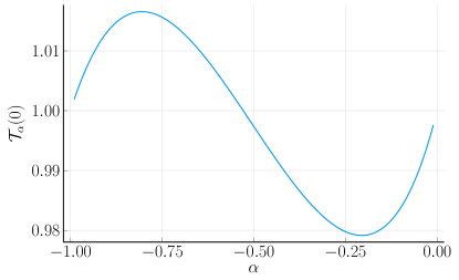
Figure 2: Value of $\mathcal{T}_{\alpha}(0)$, defined by (31), as a function of $\alpha$ using the weight $w_{\alpha}(x)=|x|$. This gives a lower bound of $D_{\alpha}$ and since we need $D_{\alpha}<1$ it means that this choice of weight does not work for all values of $\alpha$.

By taking $w_{\alpha}(x)=|x|^{p}$ with $-\alpha<p<1$ the value of $D_{\alpha}$ can be made smaller than $1$, so that Proposition 2.2 applies. The precise value of $p$ to use depends on $\alpha$ and is made more precise in Section 12.2.

The limits $\alpha\to-1$ and $\alpha\to 0$ both require extra attention. For $\alpha\to 0$ with the weight $w_{\alpha}(x)=|x|$ the value of $D_{\alpha}$ tends to $1$. However, in this case $\delta_{\alpha}$ tends to $0$ and by controlling the rate of convergence of $D_{\alpha}$ and $\delta_{\alpha}$ it is still possible to apply Proposition 2.2, see Section 12.3 for more details.

For $\alpha\to-1$ the situation is more complicated. It is not possible to use the weight $w_{\alpha}(x)=|x|$ because $D_{\alpha}$ would be strictly greater than $1$ close to $\alpha=-1$. It is also not possible to use the weight $w_{\alpha}(x)=|x|^{p}$ with $p$ satisfying $-\alpha<p<1$ since in the limit we would have need to have $p\to 1$, and again we find that $D_{\alpha}$ is greater than $1$. A natural choice would be to add a log-factor, $w_{\alpha}(x)=|x|\log(1+1/|x|)$. Lengthy calculations however shows that this would not work either. Instead, we have to take $w_{\alpha}(x)$ to behave like $|x|^{p}\log(1+1/|x|)$ with $p<1$ and $p\to 1$ as $\alpha\to-1$. More precisely we take $w_{\alpha}(x)=|x|^{(1-\alpha)/2}\log(2e+1/|x|)$, the constant $2e$ does not change the asymptotic behavior close to $x=0$ but does change the non-asymptotic behavior in a way that turns out to make it slightly easier to satisfy the required inequality in Proposition 2.2. That we have to take such a complicated weight, compared to just $w_{\alpha}(x)=|x|^{p}$, makes the analysis of $D_{\alpha}$ in Section 11 significantly harder.

For the hybrid cases we mimic what happens at the endpoints. Summarizing we have the following choice for $w_{\alpha}$:

• For $\alpha\in I_{1}$ we take $w_{\alpha}(x)=|x|^{(1-\alpha)/2}\log(2e+1/|x|)$.

• For $\alpha\in I_{2}$ we have three cases

  • Near $\alpha=-1$ we take $w_{\alpha}(x)=|x|^{p}\log(2e+1/|x|)$ with $-\alpha<p<1$.

  • Near $\alpha=0$ we take $w_{\alpha}(x)=|x|$

  • In between we take $w_{\alpha}(x)=|x|^{p}$ with $-\alpha<p<1$.

  The precise choice of $p$ as a function of $\alpha$ is given in Section 12.2.

• For $\alpha\in I_{3}$ we take $w_{\alpha}(x)=|x|$.

6 Proof strategy

The main part of the proof of Theorem 1.1 is the computation of the bounds of $n_{\alpha}$, $\delta_{\alpha}$ and $D_{\alpha}$ required to apply Proposition 2.2. Explicit bounds of these values are given in Section 12. In this section we describe the general procedure for computing these bounds. The details for the different cases are given in Sections 7 to 11.

The values we want to bound are given by

$$n_{\alpha}=\sup_{x\in[0,\pi]}|N_{\alpha}(x)|,\quad\delta_{\alpha}=\sup_{x\in[0,\pi]}|F_{\alpha}(x)|,\quad D_{\alpha}=\sup_{x\in[0,\pi]}|\mathcal{T}_{\alpha}(x)|.$$

With $N_{\alpha}$ and $F_{\alpha}$ as in (10) and (9) in Section 2 and $\mathcal{T}_{\alpha}$ as in (31) in Section 11. At $x=0$ the functions all have removable singularities, for small values of $x$ the functions therefore need extra care when evaluating them. For that reason the computation of the supremum is split into two parts, one on the interval $[0,\epsilon]$ and one on the interval $[\epsilon,\pi]$, for some $\epsilon$ depending on $\alpha$ and the function. On the interval $[0,\epsilon]$ we use a method of evaluation which takes into account the removable singularity.

To enclose the supremum on the intervals $[0,\epsilon]$ and $[\epsilon,\pi]$ we make use of methods from interval arithmetic and rigorous numerics. In this section we give a brief description of these methods and also discuss what we require of $N_{\alpha}$, $F_{\alpha}$ and $\mathcal{T}_{\alpha}$ to be able to apply these methods.

6.1 Enclosing the supremum

Consider the general problem of enclosing the maximum of $f$ on some interval $I$ to some predetermined tolerance. Assume that we can evaluate $f$ using interval arithmetic, i.e. given any interval $\textbf{{x}}\subseteq I$ we can compute an interval enclosing the set $f(\textbf{{x}})=\{f(x):x\in\textbf{{x}}\}$. The main idea is to iteratively bisect the interval $I$ into smaller and smaller subintervals. At every iteration we compute an enclosure of $f$ on each subinterval. From these enclosures a lower bound of the maximum can be computed. We then discard all subintervals for which the enclosure is less than the lower bound of the maximum, the maximum cannot be attained there. For the remaining subintervals we check if their enclosure satisfies the required tolerance, in that case we don’t bisect them further. If there are any subintervals left we bisect them and continue with the next iteration. In the end, either when there are no subintervals left to bisect or we have reached some maximum number of iterations (to guarantee that the procedure terminates), we return the maximum of all subintervals that were not discarded. This is guaranteed to give an enclosure of the maximum of $f$ on the interval.

If we are able to compute Taylor expansions of the function $f$ we can improve the performance of this procedure significantly (see e.g. [17, 16] where a similar approach is used). Consider a subinterval $I_{i}$, instead of computing an enclosure of $f(I_{i})$ we compute a Taylor polynomial $P$ at the midpoint and an enclosure $R$ of the remainder term such that $f(x)\in P(x)+R$ for $x\in I_{i}$. We then have

$$\sup_{x\in I_{i}}f(x)\in\sup_{x\in I_{i}}P(x)+R.$$ (26)

To compute $\sup_{x\in I_{i}}P(x)$ we isolate the roots of $P^{\prime}$ on $I_{i}$ and evaluate $P$ on the roots as well as the endpoints of the interval. In practice the computation of $R$ involves computing an enclosure of the Taylor expansion of $f$ on the full interval $I_{i}$. Since this includes the derivative we can as an extra optimization check if the derivative is non-zero, in which case $f$ is monotone, and it is enough to evaluate $f$ on either the left or the right endpoint of $I_{i}$, depending on the sign of the derivative.

The above procedures can easily be adapted to instead compute the minimum of $f$ on the interval, joining them together we can thus compute the extrema on the interval. In some cases we don’t care about computing an enclosure of the maximum, but only to prove that it is bounded by some value. Instead of using a tolerance we then discard any subintervals for which the enclosure of the maximum is less than the bound.

6.2 Evaluation of $N_{\alpha}$, $F_{\alpha}$ and $\mathcal{T}_{\alpha}$ on intervals

To be able to use the above method we need to be able to evaluate $N_{\alpha}$, $F_{\alpha}$ and $\mathcal{T}_{\alpha}$ using interval arithmetic. That is, given some interval $\textbf{{x}}\subseteq[0,\pi]$ we need to be able to compute enclosures of $N_{\alpha}(\textbf{{x}})$, $F_{\alpha}(\textbf{{x}})$ and $\mathcal{T}_{\alpha}(\textbf{{x}})$ respectively.

In Sections 7 to 11 we discuss how to evaluate these functions for (non-interval) $x\in[0,\pi]$. This then needs to be extended to also work for intervals $\textbf{{x}}\subseteq(0,\pi)$. In general this is straight forward and handled directly by just replacing the point $x\in[0,\pi]$ with the interval $\textbf{{x}}\subseteq(0,\pi)$ in the computations, the operations on the interval are then done using Arb [40]. In some cases we can make use of monotonicity properties of the function. For example when computing the root $r_{\alpha,x}$ introduced in Lemma 11.2 for an interval $\textbf{{x}}=[\underline{x},\overline{x}]$ we can use that it is decreasing in $x$, giving us $r_{\alpha,\textbf{{x}}}=[r_{\alpha,\overline{x}},r_{\alpha,\underline{x}}].$.

To cover all values of $\alpha$ in $(-1,0)$ we need to use interval values also for $\alpha$, and not only for $x$. Similar to $x$ this is in general done by just replacing $\alpha\in(-1,0)$ with $\boldsymbol{\alpha}\subseteq(-1,0)$ in the computations.

To be able to use the improved version of the method for enclosing the supremum discussed in Section 6.1 we need to be able to compute Taylor expansions of $N_{\alpha}$, $F_{\alpha}$ and $\mathcal{T}_{\alpha}$. This is possible in many, but not all cases. For $x\in[\epsilon,\pi]$ this is in general straight forward for $N_{\alpha}$ and $F_{\alpha}$, for example the methods in Appendix C.2 can be used for computing Taylor expansions of the involved Clausen functions, but not for $\mathcal{T}_{\alpha}$.

For $x\in[0,\epsilon]$ the functions are in general expanded at $x=0$ and you have to be slightly careful when computing Taylor expansions from this expansion. For example, for $\frac{\tilde{C}_{1-\alpha}(x)}{x^{\alpha}}$ we have the expansion

$$\frac{\tilde{C}_{1-\alpha}(x)}{x^{\alpha}}=\Gamma(\alpha)\sin\left(\frac{\pi}{2}(1-\alpha)\right)+\sum_{m=1}^{\infty}(-1)^{m}\zeta(1-\alpha-2m)\frac{x^{2m+\alpha}}{(2m)!}.$$

When computing it we need to bound the tail. If we let $R$ be an interval bounding the remainder term given in Lemma C.5 on the interval $[0,\epsilon]$ then for $x\in[0,\epsilon]$ we have

$$\frac{\tilde{C}_{1-\alpha}(x)}{x^{\alpha}}\in\Gamma(\alpha)\sin\left(\frac{\pi}{2}(1-\alpha)\right)+\sum_{m=1}^{M-1}(-1)^{m}\zeta(1-\alpha-2m)\frac{x^{2m+\alpha}}{(2m)!}+Rx^{2M+\alpha}.$$

If we consider $R$ to be fixed then it is straight forward to compute Taylor expansions in $x$ from this representation. This will in general not give us a Taylor expansion of $\frac{\tilde{C}_{1-\alpha}(x)}{x^{\alpha}}$ since we have lost the remainder terms dependence on $x$. When enclosing the supremum this is however not an issue, we can apply the method on

$$\Gamma(\alpha)\sin\left(\frac{\pi}{2}(1-\alpha)\right)+\sum_{m=1}^{M-1}(-1)^{m}\zeta(1-\alpha-2m)\frac{x^{2m+\alpha}}{(2m)!}+Rx^{2M+\alpha}$$

directly.

7 Evaluation of $u_{\alpha}$ and $\mathcal{H}^{\alpha}[u_{\alpha}]$

To compute bounds for $D_{\alpha}$, $\delta_{\alpha}$ and $n_{\alpha}$ we need to be able to compute enclosures of $u_{\alpha}(x)$ and $\mathcal{H}^{\alpha}[u_{\alpha}](x)$. In this section we describe how this is done for the approximations used on the intervals $I_{1}$, $I_{2}$ and $I_{3}$ respectively.

7.1 Evaluation of $u_{\alpha}$ and $\mathcal{H}^{\alpha}[u_{\alpha}]$ for $I_{2}$

In this case the expressions for $u_{\alpha}$ and $\mathcal{H}^{\alpha}[u_{\alpha}]$ are given by (12) and (14). The parameter $a_{\alpha,0}$ is given by (13), which is easily enclosed for a given $\alpha$, and $p_{\alpha}$, $a_{\alpha,j}$ for $j\geq 1$ and $b_{\alpha,n}$ are fixed, numerically determined, numbers. Evaluation is straight forward, using the approach in Appendix C to enclose the Clausen functions.

7.2 Evaluation of $u_{\alpha}$ and $\mathcal{H}^{\alpha}[u_{\alpha}]$ for $I_{1}$

In this case the expressions for $u_{\alpha}$ and $\mathcal{H}^{\alpha}[u_{\alpha}]$ are given by (20) and (22). Most of the parameters are fixed, numerically determined, numbers, these parts of the functions are straight forward to enclose. The only problematic part are the leading terms,

$$a_{\alpha,0}(\tilde{C}_{1-\alpha}(x)-\tilde{C}_{2+(1+\alpha)^{2}/2}(x))\text{ and }-a_{\alpha,0}(\tilde{C}_{1-2\alpha}(x)-\tilde{C}_{2-\alpha+(1+\alpha)^{2}/2}(x)),$$

which both have removable singularities at $\alpha=-1$. They are handled by rewriting them as

$$a_{\alpha,0}(\tilde{C}_{1-\alpha}(x)-\tilde{C}_{2+(1+\alpha)^{2}/2}(x))=((\alpha+1)a_{\alpha,0})\cdot\frac{\tilde{C}_{1-\alpha}(x)-\tilde{C}_{2+(1+\alpha)^{2}/2}(x)}{\alpha+1},$$

as well as

$$-a_{\alpha,0}(\tilde{C}_{1-2\alpha}(x)-\tilde{C}_{2-\alpha+(1+\alpha)^{2}/2}(x))=-((\alpha+1)a_{\alpha,0})\cdot\frac{\tilde{C}_{1-2\alpha}(x)-\tilde{C}_{2-\alpha+(1+\alpha)^{2}/2}(x)}{\alpha+1}$$

and using the approach in Appendix A to handle the removable singularities.

7.3 Evaluation of $u_{\alpha}$ and $\mathcal{H}^{\alpha}[u_{\alpha}]$ for $I_{3}$

In this case the expressions for $u_{\alpha}$ and $\mathcal{H}^{\alpha}[u_{\alpha}]$ are, as for $I_{2}$, given by (23) and (24). The parameters $p_{\alpha}$ and $a_{\alpha,j}$ are not fixed numbers, but all depend on $\alpha$. Moreover, it is not enough to just compute enclosures of $u_{\alpha}(x)$ and $\mathcal{H}^{\alpha}[u_{\alpha}]$, we need their expansions in $\alpha$. For this we make use of Taylor models [44], which we give a brief introduction of in Appendix B, centered at $\alpha=0$. For $a_{\alpha,0}$, $a_{\alpha,1}$ and $a_{\alpha,2}$ we have explicit formulas in (13) and (25) and Taylor models can be computed directly from them, there are several removable singularities which are handled as described in Appendix A. The value of $p_{\alpha}$ is given implicitly as a function of $\alpha$ by (17), from this we can compute a Taylor model using the approach described in Appendix B.2. Once these Taylor models are computed it is straight forward to compute Taylor models of (23) and (24).

7.4 Evaluation of $u_{\alpha}$ and $\mathcal{H}^{\alpha}[u_{\alpha}]$ in hybrid cases

For $\alpha$ near $-1$ the only part that needs special care is the evaluation of $\tilde{C}_{1-\alpha}(x)-\tilde{C}_{1-\alpha+p_{\alpha}}(x)$ for $u_{\alpha}$ and $\tilde{C}_{1-2\alpha}(x)-\tilde{C}_{1-2\alpha+p_{\alpha}}(x)$ for $\mathcal{H}^{\alpha}[u_{\alpha}]$, in both cases due to the large cancellations between the two terms. For interval arguments x and s with midpoints $x_{0}$ and $s_{0}$ respectively we compute $\tilde{C}_{\textbf{{s}}}(\textbf{{x}})-\tilde{C}_{\textbf{{s}}+p_{\alpha}}(\textbf{{x}})$ using a midpoint approximation as

$$\tilde{C}_{\textbf{{s}}}(\textbf{{x}})-\tilde{C}_{\textbf{{s}}+p_{\alpha}}(\textbf{{x}})=(\tilde{C}_{s_{0}}(x_{0})-\tilde{C}_{s_{0}+p_{\alpha}}(x_{0}))+(\textbf{{s}}-s_{0})(\tilde{C}_{\textbf{{s}}}^{(1)}(x_{0})-\tilde{C}_{\textbf{{s}}+p_{\alpha}}^{(1)}(x_{0}))-(\textbf{{x}}-x_{0})(\tilde{S}_{\textbf{{s}}-1}(\textbf{{x}})-\tilde{S}_{\textbf{{s}}+p_{\alpha}-1}(\textbf{{x}})).$$

For $\alpha$ near $0$ we follow exactly the same approach as for $\alpha\in I_{3}$, the only difference being that the Taylor models are centered at $\alpha$ (or the midpoint of $\boldsymbol{\alpha}$ in the case of intervals) instead of at $0$.

8 Division by $u_{\alpha}$

The computations of the values $n_{\alpha}$, $\delta_{\alpha}$ and $D_{\alpha}$ all involve functions given by fractions where the denominator contains $u_{\alpha}$. For $x>0$ this is not an issue since the denominators are non-zero, we can enclose the numerator and denominator separately and then perform the division. For $x=0$ we get a removable singularity and to handle that we need to understand the asymptotic behavior of $u_{\alpha}(x)$ at $x=0$. For this we start of with the following, straight forward, lemma

Lemma 8.1.

For $-1<\alpha<0$ the function $\frac{|x|^{-\alpha}}{u_{\alpha}(x)}$ is non-zero and bounded at $x=0$.

Proof.

From the asymptotic expansion of $u_{\alpha}(x)$ at $x=0$ we have

$$u_{\alpha}(x)=a_{\alpha,0}\Gamma(\alpha)\cos\left(\frac{\pi}{2}\alpha\right)|x|^{-\alpha}+o(|x|^{-\alpha}).$$

This gives us

$$\frac{|x|^{-\alpha}}{u_{\alpha}(x)}=\frac{1}{a_{\alpha,0}\Gamma(\alpha)\cos\left(\frac{\pi}{2}\alpha\right)+o(1)}.$$

This is non-zero and bounded as long as

$$a_{\alpha,0}\Gamma(\alpha)\cos\left(\frac{\pi}{2}\alpha\right)$$

is non-zero and bounded. We get

$$a_{\alpha,0}\Gamma(\alpha)\cos\left(\frac{\pi}{2}\alpha\right)=\frac{2\Gamma(2\alpha)\cos\left(\pi\alpha\right)}{\Gamma(\alpha)\cos\left(\frac{\pi}{2}\alpha\right)}$$

The denominator is easily seen to be non-zero and bounded for $\alpha\in(-1,0)$. For the numerator we can rewrite it as

$$2\Gamma(2\alpha)\cos\left(\pi\alpha\right)=\frac{2\Gamma(2\alpha+2)\cos\left(\pi\alpha\right)}{2\alpha(2\alpha+1)}=\frac{\Gamma(2\alpha+2)}{\alpha}\frac{\sin\left(\frac{\pi}{2}(2\alpha+1)\right)}{(2\alpha+1)},$$

which is bounded and non-zero. ∎

Computing $\frac{|x|^{-\alpha}}{u_{\alpha}(x)}$ near $x=0$ is straight forward. Compute the expansion of $u_{\alpha}(x)$ at $x=0$ and subtract $-\alpha$ from the exponents of all terms in the expansion, this gives an expansion where all exponents are non-negative. Evaluate the expansion at $x$ and then compute the inverse.

While Lemma 8.1 is valid for the full interval $(-1,0)$ the bound is not uniform in $\alpha$. For $\alpha\to 0$ it converges to $1$, and we are fine, but for $\alpha\to-1$ the value of $\frac{x^{-\alpha}}{u_{\alpha}(x)}$ goes to zero, and we need an understanding of the rate in which it does so. For this we use the following, modified version of the lemma

Lemma 8.2.

For $\alpha\in I_{1}$ the function

$$\frac{\Gamma(1+\alpha)|x|^{-\alpha}(1-|x|^{1+\alpha+(1+\alpha)^{2}/2})}{u_{\alpha}(x)}$$

is non-zero and uniformly bounded in $\alpha$ at $x=0$.

Proof.

Since the function is even with respect to $x$ we can take $x\geq 0$.

From Lemma 4.6 we have that the leading term in the asymptotic expansion at $x=0$ for $u_{\alpha}$ is given by

$$a_{\alpha,0}\left(\Gamma(\alpha)\cos\left(\frac{\pi}{2}\alpha\right)-\Gamma(-1-(1+\alpha)^{2}/2)\cos\left(\frac{\pi}{2}(1+(1+\alpha)^{2}/2)\right)x^{1+\alpha+(1+\alpha)^{2}/2}\right)x^{-\alpha}.$$

We therefore study the asymptotic behavior of

$$\frac{\Gamma(1+\alpha)x^{-\alpha}(1-x^{1+\alpha+(1+\alpha)^{2}/2})}{a_{\alpha,0}\left(\Gamma(\alpha)\cos\left(\frac{\pi}{2}\alpha\right)-\Gamma(-1-(1+\alpha)^{2}/2)\cos\left(\frac{\pi}{2}(1+(1+\alpha)^{2}/2)\right)x^{1+\alpha+(1+\alpha)^{2}/2}\right)x^{-\alpha}}.$$ (27)

We can cancel the $x^{-\alpha}$ factor and split it as

$$\frac{\Gamma(1+\alpha)}{a_{\alpha,0}}\frac{1-x^{1+\alpha+(1+\alpha)^{2}/2}}{\Gamma(\alpha)\cos\left(\frac{\pi}{2}\alpha\right)-\Gamma(-1-(1+\alpha)^{2}/2)\cos\left(\frac{\pi}{2}(1+(1+\alpha)^{2}/2)\right)x^{1+\alpha+(1+\alpha)^{2}/2}}.$$

From the definition of $a_{\alpha,0}$ as given in Equation (13) we get that the first factor is given by

$$\frac{\Gamma(1+\alpha)\Gamma(\alpha)^{2}\cos\left(\frac{\pi}{2}\alpha\right)^{2}}{2\Gamma(2\alpha)\cos\left(\pi\alpha\right)}=\frac{\alpha\Gamma(\alpha)^{3}\cos\left(\frac{\pi}{2}\alpha\right)^{2}}{2\Gamma(2\alpha)\cos\left(\pi\alpha\right)}.$$

This has a removable singularity at $\alpha=-1$. It is then easily checked to be non-zero.

For the second factor we let $c(\alpha)=\Gamma(\alpha)\cos\left(\frac{\pi}{2}\alpha\right)$ and $\tilde{p}_{\alpha}=1+\alpha+(1+\alpha)^{2}/2$, allowing us to write it as

$$\frac{1-x^{\tilde{p}_{\alpha}}}{c(\alpha)-c(\alpha-\tilde{p}_{\alpha})x^{\tilde{p}_{\alpha}}}=\frac{1}{c(\alpha)}\frac{1-x^{\tilde{p}_{\alpha}}}{1-\frac{c(\alpha-\tilde{p}_{\alpha})}{c(\alpha)}x^{\tilde{p}_{\alpha}}}$$

Here $c(\alpha)$ has a removable singularity, which can be handled in the same way as the one for $\frac{\Gamma(1+\alpha)}{a_{0}}$. Again it can easily be checked to be non-zero, so that $\frac{1}{c(\alpha)}$ is bounded. What remains to handle is thus

$$\frac{1-x^{\tilde{p}_{\alpha}}}{1-\frac{c(\alpha-\tilde{p}_{\alpha})}{c(\alpha)}x^{\tilde{p}_{\alpha}}}.$$

Computing an enclosure of the derivative of $\frac{c(\alpha-\tilde{p}_{\alpha})}{c(\alpha)}$ allows us to check that it is negative. This together with the fact that $\lim_{\alpha\to-1}\frac{c(\alpha-\tilde{p}_{\alpha})}{c(\alpha)}=1$ means that an upper bound is given by

$$\frac{1-x^{\tilde{p}_{\alpha}}}{1-x^{\tilde{p}_{\alpha}}}=1.$$

For a lower bound we note that since $\frac{c(\alpha-\tilde{p}_{\alpha})}{c(\alpha)}<1$ it is decreasing in $x$ as long as $x<1$. It is therefore enough to check the value at some $0<x_{0}<1$ to get a lower bound. For this fixed $x_{0}>0$ we can handle the removable singularity of

$$\frac{1-x_{0}^{\tilde{p}_{\alpha}}}{1-\frac{c(\alpha-\tilde{p}_{\alpha})}{c(\alpha)}x_{0}^{\tilde{p}_{\alpha}}}$$

at $\alpha=-1$ to compute an enclosure of the lower bound. ∎

The proof of this lemma also tells us how to compute an upper bound of

$$\frac{\Gamma(1+\alpha)|x|^{-\alpha}(1-|x|^{1+\alpha+(1+\alpha)^{2}/2})}{u_{\alpha}(x)}.$$

It is enough to check that the terms in the asymptotic expansion of $u_{\alpha}$ that we skipped are positive, in that case Equation (27) gives an upper bound. For $x$ not overlapping zero we instead split it as

$$\left(\Gamma(1+\alpha)(1-|x|^{1+\alpha+(1+\alpha)^{2}/2})\right)\cdot\frac{|x|^{-\alpha}}{u_{\alpha}(x)}$$

and handle the removable singularity for the first factor and enclose the second factor directly using the asymptotic expansion.

9 Evaluation of $N_{\alpha}$

Recall that

$$n_{\alpha}:=\|N_{\alpha}\|_{L^{\infty}(\mathbb{T})}=\sup_{x\in[0,\pi]}\left|N_{\alpha}(x)\right|$$

where

$$N_{\alpha}(x)=\frac{w_{\alpha}(x)}{2u_{\alpha}(x)}.$$

In this section we discuss how to evaluate $N_{\alpha}$. The interval $[0,\pi]$ is split into two subintervals, $[0,\epsilon]$ and $[\epsilon,\pi]$. On the interval $[0,\epsilon]$ we make use of asymptotic expansions, on $[\epsilon,\pi]$ the function is evaluated directly. The value of $\epsilon$ depends on $\alpha$ and is discussed more in Section 12.

We start by describe the procedure for evaluation for $\alpha\in I_{2}$ and then discuss the alterations required to handle $I_{1}$ and $I_{3}$.

9.1 Evaluation of $N_{\alpha}$ for $I_{2}$

For $x\in[\epsilon,\pi]$ both $w_{\alpha}(x)$, $u_{\alpha}(x)$ and the resulting quotient are straight forward to evaluate.

For $x\in[0,\epsilon]$ we use that the weight is given by $w_{\alpha}(x)=x^{p}$ and write the function as

$$N_{\alpha}(x)=\frac{1}{2}x^{p+\alpha}\cdot\frac{x^{-\alpha}}{u_{\alpha}(x)}.$$

The first factor is easily enclosed and we use Lemma 8.1 for enclosing the second factor.

9.2 Evaluation of $N_{\alpha}$ for $I_{1}$

For $x\in[\epsilon,\pi]$ we make one optimization compared to $I_{2}$, instead of computing an enclosure we only compute an upper bound. For this we use that $u_{\alpha}(x)\geq u_{-1}(x)$ for $\alpha\in I_{1}$ and hence

$$N_{\alpha}(x)\leq\frac{w_{\alpha}(x)}{2u_{-1}(x)},$$

as long as $u_{-1}(x)$ is positive.

For $x\in[0,\epsilon]$ we use that the weight is given by $w_{\alpha}(x)=x^{(1-\alpha)/2}\log(2e+1/x)$ and write the function as

$$N_{\alpha}(x) =\frac{1}{2}\frac{w_{\alpha}(x)}{\Gamma(1+\alpha)x^{-\alpha}(1-x^{1+\alpha+(1+\alpha)^{2}/2})}\cdot\frac{\Gamma(1+\alpha)x^{-\alpha}(1-x^{1+\alpha+(1+\alpha)^{2}/2})}{u_{\alpha}(x)}$$

$$=\frac{1}{\Gamma(2+\alpha)}\cdot\frac{\log(2e+1/x)}{2\log(1/x)}\cdot\frac{x^{(1+\alpha)/2}\log(1/x)(1+\alpha)}{1-x^{1+\alpha+(1+\alpha)^{2}/2}}\cdot\frac{\Gamma(1+\alpha)x^{-\alpha}(1-x^{1+\alpha+(1+\alpha)^{2}/2})}{u_{\alpha}(x)}.$$

The first factor is well-behaved, the second factor can be enclosed using that it is increasing in $x$ and the limit as $x\to 0$ is $\frac{1}{2}$. The fourth factor can be enclosed using Lemma 8.2. For the third factor we get a bound from the following lemma

Lemma 9.1.

Let $-1<\alpha<0$ and $0<x<1$, then

$$0<\frac{x^{(1+\alpha)/2}\log(1/x)(1+\alpha)}{1-x^{1+\alpha+(1+\alpha)^{2}/2}}<1.$$

Proof.

The lower bound follows directly from that all the factors are positive. What remains is proving the upper bound.

If we let $s=(1+\alpha)\log x$ we can write the quotient as

$$\frac{-se^{s/2}}{1-e^{s(1+(1+\alpha)/2)}}.$$

From $-1<\alpha<0$ and $0<x<1$ we get that $s<0$. We want to prove that

$$-se^{s/2}<1-e^{s(1+(1+\alpha)/2)},$$

which is equivalent to proving that

$$f(s)=1-e^{s(1+(1+\alpha)/2)}+se^{s/2}$$

is positive for $s<0$. We have $\lim_{s\to 0}f(s)=0$, and it is hence enough to prove that $f$ is decreasing for $s<0$. The derivative is given by

$$f^{\prime}(s)=-(1+(1+\alpha)/2)e^{s(1+(1+\alpha)/2)}+\left(1+\frac{s}{2}\right)e^{s/2}=e^{s/2}\left(1+\frac{s}{2}-(1+(1+\alpha)/2)e^{s(1+(1+\alpha))/2}\right)$$

so it is enough to prove that

$$g(s)=1+\frac{s}{2}-(1+(1+\alpha)/2)e^{s(1+(1+\alpha))/2}$$

is negative for $s<0$. We have $g(0)=-\frac{1+\alpha}{2}<0$ and $\lim_{s\to-\infty}g(s)=-\infty$. The unique critical point with respect to $s$ is

$$-2\frac{\log\left((1+(1+\alpha)/2)(1+(1+\alpha))\right)}{1+(1+\alpha)},$$

which is negative. Inserting this into $g$ gives us

$$1-\frac{\log\left((1+(1+\alpha)/2)(1+(1+\alpha))\right)}{1+(1+\alpha)}-(1+(1+\alpha)/2)e^{-\log\left((1+(1+\alpha)/2)(1+(1+\alpha))\right)}\\ =1-\frac{1+\log\left((1+(1+\alpha)/2)(1+(1+\alpha))\right)}{1+(1+\alpha)}\\ =1-\frac{1+\log(1+(1+\alpha)/2)+\log(1+(1+\alpha))}{1+(1+\alpha)}$$

For this to be negative we need

$$\log(1+(1+\alpha)/2)+\log(1+(1+\alpha))>1+\alpha,$$

which holds for $-1<\alpha<0$. It follows that $g(s)$ is negative for $s<0$ and hence $f(s)$ is decreasing in $s$ and from $\lim_{s\to 0}f(s)=0$ we then get that $f(s)$ is positive for $s<0$ and the result follows. ∎

9.3 Evaluation of $N_{\alpha}$ for $I_{3}$

Compared to $\delta_{\alpha}$ and $D_{\alpha}$ we don’t need to compute an expansion in $\alpha$ of $n_{\alpha}$ for $I_{3}$, it is therefore enough to just compute enclosures of $N_{\alpha}(x)$. The asymptotic expansions perform very well in this case and it is possible to take $\epsilon=\pi$, we hence only have to consider the interval $[0,\epsilon]$. The evaluation is done in the same way as for $I_{2}$ (with $p=1$), by rewriting it as

$$N_{\alpha}(x)=\frac{1}{2}x^{1+\alpha}\cdot\frac{x^{-\alpha}}{u_{\alpha}(x)}.$$

and using Lemma 8.1.

9.4 Evaluation of $N_{\alpha}$ in hybrid cases

For $\alpha$ near $-1$ we don’t have to do anything special and follow the same approach as in Section 9.1. For $\alpha$ near $0$ the approach is the same as for $\alpha\in I_{3}$.

10 Evaluation of $F_{\alpha}$

Recall that

$$\delta_{\alpha}=\|F_{\alpha}\|_{L^{\infty}(\mathbb{T})}=\sup_{x\in[0,\pi]}|F_{\alpha}(x)|,$$

where

$$F_{\alpha}(x)=\frac{\mathcal{H}^{\alpha}[u_{\alpha}](x)+\frac{1}{2}u_{\alpha}(x)^{2}}{w_{\alpha}(x)u_{\alpha}(x)}.$$

In this section we discuss how to evaluate $F_{\alpha}$. The interval $[0,\pi]$ is split into two subintervals, $[0,\epsilon]$ and $[\epsilon,\pi]$. On the interval $[0,\epsilon]$ we make use of asymptotic expansions, on $[\epsilon,\pi]$ the function is evaluated directly. The value of $\epsilon$ depends on $\alpha$ and is discussed more in Section 12.

We start by describe the procedure for evaluation for $\alpha\in I_{2}$ and then discuss the alterations required to handle $I_{1}$ and $I_{3}$.

10.1 Evaluation of $F_{\alpha}$ for $I_{2}$

For $x\in[\epsilon,\pi]$ we evaluate each part separately. That is, we compute $w_{\alpha}(x)$, $u_{\alpha}(x)$ and $\mathcal{H}^{\alpha}[u_{\alpha}](x)$, it is then straight forward to compute $F_{\alpha}(x)$ from these values.

For $x\in[0,\epsilon]$ we use that the weight is given by $w_{\alpha}(x)=x^{p}$ and write the function as

$$F_{\alpha}(x)=\frac{x^{-\alpha}}{u_{\alpha}(x)}\cdot\frac{\mathcal{H}^{\alpha}[u_{\alpha}](x)+\frac{1}{2}u_{\alpha}(x)^{2}}{x^{p-\alpha}}.$$

The first factor is enclosed using Lemma 8.1. For the second factor we use the expansion from Lemma 4.3 and explicitly cancel the $x^{p-\alpha}$ from the denominator. Note that since $-2\alpha<p-\alpha$ we need the leading term in the expansion to be identically zero, hence our choice of $a_{\alpha,0}$. For the second term in the expansion we have $p-\alpha<-2\alpha+p_{\alpha}$, so it is bounded at $x=0$, as required.

10.2 Evaluation of $F_{\alpha}$ for $I_{1}$

For $x\in[\epsilon,\pi]$ we make one optimization compared to $I_{2}$, instead of computing an enclosure we only compute an upper bound. For this we use that $u_{\alpha}(x)\geq u_{-1}(x)$ for $\alpha\in I_{1}$ and hence

$$|F_{\alpha}(x)|\leq\left|\frac{\mathcal{H}^{\alpha}[u_{\alpha}](x)+\frac{1}{2}u_{\alpha}(x)^{2}}{w_{\alpha}(x)u_{-1}(x)}\right|,$$

as long as $u_{-1}(x)$ is positive.

For $x\in[0,\epsilon]$ we use that the weight is given by $w_{\alpha}(x)=x^{(1-\alpha)/2}\log(2e+1/x)$ and write the function as

$$F_{\alpha}(x)=\frac{\log(1/x)}{\log(2e+1/x)}\cdot\frac{\Gamma(1+\alpha)x^{-\alpha}(1-x^{1+\alpha+(1+\alpha)^{2}/2})}{u_{\alpha}(x)}\cdot\frac{\mathcal{H}^{\alpha}[u_{\alpha}](x)+\frac{1}{2}u_{\alpha}(x)^{2}}{\Gamma(1+\alpha)\log(1/x)(1-x^{1+\alpha+(1+\alpha)^{2}/2})x^{(1-\alpha)/2-\alpha}}.$$

The first two factors are handled in the same way as when handling $N_{\alpha}$ in Section 9.2. For the third factor we use that $(1-\alpha)/2<1$ and hence, if we require $\epsilon\leq 1$, an upper bound, in absolute value, is given by the absolute value of

$$\frac{\mathcal{H}^{\alpha}[u_{\alpha}](x)+\frac{1}{2}u_{\alpha}(x)^{2}}{\Gamma(1+\alpha)\log(1/x)(1-x^{1+\alpha+(1+\alpha)^{2}/2})x^{1-\alpha}}.$$ (28)

A bound for this is given in Appendix E.

10.3 Evaluation of $F_{\alpha}$ for $I_{3}$

In this case we need to not only compute an enclosure of $F_{\alpha}(x)$, but understand it behavior in $\alpha$. We therefore compute Taylor models of degree $1$ centered at $\alpha=0$.

We start with the following lemma that gives us information about the first two terms in the Taylor model.

Lemma 10.1.

For $x\in[0,\pi]$ the constant and linear terms in the expansion at $\alpha=0$ of $F_{\alpha}(x)$ are both zero.

Proof.

From lemma 4.8 we get

$$F_{\alpha}(x)=\frac{\left(-\frac{1}{2}-b(x)\alpha+\mathcal{O}(\alpha^{2})\right)+\frac{1}{2}\left(1+b(x)\alpha+\mathcal{O}(\alpha^{2})\right)^{2}}{x(1+b(x)\alpha+\mathcal{O}(\alpha^{2}))}=\frac{\mathcal{O}(\alpha^{2})}{x(1+b(x)\alpha+\mathcal{O}(\alpha^{2}))}=\mathcal{O}(\alpha^{2}),$$

which gives us the result. ∎

For $x\in[\epsilon,\pi]$ we compute the Taylor models of $u_{\alpha}(x)$ and $\mathcal{H}^{\alpha}[u_{\alpha}](x)$ using the approach described in Section 7.3. For this case we have $w_{\alpha}(x)=|x|$ and hence $w_{\alpha}$ does not depend on $\alpha$ and its corresponding Taylor model is just a constant.

For $x\in[0,\epsilon]$ we, similarly to for $I_{2}$, write the function as

$$F_{\alpha}(x)=\frac{x^{-\alpha}}{u_{\alpha}(x)}\cdot\frac{\mathcal{H}^{\alpha}[u_{\alpha}](x)+\frac{1}{2}u_{\alpha}(x)^{2}}{x^{1-\alpha}}$$

and compute Taylor models of the two factors independently, which are then multiplied. See Appendix B.1 for how to compute Taylor models of expansions in $x$.

10.4 Evaluation of $F_{\alpha}$ in hybrid cases

Near $\alpha=-1$ we don’t have to do anything special for $x\in[\epsilon,\pi]$, the approach is thus the same as described in Section 10.1. For $x\in[0,\epsilon]$ it is in principle the same as well, but to get good enclosures it requires slightly more care. The reasons this needs to be done is that for $\alpha$ near $-1$ the factor

$$\frac{\mathcal{H}^{\alpha}[u_{\alpha}](x)+\frac{1}{2}u_{\alpha}(x)^{2}}{x^{p-\alpha}}$$

tends to zero very slowly and there are several terms in the asymptotic expansions between which there are large cancellations. The main adjustment is to more carefully handle the cancellations between the leading terms of $\mathcal{H}^{\alpha}[u_{\alpha}](x)$ and $\frac{1}{2}u_{\alpha}(x)^{2}$. We also make heavy use of Lemma C.3 when evaluating the expansion of $\mathcal{H}^{\alpha}[u_{\alpha}](x)$.

Near $\alpha=0$ the approach is similar to that used for $\alpha\in I_{3}$. Instead of the Taylor models being centered at zero they are centered at (the midpoint) of $\alpha$. Since we in the end don’t need an expansion in $\alpha$ we enclose the computed Taylor models over the interval, giving us an enclosure of $F_{\alpha}(x)$.

11 Analysis of $T_{\alpha}$

In this section we give more details about the operator $T_{\alpha}$ defined by

$$T_{\alpha}v=-\frac{1}{w_{\alpha}u_{\alpha}}\mathcal{H}^{\alpha}[w_{\alpha}v]$$

and discuss how to bound $D_{\alpha}:=\|T_{\alpha}\|$.

The operator $\mathcal{H}^{\alpha}$ is defined by

$$\mathcal{H}^{\alpha}[v](x)=|D|^{\alpha}[v](x)-|D|^{\alpha}[v](0).$$

For even functions $v(x)$ and $0<x<\pi$ it has the integral representation

$$\mathcal{H}^{\alpha}[v](x)=-\frac{1}{\pi}\int_{0}^{\pi}(C_{-\alpha}(x-y)+C_{-\alpha}(x+y)-2C_{-\alpha}(y))v(y)\ dy.$$

This gives us

$$T_{\alpha}[v](x)=\frac{1}{\pi w_{\alpha}(x)u_{\alpha}(x)}\int_{0}^{\pi}(C_{-\alpha}(x-y)+C_{-\alpha}(x+y)-2C_{-\alpha}(y))w_{\alpha}(y)v(y)\ dy.$$

Using the above expressions it is standard that the norm of $T_{\alpha}$ is given by

$$D_{\alpha}=\|T_{\alpha}\|=\sup_{0<x<\pi}\frac{1}{\pi|w_{\alpha}(x)||u_{\alpha}(x)|}\int_{0}^{\pi}|C_{-\alpha}(x-y)+C_{-\alpha}(x+y)-2C_{-\alpha}(y)||w_{\alpha}(y)|\ dy.$$ (29)

Let

$$I_{\alpha}(x,y)=C_{-\alpha}(x-y)+C_{-\alpha}(x+y)-2C_{-\alpha}(y)$$

and

$$U_{\alpha}(x)=\int_{0}^{\pi}|I_{\alpha}(x,y)|w_{\alpha}(y)\ dt,$$

where we have removed the absolute value around $w_{\alpha}$ since it is positive. We are then interested in computing

$$D_{\alpha}=\|T_{\alpha}\|=\sup_{0<x<\pi}\frac{U_{\alpha}(x)}{\pi|w_{\alpha}(x)||u_{\alpha}(x)|}.$$ (30)

We use the notation

$$\mathcal{T}_{\alpha}(x)=\frac{U_{\alpha}(x)}{\pi|w_{\alpha}(x)||u_{\alpha}(x)|}.$$ (31)

11.1 Properties of $U_{\alpha}$

Before discussing how to evaluate $\mathcal{T}_{\alpha}$ we give some general properties about $U_{\alpha}$ that will be useful.

The integrand of $U_{\alpha}(x)$ has a singularity at $y=x$. It is therefore natural to split the integral into two parts

$$U_{\alpha,1}(x)=\int_{0}^{x}|I_{\alpha}(x,y)|w_{\alpha}(y)\ dy,\quad U_{\alpha,2}(x)=\int_{x}^{\pi}|I_{\alpha}(x,y)|w_{\alpha}(y)\ dy.$$

In some cases it will be beneficial to make the change of variables $y=tx$, giving us

$$U_{\alpha,1}(x)=x\int_{0}^{1}|\hat{I}_{\alpha}(x,t)|w_{\alpha}(tx)\ dt,\quad U_{\alpha,2}(x)=x\int_{1}^{\pi/x}|\hat{I}_{\alpha}(x,t)|w_{\alpha}(tx)\ dt,\quad$$

where

$$\hat{I}_{\alpha}(x,t)=C_{-\alpha}(x(1-t))+C_{-\alpha}(x(1+t))-2C_{-\alpha}(xt).$$

The following lemmas give information about the sign of $I(x,y)$ and $\hat{I}(x,t)$, allowing us to remove the absolute value.

Lemma 11.1.

For all $\alpha\in(-1,0)$ the function

$$(1-t)^{-\alpha-1}+(1+t)^{-\alpha-1}-2t^{-\alpha-1}$$

is increasing and continuous in $t$ for $t\in(0,1)$ and has a unique root $r_{\alpha,0}$. For $x\in(0,\pi)$ and $t\in(0,r_{\alpha,0})$ the function $\hat{I}_{\alpha}(x,t)$ is increasing in $x$.

Proof.

Differentiating the function with respect to $t$ gives us

$$(-\alpha-1)(-(1-t)^{-\alpha-2}+(1+t)^{-\alpha-2}-2t^{-\alpha-2}),$$

we want to prove that this is positive. Since $-\alpha-1<0$ and $t^{-\alpha-2}>0$ it is enough to prove that

$$-(1-t)^{-\alpha-2}+(1+t)^{-\alpha-2}<0,$$

which follows immediately from that $-\alpha-2<0$ and $1-t<1+t$. This proves that the function is increasing. Noticing that the limit $t\to 0$ is negative and $t\to 1$ is positive gives us the existence of a unique root $r_{\alpha,0}$.

To get the monotonicity for $\hat{I}_{\alpha}$ we differentiate with respect to $x$,

$$\frac{d}{dx}\hat{I}_{\alpha}(x,t)=-(1-t)S_{-\alpha-1}(x(1-t))-(1+t)S_{-\alpha-1}(x(1+t))+2tS_{\alpha-1}(xt),$$

and expand,

$$\frac{d}{dx}\hat{I}_{\alpha}(x,t)=-\Gamma(2+\alpha)\cos\left(-\frac{\pi}{2}(\alpha+1)\right)x^{-\alpha-2}((1-t)^{-\alpha-1}+(1+t)^{-\alpha-1}-2t^{\alpha-1})\\ -\sum_{m=0}^{\infty}(-1)^{m}\zeta(-\alpha-1-2m)\frac{x^{2m}}{(2m)!}((1-t)^{2m+1}+(1+t)^{2m+1}-2t^{2m+1}).$$

We have $-\Gamma(2+\alpha)\cos\left(-\frac{\pi}{2}(\alpha+1)\right)x^{-\alpha-2}<0$ and since $0<t<r_{\alpha,0}$ we have from the above that $(1-t)^{-\alpha-1}+(1+t)^{-\alpha-1}-2t^{\alpha-1}<0$, the first term is hence positive. Due to the location of the zeros of the zeta function on the negative real axis the factor $(-1)^{m}\zeta(-\alpha-1-2m)$ is negative. Hence all terms in the sum are negative and the sum is decreasing in $x$. Taking into account the minus sign in front of the sum gives us something increasing.

All terms in the sum are, due to the location of the zeta function on the negative real axis, adding the minus sign in front means that the whole expression is positive. It follows that $\hat{I}_{\alpha}(x,t)$ is increasing in $x$. ∎

Lemma 11.2.

For all $\alpha\in(-1,0)$ and $x\in(0,\pi)$ the function $\hat{I}_{\alpha}(x,t)$ is increasing and continuous in $t$ for $t\in(0,1)$ and has the limits

$$\lim_{t\to 0^{+}}\hat{I}_{\alpha}(x,y) =-\infty,$$

$$\lim_{t\to 1^{-}}\hat{I}_{\alpha}(x,y) =\infty.$$

Moreover, the unique root, $r_{\alpha,x}$, in $t$ is decreasing in $x$ and satisfies the inequality

$$\frac{1}{2}<r_{\alpha,x}<r_{\alpha,0},$$

with $r_{\alpha,0}$ as in lemma 11.1.

Proof.

The continuity in $t$ follows from that $C_{\alpha}$ is continuous on the interval $(0,2\pi)$ and that the arguments all stay in this range. For the left limit we note that $C_{-\alpha}(x(1-t))$ and $C_{-\alpha}(x(1+t))$ both remain finite, while $C_{-\alpha}(xt)$ diverges towards $\infty$. For the right limit $C_{-\alpha}(x(1+t))$ and $C_{-\alpha}(xt)$ are finite while $C_{-\alpha}(x(1-t))$ diverges towards $\infty$.

To show that it is increasing in $t$ we differentiate, giving us

$$\frac{d}{dt}\hat{I}_{\alpha}(x,t)=x(S_{-\alpha-1}(x(1-t))-S_{-\alpha-1}(x(1+t))+2S_{-\alpha-1}(xt)).$$

We want to prove that this is positive. Note that $0<xt<\pi$ and from Lemma C.1 we have that $S_{-\alpha-1}$ is positive on the interval $(0,\pi)$. Since $x$ is also positive it thus satisfies to check that

$$S_{-\alpha-1}(x(1-t))-S_{-\alpha-1}(x(1+t))>0,$$

for which it is enough to assert that $S_{-\alpha-1}$ is decreasing on $(0,2\pi)$, which is the result of Lemma C.2. This proves the existence of a unique root $r_{\alpha,x}$ on the interval $(0,1)$.

To prove that $r_{\alpha,x}$ is decreasing in $x$ we first prove that it is upper bounded by $r_{\alpha,0}$. Expanding the Clausen functions gives us

$$\hat{I}_{\alpha}(x,t)=\Gamma(1+\alpha)\sin\left(-\frac{\pi}{2}\alpha\right)x^{-\alpha-1}((1-t)^{-\alpha-1}+(1+t)^{-\alpha-1}-2t^{\alpha-1})\\ +\sum_{m=1}^{\infty}(-1)^{m}\zeta(-\alpha-2m)\frac{x^{2m}}{(2m)!}((1-t)^{2m}+(1+t)^{2m}-2t^{2m}).$$

All terms in the sum are positive, due to the location of the roots of the zeta function on the negative real axis, and to have a root we must hence have

$$\Gamma(1+\alpha)\sin\left(-\frac{\pi}{2}\alpha\right)x^{-\alpha-1}((1-t)^{-\alpha-1}+(1+t)^{-\alpha-1}-2t^{\alpha-1})<0.$$

Since $\Gamma(1+\alpha)\sin\left(-\frac{\pi}{2}\alpha\right)x^{-\alpha-1}>0$ this means we must have

$$(1-t)^{-\alpha-1}+(1+t)^{-\alpha-1}-2t^{\alpha-1}<0,$$

but from the previous lemma we know that this only holds for $t<r_{\alpha,0}$, it follows that $r_{\alpha,x}<r_{\alpha,0}$. The monotonicity in $x$ now follows directly from that $\hat{I}_{\alpha}(x,t)$ is increasing in $x$ for $t\in(0,r_{\alpha,0})$. To get the lower bound $\frac{1}{2}<r_{\alpha,x}$ it is enough to notice that

$$\hat{I}_{\alpha}(\pi,1/2)=C_{-\alpha}(\pi/2)+C_{-\alpha}(\pi/2)-2C_{-\alpha}(\pi/2)=0.$$

∎

In practice the root $r_{\alpha,x}$ is decreasing also in $\alpha$. However, instead of proving this in the general case the following lemma can be used as an a posteriori check.

Lemma 11.3.

Let $\boldsymbol{\alpha}=[\underline{\alpha},\overline{\alpha}]\subseteq(-1,0)$ and $x\in(0,\pi)$. If

$$\frac{d}{d\alpha}\hat{I}_{\alpha}(x,r_{\underline{\alpha},x})>0\quad\text{for all}\quad\alpha\in\boldsymbol{\alpha},$$

then $r_{\alpha,x}\leq r_{\underline{\alpha},x}$ for all $\alpha\in\boldsymbol{\alpha}$. Similarly, if $\frac{d}{d\alpha}\hat{I}_{\alpha}(x,r_{\overline{\alpha},x})>0$ for all $\alpha\in\boldsymbol{\alpha}$, then $r_{\alpha,x}\geq r_{\overline{\alpha},x}$ for all $\alpha\in\boldsymbol{\alpha}$.

Proof.

We only prove the first statement, the second one is similar. By definition of $r_{x,\underline{\alpha}}$ we have ${\hat{I}_{\underline{\alpha}}(x,r_{x,\underline{\alpha}})=0}$ and hence if $\frac{d}{d\alpha}\hat{I}_{\alpha}(x,r_{x,\underline{\alpha}})>0$ we have $\hat{I}_{\alpha}(x,r_{x,\underline{\alpha}})\geq 0$. Since $\hat{I}_{\alpha}(x,t)$ is increasing in $t$ this means that $r_{x,\alpha}\leq r_{x,\underline{\alpha}}$. ∎

Lemma 11.4.

For all $\alpha\in(-1,0)$ and $x\in(0,\pi)$ we have $I_{\alpha}(x,y)>0$ for $y\in(x,\pi)$ and $\hat{I}_{\alpha}(x,t)>0$ for $t\in(1,\pi/x)$.

Proof.

The function $C_{-\alpha}(y)$ is strictly convex for $y\in(0,2\pi)$, this can be seen from the integral representation of $\frac{d^{2}}{dy^{2}}C_{-\alpha}(y)=-C_{-\alpha-2}(y)$ given in the proof of Lemma C.2. It immediately follows that

$$I_{\alpha}(x,y)=C_{-\alpha}(y-x)+C_{-\alpha}(y+x)-2C_{-\alpha}(y)<0.$$

A simple change of variables gives the result for $\hat{I}_{\alpha}(x,t)$. ∎

With the help of Lemma 11.2 and 11.4 we can slightly simplify $U_{1}$ and $U_{2}$, we get

$$U_{\alpha,1}(x)=-x\int_{0}^{r_{\alpha,x}}\hat{I}(x,t)w_{\alpha}(tx)\ dt+x\int_{r_{\alpha,x}}^{1}\hat{I}(x,t)w_{\alpha}(tx)\ dt=U_{\alpha,1,1}(x)+U_{\alpha,1,2}(x)$$

and

$$U_{\alpha,2}(x)=\int_{x}^{\pi}I(x,y)w_{\alpha}(y)\ dy.$$

In general the integrals cannot be explicitly computed, the exception is when $w_{\alpha}(x)=|x|$ in which case we have the following lemma.

Lemma 11.5.

For $\alpha\in(-1,0)$, $x\in(0,\pi)$ and $w_{\alpha}(x)=|x|$ we have

$$U_{\alpha}(x)=2\tilde{C}_{2-\alpha}(x)+2(C_{2-\alpha}(x+\pi)-C_{2-\alpha}(\pi))\\ -2\left(C_{2-\alpha}(x(1-r_{\alpha,x}))+C_{2-\alpha}(x(1+r_{\alpha,x}))-2C_{2-\alpha}(xr_{\alpha,x})\right)\\ -2xr_{\alpha,x}\left(-S_{1-\alpha}(x(1-r_{\alpha,x}))+S_{1-\alpha}(x(1+r_{\alpha,x}))-2S_{1-\alpha}(xr_{\alpha,x})\right).$$

Proof.

For $w_{\alpha}(x)=|x|$ we have

$$U_{\alpha}(x)=-U_{\alpha,1,1}(x)+U_{\alpha,1,2}(x)+U_{\alpha,2}(x)$$

with

$$U_{\alpha,1,1}(x) =x^{2}\int_{0}^{r_{\alpha,x}}(C_{-\alpha}(x(1-t))+C_{-\alpha}(x(1+t))-2C_{-\alpha}(xt))t\ dt,$$

$$U_{\alpha,1,2}(x) =x^{2}\int_{r_{\alpha,x}}^{1}(C_{-\alpha}(x(1-t))+C_{-\alpha}(x(1+t))-2C_{-\alpha}(xt))t\ dt,$$

$$U_{\alpha,2}(x)= x^{2}\int_{1}^{\pi/x}(C_{-\alpha}(x(1-t))+C_{-\alpha}(x(1+t))-2C_{-\alpha}(xt))t\ dt.$$

If we let

$$J_{\alpha}(x,t) =\int(C_{-\alpha}(x(1-t))+C_{-\alpha}(x(1+t))-2C_{-\alpha}(xt))t\ dt$$

$$=\frac{1}{x^{2}}\left(C_{2-\alpha}(x(1-t))+C_{2-\alpha}(x(1+t))-2C_{2-\alpha}(xt)\right)+\frac{t}{x}\left(-S_{1-\alpha}(x(1-t))+S_{1-\alpha}(x(1+t))-2S_{1-\alpha}(xt)\right)$$

we get

$$U_{\alpha}(x) =-x^{2}(J_{\alpha}(x,r_{\alpha,x})-J_{\alpha}(x,0))+x^{2}(J_{\alpha}(x,1)-J_{\alpha,x}(x,r_{\alpha,x}))+x^{2}(J_{\alpha}(x,\pi/x)-J_{\alpha}(x,1))$$

$$=x^{2}J_{\alpha}(x,0)-2x^{2}J_{\alpha}(x,r_{x,\alpha})+x^{2}J_{\alpha}(x,\pi/x),$$

where we have used that $J_{\alpha}(x,1)$ is finite. Both $J_{\alpha}(x,0)$ and $J_{\alpha}(x,\pi/x)$ can be simplified further. We have

$$J_{\alpha}(x,0)=\frac{2}{x^{2}}\left(C_{2-\alpha}(x)-C_{2-\alpha}(0)\right)=\frac{2}{x^{2}}\tilde{C}_{2-\alpha}(x).$$

and

$$J_{\alpha}(x,\pi/x) =\frac{1}{x^{2}}\left(C_{2-\alpha}(x-\pi)+C_{2-\alpha}(x+\pi)-2C_{2-\alpha}(\pi)\right)+\frac{\pi}{x}\left(-S_{1-\alpha}(x-\pi)+S_{1-\alpha}(x+\pi)-2S_{1-\alpha}(\pi)\right)$$

$$=\frac{2}{x^{2}}(C_{2-\alpha}(x+\pi)-C_{2-\alpha}(\pi)),$$

where we have used that $C_{s}(x-\pi)=C_{s}(x+\pi)$, $S_{s}(x-\pi)=S_{s}(x+\pi)$ and $S_{s}(\pi)=0$. Putting all of this together gives us the result. ∎

11.2 Evaluation of $\mathcal{T}_{\alpha}$

Similarly to in the previous sections we divide the interval $[0,\pi]$, on which we take the supremum, into two parts, $[0,\epsilon]$ and $[\epsilon,\pi]$.

11.2.1 Evaluation of $\mathcal{T}_{\alpha}$ for $I_{2}$

For the weight $w_{\alpha}(x)=|x|$ evaluation is straight forward for $x\in[\epsilon,\pi]$, using Lemma 11.5. For $x\in[0,\epsilon]$ we write

$$\mathcal{T}_{\alpha}(x)=\frac{1}{\pi}\frac{x^{-\alpha}}{u_{\alpha}(x)}\cdot\frac{U_{\alpha}(x)}{x^{1-\alpha}}.$$ (32)

The first factor is enclosed using Lemma 8.1. For the second factor we use Lemma 11.5 and expand the Clausen functions at zero to be able to cancel the removable singularity. For both $x\in[0,\epsilon]$ and $x\in[\epsilon,\pi]$ we need to compute enclosures of the root of the integrand $r_{\alpha,x}$, this is done using standard interval methods for root enclosures, the monotonicity in $x$ from Lemma 11.2 and Lemma 11.3.

When the weight is $w_{\alpha}(x)=|x|^{p}$ with $p<1$ more work is required when evaluating $U_{\alpha}$. For $x\in[\epsilon,\pi]$ it uses a combination of asymptotic analysis near the singularities of the integrand and a rigorous integrator, as described in Appendix D. For $x\in[0,\epsilon]$ we split it as in (32) and use the following lemma to handle the second factor.

Lemma 11.6.

Let $0<\epsilon<\frac{\pi}{2}$, for $\alpha\in(-1,0)$, $x\in[0,\epsilon]$ and $w_{\alpha}(x)=|x|^{p}$ with $-\alpha<p<1$ and $1+\alpha\not=p$ we have

$$\frac{U_{\alpha,1}(x)}{x^{-\alpha+p}}\leq c_{\alpha,1}+d_{\alpha,1}x^{3+\alpha}$$

and

$$\frac{U_{\alpha,2}(x)}{x^{-\alpha+p}}\leq c_{\alpha,2}+d_{\alpha,2}x^{2+\alpha-p},$$

where

$$c_{\alpha,1}= \Gamma(1+\alpha)\sin\left(-\frac{\pi}{2}\alpha\right)\Bigg{(}\frac{2}{\alpha-p}+\frac{\Gamma(-\alpha)\Gamma(1+p)}{\Gamma(1-\alpha+p)}+\frac{{}_{2}F_{1}(1+\alpha,1+p;2+p;-1)}{1+p}$$

$$-2r_{\alpha,0}^{p}\left(\frac{2r_{\alpha,0}^{-\alpha}}{\alpha-p}+\frac{r_{\alpha,0}\ {}_{2}F_{1}(1+\alpha,1+p,2+p,-r_{\alpha,0})}{1+p}+\frac{r_{\alpha,0}\ {}_{2}F_{1}(1+\alpha,1+p,2+p,r_{\alpha,0})}{1+p}\right)\Bigg{)}$$

$$c_{\alpha,2}= \Gamma(1+\alpha)\sin\left(-\frac{\pi}{2}\alpha\right)\left(\frac{\Gamma(-\alpha)\Gamma(\alpha-p)}{\Gamma(-p)}+\frac{{}_{2}F_{1}(1+\alpha,\alpha-p;1+\alpha-p;-1)-2}{\alpha-p}\right);$$

$$d_{\alpha,1}= 2\sum_{m=1}^{M-1}(-1)^{m}\zeta(-\alpha-2m)\frac{\epsilon^{2m-2}}{(2m)!}\sum_{k=0}^{m-1}\binom{2m}{2k}\frac{1}{2k+1+p}+\frac{1}{\epsilon^{2}}\sum_{m=M}^{\infty}(-1)^{m}\zeta(-\alpha-2m)\frac{(2\epsilon)^{2m}}{(2m)!};$$

$$d_{\alpha,2}= -\Gamma(1+\alpha)\sin\left(-\frac{\pi}{2}\alpha\right)\frac{(1+\alpha)(2+\alpha)}{(2+\alpha-p)\pi^{2+\alpha-p}}$$

$$+2\pi^{p-1}\sum_{m=1}^{M-1}(-1)^{m}\zeta(-\alpha-2m)\frac{\pi^{2m}}{(2m)!}\sum_{k=0}^{m-1}\binom{2m}{2k}\frac{\left(\frac{\epsilon}{\pi}\right)^{2(m-1-k)}}{2k+1+p}+6\pi^{p-1}\sum_{m=M}^{\infty}(-1)^{m}\zeta(-\alpha-2m)\frac{(\frac{3\pi}{2})^{2m}}{(2m)!}$$

The tails for $d_{\alpha,1}$ and $d_{\alpha,2}$ are of the same form as in those for the Clausen functions and can be bounded using Lemma C.5.

Proof.

Recall that

$$U_{\alpha,1}(x) =x^{1+p}\int_{0}^{1}\left|C_{-\alpha}(x(1-t))+C_{-\alpha}(x(1+t))-2C_{-\alpha}(xt)\right|t^{p}\ dt,$$

$$U_{\alpha,2}(x)= x^{1+p}\int_{1}^{\pi/x}(C_{-\alpha}(x(1-t))+C_{-\alpha}(x(1+t))-2C_{-\alpha}(xt))t^{p}\ dt.$$

The idea is to expand the integrals in $x$ and integrate the expansions termwise.

From the asymptotic expansion of $C_{s}(x)$ we get, with $x,t>0$,

$$C_{-\alpha}(x(1-t))+C_{-\alpha}(x(1+t))-2C_{-\alpha}(xt)=\Gamma(1+\alpha)\sin\left(-\frac{\pi}{2}\alpha\right)(|1-t|^{-\alpha-1}+(1+t)^{-\alpha-1}-2t^{-\alpha-1})x^{-\alpha-1}\\ +\sum_{m=1}^{\infty}(-1)^{m}\zeta(-\alpha-2m)((1-t)^{2m}+(1+t)^{2m}-2t^{2m})\frac{x^{2m}}{(2m)!}.$$ (33)

Using that

$$(1-t)^{2m}+(1+t)^{2m}-2t^{2m}=\sum_{k=0}^{2m}\binom{2m}{k}(1+(-1)^{k})t^{k}-2t^{2m}=2\sum_{k=0}^{m-1}\binom{2m}{2k}t^{2k}$$

the sum can be rewritten as

$$\sum_{m=1}^{\infty}(-1)^{m}\zeta(-\alpha-2m)((1-t)^{2m}+(1+t)^{2m}-2t^{2m})\frac{x^{2m}}{(2m)!}=2\sum_{m=1}^{\infty}(-1)^{m}\zeta(-\alpha-2m)\frac{x^{2m}}{(2m)!}\sum_{k=0}^{m-1}\binom{2m}{2k}t^{2k}.$$

We can further note that $(-1)^{m}\zeta(-\alpha-2m)>0$ for $-1<\alpha<0$ and $m=1,2,\dots$, so all terms in the sum are positive.

For $U_{\alpha,1}$ we get

$$U_{\alpha,1}(x)\leq\Gamma(1+\alpha)\sin\left(-\frac{\pi}{2}\alpha\right)x^{-\alpha+p}\int_{0}^{1}\left|(1-t)^{-\alpha-1}+(1+t)^{-\alpha-1}-2t^{-\alpha-1}\right|t^{p}\ dt\\ +2x^{1+p}\sum_{m=1}^{\infty}(-1)^{m}\zeta(-\alpha-2m)\frac{x^{2m}}{(2m)!}\sum_{k=0}^{m-1}\binom{2m}{2k}\int_{0}^{1}t^{2k+p}\ dt.$$

Where we have use that $1-t>0$ and the positivity of the terms in the sum to remove some absolute values. For the first term we get from Lemma 11.2 that the integrand has the unique root $r_{\alpha,0}$ on the interval $[0,1]$. This gives us

$$\int_{0}^{1}\left|(1-t)^{-\alpha-1}+(1+t)^{-\alpha-1}-2t^{-\alpha-1}\right|t^{p}\ dt\\ =-\int_{0}^{r_{\alpha,0}}((1-t)^{-\alpha-1}+(1+t)^{-\alpha-1}-2t^{-\alpha-1})t^{p}\ dt\\ +\int_{r_{\alpha,0}}^{1}((1-t)^{-\alpha-1}+(1+t)^{-\alpha-1}-2t^{-\alpha-1})t^{p}\ dt.$$

Integrating this gives us

$$\int_{0}^{1}\left|(1-t)^{-\alpha-1}+(1+t)^{-\alpha-1}-2t^{-\alpha-1}\right|t^{p}\ dt=\frac{2}{\alpha-p}+\frac{\Gamma(-\alpha)\Gamma(1+p)}{\Gamma(1-\alpha+p)}+\frac{{}_{2}F_{1}(1+\alpha,1+p;2+p;-1)}{1+p}\\ -2r_{\alpha,0}^{p}\left(\frac{2r_{\alpha,0}^{-\alpha}}{\alpha-p}+\frac{r_{\alpha,0}\ {}_{2}F_{1}(1+\alpha,1+p,2+p,-r_{\alpha,0})}{1+p}+\frac{r_{\alpha,0}\ {}_{2}F_{1}(1+\alpha,1+p,2+p,r_{\alpha,0})}{1+p}\right)$$

This, together with the factor $\Gamma(1+\alpha)\sin\left(-\frac{\pi}{2}\alpha\right)$ gives us $c_{\alpha,1}$.

For the sum we have $\int_{0}^{1}t^{2k+p}\ dt=\frac{1}{2k+1+p}$, giving us

$$2x^{1+p}\sum_{m=1}^{\infty}(-1)^{m}\zeta(-\alpha-2m)\frac{x^{2m}}{(2m)!}\sum_{k=0}^{m-1}\binom{2m}{2k}\frac{1}{2k+1+p}.$$

Factoring out $x^{2}$ and using that the sum is increasing in $x$ we get the bound

$$2x^{3+p}\sum_{m=1}^{\infty}(-1)^{m}\zeta(-\alpha-2m)\frac{\epsilon^{2m-2}}{(2m)!}\sum_{k=0}^{m-1}\binom{2m}{2k}\frac{1}{2k+1+p}.$$

To bound the tail we use that

$$\sum_{k=0}^{m-1}\binom{2m}{2k}\frac{1}{2k+1+p}\leq\sum_{k=0}^{m}\binom{2m}{2k}\frac{1}{2k+1}=\frac{2^{2m}}{1+2m}\leq 2^{2m}$$

and hence

$$2\sum_{m=M}^{\infty}(-1)^{m}\zeta(-\alpha-2m)\frac{\epsilon^{2m-2}}{(2m)!}\sum_{k=0}^{m-1}\binom{2m}{2k}\frac{1}{2k+1+p}\leq\frac{1}{\epsilon^{2}}\sum_{m=M}^{\infty}(-1)^{m}\zeta(-\alpha-2m)\frac{(2\epsilon)^{2m}}{(2m)!}$$

This together with the first $M-1$ terms in the sum gives us $d_{\alpha,1}$.

For $U_{\alpha,2}$ there is no absolute value and integrating termwise gives us

$$U_{\alpha,2}(x)=\Gamma(1+\alpha)\sin\left(-\frac{\pi}{2}\alpha\right)x^{-\alpha+p}\int_{1}^{\pi/x}((t-1)^{-\alpha-1}+(1+t)^{-\alpha-1}-2t^{-\alpha-1})t^{p}\ dt\\ +2x^{1+p}\sum_{m=1}^{\infty}(-1)^{m}\zeta(-\alpha-2m)\frac{x^{2m}}{(2m)!}\sum_{k=0}^{m-1}\binom{2m}{2k}\int_{1}^{\pi/x}t^{2k+p}\ dt$$

For the first term we get after long calculations that

$$\int_{1}^{\pi/x}((t-1)^{-\alpha-1}+(1+t)^{-\alpha-1}-2t^{-\alpha-1})t^{p}\ dt=\frac{\Gamma(-\alpha)\Gamma(\alpha-p)}{\Gamma(-p)}+\frac{{}_{2}F_{1}(1+\alpha,\alpha-p;1+\alpha-p;-1)-2}{\alpha-p}\\ -\frac{1}{\alpha-p}\left(\frac{x}{\pi}\right)^{\alpha-p}\left({}_{2}F_{1}\left(1+\alpha,\alpha-p;1+\alpha-p;\frac{x}{\pi}\right)+{}_{2}F_{1}\left(1+\alpha,\alpha-p;1+\alpha-p;-\frac{x}{\pi}\right)-2\right).$$

To handle the hypergeometric functions we use the series representation

$${}_{2}F_{1}\left(1+\alpha,\alpha-p;1+\alpha-p;\frac{x}{\pi}\right)=\sum_{k=0}^{\infty}\frac{(1+\alpha)_{k}(\alpha-p)_{k}}{(1+\alpha-p)_{k}}\frac{1}{k!}\left(\frac{x}{\pi}\right)^{k},$$

and similarly for $-\frac{x}{\pi}$, which holds since $\frac{x}{\pi}<1$ and $1+\alpha-p$ is not equal to a non-positive integer. This gives us

$${}_{2}F_{1}\left(1+\alpha,\alpha-p;1+\alpha-p;\frac{x}{\pi}\right)+{}_{2}F_{1}\left(1+\alpha,\alpha-p;1+\alpha-p;-\frac{x}{\pi}\right)-2\\ =\sum_{k=0}^{\infty}\frac{(1+\alpha)_{k}(\alpha-p)_{k}}{(1+\alpha-p)_{k}}\frac{1}{k!}\left(\left(\frac{x}{\pi}\right)^{k}+\left(-\frac{x}{\pi}\right)^{k}\right)-2=2\sum_{k=1}^{\infty}\frac{(1+\alpha)_{2k}(\alpha-p)_{2k}}{(1+\alpha-p)_{2k}}\frac{1}{(2k)!}\left(\frac{x}{\pi}\right)^{2k}$$

Putting this together we have

$$\int_{1}^{\pi/x}((t-1)^{-\alpha-1}+(1+t)^{-\alpha-1}-2t^{-\alpha-1})t^{p}\ dt=\frac{\Gamma(-\alpha)\Gamma(\alpha-p)}{\Gamma(-p)}+\frac{{}_{2}F_{1}(1+\alpha,\alpha-p;1+\alpha-p;-1)-2}{\alpha-p}\\ -\frac{2}{\alpha-p}\left(\frac{x}{\pi}\right)^{\alpha-p}\sum_{k=1}^{\infty}\frac{(1+\alpha)_{2k}(\alpha-p)_{2k}}{(1+\alpha-p)_{2k}}\frac{1}{(2k)!}\left(\frac{x}{\pi}\right)^{2k}$$

Noticing that

$$\frac{1}{\alpha-p}\frac{(1+\alpha)_{2k}(\alpha-p)_{2k}}{(1+\alpha-p)_{2k}}=\frac{(1+\alpha)_{2k}}{2k+\alpha-p}>0$$

for $k\geq 1$ we see that all terms in the sum are positive. Since we are subtracting the sum we get an upper bound even if we truncate the sum to any finite number of terms. In particular, keeping only the first term we get

$$\int_{1}^{\pi/x}((t-1)^{-\alpha-1}+(1+t)^{-\alpha-1}-2t^{-\alpha-1})t^{p}\ dt\leq\frac{\Gamma(-\alpha)\Gamma(\alpha-p)}{\Gamma(-p)}+\frac{{}_{2}F_{1}(1+\alpha,\alpha-p;1+\alpha-p;-1)-2}{\alpha-p}\\ -\frac{(1+\alpha)(2+\alpha)}{2+\alpha-p}\left(\frac{x}{\pi}\right)^{2+\alpha-p}$$

Multiplying this with $\Gamma(1+\alpha)\sin\left(-\frac{\pi}{2}\alpha\right)$ (which is positive) we get $c_{\alpha,2}$ from the constant term and the first part of $d_{\alpha,2}$ from the non-constant term.

For the sum we get

$$2x^{1+p}\sum_{m=1}^{\infty}(-1)^{m}\zeta(-\alpha-2m)\frac{x^{2m}}{(2m)!}\sum_{k=0}^{m-1}\binom{2m}{2k}\frac{\left(\frac{\pi}{x}\right)^{2k+1+p}-1}{2k+1+p}$$

Factoring out $(\pi/x)^{2m-1+p}$ gives us

$$2x^{1+p}\sum_{m=1}^{\infty}(-1)^{m}\zeta(-\alpha-2m)\frac{x^{2m}}{(2m)!}\left(\frac{\pi}{x}\right)^{2m-1+p}\sum_{k=0}^{m-1}\binom{2m}{2k}\frac{\left(\frac{x}{\pi}\right)^{2(m-1-k)}-\left(\frac{x}{\pi}\right)^{2m-1+p}}{2k+1+p}\\ =2x^{2}\pi^{p-1}\sum_{m=1}^{\infty}(-1)^{m}\zeta(-\alpha-2m)\frac{\pi^{2m}}{(2m)!}\sum_{k=0}^{m-1}\binom{2m}{2k}\frac{\left(\frac{x}{\pi}\right)^{2(m-1-k)}-\left(\frac{x}{\pi}\right)^{2m-1+p}}{2k+1+p}.$$

Looking at the inner sum an upper bound is given by

$$\sum_{k=0}^{m-1}\binom{2m}{2k}\frac{\left(\frac{x}{\pi}\right)^{2(m-1-k)}}{2k+1+p}.$$

This is increasing in $x$ and an upper bound is hence given by

$$2x^{2}\pi^{p-1}\sum_{m=1}^{\infty}(-1)^{m}\zeta(-\alpha-2m)\frac{\pi^{2m}}{(2m)!}\sum_{k=0}^{m-1}\binom{2m}{2k}\frac{\left(\frac{\epsilon}{\pi}\right)^{2(m-1-k)}}{2k+1+p}.$$

To bound the tail we use that $\epsilon\leq\pi/2$ and hence

$$\sum_{k=0}^{m-1}\binom{2m}{2k}\frac{\left(\frac{\epsilon}{\pi}\right)^{2(m-1-k)}}{2k+1+p}\leq\sum_{k=0}^{m-1}\binom{2m}{2k}\frac{\left(\frac{1}{2}\right)^{2(m-1-k)}}{2k+1}=\frac{2^{-2m}(1+3^{1+2m})-4}{1+2m}<3\left(\frac{3}{2}\right)^{2m}$$

Inserting this we have

$$\sum_{m=M}^{\infty}(-1)^{m}\zeta(-\alpha-2m)\frac{\pi^{2m}}{(2m)!}\sum_{k=0}^{m-1}\binom{2m}{2k}\frac{\left(\frac{\epsilon}{\pi}\right)^{2(m-1-k)}}{2k+1}\leq 3\sum_{m=M}^{\infty}(-1)^{m}\zeta(-\alpha-2m)\frac{(\frac{3\pi}{2})^{2m}}{(2m)!}.$$

This together with the first $M-1$ terms in the sum gives us the second part of $d_{\alpha,2}$. ∎

11.2.2 Evaluation of $\mathcal{T}_{\alpha}$ for $I_{1}$

For $x\in[\epsilon,\pi]$ we make one optimization compared to $I_{2}$, instead of computing an enclosure we only compute an upper bound. For this we use that $u_{\alpha}(x)\geq u_{-1}(x)$ for $\alpha\in I_{1}$ and hence

$$\mathcal{T}_{\alpha}(x)\leq\frac{U_{\alpha}(x)}{\pi|w_{\alpha}(x)||u_{-1}(x)|}.$$

The different weight also means that the asymptotic analysis near the singularities of the integrand has to be adjusted, this is discussed in Appendix D.

For $x\in[0,\epsilon]$ we write

$$\mathcal{T}_{\alpha}(x)=\frac{\log(1/x)}{\pi\log(2e+1/x)}\cdot\frac{\Gamma(1+\alpha)x^{-\alpha}(1-x^{1+\alpha+(1+\alpha)^{2}/2})}{u_{\alpha}(x)}\cdot\frac{U_{\alpha}(x)}{x^{(1-\alpha)/2-\alpha}\log(1/x)(1-x^{1+\alpha+(1+\alpha)^{2}/2})\Gamma(1+\alpha)}.$$

The first two factors are handled in the same way as in Section 10.2. For the third factor we start with the following lemma

Lemma 11.7.

For $\alpha\in(-1,0)$ and $w_{\alpha}(x)=|x|^{(1-\alpha)/2}\log(2e+1/|x|)$ we have

$$\frac{U_{\alpha}(x)}{x^{(1-\alpha)/2-\alpha}\log(1/x)(1-x^{1+\alpha+(1+\alpha)^{2}/2})\Gamma(1+\alpha)}\leq \sin\left(-\frac{\pi}{2}\alpha\right)\left(G_{\alpha,1}(x)+G_{\alpha,2}(x)\right)$$

$$+\frac{x^{1+\alpha}}{\Gamma(1+\alpha)\log(1/x)(1-x^{1+\alpha+(1+\alpha)^{2}/2})}R_{\alpha}(x)$$

with

$$G_{\alpha,1}(x) =\frac{\int_{0}^{1}\left|(1-t)^{-\alpha-1}+(1+t)^{-\alpha-1}-2t^{-\alpha-1}\right|t^{(1-\alpha)/2}\log(2e+1/(xt))\ dt}{\log(1/x)(1-x^{1+\alpha+(1+\alpha)^{2}/2})};$$ (34)

$$G_{\alpha,2}(x) =\frac{\int_{1}^{\pi/x}\left((t-1)^{-\alpha-1}+(1+t)^{-\alpha-1}-2t^{-\alpha-1}\right)t^{(1-\alpha)/2}\log(2e+1/(xt))\ dt}{\log(1/x)(1-x^{1+\alpha+(1+\alpha)^{2}/2})};$$ (35)

$$R_{\alpha}(x) =2\sum_{m=1}^{\infty}(-1)^{m}\zeta(-\alpha-2m)\frac{x^{2m}}{(2m)!}\sum_{k=0}^{m-1}\binom{2m}{2k}\int_{0}^{\pi/x}t^{2k+(1-\alpha)/2}\log(2e+1/(xt))\ dt.$$ (36)

Proof.

With the given weight we have

$$U_{\alpha}(x)=x\int_{0}^{\pi/x}\left|C_{-\alpha}(x(1-t))+C_{-\alpha}(x(1+t))-2C_{-\alpha}(xt)\right|(xt)^{(1-\alpha)/2}\log(2e+1/(xt))\ dt.$$

This means that we want to bound

$$\frac{x^{1+\alpha}\int_{0}^{\pi/x}\left|C_{-\alpha}(x(1-t))+C_{-\alpha}(x(1+t))-2C_{-\alpha}(xt)\right|t^{(1-\alpha)/2}\log(2e+1/(xt))\ dt}{\log(1/x)(1-x^{1+\alpha+(1+\alpha)^{2}/2})\Gamma(1+\alpha)}.$$

Using the asymptotic expansion of the Clausen terms in the integrand from (33) we can split the integral as

$$\int_{0}^{\pi/x}\left|C_{-\alpha}(x(1-t))+C_{-\alpha}(x(1+t))-2C_{-\alpha}(xt)\right|t^{(1-\alpha)/2}\log(2e+1/(xt))dt\\ \leq\Gamma(1+\alpha)\sin(-\pi\alpha/2)x^{-\alpha-1}\int_{0}^{\pi/x}\left||1-t|^{-\alpha-1}+(1+t)^{-\alpha-1}-2t^{-\alpha-1}\right|t^{(1-\alpha)/2}\log(2e+1/(xt))\ dt\\ +2\sum_{m=1}^{\infty}(-1)^{m}\zeta(-\alpha-2m)\frac{x^{2m}}{(2m)!}\sum_{k=0}^{m-1}\binom{2m}{2k}\int_{0}^{\pi/x}t^{2k+(1-\alpha)/2}\log(2e+1/(xt))\ dt$$

From this we get

$$\frac{\sin(-\pi\alpha/2)\int_{0}^{\pi/x}\left||1-t|^{-\alpha-1}+(1+t)^{-\alpha-1}-2t^{-\alpha-1}\right|t^{(1-\alpha)/2}\log(2e+1/(xt))\ dt}{\log(1/x)(1-x^{1+\alpha+(1+\alpha)^{2}/2})}\\ +\frac{x^{1+\alpha}2\sum_{m=1}^{\infty}(-1)^{m}\zeta(-\alpha-2m)\frac{x^{2m}}{(2m)!}\sum_{k=0}^{m-1}\binom{2m}{2k}\int_{0}^{\pi/x}t^{2k+(1-\alpha)/2}\log(2e+1/(xt))\ dt}{\log(1/x)(1-x^{1+\alpha+(1+\alpha)^{2}/2})\Gamma(1+\alpha)}$$

as an upper bound. For the integral in the first term we can split the interval of integration at $t=1$ to get

$$\int_{0}^{\pi/x}\left||1-t|^{-\alpha-1}+(1+t)^{-\alpha-1}-2t^{-\alpha-1}\right|t^{(1-\alpha)/2}\log(2e+1/(xt))\ dt\\ =\int_{0}^{1}\left|(1-t)^{-\alpha-1}+(1+t)^{-\alpha-1}-2t^{-\alpha-1}\right|t^{(1-\alpha)/2}\log(2e+1/(xt))\ dt\\ +\int_{1}^{\pi/x}\left((t-1)^{-\alpha-1}+(1+t)^{-\alpha-1}-2t^{-\alpha-1}\right)t^{(1-\alpha)/2}\log(2e+1/(xt))\ dt.$$

Here we have removed the absolute values around $1-t$ according to its sign and also used that

$$(t-1)^{-\alpha-1}+(1+t)^{-\alpha-1}-2t^{-\alpha-1}$$

is positive for $t>1$, which can be shown in the same way as in Lemma 11.4. ∎

Bounds of $G_{\alpha,1}$, $G_{\alpha,2}$ and $R_{\alpha}$ are given in Appendix F. The factor

$$\frac{x^{1+\alpha}}{\Gamma(1+\alpha)\log(1/x)(1-x^{1+\alpha+(1+\alpha)^{2}/2})}$$

has a removable singularity at $\alpha=-1$ that needs to be treated but is otherwise straightforward to enclose.

11.2.3 Evaluation of $\mathcal{T}_{\alpha}$ for $I_{3}$

In this case we need to not only compute an enclosure of $\mathcal{T}_{\alpha}(x)$, but understand it behavior in $\alpha$. We therefore compute Taylor models of degree $0$ centered at $\alpha=0$. The weight is given by $w_{\alpha}(x)=|x|$, and we can therefore use the explicit expression for the integral given in Lemma 11.5.

We start with the following lemma that gives us information about the first term in the Taylor model.

Lemma 11.8.

For $x\in[0,\pi]$ the constant term in the expansion at $\alpha=0$ of $\mathcal{T}_{\alpha}(x)$ is $1$.

Proof.

Recall that

$$\mathcal{T}_{\alpha}(x)=\frac{U_{\alpha}(x)}{\pi|w_{\alpha}(x)||u_{\alpha}(x)|}.$$

In this case $w_{\alpha}(x)=|x|$, giving us

$$\mathcal{T}_{\alpha}(x)=\frac{U_{\alpha}(x)}{\pi x|u_{\alpha}(x)|}.$$

By Lemma 4.8 the constant term in the expansion at $\alpha=0$ of $u_{\alpha}(x)$ is $1$, it is therefore enough to show that the constant term for the numerator is $\pi x$.

From Lemma 11.5 we have that

$$U_{\alpha}(x)=2\tilde{C}_{2-\alpha}(x)+2(C_{2-\alpha}(x+\pi)-C_{2-\alpha}(\pi))\\ -2\left(C_{2-\alpha}(x(1-r_{\alpha,x}))+C_{2-\alpha}(x(1+r_{\alpha,x}))-2C_{2-\alpha}(xr_{\alpha,x})\right)\\ -2xr_{\alpha,x}\left(-S_{1-\alpha}(x(1-r_{\alpha,x}))+S_{1-\alpha}(x(1+r_{\alpha,x}))-2S_{1-\alpha}(xr_{\alpha,x})\right).$$

To get the constant term in the expansion we want to compute the limit of this as $\alpha\to 0$, which we denote by $U_{0}(x)$.

To do that we first need to compute $\lim_{\alpha\to 0^{-}}r_{\alpha,x}$. The function $\hat{I}_{\alpha}(x,t)$ for which $r_{\alpha,x}$ is a zero converges to $0$ everywhere as $\alpha\to 0$. If we divide by $\alpha$ and compute the zero of $\frac{\hat{I}_{\alpha}(x,t)}{\alpha}$ instead, we get a well-defined limit, and we get that $r_{0,x}$ is the zero of

$$\frac{d}{d\alpha}\hat{I}_{\alpha}(x,t)=C_{-\alpha}^{(1)}(x(1-t))+C_{-\alpha}^{(1)}(x(1+t))-2C_{-\alpha}^{(1)}(xt).$$

This function satisfies the same properties as in Lemma 11.2 with respect to the root $r_{0,x}$.

Taking the limit in $\alpha$ now gives us

$$U_{0}(x)=2\tilde{C}_{2}(x)+2(C_{2}(x+\pi)-C_{2}(\pi))\\ -2\left(C_{2}(x(1-r_{0,x}))+C_{2}(x(1+r_{0,x}))-2C_{2}(xr_{0,x})\right)\\ -2xr_{0,x}\left(-S_{1}(x(1-r_{0,x}))+S_{1}(x(1+r_{0,x}))-2S_{1}(xr_{0,x})\right).$$

For these parameters to the Clausen functions we have the explicit expressions

$$C_{2}(x)=\frac{\pi^{2}}{6}-\frac{\pi}{2}x+\frac{1}{4}x^{2},\quad S_{1}(x)=\frac{\pi}{2}-\frac{1}{2}x,$$

valid when $x\in[0,2\pi]$. For the different parts of $U_{\alpha}(x)$ we get

$$2\tilde{C}_{2}(x)+2(C_{2}(x+\pi)-C_{2}(\pi))\\ =2\left(\left(-\frac{\pi}{2}x+\frac{1}{4}x^{2}\right)+\left(\frac{\pi^{2}}{6}-\frac{\pi}{2}(x+\pi)+\frac{1}{4}(x+\pi)^{2}\right)-\left(\frac{\pi^{2}}{6}-\frac{\pi}{2}\pi+\frac{1}{4}\pi^{2}\right)\right)\\ =2\left(-\frac{\pi}{2}x+\frac{1}{2}x^{2}\right)=-\pi x+x^{2},$$

$$2\left(C_{2}(x(1-r_{0,x}))+C_{2}(x(1+r_{0,x}))-2C_{2}(xr_{0,x})\right)\\ =2\bigg{(}\left(\frac{\pi^{2}}{6}-\frac{\pi}{2}x(1-r_{0,x})+\frac{1}{4}x^{2}(1-r_{0,x})^{2}\right)+\left(\frac{\pi^{2}}{6}-\frac{\pi}{2}x(1+r_{0,x})+\frac{1}{4}x^{2}(1+r_{0,x})^{2}\right)\\ -2\left(\frac{\pi^{2}}{6}-\frac{\pi}{2}xr_{0,x}+\frac{1}{4}x^{2}r_{0,x}^{2}\right)\bigg{)}=2\left(-\pi x(1-r_{0,x})+\frac{1}{2}x^{2}\right)=-2\pi x(1-r_{0,x})+x^{2},$$

$$2xr_{0,x}\left(-S_{1}(x(1-r_{0,x}))+S_{1}(x(1+r_{0,x}))-2S_{1}(xr_{0,x})\right)\\ =2xr_{0,x}\left(-\left(\frac{\pi}{2}-\frac{1}{2}x(1-r_{0,x})\right)+\left(\frac{\pi}{2}-\frac{1}{2}x(1+r_{0,x})\right)-2\left(\frac{\pi}{2}-\frac{1}{2}xr_{0,x}\right)\right)=-2\pi xr_{0,x}.$$

Putting this together we get

$$U_{0}(x)=(-\pi x+x^{2})-(-2\pi x(1-r_{0,x})+x^{2})+2\pi xr_{0,x}=\pi x,$$

which is exactly what we needed to show. ∎

For $x\in[\epsilon,\pi]$ we compute the Taylor model of $u_{\alpha}(x)$ using the approach described in Section 7.3. For $U_{\alpha}$ we use the expression

$$U_{\alpha}(x)=2\tilde{C}_{2-\alpha}(x)+2(C_{2-\alpha}(x+\pi)-C_{2-\alpha}(\pi))\\ -2\left(C_{2-\alpha}(x(1-r_{\alpha,x}))+C_{2-\alpha}(x(1+r_{\alpha,x}))-2C_{2-\alpha}(xr_{\alpha,x})\right)\\ -2xr_{\alpha,x}\left(-S_{1-\alpha}(x(1-r_{\alpha,x}))+S_{1-\alpha}(x(1+r_{\alpha,x}))-2S_{1-\alpha}(xr_{\alpha,x})\right)$$

from Lemma 11.5. For the Clausen functions not depending on $r_{\alpha,x}$ we can compute Taylor models directly. If we let

$$K_{\alpha}(x)=\left(C_{2-\alpha}(x(1-r_{\alpha,x}))+C_{2-\alpha}(x(1+r_{\alpha,x}))-2C_{2-\alpha}(xr_{\alpha,x})\right)\\ +xr_{\alpha,x}\left(-S_{1-\alpha}(x(1-r_{\alpha,x}))+S_{1-\alpha}(x(1+r_{\alpha,x}))-2S_{1-\alpha}(xr_{\alpha,x})\right)$$

then the part of $U_{\alpha}(x)$ depending on $r_{\alpha,x}$ is given by $-2K_{\alpha}(x)$. For the Taylor model of $K_{\alpha}(x)$ we need to take into account that $r_{\alpha,x}$ also depends on $\alpha$. The constant term in the Taylor model is given by $K_{0}(x)$, which we can compute. For the remainder term we want to enclose $\frac{d}{d\alpha}K_{\alpha}(x)$ for $\alpha\in I_{3}$. Differentiation gives us

$$\frac{d}{d\alpha}K_{\alpha}(x)=-\left(C_{2-\alpha}^{(1)}(x(1-r_{\alpha,x}))+C_{2-\alpha}^{(1)}(x(1+r_{\alpha,x}))-2C_{2-\alpha}^{(1)}(xr_{\alpha,x})\right)\\ -x\left(\frac{d}{d\alpha}r_{\alpha,x}\right)\left(-S_{1-\alpha}(x(1-r_{\alpha,x}))+S_{1-\alpha}^{(1)}(x(1+r_{\alpha,x}))-2S_{1-\alpha}^{(1)}(xr_{\alpha,x})\right)\\ +x\left(\frac{d}{d\alpha}r_{\alpha,x}\right)\left(-S_{1-\alpha}(x(1-r_{\alpha,x}))+S_{1-\alpha}(x(1+r_{\alpha,x}))-2S_{1-\alpha}(xr_{\alpha,x})\right)\\ -xr_{\alpha,x}\left(-S_{1-\alpha}^{(1)}(x(1-r_{\alpha,x}))+S_{1-\alpha}^{(1)}(x(1+r_{\alpha,x}))-2S_{1-\alpha}^{(1)}(xr_{\alpha,x})\right)\\ +x^{2}r_{\alpha,x}\left(\frac{d}{d\alpha}r_{\alpha,x}\right)\left(-C_{-\alpha}(x(1-r_{\alpha,x}))+C_{-\alpha}(x(1+r_{\alpha,x}))-2C_{-\alpha}(xr_{\alpha,x})\right).$$

We see that two of the terms cancel out, and the last term is zero since $r_{\alpha,x}$ is a root of exactly this function, this gives us

$$\frac{d}{d\alpha}K_{\alpha}(x)=-\left(C_{2-\alpha}^{(1)}(x(1-r_{\alpha,x}))+C_{2-\alpha}^{(1)}(x(1+r_{\alpha,x}))-2C_{2-\alpha}^{(1)}(xr_{\alpha,x})\right)\\ -xr_{\alpha,x}\left(-S_{1-\alpha}^{(1)}(x(1-r_{\alpha,x}))+S_{1-\alpha}^{(1)}(x(1+r_{\alpha,x}))-2S_{1-\alpha}^{(1)}(xr_{\alpha,x})\right).$$

In particular we see that the derivative only depends on $r_{\alpha,x}$, for which we can easily compute an enclosure, and not on $\frac{d}{d\alpha}r_{\alpha,x}$.

For $x\in[0,\epsilon]$ we write the function as in 32 and the only problematic part is the evaluation of $U_{\alpha}(x)x^{\alpha-1}$. The terms not depending on $r_{\alpha,x}$ are handled by expanding the Clausen functions, following Appendix B.1 to get a Taylor model of the expansion. What remains is to compute a Taylor model of $K_{\alpha}(x)x^{\alpha-1}$. For that we compute the constant term and an enclosure of the derivative separately. The constant term is done by just expanding the Clausen functions. For the derivative we get

$$\frac{d}{d\alpha}K_{\alpha}(x)x^{\alpha-1}=\left(\frac{d}{d\alpha}K_{\alpha}(x)\right)x^{\alpha-1}+K_{\alpha}(x)\log(x)x^{\alpha-1}.$$

When expanding the Clausen functions for this we have to handle the cancellations between the two terms since they individually blow up at $x=0$.

Lemma 11.9.

We have the following expansion for $0<x<\pi$

$$\frac{d}{d\alpha}K_{\alpha}(x)x^{\alpha-1}= -\frac{d}{ds}\left(\Gamma(1-s)\sin\left(\frac{\pi}{2}s\right)\left((1-r_{\alpha,x})^{s-1}+(1+r_{\alpha,x})^{s-1}-2r_{\alpha,x}^{s-1}\right)\right)\Bigg{|}_{s=2-\alpha}$$

$$-r_{\alpha,x}\frac{d}{ds}\left(\Gamma(1-s)\cos\left(\frac{\pi}{2}s\right)\left(-(1-r_{\alpha,x})^{s-1}+(1+r_{\alpha,x})^{s-1}-2r_{\alpha,x}^{s-1}\right)\right)\Bigg{|}_{s=1-\alpha}$$

$$+\log(x)\sum_{m=1}^{\infty}\frac{(-1)^{m}}{(2m)!}\zeta(2-\alpha-2m)\left((1-r_{\alpha,x})^{2m}+(1+r_{\alpha,x})^{2m}-2r_{\alpha,x}^{2m}\right)x^{2m-1+\alpha}$$

$$+r_{\alpha,x}\log(x)\sum_{m=0}^{\infty}\frac{(-1)^{m}}{(2m+1)!}\zeta(-\alpha-2m)\left(-(1-r_{\alpha,x})^{2m+1}+(1+r_{\alpha,x})^{2m+1}-2r_{\alpha,x}^{2m+1}\right)x^{2m+1+\alpha}$$

$$-\sum_{m=1}^{\infty}\frac{(-1)^{m}}{(2m)!}\zeta^{\prime}(2-\alpha-2m)\left((1-r_{\alpha,x})^{2m}+(1+r_{\alpha,x})^{2m}-2r_{\alpha,x}^{2m}\right)x^{2m-1+\alpha}$$

$$-r_{\alpha,x}\sum_{m=0}^{\infty}\frac{(-1)^{m}}{(2m+1)!}\zeta^{\prime}(-\alpha-2m)\left(-(1-r_{\alpha,x})^{2m+1}+(1+r_{\alpha,x})^{2m+1}-2r_{\alpha,x}^{2m+1}\right)x^{2m+1+\alpha}.$$

Proof.

We get directly from expanding the Clausen functions that

$$K_{\alpha}(x)\log(x)x^{\alpha-1}=\Gamma(\alpha-1)\sin\left(\frac{\pi}{2}(2-\alpha)\right)\left((1-r_{\alpha,x})^{1-\alpha}+(1+r_{\alpha,x})^{1-\alpha}-2r_{\alpha,x}^{1-\alpha}\right)\log(x)\\ +r_{\alpha,x}\Gamma(\alpha)\cos\left(\frac{\pi}{2}(1-\alpha)\right)\left((1-r_{\alpha,x})^{-\alpha}+(1+r_{\alpha,x})^{-\alpha}-2r_{\alpha,x}^{-\alpha}\right)\log(x)\\ +\log(x)\sum_{m=1}^{\infty}\frac{(-1)^{m}}{(2m)!}\zeta(2-\alpha-2m)\left((1-r_{\alpha,x})^{2m}+(1+r_{\alpha,x})^{2m}-2r_{\alpha,x}^{2m}\right)x^{2m-1+\alpha}\\ +r_{\alpha,x}\log(x)\sum_{m=0}^{\infty}\frac{(-1)^{m}}{(2m+1)!}\zeta(-\alpha-2m)\left(-(1-r_{\alpha,x})^{2m+1}+(1+r_{\alpha,x})^{2m+1}-2r_{\alpha,x}^{2m+1}\right)x^{2m+1+\alpha}$$ (37)

and

$$\left(\frac{d}{d\alpha}K_{\alpha}(x)\right)x^{\alpha-1}=-\frac{d}{ds}\left(\Gamma(1-s)\sin\left(\frac{\pi}{2}s\right)\left((1-r_{\alpha,x})^{s-1}+(1+r_{\alpha,x})^{s-1}-2r_{\alpha,x}^{s-1}\right)x^{s-1}\right)\Bigg{|}_{s=2-\alpha}x^{\alpha-1}\\ -r_{\alpha,x}\frac{d}{ds}\left(\Gamma(1-s)\cos\left(\frac{\pi}{2}s\right)\left((1-r_{\alpha,x})^{s-1}+(1+r_{\alpha,x})^{s-1}-2r_{\alpha,x}^{s-1}\right)x^{s-1}\right)\Bigg{|}_{s=1-\alpha}x^{\alpha}\\ -\sum_{m=1}^{\infty}\frac{(-1)^{m}}{(2m)!}\zeta^{\prime}(2-\alpha-2m)\left((1-r_{\alpha,x})^{2m}+(1+r_{\alpha,x})^{2m}-2r_{\alpha,x}^{2m}\right)x^{2m-1+\alpha}\\ -r_{\alpha,x}\sum_{m=0}^{\infty}\frac{(-1)^{m}}{(2m+1)!}\zeta^{\prime}(-\alpha-2m)\left(-(1-r_{\alpha,x})^{2m+1}+(1+r_{\alpha,x})^{2m+1}-2r_{\alpha,x}^{2m+1}\right)x^{2m+1+\alpha}.$$ (38)

For the two first terms in the expansion for $\left(\frac{d}{d\alpha}K_{\alpha}(x)\right)x^{\alpha-1}$ we have

$$\frac{d}{ds}\left(\Gamma(1-s)\sin\left(\frac{\pi}{2}s\right)\left((1-r_{\alpha,x})^{s-1}+(1+r_{\alpha,x})^{s-1}-2r_{\alpha,x}^{s-1}\right)x^{s-1}\right)\Bigg{|}_{s=2-\alpha}x^{\alpha-1}\\ =\frac{d}{ds}\left(\Gamma(1-s)\sin\left(\frac{\pi}{2}s\right)\left((1-r_{\alpha,x})^{s-1}+(1+r_{\alpha,x})^{s-1}-2r_{\alpha,x}^{s-1}\right)\right)\Bigg{|}_{s=2-\alpha}\\ +\Gamma(1-s)\sin\left(\frac{\pi}{2}s\right)\left((1-r_{\alpha,x})^{s-1}+(1+r_{\alpha,x})^{s-1}-2r_{\alpha,x}^{s-1}\right)\log(x)$$

and

$$r_{\alpha,x}\frac{d}{ds}\left(\Gamma(1-s)\cos\left(\frac{\pi}{2}s\right)\left((1-r_{\alpha,x})^{s-1}+(1+r_{\alpha,x})^{s-1}-2r_{\alpha,x}^{s-1}\right)x^{s-1}\right)\Bigg{|}_{s=1-\alpha}x^{\alpha}\\ =r_{\alpha,x}\frac{d}{ds}\left(\Gamma(1-s)\cos\left(\frac{\pi}{2}s\right)\left((1-r_{\alpha,x})^{s-1}+(1+r_{\alpha,x})^{s-1}-2r_{\alpha,x}^{s-1}\right)\right)\Bigg{|}_{s=1-\alpha}\\ +r_{\alpha,x}\Gamma(1-s)\cos\left(\frac{\pi}{2}s\right)\left((1-r_{\alpha,x})^{s-1}+(1+r_{\alpha,x})^{s-1}-2r_{\alpha,x}^{s-1}\right)\log(x).$$

For both of these the second term exactly cancels the corresponding one in (37), this gives us the result. ∎

11.2.4 Evaluation of $\mathcal{T}_{\alpha}$ in hybrid cases

For $\alpha$ near $0$ this is straight forward, the weight is in this case given by $w_{\alpha}(x)=|x|$, and we can use the same approach as described in Section 11.2.1.

For $\alpha$ near $-1$ we can use the same approach for $x\in[\epsilon,\pi]$. For $x\in[0,\epsilon]$ this doesn’t work since the weight is not on the form $w_{\alpha}(x)=|x|^{p}$ so Lemma 11.6 doesn’t apply. Instead, we have to use an approach more similar to that used for $\alpha\in I_{1}$. We write $\mathcal{T}_{\alpha}$ as

$$\mathcal{T}_{\alpha}(x)=\frac{\log(1/x)}{\pi\log(2e+1/x)}\cdot\frac{x^{-\alpha}}{u_{\alpha}(x)}\cdot\frac{U_{\alpha}(x)}{\log(1/x)x^{-\alpha+p}}.$$

The first two factors are bounded in the same way as in the above sections. For the third one we give a bound in Appendix G.

12 Bounds for $D_{\alpha}$, $\delta_{\alpha}$ and $n_{\alpha}$

We are now ready to give bounds for $D_{\alpha}$, $\delta_{\alpha}$ and $n_{\alpha}$. Recall that they are given by

$$n_{\alpha}=\sup_{x\in[0,\pi]}|N_{\alpha}(x)|,\quad\delta_{\alpha}=\sup_{x\in[0,\pi]}|F_{\alpha}(x)|,\quad D_{\alpha}=\sup_{x\in[0,\pi]}|\mathcal{T}_{\alpha}(x)|.$$

In each case we split the interval $[0,\pi]$ into two parts, $[0,\epsilon]$ and $[\epsilon,\pi]$, with $\epsilon$ varying for the different cases, and threat them separately. For the interval $[0,\epsilon]$ we use the asymptotic bounds for the different functions that were introduced in the previous sections. For the interval $[\epsilon,\pi]$ we evaluate the functions directly using interval arithmetic. The method we use for bounding the supremum is the one described in Section 6.1.

In most cases the subintervals in the computations are bisected at the midpoint, meaning that the interval $[\underline{x},\overline{x}]$ would be bisected into the two intervals $[\underline{x},(\underline{x}+\overline{x})/2]$ and $[(\underline{x}+\overline{x})/2,\overline{x}]$. However, when the magnitude of $\underline{x}$ and $\overline{x}$ are very different it can be beneficial to bisect at the geometric midpoint (see e.g. [27]), in that case we split the interval into $\left[\underline{x},\sqrt{\underline{x}\overline{x}}\right]$ and $\left[\sqrt{\underline{x}\overline{x}},\overline{x}\right]$, where we assume that $\underline{x}>0$.

The code [14] for the computer-assisted parts is implemented in Julia [5]. The main tool for the rigorous numerics is Arb [40] which we use through the Julia wrapper Arblib.jl . Many of the basic interval arithmetic algorithms, such as isolating roots or enclosing maximum values, are implemented in a separate package, ArbExtras.jl . For finding the coefficients $\{a_{j}\}$ with $j\geq 1$ and $\{b_{n}\}$ of $u_{\alpha}$ we make use of non-linear solvers from NLsolve.jl [48].

For $\alpha\in I_{1}$ and $\alpha\in I_{3}$ the computations were done on an AMD Ryzen 9 5900X processor with 32 GB of RAM using 12 threads. For $\alpha\in I_{2}$ most of the computations where done on the Dardel HPC system at the PDC Center for High Performance Computing, KTH Royal Institute of Technology. The nodes are equipped with two AMD EPYC™ Zen2 2.25 GHz 64 core processors and 256 GB of RAM.

We handle the intervals $I_{1}$, $I_{2}$ and $I_{3}$ separately, the all require slightly different approaches for computing the bounds.

12.1 Bounds for $I_{1}$

We here give bounds of $n_{\alpha}$, $\delta_{\alpha}$ and $D_{\alpha}$ for $\alpha\in I_{1}=(-1,-1+\delta_{1})$, with $\delta_{1}=10^{-4}$. The bounds are split into three lemmas. Recall that in this case the weight is given by $w_{\alpha}(x)=|x|^{(1-\alpha)/2}\log(2e+1/|x|)$. We take $u_{\alpha}$ is in (20) with $\hat{\alpha}=-0.9997$, $N_{\hat{\alpha},0}=1929$ and $N_{-1,1}=16$.

Lemma 12.1.

The constant $n_{\alpha}$ satisfies the inequality $n_{\alpha}\leq\bar{n}_{1}=1.79$ for all $\alpha\in I_{1}$.

Proof.

A plot of $N_{\alpha}(x)$ on the interval $[0,\pi]$ is given in Figure 3(a). It hints at a local maximum at $x=\pi$ but does not fully show what happens near $x=0$, a plot closer to the origin is given in Figure 3(b), and we see that the function flattens out around $\pi/2$ when $x$ approaches zero, which indicates that the maximum indeed is attained at $x=\pi$.

For the interval $[\epsilon,\pi]$ we don’t compute with $N_{\alpha}(x)$ directly but instead with $\bar{N}_{\alpha}(x)=\frac{w_{\alpha}(x)}{2u_{-1}(x)}$ which satisfies $N_{\alpha}(x)\leq\bar{N}_{\alpha}(x)$, as mentioned in Section 9.2.

The value of $\epsilon$ is chosen dynamically. We don’t compute an enclosure of the maximum for the interval $[0,\epsilon]$ but only prove that it is bounded by $\bar{N}_{\alpha}(\pi)$. The value for $\epsilon$ is determined in the following way. Starting with $\epsilon=0.45$ we compute an enclosure of $N_{\alpha}([0,\epsilon])$. If this enclosure is bounded by $\bar{N}_{\alpha}(\pi)$ we stop, otherwise we multiply $\epsilon$ by $0.8$ and try again. Once the bound holds we stop, in practice this happens for $\epsilon\approx 0.075$.

For the interval $[\epsilon,\pi]$ we compute an enclosure of the maximum of $\bar{N}_{\alpha}(x)$. This gives us

$$n_{\alpha}\leq[1.7870\pm 8.20\cdot 10^{-5}],$$

which is upper bounded by $\bar{n}_{1}$. On this interval we are able to compute Taylor expansions of $\bar{N}_{\alpha}(x)$ on the interval $[\epsilon,\pi]$, allowing us to use the better version of the algorithm, based on the Taylor polynomial, for enclosing the maximum. We use a Taylor expansion of degree $0$, which is enough to pick up the monotonicity after only a few bisections in most cases.

The runtime is about 6 seconds, most of it for handling the interval $[\epsilon,\pi]$. ∎

Lemma 12.2.

The constant $\delta_{\alpha}$ satisfies the inequality $\delta_{\alpha}\leq\bar{\delta}_{1}=0.0005$ for all $\alpha\in I_{1}$.

Proof.

A plot of $F_{\alpha}(x)$ on the interval $[0,\pi]$ is given in Figure 4(a), a logarithmic plot on the interval $[10^{-5},10^{-1}]$ is given in Figure 4(b).

In this case we don’t try to compute a very accurate bound but instead only prove that $\delta_{\alpha}$ is bounded by $\bar{\delta}_{1}$.

The value for $\epsilon$ is chosen such that $F_{\alpha}(\epsilon)$ evaluated using the asymptotic version gives an enclosure that satisfies the bound. We find that $\epsilon\approx 0.48$ works.

For the interval $[0,\epsilon]$ we first find $\epsilon_{1}$ such that $F_{\alpha}([0,\epsilon_{1}])$ directly gives an enclosure that is bounded by $\bar{\delta}_{1}$. We get that $\epsilon_{1}\approx 10^{-7000}$ works. For the interval $[\epsilon_{1},\epsilon]$ we compute an enclosure of the maximum by iteratively bisecting the interval. Since the endpoints are very different in size we bisect at the geometric midpoint. We stop once the enclosure is bounded by $\bar{\delta}_{1}$. The asymptotic version of $F_{\alpha}$ doesn’t allow for evaluation with Taylor expansions, it therefore requires many bisections to get a good enough enclosure, the maximum depth for the bisection is $30$.

For the interval $[\epsilon,\pi]$ we also compute a bound by bisection, stopping once the bound is less than $\bar{\delta}_{1}$. Similar to in the previous lemma, and as mentioned in Section 10.2, we use $u_{-1}(x)$ in the numerator of $F_{\alpha}(x)$, which gives an upper bound. In this case we use Taylor polynomials of degree $4$ and maximum depth for the bisection is only $4$.

The runtime is about $380$ seconds. ∎

Lemma 12.3.

The constant $D_{\alpha}$ satisfies the inequality $D_{\alpha}\leq\bar{D}_{1}=0.938$ for all $\alpha\in I_{1}$.

Proof.

A plot of $\mathcal{T}_{\alpha}(x)$ on the interval $[0,\pi]$ is given in Figure 3(c). It hints at the maximum being attained around $x\approx 1.4$.

We take $\epsilon=0.1$. We first bound the maximum on $[\epsilon,\pi]$, for which we get that the maximum is bounded by $[0.93\pm 7.86\cdot 10^{-3}]$, which in turn is bounded by $\bar{D}_{1}$.

For the interval $[0,\epsilon]$ we only prove that the maximum is bounded by $[0.93\pm 7.86\cdot 10^{-3}]$. This is done by first computing $\mathcal{T}_{\alpha}([0,10^{-10}])$ and verifying that this satisfies the bound. The interval $[10^{-10},\epsilon]$ is then bisected until the bound can be verified, in this case the bisection is done at the geometric midpoint.

For the interval $[0,\epsilon]$ we do not make use of Taylor expansions but only use direct evaluation. For the interval $[\epsilon,\pi]$ we are not able to compute Taylor expansion of $U_{\alpha}$, and hence not of $\mathcal{T}_{\alpha}$. We do however make one optimization to get better enclosures. Recall that

$$\mathcal{T}_{\alpha}(x)\leq\frac{U_{\alpha}(x)}{\pi|w_{\alpha}(x)||u_{-1}(x)|}.$$

For a given interval x both $U_{\alpha}(\textbf{{x}})$ and $w_{\alpha}(\textbf{{x}})$ are evaluated directly. To enclose $u_{-1}(\textbf{{x}})$ we first check if it is monotone by computing the derivative and checking that it is non-zero. If it is monotone we compute an enclosure by evaluating it at the endpoints of x.

The runtime for the computation is around 410 seconds, the majority for handling the interval $[\epsilon,\pi]$. ∎

Combining the above three lemmas we get the following result.

Lemma 12.4.

For all $\alpha\in I_{1}$ the following inequality is satisfied

$$\delta_{\alpha}<\frac{(1-D_{\alpha})^{2}}{4n_{\alpha}}.$$

Proof.

Follows immediately from the above lemmas, noticing that

$$\delta_{\alpha}\leq\bar{\delta}_{-1}<\frac{(1-\bar{D}_{\alpha})^{2}}{4\bar{n}_{\alpha}}\leq\frac{(1-D_{\alpha})^{2}}{4n_{\alpha}}.$$

∎

(a)

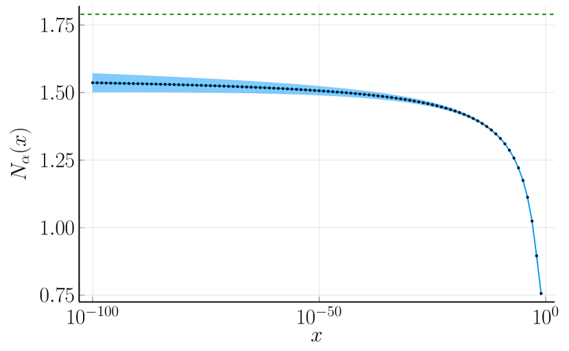
(b)

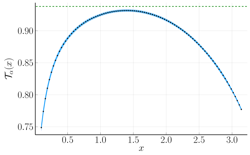
(c)

Figure 3: Plot of the functions $N_{\alpha}$ and $\mathcal{T}_{\alpha}$ for $\alpha\in I_{1}$. The dashed green lines show the upper bounds as given in Lemmas 12.1 and 12.3

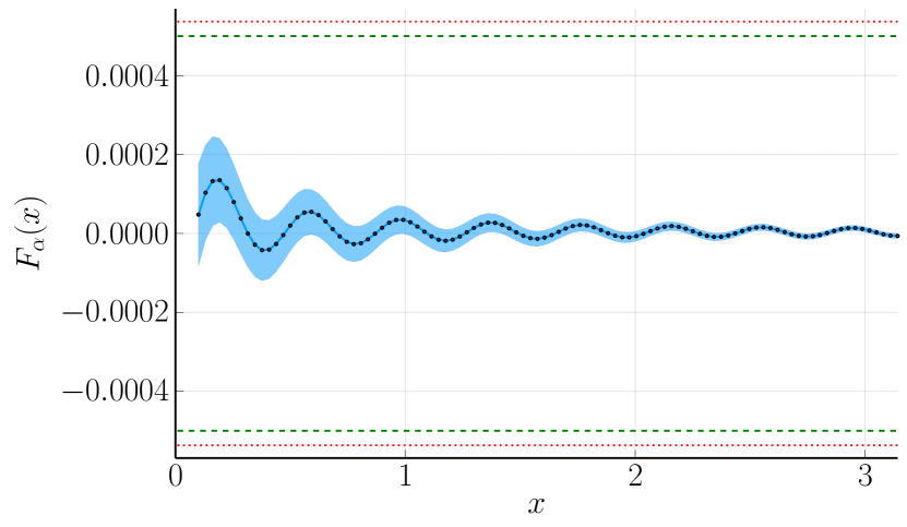
(a)

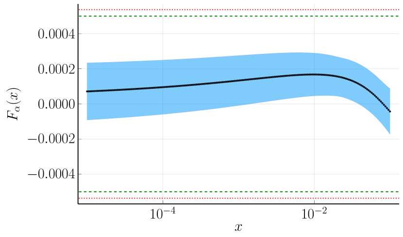
(b)

Figure 4: Plot of the function $F_{\alpha}$ for $\alpha\in I_{1}$. The function is plotted on the interval $[0,\pi]$ and $[10^{-5},10^{-1}]$. The dashed green line shows the upper bound as given in Lemma 12.2. The dotted red line shows $\frac{(1-\bar{D}_{1})^{2}}{4\bar{n}_{1}}$, which is the value we want $\delta_{\alpha}$ to be smaller than.

12.2 Bounds for $I_{2}$

We here give bounds of $n_{\alpha}$, $\delta_{\alpha}$ and $D_{\alpha}$ for $\alpha\in I_{2}=(-0.9999,-0.0012)$.

In this case it is not possible to give uniform bounds valid on the whole interval $I_{2}$. Instead we split $I_{2}$ into many subintervals and for each individual subinterval bounds are computed and they are checked to satisfy

$$\delta_{\alpha}<\frac{(1-D_{\alpha})^{2}}{4n_{\alpha}},$$

as required for Proposition 2.2.

When the midpoint of the subinterval is less than $-0.95$ the hybrid approach corresponding to $\alpha$ near $-1$ is used. In this case the weight is given by $w_{\alpha}(x)=|x|^{p}\log(2e+1/|x|)$. If the midpoint of the subinterval is larger than $-0.16$ then the hybrid approach corresponding to $\alpha$ near $0$ is used, in which case the weight is $w_{\alpha}(x)=|x|$. For the rest of the interval the default approach is used, with the weight $w_{\alpha}(x)=|x|^{p}$.

The value of $p$ is chosen based on the midpoint of the subinterval. If the midpoint is above $-0.33$ we use $p=1$ and if it is between $-0.5$ and $-0.33$ we use $p=\frac{3}{4}$. If it is below $-0.5$ we take $p=\frac{1-\alpha}{2}$, evaluated at the midpoint of the interval. Note that in all cases we have $-\alpha<p\leq 1$.

The interval is split into $72000$ subintervals. The sizes of the subintervals are smaller near $\alpha=-1$ and $\alpha=0$. The interval $(-0.9999,-0.0012)$ is first split non-uniformly into $32$ subintervals, each of these subintervals are then further split uniformly into a given number of subintervals, the number varying for the different parts, see Table 1. Of these $72000$ subintervals there are a few for which the computed bounds are too bad to satisfy the required inequality. This happens in $28$ cases, in all of these cases it is enough to bisect the subinterval once for the bounds to be good enough. The final result is therefore based on a total of $72028$ subintervals.

Interval	Subintervals	Interval	Subintervals
$[-0.9999,-0.999875]$	$500$	$[-0.7,-0.6]$	$1000$
$[-0.999875,-0.99985]$	$500$	$[-0.6,-0.5]$	$1500$
$[-0.99985,-0.9998]$	$1000$	$[-0.5,-0.45]$	$1000$
$[-0.9998,-0.9996]$	$1000$	$[-0.45,-0.41]$	$1000$
$[-0.9996,-0.9993]$	$1000$	$[-0.41,-0.37]$	$1000$
$[-0.9993,-0.999]$	$1000$	$[-0.37,-0.33]$	$1000$
$[-0.999,-0.998]$	$1000$	$[-0.33,-0.2]$	$10000$
$[-0.998,-0.996]$	$1000$	$[-0.2,-0.16]$	$3000$
$[-0.996,-0.993]$	$1000$	$[-0.16,-0.1]$	$500$
$[-0.993,-0.99]$	$1000$	$[-0.1,-0.05]$	$500$
$[-0.99,-0.95]$	$2000$	$[-0.05,-0.025]$	$500$
$[-0.95,-0.935]$	$5000$	$[-0.025,-0.0125]$	$1000$
$[-0.935,-0.9]$	$8000$	$[-0.0125,-0.00625]$	$2000$
$[-0.9,-0.85]$	$4000$	$[-0.00625,-0.003125]$	$4000$
$[-0.85,-0.8]$	$2000$	$[-0.003125,-0.0015625]$	$8000$
$[-0.8,-0.7]$	$2000$	$[-0.0015625,-0.0012]$	$4000$

Table 1: The interval $[-0.9999,-0.0012]$ is split into these $32$ subintervals which are then further split uniformly into the given number of subintervals. The first $11$ use the hybrid approach corresponding to $\alpha$ near $-1$ and the last $8$ use the hybrid approach corresponding to $\alpha$ near $0$, the ones in between use the default approach.

Due to the large number of subintervals, explicit bounds for each case is not given here, we refer to the repository [14] where the data can be found. The bounds are visualized in Figures 5(a), 5(b) and 5(c). However, these figures only give a rough picture since the number of subintervals is larger than the number of pixels in the picture and the subintervals are concentrated near $\alpha=-1$ and $\alpha=0$.

For the precise values of $N_{\alpha,0}$ and $N_{\alpha,1}$ we refer to the repository [14]. In general $N_{\alpha,0}$ takes it maximum value near $\alpha=-1$ and minimum value near $\alpha=0$, varying from $5799$ to $2$. For $N_{\alpha,1}$ it varies between $0$ and $16$.

The approach for bounding $n_{\alpha}$, $\delta_{\alpha}$ and $D_{\alpha}$ is given in the following three lemmas. The total runtime for the calculations on Dardel were around 12000 core hours (corresponding to a wall time of around 48 hours using 256 cores).

Lemma 12.5.

For all $\alpha\in I_{2}$ the value $N_{\alpha}$ is bounded. A sketch of the bound is given in Figure 5(a), for the precise bound for each value of $\alpha$ we refer to the repository [14].

Proof.

Similar to in Lemma 12.1 the maximum of $N_{\alpha}$ is in practice attained at $x=\pi$, which makes it easy to compute an accurate bound. As seen in the plot of $n_{\alpha}$ in Figure 5(a) it in general varies smoothly with $\alpha$, the exception being the points where the choice of weight is changed. We can also note that the bounds are well-behaved near $\alpha=-1$ and $\alpha=0$.

When computing the bounds the value of $\epsilon$ is not fixed, instead it is determined dynamically. Starting with $\epsilon=3$ we check if the asymptotic version of $N_{\alpha}$ evaluated at this point is less than $N_{\alpha}(\pi)$. if this is the case we take this value of $\epsilon$, otherwise we try with a slightly smaller $\epsilon$, stopping once we find one that works. On the interval $[0,\epsilon]$ we then check that $N_{\alpha}$ is bounded by $N_{\alpha}(\pi)$.

For the interval $[\epsilon,\pi]$ we compute an enclosure of the maximum.

In both cases we use Taylor expansions of degree $0$ when computing the bounds.

For the hybrid case when $\alpha$ is close to $-1$ the approach is exactly the same as above. For the hybrid case when $\alpha$ is close to $0$ we use the same approach as in Lemma 12.9 for computing a bound.

The computational time varies with $\alpha$, on average the computations took 4.05 seconds for each subinterval with a minimum and maximum of 0.018 and 144 seconds respectively. ∎

Lemma 12.6.

For all $\alpha\in I_{2}$ the value $\delta_{\alpha}$ is bounded. A sketch of the bound is given in Figure 5(b), for the precise bound for each value of $\alpha$ we refer to the repository [14].

Proof.

The value of $\delta_{\alpha}$ is heavily dependent on the precise approximation used. Very small changes in the approximation can give relatively large changes for $\delta_{\alpha}$. This is clearly seen in Figure 5(b) where the bound is seen to vary a lot from subinterval to subinterval. The patches where the bound is more or less continuous correspond to certain values of $N_{\alpha,0}$ in the approximation, when the value changes from one to the other it gives a large change in defect. There are also many isolated points where the bound is very different from the nearby points, this is mostly due to numerical instabilities when computing the coefficients for the approximation.

Similar to in the previous lemma the value of $\epsilon$ is not fixed but chosen dynamically. The precise choice is based on comparing the asymptotic and the non-asymptotic versions at different values and see where the asymptotic one starts to give tighter enclosures. The bounds on $[0,\epsilon]$ and $[\epsilon,\pi]$ are then computed separately, and their maximum is returned.

In both cases we use Taylor expansions, the degree is tuned depending on $\alpha$ and is between $2$ and $6$.

For the hybrid case when $\alpha$ is close to $-1$ the approach is exactly the same as above. For the hybrid case when $\alpha$ is close to $0$ some modifications needs to be made. For the interval $[0,\epsilon]$ we use Taylor models in $\alpha$ to compute enclosures for the coefficients in the expansion at $x=0$. Once we have the expansion we are able to compute Taylor expansions in $x$ of it, where we use degree $8$. For the interval $[\epsilon,\pi]$ we are not able to compute Taylor expansions in $x$ and have to fall back to using direct enclosures.

The computational time varies with $\alpha$, on average the computations took 37 seconds for each subinterval with a minimum and maximum of 0.11 and 1084 seconds respectively. ∎

Lemma 12.7.

For all $\alpha\in I_{2}$ the value $D_{\alpha}$ is bounded by a value smaller than $1$. A sketch of the bound is given in Figure 5(c), for the precise bound for each value of $\alpha$ we refer to the repository [14].

Proof.

The computation of the bound of $D_{\alpha}$ is the most time-consuming part. For that reason we do not attempt to compute a very accurate upper bound but only as much as we need for Lemma 12.8 to go through. We need $D_{\alpha}$ to satisfy the inequality

$$D_{\alpha}<1-2\sqrt{n_{\alpha}\delta_{\alpha}}.$$

Taking the upper bounds of $n_{\alpha}$ and $\delta_{\alpha}$ from the previous two lemmas we compute the value that $D_{\alpha}$ needs to be bounded by. To give a little headroom we subtract $2^{-26}$ to get the bound that we use. This bound is seen in Figure 5(c), and we prove that $D_{\alpha}$ is bounded by this value for all the subintervals.

To get an understanding of how this bound compares to the actual value of $D_{\alpha}$ we also compute a non-rigorous approximation of it. This approximation is computed by evaluating $\mathcal{T}_{\alpha}$ on a few points in the interval $[0,\pi]$ and taking the maximum, but with no control of what happens in between these points. This estimate can also be seen in Figure 5(c). From this estimate we can also compute an estimate of $\frac{(1-D_{\alpha})^{2}}{4n_{\alpha}}$, which is the value we want $\delta_{\alpha}$ to be less than, this estimate is seen in Figure 5(b).

Similar to in the previous two lemmas the value of $\epsilon$ is not fixed but chosen dynamically. It is determined by starting at $\epsilon=1$ and then taking smaller and smaller values until the asymptotic version of $\mathcal{T}_{\alpha}$ evaluated at $\epsilon$ satisfies the prescribed bound. We then prove that the bound holds on both $[0,\epsilon]$ and $[\epsilon,\pi]$.

For the interval $[0,\epsilon]$ we do not make use of Taylor expansions but only use direct evaluation. For the interval $[\epsilon,\pi]$ we are not able to compute Taylor expansion of $U_{\alpha}$, and hence not of $\mathcal{T}_{\alpha}$. We do however make one optimization to get better enclosures. Recall that

$$\mathcal{T}_{\alpha}(x)=\frac{U_{\alpha}(x)}{\pi|w_{\alpha}(x)||u_{\alpha}(x)|}.$$

For a given interval x both $U_{\alpha}(\textbf{{x}})$ and $w_{\alpha}(\textbf{{x}})$ are evaluated directly. To enclose $u_{\alpha}(\textbf{{x}})$ we first check if it is monotone by computing the derivative and checking that it is non-zero. If it is monotone we compute an enclosure by evaluating it at the endpoints of x.

Both the hybrid cases use exactly the same approach.

The computational time varies with $\alpha$, on average the computations took 72 seconds for each subinterval with a minimum and maximum of 0.740.68 and 1075 seconds respectively. ∎

Lemma 12.8.

For all $\alpha\in I_{2}$ the following inequality is satisfied

$$\delta_{\alpha}<\frac{(1-D_{\alpha})^{2}}{4n_{\alpha}}.$$

Proof.

Using the computed upper bounds from Lemma 12.5, 12.6 and 12.7 it is straight forward to check that the inequality

$$\delta_{\alpha}<\frac{(1-D_{\alpha})^{2}}{4n_{\alpha}}$$

holds for each of the $72028$ subintervals. Since the union of these subintervals cover the entire of $I_{2}$ it follows that the inequality holds for all $\alpha\in I_{2}$. ∎

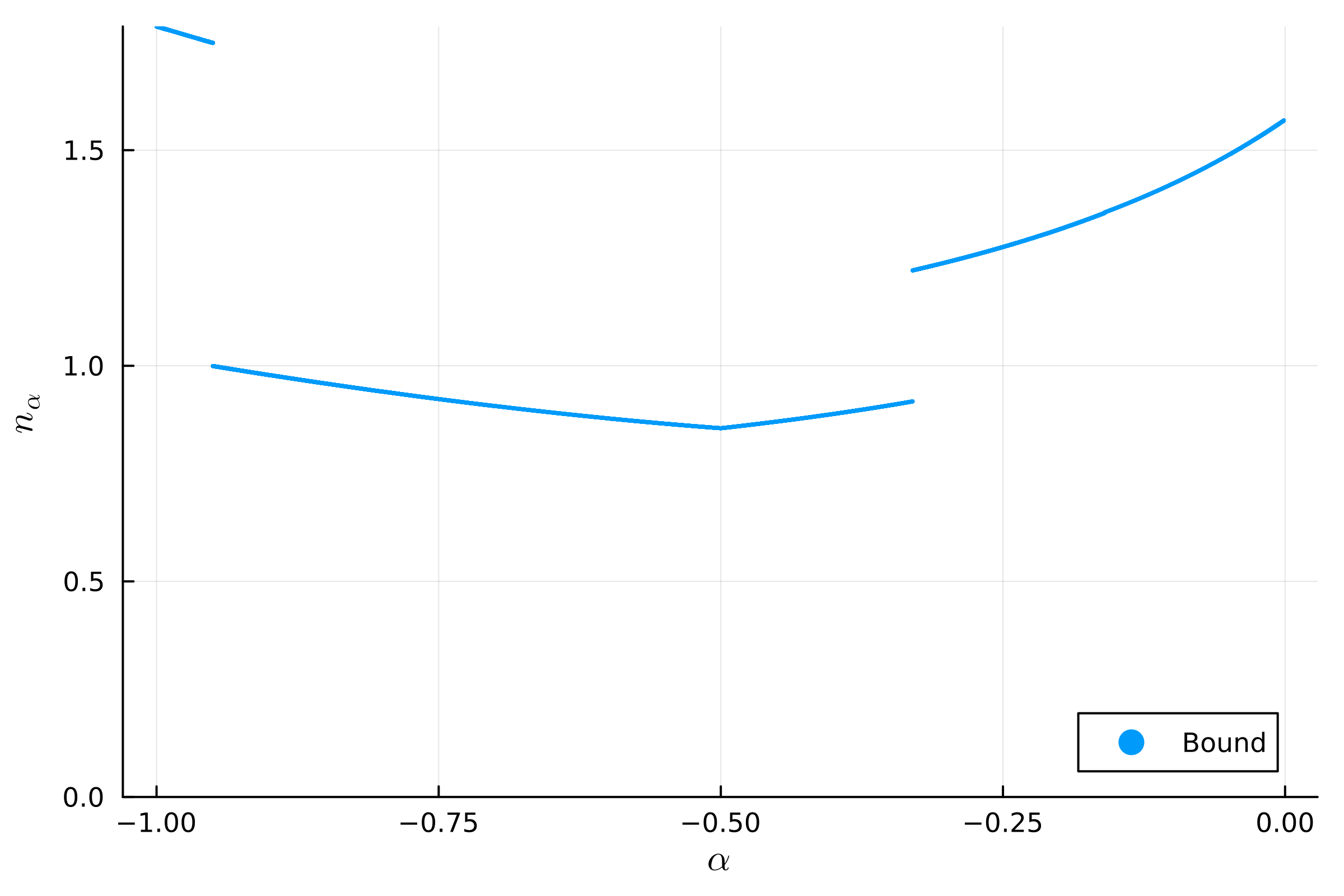
(a)

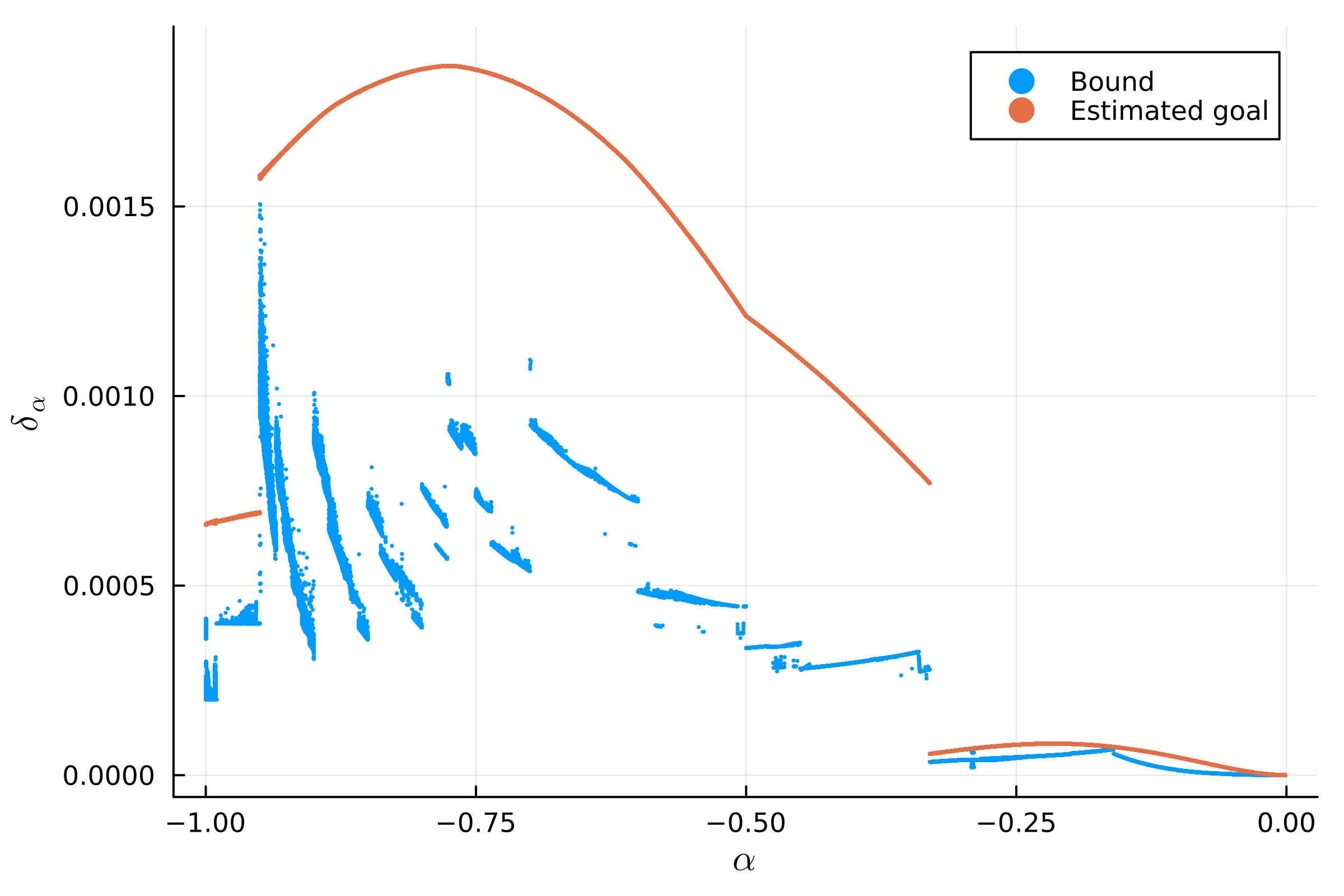
(b)

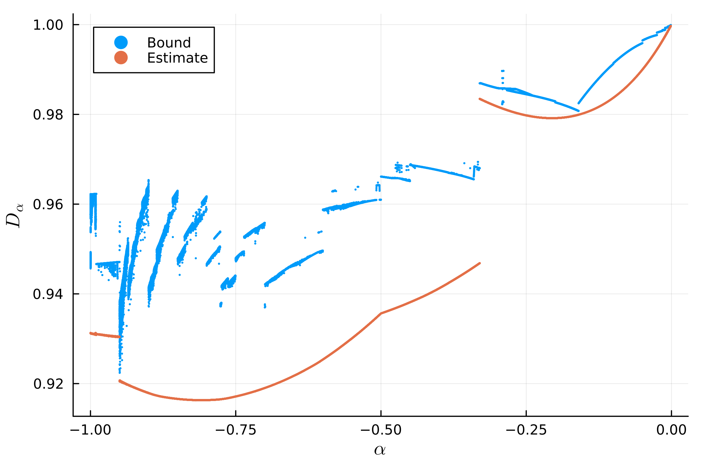
(c)

Figure 5: Plot of bounds of $n_{\alpha}$, $\delta_{\alpha}$ and $D_{\alpha}$ for $\alpha\in I_{2}$. For $\delta_{\alpha}$ the estimated goal is given by $\frac{(1-D_{\alpha})^{2}}{4n_{\alpha}}$ computed with the upper bound of $n_{\alpha}$ and the estimate of $D_{\alpha}$. For $D_{\alpha}$ the non-rigorous estimate is also included.

12.3 Bounds for $I_{3}$

For this interval the bounds are given in a slightly different form. As $\alpha$ gets close to $0$ the value of $\delta_{\alpha}$ tends to zero and $D_{\alpha}$ tends to one. To be able to say something about the inequality

$$\delta_{\alpha}<\frac{(1-D_{\alpha})^{2}}{4n_{\alpha}}$$

in Proposition 2.2 in the limit we therefore need information about the rate that they go to zero and one respectively. This is however not the case for $n_{\alpha}$, for which we have the following lemma:

Lemma 12.9.

The constant $n_{\alpha}$ satisfies the inequality $n_{\alpha}\leq\bar{n}_{3}=1.58$ for all $\alpha\in I_{3}$.

Proof.

A plot of $N_{\alpha}(x)$ on the interval $[0,\pi]$ is given in Figure 6(a), clearly hinting at the maximum being attained at $x=\pi$. We use the asymptotic expansion on the entire interval, i.e. $\epsilon=\pi$. The computation of the enclosure takes less than a second and gives us

$$n_{\alpha}\in[1.57\pm 2.45\cdot 10^{-3}],$$

which is upper bounded by $\bar{n}_{3}$. ∎

For $D_{\alpha}$ and $\delta_{\alpha}$ we give bounds which are functions of $\alpha$.

Lemma 12.10.

The constant $\delta_{\alpha}$ satisfies the inequality $\delta_{\alpha}\leq\bar{\Delta}_{\delta}\cdot\alpha^{2}$, where $\bar{\Delta}_{\delta}=0.0077$, for all $\alpha\in I_{3}$.

Proof.

For each $x\in[0,\pi]$ we can compute a Taylor model $M_{F}(x)$ of degree $1$ in $\alpha$ of $F_{\alpha}(x)$ centered at $\alpha=0$ and valid for $\alpha\in I_{3}$. This means that $M_{F}(x)$ satisfies

$$F_{\alpha}(x)\in p_{M_{F}(x)}(\alpha)+\Delta_{M_{F}(x)}\alpha^{2}$$

for all $\alpha\in I_{3}$, where $p_{M_{F}(x)}$ is the degree $1$ polynomial associated with the Taylor model and $\Delta_{M_{F}(x)}$ is the remainder. From Lemma 10.1 we get that $p_{M_{F}(x)}=0$ for all $x\in[0,\pi]$, hence

$$|F_{\alpha}(x)|\in|\Delta_{M_{F}(x)}|\alpha^{2}.$$

This gives us

$$\delta_{\alpha}=\sup_{x\in[0,\pi]}|F_{\alpha}(x)|\in\left(\sup_{x\in[0,\pi]}|\Delta_{M_{F}(x)}|\right)\alpha^{2}=:\Delta_{\delta}\alpha^{2},$$

where we with the supremum of intervals we mean the interval whose upper endpoint is the supremum of all upper endpoints and the lower endpoint is the supremum of all lower endpoints. A plot of $\Delta_{M_{F}(x)}$ on the interval $[0,\pi]$ is given in Figure 6(b), we are interested in enclosing $\Delta_{\delta}$.

We use the asymptotic expansion on the entire interval, i.e. $\epsilon=\pi$. Enclosing the supremum we get the interval

$$\Delta_{\delta}\subseteq[0,7.65\cdot 10^{-3}],$$

for which an upper bound is given by $\bar{\Delta}_{\delta}$. The runtime is around 3 seconds. ∎

Lemma 12.11.

The constant $D_{\alpha}$ satisfies the inequality $D_{\alpha}\leq 1+\bar{\Delta}_{D}\cdot\alpha$, where $\bar{\Delta}_{D}=0.226$, for all $\alpha\in I_{3}$.

Proof.

The proof is similar to the previous lemma. For each $x\in[0,\pi]$ we can compute a Taylor model $M_{\mathcal{T}}(x)$ of degree $0$ in $\alpha$ of $\mathcal{T}_{\alpha}(x)$ centered at $\alpha=0$ and valid for $\alpha\in I_{3}$. This means that $M_{\mathcal{T}}(x)$ satisfies

$$\mathcal{T}_{\alpha}(x)\in p_{M_{\mathcal{T}}(x)}(\alpha)+\Delta_{M_{\mathcal{T}}(x)}\alpha$$

for all $\alpha\in I_{3}$, where $p_{M_{\mathcal{T}}(x)}$ is the degree $0$ polynomial associated with the Taylor model and $\Delta_{M_{\mathcal{T}}(x)}$ is the remainder. From Lemma 11.8 we get that $p_{M_{\mathcal{T}}(x)}=1$ for all $x\in[0,\pi]$, hence

$$\mathcal{T}_{\alpha}(x)\in 1+\Delta_{M_{\mathcal{T}}(x)}\alpha.$$

This gives us

$$D_{\alpha}=\sup_{x\in[0,\pi]}|\mathcal{T}_{\alpha}(x)|\in 1+\left(\inf_{x\in[0,\pi]}\Delta_{M_{\mathcal{T}}(x)}\right)\alpha=:1+\Delta_{D}\alpha,$$

where we take the infimum since $\alpha$ is negative. A plot of $\Delta_{M_{\mathcal{T}}(x)}$ is given in Figure 6(c), we are interested in enclosing $\Delta_{D}$.

We take $\epsilon=1$. From Figure 6(c) it seems like the infimum is attained at $x=0$, we therefore compute the infimum on the interval $[0,\epsilon]$ first and then only prove that the value on $[\epsilon,\pi]$ is lower bounded by this. Enclosing the infimum on $[0,\epsilon]$ we get the enclosure

$$\Delta_{D}\subset[0.2413\pm 0.0151],$$

which is then checked to be a lower bound for $[\epsilon,\pi]$. This computed enclosure is then lower bounded by $\bar{\Delta}_{D}$. The runtime is around 7 seconds. ∎

Combining the above we get the following result.

Lemma 12.12.

For all $\alpha\in I_{3}$ the following inequality is satisfied

$$\delta_{\alpha}<\frac{(1-D_{\alpha})^{2}}{4n_{\alpha}}.$$

Proof.

From lemma 12.9 and 12.11 we get

$$\frac{(1-D_{\alpha})^{2}}{4n_{\alpha}}\geq\frac{\bar{\Delta}_{D}^{2}}{4\bar{n}_{3}}\cdot\alpha^{2}$$

for all $\alpha\in I_{3}$. Combining this with lemma 12.10 means we only have to check the inequality

$$\bar{\Delta}_{\delta}<\frac{\bar{\Delta}_{D}^{2}}{4\bar{n}_{3}},$$

which indeed holds. ∎

(a)

(b)

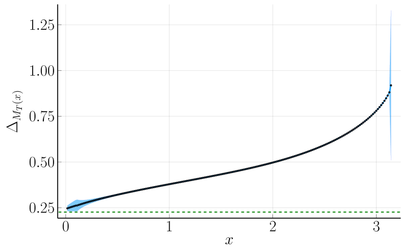
(c)

Figure 6: Plots for $\alpha\in I_{3}$. The leftmost figure shows a plot of $N_{\alpha}(x)$. The two other figures show enclosures of $\Delta_{M_{F}(x)}$ and $\Delta_{M_{\mathcal{T}}(x)}$, the remainder terms of the Taylor models for $F_{\alpha}(x)$ and $\mathcal{T}_{\alpha}(x)$ respectively. The dashed green lines shows the upper/lower bounds given in Lemmas 12.9, 12.10 and 12.11. The dotted red line in the middle figure shows $\frac{\bar{\Delta}_{D}^{2}}{4\bar{n}_{3}}$, the value that $\Delta_{\delta}$ needs to be smaller than.

13 Proof of Theorem 1.1

We are now ready to give the proof of Theorem 1.1.

Proof of Theorem 1.1.

Consider the operator $G_{\alpha}$ from (11) given by

$$G_{\alpha}[v]=(I-T_{\alpha})^{-1}(-F_{\alpha}-N_{\alpha}v^{2}).$$

Combining Lemmas 12.3, 12.7 and 12.11 we have $\|T_{\alpha}\|<1$ for all $\alpha\in(-1,0)$, so the inverse of the operator $I-T_{\alpha}$ is well-defined. Combining Lemmas  12.4, 12.8 and 12.12 gives us that the inequality

$$\delta_{\alpha}<\frac{(1-D_{\alpha})^{2}}{4n_{\alpha}}$$

holds for all $\alpha\in(-1,0)$. This, together with Proposition 2.2 and Banach fixed-point theorem, proves that for

$$\epsilon_{\alpha}=\frac{1-D_{\alpha}-\sqrt{(1-D_{\alpha})^{2}-4\delta_{\alpha}n_{\alpha}}}{2n_{\alpha}}$$

the operator $G_{\alpha}$ has a unique fixed-point $v_{\alpha}$ in $X_{\epsilon_{\alpha}}\subseteq L^{\infty}(\mathbb{T})$.

By the construction of the operator $G_{\alpha}$ this means that the function

$$u(x)=u_{\alpha}(x)+w_{\alpha}(x)v_{\alpha}(x)$$

solves (5), given by

$$\frac{1}{2}u^{2}=-\mathcal{H}^{\alpha}[u].$$

For any wave speed $c\in\mathbb{R}$ we then have that the function

$$\varphi(x)=c-u(x)$$

is a traveling wave solution to (1). This proves the existence of a $2\pi$-periodic highest cusped traveling wave.

The asymptotic behavior of $u_{\alpha}$ close to $x=0$ is given by

$$u_{\alpha}(x)=\nu_{\alpha}|x|^{-\alpha}+\mathcal{O}(|x|^{-\alpha+p_{\alpha}}).$$

with $\nu_{\alpha}$ as in Lemma 4.1. The precise value for $p_{\alpha}$ varies depending on the type of construction used, but in all cases it satisfies $-\alpha+p_{\alpha}>1$. Furthermore the weight satisfies

$$w_{\alpha}(x)=\mathcal{O}(|x|^{p})$$

for some $p$ with $-\alpha<p\leq 1$. Hence

$$u(x)=u_{\alpha}(x)+w_{\alpha}(x)v_{\alpha}(x)=\nu_{\alpha}|x|^{-\alpha}+\mathcal{O}(|x|^{p})$$

and

$$\varphi(x)=c-\nu_{\alpha}|x|^{-\alpha}+\mathcal{O}(|x|^{p}),$$

as we wanted to show. ∎

Appendix A Removable singularities

In several cases we have to compute enclosures of functions with removable singularities. For example the function

$$\Gamma(1-s)\cos(\pi(1-s)/2)$$

comes up when computing $C_{s}$ through equation (39) and has a removable singularity whenever $s$ is a positive even integer. For this we follow the same approach as in [15, Appendix A], where more details are given. The main tool is the following lemma:

Lemma A.1.

Let $m\in\mathbb{Z}_{\geq 0}$ and let $I$ be an interval containing zero. Consider a function $f(x)$ with a zero of order $n$ at $x=0$ and such that $f^{(m+n)}(x)$ is absolutely continuous on $I$. Then for all $x\in I$ we have

$$\frac{f(x)}{x^{n}}=\sum_{k=0}^{m}f_{k+n}(0)x^{k}+f_{m+n+1}(\xi)x^{m+1}$$

for some $\xi$ between $0$ and $x$. Furthermore, if $f^{m+n+p}(x)$ is absolutely continuous for $p\in\mathbb{Z}_{\geq 0}$ we have

$$\frac{d^{p}}{dx^{p}}\frac{f(x)}{x^{n}}=\sum_{k=0}^{m}\frac{(k+p)!}{k!}f_{k+n+p}(0)x^{k}+\frac{(m+p+1)!}{(m+1)!}f_{m+n+p+1}(\xi)x^{m+1}$$

for some $\xi$ between $0$ and $x$.

We also make use of the first statement of the lemma for $x\in\mathbb{C}$, the proof is the same as for $x\in\mathbb{R}$.

Appendix B Taylor models

An important tool for handling the limit $\alpha\to 0$ is the use of Taylor models for enclosing $\delta_{\alpha}$ and $D_{\alpha}$. We here give a brief introduction to Taylor models, for a more thorough introduction we refer to [44].

With a Taylor model we mean what in [44] is refereed to as a Taylor model with relative error. We use the following definition, compare with [44, Definition 2.3.2].

Definition B.1.

A Taylor model $M=(p,\Delta)$ of degree $n$ for a function $f$ on an interval $I$ centered at a point $x_{0}\in I$ is a polynomial $p$ of degree $n$ together with an interval $\Delta$, satisfying that for all $x\in I$ there is $\delta\in\Delta$ such that

$$f(x)-p(x-x_{0})=\delta(x-x_{0})^{n+1}.$$

For an $n+1$ times differentiable function $f$ the polynomial $p$ is the Taylor polynomial of degree $n$ of $f$ centered at $x_{0}$ [44, Lemma 2.3.3]. A Taylor model is thus given by a truncated Taylor expansion plus a bound on the remainder term valid on some interval $I$. From Taylor’s theorem we see that we can take $\Delta$ to be an enclosure of $\frac{f^{n+1}(x)}{(n+1)!}$ on the interval $I$.

We can perform arithmetic on Taylor models. Given two functions $f$ and $g$ with corresponding Taylor models $M_{f}=(p_{f},\Delta_{f})$ and $M_{g}=(p_{g}+\Delta_{g})$ we can compute a Taylor model of $f+g$ as $M_{f+g}=(p_{f}+p_{g},\Delta_{f}+\Delta_{g})$, similarly for $f-g$. With slightly more work we can compute a Taylor model of $f\cdot g$, see [44, Algorithm 2.3.6], as well as of $f/g$, see [44, Algorithm 2.3.12]. The division can directly handle removable singularities for $f/g$, if there is a removable singularity of order $k$ then we need Taylor models of degree $n+k$ for $f$ and $g$ to get a Taylor model of degree $n$ for $f/g$. We can also compose Taylor models with arbitrary functions, given a Taylor model $M_{f}$ of $f$ and a function $g$ we can compute a Taylor model $M_{g\circ f}$ of $g\circ f$, see [44, Algorithm 2.3.8].

B.1 Taylor models in $\alpha$ of expansions in $x$

For both $F_{\alpha}(x)$ and $\mathcal{T}_{\alpha}(x)$ we need to compute expansions in $x$ to evaluate them near $x=0$. For $\alpha\in I_{3}$ we then need to compute Taylor models in $\alpha$ from these expansions, see Section 10.3 and 11.2.3. This is done by computing Taylor models of the coefficients in the expansion in $x$.

For example, consider the problem of computing an expansion in $x$ of $u_{\alpha}(x)$, used e.g. when computing $\frac{x^{-\alpha}}{u_{\alpha}(x)}$. For $\alpha\in I_{3}$ we have from Lemma 4.2, and using that $N_{\alpha,1}=0$ in this case,

$$u_{\alpha}(x)=\sum_{j=0}^{N_{\alpha,0}}a_{\alpha,j}^{0}|x|^{-\alpha+jp_{\alpha}}+\sum_{m=1}^{\infty}\frac{(-1)^{m}}{(2m)!}\left(\sum_{j=1}^{N_{\alpha,0}}a_{\alpha,j}\zeta(1-\alpha+jp_{\alpha}-2m)\right)x^{2m}.$$

It is straight forward to compute Taylor models of the coefficients $a_{\alpha,j}^{0}$ and

$$\frac{(-1)^{m}}{(2m)!}\left(\sum_{j=1}^{N_{\alpha,0}}a_{\alpha,j}\zeta(1-\alpha+jp_{\alpha}-2m)\right).$$

for $m<M$. What remains is computing a Taylor model bounding the tail. To compute a Taylor model enclosing a sum of the form

$$\sum_{m=M}^{\infty}c_{\alpha,m}x^{2m}.$$

it is enough to have a method for enclosing

$$\frac{d^{k}}{d\alpha^{k}}\sum_{m=M}^{\infty}c_{\alpha,m}x^{2m}.$$

for $k\geq 0$. For the Clausen functions this is given in Lemma C.6.

B.2 Taylor model of $p_{\alpha}$

The above is enough to compute Taylor models of functions in the paper for which we have explicit expressions. For $p_{\alpha}$ from (17) we only have an implicit equation defining it, and we have to take a slightly different approach.

Consider the equation

$$f(x,y)=0.$$

We want to compute a Taylor model of $y=y(x)$. Consider a Taylor model of degree $n$, centered at $x_{0}$ and which should be valid on the interval $I$. As mentioned above it is enough to compute the Taylor polynomial of $y(x)$ at $x=x_{0}$ of degree $n$ and enclose $\frac{y^{n+1}(x)}{(n+1)!}$ on $I$.

Let $y_{0}$ be such that $f(x_{0},y_{0})=0$. We first consider the case when $f_{y}(x_{0},y_{0})\not=0$. If $f$ is sufficiently smooth we can use the implicit function theorem to compute a Taylor polynomial of $y$ at $x_{0}$ to degree $n$. Expanding $f(x,y(x))$ at $x_{0}$ we get

$$f(x_{0},y_{0})+(f_{x}(x_{0},y_{0})+y^{\prime}(x_{0})f_{y}(x_{0},y_{0}))(x-x_{0})\\ +\frac{1}{2}(f_{xx}(x_{0},y_{0})+2y^{\prime}(x_{0})f_{xy}(x_{0},y_{0})+y^{\prime}(x_{0})f_{yy}(x_{0},y_{0})+y^{\prime\prime}(x_{0})f_{y}(x_{0},y_{0}))(x-x_{0})^{2}\cdots=0.$$

Solving for $y^{\prime}(x_{0})$, $y^{\prime\prime}(x_{0})$, etc., we get

$$y^{\prime}(x_{0}) =\frac{f_{x}(x_{0},y(x_{0}))}{f_{y}(x_{0},y(x_{0}))},$$

$$y^{\prime\prime}(x_{0}) =\frac{f_{xx}(x_{0},y_{0})+2y^{\prime}(x_{0})f_{xy}(x_{0},y_{0})+y^{\prime}(x_{0})f_{yy}(x_{0},y_{0})}{2f_{y}(x_{0},y(x_{0}))}$$

and similarly for higher orders.

While it is possible to use the above formulas for the derivatives to enclose $\frac{y^{n+1}(x)}{(n+1)!}$ on $I$ this gets very complicated for $p_{\alpha}$ at $\alpha=0$ due to the large number of removable singularities to handle. Instead, we take a slightly different, more direct, approach for computing $\Delta$. We want to find $\Delta$ such that for all $x\in I$ there is $\delta\in\Delta$ such that

$$f(x,p(x-x_{0})+\delta(x-x_{0})^{n+1})=0.$$

If we let

$$g(x,\delta)=f(x,p(x-x_{0})+\delta(x-x_{0})^{n+1})$$

we want $\Delta$ to be an enclosure of a root in $\delta$ of $g$ for all $x\in I$. To make the derivative in $\delta$ non-zero at $x=x_{0}$ we normalize $g$ as

$$h(x,\delta)=\frac{g(x,\delta)}{(x-x_{0})^{n+1}}.$$

Given a guess $\Delta=[\underline{\Delta},\overline{\Delta}]$, to prove that this is an enclosure of a root we only need to verify that $h(x,\underline{\Delta})$ and $h(x,\overline{\Delta})$ both have constant signs for all $x\in I$ and that the two signs are different. The guess for $\Delta$ can be given using non-rigorous means, for example by looking at the error at the endpoints of $I$. Only the verification of the signs at the endpoints of $\Delta$ needs to be done rigorously.

For $p_{\alpha}$ we get from (17) the function

$$f(\alpha,p)=\frac{\Gamma(2\alpha-p)\cos\left(\frac{\pi}{2}(2\alpha-p)\right)}{\Gamma(\alpha-p)\cos\left(\frac{\pi}{2}(\alpha-p)\right)}-\frac{2\Gamma(2\alpha)\cos(\pi\alpha)}{\Gamma(\alpha)\cos\left(\frac{\pi}{2}\alpha\right)}.$$

In this case $\alpha=0$ we have $f_{p}(0,p_{0})=0$, and we cannot apply the above approach directly. For the coefficients of polynomial of the Taylor model we expand

$$f(\alpha,p_{0}+p_{1}\alpha+p_{2}\alpha^{2})$$

at $\alpha=0$. The constant coefficient is exactly zero, and we then solve for $p_{0}$, $p_{1}$ and $p_{2}$ making the three coming coefficients zero. For the remainder term of the Taylor model we instead we consider the function $\frac{f(\alpha,p)}{\alpha}$, for which the above approach does work.

Appendix C Computing Clausen functions

To be able to compute bounds of $D_{\alpha}$, $\delta_{\alpha}$ and $n_{\alpha}$ it is critical that we can compute accurate enclosures of $C_{s}(x)$ and $S_{s}(x)$, including expansions in the argument and derivatives in the parameter. For this we follow the same approach as in [15, Appendix B] with a few additions and improvements. We here give a shortened version of the approach while highlighting the additions and improvements.

We start by going through how to compute $C_{s}(x)$ and $S_{s}(x)$ for $s,x\in\mathbb{R}$. Since both $C_{s}(x)$ and $S_{s}(x)$ are $2\pi$-periodic we can reduce it to $x=0$ or $0<x<2\pi$.

For $x=0$ and $s>1$ have $C_{s}(0)=\zeta(s)$ and $S_{s}(0)=0$. For $s\leq 1$ both functions typically diverge at $x=0$.

For $0<x<2\pi$ we can compute the Clausen functions by going through the polylog function,

$$C_{s}(x)=\operatorname{Re}\left(\operatorname{Li}_{s}(e^{ix})\right),\quad S_{s}(x)=\operatorname{Im}\left(\operatorname{Li}_{s}(e^{ix})\right).$$

However it is computationally beneficial to instead go through the periodic zeta function [18, Sec. 25.13],

$$F(x,s):=\operatorname{Li}_{s}(e^{2\pi ix})=\sum_{n=1}^{\infty}\frac{e^{2\pi inx}}{n^{s}},$$

for which we have

$$C_{s}(x)=\operatorname{Re}F\left(\frac{x}{2\pi},s\right),\quad S_{s}(x)=\operatorname{Im}F\left(\frac{x}{2\pi},s\right).$$

Using [18, Eq. 25.13.2] we get, for $0<x<2\pi$,

$$C_{s}(x) =\frac{\Gamma(1-s)}{(2\pi)^{1-s}}\cos(\pi(1-s)/2)\left(\zeta\left(1-s,\frac{x}{2\pi}\right)+\zeta\left(1-s,1-\frac{x}{2\pi}\right)\right),$$ (39)

$$S_{s}(x) =\frac{\Gamma(1-s)}{(2\pi)^{1-s}}\sin(\pi(1-s)/2)\left(\zeta\left(1-s,\frac{x}{2\pi}\right)-\zeta\left(1-s,1-\frac{x}{2\pi}\right)\right).$$ (40)

This formulation works well as long as $s$ is not a non-negative integer. For non-negative integers we have to handle some removable singularities, for details see [15, Appendix B].

Compared to [15] we also need to compute $C_{s}(x)$ for real $s$ but complex $x$ during the rigorous integration discussed in Appendix D In those cases $s$ is never an integer, and we use Equation (39) which holds for $0<\operatorname{Re}x<2\pi$.

C.1 Interval arguments

Let $\textbf{{x}}=[\underline{x},\overline{x}]$ and $\textbf{{s}}=[\underline{s},\overline{s}]$ be two finite intervals, we are interested in computing an enclosure of $C_{\textbf{{s}}}(\textbf{{x}})$ and $S_{\textbf{{s}}}(\textbf{{x}})$. Due to the periodicity we can reduce it to three different cases for x

1. x doesn’t contain a multiple of $2\pi$, by adding or subtracting a suitable multiple of $2\pi$ we can assume that $0<\textbf{{x}}<2\pi$;

2. x has a diameter of at least $2\pi$, it then covers a full period and can without loss of generality be taken as $\textbf{{x}}=[0,2\pi]$;

3. x contains a multiple of $2\pi$ but has a diameter less than $2\pi$, by adding or subtracting a suitable multiple of $2\pi$ we can take x such that $-2\pi<\underline{x}\leq 0\leq\overline{x}<2\pi$.

The second and third case are handled exactly as in [15], for the first case we make some minor improvements.

For $C_{s}$ we make use of the following lemma which is a slightly upgraded version of [15, Lemma B.1], see also [22, Lemma B.1].

Lemma C.1.

For all $s\in\mathbb{R}$ the Clausen function $C_{s}(x)$ is monotone in $x$ on the interval $(0,\pi)$. For $s>0$ it is decreasing. For $s\leq 0$ the sign of the derivative is the same as that of $-\sin\left(\frac{\pi}{2}s\right)$.

Proof.

The derivative in $x$ is given by $-S_{s-1}(x)$. For $s>1$ the proof is the same as in [15, Lemma B.1].

For $s<1$ we use equation (40) together with [18, Eq. 25.11.25] to get

$$S_{s-1}(x)=\frac{\sin\left(\frac{\pi}{2}(2-s)\right)}{(2\pi)^{2-s}}\int_{0}^{\infty}t^{1-s}e^{-\frac{xt}{2\pi}}\frac{1-e^{(x/\pi-1)t}}{1-e^{-t}}\ dt,$$

which sign depends only on the value $s$ and is the same as that of $\sin\left(\frac{\pi}{2}s\right)$. In particular, for $0<s<1$ we have $\sin\left(\frac{\pi}{2}s\right)>0$ so $C_{s}(x)$ is decreasing for $0<s<1$.

For $s=1$ the result follows directly from that $C_{1}(x)=-\log(2\sin(x/2))$ on the interval. ∎

For $S_{s}$ we have the following, slightly weaker, result

Lemma C.2.

For $s\leq 1$ the Clausen function $S_{s}(x)$ is monotone in $x$ on the interval $(0,2\pi)$. The sign of the derivative is the same as that of $-\cos\left(\frac{\pi}{2}s\right)$.

Proof.

The derivative in $x$ is given by $C_{s-1}(x)$. For $s<1$ we use equation (39) together with [18, Eq. 25.11.25] to get

$$C_{s-1}(x)=\frac{\cos\left(\frac{\pi}{2}(2-s)\right)}{(2\pi)^{2-s}}\int_{0}^{\infty}t^{1-s}e^{-\frac{xt}{2\pi}}\frac{1+e^{(x/\pi-1)t}}{1-e^{-t}}\ dt,$$

which sign depends only on the value $s$ and is the same as that of $-\cos\left(\frac{\pi}{2}s\right)$.

For $s=1$ the result follows directly from that $S_{1}(x)=\frac{\pi}{2}-\frac{x}{2}$ on the interval. ∎

For $s\leq 1$ the extrema of $S_{s}(\textbf{{x}})$ are thus always attained at $x=\underline{x}$ and $\overline{x}$. We handle $s>1$ by computing and enclosure of the derivative $S_{\textbf{{s}}}^{\prime}(\textbf{{x}})=C_{\textbf{{s}}-1}(\textbf{{x}})$, if the enclosure of the derivative doesn’t contain zero then the function is monotone, and we evaluate it at the endpoints, if the derivative contains zero we instead use the midpoint approximation $S_{\textbf{{s}}}(\textbf{{x}})=S_{\textbf{{s}}}(x_{0})+(\textbf{{x}}-x_{0})C_{\textbf{{s}}-1}(\textbf{{x}})$ where $x_{0}$ is the midpoint of x.

For s we follow the same approach as in [15]. The only difference is that we also have to handle s overlapping $1$, in which case the implementation of the deflated zeta function,

$$\underline{\zeta}(s,x)=\zeta(s,x)+\frac{1}{1-s}=\sum_{n=0}^{\infty}\frac{(-1)^{n}}{n!}\gamma_{n}(x)(s-1)^{n},$$ (41)

in Arb does not work directly. It only supports $s$ exactly equal to $1$, and not intervals containing $1$. Looking at the implementation it is however fairly easy to adapt it to also work for intervals containing $1$, which we have done.

C.2 Expansion in $x$

We now go through how to compute expansions of the Clausen functions in the argument $x$. In general the procedure is the same as in [15], except that we also have to handle the case when $s$ overlaps positive integers for the expansion at $x=0$.

At $x=0$ we have the following asymptotic expansions [22]

$$C_{s}(x) =\Gamma(1-s)\sin\left(\frac{\pi}{2}s\right)|x|^{s-1}+\sum_{m=0}^{\infty}(-1)^{m}\zeta(s-2m)\frac{x^{2m}}{(2m)!};$$ (42)

$$S_{s}(x) =\Gamma(1-s)\cos\left(\frac{\pi}{2}s\right)\operatorname{sgn}(x)|x|^{s-1}+\sum_{m=0}^{\infty}(-1)^{m}\zeta(s-2m-1)\frac{x^{2m+1}}{(2m+1)!}.$$ (43)

For positive integers we have to handle the poles of $\Gamma(s)$ at non-positive integers and the pole of $\zeta(s)$ at $s=1$.

For $C_{s}(x)$ with positive even integers $s$ the only problematic term is

$$\Gamma(1-s)\sin\left(\frac{\pi}{2}s\right)|x|^{s-1}$$

which has a removable singularity. Similarly, for $S_{s}(x)$ with positive odd integers $s$. For $C_{s}(x)$ with positive odd integers $s$ and $S_{s}$ with positive even integers $s$ the singularities are not removable. The only case we encounter in the paper is for $C_{s}$, for which we make use of the following lemma to bound the sum of the two singular terms.

Lemma C.3.

Let $m\geq 1$ and $s\in\left[2m+\frac{1}{2},2m+\frac{3}{2}\right]$, then

$$\Gamma(1-s)\sin\left(\frac{\pi}{2}s\right)|x|^{s-1}+(-1)^{m}\zeta(s-2m)\frac{x^{2m}}{(2m)!}=K_{1}|x|^{s-1}+K_{2}x^{2m}+K_{3}x^{2m}\frac{|x|^{s-(2m+1)}-1}{s-(2m+1)}$$

with

$$K_{1} =\frac{\frac{\Gamma(2m+2-s)}{(1-s)_{2m}}\sin\left(\frac{\pi}{2}s\right)-\frac{(-1)^{m}}{(2m!)}}{2m+1-s},$$

$$K_{2} =-\frac{(-1)^{m}\underline{\zeta}(s-2m)}{(2m)!},$$

$$K_{3} =-\frac{(-1)^{m}}{(2m)!}.$$

Proof.

The result follows directly from adding and subtracting

$$(-1)^{m}\frac{|x|^{s-1}}{(2m+1-s)(2m)!}$$

and collecting the terms. ∎

Computing $K_{2}$ and $K_{3}$ is straight forward, for $K_{1}$ there is a removable singularity to handle. The function

$$x^{2m}\frac{|x|^{s-(2m+1)}-1}{s-(2m+1)}$$

also has a removable singularity, to compute an accurate enclosure we use the following lemma.

Lemma C.4.

For $x\not=0$ the function

$$\frac{|x|^{t}-1}{t}$$

is non-decreasing in $t$. In the limit $t\to 0$ it is equal to $\log|x|$.

Proof.

The derivative in $t$ is given by

$$\frac{1+(t\log|x|-1)|x|^{t}}{t^{2}}.$$ (44)

The sign depends on the numerator, which we can write as

$$1+(t\log|x|-1)e^{t\log|x|}.$$

Letting $v=t\log|x|$ we can write this as $1+(v-1)e^{v}$, which has the unique root $v=0$ and is positive for other values of $v$. It follows that (44) is non-negative and hence the function non-decreasing.

For the limit $t\to 0$ we directly get

$$\lim_{t\to 0}\frac{|x|^{t}-1}{t}=\lim_{t\to 0}\frac{\log|x|\ |x|^{t}}{1}=\log|x|.$$

∎

These two lemmas are only strictly required for interval s overlapping positive odd integers. However, it gives better enclosures also when s is close to such integers, even if it doesn’t overlap them. This is used to compute better enclosures in some cases.

The tails for the asymptotic expansions are bounded using the following lemma, see also [22, Lemma 2.1]. We omit the proof since it is very similar to that in [22].

Lemma C.5.

Let $s\geq 0$, $2M\geq s+1$ and $|x|<2\pi$, we then have the following bounds for the tails in equations (42) and (43)

$$\left|\sum_{m=M}^{\infty}(-1)^{m}\zeta(s-2m)\frac{x^{2m}}{(2m)!}\right| \leq 2(2\pi)^{1+s-2M}\left|\sin\left(\frac{\pi}{2}s\right)\right|\zeta(2M+1-s)\frac{x^{2M}}{4\pi^{2}-x^{2}},$$

$$\left|\sum_{m=M}^{\infty}(-1)^{m}\zeta(s-2m-1)\frac{x^{2m+1}}{(2m+1)!}\right| \leq 2(2\pi)^{s-2M}\left|\cos\left(\frac{\pi}{2}s\right)\right|\zeta(2M+2-s)\frac{x^{2M+1}}{4\pi^{2}-x^{2}}.$$

C.3 Derivatives in $s$

For $C_{s}^{(\beta)}(x)$ and $S_{s}^{(\beta)}(x)$ we use (39) and (40) and differentiate directly in $s$. When $s$ is not an integer this is handled directly using Taylor arithmetic, for integers we use the approach in Appendix A to handle the removable singularities.

To get asymptotic expansions at $x=0$ we take the expansions (42) and (43) and differentiate them with respect to $s$. Giving us

$$C_{s}^{(\beta)}(x) =\frac{d}{ds^{\beta}}\left(\Gamma(1-s)\sin\left(\frac{\pi}{2}s\right)|x|^{s-1}\right)+\sum_{m=0}^{\infty}(-1)^{m}\zeta^{(\beta)}(s-2m)\frac{x^{2m}}{(2m)!};$$ (45)

$$S_{s}^{(\beta)}(x) =\frac{d}{ds^{\beta}}\left(\Gamma(1-s)\cos\left(\frac{\pi}{2}s\right)\operatorname{sgn}(x)|x|^{s-1}\right)+\sum_{m=0}^{\infty}(-1)^{m}\zeta^{(\beta)}(s-2m-1)\frac{x^{2m+1}}{(2m+1)!}.$$ (46)

These formulas work well when $s$ is not a positive odd integer for $C_{s}^{(\beta)}(x)$ or a positive even integer for $S_{s}^{(\beta)}(x)$, and the derivatives can be computed using Taylor expansions. We mostly make use of the functions $C_{2}^{(1)}(x)$ and $C_{3}^{(1)}(x)$, in which case the expansions can be computed explicitly using [3, Eq. 16], for $|x|<2\pi$ we have

$$C_{2}^{(1)}(x)= \zeta^{(1)}(2)-\frac{\pi}{2}|x|\log|x|-(\gamma-1)\frac{\pi}{2}|x|+\sum_{m=1}^{\infty}(-1)^{m}\zeta^{(1)}(2-2m)\frac{x^{2m}}{(2m)!}$$

$$C_{3}^{(1)}(x)= \zeta^{(1)}(3)-\frac{1}{4}x^{2}\log^{2}|x|+\frac{3-2\gamma}{4}x^{2}\log|x|-\frac{36\gamma-12\gamma^{2}-24\gamma_{1}-42+\pi^{2}}{48}x^{2}$$

$$+\sum_{m=2}^{\infty}(-1)^{m}\zeta^{(1)}(3-2m)\frac{x^{2m}}{(2m)!}.$$

Where $\gamma_{n}$ is the Stieltjes constant and $\gamma=\gamma_{0}$. To bound the tails we have the following lemma from [15].

Lemma C.6.

Let $\beta\geq 1$, $s\geq 0$, $2M\geq s+1$ and $|x|<2\pi$, we then have the following bounds:

$$\left|\sum_{m=M}^{\infty}(-1)^{m}\zeta^{(\beta)}(s-2m)\frac{x^{2m}}{(2m)!}\right|\\ \leq\sum_{j_{1}+j_{2}+j_{3}=\beta}\binom{\beta}{j_{1},j_{2},j_{3}}2\left(\log(2\pi)+\frac{\pi}{2}\right)^{j_{1}}(2\pi)^{s-1}|\zeta^{(j_{3})}(1+2M-s)|\sum_{m=M}^{\infty}\left|p_{j_{2}}(1+2m-s)\left(\frac{x}{2\pi}\right)^{2m}\right|,$$

$$\left|\sum_{m=M}^{\infty}(-1)^{m}\zeta^{(\beta)}(s-2m-1)\frac{x^{2m+1}}{(2m+1)!}\right|\\ \leq\sum_{j_{1}+j_{2}+j_{3}=\beta}\binom{\beta}{j_{1},j_{2},j_{3}}2\left(\log(2\pi)+\frac{\pi}{2}\right)^{j_{1}}(2\pi)^{s-2}|\zeta^{(j_{3})}(2+2M-s)|\sum_{m=M}^{\infty}\left|p_{j_{2}}(2+2m-s)\left(\frac{x}{2\pi}\right)^{2m+1}\right|.$$

Here $p_{j_{2}}$ is given recursively by

$$p_{k+1}(s)=\psi^{(0)}(s)p_{k}(s)+p^{\prime}_{k}(s),\quad p_{0}=1,$$

where $\psi^{(0)}$ is the polygamma function. It is given by a linear combination of terms of the form

$$(\psi^{(0)}(s))^{q_{0}}(\psi^{(1)}(s))^{q_{1}}\cdots(\psi^{(j_{2}-1)}(s))^{q_{j_{2}-1}}.$$

We have the following bounds

$$\sum_{m=M}^{\infty}\left|(\psi^{(0)}(1+2m-s))^{q_{0}}\cdots(\psi^{(j_{2}-1)}(1+2m-s))^{q_{j_{2}-1}}\left(\frac{x}{2\pi}\right)^{2m}\right|\\ \leq|(\psi^{(1)}(1+2M-s))^{q_{1}}\cdots(\psi^{(j_{2}-1)}(1+2M-s))^{q_{j_{2}-1}}|\frac{1}{2^{q_{0}/2}}(2\pi)^{-2M}\Phi\left(\frac{x^{2}}{4\pi^{2}},-\frac{q_{0}}{2},M+\frac{1}{2}\right)x^{2M}$$

and

$$\sum_{m=M}^{\infty}\left|(\psi^{(0)}(2+2m-s))^{q_{0}}\cdots(\psi^{(j_{2}-1)}(2+2m-s))^{q_{j_{2}-1}}\left(\frac{x}{2\pi}\right)^{2m+1}\right|\\ \leq|(\psi^{(1)}(2+2M-s))^{q_{1}}\cdots(\psi^{(j_{2}-1)}(2+2M-s))^{q_{j_{2}-1}}|\frac{1}{2^{q_{0}/2}}(2\pi)^{-2M-1}\Phi\left(\frac{x^{2}}{4\pi^{2}},-\frac{q_{0}}{2},M+1\right)x^{2M+1}$$

where

$$\Phi(z,s,a)=\sum_{m=0}^{\infty}\frac{z^{m}}{(a+m)^{s}},$$

is the Lerch transcendent.

For $\alpha\in I_{1}$ the expansions in $x$ of $u_{\alpha}$ and $\mathcal{H}^{\alpha}[u_{\alpha}]$ are given in Lemma 4.6. Bounding the remainder terms for the sums

$$\sum_{m=1}^{\infty}\frac{(-1)^{m}}{(2m)!}a_{\alpha,0}\left(\zeta(1-\alpha-2m)-\zeta(2+(1+\alpha)^{2}/2-2m)\right)x^{2m}$$

and

$$\sum_{m=2}^{\infty}\frac{(-1)^{m}}{(2m)!}a_{\alpha,0}\left(\zeta(1-2\alpha-2m)-\zeta(2-\alpha+(1+\alpha)^{2}/2-2m)\right)x^{2m}$$

requires a bound similar to that in Lemma C.6 above. Factoring out $a_{\alpha,0}(1+\alpha)$, which is bounded, we are left bounding

$$\sum_{m=1}^{\infty}\frac{(-1)^{m}}{(2m)!}\frac{\zeta(1-\alpha-2m)-\zeta(2+(1+\alpha)^{2}/2-2m)}{1+\alpha}x^{2m}$$

and

$$\sum_{m=2}^{\infty}\frac{(-1)^{m}}{(2m)!}\frac{\zeta(1-2\alpha-2m)-\zeta(2-\alpha+(1+\alpha)^{2}/2-2m)}{1+\alpha}x^{2m}.$$

The following lemma allows us to write them in a form similar to that in Lemma C.6.

Lemma C.7.

For $-1<\alpha<0$ and $M_{1}\geq 1$ we have

$$\left|\sum_{m=M_{1}}^{\infty}\frac{(-1)^{m}}{(2m)!}\frac{\zeta(1-\alpha-2m)-\zeta(2+(1+\alpha)^{2}/2-2m)}{1+\alpha}x^{2m}\right|\\ \leq\left|\sum_{m=M_{1}}^{\infty}\frac{(-1)^{m}}{(2m)!}\zeta^{\prime}(s_{1,m}-2m)x^{2m}\right|+\frac{1+\alpha}{2}\left|\sum_{m=M_{1}}^{\infty}\frac{(-1)^{m}}{(2m)!}\zeta^{\prime}(s_{2,m}-2m)x^{2m}\right|$$

with $s_{1,m}\in[1-\alpha,2]$ and $s_{2,m}\in[2,2+(1+\alpha)^{2}/2]$. Similarly, for $M_{2}\geq 2$,

$$\left|\sum_{m=M_{2}}^{\infty}\frac{(-1)^{m}}{(2m)!}\frac{\zeta(1-2\alpha-2m)-\zeta(2-\alpha+(1+\alpha)^{2}/2-2m)}{1+\alpha}x^{2m}\right|\\ \leq 2\left|\sum_{m=M_{2}}^{\infty}\frac{(-1)^{m}}{(2m)!}\zeta^{\prime}(s_{3,m}-2m)x^{2m}\right|+\left(1-\frac{1+\alpha}{2}\right)\left|\sum_{m=M_{2}}^{\infty}\frac{(-1)^{m}}{(2m)!}\zeta^{\prime}(s_{4,m}-2m)x^{2m}\right|$$

with $s_{3,m}\in[1-2\alpha,3]$ and $s_{4,m}\in[2-\alpha+(1+\alpha)^{2}/2,3]$.

Proof.

The first inequality follows directly from that

$$\frac{\zeta(1-\alpha-2m)-\zeta(2+(1+\alpha)^{2}/2-2m)}{1+\alpha}=\frac{\zeta(1-\alpha-2m)-\zeta(2-2m)}{1+\alpha}+\frac{\zeta(2-2m)-\zeta(2+(1+\alpha)^{2}/2-2m)}{1+\alpha}$$

together with

$$\frac{\zeta(1-\alpha-2m)-\zeta(2-2m)}{1+\alpha}=\zeta^{\prime}(s_{1,m}-2m)$$

for some $s_{1,m}\in[1-\alpha,2]$ and

$$\frac{\zeta(2-2m)-\zeta(2+(1+\alpha)^{2}/2-2m)}{1+\alpha}=\frac{1+\alpha}{2}\zeta^{\prime}(s_{2,m}-2m)$$

for some $s_{2,m}\in[2,2+(1+\alpha)^{2}/2]$. The second one is similar. ∎

Lemma C.6 cannot be directly applied to the result of the above lemma since the argument of the zeta function depends on $m$. This can however be fixed, as the following lemma shows.

Lemma C.8.

Let $\beta\geq 1$, $\textbf{{s}}=[\underline{s},\overline{s}]$ with $\underline{s}\geq 0$, $2M\geq\overline{s}+1$, $s_{m}\in\textbf{{s}}$ for $m\geq M$ and $|x|<2\pi$, we then have the following bounds:

$$\left|\sum_{m=M}^{\infty}(-1)^{m}\zeta^{(\beta)}(s_{m}-2m)\frac{x^{2m}}{(2m)!}\right|\\ \leq\sum_{j_{1}+j_{2}+j_{3}=\beta}\binom{\beta}{j_{1},j_{2},j_{3}}2\left(\log(2\pi)+\frac{\pi}{2}\right)^{j_{1}}(2\pi)^{\overline{s}-1}|\zeta^{(j_{3})}(1+2M-\overline{s})|\sum_{m=M}^{\infty}\left|p_{j_{2}}(1+2m-s_{m})\left(\frac{x}{2\pi}\right)^{2m}\right|,$$

$$\left|\sum_{m=M}^{\infty}(-1)^{m}\zeta^{(\beta)}(s_{m}-2m-1)\frac{x^{2m+1}}{(2m+1)!}\right|\\ \leq\sum_{j_{1}+j_{2}+j_{3}=\beta}\binom{\beta}{j_{1},j_{2},j_{3}}2\left(\log(2\pi)+\frac{\pi}{2}\right)^{j_{1}}(2\pi)^{s-2}|\zeta^{(j_{3})}(2+2M-s)|\sum_{m=M}^{\infty}\left|p_{j_{2}}(2+2m-s_{m})\left(\frac{x}{2\pi}\right)^{2m+1}\right|.$$

Here $p_{j_{2}}$ is the same as in Lemma C.6 and given recursively by

$$p_{k+1}(s)=\psi^{(0)}(s)p_{k}(s)+p^{\prime}_{k}(s),\quad p_{0}=1,$$

where $\psi^{(0)}$ is the polygamma function. It is given by a linear combination of terms of the form

$$(\psi^{(0)}(s))^{q_{0}}(\psi^{(1)}(s))^{q_{1}}\cdots(\psi^{(j_{2}-1)}(s))^{q_{j_{2}-1}}.$$

We have the following bounds

$$\sum_{m=M}^{\infty}\left|(\psi^{(0)}(1+2m-s_{m}))^{q_{0}}\cdots(\psi^{(j_{2}-1)}(1+2m-s_{m}))^{q_{j_{2}-1}}\left(\frac{x}{2\pi}\right)^{2m}\right|\\ \leq|(\psi^{(1)}(1+2M-\overline{s}))^{q_{1}}\cdots(\psi^{(j_{2}-1)}(1+2M-\overline{s}))^{q_{j_{2}-1}}|\frac{1}{2^{q_{0}/2}}(2\pi)^{-2M}\Phi\left(\frac{x^{2}}{4\pi^{2}},-\frac{q_{0}}{2},M+\frac{1}{2}\right)x^{2M}$$

and

$$\sum_{m=M}^{\infty}\left|(\psi^{(0)}(2+2m-s_{m}))^{q_{0}}\cdots(\psi^{(j_{2}-1)}(2+2m-s_{m}))^{q_{j_{2}-1}}\left(\frac{x}{2\pi}\right)^{2m+1}\right|\\ \leq|(\psi^{(1)}(2+2M-\overline{s}))^{q_{1}}\cdots(\psi^{(j_{2}-1)}(2+2M-\overline{s}))^{q_{j_{2}-1}}|\frac{1}{2^{q_{0}/2}}(2\pi)^{-2M-1}\Phi\left(\frac{x^{2}}{4\pi^{2}},-\frac{q_{0}}{2},M+1\right)x^{2M}$$

Proof.

The proof is the same as for Lemma C.6, and we therefore omit the details. The only difference is that care has to be taken so that the termwise bounds holds for all $s_{m}$. ∎

Appendix D Rigorous integration with singularities

In this section we discuss how to compute enclosures of the integrals $U_{\alpha,1,1}(x)$, $U_{\alpha,1,2}(x)$ and $U_{\alpha,2}(x)$ in the non-asymptotic case. We focus on the case when $w_{\alpha}(x)$ is not given by $|x|$, since otherwise Lemma 11.5 allows us to directly compute the integral. In particular this means that we don’t have to consider the case when $\alpha\to 0$, though we have to handle $\alpha\to-1$.

Recall that

$$U_{\alpha,1,1}(x) =-x\int_{0}^{r_{\alpha,x}}\hat{I}_{\alpha}(x,t)w_{\alpha}(tx)\ dt,$$

$$U_{\alpha,1,2}(x) =x\int_{r_{\alpha,x}}^{1}\hat{I}_{\alpha}(x,t)w_{\alpha}(tx)\ dt,$$

$$U_{\alpha,2}(x) =\int_{x}^{\pi}I_{\alpha}(x,y)w_{\alpha}(y)\ dy.$$

The integrand for $U_{1,2}$ has a (integrable) singularity at $t=1$ and the integrand for $U_{2}$ has one at $y=x$. As a first step we split these off to handle them separately.

Let

$$U_{\alpha,1,2}(x)= x\int_{r_{\alpha,x}}^{1-\delta_{U,1}}\hat{I}_{\alpha}(x,t)w_{\alpha}(tx)\ dt+x\int_{1-\delta_{U,1}}^{1}\hat{I}_{\alpha}(x,t)w_{\alpha}(tx)\ dt=U_{\alpha,1,2,1}(x)+U_{\alpha,1,2,2}(x),$$

$$U_{\alpha,2}(x)= \int_{x}^{x+\delta_{U,2}}I_{\alpha}(x,y)w_{\alpha}(y)\ dy+\int_{x+\delta_{U,2}}^{\pi}I_{\alpha}(x,y)w_{\alpha}(y)\ dy=U_{\alpha,2,1}(x)+U_{\alpha,2,2}(x).$$

These integrals are handled by noticing that $w_{\alpha}$ is bounded on the interval of integration. This allows us to compute an enclosure as

$$U_{\alpha,1,2,2}(x)\in \ xw_{\alpha}(x[1-\delta_{U,1},1])\int_{1-\delta_{U,1}}^{1}\hat{I}_{\alpha}(x,t)\ dt,$$

$$U_{\alpha,2,1}(x)\in \ w_{\alpha}([x,x+\delta_{U,2}])\int_{x}^{x+\delta_{U,2}}I_{\alpha}(x,y)\ dy.$$

The integrals can be computed explicitly, using that

$$\int\hat{I}_{\alpha}(x,t)\ dt =\frac{1}{x}\left(-S_{1-\alpha}(x(1-t))+S_{1-\alpha}(x(1+t))-2S_{1-\alpha}(xt)\right),$$

$$\int I_{\alpha}(x,y)\ dy =-S_{1-\alpha}(x-y)+S_{1-\alpha}(x+y)-2S_{1-\alpha}(y).$$

From which we get

$$\int_{1-\delta_{U,1}}^{1}\hat{I}_{\alpha}(x,t)\ dt=\frac{1}{x}\Big{(}S_{1-\alpha}(2x)-2S_{1-\alpha}(x)+S_{1-\alpha}(x\delta_{U,1})-S_{1-\alpha}(x(2-\delta_{U,1}))+2S_{1-\alpha}(x(1-\delta_{U,1}))\Big{)}$$

and

$$\int_{x}^{x+\delta_{U,2}}I_{\alpha}(x,y)\ dy=-S_{1-\alpha}(-\delta_{U,2})+S_{1-\alpha}(2x+\delta_{U,2})-2S_{1-\alpha}(x+\delta_{U,2})-S_{1-\alpha}(2x)+2S_{1-\alpha}(x).$$

For $\alpha\in I_{1}$ we use a slightly modified approach which gives better bounds. Using that $w_{\alpha}(x)=|x|^{(1-\alpha)/2}\log(2e+1/|x|)$ in this case we have

$$U_{\alpha,1,2,2}(x)=x^{1+(1-\alpha)/2}\int_{1-\delta_{U,1}}^{1}\hat{I}_{\alpha}(x,t)t^{(1-\alpha)/2}\log(2e+1/(xt))\ dt\\ \in x^{1+(1-\alpha)/2}[1-\delta_{U,1},1]^{-(1+\alpha)/2}\log(2e+1/(x[1-\delta_{U,1},1]))\int_{1-\delta_{U,1}}^{1}\hat{I}_{\alpha}(x,t)t\ dt$$

and can use the same approach as in Lemma 11.5 for computing the integral.

What remains is computing $U_{\alpha,1,1}$, $U_{\alpha,1,2,1}$ and $U_{\alpha,2,2}$. In this case the integrands are bounded everywhere on the intervals of integration. To enclose the integrals we make use of two different rigorous numerical integrators, depending on the value of $\alpha$. For $\alpha\in I_{2}$ we use the rigorous numerical integrator implemented by Arb [38]. For functions that are analytic on the interval the integrator uses Gaussian quadratures with error bounds computed through complex magnitudes, we therefore need to evaluate the integrands on complex intervals. When the function is not analytic it falls back to naive enclosures using interval arithmetic. For $\alpha\in I_{1}$ it is harder to enclose the integrand for complex values, we therefore use a quadrature rule given by

$$\int_{a}^{b}f(y)\ dy\in\frac{b-a}{2}\left(f(y_{1})+f(y_{2})\right)+\frac{1}{4320}(b-a)^{5}f^{(4)}([a,b]),$$

where

$$y_{1}=\frac{b+a}{2}+\frac{b-a}{2\sqrt{3}},\quad y_{2}=\frac{b+a}{2}-\frac{b-a}{2\sqrt{3}},$$

which doesn’t require us to evaluate on complex balls, see e.g. [46]. On intervals where the function is not two times differentiable it falls back to naive enclosures using interval arithmetic.

For $U_{\alpha,1,1}$ the integrand is bounded but not analytic at $t=0$. Slightly more work is required to compute an enclosure of the integrand for intervals containing $t=0$. The only non-trivial part of the integrand is the term $C_{-\alpha}(xt)w_{\alpha}(xt)$ where the first factor diverges at $t=0$ and the second factor tends to zero. For $\alpha\in I_{2}$ this is handled by expanding the Clausen function at zero, which allows us to simplify the terms and bound them individually. For $\alpha\in I_{1}$ this doesn’t work directly because the individual terms are not bounded as $\alpha\to-1$, instead we use the following lemma.

Lemma D.1.

For $\alpha\in\left(-1,-\frac{1}{2}\right)$ and $x\in(0,\pi)$ the function

$$C_{-\alpha}(xt)|xt|^{(1-\alpha)/2}\log(2e+1/|xt|)$$

is increasing in $t$ on the interval $(0,t_{0})$ for

$$t_{0}=\left(-\frac{2\Gamma(1+\alpha)\sin\left(-\frac{\pi}{2}\alpha\right)x^{-\alpha-1}\left(-\alpha-\frac{1}{2}\right)}{\zeta(-\alpha)}\right)^{\frac{1}{\alpha+1}}.$$

Proof.

For $t\geq 0$ can remove the absolute values and rewrite the function as

$$C_{-\alpha}(xt)(xt)^{1/2}\cdot(xt)^{-\alpha/2}\log(2e+1/(xt)).$$

It is enough to prove that the two factors both are increasing in $t$.

For the first factor, $C_{-\alpha}(xt)(xt)^{1/2}$, we expand the Clausen function, giving us

$$C_{-\alpha}(xt)(xt)^{1/2}=\Gamma(1+\alpha)\sin\left(-\frac{\pi}{2}\alpha\right)(xt)^{-\alpha-1/2}+\sum_{m=0}^{\infty}(-1)^{m}\zeta(-\alpha-2m)\frac{(xt)^{2m+1/2}}{(2m)!}.$$

All terms in the sum with $m\geq 1$ are positive, due to the location of the zeros of the zeta function on the negative real axis, and hence increasing in $t$. We are left with proving that

$$\Gamma(1+\alpha)\sin\left(-\frac{\pi}{2}\alpha\right)(xt)^{-\alpha-1/2}+\zeta(-\alpha)(xt)^{1/2}$$

is increasing in $t$. Differentiating with respect to $t$ gives us

$$\Gamma(1+\alpha)\sin\left(-\frac{\pi}{2}\alpha\right)x^{-\alpha-1/2}\left(-\alpha-\frac{1}{2}\right)t^{-\alpha-3/2}+\frac{1}{2}\zeta(-\alpha)x^{1/2}t^{-1/2}.$$

Since we are only interested in the sign we can multiply by $t^{\alpha+3/2}$, giving us

$$\Gamma(1+\alpha)\sin\left(-\frac{\pi}{2}\alpha\right)x^{-\alpha-1/2}\left(-\alpha-\frac{1}{2}\right)+\frac{1}{2}\zeta(-\alpha)x^{1/2}t^{\alpha+1}.$$

The positiveness of the first term together with $1+\alpha>0$ means that it is positive at $t=0$. The unique root for $t>0$ is given by

$$\left(-\frac{2\Gamma(1+\alpha)\sin\left(-\frac{\pi}{2}\alpha\right)x^{-\alpha-1}\left(-\alpha-\frac{1}{2}\right)}{\zeta(-\alpha)}\right)^{\frac{1}{\alpha+1}},$$

which is exactly the value for $t_{0}$.

For the second factor, $(xt)^{-\alpha/2}\log(2e+1/(xt))$, differentiation with respect to $t$ gives us

$$-xt^{-\frac{\alpha}{2}-1}\frac{1+\alpha(1+2ext)\log(2e+1/(xt))}{2(1+2ext)}.$$

Since $xt^{-\frac{\alpha}{2}-1}$ and $1+2ext$ are positive the sign is the same as that for

$$-(1+\alpha(1+2ext)\log(2e+1/(xt))).$$

For $x,t>0$ a lower bound is given by $-1-2\alpha$, which is positive for $\alpha<-\frac{1}{2}$ and hence for $\alpha\in I_{1}$. The derivative is hence positive for all $t>0$ and the factor is always increasing. ∎

For the endpoint $r_{\alpha,x}$ of $U_{\alpha,1,1}$ and $U_{\alpha,1,2,1}$ we don’t have an exact value but only an enclosure. The width of this enclosure depends on how large the intervals for $\alpha$ and $x$ are. The integrators we use don’t handle wide endpoints very well, it is therefore beneficial to slightly modify the endpoints. If we have the enclosure $r_{\alpha,x}\in[\underline{r}_{\alpha,x},\overline{r}_{\alpha,x}]$ then for $U_{\alpha,1,1}$ we only integrate up to $\underline{r}_{\alpha,x}$ and for $U_{\alpha,1,2,1}$ we integrate from $\overline{r}_{\alpha,x}$. The part we have missed is given by

$$\int_{\underline{r}_{\alpha,x}}^{\overline{r}_{\alpha,x}}|\hat{I}_{\alpha}(x,t)|w_{\alpha}(xt)\ dt.$$

Since the interval centered at the root of $\hat{I}_{\alpha}(x,t)$ the integrand will be very small. It is therefore enough to just compute a naive enclosure given by the diameter of the interval times an enclosure of the integrand on the interval.

Appendix E Details for evaluating $F_{\alpha}(x)$ with $\alpha\in I_{1}$ and $x$ near zero

We here explain how to bound (28), given by

$$\frac{\mathcal{H}^{\alpha}[u_{\alpha}](x)+\frac{1}{2}u_{\alpha}(x)^{2}}{\Gamma(1+\alpha)\log(1/x)(1-x^{1+\alpha+(1+\alpha)^{2}/2})x^{1-\alpha}}$$

for $\alpha\in I_{1}$ and $x$ close to zero. This is used when bounding $F_{\alpha}(x)$ for $x\in[0,\epsilon]$. To simplify the notation we in this section let $p_{\alpha}=1+\alpha+(1+\alpha)^{2}/2$, note that $p_{\hat{\alpha}}$ still denotes a numerical value, we also assume that $0<x<1$.

From Lemma 4.6 we can get the expansion of $\mathcal{H}^{\alpha}[u_{\alpha}](x)+\frac{1}{2}u_{\alpha}(x)^{2}$ at $x=0$. To handle the cancellations between some of the terms in the expansion we extract them and handle them separately.

To begin with we take out the leading terms in the expansions of $u_{\alpha}$ and $\mathcal{H}^{\alpha}[u_{\alpha}]$, namely

$$P =a_{\alpha,0}\left(\Gamma(\alpha)\cos\left(\frac{\pi}{2}\alpha\right)-\Gamma(-1-(1+\alpha)^{2}/2)\cos\left(\frac{\pi}{2}(1+(1+\alpha)^{2}/2)\right)x^{p_{\alpha}}\right)x^{-\alpha},$$

$$Q =-a_{\alpha,0}\Big{(}\Gamma(2\alpha)\cos\left(\pi\alpha\right)$$

$$\quad\quad-\Gamma(-1+\alpha-(1+\alpha)^{2}/2)\cos\left(\frac{\pi}{2}(1-\alpha+(1+\alpha)^{2}/2)\right)x^{p_{\alpha}}$$

$$\quad\quad+\frac{1}{2}(\zeta(-1-2\alpha)-\zeta(-\alpha+(1+\alpha)^{2}/2))x^{2(1+\alpha)}\Big{)}x^{-2\alpha},$$

and treat them together. For small values of $j$ the terms $-a_{j}\tilde{C}_{1\alpha-\hat{\alpha}+jp_{\hat{\alpha}}}$ in $\mathcal{H}^{\alpha}[u_{\alpha}]$ have large cancellations between the $x^{-\alpha-\hat{\alpha}+jp_{\hat{\alpha}}}$ and $x^{2}$ terms in their expansion, we therefore also treat these separately. More precisely we consider the terms

$$\sum_{j=1}^{M}-\hat{A}_{\alpha,j}^{0}x^{-\alpha-\hat{\alpha}+jp_{\hat{\alpha}}}+\frac{a_{\hat{\alpha},j}\zeta(-1-\alpha-\hat{\alpha}+jp_{\hat{\alpha}})}{2}x^{2}$$

Where $M\leq N_{0}$ is some fixed limit for which terms we treat separately.

E.1 First part

For the first part we are interested in the term

$$\frac{Q+P^{2}/2}{\Gamma(1+\alpha)\log(1/x)(1-x^{p_{\alpha}})x^{1-\alpha}}$$

with $P$ and $Q$ as above. If we let $c(\alpha)=\Gamma(\alpha)\cos\left(\frac{\pi}{2}\alpha\right)$ we can write $P$ and $Q$ as

$$P =a_{\alpha,0}(c(\alpha)-c(\alpha-p_{\alpha})x^{p_{\alpha}})x^{-\alpha};$$

$$Q =-a_{\alpha,0}(c(2\alpha)-c(2\alpha-p_{\alpha})x^{p_{\alpha}})x^{-2\alpha}+\frac{a_{\alpha,0}}{2}(\zeta(-1-2\alpha)-\zeta(-1-2\alpha+p_{\alpha}))x^{2}.$$

This gives us

$$Q+P^{2}/2=a_{\alpha,0}\Big{(}(a_{\alpha,0}c(\alpha)^{2}/2-c(2\alpha))x^{-2\alpha}+(c(2\alpha-p_{\alpha})-a_{\alpha,0}c(\alpha)c(\alpha-p_{\alpha}))x^{-2\alpha+p_{\alpha}}\\ +\frac{1}{2}(\zeta(-1-2\alpha)-\zeta(-1-2\alpha+p_{\alpha}))x^{2}+\frac{a_{\alpha,0}}{2}c(\alpha-p_{\alpha})^{2}x^{-2\alpha+2p_{\alpha}}\Big{)},$$

where we can note that $2<-2\alpha+2p_{\alpha}$. The value of $a_{\alpha,0}$ is taken such that the first term is identically equal to zero, we are thus left with

$$Q+P^{2}/2=a_{\alpha,0}\Big{(}(c(2\alpha-p_{\alpha})-a_{\alpha,0}c(\alpha)c(\alpha-p_{\alpha}))x^{-2\alpha+p_{\alpha}}\\ +\frac{1}{2}(\zeta(-1-2\alpha)-\zeta(-1-2\alpha+p_{\alpha}))x^{2}+\frac{a_{\alpha,0}}{2}c(\alpha-p_{\alpha})^{2}x^{-2\alpha+2p_{\alpha}}\Big{)}.$$

Now, cancelling the $x^{1-\alpha}$ and reordering the terms a bit gives us

$$\frac{Q+P^{2}/2}{\Gamma(1+\alpha)\log(1/x)(1-x^{p_{\alpha}})x^{1-\alpha}}=\frac{a_{\alpha,0}}{\Gamma(1+\alpha)}\Big{(}\frac{(c(2\alpha-p_{\alpha})-a_{\alpha,0}c(\alpha)c(\alpha-p_{\alpha}))x^{-1-\alpha+p_{\alpha}}}{\log(1/x)(1-x^{p_{\alpha}})}\\ +\frac{\frac{1}{2}(\zeta(-1-2\alpha)-\zeta(-1-2\alpha+p_{\alpha}))x^{1+\alpha}+\frac{a_{\alpha,0}}{2}c(\alpha-p_{\alpha})^{2}x^{-1-\alpha+2p_{\alpha}}}{\log(1/x)(1-x^{p_{\alpha}})}\Big{)}.$$

The factor $\frac{a_{\alpha,0}}{\Gamma(1+\alpha)}$ can be handled the same way as in Lemma 8.2. We consider the two terms separately.

The first term we split as

$$\frac{x^{-1-\alpha+p_{\alpha}}}{\log(1/x)}\frac{1+\alpha}{1-x^{p_{\alpha}}}\frac{c(2\alpha-p_{\alpha})-a_{\alpha,0}c(\alpha)c(\alpha-p_{\alpha})}{1+\alpha}$$

For the first factor we have $-1-\alpha+p_{\alpha}=(1+\alpha)^{2}/2>0$, so the factor it is zero for $x=0$ and increasing in $x$, allowing us to compute an enclosure. The second factor is also increasing in $x$, for $x=0$ it is $1+\alpha$ and for non-zero $x$ we can handle the removable singularity in $\alpha$. For the third factor we note that $a_{\alpha,0}=2c(2\alpha)/c(\alpha)^{2}$, giving us

$$\frac{c(2\alpha-p_{\alpha})-a_{\alpha,0}c(\alpha)c(\alpha-p_{\alpha})}{1+\alpha}=\frac{c(2\alpha-p_{\alpha})-2c(2\alpha)c(\alpha-p_{\alpha})/c(\alpha)}{1+\alpha}.$$

This can also be computed by handling the removable singularities.

The second term we split in a similar way

$$\frac{\frac{1}{2}(\zeta(-1-2\alpha)-\zeta(-1-2\alpha+p_{\alpha}))x^{1+\alpha}+\frac{a_{\alpha,0}}{2}c(\alpha-p_{\alpha})^{2}x^{-1-\alpha+2p_{\alpha}}}{\log(1/x)(1-x^{p_{\alpha}})}\\ =\frac{x^{1+\alpha}}{2}\frac{1+\alpha}{1-x^{p_{\alpha}}}\frac{\frac{1}{2}(\zeta(-1-2\alpha)-\zeta(-1-2\alpha+p_{\alpha}))+\frac{a_{\alpha,0}}{2}c(\alpha-p_{\alpha})^{2}x^{(1+\alpha)^{2}}}{(1+\alpha)\log(1/x)},$$

where in the last exponent we have used $-2-\alpha+2p_{\alpha}=(1+\alpha)^{2}$. The first factor is easily handled, and the second factor is the same as in the previous term. For the third factor we let

$$v_{\alpha} =\frac{1}{2}(\zeta(-1-2\alpha)-\zeta(-1-2\alpha+p_{\alpha})),$$

$$w_{\alpha} =\frac{a_{\alpha,0}}{2}c(\alpha-p_{\alpha})^{2}.$$

Allowing us to write it as

$$\frac{v_{\alpha}+w_{\alpha}x^{(1+\alpha)^{2}}}{(1+\alpha)\log(1/x)}=\frac{v_{\alpha}-w_{\alpha}}{1+\alpha}\frac{1}{\log(1/x)}+(1+\alpha)w_{\alpha}\frac{1-x^{(1+\alpha)^{2}}}{(1+\alpha)^{2}\log(1/x)}$$

The first factor in the first term has a removable singularity we can handle, and its second factor is easily enclosed. For the second term we can enclose $(1+\alpha)w_{\alpha}$ which has a removable singularity at $\alpha=-1$. For the remaining factor we let $t=(1+\alpha)^{2}\log(x)$ and rewrite it as

$$\frac{1-x^{(1+\alpha)^{2}}}{(1+\alpha)^{2}\log(1/x)}=\frac{x^{(1+\alpha)^{2}}-1}{(1+\alpha)^{2}\log(x)}=\frac{e^{t}-1}{t}.$$ (47)

This function is increasing in $t$, so it is enough to get an enclosure of $t$ and evaluate at the endpoints of $t$.

E.2 Second part

For the second part we are interested in the term

$$\sum_{j=1}^{M}\frac{-\hat{A}_{\alpha,j}^{0}x^{-\alpha-\hat{\alpha}+jp_{\hat{\alpha}}}+\frac{a_{\hat{\alpha},j}\zeta(-1-\alpha-\hat{\alpha}+jp_{\hat{\alpha}})}{2}x^{2}}{\Gamma(1+\alpha)\log(1/x)(1-x^{p_{\alpha}})x^{1-\alpha}}=\frac{1}{\Gamma(1+\alpha)(1-x^{p_{\alpha}})}\sum_{j=1}^{M}\frac{-\hat{A}_{\alpha,j}^{0}x^{-\alpha-\hat{\alpha}+jp_{\hat{\alpha}}}+\frac{a_{\hat{\alpha},j}\zeta(-1-\alpha-\hat{\alpha}+jp_{\hat{\alpha}})}{2}x^{2}}{\log(1/x)x^{1-\alpha}}.$$

We begin by noting that

$$\frac{1}{\Gamma(1+\alpha)(1-x^{p_{\alpha}})}$$

is increasing in $x$. For $x=0$ it is lower bounded by $0$ and increasing in $\alpha$. For $x>0$ it has a removable singularity at $\alpha=-1$ which we can handle. What remains is to handle the sum, this we do term by term.

Let $1\leq j\leq M$ and $r_{j}=-1-\hat{\alpha}+jp_{\hat{\alpha}}=(j-1)(1+\hat{\alpha})+(1+\hat{\alpha})^{2}/2$, note that $r_{j}>0$, this gives us

$$\frac{-\hat{A}_{\alpha,j}^{0}x^{1-\alpha+r_{j}}+\frac{a_{j}\zeta(-\alpha+r_{j})}{2}x^{2}}{\log(1/x)x^{1-\alpha}}=\frac{-\hat{A}_{\alpha,j}^{0}x^{r_{j}}+\frac{a_{\hat{\alpha},j}\zeta(-\alpha+r_{j})}{2}x^{1+\alpha}}{\log(1/x)}.$$

Note that which exponent is the largest depends on the precise choice of both $j$ and $\alpha$ and is in general not the same for all $\alpha\in I_{1}$. Using that

$$\hat{A}_{\alpha,j}^{0}=\Gamma(\alpha+\hat{\alpha}-jp_{\hat{\alpha}})\cos\left((\alpha+\hat{\alpha}-jp_{\hat{\alpha}})\frac{\pi}{2}\right)a_{\hat{\alpha},j}=\Gamma(\alpha-1-r_{j})\cos\left((\alpha-1-r_{j})\frac{\pi}{2}\right)a_{\hat{\alpha},j}$$

we get

$$a_{\hat{\alpha},j}\frac{-\Gamma(\alpha-1-r_{j})\cos\left((\alpha-1-r_{j})\frac{\pi}{2}\right)x^{r_{j}}+\frac{\zeta(-\alpha+r_{j})}{2}x^{1+\alpha}}{\log(1/x)}.$$

The $a_{\hat{\alpha},j}$ is a constant, we therefore focus on the rest. Adding and subtracting $\frac{\zeta(-\alpha+r_{j})}{2}x^{r_{j}}$ we can write this as

$$\left(-\Gamma(\alpha-1-r_{j})\cos\left((\alpha-1-r_{j})\frac{\pi}{2}\right)+\frac{\zeta(-\alpha+r_{j})}{2}\right)\frac{x^{r_{j}}}{\log(1/x)}+\frac{\zeta(-\alpha+r_{j})}{2}\frac{x^{1+\alpha}-x^{r_{j}}}{\log(1/x)}.$$

For the first term we can easily enclose the factor depending on $x$ using that it is monotone. The factor depending on $\alpha$ we either enclose directly, if $-\alpha-1-r_{j}\not=0$, or handle the removable singularity otherwise.

For the second term we use the deflated zeta function (41) to split it further into two terms

$$\frac{\underline{\zeta}(-\alpha+r_{j})}{2}\frac{x^{1+\alpha}-x^{r_{j}}}{\log(1/x)}-\frac{1}{2(1+\alpha-r_{j})}\frac{x^{1+\alpha}-x^{r_{j}}}{\log(1/x)}.$$

The first term can be enclosed directly. The second term we write as

$$\frac{x^{r_{j}}-x^{1+\alpha}}{2(r_{j}-(1+\alpha))\log(1/x)}.$$

We first consider the case when $r\geq 1+\alpha$, we then factor out $x^{1+\alpha}$, giving us

$$\frac{x^{1+\alpha}}{2}\frac{x^{r_{j}-(1+\alpha)}-1}{(r_{j}-(1+\alpha))\log(1/x)}=\frac{x^{1+\alpha}}{2}\frac{1-x^{r_{j}-(1+\alpha)}}{(r_{j}-(1+\alpha))\log(x)}$$

If we let $t=(r_{j}-(1+\alpha))\log(x)$ the second factor can be written as

$$\frac{1-e^{t}}{t}$$

which we handle similarly to (47), note that since $r_{j}\geq 1+\alpha$ and $x<1$ we have $t\leq 0$.

Next we consider the case when $r_{j}<1+\alpha$, depending on the value of $r_{j}$ this case might or might not occur. We then factor out $x^{r_{j}}$, giving us

$$\frac{x^{r_{j}}}{2}\frac{1-x^{1+\alpha-r_{j}}}{(r_{j}-(1+\alpha))\log(1/x)}=\frac{x^{r_{j}}}{2}\frac{1-x^{1+\alpha-r_{j}}}{(1+\alpha-r_{j})\log(x)}.$$

We here let $t=1+\alpha-r_{j}$ and the procedure is then the same as the previous case.

E.3 Remaining part

Similarly to in the above section we factor out $\frac{1}{\Gamma(1+\alpha)(1-x^{p_{\alpha}})}$ and bound it separately. For the terms in the expansion we note that they all have an exponent greater than $1-\alpha$, we can thus cancel the $x^{1-\alpha}$ in the denominator directly. It is then possible to enclose the terms in the numerator and the factor $\frac{1}{\log(1/x)}$ separately. For some terms we can however improve the computed enclosures by incorporating the division by $\log(1/x)$. These are the terms coming from $u_{\alpha}(x)^{2}$ containing a factor $P$. In that case we want to enclose the factor

$$\frac{a_{\alpha,0}(c(\alpha)-c(\alpha-p_{\alpha})x^{p_{\alpha}})}{\log(1/x)}.$$

This can be done using the following lemma and combining it with Lemma C.4 to enclose $\frac{x^{p_{\alpha}}-1}{p_{\alpha}\log(1/x)}$.

Lemma E.1.

The factor

$$a_{\alpha,0}(c(\alpha)-c(\alpha-p_{\alpha})x^{p_{\alpha}}).$$

can be written as

$$C_{1}x^{p_{\alpha}}-C_{2}\frac{x^{p_{\alpha}}-1}{p_{\alpha}}$$

with

$$C_{1}=a_{\alpha,0}(c(\alpha)-c(\alpha-p_{\alpha}))\quad\text{ and }\quad C_{2}=a_{\alpha,0}c(\alpha)p_{\alpha}.$$

Both $C_{1}$ and $C_{2}$ have removable singularities at $\alpha=-1$ and are finite there.

Proof.

The expression follows directly by adding and subtracting $a_{\alpha,0}c(\alpha)x^{p_{\alpha}}$ and collecting the terms. The removable singularities of $C_{1}$ and $C_{2}$ can be handled by writing them as

$$C_{1} =a_{\alpha,0}(1+\alpha)\cdot\frac{c(\alpha)-c(\alpha-p_{\alpha})}{1+\alpha},$$

$$C_{2} =a_{\alpha,0}(1+\alpha)\cdot c(\alpha)(1+(1+\alpha)/2)$$

and enclosing all the factors separately. ∎

Appendix F Details for evaluating $\mathcal{T}_{\alpha}(x)$ with $\alpha\in I_{1}$ and $x$ near zero

In this section we give bounds for $G_{\alpha,1}$, $G_{\alpha,2}$ and $R_{\alpha}$ occurring in Lemma 11.7.

F.1 $G_{\alpha,1}$

Recall that

$$G_{\alpha,1}(x)=\frac{\int_{0}^{1}\left|(1-t)^{-\alpha-1}+(1+t)^{-\alpha-1}-2t^{-\alpha-1}\right|t^{(1-\alpha)/2}\log(2e+1/(xt))\ dt}{\log(1/x)(1-x^{1+\alpha+(1+\alpha)^{2}/2})}.$$

To bound it we use the following lemma.

Lemma F.1.

For $\alpha\in(-1,0)$ and $x<1$, $G_{\alpha,1}$ satisfies

$$G_{\alpha,1}(x)\leq\frac{1+\alpha}{1-x^{1+\alpha+(1+\alpha)^{2}/2}}\left(\frac{\log(2e+1/x)}{\log(1/x)}J_{\alpha,1}-\frac{1}{\log(1/x)}J_{\alpha,2}\right),$$

where $J_{\alpha,1}$ and $J_{\alpha,2}$ are independent of $x$ and given by

$$J_{\alpha,1} =\int_{0}^{1}\left|\frac{(1-t)^{-(1+\alpha)}+(1+t)^{-(1+\alpha)}-2t^{-(1+\alpha)}}{1+\alpha}\right|t^{(1-\alpha)/2}\ dt,$$

$$J_{\alpha,2} =\int_{0}^{1}\left|\frac{(1-t)^{-(1+\alpha)}+(1+t)^{-(1+\alpha)}-2t^{-(1+\alpha)}}{1+\alpha}\right|t^{(1-\alpha)/2}\log(t)\ dt.$$

Proof.

Factoring out $1+\alpha$ we have

$$G_{\alpha,1}(x)=\frac{1+\alpha}{1-x^{1+\alpha+(1+\alpha)^{2}/2}}\frac{1}{\log(1/x)}\\ \int_{0}^{1}\left|\frac{(1-t)^{-(1+\alpha)}+(1+t)^{-(1+\alpha)}-2t^{-(1+\alpha)}}{1+\alpha}\right|t^{(1-\alpha)/2}\log(2e+1/(xt))\ dt.$$

Let $J_{\alpha}(x)$ denote

$$J_{\alpha}(x)=\int_{0}^{1}\left|\frac{(1-t)^{-(1+\alpha)}+(1+t)^{-(1+\alpha)}-2t^{-(1+\alpha)}}{1+\alpha}\right|t^{(1-\alpha)/2}\log(2e+1/(xt))\ dt$$

Splitting the logarithm as

$$\log(2e+1/(xt))=\log(1+2ext)-\log(x)-\log(t)$$

we can split $J_{\alpha}(x)$ as

$$J_{\alpha}(x)=\int_{0}^{1}\left|\frac{(1-t)^{-(1+\alpha)}+(1+t)^{-(1+\alpha)}-2t^{-(1+\alpha)}}{1+\alpha}\right|t^{(1-\alpha)/2}\log(1+2ext)\ dt\\ -\log(x)\int_{0}^{1}\left|\frac{(1-t)^{-(1+\alpha)}+(1+t)^{-(1+\alpha)}-2t^{-(1+\alpha)}}{1+\alpha}\right|t^{(1-\alpha)/2}\ dt\\ -\int_{0}^{1}\left|\frac{(1-t)^{-(1+\alpha)}+(1+t)^{-(1+\alpha)}-2t^{-(1+\alpha)}}{1+\alpha}\right|t^{(1-\alpha)/2}\log(t)\ dt.$$

Using that $\log(1+2ext)\leq\log(1+2ex)$ on the interval of integration we have

$$J_{\alpha}(x)\leq(\log(1+2ex)-\log(x))\int_{0}^{1}\left|\frac{(1-t)^{-(1+\alpha)}+(1+t)^{-(1+\alpha)}-2t^{-(1+\alpha)}}{1+\alpha}\right|t^{(1-\alpha)/2}\ dt\\ -\int_{0}^{1}\left|\frac{(1-t)^{-(1+\alpha)}+(1+t)^{-(1+\alpha)}-2t^{-(1+\alpha)}}{1+\alpha}\right|t^{(1-\alpha)/2}\log(t)\ dt=\log(2e+1/x)J_{\alpha,1}-J_{\alpha,2}$$

and the result follows. ∎

The computation of $J_{\alpha,1}$ and $J_{\alpha,2}$ follow the same approach as in Appendix D, rigorous numerical integration on most of the interval and explicitly handling the singularity at $t=1$ by factoring out a bound for $t^{(1-\alpha)/2}$ and $t^{(1-\alpha)/2}\log(t)$ respectively.

F.2 $G_{\alpha,2}$

Recall that

$$G_{\alpha,2}(x)=\frac{\int_{1}^{\pi/x}\left((t-1)^{-\alpha-1}+(1+t)^{-\alpha-1}-2t^{-\alpha-1}\right)t^{(1-\alpha)/2}\log(2e+1/(xt))\ dt}{\log(1/x)(1-x^{1+\alpha+(1+\alpha)^{2}/2})}.$$

Unfortunately it is not enough in this case to just factor out $1+\alpha$ and bound the two factors independently, as for $G_{\alpha,1}$, the second factor would not be bounded. Instead, we have to more carefully track the dependence on $x$. We split the work from getting an upper bound into several lemmas. In Lemma F.2 we split $G_{\alpha,2}$ into one main part, $G_{\alpha,2,M}$, and one remainder part, $G_{\alpha,2,R}$. In Lemma F.3 we give a bound for $G_{\alpha,2,M}$. The bound for the $G_{\alpha,2,R}$ is handled in Lemma F.4, F.5 and F.6. These bounds work well for very small values of $x$, less than around $10^{-10}$, but work poorly for larger values of $x$. The methods based on direct integration, as discussed in Appendix D, work well for $x$ larger than around $0.1$. In between these two intervals, $10^{-10}<x<0.$, we use a slightly different approach for bounding $G_{\alpha,2}$. It is described at the end of this section, with most of the details in Lemma F.7.

Lemma F.2.

For $\alpha\in(-1,0)$ and $x<1$, $G_{\alpha,2}(x)$ satisfies

$$G_{\alpha,2}(x)=G_{\alpha,2,M}(x)+G_{\alpha,2,R}(x)$$

with

$$G_{\alpha,2,M}(x)= \frac{1}{1-x^{1+\alpha+(1+\alpha)^{2}/2}}\frac{1}{\log(1/x)}\frac{4+2\alpha}{3}$$

$$\left(\left(D_{x}-\log x-\frac{2}{3}\frac{1}{1+\alpha}\right)\left(1-\left(\frac{x}{\pi}\right)^{\frac{3}{2}(1+\alpha)}\right)+\log\left(\frac{\pi}{x}\right)\left(\frac{x}{\pi}\right)^{\frac{3}{2}(1+\alpha)}\right),$$

$$G_{\alpha,2,R}(x)= \frac{1}{1-x^{1+\alpha+(1+\alpha)^{2}/2}}\frac{1}{\log(1/x)}$$

$$\sum_{n=1}^{\infty}(-1)^{n}\frac{(1+\alpha)^{n}}{n!}\sum_{k=0}^{n-1}\binom{n}{k}\frac{1}{2^{k}}\int_{1}^{\pi/x}\log(t)^{k}h_{n-k}(t)t\log(2e+1/(xt))\ dt,$$

for some $D_{x}\in\left[-\log(1+2e\pi),\log(1+2e\pi)\right]$ and

$$h_{k}(t)=\log(t-1)^{k}+\log(t+1)^{k}-2\log(t)^{k}-\frac{k(k-1-\log t)\log(t)^{k-2}}{t^{2}}.$$

Proof.

Let us start by studying the integral in of $G_{\alpha,2}$, for which we use the notation

$$K_{\alpha}(x)=\int_{1}^{\pi/x}\left((t-1)^{-\alpha-1}+(1+t)^{-\alpha-1}-2t^{-\alpha-1}\right)t^{(1-\alpha)/2}\log(2e+1/(xt))\ dt.$$

We have

$$\left((t-1)^{-\alpha-1}+(1+t)^{-\alpha-1}-2t^{-\alpha-1}\right)t^{(1-\alpha)/2}\\ =t\left(e^{-(1+\alpha)(\log(t-1)+\log(t)/2)}+e^{-(1+\alpha)(\log(t+1)+\log(t)/2)}-2e^{-(1+\alpha)3\log(t)/2}\right)\\ =t\sum_{n=1}^{\infty}(-1)^{n}\frac{(1+\alpha)^{n}}{n!}g_{n}(t)$$

with

$$g_{n}(t)=\left(\log(t-1)+\frac{\log t}{2}\right)^{n}+\left(\log(t+1)+\frac{\log t}{2}\right)^{n}-2\left(\frac{3\log t}{2}\right)^{n}.$$

Inserting this into the integral we can write it as

$$K_{\alpha}(x)=\int_{1}^{\pi/x}t\sum_{n=1}^{\infty}(-1)^{n}\frac{(1+\alpha)^{n}}{n!}g_{n}(t)\log(2e+1/(xt))\ dt.$$

Switching the integral and the sum we get

$$K_{\alpha}(x)=\sum_{n=1}^{\infty}(-1)^{n}\frac{(1+\alpha)^{n}}{n!}\int_{1}^{\pi/x}g_{n}(t)t\log(2e+1/(xt))\ dt.$$

Next we want to look closer at

$$I_{n}(x)=\int_{1}^{\pi/x}g_{n}(t)t\log(2e+1/(xt))\ dt.$$

Using the binomial theorem and splitting $\frac{3\log t}{2}=\log t+\frac{\log t}{2}$ we can write $g_{n}(t)$ as

$$g_{n}(t)=\sum_{k=0}^{n-1}\binom{n}{k}\left(\frac{\log t}{2}\right)^{k}\left(\log(t-1)^{n-k}+\log(t+1)^{n-k}-2\log(t)^{n-k}\right).$$

This gives us

$$I_{n}(x)=\sum_{k=0}^{n-1}\binom{n}{k}\frac{1}{2^{k}}\int_{1}^{\pi/x}\log(t)^{k}\left(\log(t-1)^{n-k}+\log(t+1)^{n-k}-2\log(t)^{n-k}\right)t\log(2e+1/(xt))\ dt.$$

Asymptotically as $t$ goes to infinity we have that

$$\log(t-1)^{l}+\log(t+1)^{l}-2\log(t)^{l}$$

behaves like

$$\frac{l(l-1-\log t)\log(t)^{l-2}}{t^{2}}.$$

That this indeed is the case is seen in the proof of Lemma F.6, and this will be what gives the main part of the integral for small $x$. If we let

$$h_{k}(t)=\log(t-1)^{k}+\log(t+1)^{k}-2\log(t)^{k}-\frac{k(k-1-\log t)\log(t)^{k-2}}{t^{2}}$$

and

$$I_{n,M}(x)= \sum_{k=0}^{n-1}\binom{n}{k}\frac{1}{2^{k}}\int_{1}^{\pi/x}\log(t)^{k}\frac{(n-k)(n-k-1-\log t)\log(t)^{n-k-2}}{t^{2}}t\log(2e+1/(xt))\ dt,$$

$$I_{n,R}(x)= \sum_{k=0}^{n-1}\binom{n}{k}\frac{1}{2^{k}}\int_{1}^{\pi/x}\log(t)^{k}h_{n-k}(t)t\log(2e+1/(xt))\ dt,$$

then we have

$$I_{n}(x)=I_{n,M}(x)+I_{n,R}(x)$$

and

$$K_{\alpha}(x)=\sum_{n=1}^{\infty}(-1)^{n}\frac{(1+\alpha)^{n}}{n!}I_{n,M}(x)+\sum_{n=1}^{\infty}(-1)^{n}\frac{(1+\alpha)^{n}}{n!}I_{n,R}(x).$$

Multiplying the second term with the factor

$$\frac{1}{1-x^{1+\alpha+(1+\alpha)^{2}/2}}\frac{1}{\log(1/x)}$$

gives us $G_{\alpha,2,R}$.

For $I_{n,M}(x)$ we note that

$$\log(t)^{k}(n-k)(n-k-1-\log t)\log(t)^{n-k-2}=(n-k)\left((n-k-1)\log(t)^{n-2}-\log(t)^{n-1}\right).$$

Giving us

$$I_{n,M}(x)= \sum_{k=0}^{n-1}\binom{n}{k}\frac{1}{2^{k}}(n-k)$$

$$\left((n-k-1)\int_{1}^{\pi/x}\frac{\log(t)^{n-2}}{t}\log(2e+1/(xt))\ dt-\int_{1}^{\pi/x}\frac{\log(t)^{n-1}}{t}\log(2e+1/(xt))\ dt\right)$$

$$= \int_{1}^{\pi/x}\frac{\log(t)^{n-2}}{t}\log(2e+1/(xt))\ dt\sum_{k=0}^{n-1}\binom{n}{k}\frac{1}{2^{k}}(n-k)(n-k-1)$$

$$-\int_{1}^{\pi/x}\frac{\log(t)^{n-1}}{t}\log(2e+1/(xt))\ dt\sum_{k=0}^{n-1}\binom{n}{k}\frac{1}{2^{k}}(n-k).$$

The sums can be computed explicitly,

$$\sum_{k=0}^{n-1}\binom{n}{k}\frac{1}{2^{k}}(n-k)(n-k-1) =\left(\frac{3}{2}\right)^{n-2}n(n-1),$$

$$\sum_{k=0}^{n-1}\binom{n}{k}\frac{1}{2^{k}}(n-k) =\left(\frac{3}{2}\right)^{n-1}n.$$

Inserting this back we have

$$I_{n,M}(x)=\left(\frac{3}{2}\right)^{n-2}n\left((n-1)\int_{1}^{\pi/x}\frac{\log(t)^{n-2}}{t}\log(2e+1/(xt))\ dt-\frac{3}{2}\int_{1}^{\pi/x}\frac{\log(t)^{n-1}}{t}\log(2e+1/(xt))\ dt\right).$$

Next we are interested in computing integrals of the form

$$\int_{1}^{\pi/x}\frac{\log(t)^{l}}{t}\log(2e+1/(xt))\ dt.$$

Since $n\geq 1$ we need to consider $l\geq-1$. However, the only case for which we have $l=-1$ is for $n=1$, in which case the factor $n-1$ in front is zero. Hence, we only need to consider $l\geq 0$. Using that ${\log(2e+1/(xt))=\log(1+2ext)-\log(x)-\log(t)}$ we get

$$\int_{1}^{\pi/x}\frac{\log(t)^{l}}{t}\log(2e+1/(xt))\ dt=\int_{1}^{\pi/x}\frac{\log(t)^{l}}{t}\log(1+2ext)\ dt-\log(x)\int_{1}^{\pi/x}\frac{\log(t)^{l}}{t}\ dt-\int_{1}^{\pi/x}\frac{\log(t)^{l+1}}{t}\ dt.$$

For $1\leq t\leq\pi/x$ we have $0\leq\log(1+2ext)\leq\log(1+2e\pi)$, hence

$$\int_{1}^{\pi/x}\frac{\log(t)^{l}}{t}\log(1+2ext)\ dt=D_{l,x}\int_{1}^{\pi/x}\frac{\log(t)^{l}}{t}\ dt$$

for some $D_{l,x}\in[0,\log(1+2e\pi)]$. This gives us

$$\int_{1}^{\pi/x}\frac{\log(t)^{l}}{t}\log(2e+1/(xt))\ dt =(D_{l,x}-\log(x))\int_{1}^{\pi/x}\frac{\log(t)^{l}}{t}\ dt-\int_{1}^{\pi/x}\frac{\log(t)^{l+1}}{t}\ dt$$

$$=(D_{l,x}-\log(x))\frac{\log(\pi/x)^{l+1}}{l+1}-\frac{\log(\pi/x)^{l+2}}{l+2},$$

valid for $l\geq 0$. Inserting this back into $I_{n,M}$ we get for $n\geq 2$

$$I_{n,M}(x)= \left(\frac{3}{2}\right)^{n-2}n\Bigg{(}(n-1)\left((D_{n-2,x}-\log(x))\frac{\log(\pi/x)^{n-1}}{n-1}-\frac{\log(\pi/x)^{n}}{n}\right)$$

$$-\frac{3}{2}\left((D_{n-1,x}-\log(x))\frac{\log(\pi/x)^{n}}{n}-\frac{\log(\pi/x)^{n+1}}{n+1}\right)\Bigg{)}$$

$$= \left(\frac{3}{2}\right)^{n-2}\log(\pi/x)^{n-1}\Bigg{(}n(D_{n-2,x}-\log(x))-(n-1)\log(\pi/x)$$

$$-\frac{3}{2}(D_{n-1,x}-\log(x))\log(\pi/x)+\frac{3n}{2(n+1)}\log(\pi/x)^{2}\Bigg{)}.$$

For $n=1$ we instead get

$$I_{1,M}(x)= \left(\frac{3}{2}\right)^{-1}\log(\pi/x)^{-1}\left(-\frac{3}{2}(D_{-1,x}-\log(x))\log(\pi/x)+\frac{3}{4}\log(\pi/x)^{2}\right).$$

Inserting this into the sum for $n$ and splitting it in parts we get

$$\sum_{n=1}^{\infty}(-1)^{n}\frac{(1+\alpha)^{n}}{n!}I_{n,M}(x)= \sum_{n=2}^{\infty}(-1)^{n}\frac{(1+\alpha)^{n}}{n!}\left(\frac{3}{2}\right)^{n-2}\log(\pi/x)^{n-1}nD_{n-2,x}$$

$$-\log(x)\sum_{n=2}^{\infty}(-1)^{n}\frac{(1+\alpha)^{n}}{n!}\left(\frac{3}{2}\right)^{n-2}\log(\pi/x)^{n-1}n$$

$$-\sum_{n=2}^{\infty}(-1)^{n}\frac{(1+\alpha)^{n}}{n!}\left(\frac{3}{2}\right)^{n-2}\log(\pi/x)^{n}(n-1)$$

$$-\sum_{n=1}^{\infty}(-1)^{n}\frac{(1+\alpha)^{n}}{n!}\left(\frac{3}{2}\right)^{n-1}\log(\pi/x)^{n}D_{n-1,x}$$

$$+\log(x)\sum_{n=1}^{\infty}(-1)^{n}\frac{(1+\alpha)^{n}}{n!}\left(\frac{3}{2}\right)^{n-1}\log(\pi/x)^{n}$$

$$+\sum_{n=1}^{\infty}(-1)^{n}\frac{(1+\alpha)^{n}}{n!}\left(\frac{3}{2}\right)^{n-1}\log(\pi/x)^{n+1}\frac{n}{n+1}.$$

We begin by noting that

$$\sum_{n=2}^{\infty}(-1)^{n}\frac{(1+\alpha)^{n}}{n!}\left(\frac{3}{2}\right)^{n-2}\log(\pi/x)^{n-1}nD_{n-2,x} =-(1+\alpha)\sum_{n=1}^{\infty}(-1)^{n}\frac{(1+\alpha)^{n}}{n!}\left(\frac{3}{2}\right)^{n-1}\log(\pi/x)^{n}D_{n-1,x},$$

$$\sum_{n=2}^{\infty}(-1)^{n}\frac{(1+\alpha)^{n}}{n!}\left(\frac{3}{2}\right)^{n-2}\log(\pi/x)^{n-1}n =-(1+\alpha)\sum_{n=1}^{\infty}(-1)^{n}\frac{(1+\alpha)^{n}}{n!}\left(\frac{3}{2}\right)^{n-1}\log(\pi/x)^{n},$$

$$\sum_{n=2}^{\infty}(-1)^{n}\frac{(1+\alpha)^{n}}{n!}\left(\frac{3}{2}\right)^{n-2}\log(\pi/x)^{n}(n-1) =-(1+\alpha)\sum_{n=1}^{\infty}(-1)^{n}\frac{(1+\alpha)^{n}}{n!}\left(\frac{3}{2}\right)^{n-1}\log(\pi/x)^{n+1}\frac{n}{n+1},$$

and that since $D_{l,x}\in[0,\log(1+2e\pi)]$ for all values of $l$ and $x$ we have that

$$\sum_{n=1}^{\infty}(-1)^{n}\frac{(1+\alpha)^{n}}{n!}\left(\frac{3}{2}\right)^{n-1}\log(\pi/x)^{n}D_{n-1,x} =D_{x}\sum_{n=1}^{\infty}(-1)^{n}\frac{(1+\alpha)^{n}}{n!}\left(\frac{3}{2}\right)^{n-1}\log(\pi/x)^{n}$$

for some $D_{x}\in[-\log(1+2e\pi),\log(1+2e\pi)]$. With this we get

$$\sum_{n=1}^{\infty}(-1)^{n}\frac{(1+\alpha)^{n}}{n!}I_{n,M}(x)= -(D_{x}-\log(x))(2+\alpha)\sum_{n=1}^{\infty}(-1)^{n}\frac{(1+\alpha)^{n}}{n!}\left(\frac{3}{2}\right)^{n-1}\log(\pi/x)^{n}$$

$$+(2+\alpha)\sum_{n=1}^{\infty}(-1)^{n}\frac{(1+\alpha)^{n}}{n!}\left(\frac{3}{2}\right)^{n-1}\log(\pi/x)^{n+1}\frac{n}{n+1}.$$

Explicitly computing the two sums we have

$$\sum_{n=1}^{\infty}(-1)^{n}\frac{(1+\alpha)^{n}}{n!}\left(\frac{3}{2}\right)^{n-1}\log(\pi/x)^{n} =\frac{2}{3}\sum_{n=1}^{\infty}(-1)^{n}\frac{\left(\frac{3}{2}(1+\alpha)\log(\pi/x)\right)^{n}}{n!}$$

$$=\frac{2}{3}\left(e^{-\frac{3}{2}(1+\alpha)\log(\pi/x)}-1\right)$$

$$=\frac{2}{3}\left(\left(\frac{x}{\pi}\right)^{\frac{3}{2}(1+\alpha)}-1\right),$$

$$\sum_{n=1}^{\infty}(-1)^{n}\frac{(1+\alpha)^{n}}{n!}\left(\frac{3}{2}\right)^{n-1}\log(\pi/x)^{n+1}\frac{n}{n+1} =-\left(\frac{2}{3}\right)^{2}\frac{1}{1+\alpha}\sum_{n=1}^{\infty}(-1)^{n+1}\frac{\left(\frac{3}{2}(1+\alpha)\log(\pi/x)\right)^{n+1}}{(n+1)!}n$$

$$=-\left(\frac{2}{3}\right)^{2}\frac{1}{1+\alpha}\left(1-\left(1+\frac{3}{2}(1+\alpha)\log(\pi/x)\right)e^{-\frac{3}{2}(1+\alpha)\log(\pi/x)}\right)$$

$$=-\left(\frac{2}{3}\right)^{2}\frac{1}{1+\alpha}\left(1-\left(1+\frac{3}{2}(1+\alpha)\log(\pi/x)\right)\left(\frac{x}{\pi}\right)^{\frac{3}{2}(1+\alpha)}\right).$$

This gives us

$$\sum_{n=1}^{\infty}(-1)^{n}\frac{(1+\alpha)^{n}}{n!}I_{n,M}(x)=-(D_{x}-\log x)(2+\alpha)\frac{2}{3}\left(\left(\frac{x}{\pi}\right)^{\frac{3}{2}(1+\alpha)}-1\right)\\ -(2+\alpha)\left(\frac{2}{3}\right)^{2}\frac{1}{1+\alpha}\left(1-\left(1+\frac{3}{2}(1+\alpha)\log(\pi/x)\right)\left(\frac{x}{\pi}\right)^{\frac{3}{2}(1+\alpha)}\right).$$

Simplifying we get

$$\sum_{n=1}^{\infty}(-1)^{n}\frac{(1+\alpha)^{n}}{n!}I_{n,M}(x)=\frac{4+2\alpha}{3}\left(\left(D_{x}-\log x-\frac{2}{3}\frac{1}{1+\alpha}\right)\left(1-\left(\frac{x}{\pi}\right)^{\frac{3}{2}(1+\alpha)}\right)+\log\left(\frac{\pi}{x}\right)\left(\frac{x}{\pi}\right)^{\frac{3}{2}(1+\alpha)}\right).$$

Multiplying this with the factor

$$\frac{1}{1-x^{1+\alpha+(1+\alpha)^{2}/2}}\frac{1}{\log(1/x)}$$

gives us $G_{\alpha,2,M}$. ∎

A bound for $G_{\alpha,2,M}(x)$ is given in the following lemma.

Lemma F.3.

For $\alpha\in(-1,0)$ and $x<\frac{1}{\pi^{3}}$, $G_{\alpha,2,M}$ satisfies the following bound

$$G_{\alpha,2,M}(x)\leq\frac{4+2\alpha}{3}\left(\frac{2\log(1+2e\pi)}{\log(1/x)}+1\right).$$

Proof.

As a first step we split $G_{\alpha,2,M}(x)$ into two terms

$$G_{\alpha,2,M}(x)=\frac{4+2\alpha}{3}\frac{1}{\log(1/x)}\frac{D_{x}}{1-x^{1+\alpha+(1+\alpha)^{2}/2}}\left(1-\left(\frac{x}{\pi}\right)^{\frac{3}{2}(1+\alpha)}\right)\\ +\frac{4+2\alpha}{3}\frac{1}{1-x^{1+\alpha+(1+\alpha)^{2}/2}}\frac{1}{\log(1/x)}\left(\log\left(\frac{\pi}{x}\right)\left(\frac{x}{\pi}\right)^{\frac{3}{2}(1+\alpha)}-\left(\log x+\frac{2}{3}\frac{1}{1+\alpha}\right)\left(1-\left(\frac{x}{\pi}\right)^{\frac{3}{2}(1+\alpha)}\right)\right)$$

For the first term we focus on the part

$$\frac{D_{x}}{1-x^{1+\alpha+(1+\alpha)^{2}/2}}\left(1-\left(\frac{x}{\pi}\right)^{\frac{3}{2}(1+\alpha)}\right)=D_{x}\frac{1-e^{\frac{3}{2}(1+\alpha)(\log x-\log\pi)}}{1-e^{(1+\alpha)(1+(1+\alpha)/2)\log x}}.$$

Adding and subtracting $e^{(1+\alpha)(1+(1+\alpha)/2)\log x}$ to the numerator we can write this as

$$D_{x}\left(1+e^{(1+\alpha)(1+(1+\alpha)/2)\log x}\frac{1-e^{\frac{3}{2}(1+\alpha)(\log x-\log\pi)-(1+\alpha)(1+(1+\alpha)/2)\log x}}{1-e^{(1+\alpha)(1+(1+\alpha)/2)\log x}}\right)\\ =D_{x}\left(1+e^{(1+\alpha)(1+(1+\alpha)/2)\log x}\frac{1-e^{(1+\alpha)\left(\frac{3}{2}(\log x-\log\pi)-(1+(1+\alpha)/2)\log x\right)}}{1-e^{(1+\alpha)(1+(1+\alpha)/2)\log x}}\right)$$

Since $(1+\alpha)(1+(1+\alpha)/2)\log x$ is negative this is bounded by

$$D_{x}\left(1+\frac{1-e^{(1+\alpha)\left(\frac{3}{2}(\log x-\log\pi)-(1+(1+\alpha)/2)\log x\right)}}{1-e^{(1+\alpha)(1+(1+\alpha)/2)\log x}}\right)$$

Since $x<\frac{1}{\pi^{3}}$ we have

$$(1+\alpha)\left(\frac{3}{2}(\log x-\log\pi)-(1+(1+\alpha)/2)\log x\right)>(1+\alpha)\left(\frac{3}{2}\left(\log x+\frac{1}{3}\log x\right)-(1+(1+\alpha)/2)\log x\right)\\ =(1+\alpha)(1-(1+\alpha)/2)\log x.$$

From which we get

$$e^{(1+\alpha)\left(\frac{3}{2}(\log x-\log\pi)-(1+(1+\alpha)/2)\log x\right)}>e^{(1+\alpha)(1+(1+\alpha)/2)\log x}$$

and hence

$$\frac{1-e^{(1+\alpha)\left(\frac{3}{2}(\log x-\log\pi)-(1+(1+\alpha)/2)\log x\right)}}{1-e^{(1+\alpha)(1+(1+\alpha)/2)\log x}}<1.$$

From this we get the upper bound

$$\frac{D_{x}}{1-x^{1+\alpha+(1+\alpha)^{2}/2}}\left(1-\left(\frac{x}{\pi}\right)^{\frac{3}{2}(1+\alpha)}\right)<2D_{x}.$$

Together with the bound $D_{x}<\log(1+2e\pi)$ this gives us the first part of the bound for $G_{\alpha,2,M}(x)$.

For the second term we want to prove that

$$\frac{1}{1-x^{1+\alpha+(1+\alpha)^{2}/2}}\frac{1}{\log(1/x)}\left(\log\left(\frac{\pi}{x}\right)\left(\frac{x}{\pi}\right)^{\frac{3}{2}(1+\alpha)}-\left(\log x+\frac{2}{3}\frac{1}{1+\alpha}\right)\left(1-\left(\frac{x}{\pi}\right)^{\frac{3}{2}(1+\alpha)}\right)\right)$$ (48)

is bounded by $1$. To begin with we note that

$$\log\left(\frac{\pi}{x}\right)\left(\frac{x}{\pi}\right)^{\frac{3}{2}(1+\alpha)}-\left(\log x+\frac{2}{3}\frac{1}{1+\alpha}\right)\left(1-\left(\frac{x}{\pi}\right)^{\frac{3}{2}(1+\alpha)}\right)\\ =\frac{1}{1+\alpha}\left(-\frac{2}{3}-(1+\alpha)\log x+\left(\frac{2}{3}+(1+\alpha)\log(\pi)\right)\left(\frac{x}{\pi}\right)^{\frac{3}{2}(1+\alpha)}\right).$$

Allowing us to write (48) as

$$\frac{1}{\left(1-x^{1+\alpha+(1+\alpha)^{2}/2}\right)(1+\alpha)\log x}\left(\frac{2}{3}+(1+\alpha)\log x-\left(\frac{2}{3}+(1+\alpha)\log(\pi)\right)\left(\frac{x}{\pi}\right)^{\frac{3}{2}(1+\alpha)}\right).$$

If we let $s=(1+\alpha)\log x$ we can write it as

$$\frac{1}{\left(1-e^{(1+(1+\alpha)/2)s}\right)s}\left(\frac{2}{3}+s-\left(\frac{2}{3}+(1+\alpha)\log\pi\right)e^{\frac{3}{2}s-\frac{3}{2}(1+\alpha)\log\pi}\right).$$

Since the denominator is negative it is enough to verify that

$$\frac{2}{3}+s-\left(\frac{2}{3}+(1+\alpha)\log\pi\right)e^{\frac{3}{2}s-\frac{3}{2}(1+\alpha)\log\pi}>\left(1-e^{(1+(1+\alpha)/2)s}\right)s$$

to prove that the quotient is bounded by $1$. If we let $v=(1+\alpha)\log\pi$ and simplify the inequality we get

$$\frac{2}{3}-\left(\frac{2}{3}-v\right)e^{\frac{3}{2}(s-v)}+se^{\frac{3+\alpha}{2}s}>0.$$ (49)

The left-hand side is increasing in $v$, to see this we differentiate it with respect to $v$ to get

$$\frac{4+3v}{2}e^{\frac{3}{2}(s-v)}.$$

Since $0<v$ this is positive and the value for the left-hand side of (49) is hence lower bounded by the value for $v=0$, from which we get the inequality

$$\frac{2}{3}-\frac{2}{3}e^{\frac{3}{2}s}+se^{\frac{3+\alpha}{2}s}>0.$$ (50)

Note that $s=(1+\alpha)\log x<0$. We want to prove that the left-hand side is decreasing in $s$ so that it is lower bounded by the value for $s=0$, which is $0$. To see that the left-hand side of (50) is decreasing in $s$ we differentiate it with respect to $s$, giving us

$$-e^{\frac{3}{2}s}+e^{\frac{3+\alpha}{2}s}+s\frac{3+\alpha}{2}e^{\frac{3+\alpha}{2}s}=e^{\frac{3}{2}s}\left(e^{\frac{\alpha}{2}s}\left(1+s\frac{3+\alpha}{2}\right)-1\right).$$

We want to check that

$$e^{\frac{\alpha}{2}s}\left(1+s\frac{3+\alpha}{2}\right)-1<0.$$ (51)

If we again differentiate the left-hand side with respect to $s$ we get

$$\frac{1}{2}e^{\frac{\alpha}{2}s}\left(3+2\alpha+\frac{(3+\alpha)\alpha}{2}s\right).$$

We have $3+2\alpha>0$ and $\frac{(3+\alpha)\alpha}{2}s>0$, so this is positive and hence (51) is upper bounded by the value at $s=0$, where it is $0$. It follows that the left-hand side of (50) is decreasing in $s$. With all of this we have shown that (48) is bounded by $1$ and the result follows. ∎

To bound $G_{\alpha,2,R}(x)$ we factor out $1+\alpha$ from the sum and take the absolute value termwise and move it inside the integral to get

$$G_{\alpha,2,R}(x)\leq\frac{1+\alpha}{1-x^{1+\alpha+(1+\alpha)^{2}/2}}\frac{1}{\log(1/x)}\\ \sum_{n=1}^{\infty}\frac{(1+\alpha)^{n-1}}{n!}\sum_{k=0}^{n-1}\binom{n}{k}\frac{1}{2^{k}}\int_{1}^{\pi/x}\log(t)^{k}|h_{n-k}(t)|t\log(2e+1/(xt))\ dt.$$

Furthermore we use the bound $\log(2e+1/(xt))<\log(2e+1/x)$ to get

$$G_{\alpha,2,R}(x)\leq\frac{1+\alpha}{1-x^{1+\alpha+(1+\alpha)^{2}/2}}\frac{\log(2e+1/x)}{\log(1/x)}\sum_{n=1}^{\infty}\frac{(1+\alpha)^{n-1}}{n!}\sum_{k=0}^{n-1}\binom{n}{k}\frac{1}{2^{k}}\int_{1}^{\pi/x}\log(t)^{k}|h_{n-k}(t)|t\ dt.$$ (52)

We can bound

$$\frac{1+\alpha}{1-x^{1+\alpha+(1+\alpha)^{2}/2}}$$

by handling the removable singularity at $\alpha=-1$ and the second factor by writing it as

$$\frac{\log(2e+1/x)}{\log(1/x)}=1+\frac{\log(1+2ex)}{\log(1/x)}.$$

For the remaining part the first term in the sum, with $n=1$, is treated explicitly in Lemma F.4. For the remaining terms we split the interval of integration into two parts and bound them separately. More precisely we look at the two terms

$$G_{\alpha,2,R,1}(x)= \sum_{n=2}^{\infty}\frac{(1+\alpha)^{n-1}}{n!}\sum_{k=0}^{n-1}\binom{n}{k}\frac{1}{2^{k}}\int_{1}^{2}\log(t)^{k}|h_{n-k}(t)|t\ dt,$$

$$G_{\alpha,2,R,2}(x)= \sum_{n=2}^{\infty}\frac{(1+\alpha)^{n-1}}{n!}\sum_{k=0}^{n-1}\binom{n}{k}\frac{1}{2^{k}}\int_{2}^{\pi/x}\log(t)^{k}|h_{n-k}(t)|t\ dt$$

which are handled in Lemma F.5 and F.6.

Lemma F.4.

For $\alpha\in(-1,0)$ and $x<1$ the first term for the sum in (52) is bounded by $\frac{1}{2}$.

Proof.

The term is given by

$$\frac{(1+\alpha)^{n-1}}{n!}\sum_{k=0}^{n-1}\binom{n}{k}\frac{1}{2^{k}}\int_{1}^{\pi/x}\log(t)^{k}|h_{n-k}(t)|t\ dt.$$

Inserting $n=1$ gives us

$$\int_{1}^{\pi/x}|h_{1}(t)|t\ dt.$$

We have

$$h_{1}(t)=\log(t-1)+\log(t+1)-2\log(t)+\frac{1}{t^{2}},$$

giving us

$$\int_{1}^{\pi/x}|h_{1}(t)|t\ dt=\int_{1}^{\pi/x}\left|\log(t-1)+\log(t+1)-2\log(t)+\frac{1}{t^{2}}\right|t\ dt.$$

Note that for $t>1$ we have

$$h_{1}(t)=\log(1-1/t)+\log(1+1/t)+\frac{1}{t^{2}}=-\sum_{n=2}^{\infty}\frac{1}{nt^{2n}}<0,$$

so the absolute value can be replaced with a minus sign. If we also integrate to infinity we get the upper bound

$$\int_{1}^{\pi/x}|h_{1}(t)|t\ dt\leq\int_{1}^{\infty}-\left(\log(t-1)+\log(t+1)-2\log(t)+\frac{1}{t^{2}}\right)t\ dt.$$

The integral can be computed explicitly to be $\frac{1}{2}$, giving us the required upper bound. ∎

Lemma F.5.

For $\alpha\in(-1,0)$ and $x<1$, $G_{\alpha,2,R,1}$ satisfies the following bound

$$G_{\alpha,2,R,1}(x)\leq 2\left(\sqrt{e}\frac{1+\alpha}{-\alpha}+9\frac{e^{3(1+\alpha)}-3(1+\alpha)-1}{3(1+\alpha)}+(2+\alpha)e^{3(1+\alpha)/2}-1\right).$$

Proof.

As a first step our goal is to compute an upper bound of the integral

$$H_{k}=\int_{1}^{2}\log(t)^{k}|h_{n-k}(t)|t\ dt.$$

On the interval of integration we have

$$\log(t)^{k}t\leq 2\log(2)^{k}$$

and hence

$$H_{k}\leq 2\log(2)^{k}\int_{1}^{2}\left|h_{n-k}(t)\right|\ dt.$$

For $1<t<2$ we have

$$\left|h_{k}(t)\right| =\left|\log(t-1)^{k}+\log(t+1)^{k}-2\log(t)^{k}-\frac{k(k-1-\log t)\log(t)^{k-2}}{t^{2}}\right|$$

$$\leq(-1)^{k}\log(t-1)^{k}+\log(t+1)^{k}+2\log(t)^{k}+\frac{k(k-1)}{t^{2}}\log(t)^{k-2}+\frac{k}{t^{2}}\log(t)^{k-1}$$

$$\leq(-1)^{k}\log(t-1)^{k}+\log(3)^{k}+2\log(2)^{k}+k(k-1)\log(2)^{k-2}+k\log(2)^{k-1}.$$

This, together with $\int_{1}^{2}(-1)^{k}\log(t-1)^{k}\ dt=k!$, gives us

$$\int_{1}^{2}\left|h_{n-k}(t)\right|\ dt\leq(n-k)!+\log(3)^{n-k}+2\log(2)^{n-k}+(n-k)(n-k-1)\log(2)^{n-k-2}+(n-k)\log(2)^{n-k-1}.$$

Combining this with $\log(2)<1<\log(3)<2$ and $n\geq 2$ we get

$$H_{k}\leq 2\left((n-k)!+3\cdot 2^{n}+(n-k)^{2}\right).$$

This gives us the upper bound

$$G_{\alpha,2,R,1}(x)\leq 2\sum_{n=2}^{\infty}\frac{(1+\alpha)^{n-1}}{n!}\Bigg{(}\sum_{k=0}^{n-1}\binom{n}{k}\frac{(n-k)!}{2^{k}}+3\cdot 2^{n}\sum_{k=0}^{n-1}\binom{n}{k}\frac{1}{2^{k}}+\sum_{k=0}^{n-1}\binom{n}{k}\frac{(n-k)^{2}}{2^{k}}\Bigg{)}.$$

Explicitly computing the inner sums we have

$$\sum_{k=0}^{n-1}\binom{n}{k}\frac{(n-k)!}{2^{k}} =\sqrt{e}n\Gamma\left(n,\frac{1}{2}\right)<\sqrt{e}n!,$$

$$\sum_{k=0}^{n-1}\binom{n}{k}\frac{1}{2^{k}} =\left(\frac{3}{2}\right)^{n}-\frac{1}{2^{n}}<\left(\frac{3}{2}\right)^{n},$$

$$\sum_{k=0}^{n-1}\binom{n}{k}\frac{(n-k)^{2}}{2^{k}} =\frac{n(2n+1)}{3}\left(\frac{3}{2}\right)^{n-1},$$

here $\Gamma(n,z)$ is the upper incomplete gamma function, which satisfies $\Gamma(n,z)<\Gamma(n)=(n-1)!$ for $z>0$. Inserting this back gives us

$$G_{\alpha,2,R,1}(x)\leq 2\sum_{n=2}^{\infty}\frac{(1+\alpha)^{n-1}}{n!}\left(\sqrt{e}n!+3\cdot 2^{n}\left(\frac{3}{2}\right)^{n}+\frac{n(2n+1)}{3}\left(\frac{3}{2}\right)^{n-1}\right).$$

Splitting it into the three sums we have

$$G_{\alpha,2,R,1}(x)\leq 2\left(\sqrt{e}\sum_{n=2}^{\infty}(1+\alpha)^{n-1}+9\sum_{n=2}^{\infty}\frac{(1+\alpha)^{n-1}}{n!}3^{n-1}+\frac{1}{3}\sum_{n=2}^{\infty}\frac{(1+\alpha)^{n-1}}{n!}n(2n+1)\left(\frac{3}{2}\right)^{n-1}\right).$$

For the individual sums we get

$$\sum_{n=2}^{\infty}(1+\alpha)^{n-1} =\frac{1+\alpha}{-\alpha},$$

$$\sum_{n=2}^{\infty}\frac{(1+\alpha)^{n-1}}{n!}3^{n-1} =\frac{e^{3(1+\alpha)}-3(1+\alpha)-1}{3(1+\alpha)},$$

$$\sum_{n=2}^{\infty}\frac{(1+\alpha)^{n-1}}{n!}n(2n+1)\left(\frac{3}{2}\right)^{n-1} =3(2+\alpha)e^{3(1+\alpha)/2}-3.$$

Combining all of this we get the bound

$$G_{\alpha,2,R,1}(x)\leq 2\left(\sqrt{e}\frac{1+\alpha}{-\alpha}+9\frac{e^{3(1+\alpha)}-3(1+\alpha)-1}{3(1+\alpha)}+(2+\alpha)e^{3(1+\alpha)/2}-1\right),$$

which is what we wanted to prove. ∎

Lemma F.6.

For $\alpha\in(-1,0)$ and $x<1$, $G_{\alpha,2,R,2}$ satisfies the following bound

$$G_{\alpha,2,R,2}(x)<192\log(2)\frac{1+\alpha}{-\alpha}.$$

Proof.

To bound the integral we need to better understand the behavior of $h_{k}(t)$. Recall that we have

$$h_{k}(t)=\log(t-1)^{k}+\log(t+1)^{k}-2\log(t)^{k}-\frac{k(k-1-\log t)\log(t)^{k-2}}{t^{2}}.$$

As a first step we use that

$$\log(t-1)^{k}+\log(t+1)^{k}-2\log(t)^{k} =\left(\log(t)+\log(1-1/t)\right)^{k}+\left(\log(t)+\log(1+1/t)\right)^{k}-2\log(t)^{k}$$

$$=\sum_{j=0}^{k-1}\binom{k}{j}\log(t)^{j}\left(\log(1-1/t)^{k-j}+\log(1+1/t)^{k-j}\right)$$

to get

$$h_{k}(t)=\sum_{j=0}^{k-1}\binom{k}{j}\log(t)^{j}\left(\log(1-1/t)^{k-j}+\log(1+1/t)^{k-j}\right)-\frac{k(k-1-\log t)\log(t)^{k-2}}{t^{2}}.$$

Next, using that

$$\log(1-1/t)=-t\sum_{i=0}^{\infty}\frac{1}{i+1}\frac{1}{t^{i}},\quad\log(1+1/t)=t\sum_{i=0}^{\infty}(-1)^{i}\frac{1}{i+1}\frac{1}{t^{i}},$$

we can write it as

$$h_{k}(t)=\sum_{j=0}^{k-1}\binom{k}{j}\log(t)^{j}\frac{1}{t^{k-j}}\left((-1)^{k-j}\left(\sum_{i=0}^{\infty}\frac{1}{i+1}\frac{1}{t^{i}}\right)^{k-j}+\left(\sum_{i=0}^{\infty}(-1)^{i}\frac{1}{i+1}\frac{1}{t^{i}}\right)^{k-j}\right)\\ -\frac{k(k-1-\log t)\log(t)^{k-2}}{t^{2}}.$$

Using formulas for powers of power series (see e.g. [28]) we have

$$\left(\sum_{i=0}^{\infty}\frac{1}{i+1}\frac{1}{t^{i}}\right)^{j} =\sum_{i=0}^{\infty}c_{i,j}\frac{1}{t^{i}},$$

$$\left(\sum_{i=0}^{\infty}(-1)^{i}\frac{1}{i+1}\frac{1}{t^{i}}\right)^{j} =\sum_{i=0}^{\infty}d_{i,j}\frac{1}{t^{i}}.$$

with

$$c_{0,j}=1,\quad c_{i,j}=\frac{1}{i}\sum_{l=1}^{i}\frac{lj-i+l}{l+1}c_{i-l,j},\ i\geq 1$$

and

$$d_{0,j}=1,\quad d_{i,j}=\frac{1}{i}\sum_{l=1}^{i}(-1)^{l}\frac{lj-i+l}{l+1}d_{i-l,j},\ i\geq 1.$$

By induction it can be checked that $d_{i,j}=(-1)^{i}c_{i,j}$, hence

$$\left(\sum_{i=0}^{\infty}(-1)^{i}\frac{1}{i+1}\frac{1}{t^{i}}\right)^{j}=\sum_{i=0}^{\infty}(-1)^{i}c_{i,j}\frac{1}{t^{i}}.$$

Inserting this back into $h_{k}(t)$ we get

$$h_{k}(t)=\sum_{j=0}^{k-1}\binom{k}{j}\log(t)^{j}\frac{1}{t^{k-j}}\sum_{i=0}^{\infty}\left((-1)^{k-j}+(-1)^{i}\right)c_{i,k-j}\frac{1}{t^{i}}-\frac{k(k-1-\log t)\log(t)^{k-2}}{t^{2}},$$

which we can rewrite as

$$h_{k}(t)=\sum_{j=0}^{k-1}\sum_{i=0}^{\infty}\binom{k}{j}\left((-1)^{k-j}+(-1)^{i}\right)c_{i,k-j}\log(t)^{j}\frac{1}{t^{k-j+i}}-\frac{k(k-1-\log t)\log(t)^{k-2}}{t^{2}}.$$

Reordering the sums we can further write it as

$$h_{k}(t) =\sum_{m=0}^{\infty}\sum_{j=\max(k-m,0)}^{k-1}\binom{k}{j}\left((-1)^{k-j}+(-1)^{m+j-k}\right)c_{m+j-k,k-j}\log(t)^{j}\frac{1}{t^{m}}-\frac{k(k-1-\log t)\log(t)^{k-2}}{t^{2}}$$

$$=\sum_{m=1}^{\infty}\sum_{j=\max(k-m,0)}^{k-1}\binom{k}{j}\left((-1)^{k-j}+(-1)^{m+j-k}\right)c_{m+j-k,k-j}\log(t)^{j}\frac{1}{t^{m}}-\frac{k(k-1-\log t)\log(t)^{k-2}}{t^{2}}$$

$$=\sum_{m=1}^{\infty}\sum_{j=\max(k-m,0)}^{k-1}\binom{k}{j}(-1)^{k-j}\left(1+(-1)^{m}\right)c_{m+j-k,k-j}\log(t)^{j}\frac{1}{t^{m}}-\frac{k(k-1-\log t)\log(t)^{k-2}}{t^{2}}$$

$$=2\sum_{m=1}^{\infty}\sum_{j=\max(k-2m,0)}^{k-1}\binom{k}{j}(-1)^{k-j}c_{2m+j-k,k-j}\log(t)^{j}\frac{1}{t^{2m}}-\frac{k(k-1-\log t)\log(t)^{k-2}}{t^{2}}.$$

The $m=1$ term exactly cancels the subtracted term, giving us

$$h_{k}(t)=2\sum_{m=2}^{\infty}\sum_{j=\max(k-2m,0)}^{k-1}\binom{k}{j}(-1)^{k-j}c_{2m+j-k,k-j}\log(t)^{j}\frac{1}{t^{2m}}.$$

Taking the absolute value we have

$$\left|h_{k}(t)\right|\leq 2\sum_{m=2}^{\infty}\sum_{j=\max(k-2m,0)}^{k-1}\binom{k}{j}c_{2m+j-k,k-j}\log(t)^{j}\frac{1}{t^{2m}}.$$

Using that $\log(t)^{j}\leq 1+\log(t)^{k-1}$ and $t^{-2m}\leq 16t^{-4}2^{-2m}$for $t\geq 2$ we get the upper bound

$$\left|h_{k}(t)\right|\leq 32\frac{1+\log(t)^{k-1}}{t^{4}}\sum_{m=2}^{\infty}\sum_{j=\max(k-2m,0)}^{k-1}\binom{k}{j}\frac{c_{2m+j-k,k-j}}{2^{2m}}.$$

Note that the sum no longer depends on $t$, we denote it by $S_{k}$.

Inserting this back into $G_{\alpha,2,R,2}$ we get the upper bound

$$G_{\alpha,2,R,2}(x)\leq 32\sum_{n=2}^{\infty}\frac{(1+\alpha)^{n-1}}{n!}\sum_{k=0}^{n-1}\binom{n}{k}\frac{S_{n-k}}{2^{k}}\int_{2}^{\pi/x}\frac{\log(t)^{k}+\log(t)^{n-1}}{t^{3}}\ dt.$$

The integral can be explicitly computed to be

$$\int_{2}^{\pi/x}\frac{\log(t)^{k}+\log(t)^{n-1}}{t^{3}}\ dt=\frac{\Gamma(k+1,2\log(2))-\Gamma\left(k+1,2\log\left(\frac{\pi}{x}\right)\right)}{2^{k+1}}+\frac{\Gamma(n,2\log(2))-\left(n,2\log\left(\frac{\pi}{x}\right)\right)}{2^{n}}.$$

The differences between the incomplete gamma functions are bounded by $\Gamma(k+1)=k!$ and $\Gamma(n)=(n-1)!$ respectively, giving us

$$\int_{2}^{\pi/x}\frac{\log(t)^{k}+\log(t)^{n-1}}{t^{3}}\ dt\leq\frac{k!}{2^{k+1}}+\frac{(n-1)!}{2^{n}}.$$

For $0\leq k\leq n-1$ we have $\frac{k!}{2^{k+1}}<2\frac{(n-1)!}{2^{n}}$ and hence

$$\int_{2}^{\pi/x}\frac{\log(t)^{k}+\log(t)^{n-1}}{t^{3}}\ dt\leq 3\frac{(n-1)!}{2^{n}}.$$

Inserting this back into $G_{\alpha,2,R,2}$ gives

$$G_{\alpha,2,R,2}(x) \leq 96\sum_{n=2}^{\infty}\frac{(1+\alpha)^{n-1}}{n!}\sum_{k=0}^{n-1}\binom{n}{k}\frac{S_{n-k}}{2^{k}}\frac{(n-1)!}{2^{n}}$$

$$=48\sum_{n=2}^{\infty}\left(\frac{1+\alpha}{2}\right)^{n-1}\frac{1}{n}\sum_{k=0}^{n-1}\binom{n}{k}\frac{S_{n-k}}{2^{k}}.$$

The sum no longer depends on $x$ and to bound it we need to analyze

$$S_{k}=\sum_{m=2}^{\infty}\sum_{j=\max(k-2m,0)}^{k-1}\binom{k}{j}\frac{c_{2m+j-k,k-j}}{2^{2m}}.$$

The bound $\binom{k}{j}\leq 2^{k}$ gives us

$$S_{k}\leq 2^{k}\sum_{m=2}^{\infty}\sum_{j=\max(k-2m,0)}^{k-1}\frac{c_{2m+j-k,k-j}}{2^{2m}}.$$

Starting from $m=0$ and adding back the odd powers of $2$ gives us

$$S_{k}\leq 2^{k}\sum_{m=0}^{\infty}\sum_{j=\max(k-m,0)}^{k-1}\frac{c_{m+j-k,k-j}}{2^{m}}.$$

Reordering the sums we have

$$\sum_{m=0}^{\infty}\sum_{j=\max(k-m,0)}^{k-1}\frac{c_{m+j-k,k-j}}{2^{m}}=\sum_{j=0}^{k-1}\frac{1}{2^{k-j}}\sum_{i=0}^{\infty}c_{i,k-j}\frac{1}{2^{i}}.$$

From the definition of $c_{i,j}$ we get

$$\sum_{i=0}^{\infty}c_{i,k-j}\frac{1}{2^{i}}=\left(\sum_{i=0}^{\infty}\frac{1}{i+1}\frac{1}{2^{i}}\right)^{k-j}=\left(-2\log(1-1/2)\right)^{k-j}=\log(4)^{k-j}.$$

Inserting this back into $S_{k}$ we have

$$S_{k}\leq 2^{k}\sum_{j=0}^{k-1}\left(\frac{\log(4)}{2}\right)^{k-j}=2^{k}\sum_{j=0}^{k-1}\log(2)^{k-j}=2^{k}\log(2)\frac{1-\log(2)^{k}}{1-\log(2)}.$$

We have $\frac{1-\log(2)^{k}}{1-\log(2)}\leq 4$ and hence $S_{k}\leq 2^{k+2}\log(2)$. Inserting this back into $G_{\alpha,2,R,2}$ gives

$$G_{\alpha,2,R,2}(x) =48\sum_{n=2}^{\infty}\left(\frac{1+\alpha}{2}\right)^{n-1}\frac{1}{n}\sum_{k=0}^{n-1}\binom{n}{k}\frac{2^{k+2}\log(2)}{2^{k}}$$

$$=192\log(2)\sum_{n=2}^{\infty}\left(\frac{1+\alpha}{2}\right)^{n-1}\frac{1}{n}\sum_{k=0}^{n-1}\binom{n}{k}$$

$$=192\log(2)\sum_{n=2}^{\infty}\left(\frac{1+\alpha}{2}\right)^{n-1}\frac{1}{n}(2^{n}-1)$$

$$\leq 192\log(2)\sum_{n=2}^{\infty}(1+\alpha)^{n-1}$$

$$=192\log(2)\frac{1+\alpha}{-\alpha},$$

which is what we wanted to prove. ∎

As mentioned in the beginning of the section the above methods work well for very small values of $x$. For small, but not that small, values we have to take another approach. We let

$$G_{\alpha,2,1}(x)=\frac{1}{\log(1/x)}\int_{1}^{2}\frac{(t-1)^{-\alpha-1}+(1+t)^{-\alpha-1}-2t^{-\alpha-1}}{1+\alpha}t^{(1-\alpha)/2}\log(2e+1/(xt))\ dt$$

and

$$G_{\alpha,2,2}(x)=\frac{1}{\log(1/x)}\int_{2}^{\pi/x}\frac{(t-1)^{-\alpha-1}+(1+t)^{-\alpha-1}-2t^{-\alpha-1}}{1+\alpha}t^{(1-\alpha)/2}\log(2e+1/(xt))\ dt,$$

giving

$$G_{\alpha,2}(x)=\frac{1+\alpha}{1-x^{1+\alpha+(1+\alpha)^{2}/2}}(G_{\alpha,2,1}(x)+G_{\alpha,2,2}(x)).$$

The integral for $G_{\alpha,2,2}$ is bounded on the interval of integration and can be computed using numerical integration, as discussed in Appendix D. The only problematic part is evaluating

$$\frac{(t-1)^{-\alpha-1}+(1+t)^{-\alpha-1}-2t^{-\alpha-1}}{1+\alpha},$$

which has a removable singularity at $\alpha=-1$, this can be handled as described in Appendix A. The integral for $G_{\alpha,2,1}$ has a singularity at $t=1$ and to compute it we use the following lemma.

Lemma F.7.

We have

$$G_{\alpha,2,1}(x)=\frac{C}{\log(1/x)}\frac{1+2^{-\alpha}-3^{-\alpha}+\alpha(-4+5\cdot 2^{-\alpha}-2\cdot 3^{-\alpha})}{(\alpha-1)\alpha(\alpha+1)}$$

for some

$$C\in[2^{-(1+\alpha)/2}\log(2e+1/(2x)),\log(2e+1/x)].$$

Proof.

For $t\in[1,2]$ we have

$$\log(2e+1/(xt))\in[\log(2e+1/(2x)),\log(2e+1/x)].$$

Since the integrand is positive it follows that

$$G_{\alpha,2,2}(x)=\frac{C_{1}}{\log(1/x)}\int_{1}^{2}\frac{(t-1)^{-\alpha-1}+(1+t)^{-\alpha-1}-2t^{-\alpha-1}}{1+\alpha}t^{(1-\alpha)/2}\ dt,$$

for some $C_{1}\in[\log(2e+1/(2x)),\log(2e+1/x)]$. Furthermore we have $t^{(1-\alpha)/2}=tt^{-(1+\alpha)/2}$ and

$$t^{-(1+\alpha)/2}\in[2^{-(1+\alpha)/2},1].$$

This gives us

$$G_{\alpha,2,2}(x)=\frac{C_{1}C_{2}}{\log(1/x)}\int_{1}^{2}\frac{(t-1)^{-\alpha-1}+(1+t)^{-\alpha-1}-2t^{-\alpha-1}}{1+\alpha}t\ dt,$$

for some $C_{2}\in[2^{-(1+\alpha)/2},1]$. The integral can now be computed explicitly to be

$$\int_{1}^{2}\frac{(t-1)^{-\alpha-1}+(1+t)^{-\alpha-1}-2t^{-\alpha-1}}{1+\alpha}t\ dt=\frac{1+2^{-\alpha}-3^{-\alpha}+\alpha(-4+5\cdot 2^{-\alpha}-2\cdot 3^{-\alpha})}{(\alpha-1)\alpha(\alpha+1)}.$$

Finally we note that if we let $C=C_{1}C_{2}$ then

$$C\in[2^{-(1+\alpha)/2}\log(2e+1/(2x)),\log(2e+1/x)].$$

This gives us the result. ∎

F.3 $R_{\alpha}$

Recall that

$$R_{\alpha}(x)=2\sum_{m=1}^{\infty}(-1)^{m}\zeta(-\alpha-2m)\frac{x^{2m}}{(2m)!}\sum_{k=0}^{m-1}\binom{2m}{2k}\int_{0}^{\pi/x}t^{2k+(1-\alpha)/2}\log(2e+1/(xt))\ dt.$$

To begin with we can note that since $0<-\alpha<1$ we have $(-1)^{m}\zeta(-\alpha-2m)>0$ for all $m=1,2,\dots$ due to the zeros of the zeta function on the real line being exactly the even negative integers. As a consequence all terms in the sum are positive. The following lemma gives a bound

Lemma F.8.

For $\alpha\in(-1,0)$, $x<1$ and $M\geq 1$, $R_{\alpha}(x)$ satisfies the following bound

$$R_{\alpha}(x)<2\log(2e+1/\pi)\Bigg{(}\sum_{m=1}^{M-1}(-1)^{m}\zeta(-\alpha-2m)\frac{\pi^{2m}}{(2m)!}\sum_{k=0}^{m-1}\binom{2m}{2k}\frac{1}{2k+1+(1-\alpha)/2}\left(\frac{x}{\pi}\right)^{2(m-1-k)}\\ +\pi^{2}2(2\pi)^{1-\alpha-2M}\left|\sin\left(\frac{\pi}{2}\alpha\right)\right|\zeta(2M+1+\alpha)\frac{(\pi(1+1/\pi))^{2M}}{4\pi^{2}-(\pi(1+1/\pi))^{2}}\Bigg{)}.$$

Proof.

Looking at the integral in the inner sum we write

$$\log(2e+1/(xt))=\log(1+2ext)-\log(xt),$$

giving us

$$\int_{0}^{\pi/x}t^{2k+(1-\alpha)/2}\log(2e+1/(xt))\ dt=\int_{0}^{\pi/x}t^{2k+(1-\alpha)/2}\log(1+2ext)\ dt-\int_{0}^{\pi/x}t^{2k+(1-\alpha)/2}\log(xt)\ dt.$$

For the first integral we compute an upper bound using that $\log(1+2ext)$ is bounded by $\log(1+2e\pi)$, for the second integral we integrate directly.

$$\int_{0}^{\pi/x}t^{2k+(1-\alpha)/2}\log(1+2ext)\ dt \leq\log(1+2e\pi)\int_{0}^{\pi/x}t^{2k+(1-\alpha)/2}\ dt$$

$$=\log(1+2e\pi)\frac{1}{2k+1+(1-\alpha)/2}\left(\frac{\pi}{x}\right)^{2k+1+(1-\alpha)/2}$$

$$\leq\frac{\log(1+2e\pi)}{2k+1+(1-\alpha)/2}\left(\frac{\pi}{x}\right)^{2(k+1)}.$$

The second integral can be computed explicitly to be

$$\int_{0}^{\pi/x}t^{2k+(1-\alpha)/2}\log(xt)\ dt=\frac{(2k+1+(1-\alpha)/2)\log\pi-1}{(2k+1+(1-\alpha)/2)^{2}}\left(\frac{\pi}{x}\right)^{2k+1+(1-\alpha)/2},$$

and we note that this is positive for $k\geq 0$. An upper bound for the full integral is hence given by

$$\int_{0}^{\pi/x}t^{2k+(1-\alpha)/2}\log(2e+1/(xt))\ dt\leq\frac{\log(2e+1/\pi)}{2k+1+(1-\alpha)/2}\left(\frac{\pi}{x}\right)^{2(k+1)}$$

For the inner sum we thus get

$$\sum_{k=0}^{m-1}\binom{2m}{2k}\int_{0}^{\pi/x}t^{2k+(1-\alpha)/2}\log(2e+1/(xt))\ dt\leq\log(2e+1/\pi)\sum_{k=0}^{m-1}\binom{2m}{2k}\frac{1}{2k+1+(1-\alpha)/2}\left(\frac{\pi}{x}\right)^{2(k+1)}.$$

Factoring out $\left(\frac{\pi}{x}\right)^{2m}$ and inserting into $R_{\alpha}$ we have

$$R_{\alpha}(x)\leq 2\log(2e+1/\pi)\sum_{m=1}^{\infty}(-1)^{m}\zeta(-\alpha-2m)\frac{\pi^{2m}}{(2m)!}\sum_{k=0}^{m-1}\binom{2m}{2k}\frac{1}{2k+1+(1-\alpha)/2}\left(\frac{x}{\pi}\right)^{2(m-1-k)}.$$

Taking $M\geq 1$ we split this into one finite sum and one tail as

$$R_{\alpha}(x)\leq 2\log(2e+1/\pi)\Bigg{(}\sum_{m=1}^{M-1}(-1)^{m}\zeta(-\alpha-2m)\frac{\pi^{2m}}{(2m)!}\sum_{k=0}^{m-1}\binom{2m}{2k}\frac{1}{2k+1+(1-\alpha)/2}\left(\frac{x}{\pi}\right)^{2(m-1-k)}\\ +\sum_{m=M}^{\infty}(-1)^{m}\zeta(-\alpha-2m)\frac{\pi^{2m}}{(2m)!}\sum_{k=0}^{m-1}\binom{2m}{2k}\frac{1}{2k+1+(1-\alpha)/2}\left(\frac{x}{\pi}\right)^{2(m-1-k)}\Bigg{)}.$$

The finite sum can be enclosed directly, for the second sum we note that for $x<1$ we have

$$\sum_{k=0}^{m-1}\binom{2m}{2k}\frac{1}{2k+1+(1-\alpha)/2}\left(\frac{x}{\pi}\right)^{2(m-1-k)} <\sum_{k=0}^{m-1}\binom{2m}{2k}\frac{1}{2k+1}\left(\frac{1}{\pi}\right)^{2(m-1-k)}$$

$$<\sum_{k=0}^{m}\binom{2m}{2k}\frac{1}{2k+1}\left(\frac{1}{\pi}\right)^{2(m-1-k)}$$

$$=\pi^{1-2m}\frac{(\pi+1)^{2m}-(\pi-1)^{2m}+\pi(\pi+1)^{2m}+\pi(\pi-1)^{2m}}{2(1+2m)}$$

$$\leq\pi^{1-2m}(\pi+1)^{2m}\frac{1+2\pi}{6}$$

$$=\pi^{2}\left(1+\frac{1}{\pi}\right)^{2m}.$$

and hence

$$\sum_{m=M}^{\infty}(-1)^{m}\zeta(-\alpha-2m)\frac{\pi^{2m}}{(2m)!}\sum_{k=0}^{m-1}\binom{2m}{2k}\frac{1}{2k+1+(1-\alpha)/2}\left(\frac{x}{\pi}\right)^{2(m-1-k)}\\ \leq\pi^{2}\sum_{m=M}^{\infty}(-1)^{m}\zeta(-\alpha-2m)\frac{(\pi(1+1/\pi))^{2m}}{(2m)!}.$$

The last sum is the same as for the tail of the Clausen function occurring in Lemma C.5, since $\pi(1+1/\pi)<2\pi$ this gives us

$$\sum_{m=M}^{\infty}(-1)^{m}\zeta(-\alpha-2m)\frac{(\pi(1+1/\pi))^{2m}}{(2m)!}\leq 2(2\pi)^{1-\alpha-2M}\left|\sin\left(\frac{\pi}{2}\alpha\right)\right|\zeta(2M+1+\alpha)\frac{(\pi(1+1/\pi))^{2M}}{4\pi^{2}-(\pi(1+1/\pi))^{2}}.$$

Finally we then get

$$R_{\alpha}(x)<2\log(2e+1/\pi)\Bigg{(}\sum_{m=1}^{M-1}(-1)^{m}\zeta(-\alpha-2m)\frac{\pi^{2m}}{(2m)!}\sum_{k=0}^{m-1}\binom{2m}{2k}\frac{1}{2k+1+(1-\alpha)/2}\left(\frac{x}{\pi}\right)^{2(m-1-k)}\\ +\pi^{2}2(2\pi)^{1-\alpha-2M}\left|\sin\left(\frac{\pi}{2}\alpha\right)\right|\zeta(2M+1+\alpha)\frac{(\pi(1+1/\pi))^{2M}}{4\pi^{2}-(\pi(1+1/\pi))^{2}}\Bigg{)},$$

which is what we wanted to prove. ∎

Appendix G Details for evaluating $\mathcal{T}_{\alpha}(x)$ with $\alpha$ near $-1$ and $x$ near zero

In this section we discuss how to bound

$$\frac{U_{\alpha}(x)}{\log(1/x)x^{-\alpha+p}}$$

for small $x$ in the hybrid case when $\alpha$ is near $-1$, see Section 11.2.4.

In this case the weight is given by $w_{\alpha}(x)=|x|^{p}\log(2e+1/|x|)$, giving us

$$U_{\alpha}(x)=x^{1+p}\int_{0}^{\pi/x}|\hat{I}_{\alpha}(x,t)|t^{p}\log(2e+1/(xt))\ dt.$$

Using that

$$\log(2e+1/(xt))=\log(1+2ext)+log(1/x)+log(1/t)$$

we split $U_{\alpha}$ into three parts

$$U_{\alpha}^{1}(x) =x^{1+p}\int_{0}^{\pi/x}|\hat{I}_{\alpha}(x,t)|t^{p}\log(1+2ext)\ dt,$$

$$U_{\alpha}^{2}(x) =x^{1+p}\int_{0}^{\pi/x}|\hat{I}_{\alpha}(x,t)|t^{p}\ dt,$$

$$U_{\alpha}^{3}(x) =x^{1+p}\int_{0}^{\pi/x}|\hat{I}_{\alpha}(x,t)|t^{p}\log(1/t)\ dt,$$

satisfying

$$U_{\alpha}(x)=U_{\alpha}^{1}(x)+\log(1/x)U_{\alpha}^{2}(x)+U_{\alpha}^{3}(x).$$

The integral $U_{\alpha}^{2}$ is the same as what we would get with the weight $w_{\alpha}(x)=|x|^{p}$, and we can therefore use Lemma 11.6 to bound it.

For $U_{\alpha}^{1}$ we can use that $\log(1+2ext)$ is bounded on the interval of integration to factor it out. We then recover the same integral as for $U_{\alpha}^{2}$, and we can bound it in the same way. If $x$ is very small this work well, but for $x$ larger than around $10^{-5}$ this gives fairly poor bounds. In that case we compute part of the integral using a rigorous integrator instead.

The computation of $U_{\alpha}^{3}$ is the most complicate part. Similar to in Lemma 11.6 we expand the integrand and split it into two main parts and one remainder part as

$$U_{\alpha,M,1}^{3}(x) =\Gamma(1+\alpha)\sin\left(-\frac{\pi}{2}\alpha\right)x^{-\alpha+p}\int_{0}^{1}\left|(1-t)^{-\alpha-1}+(1+t)^{-\alpha-1}-2t^{-\alpha-1}\right|t^{p}\log(1/t)\ dt$$

$$U_{\alpha,M,2}^{3}(x) =\Gamma(1+\alpha)\sin\left(-\frac{\pi}{2}\alpha\right)x^{-\alpha+p}\int_{1}^{\pi/x}((t-1)^{-\alpha-1}+(1+t)^{-\alpha-1}-2t^{-\alpha-1})t^{p}\log(1/t)\ dt$$

$$U_{\alpha,R}^{3}(x) =2x^{1+p}\sum_{m=1}^{\infty}(-1)^{m}\zeta(-\alpha-2m)\frac{x^{2m}}{(2m)!}\sum_{k=0}^{m-1}\binom{2m}{2k}\int_{0}^{\pi/x}t^{2k+p}\log(1/t)\ dt,$$

with

$$U_{\alpha}^{3}(x)\leq U_{\alpha,M,1}^{3}(x)+U_{\alpha,M,2}^{3}(x)+U_{\alpha,R}^{3}(x).$$

For $U_{\alpha,M,1}^{3}$ the integral doesn’t depend on $x$. We compute it by using a rigorous integrator from $0$ to $0.999$ and from $0.999$ to $1$ we use that $\log(1/t)$ is bounded to factor it out and integrate explicitly.

For $U_{\alpha,M,2}^{3}$ we note that $\log(1/t)$ is negative and the integral is hence decreasing in $x$. To get an upper bound it is thus enough to work with an upper bound of $x$. We split the interval of integration into several parts that are all treated slightly different. We let

$$U_{\alpha,M,2,1}^{3}(x) =\int_{1}^{1.001}((t-1)^{-\alpha-1}+(1+t)^{-\alpha-1}-2t^{-\alpha-1})t^{p}\log(1/t)\ dt,$$

$$U_{\alpha,M,2,2}^{3}(x) =\int_{1.001}^{10^{10}}((t-1)^{-\alpha-1}+(1+t)^{-\alpha-1}-2t^{-\alpha-1})t^{p}\log(1/t)\ dt,$$

$$U_{\alpha,M,2,3}^{3}(x) =\int_{10^{10}}^{10^{50}}((t-1)^{-\alpha-1}+(1+t)^{-\alpha-1}-2t^{-\alpha-1})t^{p}\log(1/t)\ dt,$$

$$U_{\alpha,M,2,4}^{3}(x) =\int_{10^{50}}^{\pi/x}((t-1)^{-\alpha-1}+(1+t)^{-\alpha-1}-2t^{-\alpha-1})t^{p}\log(1/t)\ dt.$$

If $\pi/x\geq 10^{50}$ we then have

$$U_{\alpha,M,2}^{3}=U_{\alpha,M,2,1}^{3}+U_{\alpha,M,2,2}^{3}+U_{\alpha,M,2,3}^{3}+U_{\alpha,M,2,4}^{3}.$$

If $\pi/x$ is less than $10^{50}$ we simply skip the integrals above $\pi/x$ and cut the last one off at $\pi/x$. The integral $U_{\alpha,M,2,2}^{3}$ is computed using a rigorous integrator. For the remaining ones we use that

$$\int_{a}^{b}((t-1)^{-\alpha-1}+(1+t)^{-\alpha-1}-2t^{-\alpha-1})t^{p}\log(1/t)\ dt\geq\log(1/a)\int_{a}^{b}((t-1)^{-\alpha-1}+(1+t)^{-\alpha-1}-2t^{-\alpha-1})t^{p}\ dt$$

and integrate explicitly. The primitive function is given by

$$\int((t-1)^{-\alpha-1}+(1+t)^{-\alpha-1}-2t^{-\alpha-1})t^{p}\ dt\\ =-\frac{t^{p-\alpha}}{\alpha-p}\left({}_{2}F_{1}\left(1+\alpha,\alpha-p;1+\alpha-p;\frac{1}{t}\right)+{}_{2}F_{1}\left(1+\alpha,\alpha-p;1+\alpha-p;-\frac{1}{t}\right)-2\right).$$

The ${}_{2}F_{1}$ functions are evaluated using the hypergeometric series, valid when $1+\alpha-p$ is not an integer and $t>1$, with bounds from [42].

For $U_{\alpha,R}^{3}(x)$ we use the following lemma to compute a bound.

Lemma G.1.

Let $0<\epsilon<\frac{\pi}{2}$, for $\alpha\in(-1,0)$, $x\in[0,\epsilon]$ and $-\alpha<p<1$ with $1+\alpha\not=p$ we have

$$\frac{U_{\alpha,R}^{3}(x)}{x^{-\alpha+p}\log(1/x)}\leq\frac{2x^{2+\alpha-p}\pi^{p-1}}{\log(1/x)}\sum_{m=1}^{M-1}(-1)^{m}\zeta(-\alpha-2m)\frac{\pi^{2m}}{(2m)!}\sum_{k=0}^{m-1}\binom{2m}{2k}\frac{1}{(2k+1+p)^{2}}\left(\frac{x}{\pi}\right)^{2(m-1-k)}\\ -\frac{2x^{2+\alpha-p}\pi^{p-1}\log(\pi/x)}{\log(1/x)}\sum_{m=1}^{M-1}(-1)^{m}\zeta(-\alpha-2m)\frac{\pi^{2m}}{(2m)!}\sum_{k=0}^{m-1}\binom{2m}{2k}\frac{1}{2k+1+p}\left(\frac{x}{\pi}\right)^{2(m-1-k)}\\ +\frac{6x^{2+\alpha-p}\pi^{p-1}}{\log(1/x)}\sum_{m=M}^{\infty}(-1)^{m}\zeta(-\alpha-2m)\frac{(\frac{3\pi}{2})^{2m}}{(2m)!}.$$

Proof.

We have

$$\int_{0}^{\pi/x}t^{2k+p}\log(1/t)\ dt=\frac{1-(2k+1+p)\log(\pi/x)}{(2k+1+p)^{2}}\left(\frac{\pi}{x}\right)^{2k+1+p},$$

giving us

$$\frac{U_{\alpha,R}^{3}(x)}{x^{-\alpha+p}\log(1/x)}=\frac{2x^{1+\alpha}}{\log(1/x)}\sum_{m=1}^{\infty}(-1)^{m}\zeta(-\alpha-2m)\frac{x^{2m}}{(2m)!}\sum_{k=0}^{m-1}\binom{2m}{2k}\frac{1-(2k+1+p)\log(\pi/x)}{(2k+1+p)^{2}}\left(\frac{\pi}{x}\right)^{2k+1+p}.$$

Using a similar approach as in Lemma 11.6 we can rewrite this as

$$\frac{U_{\alpha,R}^{3}(x)}{x^{-\alpha+p}\log(1/x)}\\ =\frac{2x^{2+\alpha-p}\pi^{p-1}}{\log(1/x)}\sum_{m=1}^{\infty}(-1)^{m}\zeta(-\alpha-2m)\frac{\pi^{2m}}{(2m)!}\sum_{k=0}^{m-1}\binom{2m}{2k}\frac{1-(2k+1+p)\log(\pi/x)}{(2k+1+p)^{2}}\left(\frac{x}{\pi}\right)^{2(m-1-k)}.$$

Splitting it into two sums we can write it as

$$\frac{U_{\alpha,R}^{3}(x)}{x^{-\alpha+p}\log(1/x)}=\frac{2x^{2+\alpha-p}\pi^{p-1}}{\log(1/x)}\sum_{m=1}^{\infty}(-1)^{m}\zeta(-\alpha-2m)\frac{\pi^{2m}}{(2m)!}\sum_{k=0}^{m-1}\binom{2m}{2k}\frac{1}{(2k+1+p)^{2}}\left(\frac{x}{\pi}\right)^{2(m-1-k)}\\ -\frac{2x^{2+\alpha-p}\pi^{p-1}\log(\pi/x)}{\log(1/x)}\sum_{m=1}^{\infty}(-1)^{m}\zeta(-\alpha-2m)\frac{\pi^{2m}}{(2m)!}\sum_{k=0}^{m-1}\binom{2m}{2k}\frac{1}{2k+1+p}\left(\frac{x}{\pi}\right)^{2(m-1-k)}.$$

We can treat the first few terms in the sums explicitly, what remains is bounding the tails

$$\sum_{m=M}^{\infty}(-1)^{m}\zeta(-\alpha-2m)\frac{\pi^{2m}}{(2m)!}\sum_{k=0}^{m-1}\binom{2m}{2k}\frac{1}{(2k+1+p)^{2}}\left(\frac{x}{\pi}\right)^{2(m-1-k)}$$ (53)

and

$$\sum_{m=M}^{\infty}(-1)^{m}\zeta(-\alpha-2m)\frac{\pi^{2m}}{(2m)!}\sum_{k=0}^{m-1}\binom{2m}{2k}\frac{1}{2k+1+p}\left(\frac{x}{\pi}\right)^{2(m-1-k)}.$$ (54)

For (54) the factor in front is negative, we hence only need to compute a lower bound. Since all terms in the sum are positive it is trivially lower bounded by zero.

For (53) we need an upper bound. We can notice that

$$\sum_{m=M}^{\infty}(-1)^{m}\zeta(-\alpha-2m)\frac{\pi^{2m}}{(2m)!}\sum_{k=0}^{m-1}\binom{2m}{2k}\frac{1}{2k+1+p}\left(\frac{x}{\pi}\right)^{2(m-1-k)}$$

gives an upper bound and that this sum also occurs in the proof of Lemma 11.6. Following the same approach we therefore get that an upper bound is given by

$$3\sum_{m=M}^{\infty}(-1)^{m}\zeta(-\alpha-2m)\frac{(\frac{3\pi}{2})^{2m}}{(2m)!}.$$

∎

Joel Dahne

Department of Mathematics

Uppsala University

Lägerhyddsvägen 1, 752 37, Uppsala, Sweden

Email: joel.dahne@math.uu.se

References

- [1] C.. Amick, L.. Fraenkel and J.. Toland “On the Stokes conjecture for the wave of extreme form” In Acta Mathematica 148 Institut Mittag-Leffler, 1982, pp. 193–214 DOI: 10.1007/bf02392728
- [2] Gianni Arioli, Filippo Gazzola and Hans Koch “Uniqueness and Bifurcation Branches for Planar Steady Navier–Stokes Equations Under Navier Boundary Conditions” In Journal of Mathematical Fluid Mechanics 23.3 Springer ScienceBusiness Media LLC, 2021 DOI: 10.1007/s00021-021-00572-4
- [3] D.. Bailey and J.. Borwein “Computation and structure of character polylogarithms with applications to character Mordell–Tornheim–Witten sums” In Math. Comp. 85.297 American Mathematical Society (AMS), 2015, pp. 295–324 DOI: 10.1090/mcom/2974
- [4] Jan Bouwe Berg, Maxime Breden, Jean-Philippe Lessard and Lennaert Veen “Spontaneous Periodic Orbits in the Navier–Stokes Flow” In Journal of Nonlinear Science 31.2 Springer ScienceBusiness Media LLC, 2021 DOI: 10.1007/s00332-021-09695-4
- [5] Jeff Bezanson, Alan Edelman, Stefan Karpinski and Viral B. Shah “Julia: A Fresh Approach to Numerical Computing” In SIAM Rev. 59.1 Society for Industrial & Applied Mathematics (SIAM), 2017, pp. 65–98 DOI: 10.1137/141000671
- [6] Gabriele Bruell and Raj Narayan Dhara “Waves of maximal height for a class of nonlocal equations with homogeneous symbols” In Indiana Univ. Math. J. 70, 2021, pp. 711–742
- [7] Tristan Buckmaster, Gonzalo Cao-Labora and Javier Gómez-Serrano “Smooth imploding solutions for 3D compressible fluids” arXiv, 2022 DOI: 10.48550/ARXIV.2208.09445
- [8] Angel Castro, Diego Córdoba and Francisco Gancedo “Singularity formations for a surface wave model” In Nonlinearity 23.11 IOP Publishing, 2010, pp. 2835–2847 DOI: 10.1088/0951-7715/23/11/006
- [9] Ángel Castro, Diego Córdoba and Fan Zheng “Stability of traveling waves for the Burgers-Hilbert equation”, 2021 arXiv:2103.02897 [math.AP]
- [10] Jiajie Chen and Thomas Y. Hou “Stable nearly self-similar blowup of the 2D Boussinesq and 3D Euler equations with smooth data I: Analysis” arXiv, 2022 DOI: 10.48550/ARXIV.2210.07191
- [11] Jiajie Chen and Thomas Y. Hou “Stable nearly self-similar blowup of the 2D Boussinesq and 3D Euler equations with smooth data II: Rigorous Numerics” arXiv, 2023 DOI: 10.48550/ARXIV.2305.05660
- [12] Jiajie Chen, Thomas Y. Hou and De Huang “Asymptotically self-similar blowup of the Hou-Luo model for the 3D Euler equations” In Annals of PDE 8.2 Springer ScienceBusiness Media LLC, 2022 DOI: 10.1007/s40818-022-00140-7
- [13] Kyle R. Chickering, Ryan C. Moreno-Vasquez and Gavin Pandya “Asymptotically self-similar shock formation for 1d fractal Burgers equation”, 2021 arXiv:2105.15128v2 [math.AP]
- [14] Joel Dahne “HighestCuspedWave.jl” Commit dffdae2ff11bf2f33cc1a5f9910bef10778ebfb4 URL: https://github.com/Joel-Dahne/HighestCuspedWave.jl
- [15] Joel Dahne and Javier Gómez-Serrano “Highest Cusped Waves for the Burgers–Hilbert Equation” In Archive for Rational Mechanics and Analysis 247.5 Springer ScienceBusiness Media LLC, 2023 DOI: 10.1007/s00205-023-01904-6
- [16] Joel Dahne, Javier Gómez-Serrano and Kimberly Hou “A counterexample to Payne’s nodal line conjecture with few holes” In Commun. Nonlinear Sci. 103 Elsevier BV, 2021, pp. 105957 DOI: 10.1016/j.cnsns.2021.105957
- [17] Joel Dahne and Bruno Salvy “Computation of Tight Enclosures for Laplacian Eigenvalues” In SIAM J. Sci. Comput. 42.5 Society for Industrial & Applied Mathematics (SIAM), 2020, pp. A3210–A3232 DOI: 10.1137/20m1326520
- [18] “NIST Digital Library of Mathematical Functions” F. W. J. Olver, A. B. Olde Daalhuis, D. W. Lozier, B. I. Schneider, R. F. Boisvert, C. W. Clark, B. R. Miller, B. V. Saunders, H. S. Cohl, and M. A. McClain, eds., http://dlmf.nist.gov/, Release 1.1.4 of 2022-01-15 URL: http://dlmf.nist.gov/
- [19] Mats Ehrnström, Ola I.. Mæhlen and Kristoffer Varholm “On the precise cusped behaviour of extreme solutions to Whitham-type equations” arXiv, 2023 DOI: 10.48550/ARXIV.2302.08856
- [20] Mats Ehrnström and Erik Wahlén “On Whitham’s conjecture of a highest cusped wave for a nonlocal dispersive equation” In Annales de l’Institut Henri Poincaré C, Analyse non linéaire 36.6 Elsevier BV, 2019, pp. 1603–1637 DOI: 10.1016/j.anihpc.2019.02.006
- [21] Mats Ehrnström and Yuexun Wang “Enhanced Existence Time of Solutions to the Fractional Korteweg–de Vries Equation” In SIAM J. Math. Anal. 51.4 Society for Industrial & Applied Mathematics (SIAM), 2019, pp. 3298–3323 DOI: 10.1137/19m1237867
- [22] Alberto Enciso, Javier Gómez-Serrano and Bruno Vergara “Convexity of Whitham’s highest cusped wave”, 2018 arXiv:1810.10935 [math.AP]
- [23] Jordi-Lluís Figueras, Marcio Gameiro, Jean-Philippe Lessard and Rafael Llave “A Framework for the Numerical Computation and A Posteriori Verification of Invariant Objects of Evolution Equations” In SIAM Journal on Applied Dynamical Systems 16.2 Society for Industrial & Applied Mathematics (SIAM), 2017, pp. 1070–1088 DOI: 10.1137/16m1073777
- [24] Jordi-Lluís Figueras and Rafael Llave “Numerical Computations and Computer Assisted Proofs of Periodic Orbits of the Kuramoto–Sivashinsky Equation” In SIAM Journal on Applied Dynamical Systems 16.2 Society for Industrial & Applied Mathematics (SIAM), 2017, pp. 834–852 DOI: 10.1137/16m1073790
- [25] Marcio Gameiro and Jean-Philippe Lessard “A Posteriori Verification of Invariant Objects of Evolution Equations: Periodic Orbits in the Kuramoto–Sivashinsky PDE” In SIAM Journal on Applied Dynamical Systems 16.1 Society for Industrial & Applied Mathematics (SIAM), 2017, pp. 687–728 DOI: 10.1137/16m1073789
- [26] Javier Gómez-Serrano “Computer-assisted proofs in PDE: a survey” In SeMA Journal 76.3 Springer ScienceBusiness Media LLC, 2019, pp. 459–484 DOI: 10.1007/s40324-019-00186-x
- [27] Javier Gómez-Serrano and Rafael Granero-Belinchón “On turning waves for the inhomogeneous Muskat problem: A computer-assisted proof” In Nonlinearity 27.6 IOP Publishing, 2014, pp. 1471–1498 DOI: 10.1088/0951-7715/27/6/1471
- [28] H.. Gould “Coefficient Identities for Powers of Taylor and Dirichlet Series” In The American Mathematical Monthly 81.1 JSTOR, 1974, pp. 3 DOI: 10.2307/2318904
- [29] Susanna Haziot, Vera Hur, Walter Strauss, J. Toland, Erik Wahlén, Samuel Walsh and Miles Wheeler “Traveling water waves — the ebb and flow of two centuries” In Quarterly of Applied Mathematics 80.2 American Mathematical Society (AMS), 2022, pp. 317–401 DOI: 10.1090/qam/1614
- [30] Fredrik Hildrum and Jun Xue “Periodic Hölder waves in a class of negative-order dispersive equations” In Journal of Differential Equations 343 Elsevier BV, 2023, pp. 752–789 DOI: 10.1016/j.jde.2022.10.023
- [31] John K. Hunter “The Burgers–Hilbert Equation” In Theory, Numerics and Applications of Hyperbolic Problems II Cham: Springer International Publishing, 2018, pp. 41–57 DOI: 10.1007/978-3-319-91548-7˙3
- [32] John K. Hunter and Mihaela Ifrim “Enhanced Life Span of Smooth Solutions of a Burgers–Hilbert Equation” In SIAM J. Math. Anal. 44.3 Society for Industrial & Applied Mathematics (SIAM), 2012, pp. 2039–2052 DOI: 10.1137/110849791
- [33] John K. Hunter, Mihaela Ifrim, Daniel Tataru and Tak Kwong Wong “Long time solutions for a Burgers-Hilbert equation via a modified energy method” In Proc. Amer. Math. Soc. 143.8 American Mathematical Society (AMS), 2015, pp. 3407–3412 DOI: 10.1090/proc/12215
- [34] Vera Mikyoung Hur “On the formation of singularities for surface water waves” In Communications on Pure and Applied Analysis 11.4 American Institute of Mathematical Sciences (AIMS), 2012, pp. 1465–1474 DOI: 10.3934/cpaa.2012.11.1465
- [35] Vera Mikyoung Hur “Wave breaking in the Whitham equation” In Advances in Mathematics 317 Elsevier BV, 2017, pp. 410–437 DOI: 10.1016/j.aim.2017.07.006
- [36] Vera Mikyoung Hur and Lizheng Tao “Wave breaking for the Whitham equation with fractional dispersion” In Nonlinearity 27.12 IOP Publishing, 2014, pp. 2937–2949 DOI: 10.1088/0951-7715/27/12/2937
- [37] F. Johansson “Fast and rigorous computation of special functions to high precision”, 2014
- [38] F. Johansson “Numerical integration in arbitrary-precision ball arithmetic” In Mathematical Software – ICMS 2018 Springer Lecture Notes in Computer Science, 2018, pp. 255–263 DOI: 10.1007/978-3-319-96418-8˙30
- [39] Fredrik Johansson “A fast algorithm for reversion of power series” In Math. Comp. 84.291 American Mathematical Society (AMS), 2014, pp. 475–484 DOI: 10.1090/s0025-5718-2014-02857-3
- [40] Fredrik Johansson “Arb: A C Library for Ball Arithmetic” In ACM Commun. Comput. Algebra 47.3/4 Association for Computing Machinery (ACM), 2014, pp. 166–169 DOI: 10.1145/2576802.2576828
- [41] Fredrik Johansson “Arb: Efficient Arbitrary-Precision Midpoint-Radius Interval Arithmetic” In IEEE Trans. Comput. 66.8 Institute of ElectricalElectronics Engineers (IEEE), 2017, pp. 1281–1292 DOI: 10.1109/tc.2017.2690633
- [42] Fredrik Johansson “Computing Hypergeometric Functions Rigorously” In ACM Transactions on Mathematical Software 45.3 Association for Computing Machinery (ACM), 2019, pp. 1–26 DOI: 10.1145/3328732
- [43] Fredrik Johansson “Rigorous high-precision computation of the Hurwitz zeta function and its derivatives” In Numer Algor 69.2 Springer ScienceBusiness Media LLC, 2014, pp. 253–270 DOI: 10.1007/s11075-014-9893-1
- [44] Mioara Maria Joldes “Rigorous Polynomial Approximations and Applications”, 2011 URL: https://tel.archives-ouvertes.fr/tel-00657843
- [45] Christian Klein and Jean-Claude Saut “A numerical approach to blow-up issues for dispersive perturbations of Burgers’ equation” In Physica D: Nonlinear Phenomena 295-296 Elsevier BV, 2015, pp. 46–65 DOI: 10.1016/j.physd.2014.12.004
- [46] W. Krämer and S. Wedner “Two adaptive Gauss-Legendre type algorithms for the verified computation of definite integrals” In Reliable Computing 2.3 Springer ScienceBusiness Media LLC, 1996, pp. 241–253 DOI: 10.1007/bf02391698
- [47] Felipe Linares, Didier Pilod and Jean-Claude Saut “Dispersive Perturbations of Burgers and Hyperbolic Equations I: Local Theory” In SIAM J. Math. Anal. 46.2 Society for Industrial & Applied Mathematics (SIAM), 2014, pp. 1505–1537 DOI: 10.1137/130912001
- [48] Patrick Kofod Mogensen, Kristoffer Carlsson, Sébastien Villemot, Spencer Lyon, Matthieu Gomez, Christopher Rackauckas, Tim Holy, David Widmann, Tony Kelman, Daniel Karrasch, Antoine Levitt, Asbjørn Nilsen Riseth, Carlo Lucibello, Changhyun Kwon, David Barton, Julia TagBot, Mateusz Baran, Miles Lubin, Sarthak Choudhury, Simon Byrne, Simon Christ, Takafumi Arakaki, Troels Arnfred Bojesen, benneti and Miguel Raz Guzmán Macedo “JuliaNLSolvers/NLsolve.jl: v4.5.1” Zenodo, 2020 DOI: 10.5281/zenodo.4404703
- [49] Ramon E. Moore “Methods and Applications of Interval Analysis” Society for IndustrialApplied Mathematics, 1979 DOI: 10.1137/1.9781611970906
- [50] Sung-Jin Oh and Federico Pasqualotto “Gradient blow-up for dispersive and dissipative perturbations of the Burgers equation”, 2021 arXiv:2107.07172v1 [math.AP]
- [51] Magnus Christie Ørke “Highest waves for fractional Korteweg–De Vries and Degasperis–Procesi equations”, 2022 arXiv:2201.13159v1 [math.AP]
- [52] Oscar Riaño “On persistence properties in weighted spaces for solutions of the fractional Korteweg–de Vries equation” In Nonlinearity 34.7 IOP Publishing, 2021, pp. 4604–4660 DOI: 10.1088/1361-6544/abf5bd
- [53] G.G. Stokes and J.W.S. Rayleigh “Mathematical and Physical Papers; Volume 1” Creative Media Partners, LLC, 2018 URL: https://books.google.se/books?id=2g%5C_kswEACAAJ
- [54] Warwick Tucker “Validated Numerics” Princeton, NJ: Princeton University Press, 2011, pp. xii+138 DOI: 10.1515/9781400838974
- [55] G.. Whitham “Linear and Nonlinear Waves” John Wiley & Sons, Inc., 1999 DOI: 10.1002/9781118032954
- [56] Gerald Beresford Whitham “Variational methods and applications to water waves” In Proceedings of the Royal Society of London. Series A. Mathematical and Physical Sciences 299.1456 The Royal Society, 1967, pp. 6–25 DOI: 10.1098/rspa.1967.0119