Dark phase transition from WIMP: complementary tests from gravitational waves and colliders

Abstract

A dark sector is an interesting place where a strong first-order phase transition, observable gravitational waves and/or a dark matter candidate could arise. However, the experimental tests for such a dark sector could be ambiguous due to the dark content, largely unconstrained parameter space and the connection to the visible world. We consider a minimal dark scalar-vector boson plasma to realize the three mentioned phenomena, with a unique connection to the Standard Model via the Higgs portal coupling. We discuss the important features of the Higgs portal in such a minimal dark sector, namely the dark thermalization, collider tests, and direct detection of dark matter. We perform numerical analyses of the dark phase transition associated with stochastic gravitational waves and dark matter, discussing the complementarity of collider detection, dark matter direct detection and space-based/terrestrial interferometers as a promising avenue to hear and see the minimal dark sector.

1 Introduction

An Abelian dark gauge sector is one of the simplest scenarios that could undergo a strong first-order phase transition in the early universe and produce observable gravitational waves (GW) Schwaller:2015tja . The dark sector is also a natural place for the dark matter (DM) candidate which annihilates into dark species in a weakly-interacting-massive-particle (WIMP) like pattern Pospelov:2007mp ; Feng:2008mu ; Berlin:2016gtr ; Evans:2017kti . The dark sector could also be detectable at colliders, depending on the portal couplings to the Standard Model (SM) Batell:2022dpx ; Ferber:2023iso .

A strong first-order phase transition in a dark Abelian gauge sector was widely considered via a scale-invariant scalar potential Jaeckel:2016jlh ; Jinno:2016knw ; Chiang:2017zbz ; Brdar:2018num ; Marzo:2018nov ; YaserAyazi:2019caf ; Mohamadnejad:2019vzg ; Ellis:2019oqb ; Ellis:2020nnr or a scale-breaking one Addazi:2017gpt ; Croon:2018erz ; Breitbach:2018ddu ; Hasegawa:2019amx ; Dent:2022bcd ; Li:2023bxy . Moreover, the interesting connection among the phase transition, GW and DM has received increased attention Baldes:2017rcu ; Huang:2017kzu ; Bian:2018mkl ; Baldes:2018emh ; Mohamadnejad:2019vzg ; Kierkla:2022odc , where complementary tests from DM detection and GW interferometers can be a promising avenue to probe the dark sector. In this respect, the hidden world becomes not so dark as its name suggests, since we will be able to not only hear but also see the dark.

In this paper, we consider a dark gauge $U(1)_{X}$ sector to realize a strong first-order phase transition, GW signals and a stable DM candidate. The results presented in this paper will differ from previous work in several aspects. First of all, unlike a scale-invariant dark sector with a radiative symmetry breaking Coleman:1973jx , we consider a dark phase transition with a vacuum mass term, so that the $U(1)_{X}$ symmetry breaking occurs spontaneously via the Higgs-like mechanism. On the other hand, we take a minimal perspective to consider a scale-breaking dark sector such that it only consists of a dark scalar and a dark gauge boson (a boson plasma). Without any fermionic DM, the dark gauge boson carrying an unbroken $Z_{2}$ symmetry can itself play the role of a WIMP-like DM candidate. Besides, the dark phase transition is dominantly triggered by the finite-temperature correction from the DM, therefore allowing one to obtain stronger connection among the dark phase transition, GW and DM, and in particular for the complementary probes.

In addition to the minimal setup of the dark boson plasma, we further discuss the important role of the Higgs portal coupling, which is the unique renormalizable connection between the dark boson plasma and the SM sector due to the unbroken $Z_{2}$ symmetry. We will specify three significant features of the Higgs portal for the minimal dark boson plasma, including the dark thermalization, collider detection and DM direct detection.

Dark thermalization has been noticed in a hidden phase transition, and it was found that if the dark sector is colder than the SM plasma Breitbach:2018ddu , the induced GW signals could be suppressed by a factor of $\xi^{8}(\ll 1)$ Li:2023bxy , where $\xi$ is the temperature ratio of the dark and the SM sectors. Therefore, the Higgs portal coupling is essential to induce strong GW signals from the one-temperature ($\xi=1$) dark phase transition. The Higgs portal also opens up collider detection of the dark scalar, which acts as the mediator between the two sectors. In particular, direct production of a heavy dark scalar at the upcoming/proposed high-luminosity (HL) LHC Apollinari:2017lan , Compact Linear Collider (CLIC) Linssen:2012hp , International Linear Collider (ILC) ILC:2013jhg , and muon colliders Delahaye:2019omf could serve as the collider tests for the dark sector. Moreover, direct detection of the gauge boson DM is also possible via a proper range of the Higgs portal which explains the null observation of the existing DM direct detection from LUX LUX:2016ggv , XENON1T XENON:2017vdw , PandaX-II PandaX-II:2017hlx , PandaX-4T PandaX-4T:2021bab and LUX-ZEPLIN (LZ) LZ:2022ufs experiments.

We will present several benchmark points (BP) that can induce observable GW signals by space-based interferometers, including LISA Caprini:2019egz , BBO Cutler:2005qq , and DECIGO Seto:2001qf , and by some atomic interferometers, such as the km-scale terrestrial experiment AION Badurina:2019hst and the strontium atomic interferometer AEDGE AEDGE:2019nxb . We further scrutinize each BP to seek for complementary tests from colliders and DM direct detection in, e.g., the LZ experiment LZ:2015kxe ; Mount:2017qzi ; LZ:2018qzl above the neutrino floor Billard:2013qya ; Ruppin:2014bra .

The paper is outlined as follows. In Sec. 2, we present the minimal dark $U(1)$ framework and discuss the Higgs portal interaction as the window for collider tests as well as for the dark thermalization. In Sec. 3, we calculate the DM relic density and discuss the DM direct detection via the Higgs portal. Then in Sec. 4, we perform a numerical analysis of the dark phase transition, and Sec. 5 is devoted to the discussion of GW profiles relevant for the dark phase transition. Complementary tests of colliders, DM and GW from the minimal dark boson plasma are shown in Sec. 6. Finally, conclusions are made in Sec. 7. An analytic derivation of the dark phase transition is presented in Appendix A to efficiently show the favored parameter space, and the calculation of the DM annihilation rate is relegated to Appendix B.

2 A minimal Higgs-portal dark $U(1)_{X}$ with DM

2.1 Theoretical framework

The minimal dark gauge $U(1)_{X}$ sector contains only two bosons, the dark scalar and the dark gauge boson. Here, we consider a generic scalar potential without classical scale invariance. The tree-level scalar potential in vacuum is written as

$$V_{0}(S)=-\mu_{S}^{2}|S|^{2}+\lambda|S|^{4}\,,$$ (1)

where $\mu_{S}^{2}>0$ and $S=(v_{\phi}+\phi+i\chi)/\sqrt{2}$ is the dark scalar singlet charged under $U(1)_{X}$ with $v_{\phi}$ the vacuum expectation value (VEV). $\phi$ is the dark scalar and $\chi$ the Goldstone boson associated with the gauge $U(1)_{X}$ symmetry breaking.

The dark boson plasma can exhibit $Z_{2}$-parity conservation, in which the scalar and gauge boson transform as Lebedev:2011iq ; Farzan:2012hh

$$A^{\prime}_{\mu}\to-A^{\prime}_{\mu}\,,\quad S\to S^{*}\,.$$ (2)

The $Z_{2}$ symmetry forbids the kinetic mixing $B^{\prime}_{\mu\nu}B^{\mu\nu}$, where $B^{\prime}_{\mu\nu}=\partial_{\mu}A^{\prime}_{\nu}-\partial_{\nu}A^{\prime}_{\mu}$ and $B_{\mu\nu}=\partial_{\mu}B_{\nu}-\partial_{\nu}B_{\mu}$ with $B_{\mu}$ the Abelian gauge fields in the SM sector. After the gauge $U(1)_{X}$ symmetry breaking, the $Z_{2}$ symmetry is retained, so that the dark gauge boson becomes a stable DM candidate. It should be mentioned that, however, both the dark scalar and the dark gauge boson can be long-lived DM without the $Z_{2}$ parity, provided that they are lighter than $\sim 1$ MeV and the Higgs portal coupling as well as the kinetic mixing is sufficiently small. Nevertheless, when all the renormalizable portal couplings between the SM and the dark sectors are sufficiently small, it becomes much more difficult to probe the dark in collider experiments.

After the gauge $U(1)_{X}$ symmetry breaking, the gauge boson DM acquires mass via the dark vacuum $v_{\phi}$. Without fermions, there is freedom to normalize the gauge charge of the dark scalar such that,

$$m_{A^{\prime}}=g_{X}v_{\phi}\,,$$ (3)

where $g_{X}$ denotes the dark gauge coupling. Since $v_{\phi},g_{X}$ are relevant for the phase transition and GW, while the DM relic density and direct detection depend on $g_{X}$ and $m_{A^{\prime}}$, we expect that there exists some correlation among the dark phase transition, the induced GW signals and the DM phenomenology, which we are about to investigate in this paper.

2.2 Higgs portal for dark mediator detection

In the presence of an unbroken $Z_{2}$ parity, the only renormalizable interaction between the minimal dark and SM sectors comes from the Higgs portal coupling,

$$\mathcal{L}\supset\lambda_{p}|S|^{2}|H|^{2},$$ (4)

where $H=(0,(v_{\rm EW}+h)/\sqrt{2})^{T}$ is the SM Higgs doublet with $v_{\rm EW}=246$ GeV the electroweak VEV. While the portal interaction may assist in the electroweak phase transition, an $\mathcal{O}(1)$ $\lambda_{p}$ is generically required Vaskonen:2016yiu ; Beniwal:2017eik ; Hashino:2018zsi . Since we are concerned with a dark phase transition, we assume a small portal coupling such that it has a negligible impact on the electroweak and dark phase transitions. With a small $\lambda_{p}$, the tree-level minimization condition from potential (1) approximately gives rise to

$$\mu_{S}^{2}\approx\lambda v^{2}_{\phi}\,,\quad m_{\phi}^{2}\approx 2\lambda v^{2}_{\phi}\,,$$ (5)

where $m_{\phi}$ is the physical mass of the dark scalar.

The Higgs portal coupling can play three important roles in the minimal dark sector, as we shall discuss in subsequent sections. First of all, the scalar-Higgs mixing after gauge symmetry breaking can induce couplings between the dark scalar and the SM particles. For instance, the effective coupling between $\phi$ and the SM fermions is given by $\theta m_{f}/v_{\rm EW}$, with $m_{f}$ the fermion mass and $\theta$ the scalar-Higgs mixing angle given by

$$\theta\approx\frac{v_{\rm EW}v_{\phi}\lambda_{p}}{m_{h}^{2}-m_{\phi}^{2}}\,,$$ (6)

where $\sin\theta\approx\theta$ is used and $m_{h}=125.09$ GeV is the mass of the SM Higgs boson.

The search of a light dark scalar with $m_{\phi}<5$ GeV has been conducted and proposed in various experiments (see Refs. Batell:2022dpx ; Ferber:2023iso for a recent review). For an electroweak-scale or higher dark phase transition, $m_{\phi}$ can readily be above $\mathcal{O}(10)$ GeV. The promising detection could then come from the Higgs invisible decay $h\to 2\phi$, if $m_{\phi}<m_{h}/2$ and $c\gamma\tau_{\phi}>1$ m, with $\tau_{\phi}$ the lifetime of $\phi$ and the decay width

$$\Gamma_{h\to 2\phi}=\frac{\lambda_{p}^{2}v_{\rm EW}^{2}m_{h}^{3}}{32\pi(m_{h}^{2}-m_{\phi}^{2})^{2}}\left(1+\frac{2m_{\phi}^{2}}{m_{h}^{2}}\right)^{2}\sqrt{1-\frac{4m_{\phi}^{2}}{m_{h}^{2}}}\,,$$ (7)

where the dependence on $\theta$ is translated into that on the portal coupling via Eq. (6). The current bound of the branching ratio $\text{BR}(h\to 2\phi)=\Gamma(h\to 2\phi)/\Gamma_{h}$ from CMS gives at $95\%$ C.L. CMS:2018yfx :

$$\text{BR}(h\to 2\phi)<19\%\,,$$ (8)

which, in the limit of $m_{\phi}\ll m_{h}$, is translated into an upper bound of the portal coupling: $\lambda_{p}<0.014$. The detection from HL-LHC deBlas:2019rxi , CEPC Tan:2020ufz and ILC Ishikawa:2019uda ; Fujii:2020pxe ; Potter:2022shg will increase the sensitivity of the portal coupling by at least an order of magnitude.

When $m_{\phi}>m_{h}/2$, the SM Higgs cannot decay into the dark scalar. In this case, the dark scalar can still be searched for via direct production, e.g., from proton-proton beams, followed by decay to SM particles. The current bounds from 13 TeV CMS CMS:2018amk ; CMS:2021yci and 13 TeV ATLAS ATLAS:2018sbw ; ATLAS:2020fry ; ATLAS:2020tlo ; ATLAS:2022xzm in the channels $pp\to\phi\to WW/ZZ/hh/\ell\ell$ have set an upper limit on the mixing angle $\theta$ at the level of 0.1, while the future upcoming/proposed experiments will further increase the sensitivity of the mixing angle. In particular, the future 14 TeV muon collider with an integrated luminosity 14 $\text{ab}^{-1}$ can probe a mixing angle at the level of 0.01 via the decay channel $\phi\to 2h$ Buttazzo:2018qqp .

For $m_{\phi}>m_{h}/2$, on the other hand, indirect signals of the heavy dark scalar from collider experiments can also be probed. A simple and powerful way is to consider the signal/coupling strength modifier, defined via the cross section times the branching ratio in the narrow-width approximation LHCHiggsCrossSectionWorkingGroup:2013rie ,

$$\sigma(i\to h)\text{BR}(h\to f)\equiv\mu_{i}^{f}\times(\sigma_{i,\rm SM}\text{BR}_{h\to f,\rm SM})\equiv\frac{(\sigma_{i,\rm SM}\times\kappa_{i}^{2})(\Gamma_{h\to f,\rm SM}\times\kappa_{f}^{2})}{\Gamma_{h,\rm SM}\times\kappa_{h}^{2}}\,.$$ (9)

The signal strength modifier $\mu_{i}^{f}$ with initial/final state $i/f$ characterizes the deviation from the SM prediction in a given channel $i\to h\to f$, while the coupling strength modifier $\kappa_{i}$ is used to describe the deviations of the SM Higgs boson couplings to the SM fermions/gauge bosons, with $\kappa_{h}^{2}\equiv\sum_{j}\kappa_{j}^{2}\Gamma_{h\to j,\rm SM}/\Gamma_{h,\rm SM}$. In the dark $U(1)_{X}$ scenario, the scalar-Higgs mixing induces a universal coupling strength modifier: $\kappa_{i}^{2}=\cos\theta^{2}=\kappa_{h}^{2}$, and a universal signal strength modifier: $\mu_{i}^{f}=\cos\theta^{2}\equiv\mu$. The current measurements of a universal $\mu$ from ATLAS and CMS set $\sin\theta\lesssim 0.3$ at $95\%$ C.L. ATLAS:2022vkf ; CMS:2022dwd , while the future electron-positron colliders, such as ILC, CEPC and FCC-ee, can reach a $\kappa_{Z}$ precision of the $ZZh$ coupling at the level of $0.1\%$ deBlas:2019rxi ; EuropeanStrategyforParticlePhysicsPreparatoryGroup:2019qin . With the uncertainty at $2\sigma$ level, it implies that a mixing angle down to the level of $0.06$ can be probed.

It is noteworthy that a universal coupling strength modifier is a characteristic feature for the dark scalar singlet, which can itself serve as a distinguishable property from variant scalar-extended scenarios, such as the two-Higgs-doublet models Branco:2011iw ; Kanemura:2014bqa .

Before going to another window associated with the direct detection of DM in Sec. 3.2, let us now turn to a fundamental setup for the dark evolution in the early universe, which is relevant for the dynamics of the dark phase transition and the DM freeze-out.

2.3 Higgs portal for dark thermalization

Besides opening the detection channels of the minimal dark sector at colliders, the Higgs portal coupling also plays an important role in dark thermalization. In the early universe, the minimal dark sector could share a common temperature with the SM thermal bath before the dark phase transition, if the portal coupling is sufficiently large. It could also be the case that the dark sector has a different temperature from the SM one due to, e.g., an asymmetric reheating dynamics from the very beginning of the early universe after inflation, or an early decoupling before the dark phase transition. However, when the dark sector is colder than the SM plasma, with a temperature ratio $\xi\equiv T_{\rm D}/T_{\rm SM}<1$, the vacuum energy release during the first-order phase transition would be suppressed by $\xi^{4}$ Breitbach:2018ddu , and in particular, the sound-wave dominated GW peak amplitude would be suppressed by $\xi^{8}$ Li:2023bxy , making the GW signal harder to detect. Therefore, a large enough portal coupling is favored to ensure a hot dark plasma that can generate strong GW signals.

The lower limit of $\lambda_{p}$ for a common temperature ($\xi=1$, or one-temperature treatment) between the dark and the SM sectors can be derived as follows. Before the electroweak and dark gauge symmetry breaking, the dominant thermalization process comes from the quartic scalar-Higgs scattering: $2H\to 2S$. The collision rate can be written as Gondolo:1990dk :

$$\gamma_{2H\to 2S}=\frac{T}{32\pi^{4}}\int_{\hat{s}_{\rm min}}^{\infty}d\hat{s}\sqrt{\hat{s}}(\hat{s}-4m_{H}^{2})K_{1}(\sqrt{\hat{s}}/T)\sigma_{2H\to 2S}\,,$$ (10)

where $\hat{s}_{\rm min}=\max[4m_{H}^{2},4m_{S}^{2}]$ with $m_{H}\approx 0.4T$ Cline:1993bd the SM Higgs thermal mass and $m_{S}^{2}(T)\approx g_{X}^{2}T^{2}/4$ the thermal mass of the dark scalar. $K_{1}$ is the modified Bessel function, and the cross section is given by

$$\sigma_{2H\to 2S} =\frac{\lambda_{p}^{2}\beta_{S}}{16\pi\beta_{H}\hat{s}}\,,$$ (11)

where $\beta_{S,H}\equiv\sqrt{1-4m_{S,H}^{2}(T)/\hat{s}}$. The thermalization condition for the one-temperature treatment of the dark phase transition requires that the thermally averaged rate $\langle\sigma v\rangle n\equiv\gamma_{2H\to 2S}/n_{\rm eq}$, with $n_{\rm eq}\approx 0.12T^{3}$ the thermal scalar number density, should be larger than the Hubble rate,

$$\mathcal{H}=\sqrt{\frac{4\pi^{3}}{45}g_{\rho}(T)}\frac{T^{2}}{M_{\rm Pl}}\,,$$ (12)

before the phase transition completes. Here, $g_{\rho}(T)$ is the relativistic degrees of freedom for energy density and $M_{\rm Pl}=1.22\times 10^{19}$ GeV the Planck mass. A lower bound of the portal coupling can then be derived by $\langle\sigma v\rangle n>\mathcal{H}$. Neglecting the $\beta_{S}$ dependence, we obtain a simple lower bound of $\lambda_{p}$ in terms of the temperature,

$$\lambda_{p}\gtrsim 9.5\times 10^{-8}\left(\frac{T}{{\rm GeV}}\right)^{1/2},$$ (13)

where $g_{\rho}(T)=110.75$ is used as a reference. From Eq. (13), we can see that for an electroweak-scale dark phase transition, $\lambda_{p}>\mathcal{O}(10^{-6})$ is required.

After the dark phase transition and the gauge symmetry breaking, the dark scalar can either be in thermal equilibrium or go out of equilibrium. Requiring the SM and the DM to be still in thermal equilibrium prior to the DM freeze-out is the simplest and most minimal setup to derive the DM dynamics, as will be considered here. The DM freeze-out in the one-temperature treatment requires that before the freeze-out temperature at $T_{\rm fo}\simeq m_{A^{\prime}}/25$, the dark scalar should keep $A^{\prime}_{\mu}$ in thermal equilibrium via scalar-SM interactions. Depending on $T_{\rm fo}$ and $m_{\phi}$, the dominant process keeping $\phi$ in thermal contact with the SM plasma can come either from two-body scalar-fermion or from two-body scalar-boson process, such as $\phi\leftrightharpoons b\bar{b}$ or $\phi\leftrightharpoons 2h$. To follow the one-temperature freeze-out, the thermally averaged decay rate should be larger than the Hubble parameter before $T_{\rm fo}$.

For $T_{\rm fo}\sim\mathcal{O}(1-10)$ GeV and $m_{h}>m_{\phi}>m_{h}/2$, we evaluate the thermal condition via $\phi\leftrightharpoons b\bar{b}$, with the vacuum decay width

$$\Gamma_{\phi\to b\bar{b}}=\frac{3\theta^{2}m_{b}^{2}}{8\pi v_{\rm EW}^{2}}m_{\phi}\left(1-\frac{4m_{b}^{2}}{m_{\phi}^{2}}\right)^{3/2},$$ (14)

where $m_{b}$ is the mass of the bottom quark. The thermally averaged decay rate reads

$$\langle\Gamma_{\phi\to b\bar{b}}\rangle \equiv\frac{1}{n_{\phi,\rm eq}}\int d\Pi_{\phi}d\Pi_{b}d\Pi_{\bar{b}}f_{\phi}|\mathcal{M}|_{\phi\to b\bar{b}}^{2}(2\pi)^{4}\delta^{4}\left(p_{\phi}-p_{b}-p_{\bar{b}}\right)$$ (15)

$$\approx\Gamma_{\phi\to b\bar{b}}\frac{K_{1}(m_{\phi}/T)}{K_{2}(m_{\phi}/T)}\,,$$ (16)

where $d\Pi_{i}\equiv d^{3}p_{i}/[(2\pi)^{3}2E_{i}]$ is the phase-space factor and $n_{\phi,\rm eq}$ denotes the thermal number density of the dark scalar. The second line in the above equation is obtained by taking the Boltzmann approximation $f_{\phi}=e^{-E_{\phi}/T}$.

For $T_{\rm fo}\gg 10$ GeV and $m_{\phi}>2m_{h}$, we evaluate the thermal condition via $\phi\leftrightharpoons 2h$, with the vacuum decay width

$$\Gamma_{\phi\to 2h}=\frac{\theta^{2}m_{\phi}^{3}}{32\pi v_{\rm EW}^{2}}\left(1-\frac{4m_{h}^{2}}{m_{\phi}^{2}}\right)^{1/2}\left(1+\frac{2m_{h}^{2}}{m_{\phi}^{2}}\right)^{2}.$$ (17)

The thermally averaged decay rate reads

$$\langle\Gamma_{\phi\to 2h}\rangle \equiv\frac{1}{n_{\phi,\rm eq}}\int d\Pi_{\phi}d\Pi_{h}d\Pi_{h}f_{\phi}|\mathcal{M}|_{\phi\to 2h}^{2}(2\pi)^{4}\delta^{4}\left(p_{\phi}-p_{h}-p_{h}\right)$$ (18)

$$\approx\Gamma_{\phi\to 2h}\frac{K_{1}(m_{\phi}/T)}{K_{2}(m_{\phi}/T)}\,.$$ (19)

The one-temperature condition for the DM freeze-out then requires

$$\frac{\langle\Gamma_{\phi\to b\bar{b}}\rangle}{\mathcal{H}}\bigg{|}_{T=T_{\rm fo}}>1\,,\quad\text{or}\quad\frac{\langle\Gamma_{\phi\to 2h}\rangle}{\mathcal{H}}\bigg{|}_{T=T_{\rm fo}}>1\,.$$ (20)

Thus far, we have seen that a large enough portal coupling is favored for detection and thermalization of the dark sector. Besides, when the gauge boson is a stable DM candidate, the Higgs portal also induces interactions between the SM particles and the gauge boson, and in particular, the interaction between nucleon and DM. We will show in Sec. 3.2 that the DM direct detection via nucleon-DM scattering also sets severe bounds on the Higgs portal coupling, while the future sensitivity from, e.g., the LZ experiment will be able to test such a minimal dark sector.

3 Dark gauge boson as WIMP-like DM

3.1 Relic density

If the dark scalar is thermalized via the Higgs portal coupling, the strong interaction in the dark sector can further keep the dark gauge boson in thermal equilibrium. Afterwards, the gauge boson DM undergoes freeze-out via annihilation to the dark scalar. The freeze-out process to determine the DM relic density is via $2A^{\prime}_{\mu}\to 2\phi$, with the Feynman diagrams shown in Fig. 1. It is noteworthy that the vector DM $A^{\prime}_{\mu}$ can also have a portal interaction with the SM Higgs via $h^{2}A^{\prime}_{\mu}A^{\prime\mu}$, which was considered in Refs. Kanemura:2010sh ; Lebedev:2011iq ; Baek:2012se as the dominant portal for a vector DM and could be induced by integrating out a heavy dark scalar at tree level via the Higgs portal. Since we are interested in a small Higgs portal coupling, the dominant processes to determine the DM freeze-out reduce to the dark interaction shown in Fig. 1.

Figure 1: The dominant annihilation processes for the gauge boson DM freeze-out.

The Boltzmann equation for the dark gauge boson freeze-out is given by

$$\frac{dY_{A^{\prime}}}{dx} =-\frac{s\langle\sigma v\rangle_{A^{\prime}}}{\mathcal{H}x}\left(Y_{A^{\prime}}^{2}-\frac{Y_{\phi}^{2}}{Y_{\phi,{\rm eq}}^{2}}Y_{A^{\prime},{\rm eq}}^{2}\right),$$ (21)

where the yield is defined as $Y_{A^{\prime},\phi}\equiv n_{A^{\prime},\phi}/s$ and $x\equiv m_{A^{\prime}}/T$. The entropy density is given by

$$s=\frac{2\pi^{2}}{45}g_{s}(T)T^{3}\,,$$ (22)

with $g_{s}(T)$ the relativistic degrees of freedom for entropy density in the plasma, and the Hubble parameter $\mathcal{H}$ is given by Eq. (12). The thermally averaged cross section of DM annihilation can be defined as

$$\langle\sigma v\rangle_{A^{\prime}}\equiv 2(a+3b/x)\,,$$ (23)

where we add a factor of 2 to take into account the pair DM annihilation, with the expressions of $a$ and $b$ collected in Appendix B.

Under the one-temperature regime, the scalar is still in thermal equilibrium when the gauge boson starts to freeze out. Therefore we take $Y_{\phi}\approx Y_{\phi,{\rm eq}}$ in Eq. (21). Following the standard semi-analytic approach Kolb:1990vq , we can parameterize the departure from equilibrium by $\Delta\equiv Y_{A^{\prime}}-Y_{A^{\prime},{\rm eq}}$. The Boltzmann equation for $\Delta$ is then given by

$$\frac{d\Delta}{dx} =-\frac{dY_{A^{\prime},{\rm eq}}}{dx}-\frac{s\langle\sigma v\rangle_{A^{\prime}}}{\mathcal{H}x}\Delta[\Delta+2Y_{A^{\prime},{\rm eq}}]\,.$$ (24)

Before the gauge boson departs from chemical equilibrium, the change of $\Delta$ is small, so that we can write

$$\Delta=-\frac{dY_{A^{\prime},{\rm eq}}}{dx}\frac{\mathcal{H}x}{s\langle\sigma v\rangle_{A^{\prime}}}\frac{1}{\Delta+2Y_{A^{\prime},{\rm eq}}}\,.$$ (25)

During the freeze-out, $Y_{A^{\prime}}$ departs significantly from $Y_{A^{\prime},\rm eq}$ so that $\Delta$ is comparable to $Y_{A^{\prime},{\rm eq}}$. Defining $\Delta\equiv cY_{A^{\prime},{\rm eq}}$ at freeze-out, with an order-one constant $c$ determined by numerical matching, we can derive the freeze-out temperature from Eq. (25) as

$$x_{f}=\ln\left(\sqrt{\frac{45}{2}}\frac{c(c+2)}{4\pi^{3}}\frac{g_{s}g_{A^{\prime}}}{g_{\rho}^{3/2}}M_{\rm Pl}m_{A^{\prime}}\frac{\langle\sigma v\rangle_{A^{\prime}}}{\sqrt{x_{f}}[1-3/(2x_{f})]}\right),$$ (26)

where $g_{A^{\prime}}=3$ is the internal degrees of freedom for the massive gauge boson and we have used the thermal yield of the nonrelativistic $A^{\prime}_{\mu}$,

$$Y_{A^{\prime},{\rm eq}}=\frac{45g_{A^{\prime}}x^{3/2}e^{-x}}{4\sqrt{2}\pi^{7/2}g_{s}(T)}\,.$$ (27)

Towards the end of freeze-out, $\Delta$ turns to be constant while $Y_{A^{\prime},\rm eq}$ becomes negligible due to Boltzmann suppression. During this stage, we can obtain a simple equation of $\Delta$ from Eq. (24) as

$$d\Delta^{-1}=\frac{s\langle\sigma v\rangle_{A^{\prime}}}{\mathcal{H}x}dx\,.$$ (28)

The final abundance of $A^{\prime}_{\mu}$ is given by integrating $x$ in the above equation from $x=x_{f}$ to $x=\infty$, leading to

$$Y_{A^{\prime}}(x=\infty)\approx\Delta(x=\infty)=\left(\int_{x_{f}}^{\infty}\frac{s\langle\sigma v\rangle_{A^{\prime}}}{\mathcal{H}x}dx+[cY_{A^{\prime},{\rm eq}}]^{-1}\Big{|}_{x_{f}}\right)^{-1}\,.$$ (29)

The relic density is given by

$$\Omega_{\rm DM}h^{2} =\frac{s_{0}m_{A^{\prime}}}{\rho_{c}/h^{2}}Y_{A^{\prime}}(x=\infty)\,,$$ (30)

with the current entropy density $s_{0}=2891.2\leavevmode\nobreak\ {\rm cm^{-3}}$ and the critical density today $\rho_{c}=1.05\times 10^{-5}\cdot h^{2}\cdot{\rm GeV\cdot{\rm cm^{-3}}}$ Workman:2022ynf .

Since a strong first-order phase transition favors $m_{A^{\prime}}>m_{\phi}$, the DM relic density depends essentially on $m_{A^{\prime}}$ and $g_{X}$ only. Matching the observed value $\Omega h^{2}\approx 0.12$ Planck:2018vyg then allows us to remove one of these free parameters. To this end, we approximate the freeze-out temperature as

$$x_{f}\approx 42.83+\ln\left(\frac{g_{X}^{4}}{\sqrt{g_{\rm eff}}}\frac{\rm GeV}{m_{A^{\prime}}}\right),$$ (31)

where we have taken $c\approx 0.4$ Kolb:1990vq , $x_{f}\approx 25$ and $g_{\rm eff}\equiv g_{s}\approx g_{\rho}$ in the logarithmic function of Eq. (26), though $x_{f}$ can be numerically solved by iteration. It can be seen that for an electroweak $A^{\prime}_{\mu}$ and a weak coupling $g_{X}$, the freeze-out temperature is expected to be around $x_{f}\approx 25$.

The relic density can be approximated as

$$\left(\frac{\Omega_{\rm DM}h^{2}}{0.12}\right)\approx 0.33\left(\frac{0.1}{g_{X}}\right)^{4}\left(\frac{m_{A^{\prime}}}{100\leavevmode\nobreak\ \rm GeV}\right)^{2},$$ (32)

where we have taken a benchmark value $g_{\rm eff}=80$, corresponding to a freeze-out temperature around $\mathcal{O}(10-100)$ GeV and hence $m_{A^{\prime}}\simeq\mathcal{O}(100-1000)$ GeV. We will use Eq. (32), or equivalently

$$m_{A^{\prime}}\approx 1.75\times 10^{4}g_{X}^{2}\leavevmode\nobreak\ \text{GeV}\,,\quad v_{\phi}\approx 1.75\times 10^{4}g_{X}\leavevmode\nobreak\ \text{GeV}\,,$$ (33)

as a numerical approximation to remove the dependence of the dark phase transition on $m_{A^{\prime}}$ and $v_{\phi}$.

As will be shown in this paper, $0.1<g_{X}<1$ and $10^{-4}<\lambda\ll 1$ are favored for a strong first-order dark phase transition and observable GW signals. Under this circumstance, the DM mass is predicted to be around 100 GeV$-$10 TeV, which is below the perturbative unitarity bound at $\mathcal{O}(100)$ TeV Griest:1989wd , while the high-energy elastic scattering matrices for the longitudinal gauge boson (or equivalently $\chi$) and the dark scalar $\phi$ can also readily satisfy the unitarity constraint due to a small quartic coupling $\lambda$ Lee:1977eg .

3.2 Higgs portal for DM direct detection

Figure 2: The DM-nucleon scattering mediated by the dark scalar $\phi$ and the SM Higgs boson $h$, where $q$ denotes the quark component in the nucleon.

The dark gauge boson DM can interact with the SM fermions via the scalar-Higgs mixing induced coupling. The direct detection via scattering between DM and nucleons has been conducted in LUX LUX:2016ggv , XENON1T XENON:2017vdw , PandaX-II PandaX-II:2017hlx , PandaX-4T PandaX-4T:2021bab and LZ LZ:2022ufs experiments. The null observations from these experiments have set severe bounds in the spin-independent cross section in terms of the DM mass. Future sensitivity from LZ LZ:2015kxe ; Mount:2017qzi and DARWIN Baudis:2012bc ; Schumann:2015cpa will further improve the cross section limit by at least two orders of magnitude.

The scattering between the DM $A^{\prime}_{\mu}$ and the nucleons goes through the $t$ channel mediated by the two physical scalar states, i.e., $\phi$ and $h$, as shown in Fig. 2. The spin-independent cross section is straightforward to obtain, giving

$$\sigma_{A^{\prime}N}=\frac{4f^{2}g_{X}^{4}v_{\phi}^{2}\theta^{2}}{\pi v_{\rm EW}^{2}}\frac{m_{N}^{4}(m_{h}^{2}-m_{\phi}^{2})^{2}}{m_{h}^{4}m_{\phi}^{4}(m_{N}+m_{A^{\prime}})^{2}}=\frac{4f^{2}\lambda_{p}^{2}m_{A^{\prime}}^{4}m_{N}^{4}}{\pi m_{h}^{4}m_{\phi}^{4}(m_{N}+m_{A^{\prime}})^{2}}\,,$$ (34)

where $m_{N}$ is the nucleon mass and we use $f\approx 0.3$ Hill:2014yxa ; Hoferichter:2017olk as the effective Higgs-proton (neutron) coupling from the nucleon matrix elements $f\equiv\sum_{q}\langle N|m_{q}q\bar{q}/m_{N}|N\rangle$. Note that, we have neglected the recoil energy dependence in the dark scalar propagator. This approximation will be justified in Sec. 6 where a strong first-order phase transition typically predicts $m_{\phi}>\mu_{A^{\prime}N}E_{R}$, with $\mu_{A^{\prime}N}\equiv m_{A^{\prime}}m_{N}/(m_{A^{\prime}}+m_{N})$ the reduced DM-nucleon mass and $E_{R}$ the recoil energy.

For the one-temperature freeze-out, the dark gauge boson acts as a DM particle between the standard WIMP and the secluded WIMP paradigms Pospelov:2007mp , since the annihilation product is within the dark sector rather than the SM particles and the coupling fixing the relic density is largely disentangled from that controlling the DM-nucleon cross section. Under this circumstance, the tension between the null observations and the standard WIMP prediction can readily be alleviated via a small mixing angle $\theta$. However, since a sufficiently large portal coupling is favored for detection and strong GW signals, it is interesting to investigate the favored ranges of $\lambda_{p}$ which can explain the current null observations and at the same time predict a DM-nucleon cross section detectable by future experiments above the notorious neutrino floor Billard:2013qya ; Ruppin:2014bra . This is one of the main purposes in this paper, as we shall discuss in Sec. 6.

4 Dark phase transition from a minimal hot boson plasma

The dark scalar potential (1) at finite temperatures in the early universe could exhibit a global minimum at $\langle S\rangle=0$ rather than $\langle S\rangle=v_{\phi}$ such that the gauge $U(1)_{X}$ symmetry is maintained above some critical temperature $T_{c}$. At $T_{c}$, which is defined by the epoch when there are degenerate vacua such that $V(\langle S\rangle_{1})=V(\langle S\rangle_{2})$, another minimum of the potential at $\langle S\rangle\neq 0$ arises. The two degenerate vacua are separated by an energy barrier, which is a necessary condition for a strong first-order phase transition. At some temperatures just below $T_{c}$, the quantum/thermal tunneling from the false to true vacuum occurs, and a first-order phase transition begins, followed by spontaneous gauge symmetry breaking. A common practice for the dynamics of the phase transition is the effective potential analysis, as we shall describe in this section.

4.1 Effective potential

The effective potential in the dark boson plasma can be generically written as

$$V_{{\rm eff}}(\varphi,T) =V_{0}+V_{{\rm CW}}+V_{\rm CT}+V_{T}+V_{\rm daisy}\,,$$ (35)

where the tree-level potential for the background field $\varphi$ at zero temperature is given by

$$V_{0}(\varphi) =-\frac{1}{2}\mu_{S}^{2}\varphi^{2}+\frac{\lambda}{4}\varphi^{4}\,,$$ (36)

and the tree-level $\varphi$-dependent masses of the quantum fields read

$$m_{\phi}^{2}(\varphi)=-\mu_{S}^{2}+3\lambda\varphi^{2}\,,\quad m_{\chi}^{2}(\varphi)=-\mu_{S}^{2}+\lambda\varphi^{2}\,, \quad m_{A^{\prime}}^{2}(\varphi)=g_{X}^{2}\varphi^{2}\,.$$ (37)

The zero-temperature Coleman-Weinberg potential $V_{{\rm CW}}(\varphi)$ is induced by the quantum scalar fields $\phi,\chi$ and the gauge vector field $A^{\prime}_{\mu}$. In the Landau gauge with the $\overline{{\rm MS}}$ renormalization scheme, $V_{{\rm CW}}(\varphi)$ reads Coleman:1973jx

$$V_{{\rm CW}}(\varphi) =\frac{1}{64\pi^{2}}\sum_{i=\phi,\chi,A^{\prime}}n_{i}m_{i}^{4}(\varphi)\left[\ln\left(\frac{m_{i}^{2}(\varphi)}{\mu^{2}}\right)-C_{i}\right],$$ (38)

where $\mu$ is the renormalization scale, $n_{\phi}=n_{\chi}=1,n_{A^{\prime}}=3$ accounts for the internal degrees of freedom, and $C_{\phi,\chi}=3/2,C_{X}=5/6$ are the renormalization-dependent constants.

There are notorious IR issues associated with the massless Goldstone boson $\chi$ in the Coleman-Weinberg loop function. It can be clearly seen that when the tree-level mass of $m_{\chi}$ from Eq. (37) in vacuum $\varphi=v_{\phi}$ is taken, there would be a divergence in the logarithmic function. It can also be seen that when the vacuum mass of $\phi$ is determined by adding loop corrections, i.e., $\partial^{2}(V_{0}+V_{\rm CW})/\partial\varphi^{2}|_{\varphi=v_{\phi}}=m_{\phi}^{2}$, we will encounter the logarithmic divergence due to the second derivative of $V_{\rm CW}$ at $\varphi=v_{\phi}$. While there are several ways to evade a massless Goldstone boson Cline:1996mga ; Elias-Miro:2014pca ; Martin:2014bca , we will simply drop the contribution from $\chi$ Espinosa:2011ax in the following analysis. This approximation is reasonable for a minimal dark boson plasma, where the dominant contribution to induce a strong first-order phase transition comes from the gauge boson, with $\lambda\ll g_{X}^{2}$.

The counterterm $V_{\rm CT}\equiv-\delta\mu_{S}^{2}\varphi^{2}/2+\delta\lambda^{4}\varphi^{4}/4$ is chosen to maintain the tree-level vacuum and mass conditions of $\phi$, such that

$$\frac{\partial(V_{\rm CW}+V_{\rm CT})}{\partial\varphi}\Big{|}_{\varphi=v_{\phi}}=0\,,\quad\frac{\partial^{2}(V_{\rm CW}+V_{\rm CT})}{\partial\varphi^{2}}\Big{|}_{\varphi=v_{\phi}}=0\,,$$ (39)

leading to

$$V_{\rm CT} =\frac{3v_{\phi}^{2}}{64\pi^{2}}\left[2g_{X}^{4}+2\lambda^{2}\ln\left(\frac{m_{\phi}^{2}}{\mu^{2}}\right)+7\lambda^{2}\right]\varphi^{2}$$

$$-\frac{3}{128\pi^{2}}\left[3g_{X}^{4}+2g_{X}^{4}\ln\left(\frac{m_{A^{\prime}}^{2}}{\mu^{2}}\right)+9\lambda^{2}+6\lambda^{2}\ln\left(\frac{m_{\phi}^{2}}{\mu^{2}}\right)\right]\varphi^{4},$$ (40)

where the masses in the logarithmic function are given by Eqs. (3) and (5).

The finite-temperature potential from $\phi,\chi$ and $A^{\prime}_{\mu}$ is given by

$$V_{T} =\frac{T^{4}}{2\pi^{2}}\sum_{i=\phi,\chi,A^{\prime}}n_{i}J_{B}(x_{i}),$$ (41)

where $J_{B}$ reads

$$J_{B}(x_{i})=\int_{0}^{\infty}y^{2}dy\ln\left(1-e^{-\sqrt{y^{2}+x_{i}^{2}}}\right),$$ (42)

with $x_{i}\equiv m_{i}(\varphi)/T$. Note that there is no fermion integral $J_{F}$ in $V_{T}$ as we consider a minimal dark boson plasma. For the numerical analysis, we keep $V_{T}$ without expanding in the high-temperature limit. An analytic analysis with the high-temperature expansion will be presented in Appendix A.

Besides the finite-temperature corrections presented in Eq. (41), there are significant corrections from daisy rings. Following the Arnold-Espinosa resummation Arnold:1992rz , we can write the daisy potential from the gauge boson as

$$V_{\rm daisy}=-\frac{g_{X}^{3}T}{12\pi}\left[\left(\varphi^{2}+\frac{T^{2}}{3}\right)^{3/2}-\varphi^{3}\right],$$ (43)

which corresponds to the mass replacement:

$$m_{A^{\prime},T(L)}^{2}(\varphi,T=0)\to m_{A^{\prime},T(L)}^{2}(\varphi,T=0)+c_{T(L)}g_{X}^{2}T^{2}\,,$$ (44)

with $c_{T}=0,c_{L}=1/3$ for the transverse and longitudinal components of $A^{\prime}_{\mu}$ Chiang:2017zbz ; Hashino:2018zsi . The thermal mass corrections to scalars can also be included similarly. Nevertheless, we will neglect the scalar contributions to the dark phase transition, which is a good approximation as long as the gauge coupling $g_{X}$ is much larger than the scalar coupling $\lambda$.

4.2 Dynamics of dark phase transition

During the phase transition, the true-vacuum bubbles start to nucleate when the thermal tunneling probability per Hubble time and per Hubble volume is at order unity. The nucleation temperature $T_{n}$ can be defined by Linde:1980tt ; Linde:1981zj :

$$\Gamma(T_{n})\simeq T_{n}^{4}e^{-S_{3}/T_{n}}\simeq\mathcal{H}^{4}(T_{n})\,,$$ (45)

where the Hubble parameter is given by Eq. (12). $S_{3}$ is the three-dimensional Euclidean action,

$$S_{3}=4\pi\int_{0}^{\infty}r^{2}dr\left[\frac{1}{2}\left(\frac{{d\varphi}}{dr}\right)^{2}+V_{\rm eff}(\varphi,T)\right],$$ (46)

where the effective potential is given by Eq. (35) and the background field $\varphi(r)$ is the $O(3)$-symmetric bounce solution to the equation of motion:

$$\frac{{d^{2}\varphi}}{dr^{2}}+\frac{2}{r}\frac{d\varphi}{dr}=\frac{dV_{{\rm eff}}}{d\varphi}\,,$$ (47)

satisfying the boundary conditions

$$\lim\limits_{r\to\infty}\varphi(r)=0\,,\quad\frac{d\varphi(r)}{dr}\Big{|}_{r=0}=0\,.$$ (48)

The nucleation temperature from Eq. (45) can be rewritten as

$$\frac{S_{3}(T_{n})}{T_{n}}=146-2\ln\left(\frac{g_{\rho}(T_{n})}{100}\right)-4\ln\left(\frac{T_{n}}{100\leavevmode\nobreak\ \rm GeV}\right).$$ (49)

To compute the nucleation temperature, one should solve the bounce equation (47), which in general can be done by numerical approaches. To this end, we use the Python package CosmoTransitions Wainwright:2011kj to calculate the Euclidean action $S_{3}$ and then determine the nucleation temperature via Eq. (49).

When associated with the GW profiles, the strength of the phase transition is usually characterized by the $\alpha$ parameter Hindmarsh:2015qta ; Caprini:2019egz ,

$$\alpha=\frac{1}{\rho_{R}}\left(\Delta V_{\rm eff}-\frac{T}{4}\frac{\partial\Delta V_{\rm eff}}{\partial T}\right),$$ (50)

where the radiation energy density $\rho_{R}$ in the plasma is given by

$$\rho_{R}=\frac{\pi^{2}g_{\rho}(T)}{30}T^{4}\,,$$ (51)

and $\Delta V_{\rm eff}$ is the potential difference between the false and true vacua: $V_{\rm eff}(\varphi_{\rm false},T)-V_{\rm eff}(\varphi_{\rm true},T)>0$.

Another important parameter describing the GW profiles is the so-called $\beta$-parameter, which is defined by the time derivative of the exponent in the thermal tunneling probability per unit time and per unit volume, i.e.,

$$\beta=-\frac{d}{dt}\left(\frac{S_{3}}{T}\right)=\mathcal{H}T\frac{d}{dT}\left(\frac{S_{3}}{T}\right)\,,$$ (52)

where the relation $dT/dt=-\mathcal{H}T$ at the radiation-dominated epoch is used in the second equation. Then the ratio $\beta/\mathcal{H}$ at $T_{n}$ can be expressed as

$$\frac{\beta}{\mathcal{H}}=T\frac{d}{dT}\left(\frac{S_{3}}{T}\right)\Big{|}_{T_{n}}\,.$$ (53)

Note that the characteristic temperature at the time of GW production is usually denoted by $T_{*}$, which is roughly equal to the temperature at the time of the bubble nucleation, $T_{*}\approx T_{n}$, unless the phase transition occurs in a strongly supercooled state with $\alpha\gg 1$ Ellis:2019oqb ; Ellis:2020nnr . In this work, we will confine ourselves to $\alpha<1$ and use the approximation $T_{*}\approx T_{n}$ to describe the GW profiles.

5 GW profiles

In general, there are three types of phase transitions: (i) non-runaway phase transition in a plasma, (ii) runaway phase transition in a plasma, and (iii) runaway phase transition in vacuum. The last situation generically predicts $\alpha\gg 1$ and hence exhibits a supercooled regime. When the supercooling occurs, one is further required to check if the phase transition can successfully complete, which is not automatically satisfied in a given model. For the concern in this work, we will consider $\alpha<1$. To further specify if the dark phase transition is a runaway or non-runaway type, one may compare $\alpha$ with the threshold value $\alpha_{\infty}$ Espinosa:2010hh :

$$\alpha_{\infty}\approx\frac{90g^{2}}{24\pi^{2}g_{\rho}(T_{n})}\left(\frac{\varphi_{\rm true}(T_{n})}{T_{n}}\right)^{2},$$ (54)

at which the wall of the scalar-field bubble begins to run away at the speed of light $v_{w}=1$. Usually it is thought that runaway phase transition occurs for $\alpha>\alpha_{\infty}$. Nevertheless, it is recently found that the efficiency of the vacuum energy conversion into the scalar field is suppressed by additional Lorentz factor ratios Hoche:2020ysm ; Ellis:2020nnr , so that the efficiency is smaller than earlier estimates. It leads to the situation where most phase transitions originally found as a runaway type now become a non-runaway type unless the phase transitions are strongly supercooled, as confirmed in Refs. Alanne:2019bsm ; Schmitz:2020syl .

Therefore, we are about to consider the non-runaway phase transition with $\alpha<1$. For a non-runaway phase transition, the dominant source to generate the stochastic GW comes from the sound wave Caprini:2015zlo . The induced GW peak amplitude and peak frequency are semi-analytically fitted as Caprini:2015zlo

$$\Omega_{\rm sw}^{\rm peak}h^{2} =2.65\times 10^{-6}(\mathcal{H}\tau_{\rm sw})\left(\frac{v_{w}}{\beta/\mathcal{H}}\right)\left(\frac{100}{g_{\rho}(T_{n})}\right)^{1/3}\left(\frac{\kappa_{\rm sw}\alpha}{1+\alpha}\right)^{2},$$ (55)

$$f_{\rm sw}^{\rm peak} =1.9\times 10^{-5}\,\text{Hz}\left(\frac{g_{\rho}(T_{n})}{100}\right)^{1/6}\left(\frac{T_{n}}{100\leavevmode\nobreak\ \rm GeV}\right)\left(\frac{\beta/\mathcal{H}}{v_{w}}\right),$$ (56)

where we have taken into account the suppression factor $\mathcal{H}\tau_{\rm sw}=\min(1,\mathcal{H}R_{*}/\bar{U}_{f})$ Ellis:2018mja ; Guo:2020grp ; Ellis:2020awk due to the finite lifetime of the sound wave, with $\mathcal{H}R_{*}=v_{w}(8\pi)^{1/3}(\beta/\mathcal{H})^{-1}$ Caprini:2019pxz and $\bar{U}_{f}^{2}\approx 3\kappa_{\rm sw}\alpha/[4(1+\alpha)]$ Hindmarsh:2017gnf . The efficiency factor $\kappa_{\rm sw}$ represents the fraction of the released vacuum energy converted into the bulk motion of the fluid. For a non-runaway phase transition, we apply the efficiency factor Espinosa:2010hh

$$\kappa_{\rm sw}\approx\frac{\alpha}{0.73+0.083\sqrt{\alpha}+\alpha}\,,$$ (57)

together with a wall velocity $v_{w}=0.9$. After redshifting from the production at $T_{n}$, the GW spectrum $\Omega_{\rm GW}h^{2}\approx\Omega_{\rm sw}h^{2}$ today is given by

$$\Omega_{\rm sw}h^{2}(f)=\Omega_{\rm sw}^{\rm peak}h^{2}\mathcal{S}_{\rm sw}(f)\,,$$ (58)

where $\Omega_{\rm sw}^{\rm peak}h^{2}$ is given by Eq. (55) and the spectral shape function $\mathcal{S}_{\rm sw}$ in terms of the frequency $f$ reads

$$\mathcal{S}_{\rm sw}=\left(\frac{f}{f_{\rm sw}^{\rm peak}}\right)^{3}\left[\frac{7}{4+3(f/f_{\rm sw}^{\rm peak})^{2}}\right]^{7/2},$$ (59)

with $f_{\rm sw}^{\rm peak}$ given by Eq. (56).

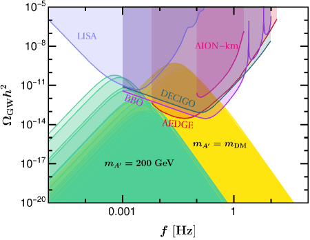
Figure 3: The GW signals induced from the dark phase transition in the minimal boson plasma under the one-temperature treatment. Also shown are the sensitivity curves from space-based interferometers, LISA Caprini:2019egz , BBO Cutler:2005qq , and DECIGO Seto:2001qf , as well as from atomic interferometers, AEDGE AEDGE:2019nxb and AION Badurina:2019hst from km-scale terrestrial detectors.

To obtain the GW curves, we perform a numerical scan of the free parameters $\lambda,g_{X}$ in the following range:

$$\lambda=5\times[10^{-4},10^{-2}]\,,\quad g_{X}=[0.1,1]\,.$$ (60)

The resulting $\Omega_{\rm sw}h^{2}$ is shown in Fig. 3. The shaded yellow region denotes the predicted GW signals under the scan (60), where the DM relic density is matched to the observed value via Eq. (33). The peak frequencies for strong GW signals above $10^{-14}$ are located at $0.01-1$ Hz. In particular, the GW curves have some overlap with the updated LISA sensitivity Caprini:2019egz only for large $g_{X}\sim 1$. This result can also be inferred from the analytic phase transition presented in Appendix A. As indicated by Eq. (55), a large GW amplitude favors a small $\beta/\mathcal{H}$ and a large $\alpha$. From the left panel of Fig. 5, we see that a small $\beta/\mathcal{H}$ and a large $\alpha$ requires a large $g_{X}$. It implies that, when $A^{\prime}_{\mu}$ is the DM with relic density fixed via Eq. (33), the dark vacuum $v_{\phi}$ is at $1-10$ TeV. In general, for a non-supercooled phase transition, we expect a nucleation temperature with the magnitude not far from the dark vacuum $v_{\phi}$. Therefore, a large $\Omega_{\rm sw}h^{2}$ favors $T_{n}>100$ GeV. Then, from Eq. (56), we see that the peak frequency can be at $\mathcal{O}(1)$ mHz if $\beta/\mathcal{H}\lesssim 10$. However, as inferred from the left panel of Fig. 5, $\beta/\mathcal{H}<10$ is hard to obtain, unless $g_{X}\gtrsim 1$. We then conclude that the inferred peak frequency for $g_{X}<1$ is above $\mathcal{O}(1)$ mHz where the updated LISA sensitivity curve allows a GW amplitude as low as $\mathcal{O}(10^{-12})$. Therefore, only for some large $g_{X}$ will the induced GW curves have some overlap with the detectable region from LISA.

It becomes clear that when $m_{A^{\prime}}$ and $g_{X}$ are disentangled by making the dark gauge boson unstable, the induced GW peak frequency can shift towards 1 mHz. Indeed, taking $m_{A^{\prime}}=200$ GeV as an example, we can see from the green region that a relatively light dark gauge boson allows more overlap with the detectable region from LISA.

When $A^{\prime}_{\mu}$ is the DM candidate within the minimal dark boson plasma, the strong first-order phase transition can readily induce GW signals that can be detected by the space-based interferometers DECIGO Seto:2001qf and BBO Cutler:2005qq . Furthermore, some proposed atomic interferometers can also capture the induced GW signals. This is particularly the case for the AION experiment with km-scale terrestrial detectors Badurina:2019hst . The space experiment AEDGE AEDGE:2019nxb that uses cold atoms to search for ultra-light DM and GW is also able to capture the GW induced from the minimal dark bosonic phase transition.

BP	$\lambda$	$g_{X}$	$T_{n}$	$\alpha$	$\beta/\mathcal{H}$
LISA	$1.7\times 10^{-2}$	0.97	2.4 TeV	0.74	45
AION	$3.0\times 10^{-3}$	0.61	0.93 TeV	0.80	417
DECIGO	$8.7\times 10^{-4}$	0.44	0.48 TeV	0.89	1304
BBO	$8.3\times 10^{-4}$	0.43	0.58 TeV	0.30	1561

Table 1: Selected BP for GW signals detectable by LISA, AION, DECIGO and BBO, respectively.

Finally, we would like to comment on the LISA sensitivity curve adopted in this paper. In fact, there are some analyses of difference LISA sensitivity curves used in the literature. In particular, the analysis based on the peak-integrated-sensitivity curves in Ref. Schmitz:2020syl pointed out a lower curve of the LISA sensitivity. In this case, the induced GW signals from the minimal dark boson plasma would have more overlap with the estimated sensitivity region. In this paper, we do not show the peak-integrated-sensitivity curve of LISA, so our conclusions are based on the updated LISA sensitivity from Ref. Caprini:2019egz .

6 Hear and see the dark: complementary tests of DM, GW and colliders

Given the current constraints and the future sensitivities, it is tempting to ask whether the parameter space for a dark first-order phase transition, observable GW signals and DM favors a Higgs portal coupling that can be probed by collider detection. To this end, we select four BP from Fig. 3, which respectively corresponds to a GW curve overlapping with the LISA region (BP for LISA), residing between LISA and AION (BP for AION), between AION and DECIGO (BP for DECIGO), and between DECIGO and BBO (BP for BBO). The parameters for each BP are shown in Tab. 1.

The first thing to notice from these BP is that, the predicted scalar masses are all above $2m_{h}$, so the constraints and future detection from the Higgs invisible decay are not applicable. In fact, a heavy dark scalar is generically expected when $A^{\prime}_{\mu}$ is the DM candidate. As discussed in Sec. 5, $g_{X}>0.1$ and $\lambda>10^{-4}$ are required to induce strong GW signals. Then we can infer from Eq. (33) and Eq. (5) that the dark scalar mass is well above 10 GeV. When $A^{\prime}_{\mu}$ is no longer a stable DM, the dark scalar can be lighter such that the constraints and future detection of the Higgs invisible decay come into play, as discussed in Ref. Li:2023bxy .

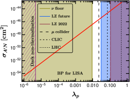
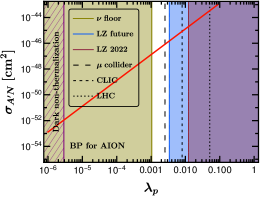
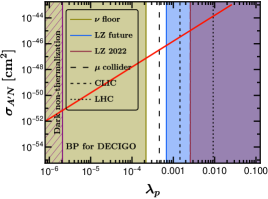
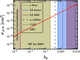
Figure 4: The parameter space for complementary tests from colliders, DM direct detection and GW interferometers. The spin-independent DM-nucleon cross section in terms of the Higgs portal coupling $\lambda_{p}$ is shown for each BP.

For heavy dark scalar above $2m_{h}$, the channel $\text{SM}\to\phi\to\text{SM}$ will serve as the direct collider probe. Currently, the constraints in this channel are set by the LHC with an upper limit of $\theta$ at the level of 0.1. Future sensitivities from 3 TeV CLIC with an integrated luminosity $3\leavevmode\nobreak\ \text{ab}^{-1}$ in the decay channel $\phi\to 2h$ can reach a level of $\sin\theta^{2}\approx 0.001$ Linssen:2012hp ; Buttazzo:2018qqp and the 14 TeV muon collider with an integrated luminosity $14\leavevmode\nobreak\ \text{ab}^{-1}$ can further probe the mixing angle down to $\sin\theta^{2}\approx 10^{-4}$ for $m_{\phi}<3$ TeV Buttazzo:2018qqp . The dashed lines shown in Fig. 4 (from right to left) correspond to the limit of $\theta$ excluded by current LHC, detectable by future CLIC and muon collider, respectively. Note that, the indirect collider probes via the coupling strength modifier $\kappa_{Z}$ will reach a sensitivity of $\theta\simeq 0.06$, e.g., at the ILC, CEPC and FCC-ee, which is comparable with the limit reachable by direct detection from the future 3 TeV CLIC.

We show in Fig. 4 the curve of the predicted spin-independent DM-nucleon cross section in terms of the portal coupling in each BP. The rightmost shaded region in each panel is excluded by the LZ experiment LZ:2022ufs . The middle shaded region corresponds to the future LZ sensitivity LZ:2018qzl . The leftmost shaded region corresponds to the neutrino floor for xenon experiment Ruppin:2014bra , when the direct detection of DM suffers from irreducible background of coherent neutrino-nucleus scattering. We can see that the Higgs portal coupling down to the level of $10^{-3}$ can be probed by the future LZ experiment, and the spin-independent DM-nucleon cross section can reach as large as $\sigma_{A^{\prime}N}\simeq\mathcal{O}(10^{-45})\leavevmode\nobreak\ \text{cm}^{2}$.

Combining the GW signals, DM direct detection and the collider tests, we can see that for all the BP, the CLIC is able to test a portion of the parameter space that induces GW signals observable by LISA, AION, DECIGO and BBO, respectively. For all the panels shown in Fig. 4, we can see that the future muon collider can probe a portal coupling above the neutrino floor for the xenon experiment, and can fully test the parameter space that predicts a spin-independent DM-nucleon cross section within the future LZ sensitivity. We then obtain an interesting situation for the minimal dark boson world: when the stochastic GW signals are observed by future space-based/terrestrial interferometers, complementary probes via direct detection of a vector DM particle and collider searches for a dark scalar singlet can provide cross-checks for the microscopic origin of the GW signals.

Finally, as mentioned in Sec. 2.3, the dark thermalization conditions for the one-temperature treatment of the dark phase transition and DM freeze-out typically require a Higgs portal coupling at $\lambda_{p}>\mathcal{O}(10^{-6})$. This is shown in Fig. 4, where the purple meshed region denotes a small $\lambda_{p}$ that cannot establish a thermal contact between the SM and the dark sectors all the way down to the DM freeze-out temperature $T_{\rm fo}\simeq m_{A^{\prime}}/25$. It points out that, for a Higgs-portal connected minimal dark sector, the interested parameter space for strong GW signals and detectable DM indeed corresponds to a dark boson plasma sharing the same temperature with the SM during the phase transition and the DM freeze-out.

7 Conclusion

We have presented a dark boson plasma that can undergo a strong first-order phase transition, generate observable GW signals and provide a DM candidate. The dark gauge boson, as the WIMP-like DM, plays a significant role in triggering the dark phase transition via finite-temperature effects and hence inducing stochastic GW signals. The theoretical framework is so simple and minimal that certain correlations exist in the complementary tests from GW interferometers, direct detection of DM and colliders, all of which serve as promising avenues to help us hear and see the dark. In particular, we found that the future muon collider in the decay channel $\phi\to 2h$ is able to probe the full parameter space where GW signals induced from the dark phase transition are detectable by LISA, DECIGO, BBO, AION and AEDGE, and the spin-independent DM-nucleon cross section is reachable by the future LZ experiment above the neutrino floor.

Appendix A An analytic perspective of the minimal dark phase transition

An analytic analysis of the dark phase transition allows us to get an efficient overview of the model parameter space where strong GW signals are favored and the connection to DM could become clearer. In this appendix, we discuss the analytic dynamics of the dark phase transition by making some reasonable approximations. We will see that, such an analytic perspective is qualitatively consistent with the numerical analysis performed in the main text.

One of the widely considered potentials that allow analytic treatments Dine:1992wr ; Quiros:1999jp has the following polynomial structure Quiros:1999jp ,

$$V_{\rm poly}(\varphi,T)=D(T^{2}-T_{0}^{2})\varphi^{2}-ET\varphi^{3}+\frac{\lambda}{4}\varphi^{4}\,,$$ (61)

with field-independent constants $D,T_{0},E$. This polynomial potential is also expected from the minimal dark $U(1)_{X}$ scenario considered in this work. Explicitly, it can be derived by using the high-temperature expansion of Eq. (42) Dolan:1973qd ; Laine:2016hma ,

$$V_{T} \approx\frac{T^{2}}{24}\sum_{i=\phi,\chi,A^{\prime}}n_{i}m_{i}^{2}-\frac{T}{12\pi}\sum_{i=\phi,\chi,A^{\prime}}n_{i}(m_{i}^{2})^{3/2}-\frac{1}{64\pi^{2}}\sum_{i=\phi,\chi,A^{\prime}}n_{i}m_{i}^{4}\ln\left(\frac{m_{i}^{2}}{aT^{2}}\right),$$ (62)

where $\ln a\approx 5.41$ and we have dropped the $\varphi$-independent constants.

The $\mu$-dependence from $V_{\rm CW}$ in Eq. (38) can be removed by invoking the RG running of the tree-level parameters in $V_{0}$ Kastening:1991gv ; Bando:1992np ; Ford:1992mv , with

$$\lambda(\mu) =\lambda(\mu_{0})+\frac{3g_{X}^{4}}{16\pi^{2}}\ln\left(\frac{\mu^{2}}{\mu_{0}^{2}}\right)+\mathcal{O}(\lambda^{2})\,,$$ (63)

$$\mu_{S}^{2}(\mu) =\mu_{S}^{2}(\mu_{0})+\frac{\lambda(\mu_{0})}{4\pi^{2}}\mu_{S}^{2}(\mu_{0})\ln\left(\frac{\mu^{2}}{\mu_{0}^{2}}\right).$$ (64)

After applying the daisy resummation (44), we finally arrive at the effective potential

$$V_{{\rm eff}}(\varphi,T)=\left(\frac{g_{X}^{2}}{8}T^{2}-\frac{\lambda v^{2}_{\phi}}{2}\right)\varphi^{2}-\frac{g_{X}^{3}T}{12\pi}\left[2\varphi^{3}+\left(\varphi^{2}+\frac{T^{2}}{3}\right)^{3/2}\right]+\frac{\lambda}{4}\varphi^{4}\,,$$ (65)

where only the dominant contribution from the gauge boson is taken into account, and corrections at $\mathcal{O}(\lambda^{2})$ and terms proportional to $3g_{X}^{4}/(4\pi)^{2}$ in Eqs. (63) and (64) are neglected.

It can now be seen that, without the daisy resummation in Eq. (65), the effective potential reduces to the polynomial form (61), with

$$D=\frac{g_{X}^{2}}{8}\,,\quad T_{0}=\frac{2\sqrt{\lambda}v_{\phi}}{g_{X}}\,,\quad E=\frac{g_{X}^{2}}{4\pi}\,.$$ (66)

The potential (61) at high temperatures could develop an energy barrier between the false and true vacua. As usual, there is a trivial solution ${\varphi}=0$ to $\partial{V}_{\rm poly}/\partial{\varphi}=0$, corresponding to a local minimum if $4\lambda v_{\phi}^{2}<g_{X}^{2}{T}^{2}$. There are two additional solutions to $\partial{V}_{\rm poly}/\partial{\varphi}=0$, with

$${\varphi}_{\pm}=\frac{1}{8\pi\lambda}\left[3g_{X}^{3}T\pm(9g_{X}^{6}{T}^{2}-16\pi^{2}g_{X}^{2}\lambda{T}^{2}+64\pi^{2}\lambda^{2}v_{\phi}^{2})^{1/2}\right].$$ (67)

To make these extrema physical, we should set

$$64\pi^{2}\lambda^{2}v_{\phi}^{2}-16\pi^{2}g_{X}^{2}\lambda T^{2}+9g_{X}^{6}T^{2}>0\,,$$ (68)

for temperatures $T$ during the phase transition. The local maximum at ${\varphi}_{-}$ is expected to develop an energy barrier between the false vacuum at ${\varphi}=0$ and the true vacuum at ${\varphi}_{+}$.

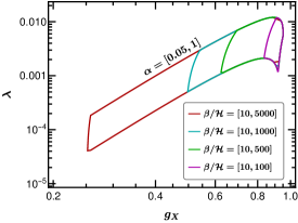
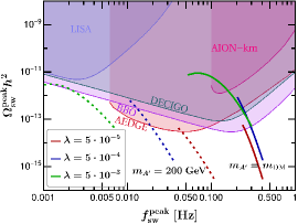
Figure 5: Left: the parameter space in terms of $\lambda$ and $g_{X}$ for $0.05<\alpha<1$ and for some typical ranges of $\beta/\mathcal{H}$. Right: the correlation between the GW peak amplitude $\Omega_{\rm sw}^{\rm peak}h^{2}$ and peak frequency $f_{\rm sw}^{\rm peak}$ for some benchmark values of $\lambda$ under the scan of $0.1<g_{X}<1$. The solid lines are obtained via Eq. (33) while the dotted lines are obtained by fixing $m_{A^{\prime}}=200$ GeV without assuming a DM candidate.

The Euclidean action $S_{3}$ from the polynomial potential has the following simple analytic solution Adams:1993zs ,

$$S_{3}\approx\frac{64\pi ET\sqrt{\delta}(\beta_{1}\delta+\beta_{2}\delta^{2}+\beta_{3}\delta^{3})}{81\lambda^{3/2}(2-\delta)^{2}}\,,$$ (69)

where $\delta\equiv 2\lambda D(1-T_{0}^{2}/T^{2})/E^{2}$, with $D,T_{0}$ and $E$ given in Eq. (66), and $\beta_{1}=8.2938,\beta_{2}=-5.5330,\beta_{3}=0.8180$. Using this analytic expression, we can evaluate the nucleation temperature via Eq. (49), and subsequently the $\alpha,\beta/\mathcal{H}$ parameters.

We show in the left panel of Fig. 5 the parameter space of $\lambda,g_{X}$ for $0.05<\alpha<1$ and some typical ranges of $\beta/\mathcal{H}$. By taking some BP of $\lambda$ inferred from the left panel, we scan the gauge coupling in the range: $[0.1,1]$, so as to obtain the relation between $f_{\rm sw}^{\rm peak}$ and $\Omega_{\rm sw}^{\rm peak}h^{2}$ from Eqs. (55) and (56), as shown in the right panel of Fig. 5. Both the short solid and dotted lines are cut by the conditions $0.1<\alpha<1,\beta/\mathcal{H}>1$ and (68).

It can be seen that, when $A^{\prime}_{\mu}$ is the DM candidate, the condition from Eq. (33) implies a peak frequency at sub-Hz, with the peak amplitude detectable by AION, AEDGE, DECIGO and BBO. When relaxing the DM condition, we take a lower mass for the dark gauge boson, $m_{A^{\prime}}=200$ GeV, which shifts the peak frequency towards mHz. Note that the LISA sensitivity curve is taken from the analysis given in Ref. Caprini:2019egz , rather than the peak-integrated-sensitivity curves from Refs. Alanne:2019bsm ; Schmitz:2020syl .

Appendix B DM annihilation rates

The gauge-scalar interaction is derived from the gauge kinetic term:

$$\mathcal{L}_{\rm kin}=(\partial_{\mu}-ig_{X}A^{\prime}_{\mu})S\cdot(\partial^{\mu}+ig_{X}A^{\prime\mu})S^{*},$$ (70)

with $S=(v_{\phi}+\phi)/\sqrt{2}$ in the unitary gauge. It leads to the vertices,

$$A^{\prime\mu}A^{\prime\nu}\phi :2g_{X}^{2}v_{\phi}\eta^{\mu\nu}\,,\qquad A^{\prime\mu}A^{\prime\nu}\phi^{2}:2g_{X}^{2}\eta^{\mu\nu}\,,$$ (71)

where $\eta^{\mu\nu}$ is the Minkowski metric. For the dark scalar $\phi$, the Feynman vertices from potential (1) are given by

$$\phi^{3} :-6\lambda v_{\phi}\,,\qquad\phi^{4}:-6\lambda\,.$$ (72)

The dark gauge boson freeze-out is dominated by the quartic contact interaction and the $t,u$-channel annihilation, while the $s$-channel annihilation carries an additional factor $\lambda^{2}$ and hence is much smaller than the $t,u$ channels for $\lambda\ll g_{X}^{2}$. Neglecting the $s$-channel is a good approximation since there is no $s$-channel resonant production of $\phi$ for $m_{A^{\prime}}\gg m_{\phi}$. The cross section of $2A^{\prime}_{\mu}\to 2\phi$ can be parameterized as

$$\sigma v \equiv 2(a+bv^{2})\,,$$ (73)

where the factor of 2 takes into account the pair DM annihilation, and $v$ is the relative velocity of incoming DM particles. To determine the cross section, let us now calculate the amplitude of $2A^{\prime}_{\mu}\to 2\phi$, with the Feynman diagrams shown in Fig. 1. The amplitudes in the center-of-mass frame are given by

$$\mathcal{M}_{t} =\frac{8g_{X}^{4}v_{\phi}^{2}\eta^{\mu\nu}\epsilon_{\mu}(p_{1})\epsilon_{\nu}(p_{2})}{m_{\phi}^{2}-\hat{s}(1-\beta_{A^{\prime}}\beta_{\phi}\cos\theta)}\,,$$ (74)

$$\mathcal{M}_{u} =\frac{8g_{X}^{4}v_{\phi}^{2}\eta^{\mu\nu}\epsilon_{\mu}(p_{1})\epsilon_{\nu}(p_{2})}{m_{\phi}^{2}-\hat{s}(1+\beta_{A^{\prime}}\beta_{\phi}\cos\theta)}\,,$$ (75)

$$\mathcal{M}_{c} =2g_{X}^{2}\eta^{\mu\nu}\epsilon_{\mu}(p_{1})\epsilon_{\nu}(p_{2})\,,$$ (76)

for the $t,u$ channels and contact annihilation, respectively. Here $\hat{s}$ is the Lotentz-invariant Mandelstam variable, $\beta_{A^{\prime},\phi}\equiv\sqrt{1-4m_{A^{\prime},\phi}^{2}/\hat{s}}$, and $\theta$ is the angle between the momenta of the incoming and outgoing particles in the center-of-mass frame.

The differential cross section in the center-of-mass frame yields

$$\frac{d\sigma}{d\Omega}=\frac{1}{S(2E_{1})(2E_{2})|\vec{v}_{1}-\vec{v}_{2}|}\left[\frac{1}{16\pi^{2}}\frac{|\vec{p}_{f}|}{E_{{\rm cm}}}|\mathcal{M}|^{2}_{\rm sum}\right]=\frac{\beta_{\phi}|\mathcal{M}|^{2}_{\rm sum}}{128\pi^{2}\beta_{A^{\prime}}\hat{s}}\,,$$ (77)

where $\mathcal{M}_{\rm sum}=\mathcal{M}_{t}+\mathcal{M}_{u}+\mathcal{M}_{c}$, $1/S=1/2$ is the symmetry factor accounting for the identical scalar in the final states, and $E_{\rm cm}=\sqrt{\hat{s}}$. The final-state momentum $|\vec{p}_{f}|$ in the center-of-mass frame can be expressed in terms of $\hat{s}$, with $|\vec{p}_{f}|=\beta_{\phi}\sqrt{\hat{s}}/2$.

Going to the frame where one of the incoming particles is at rest, as defined in Eq. (73), we can parameterize the incoming four-momenta as $p_{1}=(E,\vec{p}),p_{2}=(m_{A^{\prime}},0)$, with the relative velocity $v=|\vec{p}/E|$. Given $E=m_{A^{\prime}}/\sqrt{1-v^{2}},|\vec{p}|=m_{A^{\prime}}v/\sqrt{{1-v^{2}}}$, $\hat{s}$ in the relative frame is given by

$$\hat{s}=(p_{1}+p_{2})^{2}=2m_{A^{\prime}}^{2}(1+\frac{1}{\sqrt{1-v^{2}}})\approx 4m_{A^{\prime}}^{2}(1+v^{2}/4)\,.$$ (78)

It is now straightforward to evaluate the cross section in the relative frame. Expanding the small velocity up to $\mathcal{O}(v^{2})$ and neglecting the scalar mass, we obtain the $a,b$ parameters as

$$a\approx\frac{3g_{X}^{4}}{16\pi m_{A^{\prime}}^{2}}\,,\quad b\approx-\frac{15g_{X}^{4}}{128\pi m_{A^{\prime}}^{2}}\,.$$ (79)

Based on Eq. (73), the collision rate $\gamma_{A^{\prime}}$ can be written as

$$\gamma_{A^{\prime}} =\int d\Pi_{1}d\Pi_{2}d\Pi_{3}d\Pi_{4}f_{1}(E_{1})f_{2}(E_{2})|\mathcal{M}|_{\rm sum}^{2}(2\pi)^{4}\delta^{4}\left(p_{1}+p_{2}-p_{3}-p_{4}\right)$$ (80)

$$=\int d\Pi_{1}d\Pi_{2}f_{1}(E_{1})f_{2}(E_{2})[4\sigma vE_{1}E_{2}]$$ (81)

$$=2(a+3b/x)n_{A^{\prime}}^{2}$$ (82)

$$\equiv\langle\sigma v\rangle_{A^{\prime}}n_{A^{\prime}}^{2}\,,$$ (83)

where $d\Pi_{i}\equiv d^{3}p_{i}/[(2\pi)^{3}2E_{i}]$ is the phase-space factor with $E_{i}$ the energy, $f_{i}(E_{i})$ is the thermal distribution function of $A^{\prime}_{\mu}$ with the number density $n_{A^{\prime}}$, and the quantum statistics for the final states is neglected. Note that in Eq. (82), $x\equiv m_{A^{\prime}}/T$, and the $b$-dependent term is derived by taking the relative velocity $v^{2}=p_{1}^{2}/E_{1}^{2}\approx p_{1}^{2}/m_{A^{\prime}}^{2}$ in the phase-space integration with the Boltzmann distribution $f_{1}(E_{1})=e^{-E_{1}/T}$, since the DM freeze-out occurs when $A^{\prime}_{\mu}$ becomes nonrelativistic.

References

- (1) P. Schwaller, Gravitational Waves from a Dark Phase Transition, Phys. Rev. Lett. 115 (2015), no. 18 181101, [1504.07263].
- (2) M. Pospelov, A. Ritz, and M. B. Voloshin, Secluded WIMP Dark Matter, Phys. Lett. B 662 (2008) 53–61, [0711.4866].
- (3) J. L. Feng, H. Tu, and H.-B. Yu, Thermal Relics in Hidden Sectors, JCAP 10 (2008) 043, [0808.2318].
- (4) A. Berlin, D. Hooper, and G. Krnjaic, Thermal Dark Matter From A Highly Decoupled Sector, Phys. Rev. D 94 (2016), no. 9 095019, [1609.02555].
- (5) J. A. Evans, S. Gori, and J. Shelton, Looking for the WIMP Next Door, JHEP 02 (2018) 100, [1712.03974].
- (6) B. Batell, N. Blinov, C. Hearty, and R. McGehee, Exploring Dark Sector Portals with High Intensity Experiments, in Snowmass 2021, 7, 2022. 2207.06905.
- (7) T. Ferber, A. Grohsjean, and F. Kahlhoefer, Dark Higgs Bosons at Colliders, 2305.16169.
- (8) J. Jaeckel, V. V. Khoze, and M. Spannowsky, Hearing the signal of dark sectors with gravitational wave detectors, Phys. Rev. D 94 (2016), no. 10 103519, [1602.03901].
- (9) R. Jinno and M. Takimoto, Probing a classically conformal B-L model with gravitational waves, Phys. Rev. D 95 (2017), no. 1 015020, [1604.05035].
- (10) C.-W. Chiang and E. Senaha, On gauge dependence of gravitational waves from a first-order phase transition in classical scale-invariant models, Phys. Lett. B 774 (2017) 489–493, [1707.06765].
- (11) V. Brdar, A. J. Helmboldt, and J. Kubo, Gravitational Waves from First-Order Phase Transitions: LIGO as a Window to Unexplored Seesaw Scales, JCAP 02 (2019) 021, [1810.12306].
- (12) C. Marzo, L. Marzola, and V. Vaskonen, Phase transition and vacuum stability in the classically conformal B–L model, Eur. Phys. J. C 79 (2019), no. 7 601, [1811.11169].
- (13) S. Yaser Ayazi and A. Mohamadnejad, Conformal vector dark matter and strongly first-order electroweak phase transition, JHEP 03 (2019) 181, [1901.04168].
- (14) A. Mohamadnejad, Gravitational waves from scale-invariant vector dark matter model: Probing below the neutrino-floor, Eur. Phys. J. C 80 (2020), no. 3 197, [1907.08899].
- (15) J. Ellis, M. Lewicki, J. M. No, and V. Vaskonen, Gravitational wave energy budget in strongly supercooled phase transitions, JCAP 06 (2019) 024, [1903.09642].
- (16) J. Ellis, M. Lewicki, and V. Vaskonen, Updated predictions for gravitational waves produced in a strongly supercooled phase transition, JCAP 11 (2020) 020, [2007.15586].
- (17) A. Addazi and A. Marciano, Gravitational waves from dark first order phase transitions and dark photons, Chin. Phys. C 42 (2018), no. 2 023107, [1703.03248].
- (18) D. Croon, V. Sanz, and G. White, Model Discrimination in Gravitational Wave spectra from Dark Phase Transitions, JHEP 08 (2018) 203, [1806.02332].
- (19) M. Breitbach, J. Kopp, E. Madge, T. Opferkuch, and P. Schwaller, Dark, Cold, and Noisy: Constraining Secluded Hidden Sectors with Gravitational Waves, JCAP 07 (2019) 007, [1811.11175].
- (20) T. Hasegawa, N. Okada, and O. Seto, Gravitational waves from the minimal gauged model, Phys. Rev. D 99 (2019), no. 9 095039, [1904.03020].
- (21) J. B. Dent, B. Dutta, S. Ghosh, J. Kumar, and J. Runburg, Sensitivity to dark sector scales from gravitational wave signatures, JHEP 08 (2022) 300, [2203.11736].
- (22) S.-P. Li and K.-P. Xie, A collider test of nano-Hertz gravitational waves from pulsar timing arrays, 2307.01086.
- (23) I. Baldes, Gravitational waves from the asymmetric-dark-matter generating phase transition, JCAP 05 (2017) 028, [1702.02117].
- (24) F. P. Huang and C. S. Li, Probing the baryogenesis and dark matter relaxed in phase transition by gravitational waves and colliders, Phys. Rev. D 96 (2017), no. 9 095028, [1709.09691].
- (25) L. Bian and Y.-L. Tang, Thermally modified sterile neutrino portal dark matter and gravitational waves from phase transition: The Freeze-in case, JHEP 12 (2018) 006, [1810.03172].
- (26) I. Baldes and C. Garcia-Cely, Strong gravitational radiation from a simple dark matter model, JHEP 05 (2019) 190, [1809.01198].
- (27) M. Kierkla, A. Karam, and B. Swiezewska, Conformal model for gravitational waves and dark matter: a status update, JHEP 03 (2023) 007, [2210.07075].
- (28) S. R. Coleman and E. J. Weinberg, Radiative Corrections as the Origin of Spontaneous Symmetry Breaking, Phys. Rev. D 7 (1973) 1888–1910.
- (29) High-Luminosity Large Hadron Collider (HL-LHC): Technical Design Report V. 0.1, .
- (30) Physics and Detectors at CLIC: CLIC Conceptual Design Report, 1202.5940.
- (31) ILC Collaboration, The International Linear Collider Technical Design Report - Volume 2: Physics, 1306.6352.
- (32) J. P. Delahaye, M. Diemoz, K. Long, B. Mansoulié, N. Pastrone, L. Rivkin, D. Schulte, A. Skrinsky, and A. Wulzer, Muon Colliders, 1901.06150.
- (33) LUX Collaboration, D. S. Akerib et al., Results from a search for dark matter in the complete LUX exposure, Phys. Rev. Lett. 118 (2017), no. 2 021303, [1608.07648].
- (34) XENON Collaboration, E. Aprile et al., First Dark Matter Search Results from the XENON1T Experiment, Phys. Rev. Lett. 119 (2017), no. 18 181301, [1705.06655].
- (35) PandaX-II Collaboration, X. Cui et al., Dark Matter Results From 54-Ton-Day Exposure of PandaX-II Experiment, Phys. Rev. Lett. 119 (2017), no. 18 181302, [1708.06917].
- (36) PandaX-4T Collaboration, Y. Meng et al., Dark Matter Search Results from the PandaX-4T Commissioning Run, Phys. Rev. Lett. 127 (2021), no. 26 261802, [2107.13438].
- (37) LZ Collaboration, J. Aalbers et al., First Dark Matter Search Results from the LUX-ZEPLIN (LZ) Experiment, 2207.03764.
- (38) C. Caprini et al., Detecting gravitational waves from cosmological phase transitions with LISA: an update, JCAP 03 (2020) 024, [1910.13125].
- (39) C. Cutler and J. Harms, BBO and the neutron-star-binary subtraction problem, Phys. Rev. D 73 (2006) 042001, [gr-qc/0511092].
- (40) N. Seto, S. Kawamura, and T. Nakamura, Possibility of direct measurement of the acceleration of the universe using 0.1-Hz band laser interferometer gravitational wave antenna in space, Phys. Rev. Lett. 87 (2001) 221103, [astro-ph/0108011].
- (41) L. Badurina et al., AION: An Atom Interferometer Observatory and Network, JCAP 05 (2020) 011, [1911.11755].
- (42) AEDGE Collaboration, Y. A. El-Neaj et al., AEDGE: Atomic Experiment for Dark Matter and Gravity Exploration in Space, EPJ Quant. Technol. 7 (2020) 6, [1908.00802].
- (43) LZ Collaboration, D. S. Akerib et al., LUX-ZEPLIN (LZ) Conceptual Design Report, 1509.02910.
- (44) B. J. Mount et al., LUX-ZEPLIN (LZ) Technical Design Report, 1703.09144.
- (45) LZ Collaboration, D. S. Akerib et al., Projected WIMP sensitivity of the LUX-ZEPLIN dark matter experiment, Phys. Rev. D 101 (2020), no. 5 052002, [1802.06039].
- (46) J. Billard, L. Strigari, and E. Figueroa-Feliciano, Implication of neutrino backgrounds on the reach of next generation dark matter direct detection experiments, Phys. Rev. D 89 (2014), no. 2 023524, [1307.5458].
- (47) F. Ruppin, J. Billard, E. Figueroa-Feliciano, and L. Strigari, Complementarity of dark matter detectors in light of the neutrino background, Phys. Rev. D 90 (2014), no. 8 083510, [1408.3581].
- (48) O. Lebedev, H. M. Lee, and Y. Mambrini, Vector Higgs-portal dark matter and the invisible Higgs, Phys. Lett. B 707 (2012) 570–576, [1111.4482].
- (49) Y. Farzan and A. R. Akbarieh, VDM: A model for Vector Dark Matter, JCAP 10 (2012) 026, [1207.4272].
- (50) V. Vaskonen, Electroweak baryogenesis and gravitational waves from a real scalar singlet, Phys. Rev. D 95 (2017), no. 12 123515, [1611.02073].
- (51) A. Beniwal, M. Lewicki, J. D. Wells, M. White, and A. G. Williams, Gravitational wave, collider and dark matter signals from a scalar singlet electroweak baryogenesis, JHEP 08 (2017) 108, [1702.06124].
- (52) K. Hashino, M. Kakizaki, S. Kanemura, P. Ko, and T. Matsui, Gravitational waves from first order electroweak phase transition in models with the U(1)X gauge symmetry, JHEP 06 (2018) 088, [1802.02947].
- (53) A. Denner, S. Heinemeyer, I. Puljak, D. Rebuzzi, and M. Spira, Standard Model Higgs-Boson Branching Ratios with Uncertainties, Eur. Phys. J. C 71 (2011) 1753, [1107.5909].
- (54) CMS Collaboration, A. M. Sirunyan et al., Search for invisible decays of a Higgs boson produced through vector boson fusion in proton-proton collisions at 13 TeV, Phys. Lett. B 793 (2019) 520–551, [1809.05937].
- (55) J. de Blas et al., Higgs Boson Studies at Future Particle Colliders, JHEP 01 (2020) 139, [1905.03764].
- (56) Y. Tan et al., Search for invisible decays of the Higgs boson produced at the CEPC, Chin. Phys. C 44 (2020), no. 12 123001, [2001.05912].
- (57) A. Ishikawa, Search for invisible decays of the Higgs boson at the ILC, PoS LeptonPhoton2019 (2019) 147, [1909.07537].
- (58) K. Fujii et al., ILC Study Questions for Snowmass 2021, 2007.03650.
- (59) C. Potter, A. Steinhebel, J. Brau, A. Pryor, and A. White, Expected Sensitivity to Invisible Higgs Boson Decays at the ILC with the SiD Detector, 2203.08330.
- (60) CMS Collaboration, A. M. Sirunyan et al., Search for a new scalar resonance decaying to a pair of Z bosons in proton-proton collisions at TeV, JHEP 06 (2018) 127, [1804.01939]. [Erratum: JHEP 03, 128 (2019)].
- (61) CMS Collaboration, A. Tumasyan et al., Search for a heavy Higgs boson decaying into two lighter Higgs bosons in the bb final state at 13 TeV, JHEP 11 (2021) 057, [2106.10361].
- (62) ATLAS Collaboration, M. Aaboud et al., Combination of searches for heavy resonances decaying into bosonic and leptonic final states using 36 fb-1 of proton-proton collision data at TeV with the ATLAS detector, Phys. Rev. D 98 (2018), no. 5 052008, [1808.02380].
- (63) ATLAS Collaboration, G. Aad et al., Search for heavy diboson resonances in semileptonic final states in pp collisions at TeV with the ATLAS detector, Eur. Phys. J. C 80 (2020), no. 12 1165, [2004.14636].
- (64) ATLAS Collaboration, G. Aad et al., Search for heavy resonances decaying into a pair of Z bosons in the and final states using 139 of proton–proton collisions at TeV with the ATLAS detector, Eur. Phys. J. C 81 (2021), no. 4 332, [2009.14791].
- (65) ATLAS Collaboration, G. Aad et al., Search for resonant and non-resonant Higgs boson pair production in the decay channel using 13 TeV pp collision data from the ATLAS detector, JHEP 07 (2023) 040, [2209.10910].
- (66) D. Buttazzo, D. Redigolo, F. Sala, and A. Tesi, Fusing Vectors into Scalars at High Energy Lepton Colliders, JHEP 11 (2018) 144, [1807.04743].
- (67) LHC Higgs Cross Section Working Group Collaboration, J. R. Andersen et al., Handbook of LHC Higgs Cross Sections: 3. Higgs Properties, 1307.1347.
- (68) ATLAS Collaboration, A detailed map of Higgs boson interactions by the ATLAS experiment ten years after the discovery, Nature 607 (2022), no. 7917 52–59, [2207.00092]. [Erratum: Nature 612, E24 (2022)].
- (69) CMS Collaboration, A. Tumasyan et al., A portrait of the Higgs boson by the CMS experiment ten years after the discovery, Nature 607 (2022), no. 7917 60–68, [2207.00043].
- (70) R. K. Ellis et al., Physics Briefing Book: Input for the European Strategy for Particle Physics Update 2020, 1910.11775.
- (71) G. C. Branco, P. M. Ferreira, L. Lavoura, M. N. Rebelo, M. Sher, and J. P. Silva, Theory and phenomenology of two-Higgs-doublet models, Phys. Rept. 516 (2012) 1–102, [1106.0034].
- (72) S. Kanemura, K. Tsumura, K. Yagyu, and H. Yokoya, Fingerprinting nonminimal Higgs sectors, Phys. Rev. D 90 (2014) 075001, [1406.3294].
- (73) P. Gondolo and G. Gelmini, Cosmic abundances of stable particles: Improved analysis, Nucl. Phys. B 360 (1991) 145–179.
- (74) J. M. Cline, K. Kainulainen, and K. A. Olive, Protecting the primordial baryon asymmetry from erasure by sphalerons, Phys. Rev. D 49 (1994) 6394–6409, [hep-ph/9401208].
- (75) S. Kanemura, S. Matsumoto, T. Nabeshima, and N. Okada, Can WIMP Dark Matter overcome the Nightmare Scenario?, Phys. Rev. D 82 (2010) 055026, [1005.5651].
- (76) S. Baek, P. Ko, W.-I. Park, and E. Senaha, Higgs Portal Vector Dark Matter : Revisited, JHEP 05 (2013) 036, [1212.2131].
- (77) E. W. Kolb and M. S. Turner, The Early Universe, vol. 69. 1990.
- (78) Particle Data Group Collaboration, R. L. Workman et al., Review of Particle Physics, PTEP 2022 (2022) 083C01.
- (79) Planck Collaboration, N. Aghanim et al., Planck 2018 results. VI. Cosmological parameters, Astron. Astrophys. 641 (2020) A6, [1807.06209]. [Erratum: Astron.Astrophys. 652, C4 (2021)].
- (80) K. Griest and M. Kamionkowski, Unitarity Limits on the Mass and Radius of Dark Matter Particles, Phys. Rev. Lett. 64 (1990) 615.
- (81) B. W. Lee, C. Quigg, and H. B. Thacker, Weak Interactions at Very High-Energies: The Role of the Higgs Boson Mass, Phys. Rev. D 16 (1977) 1519.
- (82) DARWIN Consortium Collaboration, L. Baudis, DARWIN: dark matter WIMP search with noble liquids, J. Phys. Conf. Ser. 375 (2012) 012028, [1201.2402].
- (83) M. Schumann, L. Baudis, L. Bütikofer, A. Kish, and M. Selvi, Dark matter sensitivity of multi-ton liquid xenon detectors, JCAP 10 (2015) 016, [1506.08309].
- (84) J. D. Lewin and P. F. Smith, Review of mathematics, numerical factors, and corrections for dark matter experiments based on elastic nuclear recoil, Astropart. Phys. 6 (1996) 87–112.
- (85) R. J. Hill and M. P. Solon, Standard Model anatomy of WIMP dark matter direct detection II: QCD analysis and hadronic matrix elements, Phys. Rev. D 91 (2015) 043505, [1409.8290].
- (86) M. Hoferichter, P. Klos, J. Menéndez, and A. Schwenk, Improved limits for Higgs-portal dark matter from LHC searches, Phys. Rev. Lett. 119 (2017), no. 18 181803, [1708.02245].
- (87) J. M. Cline and P.-A. Lemieux, Electroweak phase transition in two Higgs doublet models, Phys. Rev. D 55 (1997) 3873–3881, [hep-ph/9609240].
- (88) J. Elias-Miro, J. R. Espinosa, and T. Konstandin, Taming Infrared Divergences in the Effective Potential, JHEP 08 (2014) 034, [1406.2652].
- (89) S. P. Martin, Taming the Goldstone contributions to the effective potential, Phys. Rev. D 90 (2014), no. 1 016013, [1406.2355].
- (90) J. R. Espinosa, T. Konstandin, and F. Riva, Strong Electroweak Phase Transitions in the Standard Model with a Singlet, Nucl. Phys. B 854 (2012) 592–630, [1107.5441].
- (91) P. B. Arnold and O. Espinosa, The Effective potential and first order phase transitions: Beyond leading-order, Phys. Rev. D 47 (1993) 3546, [hep-ph/9212235]. [Erratum: Phys.Rev.D 50, 6662 (1994)].
- (92) A. D. Linde, Fate of the False Vacuum at Finite Temperature: Theory and Applications, Phys. Lett. B 100 (1981) 37–40.
- (93) A. D. Linde, Decay of the False Vacuum at Finite Temperature, Nucl. Phys. B 216 (1983) 421. [Erratum: Nucl.Phys.B 223, 544 (1983)].
- (94) C. L. Wainwright, CosmoTransitions: Computing Cosmological Phase Transition Temperatures and Bubble Profiles with Multiple Fields, Comput. Phys. Commun. 183 (2012) 2006–2013, [1109.4189].
- (95) M. Hindmarsh, S. J. Huber, K. Rummukainen, and D. J. Weir, Numerical simulations of acoustically generated gravitational waves at a first order phase transition, Phys. Rev. D 92 (2015), no. 12 123009, [1504.03291].
- (96) J. R. Espinosa, T. Konstandin, J. M. No, and G. Servant, Energy Budget of Cosmological First-order Phase Transitions, JCAP 06 (2010) 028, [1004.4187].
- (97) S. Höche, J. Kozaczuk, A. J. Long, J. Turner, and Y. Wang, Towards an all-orders calculation of the electroweak bubble wall velocity, JCAP 03 (2021) 009, [2007.10343].
- (98) T. Alanne, T. Hugle, M. Platscher, and K. Schmitz, A fresh look at the gravitational-wave signal from cosmological phase transitions, JHEP 03 (2020) 004, [1909.11356].
- (99) K. Schmitz, New Sensitivity Curves for Gravitational-Wave Signals from Cosmological Phase Transitions, JHEP 01 (2021) 097, [2002.04615].
- (100) C. Caprini et al., Science with the space-based interferometer eLISA. II: Gravitational waves from cosmological phase transitions, JCAP 04 (2016) 001, [1512.06239].
- (101) C. Caprini, R. Durrer, and G. Servant, The stochastic gravitational wave background from turbulence and magnetic fields generated by a first-order phase transition, JCAP 12 (2009) 024, [0909.0622].
- (102) J. Ellis, M. Lewicki, and J. M. No, On the Maximal Strength of a First-Order Electroweak Phase Transition and its Gravitational Wave Signal, JCAP 04 (2019) 003, [1809.08242].
- (103) H.-K. Guo, K. Sinha, D. Vagie, and G. White, Phase Transitions in an Expanding Universe: Stochastic Gravitational Waves in Standard and Non-Standard Histories, JCAP 01 (2021) 001, [2007.08537].
- (104) J. Ellis, M. Lewicki, and J. M. No, Gravitational waves from first-order cosmological phase transitions: lifetime of the sound wave source, JCAP 07 (2020) 050, [2003.07360].
- (105) C. Caprini, D. G. Figueroa, R. Flauger, G. Nardini, M. Peloso, M. Pieroni, A. Ricciardone, and G. Tasinato, Reconstructing the spectral shape of a stochastic gravitational wave background with LISA, JCAP 11 (2019) 017, [1906.09244].
- (106) M. Hindmarsh, S. J. Huber, K. Rummukainen, and D. J. Weir, Shape of the acoustic gravitational wave power spectrum from a first order phase transition, Phys. Rev. D 96 (2017), no. 10 103520, [1704.05871]. [Erratum: Phys.Rev.D 101, 089902 (2020)].
- (107) J. Liu, L. Bian, R.-G. Cai, Z.-K. Guo, and S.-J. Wang, Primordial black hole production during first-order phase transitions, Phys. Rev. D 105 (2022), no. 2 L021303, [2106.05637].
- (108) K. Hashino, S. Kanemura, T. Takahashi, and M. Tanaka, Probing first-order electroweak phase transition via primordial black holes in the effective field theory, Phys. Lett. B 838 (2023) 137688, [2211.16225].
- (109) (XENON Collaboration)††, XENON Collaboration, E. Aprile et al., First Dark Matter Search with Nuclear Recoils from the XENONnT Experiment, Phys. Rev. Lett. 131 (2023), no. 4 041003, [2303.14729].
- (110) M. Dine, R. G. Leigh, P. Y. Huet, A. D. Linde, and D. A. Linde, Towards the theory of the electroweak phase transition, Phys. Rev. D 46 (1992) 550–571, [hep-ph/9203203].
- (111) M. Quiros, Finite temperature field theory and phase transitions, in ICTP Summer School in High-Energy Physics and Cosmology, pp. 187–259, 1, 1999. hep-ph/9901312.
- (112) L. Dolan and R. Jackiw, Symmetry Behavior at Finite Temperature, Phys. Rev. D 9 (1974) 3320–3341.
- (113) M. Laine and A. Vuorinen, Basics of Thermal Field Theory, vol. 925. Springer, 2016.
- (114) B. M. Kastening, Renormalization group improvement of the effective potential in massive phi**4 theory, Phys. Lett. B 283 (1992) 287–292.
- (115) M. Bando, T. Kugo, N. Maekawa, and H. Nakano, Improving the effective potential, Phys. Lett. B 301 (1993) 83–89, [hep-ph/9210228].
- (116) C. Ford, D. R. T. Jones, P. W. Stephenson, and M. B. Einhorn, The Effective potential and the renormalization group, Nucl. Phys. B 395 (1993) 17–34, [hep-lat/9210033].
- (117) F. C. Adams, General solutions for tunneling of scalar fields with quartic potentials, Phys. Rev. D 48 (1993) 2800–2805, [hep-ph/9302321].