Downlink and Uplink NOMA-ISAC
with Signal Alignment

Abstract

Integrated Sensing and Communications (ISAC) surpasses the conventional frequency-division sensing and communications (FDSAC) in terms of spectrum, energy, and hardware efficiency, with potential for greater enhancement through integration of NOMA and signal alignment techniques. Leveraging these advantages, this paper proposes a multiple-input multiple-output NOMA-ISAC framework with signal alignment and thoroughly analyzes its performance for both downlink and uplink. 1) The downlink ISAC is investigated under three different precoding designs: sensing-centric (S-C) design, communications-centric (C-C) design, and Pareto optimal design. 2) For the uplink case, two scenarios are investigated: S-C design and C-C design, based on the interference cancellation order of the communication signal and the sensing signal. In each of these scenarios, key performance metrics including sensing rate (SR), communication rate (CR), and outage probability are investigated. For a deeper understanding, the asymptotic performance of the system in the high signal-to-noise ratio (SNR) region is also explored, with a focus on the high-SNR slope and diversity order. Finally, the SR-CR rate regions achieved by ISAC and FDSAC are studied. Numerical results reveal that in both downlink and uplink cases, ISAC outperforms FDSAC in terms of sensing and communications performance and is capable of achieving a broader rate region, clearly showcasing its superiority over the conventional FDSAC.

I Introduction

The concept of Integrated Sensing and Communications (ISAC) has sparked considerable attention from both the research community and industry due to its immense potential in facilitating the advancement of sixth-generation (6G) and forthcoming wireless networks [1]. A salient attribute of ISAC is its capacity to concurrently utilize the same time, frequency, power, and hardware resources for both communication and sensing purposes. This stands in stark contrast to the conventional approach of Frequency-Division Sensing and Communications (FDSAC), which necessitates distinct frequency bands and infrastructure for the two functions. The efficiency of ISAC is thus expected to surpass FDSAC in terms of spectrum utilization, energy consumption, and hardware requirements [2, 3].

In the assessment of ISAC’s effectiveness, two crucial performance metrics are commonly employed from an information-theoretic standpoint: sensing rate (SR) and communication rate (CR) [3, 4, 5]. The SR is a measure of the system’s capability to accurately estimate environmental information through sensing processes. On the other hand, the CR quantifies the system’s capacity for efficient data transmission during communication operations. By analyzing these two metrics, researchers can gain valuable insights into the overall performance and efficacy of ISAC in seamlessly integrating sensing and communications (S&C) functionalities.

In recent times, there has been a significant growth in the literature concerning ISAC. The author in [6] approached the characterization of the SR-CR region in ISAC systems with a single communication user terminal (UT) from an information-theoretical perspective. Furthermore, in [7], the trade-offs between S&C performance in single-UT ISAC systems were discussed, adopting an estimation-theoretical viewpoint by utilizing the Cramér-Rao bound metric for sensing and the minimum mean-square error metric for communications. [8] focused on optimizing the weighted sum of CR and SR in a downlink multiple-input multiple-output (MIMO)-ISAC system with a single UT. Moving beyond single-UT scenarios, researchers advanced the investigations to accommodate multi-UT cases, while each UT possesses a single antenna, as explored in [9, 10]. Subsequently, to address more complex scenarios, a recent work [11] considered the multi-UT MIMO-ISAC configuration, where each UT is equipped with multiple antennas. In this study, the author thoroughly evaluated the S&C performance and characterized the Pareto boundary of the SR-CR region.

The existing research in multi-antenna ISAC systems has indeed made significant contributions. However, it is important to acknowledge that when the system becomes overloaded, the UTs can experience severe inter-user interference (IUI) due to the constraints imposed by limited spatial degrees of freedom. This interference can adversely impact the performance of the system, leading to reduced efficiency and potentially compromising the overall effectiveness. To address this issue, non-orthogonal multiple access (NOMA) can be employed to mitigate IUI and further improve the system performance. NOMA’s power allocation based on individual user channel conditions effectively reduces IUI by empowering weaker channels to overcome interference from stronger ones [12, 13]. Additionally, employing successive interference cancellation (SIC) at the receiver side further mitigates IUI’s impact on subsequent users [14]. Beyond interference mitigation, NOMA allows more users to be served than the conventional multiple access techniques, resulting in higher spectral efficiency, making it a valuable enhancement for ISAC systems.

The concept of NOMA-ISAC has been introduced in several works [15, 16, 17, 18, 19]. However, it is important to highlight that most of these studies have primarily focused on waveform or beamforming design aspects. In contrast, there has been limited quantitative analysis of the fundamental performance of NOMA-ISAC systems, with only a few recent works addressing this issue [20, 21]. Notably, the work in [20] analyzed the performance of an uplink NOMA-based Semi-ISAC network with a single-input-single-output model, considering only two UTs and thus neglecting inter-pair interference (IPI). Similarly, the work in [21] proposed an uplink NOMA-ISAC framework with single-antenna UTs, exploring the impact of different decoding orders for the S&C signals. Consequently, a comprehensive performance analysis of NOMA-ISAC within a MIMO framework for both downlink and uplink scenarios remains unexplored, providing motivation for the present study. Furthermore, to enhance system performance, we introduce signal alignment into the proposed NOMA-ISAC system, effectively leveraging excess degrees of freedom to suppress co-channel IPI [22]. The main contributions of this paper are summarized as follows:

• We propose a novel MIMO-based NOMA-ISAC framework designed to cater to both downlink and uplink scenarios. The system involves a dual-functional S&C (DFSAC) base station (BS) that efficiently serves multiple communication UTs, each equipped with multiple antennas, while concurrently sensing the targets. To overcome the challenges posed by IPI and enhance system throughput, we employ the concept of signal alignment. By doing so, we determine the appropriate detection vector for downlink transmission and the precoding vector for uplink transmission, effectively aligning signals to minimize interference and optimize performance of communications.

• We conduct a comprehensive analysis of the downlink ISAC performance, considering three typical scenarios: sensing-centric (S-C) design, communications-centric (C-C) design, and Pareto optimal design. Within each scenario, we investigate key performance metrics, SR, CR and outage probability (OP), as well as their high signal-to-noise ratio (SNR) approximations. We derive the high-SNR slopes and diversity orders for each design. To provide a meaningful baseline for comparison, we evaluate the performance of downlink FDSAC and compare it with ISAC. Furthermore, we characterize the achievable SR-CR regions for both ISAC and FDSAC.

• We conduct a comprehensive analysis of the uplink ISAC performance considering two distinct scenarios: S-C design and C-C design, each employing different interference cancellation orders for S&C signals at the receiver. We derive the same key performance metrics as in the downlink case. We also obtain an achievable rate region of uplink ISAC by means of the time-sharing strategy. Furthermore, we compare the ISAC performance with the conventional uplink FDSAC.

• Numerical results are presented and demonstrate that in both uplink and downlink scenarios, the S-C design exhibits superior sensing performance, while the C-C design excels in communication performance. Remarkably, both S-C and C-C designs outperform the conventional FDSAC system. Particularly noteworthy is that the SR-CR rate regions of FDSAC are entirely encompassed within the regions of ISAC in both uplink and downlink cases. These findings underscore the significant advantages of the proposed ISAC framework in optimizing the trade-offs between S&C performance, surpassing the capabilities of the conventional FDSAC system in various operational scenarios.

The rest of this paper is organized as follows. Section II outlines the conception of the NOMA-ISAC framework, encompassing both downlink and uplink scenarios. Section III focuses on the downlink ISAC performance, presenting the results for the three designs (S-C, C-C, and Pareto optimal) and the downlink FDSAC, as well as the rate regions. In Section IV, we delve into the uplink ISAC performance, introducing the results for the two different designs (S-C and C-C) and the uplink FDSAC, also characterizing the rate region. Numerical results are provided in Section V, followed by the conclusion in Section VI.

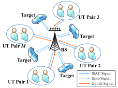
Figure 1: ​Illustration of a​ downlink/uplink NOMA-ISAC system.

II System Model

Consider a downlink/uplink NOMA-ISAC system as depicted in Figure 1, where a DFSAC BS is communicating with multiple UTs equipped with $N$ antennas each, while simultaneously sensing the targets in its surrounding environment. The BS operates in full duplex mode with two distinct sets of antennas, $M$ ($M\leqslant N$) transmit antennas and $M$ receive antennas, which are well-separated in space [4]. In this paper, the proposed system has the capability to serve up to $2M$ UTs, which outperforms the existing works [11, 21]. This expanded capacity will be justified in the subsequent analysis. To alleviate the system load, previous studies on NOMA have demonstrated the advantages of pairing users with distinct channel conditions [22, 13]. Building upon this understanding, we assume pairing an UT located near to the BS, $m$, with a cell-edge UT, $m^{\prime}$, to form a NOMA pair for $m=1,...,M$, and thus $M$ pairs are formed in total. For simplicity, we assume that the BS and UTs have full channel state information (CSI) and that the BS can perfectly eliminate the echo signal reflected by the UTs [9].

II-A Downlink ISAC

Consider a DFSAC signal matrix $\mathbf{X}=\left[{\mathbf{x}}_{1}\ldots{\mathbf{x}}_{L}\right]\in{\mathbbmss{C}}^{M\times L}$ sent from the BS, where $L$ represents the length of the communication frame/sensing pulse. In the context of sensing, ${\mathbf{x}}_{l}\in{\mathbbmss{C}}^{M\times 1}$ for $l=1,\ldots,L$ represents the sensing snapshot transmitted during the $l$th time slot. For communication purposes, ${\mathbf{x}}_{l}$ corresponds to the $l$th data symbol vector. Under the framework of MIMO-based ISAC, we can express the downlink signal matrix $\mathbf{X}$ as follows:

$$\mathbf{X}=\mathbf{P}\mathbf{S}=\mathbf{W}_{\rm{d}}\mathbf{\Xi}^{\frac{1}{2}}\mathbf{S},$$ (1)

where $\mathbf{P}=\mathbf{W}_{\rm{d}}\mathbf{\Xi}^{\frac{1}{2}}\in\mathbbmss{C}^{M\times M}$ denotes the downlink precoding matrix at the BS, $\mathbf{W}_{\rm{d}}=\left[\mathbf{w}_{{\rm{d}},1}\ldots\mathbf{w}_{{\rm{d}},M}\right]\in\mathbbmss{C}^{M\times M}$ contains the normalized precoders with $\lVert{\mathbf{w}}_{{\rm{d}},m}\rVert^{2}=1$ for $m=1,\ldots,M$, $\mathbf{\Xi}=\mathsf{diag}\left\{p_{1},...,p_{M}\right\}\succcurlyeq\mathbf{0}$ is the power allocation matrix subject to the power budget $\sum_{m=1}^{M}{p_{m}\leqslant p}$, and $\mathbf{S}=\left[{\mathbf{s}}_{1}\ldots{\mathbf{s}}_{M}\right]^{\mathsf{H}}\in{\mathbbmss{C}}^{M\times L}$ contains $M$ unit-power data streams intended for the $M$ pairs. Specifically, it follows that

$$\mathbf{s}_{m}=\sqrt{\alpha_{m}}\mathbf{s}_{\mathrm{d},m}+\sqrt{\alpha_{m^{\prime}}}\mathbf{s}_{\mathrm{d},m^{\prime}},$$ (2)

where $\mathbf{s}_{\mathrm{d},m}\in\mathbbmss{C}^{L\times 1}$ and $\mathbf{s}_{\mathrm{d},m^{\prime}}\in\mathbbmss{C}^{L\times 1}$ denote the unit-power information bearing signals to be transmitted to UT $m$ and UT $m^{\prime}$, respectively, and $\alpha_{m}$ and $\alpha_{m^{\prime}}$ denote the NOMA power allocation coefficients with $\alpha_{m}+\alpha_{m^{\prime}}=1$. The data streams are assumed to be independent with each other such that $L^{-1}\mathbf{S}\mathbf{S}^{\mathsf{H}}=\mathbf{I}_{M}$.

II-A1 Sensing Model

When transmitting the signal matrix $\mathbf{X}$ for target sensing, the BS receives the reflected echo signal matrix, which can be expressed as follows: [4, 9, 11]

$${\mathbf{Y}}_{\rm{s}}={\mathbf{G}}{\mathbf{X}}+{\mathbf{N}}_{\rm{s}},$$ (3)

where ${\mathbf{N}}_{\rm{s}}\in{\mathbbmss{C}}^{M\times L}$ is the additive white Gaussian noise (AWGN) matrix with each entry having zero mean and unit variance, and $\mathbf{G}=\left[{\mathbf{g}}_{1}\ldots{\mathbf{g}}_{M}\right]^{\mathsf{H}}\in{\mathbbmss{C}}^{M\times M}$ represents the target response matrix with ${\mathbf{g}}_{m}\in{\mathbbmss{C}}^{M\times 1}$ for $m=1,\ldots,M$ characterizing the target response from the transmit antenna array to the $m$th receive antenna. The target response matrix is modeled as [8, 4, 9]

$$\mathbf{G}=\sum\nolimits_{k}\beta_{k}{\mathbf{a}}\left(\theta_{k}\right){\mathbf{b}}^{\mathsf{H}}\left(\theta_{k}\right),$$ (4)

where $\beta_{k}\sim{\mathcal{CN}}\left(0,\sigma_{k}^{2}\right)$ denotes the complex amplitude of the $k$th target with the average strength of $\sigma_{k}^{2}$, ${\mathbf{a}}\left(\theta_{k}\right)\in{\mathbbmss{C}}^{M\times 1}$ and ${\mathbf{b}}\left(\theta_{k}\right)\in{\mathbbmss{C}}^{M\times 1}$ are the associated receive and transmit array steering vectors, respectively, and $\theta_{k}$ is its direction of arrival. Assuming that the receive antennas at the BS are widely separated, we have $\mathbf{g}_{m}\sim{\mathcal{CN}}\left({\mathbf{0}},\mathbf{R}\right)$ for $m=1,\ldots,M$ and ${\mathbb{E}}\left\{{\mathbf{g}}_{m}{\mathbf{g}}_{m^{\prime}}^{\mathsf{H}}\right\}={\mathbf{0}}$ for $m\neq m^{\prime}$ [4].

In contrast to the instantaneous target response matrix $\mathbf{G}$, the correlation matrix ${\mathbf{R}}\in{\mathbbmss{C}}^{M\times M}$ remains relatively stable over an extended period. Obtaining $\mathbf{R}$ is a straightforward task for the BS through long-term feedback. Therefore, for the purposes of our discussion, we assume that the BS has access to the correlation matrix $\mathbf{R}$, which is the assumption commonly made in the literature [8, 4, 9, 11].

The primary objective of sensing is to extract environmental information contained in the target response $\mathbf{G}$, such as the direction and reflection coefficient of each target, from the reflected echo signal ${\mathbf{Y}}_{\rm{s}}$ [8, 4, 9, 11]. This extraction of information is quantified by the mutual information (MI) between ${\mathbf{Y}}_{\rm{s}}$ and $\mathbf{G}$ conditioned on the DFSAC signal ${\mathbf{X}}$, which is commonly referred to as the sensing MI [4, 5]. From an information-theoretical perspective, the sensing performance is evaluated using the SR, defined as the sensing MI per unit time [23, 8, 9, 5]. Assuming that each DFSAC symbol lasts for 1 unit of time, the SR is expressed as follows:

$${\mathcal{R}}_{\rm{s}}=L^{-1}I\left({\mathbf{Y}}_{\rm{s}};\mathbf{G}|\mathbf{X}\right),$$ (5)

where $I\left(X;Y|Z\right)$ represents the MI between random variables $X$ and $Y$ conditioned on $Z$.

II-A2 Communication Model

By transmitting $\mathbf{X}$ to the UTs, the received signal matrix at UT $m$ is given by

$$\mathbf{Y}_{\mathrm{c},m}= \sqrt{\eta_{m}^{-1}p_{m}}\mathbf{H}_{\mathrm{d},m}\mathbf{w}_{{\rm{d}},m}\mathbf{s}_{m}^{\mathsf{H}}$$

$$+{\sum}_{i\neq m}{\sqrt{\eta_{m}^{-1}p_{i}}\mathbf{H}_{\mathrm{d},m}\mathbf{w}_{{\rm{d}},i}}\mathbf{s}_{i}^{\mathsf{H}}+\mathbf{N}_{m},$$ (6)

where $\eta_{m}$ denotes the large-scale path loss for UT $m$, ${\mathbf{H}}_{\mathrm{d},m}\in{\mathbbmss{C}}^{N\times M}$ is the downlink communication channel matrix with each element representing independent and identically distributed (i.i.d.) Rayleigh fading channel gains, and ${\mathbf{N}}_{m}\in{\mathbbmss{C}}^{N\times L}$ is the AWGN matrix with each entry having zero mean and unit variance.

After receiving $\mathbf{Y}_{{\rm{c}},m}$, the UT adopts a detection vector (equalizer) $\mathbf{v}_{\mathrm{d},m}\in{\mathbbmss{C}}^{N\times 1}$, and thus the UT’s observation can be rewritten as follows:

$$\mathbf{v}_{\mathrm{d},m}^{\mathsf{H}}\!\mathbf{Y}_{\mathrm{c},m}\! =\sqrt{\eta_{m}^{-1}p_{m}}\mathbf{v}_{\mathrm{d},m}^{\mathsf{H}}\mathbf{H}_{\mathrm{d},m}\mathbf{w}_{{\rm{d}},m}\mathbf{s}_{m}^{\mathsf{H}}$$

$$\!\!\!\!+\underset{\mathrm{IPI}}{\underbrace{{\sum}_{i\neq m}\!{\sqrt{\eta_{m}^{-1}p_{i}}\mathbf{v}_{\mathrm{d},m}^{\mathsf{H}}\mathbf{H}_{\mathrm{d},m}\mathbf{w}_{{\rm{d}},i}}\mathbf{s}_{i}^{\mathsf{H}}}}\!+\!\mathbf{v}_{\mathrm{d},m}^{\mathsf{H}}\mathbf{N}_{m}.$$ (7)

To eliminate the IPI, it’s necessary to fulfill the conditions $\mathbf{v}_{\mathrm{d},i}^{\mathsf{H}}\mathbf{H}_{\mathrm{d},i}\mathbf{w}_{\mathrm{d},m}=0$ and $\mathbf{v}_{\mathrm{d},i^{\prime}}^{\mathsf{H}}\mathbf{H}_{\mathrm{d},i^{\prime}}\mathbf{w}_{\mathrm{d},m}=0$ for $i=1,..,m-1,m+1,...,M$. In this context, from the perspective of designing $\mathbf{w}_{\mathrm{d},m}$, a total of $2(M-1)$ equations must be satisfied, while only $M$ variables are available. Consequently, unless the total number of UT pairs is no greater than $\frac{M}{2}+1$, it’s not feasible for a non-zero vector $\mathbf{w}_{\mathrm{d},m}$ to exist [22]. However, reducing the number of pairs will inevitably result in a reduction of the overall system throughput.

In order to overcome this problem, the concept of signal alignment can be applied, where the detection vectors are designed to satisfy the constraint $\mathbf{v}_{\mathrm{d},m}^{\mathsf{H}}\mathbf{H}_{\mathrm{d},m}=\mathbf{v}_{\mathrm{d},m^{\prime}}^{\mathsf{H}}\mathbf{H}_{\mathrm{d},m^{\prime}}$ [22]. By applying the signal alignment, the channels of the two UTs within the same pair are projected to a common direction, effectively reducing the dimension of the received signals, i.e., only $M-1$ equations need to be satisfied. This alignment enables the proposed system to accommodate $2M$ UTs, providing the potential to serve a larger number of users. The designs of such $\mathbf{v}_{\mathrm{d},m}$ and $\mathbf{v}_{\mathrm{d},m^{\prime}}$ as well as the preocoder $\mathbf{W}_{\rm{d}}$ will be detailed in the next section.

Based on the above analysis, the effective channel gains at UT $m$ and $m^{\prime}$ are expressed as $g_{m}=\eta_{m}^{-1}\left|\mathbf{v}_{\mathrm{d},m}^{\mathsf{H}}\mathbf{H}_{\mathrm{d},m}\mathbf{w}_{\mathrm{d},m}\right|^{2}$ and $g_{m^{\prime}}=\eta_{m^{\prime}}^{-1}\left|\mathbf{v}_{\mathrm{d},m^{\prime}}^{\mathsf{H}}\mathbf{H}_{\mathrm{d},m^{\prime}}\mathbf{w}_{\mathrm{d},m}\right|^{2}$, respectively. Because the path loss is positively correlated with the distance to the BS, i.e., $\eta_{m}^{-1}>\eta_{m^{\prime}}^{-1}$, and $\mathbf{v}_{\mathrm{d},m}^{\mathsf{H}}\mathbf{H}_{\mathrm{d},m}=\mathbf{v}_{\mathrm{d},m^{\prime}}^{\mathsf{H}}\mathbf{H}_{\mathrm{d},m^{\prime}}$, we have $g_{m}>g_{m^{\prime}}$. Therefore, according to the principle of NOMA, the two UTs from the same pair are ordered without any ambiguity, i.e., $\alpha_{m}<\alpha_{m^{\prime}}$. In this paper, we adopt a fixed set of power allocation coefficients. UT $m$ performs the SIC process by first eliminating the message of $m^{\prime}$ before decoding its own signals, while $m^{\prime}$ directly decode its own signals. Therefore, the SNR of UT $m$ and the signal-to-interference-plus-noise ratio (SINR) of UT $m^{\prime}$ are, respectively, given by

$$\gamma_{\mathrm{d},m} =\frac{\alpha_{m}\eta_{m}^{-1}p_{m}\left|\mathbf{v}_{\mathrm{d},m}^{\mathsf{H}}\mathbf{H}_{\mathrm{d},m}\mathbf{w}_{\mathrm{d},m}\right|^{2}}{\left\|\mathbf{v}_{\mathrm{d},m}\right\|^{2}},$$ (8)

$$\gamma_{\mathrm{d},m^{\prime}} =\frac{\alpha_{m^{\prime}}\eta_{m^{\prime}}^{-1}p_{m}\left|\mathbf{v}_{\mathrm{d},m\prime}^{\mathsf{H}}\mathbf{H}_{\mathrm{d},m\prime}\mathbf{w}_{\mathrm{d},m}\right|^{2}}{\alpha_{m}\eta_{m\prime}^{-1}p_{m}\left|\mathbf{v}_{\mathrm{d},m\prime}^{\mathsf{H}}\mathbf{H}_{\mathrm{d},m\prime}\mathbf{w}_{\mathrm{d},m}\right|^{2}+\left\|\mathbf{v}_{\mathrm{d},m^{\prime}}\right\|^{2}}.$$ (9)

Given the downlink NOMA-ISAC framework, we aim to analyze its S&C performance by evaluating the CR and SR, both of which are influenced by the precoding matrix $\mathbf{P}=\mathbf{W}_{\rm{d}}\mathbf{\Xi}^{\frac{1}{2}}$. However, finding an optimal $\mathbf{P}$ that can simultaneously maximize both metrics poses a challenge. To address this issue, we propose to explore three distinct scenarios for the downlink ISAC in Section III, which offer valuable insights into the system’s performance. The first scenario focuses on the S-C design, with a primary objective of optimizing the SR. The second scenario, C-C design, aims to maximize the CR. Lastly, we investigate the Pareto optimal design, which seeks to identify the Pareto boundary of the SR-CR rate region.

$$\mathbf{Y}_{\mathrm{BS}} =\underset{\mathbf{Y}_{\mathrm{BS}}^{\rm{c}}}{\underbrace{\sum\nolimits_{m=1}^{M}{\left(\sqrt{\alpha_{m}\eta_{m}^{-1}p_{\rm{c}}}\mathbf{H}_{\mathrm{u},m}\mathbf{w}_{{\rm{u}},m}\mathbf{s}_{\mathrm{u},m}^{\mathsf{H}}+\sqrt{\alpha_{m^{\prime}}\eta_{m^{\prime}}^{-1}p_{\rm{c}}}\mathbf{H}_{\mathrm{u},m^{\prime}}\mathbf{w}_{{\rm{u}},m^{\prime}}\mathbf{s}_{\mathrm{u},m^{\prime}}^{\mathsf{H}}\right)}}}+\mathbf{GX}_{\rm{s}}+\mathbf{N}_{\mathrm{u}}.$$ (10)

$$\mathbf{v}_{\mathrm{u},m}^{\mathsf{H}}\mathbf{Y}_{\mathrm{BS}}^{\rm{c}} =\left(\sqrt{\alpha_{m}\eta_{m}^{-1}p_{\rm{c}}}\mathbf{v}_{\mathrm{u},m}^{\mathsf{H}}\mathbf{H}_{\mathrm{u},m}\mathbf{w}_{{\rm{u}},m}\mathbf{s}_{\mathrm{u},m}^{\mathsf{H}}+\sqrt{\alpha_{m^{\prime}}\eta_{m^{\prime}}^{-1}p_{\rm{c}}}\mathbf{v}_{\mathrm{u},m}^{\mathsf{H}}\mathbf{H}_{\mathrm{u},m^{\prime}}\mathbf{w}_{{\rm{u}},m^{\prime}}\mathbf{s}_{\rm{u},m^{\prime}}^{H}\right)$$

$$~{}~{}~{}~{}+\underset{\mathrm{IPI}}{\underbrace{\sum\nolimits_{i\neq m}{\left(\sqrt{\alpha_{i}\eta_{i}^{-1}p_{\rm{c}}}\mathbf{v}_{\mathrm{u},m}^{\mathsf{H}}\mathbf{H}_{\mathrm{u},i}\mathbf{w}_{{\rm{u}},i}\mathbf{s}_{\mathrm{u},i}^{H}+\sqrt{\alpha_{i^{\prime}}\eta_{i^{\prime}}^{-1}p_{\rm{c}}}\mathbf{v}_{\mathrm{u},m}^{\mathsf{H}}\mathbf{H}_{\mathrm{u},i^{\prime}}\mathbf{w}_{{\rm{u}},i^{\prime}}\mathbf{s}_{\mathrm{u},i^{\prime}}^{\mathsf{H}}\right)}}}.$$ (11)

II-B Uplink ISAC

For the uplink case, the signal observed by the BS is given as (10), shown at the bottom of the this page, where $\mathbf{Y}_{\mathrm{BS}}^{\rm{c}}\in{\mathbbmss{C}}^{M\times L}$ is the communication signal, $p_{\rm{c}}$ reflects the power constraint of each UT pair, $\mathbf{H}_{\mathrm{u},m}\in{\mathbbmss{C}}^{M\times N}$ and $\mathbf{H}_{\mathrm{u},m^{\prime}}\in{\mathbbmss{C}}^{M\times N}$ denote the uplink communication channel matrices of UT $m$ and UT $m^{\prime}$, respectively, with elements representing i.i.d. Rayleigh fading channel gains, $\mathbf{w}_{{\rm{u}},m}\in{\mathbbmss{C}}^{N\times 1}$ and $\mathbf{w}_{{\rm{u}},m^{\prime}}\in{\mathbbmss{C}}^{N\times 1}$ denote the precoding vectors for UT $m$ and UT $m^{\prime}$, respectively, $\mathbf{s}_{\mathrm{u},m}=\left[s_{\mathrm{u},m,1}\ldots s_{\mathrm{u},m,L}\right]^{\mathsf{H}}\in{\mathbbmss{C}}^{L\times 1}$ and $\mathbf{s}_{\mathrm{u},m^{\prime}}=\left[s_{\mathrm{u},m^{\prime},1}\ldots s_{\mathrm{u},m^{\prime},L}\right]^{\mathsf{H}}\in{\mathbbmss{C}}^{L\times 1}$ are the unit-power communication messages sent by $m$ and $m^{\prime}$ to the BS, respectively, with the symbols sent at different time slots being uncorrelated, i.e., $\mathbb{E}\left\{\mathbf{s}_{\mathrm{u},m}\mathbf{s}_{\mathrm{u},m}^{\mathsf{H}}\right\}=\mathbb{E}\left\{\mathbf{s}_{\mathrm{u},m^{\prime}}\mathbf{s}_{\mathrm{u},m^{\prime}}^{\mathsf{H}}\right\}=\mathbf{I}_{L}$, $\mathbf{X}_{\rm{s}}=\left[\mathbf{x}_{{\rm{s}},1},\ldots,\mathbf{x}_{{\rm{s}},L}\right]\in{\mathbbmss{C}}^{M\times L}$ denotes the uplink sensing signal with $\mathbf{x}_{{\rm{s}},l}\in{\mathbbmss{C}}^{M\times 1}$ being the waveform at the $l$th time slot, and $\mathbf{N}_{\mathrm{u}}=\left[\mathbf{n}_{{\rm{u}},1},\ldots,\mathbf{n}_{{\rm{u}},L}\right]\in{\mathbbmss{C}}^{M\times L}$ is the AWGN matrix with each entry having zero mean and unit variance.

After receiving the above signal, the BS is tasked with decoding both the communication signal’s data information and the environmental information contained in the target response $\mathbf{G}$. To address both inter-functionality interference (IFI) and IUI, a two-stage SIC process can be employed [21, Fig. 2]. The outer-stage SIC focuses on handling the IFI, while the inner-stage SIC tackles the IUI. In the context of the outer-stage SIC, we consider two SIC orders. In the first SIC order, the BS initially detects the communication signal by treating the sensing signal as interference [9, 24]. Subsequently, the detected communication signal is subtracted from the superposed signal, with the remaining portion utilized for sensing the target response. In the second SIC order, the BS first senses the target response signal by treating the communication signal as interference. Then, the sensing signal is subtracted, leaving the remaining part for detecting the communication signal. It is evident that the first SIC order offers superior sensing performance, while the second SIC order yields improved communication performance. Therefore, we refer to these two SIC orders as the S-C design and C-C design, respectively, for the uplink ISAC. Within the inner-stage SIC, the messages for each UT are decoded. As the sum rate of each user group remains constant in uplink NOMA, regardless of the decoding order [22], we assume that the power allocation coefficients and the decoding order are identical to the downlink case, i.e., UT $m^{\prime}$ is decoded first in the inner-stage SIC process.

Importantly, prior to performing the inner-stage SIC, it’s imperative to initially mitigate the IPI within the communication signal. Therefore, in the following discussion, with the exclusion of the sensing signal and noise, we focus on the communication signal to introduce the process of IPI elimination through signal alignment. By applying the detection vector $\mathbf{v}_{\mathrm{u},m}\in{\mathbbmss{C}}^{M\times 1}$ to detect the message from the $m$th UT pair, the communication signal is expressed as (11), shown at the bottom of this page.

To remove the IPI, we need to satisfy $\mathbf{v}_{\mathrm{u},m}^{\mathsf{H}}\mathbf{H}_{\mathrm{u},i}\mathbf{w}_{{\rm{u}},i}=\mathbf{v}_{\mathrm{u},m}^{\mathsf{H}}\mathbf{H}_{\mathrm{u},i^{\prime}}\mathbf{w}_{{\rm{u}},i^{\prime}}=0$ for $\forall i\neq m$. By leveraging the concept of signal alignment, we impose the constraint $\mathbf{H}_{\mathrm{u},m}\mathbf{w}_{{\rm{u}},m}=\mathbf{H}_{\mathrm{u},m^{\prime}}\mathbf{w}_{{\rm{u}},m^{\prime}}$ on the precoding vectors. Specifically, we can design the precoding vectors as follows:

$$\left[\begin{matrix}\mathbf{w}_{\mathrm{u},m}^{\mathsf{H}}&\mathbf{w}_{\mathrm{u},m\prime}^{\mathsf{H}}\\ \end{matrix}\right]^{\mathsf{H}}=\mathbf{\Psi}_{m}\mathbf{r}_{m},$$ (12)

where the matrix $\bm{\Psi}_{m}$ has dimensions $2N\times(2N-M)$ and comprises the $2N-M$ right singular vectors of $\left[\begin{matrix}\mathbf{H}_{\mathrm{u},m}&-\mathbf{H}_{\mathrm{u},m^{\prime}}\ \end{matrix}\right]$ corresponding to its zero singular values, and $\mathbf{r}_{m}$ is a $\left(2N-M\right)\times 1$ vector which can be arbitrarily chosen and is used to constrain the total transmission power of each UT pair. Following the principle in [22], we set $\left\|\mathbf{r}_{m}\right\|^{2}=2$ to satisfy the power constraint:

$$p_{\mathrm{c}}\alpha_{m}\left\|\mathbf{w}_{\mathrm{u},m}\right\|^{2}+p_{\mathrm{c}}\alpha_{m^{\prime}}\left\|\mathbf{w}_{\mathrm{u},m^{\prime}}\right\|^{2}$$

$$~{}\leqslant p_{\mathrm{c}}\max\left(\alpha_{m},\alpha_{m^{\prime}}\right)\left(\left\|\mathbf{w}_{\mathrm{u},m}\right\|^{2}+\left\|\mathbf{w}_{\mathrm{u},m^{\prime}}\right\|^{2}\right)\leqslant 2p_{\mathrm{c}}.$$ (13)

By defining $\mathbf{Q}\triangleq\left[\mathbf{H}_{\mathrm{u},1}\mathbf{w}_{{\rm{u}},1},\ldots,\mathbf{H}_{\mathrm{u},M}\mathbf{w}_{{\rm{u}},M}\right]^{\mathsf{H}}\in\mathbbmss{C}^{M\times M}$, the normalized zero-forcing-based detection matrix is designed as follows:

$$\mathbf{V}_{\rm{u}}=\left[\mathbf{v}_{\mathrm{u},1},\ldots,\mathbf{v}_{\mathrm{u},M}\right]=\mathbf{Q}^{-1}\mathbf{D},$$ (14)

where $\mathbf{D}=\mathsf{diag}\left\{\frac{1}{\sqrt{\left(\mathbf{Q}^{-\mathsf{H}}\mathbf{Q}^{-1}\right)_{1,1}}},\ldots,\frac{1}{\sqrt{\left(\mathbf{Q}^{-\mathsf{H}}\mathbf{Q}^{-1}\right)_{M,M}}}\right\}$ is a diagonal matrix to ensure $\left\|\mathbf{v}_{\mathrm{u},m}\right\|^{2}=1$ for $m=1,\ldots,M$, and $\left(\mathbf{A}\right)_{m,m}$ refers to the $m$th element on the diagonal of the matrix $\mathbf{A}$. Therefore, the detected signal from the $m$th UT pair in (11) can be rewritten as follows:

$$\mathbf{v}_{\mathrm{u},m}^{\mathsf{H}}\mathbf{Y}_{\mathrm{BS}}^{\rm{c}}=\frac{\sqrt{\alpha_{m}\eta_{m}^{-1}p_{\rm{c}}}\mathbf{s}_{\mathrm{u},m}^{\mathsf{H}}+\sqrt{\alpha_{m^{\prime}}\eta_{m^{\prime}}^{-1}p_{\rm{c}}}\mathbf{s}_{u,m^{\prime}}^{H}}{\sqrt{\left(\mathbf{Q}^{-\mathsf{H}}\mathbf{Q}^{-1}\right)_{m,m}}}.$$ (15)

Having elucidated the fundamental model of the uplink ISAC, the performance of the two scenarios, the S-C design and the C-C design, will be comprehensively analyzed in Section IV.

III Downlink Performance

This section introduces three scenarios for the downlink ISAC: S-C design, C-C design, and Pareto optimal design. In each scenario, the SR, CR, and outage performance are investigated using the concept of signal alignment. The performance of FDSAC is provided as the baseline. Furthermore, the CR-SR regions achieved by ISAC and FDSAC are characterized.

III-A Sensing-Centric Design

III-A1 Performance of Sensing

Under the S-C design, the precoding matrix $\mathbf{P}$ is set to maximize the downlink SR ${\mathcal{R}}_{\rm{d},\rm{s}}$. To proceed, we characterize the SR as follows.

Lemma 1.

For a given $\mathbf{P}$, ${\mathcal{R}}_{\rm{d},\rm{s}}$ can be calculated as

$${\mathcal{R}}_{\rm{d},\rm{s}}=L^{-1}M\log_{2}\det\left({\mathbf{I}}_{M}+L{\mathbf{P}}^{\mathsf{H}}{\mathbf{R}}{\mathbf{P}}\right).$$ (16)

Proof:

Please refer to Appendix A. ∎

Under the S-C design, the precoding matrix satisfies

$$\mathbf{P}_{\rm{s}}=\operatorname*{argmax}_{\mathsf{tr}\left(\mathbf{PP}^{\mathsf{H}}\right)\leq p}{\log_{2}\det\left({\mathbf{I}}_{M}+L{\mathbf{P}}^{\mathsf{H}}{\mathbf{R}}{\mathbf{P}}\right)}.$$ (17)

For analytical tractability, we assume that ${\mathbf{R}}\succ{\mathbf{0}}$. The following theorem provides the exact expression of SR as well as its high-SNR approximation.

Theorem 1.

In the S-C design, the maximum downlink SR is given by

$$\mathcal{R}_{\mathrm{d},\mathrm{s}}^{\mathrm{s}}=ML^{-1}\sum\nolimits_{m=1}^{M}{\log_{2}\left(1+L\lambda_{m}s_{m}^{\star}\right)},$$ (18)

where $\left\{\lambda_{m}>0\right\}_{m=1}^{M}$ are the eigenvalues of matrix ${\mathbf{R}}$ and $s_{m}^{\star}=\max\left\{0,\frac{1}{\nu}-\frac{1}{L\lambda_{m}}\right\}$ with
$\sum_{m=1}^{M}\max\left\{0,\frac{1}{\nu}-\frac{1}{L\lambda_{m}}\right\}=p$. The maximum SR is achieved when ${\mathbf{P}}{\mathbf{P}}^{\mathsf{H}}=\mathbf{W}_{\mathrm{d}}\mathbf{\Xi W}_{\mathrm{d}}^{\mathsf{H}}={\mathbf{U}}{\bm{\Delta}}_{\rm{s}}{\mathbf{U}}^{\mathsf{H}}$, where ${\mathbf{U}}{\mathsf{diag}}\left\{\lambda_{1},\ldots,\lambda_{M}\right\}{\mathbf{U}}^{\mathsf{H}}$ represents the eigendecomposition (ED) of ${\mathbf{R}}$ and ${\bm{\Delta}}_{\rm{s}}={\mathsf{diag}}\left\{s_{1}^{\star},\ldots,s_{M}^{\star}\right\}$. When $p\rightarrow\infty$, the asymptotic SR satisfies

$$\mathcal{R}_{\mathrm{d},\mathrm{s}}^{\mathrm{s},\infty}\approx\frac{M^{2}}{L}\left(\log_{2}{p}+\frac{1}{M}\sum\nolimits_{m=1}^{M}\log_{2}\left(\frac{L\lambda_{m}}{M}\right)\right).$$ (19)

Proof:

Please refer to Appendix B. ∎

Remark 1.

The expression in (19) indicates that the high-SNR slope of the SR achieved under the S-C design is $\frac{M^{2}}{L}$.

Under the S-C design, it is important to note that the normalized precoder is chosen as $\mathbf{W}_{\rm{d}}=\mathbf{U}$. Since $\mathbf{U}$ is a unitary matrix, to apply the signal alignment, we can design the normalized precoding vector as $\mathbf{w}_{\rm{d},m}=\mathbf{u}_{m}$, where $\mathbf{u}_{m}$ represents the $m$th column of $\mathbf{U}$ with $\left\|\mathbf{u}_{m}\right\|=1$. In this case, the detection vectors can be found by solving the following equations:

$$\mathbf{H}_{\mathrm{d},m}^{\mathsf{H}}\mathbf{v}_{\mathrm{d},m}=\mathbf{u}_{m},\ \mathbf{H}_{\mathrm{d},m^{\prime}}^{\mathsf{H}}\mathbf{v}_{\mathrm{d},m^{\prime}}=\mathbf{u}_{m}.$$ (20)

Because $\mathbf{H}_{\mathrm{d},m}^{\mathsf{H}},\mathbf{H}_{\mathrm{d},m^{\prime}}^{\mathsf{H}}\in\mathbbmss{C}^{M\times N}$ are row full rank matrices, the equations are underdetermined and have infinitely many solutions. When $N=M$, $\mathbf{v}_{\mathrm{d},m}$ and $\mathbf{v}_{\mathrm{d},m^{\prime}}$ can be uniquely determined, i.e., $\mathbf{v}_{\mathrm{d},m}=\mathbf{H}_{\mathrm{d},m}^{-\mathsf{H}}\mathbf{u}_{m}$ and $\mathbf{v}_{\mathrm{d},m^{\prime}}=\mathbf{H}_{\mathrm{d},m^{\prime}}^{-\mathsf{H}}\mathbf{u}_{m}$.

III-A2 Performance of Communications

The communication performance will be evaluated in terms of CRs and outage performance. Firstly, we focus on CRs. The CRs of UT $m$ and $m^{\prime}$ under the S-C design are defined as follows:

$$\overline{\mathcal{R}}_{\mathrm{d},m}^{\mathrm{s}}=\log_{2}(1+\gamma_{\mathrm{d},m}^{\mathrm{s}}),\ \overline{\mathcal{R}}_{\mathrm{d},m^{\prime}}^{\mathrm{s}}=\log_{2}(1+\gamma_{\mathrm{d},m^{\prime}}^{\mathrm{s}}),$$ (21)

where $\gamma_{\mathrm{d},m}^{\mathrm{s}}=\frac{\alpha_{m}\eta_{m}^{-1}s_{m}^{\star}}{\left\|\mathbf{v}_{\mathrm{d},m}\right\|^{2}}$ and $\gamma_{\mathrm{d},m\prime}^{\mathrm{s}}=\frac{\alpha_{m^{\prime}}\eta_{m^{\prime}}^{-1}s_{m}^{\star}}{\alpha_{m}\eta_{m^{\prime}}^{-1}s_{m}^{\star}+\left\|\mathbf{v}_{\mathrm{d},m^{\prime}}\right\|^{2}}$. We utilize the ergodic CR (ECR), i.e., $\mathcal{R}_{\mathrm{d},m}^{\mathrm{s}}=\mathbb{E}\left\{\overline{\mathcal{R}}_{\mathrm{d},m}^{\mathrm{s}}\right\}$ and $\mathcal{R}_{\mathrm{d},m^{\prime}}^{\mathrm{s}}=\mathbb{E}\left\{\overline{\mathcal{R}}_{\mathrm{d},m^{\prime}}^{\mathrm{s}}\right\}$, to assess the communication performance. However, since finding analytical expressions of $\mathbf{v}_{\mathrm{d},m}$ and $\mathbf{v}_{\mathrm{d},m^{\prime}}$ is challenging when $N>M$, making the derivation of the exact ECRs difficult, we present upper bounds of $\mathcal{R}_{\mathrm{d},m}^{\mathrm{s}}$ and $\mathcal{R}_{\mathrm{d},m^{\prime}}^{\mathrm{s}}$ for the case $N>M$. Particularly, when $N=M$, the analytical expressions of $\mathbf{v}_{\mathrm{d},m}$ and $\mathbf{v}_{\mathrm{d},m^{\prime}}$ exist, and thus the exact closed-form expressions can be derived. The following lemma provides the analysis of the ECRs for UT $m$ and UT $m^{\prime}$.

Lemma 2.

The upper bounds for $\mathcal{R}_{\mathrm{d},m}^{\mathrm{s}}$ and $\mathcal{R}_{\mathrm{d},m^{\prime}}^{\mathrm{s}}$ follow

$$\tilde{\mathcal{R}}_{\mathrm{d},m}^{\mathrm{s}} =\int_{0}^{\infty}{\log_{2}\left(1+\alpha_{m}\eta_{m}^{-1}s_{m}^{\star}x\right)f_{\gamma}\left(x\right)dx},$$ (22a)

$$\tilde{\mathcal{R}}_{\mathrm{d},m\prime}^{\mathrm{s}} =\int_{0}^{\infty}{\log_{2}\left(1+\frac{\alpha_{m^{\prime}}\eta_{m^{\prime}}^{-1}s_{m}^{\star}x}{\alpha_{m}\eta_{m^{\prime}}^{-1}s_{m}^{\star}x+1}\right)f_{\gamma}\left(x\right)dx},$$ (22b)

where $f_{\gamma}\left(x\right)$ is the probability density function (PDF) of the largest eigenvalue of the complex Wishart matrix given in [25, Eq. (17)]. When $N=M$, the closed-form expressions of the ECRs for UT $m$ and UT $m^{\prime}$ are derived as follows:

$$\mathcal{R}_{\mathrm{d},m}^{\mathrm{s}} =\frac{1}{\ln 2}\exp\left(\frac{1}{\alpha_{m}\eta_{m}^{-1}s_{m}^{\star}}\right)\mathrm{Ei}\left(-\frac{1}{\alpha_{m}\eta_{m}^{-1}s_{m}^{\star}}\right),$$ (23a)

$$\mathcal{R}_{\mathrm{d},m\prime}^{\mathrm{s}} =\frac{1}{\ln 2}\exp\left(\frac{1}{\eta_{m^{\prime}}^{-1}s_{m}^{\star}}\right)\mathrm{Ei}\left(-\frac{1}{\eta_{m^{\prime}}^{-1}s_{m}^{\star}}\right)$$

$$-\frac{1}{\ln 2}\exp\left(\frac{1}{\alpha_{m}\eta_{m^{\prime}}^{-1}s_{m}^{\star}}\right)\mathrm{Ei}\left(-\frac{1}{\alpha_{m}\eta_{m^{\prime}}^{-1}s_{m}^{\star}}\right),$$ (23b)

where $\mathrm{Ei}\left(x\right)=\int_{-\infty}^{x}{\frac{\exp\left(t\right)}{t}dt}$ denotes the exponential integral.

Proof:

Please refer to Appendix C. ∎

Theorem 2.

Based on the results in Lemma 2, an upper bound of the downlink sum ECR under the S-C design is given by

$$\tilde{\mathcal{R}}_{\mathrm{d},\mathrm{c}}^{\mathrm{s}}=\sum\nolimits_{m=1}^{M}{\tilde{\mathcal{R}}_{\mathrm{d},m}^{\mathrm{s}}+\tilde{\mathcal{R}}_{\mathrm{d},m^{\prime}}^{\mathrm{s}}}.$$ (24)

Particularly, when $N=M$, the exact closed-form expression for the sum ECR is derived as

$$\mathcal{R}_{\mathrm{d},\mathrm{c}}^{\mathrm{s}}=\sum\nolimits_{m=1}^{M}{\mathcal{R}_{\mathrm{d},m}^{\mathrm{s}}+\mathcal{R}_{\mathrm{d},m^{\prime}}^{\mathrm{s}}}.$$ (25)

Corollary 1.

When $p\rightarrow\infty$, under the S-C design, the upper bound of the sum ECR satisfies

$$\tilde{\mathcal{R}}_{\mathrm{d},\mathrm{c}}^{\mathrm{s},\infty}\approx M\left(\log_{2}p-\log_{2}M+\int_{0}^{\infty}{\log_{2}xf_{\gamma}\left(x\right)dx}\right)$$

$$+\sum\nolimits_{m=1}^{M}{\log_{2}\eta_{m}^{-1}}.$$ (26)

In the scenario where $N=M$, the asymptotic sum ECR in the high-SNR regime reads

$$\mathcal{R}_{\mathrm{d},\mathrm{c}}^{\mathrm{s},\infty}\!\approx\!M\!\left(\!\log_{2}p\!-\!\log_{2}M\!-\!\frac{\mathcal{C}}{\ln 2}\right)\!+\!\sum\nolimits_{m=1}^{M}{\!\log_{2}\eta_{m}^{-1}},$$ (27)

where $\mathcal{C}$ denotes the Euler constant [26].

Proof:

When $p\rightarrow\infty$, we have $s_{m}^{\star}\approx\frac{p}{M}$. With the aid of ${\lim}_{x\rightarrow\infty}\log_{2}\left(1+x\right)\approx\log_{2}x$ and [26, Eq. (4.331.1)], the results can be derived. ∎

Remark 2.

The results in (1) and (27) suggest that the high-SNR slope of the sum ECR under the S-C design is $M$.

Turn now to the outage performance. The downlink OPs of UT $m$ and $m^{\prime}$ under the S-C design are defined as follows:

$$\mathcal{P}_{\mathrm{d},m}^{\mathrm{s}} =1-\mathrm{Pr}\left(\overline{\mathcal{R}}_{\mathrm{d},m}^{\mathrm{s}}>\mathcal{R}_{\mathrm{d},m}^{\mathrm{t}},\overline{\mathcal{R}}_{\mathrm{d},m^{\prime}}^{\mathrm{s}}>\mathcal{R}_{\mathrm{d},m^{\prime}}^{\mathrm{t}}\right),$$ (28)

$$\mathcal{P}_{\mathrm{d},m\prime}^{\mathrm{s}} =\mathrm{Pr}\left(\overline{\mathcal{R}}_{\mathrm{d},m^{\prime}}^{\mathrm{s}}<\mathcal{R}_{\mathrm{d},m^{\prime}}^{\mathrm{t}}\right),$$ (29)

where $\mathcal{R}_{\mathrm{d},m}^{\mathrm{t}}$ and $\mathcal{R}_{\mathrm{d},m^{\prime}}^{\mathrm{t}}$ denote the target rates of UT $m$ and UT $m^{\prime}$, respectively. The following theorem provides a pair of lower bounds for the OPs of $m$ and $m^{\prime}$, along with exact closed-form expressions in the case where $N=M$.

Theorem 3.

The lower bounds of $\mathcal{P}_{\mathrm{d},m}^{\mathrm{s}}$ and $\mathcal{P}_{\mathrm{d},m^{\prime}}^{\mathrm{s}}$ satisfy

$$\!\tilde{\mathcal{P}}_{\mathrm{d},m}^{\mathrm{s}}\!=\!F_{\lambda}\!\left(\frac{\varrho_{m}}{s_{m}^{\star}}\right)\!\!+\!F_{\lambda}\!\left(\frac{\varrho_{m^{\prime}}}{s_{m}^{\star}}\right)\!\!-\!F_{\lambda}\!\left(\frac{\varrho_{m}}{s_{m}^{\star}}\right)\!F_{\lambda}\!\left(\frac{\varrho_{m^{\prime}}}{s_{m}^{\star}}\right)\!,$$ (30a)

$$\!\tilde{\mathcal{P}}_{\mathrm{d},m\prime}^{\mathrm{s}}\!=\!F_{\lambda}\left(\frac{\varrho_{m^{\prime}}}{s_{m}^{\star}}\right),$$ (30b)

respectively, where $\varrho_{m}=\frac{2^{\mathcal{R}_{\mathrm{d},m}^{\mathrm{t}}}\!-1}{\alpha_{m}\eta_{m}^{-1}}$, $\varrho_{m^{\prime}}=\frac{2^{\mathcal{R}_{\mathrm{d},m^{\prime}}^{\mathrm{t}}}-1}{\eta_{m^{\prime}}^{-1}-2^{\mathcal{R}_{\mathrm{d},m^{\prime}}^{\mathrm{t}}}\alpha_{m}\eta_{m^{\prime}}^{-1}}$, and $F_{\lambda}\left(\cdot\right)$ denotes the cumulative distribution function (CDF) of the largest eigenvalue of the complex Wishart matrix given in [25, Eq. (9)]. When $N=M$, we can derive the exact expressions of the OPs as follows:

$$\mathcal{P}_{\mathrm{d},m}^{\mathrm{s}} =1-\exp\left(-\frac{\varrho_{m}+\varrho_{m^{\prime}}}{s_{m}^{\star}}\right),$$ (31a)

$$\mathcal{P}_{\mathrm{d},m\prime}^{\mathrm{s}} =1-\exp\left(-\frac{\varrho_{m^{\prime}}}{s_{m}^{\star}}\right)$$ (31b)

Proof:

Please refer to Appendix D. ∎

Corollary 2.

When $p\rightarrow\infty$, the lower bounds of the OPs under the S-C design satisfy

$$\tilde{\mathcal{P}}_{\mathrm{d},m}^{\mathrm{s},\infty} \approx\left(\frac{M}{p}\right)^{MN}\left(\varrho_{m}^{MN}+\varrho_{m^{\prime}}^{MN}\right),$$ (32a)

$$\tilde{\mathcal{P}}_{\mathrm{d},m\prime}^{\mathrm{s},\infty} \approx\left(\frac{M\varrho_{m^{\prime}}}{p}\right)^{MN},$$ (32b)

For the case $N=M$, the asymptotic OPs of UT $m$ and UT $m^{\prime}$ are given by

$$\mathcal{P}_{\mathrm{d},m}^{\mathrm{s},\infty}\approx\frac{M\left(\varrho_{m}+\varrho_{m^{\prime}}\right)}{p},\quad\mathcal{P}_{\mathrm{d},m^{\prime}}^{\mathrm{s},\infty}\approx\frac{M\varrho_{m^{\prime}}}{p}.$$ (33)

Proof:

When $p\rightarrow\infty$, we have $s_{m}^{\star}\approx\frac{p}{M}$. By utilizing ${\lim}_{x\rightarrow 0}F_{\lambda}\left(x\right)=x^{MN}$ [27, Eq. (16)] and ${\lim}_{x\rightarrow 0}\exp\left(-x\right)=1-x$ [26, Eq. (1.211.1)], the results can be obtained. ∎

Remark 3.

Based on the results in Corollary 2, under the S-C design, the lower bounds for the OPs of UT $m$ and UT $m^{\prime}$ exhibit a diversity order of $MN$. Additionally, when $N=M$, the exact OPs have a diversity order of one, indicating there is no error floor.

III-B Communications-Centric Design

In this subsection, we investigate the C-C design.

III-B1 Performance of Communications

Since $\mathbf{H}_{\mathrm{d},i}$ has the same statistical properties as $\mathbf{H}_{\mathrm{d},i}\mathbf{U}$ for $i\in\left\{m,m^{\prime}\right\}$, we can leverage the findings from Theorem 1 to design the C-C precoding marix as $\mathbf{P}=\mathbf{U}\bm{\Delta}_{\mathrm{c}}^{\frac{1}{2}}$, where $\bm{\Delta}_{\mathrm{c}}=\mathsf{diag}\left\{c_{1},\ldots,c_{M}\right\}$ satisfies $\sum_{m=1}^{M}c_{m}\leq p$ and $c_{m}\geq 0$ for $m=1,\ldots,M$. Hence, the optimal precoding matrix is given by

$$\mathbf{P}_{\rm{c}}\!=\operatorname*{argmax}_{\mathbf{P}=\mathbf{U\Delta}_{\mathrm{c}}^{1/2}} \sum\nolimits_{m=1}^{M}{\log_{2}\left(1\!+\!\frac{\alpha_{m}\eta_{m}^{-1}c_{m}}{\left\|\mathbf{v}_{\mathrm{d},m}\right\|^{2}}\right)}$$

$$+\log_{2}\left(1\!+\!\frac{\alpha_{m^{\prime}}\eta_{m^{\prime}}^{-1}c_{m}}{\alpha_{m}\eta_{m^{\prime}}^{-1}c_{m}+\left\|\mathbf{v}_{\mathrm{d},m^{\prime}}\right\|^{2}}\right).$$ (34)

Under the C-C design, the maximum sum CR achieved by $\mathbf{P}_{\rm{c}}$ are expressed as follows:

$$\overline{\mathcal{R}}_{\mathrm{d},\mathrm{c}}^{\mathrm{c}}=\sum\nolimits_{m=1}^{M} {\log_{2}\left(1+\frac{\alpha_{m}\eta_{m}^{-1}c_{m}^{\star}}{\left\|\mathbf{v}_{\mathrm{d},m}\right\|^{2}}\right)}$$

$$\!\!+\log_{2}\left(1+\frac{\alpha_{m^{\prime}}\eta_{m^{\prime}}^{-1}c_{m}^{\star}}{\alpha_{m}\eta_{m^{\prime}}^{-1}c_{m}^{\star}+\left\|\mathbf{v}_{\mathrm{d},m^{\prime}}\right\|^{2}}\right),$$ (35)

where $c_{m}^{\star}$ denotes the optimal power allocation for $m$th pair under the C-C design, and can be found by solving the following problem:

$$\underset{c_{m}}{\min}\,-\sum\nolimits_{m=1}^{M} {\log_{2}\left(1+\frac{\alpha_{m}\eta_{m}^{-1}c_{m}}{\left\|\mathbf{v}_{\mathrm{d},m}\right\|^{2}}\right)}$$

$$-\log_{2}\left(1+\frac{\alpha_{m^{\prime}}\eta_{m^{\prime}}^{-1}c_{m}}{\alpha_{m}\eta_{m^{\prime}}^{-1}c_{m}+\left\|\mathbf{v}_{\mathrm{d},m}\right\|^{2}}\right),$$

$$\mathrm{s}.\mathrm{t}.\ \sum\nolimits_{m=1}^{M} {c_{m}}-p=0,\quad c_{m}\geqslant 0,$$ (36)

which is convex and can be solved by using Karush–Kuhn–Tucker (KKT) conditions.

It is challenging to get a closed-form expression of the sum ECR $\mathcal{R}_{\mathrm{d},\mathrm{c}}^{\mathrm{c}}=\mathbb{E}\left\{\bar{\mathcal{R}}_{\mathrm{d},\mathrm{c}}^{\mathrm{c}}\right\}$. Hence, to get more insights, we study its high-SNR performance in the following lemma.

Lemma 3.

As $p\rightarrow\infty$, under the C-C design, an upper bound for the sum ECR is given by

$$\tilde{\mathcal{R}}_{\mathrm{d},\mathrm{c}}^{\mathrm{c},\infty}\approx M\left(\log_{2}p-\log_{2}M+\int_{0}^{\infty}{\log_{2}xf_{\gamma}\left(x\right)dx}\right)$$

$$+\sum\nolimits_{m=1}^{M}{\log_{2}\eta_{m}^{-1}}.$$ (37)

In the scenario where $N=M$, the asymptotic sum ECR in the high SNR-regime is derived as

$$\mathcal{R}_{\mathrm{d},\mathrm{c}}^{\mathrm{c},\infty}\approx M\left(\log_{2}p-\log_{2}M-\mathcal{C}\right)+\sum\nolimits_{m=1}^{M}{\log_{2}\eta_{m}^{-1}}.$$ (38)

Proof:

Similar to the proof of Corollary 1. ∎

Remark 4.

The results in (3) and (38) suggest that the high-SNR slope of the sum ECR under the C-C design is $M$.

Now we consider the OPs of UT $m$ and UT $m^{\prime}$, which are defined as follows:

$$\mathcal{P}_{\mathrm{d},m}^{\mathrm{c}} =1-\mathrm{Pr}\left(\overline{\mathcal{R}}_{\mathrm{d},m}^{\mathrm{c}}>\mathcal{R}_{\mathrm{d},m}^{\mathrm{t}},\overline{\mathcal{R}}_{\mathrm{d},m^{\prime}}^{\mathrm{c}}>\mathcal{R}_{\mathrm{d},m^{\prime}}^{\mathrm{t}}\right),$$ (39)

$$\mathcal{P}_{\mathrm{d},m\prime}^{\mathrm{c}} =\mathrm{Pr}\left(\overline{\mathcal{R}}_{\mathrm{d},m^{\prime}}^{\mathrm{c}}<\mathcal{R}_{\mathrm{d},m^{\prime}}^{\mathrm{t}}\right).$$ (40)

Lemma 4.

When $p\rightarrow\infty$, a pair of lower bounds for the OPs of UT $m$ and UT $m^{\prime}$ under the C-C design yields

$$\tilde{\mathcal{P}}_{\mathrm{d},m}^{\mathrm{c},\infty} \approx\left(\frac{M}{p}\right)^{MN}\left(\varrho_{m}^{MN}+\varrho_{m^{\prime}}^{MN}\right),$$ (41a)

$$\tilde{\mathcal{P}}_{\mathrm{d},m\prime}^{\mathrm{c},\infty} \approx\left(\frac{M\varrho_{m^{\prime}}}{p}\right)^{MN},$$ (41b)

For the case $N=M$, the asymptotic OPs of $m$ and $m^{\prime}$ in the high-SNR regime are given by

$$\mathcal{P}_{\mathrm{d},m}^{\mathrm{c},\infty}\approx\frac{M\left(\varrho_{m}+\varrho_{m^{\prime}}\right)}{p},\quad\mathcal{P}_{\mathrm{d},m^{\prime}}^{\mathrm{c},\infty}\approx\frac{M\varrho_{m^{\prime}}}{p}.$$ (42)

Proof:

Similar to the proof of Corollary 2. ∎

Remark 5.

According to the results presented in Lemma 4, the lower bounds for the OPs of UT $m$ and UT $m^{\prime}$ demonstrate a diversity order of $MN$ under the C-C design. Furthermore, when $N=M$, the exact OPs exhibit a diversity order of one.

Remark 6.

It can be observed that in high-SNR region, the CR and OPs achieved by the C-C design has the same asymptotic performance as those achieved by the S-C design.

III-B2 Performance of Sensing

When the precoding matrix $\mathbf{P}_{\mathrm{c}}$ is applied, the SR is expressed

$$\overline{\mathcal{R}}_{\mathrm{d},\mathrm{s}}^{\mathrm{c}}=ML^{-1}\sum\nolimits_{m=1}^{M}{\log_{2}\left(1+L\lambda_{m}c_{m}^{\star}\right)}.$$ (43)

To account for the statistics of $c_{m}^{\star}$, we define the average SR as $\mathcal{R}_{\mathrm{d},\mathrm{s}}^{\mathrm{c}}=\mathbb{E}\left\{\overline{\mathcal{R}}_{\mathrm{d},\mathrm{s}}^{\mathrm{c}}\right\}$ to numerically evaluate the average sensing performance. The high-SNR behaviour of $\mathcal{R}_{\mathrm{d},\mathrm{s}}^{\mathrm{c}}$ is described by the following theorem.

Theorem 4.

When $p\rightarrow\infty$, the asymptotic SR under the C-C design satisfies

$$\mathcal{R}_{\mathrm{d},\mathrm{s}}^{\mathrm{c},\infty}\approx\frac{M^{2}}{L}\left(\log_{2}{p}+\frac{1}{M}\sum\nolimits_{m=1}^{M}\log_{2}\left(\frac{L\lambda_{m}}{M}\right)\right).$$ (44)

Proof:

Similar to the proof of Theorem 1. ∎

Remark 7.

The expression presented in (44) indicates that the high-SNR slope of the SR achieved by the C-C design is $\frac{M^{2}}{L}$, and the SR under the C-C design yields the same asymptotic behaviour as that under the S-C design in high-SNR regime.

Remark 8.

Based on the findings in Remarks 6 and 7, we find that in the high-SNR regime, the C-C design converges to the S-C design, and vice versa.

III-C Pareto Optimal Design

In real-world scenarios, the precoding matrix $\mathbf{P}$ can be tailored to meet various quality of service requirements, leading to a tradeoff between communication and sensing performance in the downlink scenario. To assess this tradeoff, we use the Pareto boundary of the SR-CR region. The Pareto boundary is composed of SR-CR pairs where it is not possible to enhance one of the two rates without concomitantly diminishing the other [28]. Specifically, we design the precoding matrix as $\mathbf{P}={\mathbf{U}}{\mathsf{diag}}\left\{p_{1},\ldots,p_{M}\right\}$ with $\sum_{m=1}^{M}p_{m}\leq p$ and $p_{m}\geq 0$. Accordingly, any rate-tuple on the Pareto boundary of the downlink rate region can be obtained via solving the following optimization problem:

$$\max_{\mathbf{p},\mathcal{R}_{\rm{d}}}\ \ \mathcal{R}_{\rm{d}},$$ (45)

$$\mathrm{s}.\mathrm{t}.\ \ \mathcal{R}_{\rm{d},\mathrm{s}}\geq\rho\mathcal{R}_{\rm{d}},\,\mathcal{R}_{\rm{d},\mathrm{c}}\geq\left(1-\rho\right)\mathcal{R}_{\rm{d}},\,\mathbf{1}^{\mathsf{T}}\mathbf{p}\leq p,\,p_{m}\geq 0,$$

where $\rho\in\left[0,1\right]$ is a particular rate-profile parameter, and ${\mathbf{p}}=[p_{1},\ldots,p_{M}]^{\mathsf{T}}$. Problem (45) is convex and can be solved by using standard convex problem solvers, e.g., CVX. For a given value of $\rho$, let $\mathcal{R}_{\rm{d},\mathrm{s}}^{\rho}$ and $\mathcal{R}_{\rm{d},\mathrm{c}}^{\rho}$ represent the average SR and the sum ECR achieved by the corresponding optimal precoding matrix, respectively. Hence, we have $\mathcal{R}_{\mathrm{d},\mathrm{s}}^{\rho}\in\left[\mathcal{R}_{\mathrm{d},\mathrm{s}}^{\mathrm{c}},\mathcal{R}_{\mathrm{d},\mathrm{s}}^{\mathrm{s}}\right]$ and $\mathcal{R}_{\rm{d},\mathrm{c}}^{\rho}\in\left[\mathcal{R}_{\rm{d},\mathrm{c}}^{\rm{s}},\mathcal{R}_{\rm{d},\mathrm{c}}^{\rm{c}}\right]$ with $\mathcal{R}_{\rm{d},\mathrm{s}}^{1}=\mathcal{R}_{\rm{d},\mathrm{s}}^{\rm{s}}$ and $\mathcal{R}_{\rm{d},\mathrm{c}}^{0}=\mathcal{R}_{\rm{d},\mathrm{c}}^{\rm{c}}$, which yields the following corollary.

System	CR		SR
	$\mathcal{D}$	$\mathcal{S}$	$\mathcal{S}$
ISAC (S-C)	$1$	$M$	$M^{2}/L$
ISAC (C-C)	$1$	$M$	$M^{2}/L$
ISAC (Pareto Optimal)	$1$	$M$	$M^{2}/L$
FDSAC	$1$	$\kappa M$	$\left(1-\kappa\right)M^{2}/L$

TABLE I: Downlink Diversity Order ($\mathcal{D}$)
and High-SNR Slope ($\mathcal{S}$)

Corollary 3.

When the SNR is sufficiently high, for any given $\rho$, the corresponding optimal S&C performance is the same as the performance achieved by S-C and C-C design, i.e., they yield the same high-SNR slopes and diversity orders.

Proof:

This corollary can be proved by applying the conclusion in Remark 8 with the Sandwich theorem. ∎

Remark 9.

In the high-SNR regime, any downlink CR-SR pair on the Pareto boundary exhibits identical asymptotic behavior.

III-D Performance of FDSAC

The baseline scenario we are examining is FDSAC, which involves dividing the overall bandwidth into two sub-bands: one exclusively for sensing and the other for communications. Additionally, the total power is also partitioned into two portions for S&C, respectively. Specifically, we assume $\kappa$ fraction of the total bandwidth and $\mu$ fraction of the total power is used for communications. In this case, the SR and the sum ECR are given by

$$\mathcal{R}_{\mathrm{d},\mathrm{s}}^{\mathrm{f}}\! =\!\frac{M(1\!-\!\kappa)}{L}\!\max_{\sum_{m=1}^{M}{a_{m}}\leq(1-\mu)p}\sum\nolimits_{m=1}^{M}\!{\log_{2}\!\left(\!1\!+\!\frac{L\lambda_{m}}{1\!-\!\kappa}a_{m}\!\right)},$$ (46)

$$\mathcal{R}_{\mathrm{d},\mathrm{c}}^{\mathrm{f}}\! =\!\mathbb{E}\left\{\max_{\sum_{m=1}^{M}{b_{m}}\leq\mu p}\!\sum\nolimits_{m=1}^{M}{\!\kappa\log_{2}\!\left(\!1\!+\!\frac{\alpha_{m}\eta_{m}^{-1}b_{m}}{\kappa\left\|\mathbf{v}_{\mathrm{d},m}\right\|^{2}}\!\right)}\right.$$

$$~{}~{}~{}~{}~{}~{}~{}\left.+\kappa\log_{2}\!\left(\!1\!+\!\frac{\alpha_{m^{\prime}}\eta_{m^{\prime}}^{-1}b_{m}}{\alpha_{m}\eta_{m^{\prime}}^{-1}b_{m}\!+\!\kappa\left\|\mathbf{v}_{\mathrm{d},m^{\prime}}\right\|^{2}}\!\right)\!\right\}.$$ (47)

It is worth noting that $(\mathcal{R}_{\mathrm{d},\mathrm{s}}^{\mathrm{f}},\mathcal{R}_{\mathrm{d},\mathrm{c}}^{\mathrm{f}})$ can be discussed in the way we discuss $(\mathcal{R}_{\mathrm{d},\mathrm{s}}^{\mathrm{s}},\mathcal{R}_{\mathrm{d},\mathrm{c}}^{\mathrm{c}})$.

Upon concluding all the analyses of downlink case, we consolidate the outcomes pertaining to diversity order and high-SNR slope within Table I.

Remark 10.

The results in Table I suggest that FDSAC achieves the same diversity order as ISAC. However, the high-SNR slopes of both SR and CR achieved by FDSAC are smaller than those achieved by ISAC. This fact means that ISAC provides more degrees of freedom than FDSAC in terms of both communications and sensing.

III-E Rate Region Characterization

We now characterize the SR-CR region achieved by the downlink ISAC and FDSAC systems. In particular, let ${\mathcal{R}}_{\rm{d},\rm{s}}$ and ${\mathcal{R}}_{\rm{d},\rm{c}}$ denote the achievable SR and CR, respectively. Then, the rate regions achieved by ISAC and FDSAC are, respectively, given by

$$\mathcal{C}_{\mathrm{d},\mathrm{i}} =\!\left\{\left(\mathcal{R}_{\mathrm{d},\mathrm{s}},\mathcal{R}_{\mathrm{d},\mathrm{c}}\right)\left|\!\!\begin{array}[]{c}\mathcal{R}_{\mathrm{d},\mathrm{s}}\!\in\!\!\left[0,\mathcal{R}_{\mathrm{d},\mathrm{s}}^{\rho}\right],\mathcal{R}_{\mathrm{d},\mathrm{c}}\!\in\!\left[0,\mathcal{R}_{\mathrm{d},\mathrm{c}}^{\rho}\right],\\ \rho\in\left[0,1\right]\\ \end{array}\right.\!\!\right\},$$ (50)

$$\mathcal{C}_{\mathrm{d},\mathrm{f}} =\!\left\{\left(\mathcal{R}_{\mathrm{d},\mathrm{s}},\mathcal{R}_{\mathrm{d},\mathrm{c}}\right)\left|\!\!\begin{array}[]{c}\mathcal{R}_{\mathrm{d},\mathrm{s}}\!\in\!\left[0,\mathcal{R}_{\mathrm{d},\mathrm{s}}^{\mathrm{f}}\right],\mathcal{R}_{\mathrm{d},\mathrm{c}}\!\in\!\left[0,\mathcal{R}_{\mathrm{d},\mathrm{c}}^{\mathrm{f}}\right],\\ \kappa\in\left[0,1\right],\mu\in\left[0,1\right]\\ \end{array}\right.\!\!\right\}.$$ (53)

Theorem 5.

The above rate regions satisfy $\mathcal{C}_{\rm{d},\mathrm{f}}\subseteq\mathcal{C}_{\rm{d},\mathrm{i}}$.

Proof:

Please refer to Appendix E. ∎

According to Theorem 5, the downlink rate region achieved by ISAC entirely encompasses that achieved by FDSAC. This is mainly attributed to ISAC’s integrated exploitation of both spectrum and power resources.

IV Uplink Performance

In this section, we analyze the performance of uplink ISAC under the S-C and C-C designs according to the interference cancellation order of the two-stage SIC. Also, FDSAC is considered as the baseline and the uplink rate regions are provided.

IV-A Sensing-Centric Design

In the S-C design, the BS first decodes the communication signal $\{\mathbf{s}_{\mathrm{u},m},\mathbf{s}_{\mathrm{u},m^{\prime}}\}_{m=1}^{M}$ transmitted by UTs, considering the sensing signal $\mathbf{GX}_{\rm{s}}$ as interference. Then, the BS subtracts the decoded communication signal from the received signal, utilizing the remaining part for sensing the target response matrix $\mathbf{G}$.

IV-A1 Performance of Communications

From a worst-case design standpoint, the aggregate interference-plus-noise at $l$th time slot ${\bm{\xi}}_{m,l}=\mathbf{Gx}_{{\rm{s}},l}+\mathbf{n}_{{\mathrm{u}},l}$ is regarded as the Gaussian noise [24]. On this basis, we conclude the following lemma.

Lemma 5.

At the $l$th time slot, the uplink SNR of UT $m$ and SINR of UT $m^{\prime}$ are, respectively, given by

$$\gamma_{\mathrm{u},m,l}^{\mathrm{s}} =\frac{\alpha_{m}\eta_{m}^{-1}p_{\mathrm{c}}}{\left(\mathbf{Q}^{-\mathsf{H}}\mathbf{Q}^{-1}\right)_{m,m}\sigma_{\mathrm{s},l}^{2}},$$ (54)

$$\gamma_{\mathrm{u},m^{\prime},l}^{\mathrm{s}} =\frac{\alpha_{m^{\prime}}\eta_{m^{\prime}}^{-1}p_{\mathrm{c}}}{\alpha_{m}\eta_{m}^{-1}p_{\mathrm{c}}+\left(\mathbf{Q}^{-\mathsf{H}}\mathbf{Q}^{-1}\right)_{m,m}\sigma_{\mathrm{s},l}^{2}},$$ (55)

where $\sigma_{\mathrm{s},l}^{2}=\left|\mathbf{x}_{\mathrm{s},l}^{\mathsf{H}}\mathbf{Rx}_{\mathrm{s},l}\right|+1$.

Proof:

Utilizing the properties $\mathbf{g}_{n}\sim{\mathcal{CN}}\left({\mathbf{0}},\mathbf{R}\right)$ for $n=1,\ldots,N$ and $\mathbb{E}\left\{\mathbf{g}_{n}\mathbf{g}_{n^{\prime}}^{\mathsf{H}}\right\}=\mathbf{0}$ for $n\neq n^{\prime}$, as well as $\mathbf{n}_{\mathrm{u},l}\sim{\mathcal{CN}}\left({\mathbf{0}},\mathbf{I}\right)$, we derive the mean and variance of ${\bm{\xi}}_{m,l}$ as follows:

$$\mathbb{E}\left\{{\bm{\xi}}_{m,l}\right\} =\mathbf{0},$$ (56a)

$$\mathbb{E}\left\{{\bm{\xi}}_{m,l}{\bm{\xi}}_{m,l}^{\mathsf{H}}\right\} =\mathbb{E}\left\{\mathbf{Gx}_{\mathrm{s},l}\mathbf{x}_{\mathrm{s},l}^{\mathsf{H}}\mathbf{G}^{\mathsf{H}}\right\}+\mathbf{I}$$

$$=\left|\mathbf{x}_{\mathrm{s},l}^{\mathsf{H}}\mathbf{Rx}_{\mathrm{s},l}\right|\mathbf{I}+\mathbf{I}\triangleq\sigma_{\mathrm{s},l}^{2}\mathbf{I}.$$ (56b)

Therefore, for each UT pair, when treating the aggregate interference-plus-noise at the $l$th time slot as Gaussian noise, each of its elements exhibits a zero mean and a variance of $\sigma_{{\rm{s}},l}^{2}$. Since the detection vector $\mathbf{v}_{\mathrm{u},m}$ is normalized, the SNR and the SINR can be derived straightforwardly. ∎

Theorem 6.

The uplink sum ECR under the S-C design is given by

$$\mathcal{R}_{\mathrm{u},\mathrm{c},l}^{\mathrm{s}}=-\frac{1}{\ln 2}\sum\nolimits_{m=1}^{M}{\exp\left(\frac{\sigma_{\mathrm{s},l}^{2}}{p_{\mathrm{c}}\delta_{m}}\right)\mathrm{Ei}\left(-\frac{\sigma_{\mathrm{s},l}^{2}}{p_{\mathrm{c}}\delta_{m}}\right)},$$ (57)

where $\delta_{m}=\alpha_{m}\eta_{m}^{-1}+\alpha_{m^{\prime}}\eta_{m^{\prime}}^{-1}$. When $p_{\rm{c}}\rightarrow\infty$, the asymptotic ECR is expressed as follows:

$$\mathcal{R}_{\mathrm{u},\mathrm{c},l}^{\mathrm{s},\infty}\approx M\left(\log_{2}p_{\mathrm{c}}+\log_{2}\delta_{m}-\log_{2}\sigma_{\mathrm{s},l}^{2}-\mathcal{C}\right).$$ (58)

Proof:

Please refer to Appendix F. ∎

Remark 11.

(58) indicates that the high-SNR slope of the uplink sum ECR achieved by the S-C design is given by $M$.

The following theorem provides the closed-form expressions for the OP as well as its high-SNR approximations.

Theorem 7.

Under the uplink S-C design, the OP for the $m$th UT pair is given by

$$\mathcal{P}_{\mathrm{u},m,l}^{\mathrm{s}}=1-\exp\left(-\sigma_{\mathrm{s},l}^{2}\frac{2^{\mathcal{R}_{\mathrm{u}}^{\mathrm{t}}}-1}{p_{\mathrm{c}}\delta_{m}}\right).$$ (59)

where $\mathcal{R}_{\mathrm{u}}^{\mathrm{t}}$ denotes the target rate for the $m$th pair. When $p_{\rm{c}}\rightarrow\infty$, its high-SNR approximation satisfies

$$\mathcal{P}_{\mathrm{u},m,l}^{\mathrm{s},\infty}\approx\sigma_{\mathrm{s},l}^{2}\frac{2^{\mathcal{R}_{\mathrm{u}}^{\mathrm{t}}}-1}{p_{\mathrm{c}}\delta_{m}}.$$ (60)

Proof:

The OP of the $m$th UT pair is calculated as

$$\mathcal{P}_{\mathrm{u},m,l}^{\mathrm{s}} =\mathrm{Pr}\left(\frac{1}{\left(\mathbf{Q}^{-\mathsf{H}}\mathbf{Q}^{-1}\right)_{m,m}}<\sigma_{\mathrm{s},l}^{2}\frac{2^{\mathcal{R}_{\mathrm{u}}^{\mathrm{t}}}-1}{p_{\mathrm{c}}\delta_{m}}\right)$$

$$=F_{Q}\left(\sigma_{\mathrm{s},l}^{2}\frac{2^{\mathcal{R}_{\mathrm{u}}^{\mathrm{t}}}-1}{p_{\mathrm{c}}\delta_{m}}\right),$$ (61)

where $F_{Q}\left(x\right)$ denotes the CDF of $\frac{1}{\left(\mathbf{Q}^{-\mathsf{H}}\mathbf{Q}^{-1}\right)_{m,m}}$. Since $\frac{1}{\left(\mathbf{Q}^{-\mathsf{H}}\mathbf{Q}^{-1}\right)_{m,m}}$ is exponentially distributed [22, 29], we have $F_{Q}\left(\sigma_{\mathrm{s},l}^{2}\frac{2^{\mathcal{R}_{\mathrm{u}}^{\mathrm{t}}}-1}{p_{\mathrm{c}}\delta_{m}}\right)=1-\exp\left(-\sigma_{\mathrm{s},l}^{2}\frac{2^{\mathcal{R}_{\mathrm{u}}^{\mathrm{t}}}-1}{p_{\mathrm{c}}\delta_{m}}\right)$. When $p_{\rm{c}}\rightarrow\infty$, by utilizing the property $\lim_{x\rightarrow 0}\exp\left(-x\right)=1-x$, we can easily obtain (60). ∎

Remark 12.

According to the result in (60), the diversity order for the OP achieved by the uplink S-C design is given by one.

IV-A2 Performance of Sensing

Removing the decoded communication signal from the received signal, we now focus on the rest part which is used for sensing. The SR is dependent on the sensing signal $\mathbf{X}_{\mathrm{s}}$ and the maximum achievable uplink SR by S-C design is expressed as

$$\mathcal{R}_{\mathrm{u},\mathrm{s}}^{\mathrm{s}}\!=\!\max_{\mathsf{tr}\left(\mathbf{X}_{\mathrm{s}}\mathbf{X}_{\mathrm{s}}^{\mathsf{H}}\right)\leq Lp_{s}}\!ML^{-1}\log_{2}\det\left(\mathbf{I}_{M}\!+\!\mathbf{X}_{\mathrm{s}}^{\mathsf{H}}\mathbf{RX}_{\mathrm{s}}\right),$$ (62)

where $p_{\rm{s}}$ represents the per-symbol power budget for the uplink sensing signal.

Theorem 8.

The maximum SR achieved under the S-C design is given by

$$\mathcal{R}_{\mathrm{u},\mathrm{s}}^{\mathrm{s}}=ML^{-1}\sum\nolimits_{m=1}^{M}{\log_{2}\left(1+\lambda_{m}\zeta_{m}^{\mathrm{s}}\right)},$$ (63)

where $\zeta_{m}^{\mathrm{s}}=\max\left\{0,\frac{1}{\nu}-\frac{1}{\lambda_{m}}\right\}$ with $\sum_{m=1}^{M}\max\left\{0,\frac{1}{\nu}-\frac{1}{\lambda_{m}}\right\}=Lp_{\rm{s}}$. The maximum SR is achieved when $\mathbf{X}_{\mathrm{s}}\mathbf{X}_{\mathrm{s}}^{\mathsf{H}}={\mathbf{U}}{\bm{\Delta}}_{\varepsilon}^{\rm{s}}{\mathbf{U}}^{\mathsf{H}}$, where ${\bm{\Delta}}_{\varepsilon}^{\rm{s}}={\mathsf{diag}}\left\{\zeta_{1}^{\mathrm{s}},\ldots,\zeta_{M}^{\mathrm{s}}\right\}$. When $p_{\rm{s}}\rightarrow\infty$, the asymptotic SR is derived as follows:

$$\mathcal{R}_{\mathrm{u},\mathrm{s}}^{\mathrm{s},\infty}\approx\frac{M^{2}}{L}\left(\log_{2}{p_{\rm{s}}}+\frac{1}{M}\sum\nolimits_{m=1}^{M}\log_{2}\left(\frac{L\lambda_{m}}{M}\right)\right).$$ (64)

Proof:

Similar to the proof of Theorem 1. ∎

Remark 13.

The high-SNR slope of the uplink SR achieved under the S-C design is $\frac{M^{2}}{L}$.

IV-B Communications-Centric Design

In the C-C design, the target response signal is initially estimated by treating the communication signal as interference, followed by decoding the communication signals of UT $m$ and UT $m^{\prime}$ after removing the sensing signal.

IV-B1 Performance of Sensing

From a worst-case design standpoint, the aggregate interference-plus-noise $\mathbf{\Phi}=\sum\nolimits_{m=1}^{M}\left(\sqrt{\alpha_{m}\eta_{m}^{-1}p_{\rm{c}}}\mathbf{H}_{\mathrm{u},m}\mathbf{w}_{\mathrm{u},m}\mathbf{s}_{\mathrm{u},m}^{\mathsf{H}}+\right.$ $\left.\sqrt{\alpha_{m^{\prime}}\eta_{m^{\prime}}^{-1}p_{\rm{c}}}\mathbf{H}_{\mathrm{u},m^{\prime}}\mathbf{w}_{\mathrm{u},m^{\prime}}\mathbf{s}_{u,m^{\prime}}^{H}\right)+\mathbf{N}_{\mathrm{u}}$ can be treated as the Gaussian noise [24]. The uplink SR under the C-C design is provided in the following lemma.

Lemma 6.

The maximum achievable uplink SR by the C-C design is expressed as follows:

$$\mathcal{R}_{\mathrm{u},\mathrm{s}}^{\mathrm{c}}\!=\!\max_{\mathsf{tr}\left(\mathbf{X}_{\mathrm{s}}\mathbf{X}_{\mathrm{s}}^{\mathsf{H}}\right)\leq Lp_{s}}\!ML^{-1}\!\log_{2}\det\!\left(\mathbf{I}_{M}\!+\!\sigma_{\mathrm{c}}^{2}\mathbf{X}_{\mathrm{s}}^{\mathsf{H}}\mathbf{RX}_{\mathrm{s}}\right),$$ (65)

where $\sigma_{\mathrm{c}}^{2}=p_{\mathrm{c}}\sum\nolimits_{m=1}^{M}{\phi_{m}}+1$.

Proof:

Please refer to Appendix G. ∎

Theorem 9.

The exact expression of the maximum SR under the C-C design is given by

$$\mathcal{R}_{\mathrm{u},\mathrm{s}}^{\mathrm{c}}=ML^{-1}\sum\nolimits_{m=1}^{M}{\log_{2}\left(1+\sigma_{\mathrm{c}}^{-2}\lambda_{m}\zeta_{m}^{\rm{c}}\right)},$$ (66)

where $\zeta_{m}^{\mathrm{c}}=\max\left\{0,\frac{1}{\nu}-\frac{\sigma_{\mathrm{c}}^{2}}{\lambda_{m}}\right\}$ with $\sum_{m=1}^{M}\max\left\{0,\frac{1}{\nu}-\frac{\sigma_{\mathrm{c}}^{2}}{\lambda_{m}}\right\}=Lp_{\rm{s}}$. The maximum SR is achieved when $\mathbf{X}_{\mathrm{s}}\mathbf{X}_{\mathrm{s}}^{\mathsf{H}}={\mathbf{U}}{\bm{\Delta}}_{\varepsilon}^{\rm{c}}{\mathbf{U}}^{\mathsf{H}}$, where ${\bm{\Delta}}_{\varepsilon}^{\rm{c}}={\mathsf{diag}}\left\{\zeta_{1}^{\mathrm{c}},\ldots,\zeta_{M}^{\mathrm{c}}\right\}$.When $p_{\rm{s}}\rightarrow\infty$, the asymptotic SR satisfies

$$\mathcal{R}_{\mathrm{u},\mathrm{s}}^{\mathrm{c},\infty}\approx\frac{M^{2}}{L}\left(\log_{2}{p_{\rm{s}}}+\frac{1}{M}\sum\nolimits_{m=1}^{M}\log_{2}\left(\frac{L\lambda_{m}}{\sigma_{\mathrm{c}}^{2}M}\right)\right).$$ (67)

Proof:

Similar to the proof of Theorem 1. ∎

Remark 14.

The high-SNR slope of the SR achieved under the uplink C-C design is $\frac{M^{2}}{L}$.

IV-B2 Performance of Communications

After the target response is estimated, the sensing echo signal $\mathbf{G}\mathbf{X}$ can be subtracted from the received superposed S&C signal. Therefore, under the C-C design, the SNR for UT $m$ and the SINR for UT $m^{\prime}$ are, respectively, given by

$$\gamma_{\mathrm{u},m}^{\mathrm{c}}=\frac{\alpha_{m}\eta_{m}^{-1}p_{\mathrm{c}}}{\left(\mathbf{Q}^{-\mathsf{H}}\mathbf{Q}^{-1}\right)_{m,m}},$$ (68)

$$\gamma_{\mathrm{u},m^{\prime}}^{\mathrm{c}}=\frac{\alpha_{m^{\prime}}\eta_{m^{\prime}}^{-1}p_{\mathrm{c}}}{\alpha_{m}\eta_{m}^{-1}p_{\mathrm{c}}+\left(\mathbf{Q}^{-\mathsf{H}}\mathbf{Q}^{-1}\right)_{m,m}}.$$ (69)

Theorem 10.

The uplink sum ECR under the C-C design is given by

$$\mathcal{R}_{\mathrm{u},\mathrm{c}}^{\mathrm{c}}=-\frac{1}{\ln 2}\sum\nolimits_{m=1}^{M}{\exp\left(\frac{1}{p_{\mathrm{c}}\delta_{m}}\right)\mathrm{Ei}\left(-\frac{1}{p_{\mathrm{c}}\delta_{m}}\right)}.$$ (70)

When $p_{\rm{c}}\rightarrow\infty$, the high-SNR approximation of the sum ECR is derived as follows:

$$\mathcal{R}_{\mathrm{u},\mathrm{c}}^{\mathrm{c},\infty}\approx M\left(\log_{2}p_{\mathrm{c}}+\log_{2}\delta_{m}-\mathcal{C}\right).$$ (71)

Proof:

Similar to the proof of Theorem 6. ∎

Remark 15.

The results in (71) suggest that the high-SNR slope of the uplink sum ECR in the C-C design is $M$.

We next investigate the uplink outage performance under the C-C design.

Theorem 11.

The closed-form expression of OP for the $m$th UT pair is given by

$$\mathcal{P}_{\mathrm{u},m}^{\mathrm{c}}=1-\exp\left(-\frac{2^{\mathcal{R}_{\mathrm{u}}^{\mathrm{t}}}-1}{p_{\mathrm{c}}\delta_{m}}\right).$$ (72)

When $p_{\rm{c}}\rightarrow\infty$, its high-SNR approximation satisfies

$$\mathcal{P}_{\mathrm{u},m}^{\mathrm{c},\infty}\approx\frac{2^{\mathcal{R}_{\mathrm{u}}^{\mathrm{t}}}-1}{p_{\mathrm{c}}\delta_{m}}.$$ (73)

Proof:

Similar to the proof of Theorem 7. ∎

Remark 16.

According to the results in (73), a diversity of one is achievable for the OP of the $m$th UT pair under the C-C design.

According to the aforementioned analysis, we can draw the following conclusion.

Remark 17.

The SIC order does not affect the high-SNR slopes of both the CR and SR, nor does it affect the diversity order. However, it does have an impact on the performances by modifying the high-SNR power offsets and array gains [30].

System	CR		SR
	$\mathcal{D}$	$\mathcal{S}$	$\mathcal{S}$
ISAC (S-C)	$1$	$M$	$M^{2}/L$
ISAC (C-C)	$1$	$M$	$M^{2}/L$
ISAC (Time-Sharing)	$1$	$M$	$M^{2}/L$
FDSAC	$1$	$\kappa M$	$\left(1-\kappa\right)M^{2}/L$

TABLE II: Uplink Diversity Order ($\mathcal{D}$)
and High-SNR Slope ($\mathcal{S}$)

IV-C Rate Region Characterization

We now characterize the uplink SR-CR region achieved by the NOMA-ISAC. By utilizing the time-sharing strategy [30], we apply the S-C design with probability $\tau$ and the C-C design with probability $1-\tau$. For a given $\tau$, the achievable rate tuple is represented by $\left(\mathcal{R}_{\mathrm{u},\mathrm{s}}^{\tau},\mathcal{R}_{\mathrm{u},\mathrm{c}}^{\tau}\right)$, where $\mathcal{R}_{\mathrm{u},\mathrm{s}}^{\tau}=\tau\mathcal{R}_{\mathrm{u},\mathrm{s}}^{\mathrm{s}}+\left(1-\tau\right)\mathcal{R}_{\mathrm{u},\mathrm{s}}^{\mathrm{c}}$ and $\mathcal{R}_{\mathrm{u},\mathrm{c}}^{\tau}=\tau\mathcal{R}_{\mathrm{u},\mathrm{c}}^{\mathrm{s}}+\left(1-\tau\right)\mathcal{R}_{\mathrm{u},\mathrm{c}}^{\mathrm{c}}$. Let $\mathcal{R}_{\mathrm{u},\mathrm{s}}$ and $\mathcal{R}_{\mathrm{u},\mathrm{c}}$ denote the achievable SR and CR, respectively. Then, the rate region achieved by uplink ISAC follows

$$\mathcal{C}_{\mathrm{u},\mathrm{i}}\!=\!\left\{\!\left(\mathcal{R}_{\mathrm{u},\mathrm{s}},\mathcal{R}_{\mathrm{u},\mathrm{c}}\right)\left|\!\!\begin{array}[]{c}\mathcal{R}_{\mathrm{u},\mathrm{s}}\!\in\!\left[0,\mathcal{R}_{\mathrm{u},\mathrm{s}}^{\tau}\right],\mathcal{R}_{\mathrm{u},\mathrm{c}}\!\in\!\left[0,\mathcal{R}_{\mathrm{u},\mathrm{c}}^{\tau}\right],\\ \tau\in\left[0,1\right]\\ \end{array}\right.\!\!\!\right\}.$$ (76)

Remark 18.

Exploiting the Sandwich theorem, we obtain that any rate-tuple achieved by the time-sharing strategy yields the same high-SNR slopes and diversity order.

IV-D Performance of FDSAC

We also consider uplink FDSAC as the baseline scenario, where a fraction $\kappa\in\left[0,1\right]$ of the total bandwidth is allocated for communications, while the remaining fraction $1-\kappa$ of the bandwidth is allocated for sensing. In this case, the sum ECR and the SR of FDSAC satisfy

$$\mathcal{R}_{\mathrm{u},\mathrm{c}}^{\mathrm{f}} =\!\sum\nolimits_{m=1}^{M}{\mathbb{E}\left\{\kappa\log_{2}\left(1\!+\!\frac{p_{\mathrm{c}}\delta_{m}}{\kappa\left(\mathbf{Q}^{-1}\mathbf{Q}^{-\mathsf{H}}\right)_{m,m}}\right)\right\}},$$ (77)

$$\mathcal{R}_{\mathrm{u},\mathrm{s}}^{\mathrm{f}} =\frac{\left(1-\kappa\right)M}{L}\sum\nolimits_{m=1}^{M}{\log_{2}\left(1+\frac{\lambda_{m}\zeta_{m}^{\mathrm{s}}}{1-\kappa}\right)}.$$ (78)

It is worth noting that $(\mathcal{R}_{\mathrm{u},\mathrm{c}}^{\mathrm{f}},\mathcal{R}_{\mathrm{u},\mathrm{s}}^{\mathrm{f}})$ can be discussed in the way we discuss $(\mathcal{R}_{\mathrm{u},\mathrm{c}}^{\mathrm{c}},\mathcal{R}_{\mathrm{u},\mathrm{s}}^{\mathrm{s}})$.

Upon concluding all the analyses of uplink case, we consolidate the outcomes pertaining to diversity order and high-SNR slope within Table II.

Remark 19.

The results in Table II suggest that the uplink ISAC and FDSAC achieve the same diversity order, while ISAC achieves larger high-SNR slopes in terms of both SR and CR compared to FDSAC, indicating that ISAC provides more degrees of freedom in terms of both communications and sensing.

Finally, the rate region achieved by FDSAC is given by

$$\mathcal{C}_{\mathrm{u},\mathrm{f}}\!=\!\left\{\left(\mathcal{R}_{\mathrm{u},\mathrm{s}},\mathcal{R}_{\mathrm{u},\mathrm{c}}\right)\left|\!\!\begin{array}[]{c}\mathcal{R}_{\mathrm{u},\mathrm{s}}\!\in\!\left[0,\mathcal{R}_{\mathrm{u},\mathrm{s}}^{\mathrm{f}}\right],\mathcal{R}_{\mathrm{u},\mathrm{c}}\!\in\!\left[0,\mathcal{R}_{\mathrm{u},\mathrm{c}}^{\mathrm{f}}\right]\\ ,\kappa\in\left[0,1\right]\\ \end{array}\right.\!\!\!\right\}.$$ (81)

V Numerical Results

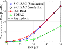
(a) Sum ECR.

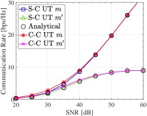
(b) ECR of UT $m$ and $m^{\prime}$.

Figure 2: Downlink communications rate.

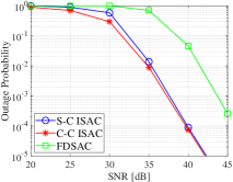
(a) OP of the sum CR.

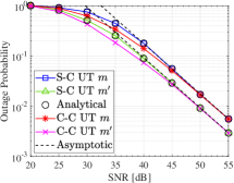
(b) OP of UT $m$ and UT $m^{\prime}$.

Figure 3: Downlink outage probability.

In this section, numerical results are provided to evaluate the S&C performance of ISAC systems and verify the derived analytical results. Without otherwise specification, the simulation parameter settings are defined as follows: $M=N=4$, $L=30$, $\kappa=\mu=0.5$, the NOMA power allocation coefficients are $\alpha_{m}=0.2$ and $\alpha_{m^{\prime}}=0.8$, the path loss are $\eta_{m}^{-1}=1\times 10^{-2}$ and $\eta_{m^{\prime}}^{-1}=2.5\times 10^{-3}$, and the eigenvalues of $\mathbf{R}$ are given by $\{1,0.1,0.05,0.01\}$.

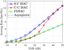
Figure 4: Downlink sensing rate.

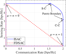
Figure 5: Downlink rate region.

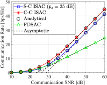
(a) Sum ECR.

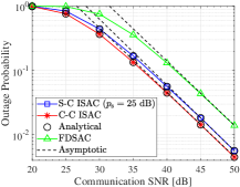
(b) OP of an UT pair.

Figure 6: Uplink communications performance.

V-A Downlink

Fig. 2(a) plots the downlink sum ECR versus the transmit SNR $p$. It can be seen that C-C ISAC achieves the best performance while FDSAC achieves the lowest sum ECR. The derived analytical results of sum ECR under the S-C design match the simulation results well, while the asymptotic results precisely track the simulation results in the high-SNR region. In Fig. 2(b), the ECR of UT $m$ and $m^{\prime}$ are respectively illustrated. We can observe that the ECR of UT $m$ increases linearly when SNR goes high, while UT $m^{\prime}$ converges to a upper bound. Fig. 3 displays the downlink outage performance. In Fig. 3(a), which shows the OP for the sum CR with a target rate of $8$ bps/Hz, C-C ISAC exhibits the lowest OP, while FDSAC demonstrates the highest. The OPs for UT $m$ and $m^{\prime}$, with the target rates $\mathcal{R}_{\rm{d},m}^{\rm{t}}\!=\!\mathcal{R}_{\rm{d},m^{\prime}}^{\rm{t}}\!=\!1$ bps/Hz, are presented in Fig. 3(b), confirming the validity of the analytical and asymptotic results. By observing Fig. 2 and Fig. 3, we find that the S-C ISAC and the C-C ISAC have the same high-SNR performance, which is consistent with the statement in Remark 6.

Fig. 5 shows the downlink sensing performance. We can observe that S-C ISAC exhibits the most superior SR performance, while the performance achieved by FDSAC is still the worst. By jointly examining Fig. 2, Fig. 3 and Fig. 5 together, it can be observed that in high SNR regime, the downlink communication and sensing performance of both the S-C ISAC and the C-C ISAC exhibit a similarity, aligning with the conclusion drawn in Remark 8. Moreover, it is evident that ISAC achieves larger high-SNR slopes than FDSAC in terms of both downlink CR and SR, while they achieve the same diversity order, demonstrating the claims stated in Remark 10.

In Fig. 5, the downlink SR-CR regions attained by the two systems with $p=25$ dB are displayed: ISAC system (presented in (50)) and the baseline FDSAC system (presented in (53)). The two marked points on the graph represent the S-C and C-C designs, respectively. The curve section connecting these two points represents the Pareto boundary of downlink ISAC’s rate region, which was derived by solving the problem (45) for values of $\rho$ ranging from $1$ to $0$. It is noteworthy that the rate region achieved by downlink FDSAC is entirely contained within that of downlink ISAC, justifying the correctness of Theorem 5.

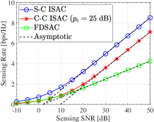
Figure 7: Uplink sensing rate.

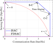
Figure 8: Uplink rate region, $p_{\rm{c}}=p_{\rm{u}}=25$ dB.

V-B Uplink

Then moving on to the uplink results, we examine Fig. 6(a) and Fig. 6(b), which depict the uplink sum rate and outage performance with $\mathcal{R}_{\rm{u}}^{\rm{t}}=2$ bps/Hz concerning the communication SNR $p_{\rm{c}}$, respectively. Notably, the C-C ISAC exhibits the highest communication performance, while the FDSAC demonstrates the lowest performance. The analytical results align well with the simulation results, and the asymptotic results accurately capture the behavior in the high-SNR regime. It is noteworthy that C-C ISAC and S-C ISAC achieve identical high-SNR slopes and diversity orders. Meanwhile, there exists a constant performance gap between S-C ISAC and C-C ISAC in terms of both CR and OP in the high-SNR region. This observation aligns with the discussions in Remark 17. Moreover, the high-SNR slope achieved by the uplink ISAC is larger than that achieved by FDSAC, while their diversity orders are same, as highlighted in Remark 19.

Fig. 8 shows the uplink SR versus sensing SNR $p_{\rm{s}}$. As anticipated, S-C ISAC achieves the highest SR, while FDSAC achieves the lowest. We observe that the asymptotic results accurately track the provided simulation results in the high-SNR regime. Besides, C-C ISAC and S-C ISAC achieve the same high-SNR slope that is larger than that achieved by FDSAC. Furthermore, it is noteworthy that when achieving the same SR in the high-SNR region, S-C ISAC outperforms C-C ISAC by a constant SNR gap. This observation highlights the superiority of S-C design over C-C design in terms of spectral efficiency in the high-SNR regime. In Fig. 8, the achieved SR-CR regions by the uplink FDSAC and ISAC are presented. In the case of ISAC, the two points represent the rates achieved by the S-C and C-C schemes, respectively, while the line segment connecting these points represents the rates achievable through time-sharing strategy between the two schemes. A crucial observation from the plot is that the rate region of the uplink FDSAC is entirely contained within the rate region of the uplink ISAC, which clearly demonstrates the superiority of ISAC over FDSAC.

VI Conclusion

This paper investigates the S&C performance of a MIMO-based NOMA-ISAC framework for both downlink and uplink cases. The concept of signal alignment is utilized to efficiently serve a larger number of UTs. The downlink ISAC is analyzed under three typical scenarios: S-C design, C-C design and Pareto optimal design, while two different scenario based on the SIC order are considered in uplink case. For each scenario, SRs, CRs and OPs are derived. To gain a better insight into the S&C performance of ISAC, we also investigate the asymptotic performance in high-SNR regime, including high-SNR slopes and diversity orders. In addition, the downlink and uplink SR-CR rate regions achieved by ISAC and the conventional FDSAC are characterized. The results demonstrate that ISAC achieves a more extensive rate region compared to FDSAC in both downlink and uplink cases, providing more degrees of freedom and highlighting its superiority in terms of S&C performance.

Appendix A Proof of Lemma 1

Based on [4], the sensing MI is calculated as follows:

$$I\left({\mathbf{Y}}_{\rm{s}};{\mathbf{G}}|{\mathbf{X}}\right)=M\log_{2}\det\left({\mathbf{I}}_{M}+{\mathbf{X}}^{\mathsf{H}}{\mathbf{R}}{\mathbf{X}}\right).$$ (A.1)

Applying the Sylvester’s identity and the fact of $\mathbf{X}^{\mathsf{H}}\mathbf{X}=L\mathbf{P}^{\mathsf{H}}\mathbf{P}$, we can rewrite the MI as

$$I\left(\mathbf{Y}_{\mathrm{s}};\mathbf{G}|\mathbf{X}\right)=M\log_{2}\det\left(\mathbf{I}_{M}+L\mathbf{P}^{\mathsf{H}}\mathbf{R}\mathbf{P}\right).$$ (A.2)

Then based on (5), we obtain the downlink SR in Lemma 1.

Appendix B Proof of Theorem 1

It is noteworthy that maximizing the SR ${\mathcal{R}}_{\rm{d},\rm{s}}=L^{-1}M\log_{2}\det\left({\mathbf{I}}_{M}+L{\mathbf{P}}^{\mathsf{H}}{\mathbf{R}}{\mathbf{P}}\right)$ is equivalent to maximizing the MI of a virtual MIMO channel: $\dot{\mathbf{y}}={\mathbf{R}}^{\frac{1}{2}}\dot{\mathbf{x}}+\dot{\mathbf{n}}$, where ${\mathbb{E}}\{\dot{\mathbf{x}}{\dot{\mathbf{x}}}^{\mathsf{H}}\}={\mathbf{P}}{\mathbf{P}}^{\mathsf{H}}$ and $\dot{\mathbf{n}}\sim{\mathcal{CN}}\left({\mathbf{0}},L^{-1}{\mathbf{I}}_{M}\right)$. Consequently, when ${\mathcal{R}}_{\rm{d},\rm{s}}$ is maximized, the eigenvectors of ${\mathbf{P}}{\mathbf{P}}^{\mathsf{H}}$ should align with the eigenvectors of ${\mathbf{R}}^{\frac{1}{2}}$, while the eigenvalues are determined using the water-filling procedure [30], which yields

$$\mathcal{R}_{\rm{d},\rm{s}}^{\rm{s}}=\frac{M}{L}\sum\nolimits_{m=1}^{M}\log_{2}\left(1+L\lambda_{m}s_{m}^{\star}\right),$$ (B.1)

where $s_{m}^{\star}=\max\{0,\frac{1}{\nu}-\frac{1}{L\lambda_{m}}\}$ and $\sum_{m=1}^{M}s_{m}^{\star}=p$.

When $p\rightarrow\infty$, we have $s_{m}^{\star}=\frac{1}{\nu}-\frac{1}{L\lambda_{m}}$ for all $m$, and thus the equations $\sum_{m=1}^{M}{s_{m}^{\star}}=\frac{M}{\nu}-\sum_{m=1}^{M}{\frac{1}{L\lambda_{m}}}=p$ hold, which yields

$$s_{m}^{\star}=\frac{p}{M}-\frac{1}{L\lambda_{m}}+\frac{1}{LM}\sum\nolimits_{m=1}^{M}{\frac{1}{\lambda_{m}}}.$$ (B.2)

By substituting (B.2) into (18) and applying the fact of $\lim_{x\rightarrow\infty}\log_{2}(a+x)\approx\log_{2}{x}$, the result in (19) is obtained.

Appendix C Proof of Lemma 2

Since we have $\mathbf{H}_{\mathrm{d},m}^{\mathsf{H}}\mathbf{v}_{\mathrm{d},m}=\mathbf{u}_{m}$, we can obtain $\mathbf{v}_{\mathrm{d},m}^{\mathsf{H}}\mathbf{H}_{\mathrm{d},m}\mathbf{H}_{\mathrm{d},m}^{\mathsf{H}}\mathbf{v}_{\mathrm{d},m}=\mathbf{u}_{m}^{\mathsf{H}}\mathbf{u}_{m}=1$. Performing ED on the complex Wishart matrix $\mathbf{H}_{\mathrm{d},m}\mathbf{H}_{\mathrm{d},m}^{\mathsf{H}}$, we get $\mathbf{v}_{\mathrm{d},m}^{\mathsf{H}}\mathbf{Q\Lambda Q}^{-1}\mathbf{v}_{\mathrm{d},m}=1\leqslant\mathbf{v}_{\mathrm{d},m}^{\mathsf{H}}\mathbf{Q}\lambda_{m}^{\max}\mathbf{IQ}^{-1}\mathbf{v}_{\mathrm{d},m}=\lambda_{m}^{\max}\left\|\mathbf{v}_{\mathrm{d},m}\right\|^{2}$, where $\lambda_{m}^{\max}$ denotes the largest eigenvalue of $\mathbf{H}_{\mathrm{d},m}\mathbf{H}_{\mathrm{d},m}^{\mathsf{H}}$. Therefore, a lower bound of $\left\|\mathbf{v}_{\mathrm{d},m}\right\|^{2}$ is obtained as $\left\|\mathbf{v}_{\mathrm{d},m}\right\|^{2}\geqslant\frac{1}{\lambda_{m}^{\max}}$. Similarly, we can get $\left\|\mathbf{v}_{\mathrm{d},m^{\prime}}\right\|^{2}\geqslant\frac{1}{\lambda_{m^{\prime}}^{\max}}$, where $\lambda_{m^{\prime}}^{\max}$ is the largest eigenvalue of $\mathbf{H}_{\mathrm{d},m^{\prime}}\mathbf{H}_{\mathrm{d},m^{\prime}}^{\mathsf{H}}$. By replacing $\left\|\mathbf{v}_{\mathrm{d},m}\right\|^{2}$ and $\left\|\mathbf{v}_{\mathrm{d},m^{\prime}}\right\|^{2}$ with their lower bounds $\frac{1}{\lambda_{m}^{\max}}$ and $\frac{1}{\lambda_{m^{\prime}}^{\max}}$, respectively, we can obtain the upper bounds of $\mathcal{R}_{\mathrm{d},m}^{\mathrm{s}}$ and $\mathcal{R}_{\mathrm{d},m^{\prime}}^{\mathrm{s}}$ as follows:

$$\tilde{\mathcal{R}}_{\mathrm{d},m}^{\mathrm{s}} =\mathbb{E}\left\{\log_{2}\left(1+\alpha_{m}\eta_{m}^{-1}s_{m}^{\star}\lambda_{m}^{\max}\right)\right\}$$

$$=\int_{0}^{\infty}{\log_{2}\left(1+\alpha_{m}\eta_{m}^{-1}s_{m}^{\star}x\right)f_{\gamma}\left(x\right)dx},$$ (C.1)

$$\tilde{\mathcal{R}}_{\mathrm{d},m\prime}^{\mathrm{s}} =\mathbb{E}\left\{\log_{2}\left(1+\frac{\alpha_{m^{\prime}}\eta_{m^{\prime}}^{-1}s_{m}^{\star}\rho_{m^{\prime}}^{2}\lambda_{m^{\prime}}^{\max}}{\alpha_{m}\eta_{m}^{-1}s_{m}^{\star}\rho_{m}^{2}\lambda_{m^{\prime}}^{\max}+1}\right)\right\}$$

$$=\int_{0}^{\infty}{\log_{2}\left(1+\frac{\alpha_{m^{\prime}}\eta_{m^{\prime}}^{-1}s_{m}^{\star}x}{\alpha_{m}\eta_{m^{\prime}}^{-1}s_{m}^{\star}x+1}\right)f_{\gamma}\left(x\right)dx}.$$ (C.2)

When $N=M$, since $\left\|\mathbf{v}_{\mathrm{d},m}\right\|^{2}$ can be analytically expressed as $\mathbf{v}_{\mathrm{d},m}=\mathbf{H}_{\mathrm{d},m}^{-\mathsf{H}}\mathbf{u}_{m}$, we have $\left\|\mathbf{v}_{\mathrm{d},m}\right\|^{2}=\mathbf{u}_{m}^{\mathsf{H}}\mathbf{H}_{m}^{-1}\mathbf{H}_{m}^{-\mathsf{H}}\mathbf{u}_{m}=\left(\mathbf{U}^{\mathsf{H}}\mathbf{H}_{m}^{-1}\mathbf{H}_{m}^{-\mathsf{H}}\mathbf{U}\right)_{m,m}$. As $\mathbf{U}$ is a unitary matrix, the statistical properties of $\left(\mathbf{U}^{\mathsf{H}}\mathbf{H}_{m}^{-1}\mathbf{H}_{m}^{-\mathsf{H}}\mathbf{U}\right)_{m,m}$ are same as $\left(\mathbf{H}_{m}^{-1}\mathbf{H}_{m}^{-\mathsf{H}}\right)_{m,m}$. Therefore, $\frac{1}{\left\|\mathbf{v}_{\mathrm{d},m}\right\|^{2}}$ has the same statistical properties as $\frac{1}{\left(\mathbf{H}_{m}^{-1}\mathbf{H}_{m}^{-\mathsf{H}}\right)_{m,m}}$, which is exponentially distributed [31]. Similarly, $\frac{1}{\left\|\mathbf{v}_{\mathrm{d},m^{\prime}}\right\|^{2}}$ is also exponentially distributed. As a result, the closed-form expressions of $\mathcal{R}_{\mathrm{d},m}^{\mathrm{s}}$ and $\mathcal{R}_{\mathrm{d},m^{\prime}}^{\mathrm{s}}$ can be derived as follows:

$$\mathcal{R}_{\mathrm{d},m}^{\mathrm{s}} =\int_{0}^{\infty}{\log_{2}\left(1+\alpha_{m}\eta_{m}^{-1}s_{m}^{\star}x\right)e^{-x}dx},$$ (C.3)

$$\mathcal{R}_{\mathrm{d},m\prime}^{\mathrm{s}} =\int_{0}^{\infty}{\log_{2}\left(1+\left(\alpha_{m}\eta_{m^{\prime}}^{-1}s_{m}^{\star}+\alpha_{m^{\prime}}\eta_{m^{\prime}}^{-1}s_{m}^{\star}\right)x\right)e^{-x}dx}$$

$$~{}~{}~{}-\int_{0}^{\infty}{\log_{2}\left(1+\alpha_{m}\eta_{m^{\prime}}^{-1}s_{m}^{\star}x\right)\!e^{-x}dx}.$$ (C.4)

Then, with the aid of [26, Eq. (4.337.2)], the results in (23a) and (23b) can be derived.

Appendix D Proof of Theorem 3

The lower bounds for $\mathcal{P}_{\mathrm{d},m}^{\mathrm{s}}$ and $\mathcal{P}_{\mathrm{d},m^{\prime}}^{\mathrm{s}}$ are derived by replacing $\left\|\mathbf{v}_{\mathrm{d},m}\right\|^{2}$ and $\left\|\mathbf{v}_{\mathrm{d},m^{\prime}}\right\|^{2}$ with $\frac{1}{\lambda_{m}^{\max}}$ and $\frac{1}{\lambda_{m^{\prime}}^{\max}}$, respectively:

$$\tilde{\mathcal{P}}_{\mathrm{d},m}^{\mathrm{s}} =1-\mathrm{Pr}\left(\lambda_{m}^{\max}>\frac{\varrho_{m}}{s_{m}^{\star}}\right)\mathrm{Pr}\left(\lambda_{m^{\prime}}^{\max}>\frac{\varrho_{m^{\prime}}}{s_{m}^{\star}}\right)$$

$$=1-\left(1-F_{\lambda}\left(\frac{\varrho_{m}}{s_{m}^{\star}}\right)\right)\left(1-F_{\lambda}\left(\frac{\varrho_{m^{\prime}}}{s_{m}^{\star}}\right)\right),$$ (D.1)

$$\tilde{\mathcal{P}}_{\mathrm{d},m^{\prime}}^{\mathrm{s}} =\mathrm{Pr}\left(\lambda_{m^{\prime}}^{\max}<\frac{\varrho_{m^{\prime}}}{s_{m}^{\star}}\right)=F_{\lambda}\left(\frac{\varrho_{m^{\prime}}}{s_{m}^{\star}}\right).$$ (D.2)

When $N=M$, as stated before, $\frac{1}{\left\|\mathbf{v}_{\mathrm{d},m}\right\|^{2}}$ and $\frac{1}{\left\|\mathbf{v}_{\mathrm{d},m^{\prime}}\right\|^{2}}$ follow the standard exponential distributions. Hence, we can derive the closed-form expressions of $\mathcal{P}_{\mathrm{d},m}^{\mathrm{s}}$ and $\mathcal{P}_{\mathrm{d},m^{\prime}}^{\mathrm{s}}$ as follows:

$$\mathcal{P}_{\mathrm{d},m}^{\mathrm{s}} =1-\left(1-F_{v}\left(\frac{\varrho_{m}}{s_{m}^{\star}}\right)\right)\left(1-F_{v}\left(\frac{\varrho_{m^{\prime}}}{s_{m}^{\star}}\right)\right),$$ (D.3)

$$\mathcal{P}_{\mathrm{d},m^{\prime}}^{\mathrm{s}} =F_{v}\left(\frac{\varrho_{m^{\prime}}}{s_{m}^{\star}}\right),$$ (D.4)

where $F_{v}\left(x\right)=1-\exp\left(-x\right)$ denotes the CDF of $\frac{1}{\left\|\mathbf{v}_{\mathrm{d},m}\right\|^{2}}$ and $\frac{1}{\left\|\mathbf{v}_{\mathrm{d},m^{\prime}}\right\|^{2}}$, enabling the derivation of results upon substitution.

Appendix E Proof of Theorem 5

Firstly, we define two auxiliary regions in the following manner:

$$\mathcal{C}_{1} =\left\{\left(\mathcal{R}_{\mathrm{s}},\mathcal{R}_{\mathrm{c}}\right)|\mathcal{R}_{\mathrm{s}}\!\in\!\left[0,\mathcal{R}_{\mathrm{s},1}^{\epsilon}\right],\mathcal{R}_{\mathrm{c}}\!\in\!\left[0,\mathcal{R}_{\mathrm{c},1}^{\epsilon}\right],\epsilon\!\in\!\left[0,\!1\right]\right\},$$ (E.1)

$$\mathcal{C}_{2} =\left\{\left(\mathcal{R}_{\mathrm{s}},\mathcal{R}_{\mathrm{c}}\right)|\mathcal{R}_{\mathrm{s}}\!\in\!\left[0,\mathcal{R}_{\mathrm{s},2}^{\epsilon}\right],\mathcal{R}_{\mathrm{c}}\!\in\!\left[0,\mathcal{R}_{\mathrm{c},2}^{\epsilon}\right],\epsilon\!\in\!\left[0,\!1\right]\right\},$$ (E.2)

where $\mathcal{R}_{\mathrm{s},1}^{\epsilon}$ and $\mathcal{R}_{\mathrm{c},1}^{\epsilon}$ are defined as follows:

$$\mathcal{R}_{\mathrm{s},1}^{\epsilon}\! =\!\frac{M}{L}\!\max_{\sum_{m=1}^{M}{k_{m}}\leq(1-\epsilon)p}\sum\nolimits_{m=1}^{M}\!{\log_{2}\left(1\!+\!L\lambda_{m}k_{m}\right)},$$ (E.3)

$$\mathcal{R}_{\mathrm{c},1}^{\epsilon}\! =\!\mathbb{E}\left\{\max_{\sum_{m=1}^{M}{j_{m}}\leq\epsilon p}\sum\nolimits_{m=1}^{M}{\log_{2}\left(1\!+\!\frac{\alpha_{m}\eta_{m}^{-1}j_{m}}{\left\|\mathbf{v}_{\mathrm{d},m}\right\|^{2}}\right)}\right.$$

$$~{}~{}~{}~{}~{}~{}~{}~{}~{}~{}~{}\left.+\!\log_{2}\!\left(1\!+\!\frac{\alpha_{m^{\prime}}\eta_{m^{\prime}}^{-1}j_{m}}{\alpha_{m}\eta_{m^{\prime}}^{-1}j_{m}\!+\!\left\|\mathbf{v}_{\mathrm{d},m^{\prime}}\right\|^{2}}\right)\!\right\}.$$ (E.4)

For a given $\epsilon$, we define $k_{m}^{\epsilon}$ and $j_{m}^{\epsilon}$ as the optimal solutions for $m=1,\ldots,M$. Then, $\mathcal{R}_{\mathrm{s},2}^{\epsilon}$ and $\mathcal{R}_{\mathrm{c},2}^{\epsilon}$ represent the average SR and sum ECR achieved by the precoding matrix $\mathbf{P}_{\epsilon}=\mathbf{U}\bm{\Delta}_{\epsilon}^{\frac{1}{2}}$, where $\bm{\Delta}_{\epsilon}=\mathsf{diag}\left\{k_{1}^{\epsilon}+j_{1}^{\epsilon},\ldots,k_{M}^{\epsilon}+j_{M}^{\epsilon}\right\}$. It is evident that $\mathcal{C}_{2}\subseteq\mathcal{C}_{\rm{d},\mathrm{i}}$ and $\mathcal{C}_{\rm{d},\mathrm{f}}\subseteq\mathcal{C}_{\mathrm{1}}$.

Given $\epsilon_{1}\in\left[0,1\right]$. When $\mathcal{R}_{\mathrm{c},1}^{\epsilon_{1}}\in\left[0,\mathcal{R}_{\mathrm{d},\mathrm{c}}^{\mathrm{s}}\right]$, we have $\mathcal{R}_{\mathrm{c},1}^{\epsilon_{1}}\leqslant\mathcal{R}_{\mathrm{d},\mathrm{c}}^{\mathrm{s}}=\mathcal{R}_{\mathrm{c},2}^{0}$ and $\mathcal{R}_{\mathrm{s},1}^{\epsilon_{1}}\leqslant\mathcal{R}_{\mathrm{d},\mathrm{s}}^{\mathrm{s}}=\mathcal{R}_{\mathrm{s},2}^{0}$. When $\mathcal{R}_{\mathrm{c},1}^{\epsilon_{1}}\in\left[\mathcal{R}_{\mathrm{d},\mathrm{c}}^{\mathrm{s}},\mathcal{R}_{\mathrm{d},\mathrm{c}}^{\mathrm{c}}\right]$, there exists an $\epsilon_{2}\in\left[0,1\right]$ such that $\mathcal{R}_{\mathrm{c},2}^{\epsilon_{2}}=\mathcal{R}_{\mathrm{c},1}^{\epsilon_{1}}$. Based on the monotonicity of $\log_{2}\left(1+ax\right)\left(a>0\right)$ for $x\geqslant 0$, we can deduce that $\epsilon_{2}<\epsilon_{1}$, which yields $\mathcal{R}_{\mathrm{s},2}^{\epsilon_{2}}\geqslant\mathcal{R}_{\mathrm{s},1}^{\epsilon_{1}}$. The above arguments imply that any rate-tuple on the boundary of $\mathcal{C}_{1}$ falls within $\mathcal{C}_{2}$, i.e., $\mathcal{C}_{1}\subseteq\mathcal{C}_{2}$. Consequently, we obtain $\mathcal{C}_{\rm{d},\mathrm{f}}\subseteq\mathcal{C}_{\mathrm{1}}\subseteq\mathcal{C}_{2}\subseteq\mathcal{C}_{\rm{d},\mathrm{i}}$.

Appendix F Proof of Theorem 6

The uplink sum ECR is written as follows:

$$\mathcal{R}_{\mathrm{u},\mathrm{c},l}^{\mathrm{s}} =\mathbb{E}\left\{\sum\nolimits_{m=1}^{M}{\log_{2}\left(1+\gamma_{\mathrm{u},m,l}^{\mathrm{s}}\right)+\log_{2}\left(1+\gamma_{\mathrm{u},m^{\prime},l}^{\mathrm{s}}\right)}\right\}$$

$$=\!\sum\nolimits_{m=1}^{M}\!{\mathbb{E}\left\{\log_{2}\!\left(\!1\!+\!\frac{p_{\mathrm{c}}\delta_{m}}{\left(\mathbf{Q}^{-\mathsf{H}}\mathbf{Q}^{-1}\right)_{m,m}\sigma_{\mathrm{s},l}^{2}}\right)\!\right\}}.$$ (F.1)

According to [22, Appendix A], the PDF of $\frac{1}{\left(\mathbf{Q}^{-\mathsf{H}}\mathbf{Q}^{-1}\right)_{m,m}}$ is $f_{Q}\left(x\right)=e^{-x}$, and thus we have

$$\mathcal{R}_{\mathrm{u},\mathrm{c},l}^{\mathrm{s}}=\sum\nolimits_{m=1}^{M}{\int_{0}^{\infty}{\log_{2}\left(1+\frac{p_{\mathrm{c}}\delta_{m}}{\sigma_{\mathrm{s},l}^{2}}x\right)e^{-x}dx}}.$$ (F.2)

With the aid of [26, Eq. (4.337.2)], we can derive the result in (57). When $p_{\rm{c}}\rightarrow\infty$, we can get (58) by applying $\lim_{x\rightarrow\infty}\log_{2}(1+x)\approx\log_{2}{x}$ and [26, Eq. (4.331.1)].

Appendix G Proof of Lemma 6

Let $\bm{\phi}_{l}\in\mathbbmss{C}^{M\times 1}$ and $\mathbf{n}_{{\rm{u}},l}\in\mathbbmss{C}^{M\times 1}$ denote the $l$th column of $\bm{\Phi}$ and $\mathbf{N}_{\rm{u}}$, respectively. Then, we have $\mathbf{n}_{\mathrm{u},l}\sim\mathcal{C}\mathcal{N}\left(0,\mathbf{I}_{M}\right)$ and

$$\bm{\phi}_{l}= \sum\nolimits_{m=1}^{M}{\left(\sqrt{\alpha_{m}\eta_{m}^{-1}p_{\mathrm{c}}}\mathbf{H}_{\mathrm{u},m}\mathbf{w}_{\mathrm{u},m}s_{\mathrm{u},m,l}\right.}$$

$$\left.+\sqrt{\alpha_{m^{\prime}}\eta_{m^{\prime}}^{-1}p_{\mathrm{c}}}\mathbf{H}_{\mathrm{u},m\prime}\mathbf{w}_{\mathrm{u},m\prime}s_{u,m^{\prime},l}\right)+\mathbf{n}_{\mathrm{u},l}.$$ (G.1)

As stated before, the communication symbols sent at different time slot are statistically uncorrelated, i.e., $\mathbb{E}\left\{\mathbf{s}_{\mathrm{u},m}\mathbf{s}_{\mathrm{u},m}^{\mathsf{H}}\right\}=\mathbb{E}\left\{\mathbf{s}_{\mathrm{u},m^{\prime}}\mathbf{s}_{\mathrm{u},m^{\prime}}^{\mathsf{H}}\right\}=\mathbf{I}_{L}$. Therefore, we can obtain $\mathbb{E}\left\{\bm{\phi}_{l}\right\}={\mathbf{0}}$. Based on the principle of signal alignment, we have $\mathbf{H}_{\mathrm{u},m}\mathbf{w}_{\mathrm{u},m}=\mathbf{H}_{\mathrm{u},m\prime}\mathbf{w}_{\mathrm{u},m\prime}\triangleq\mathbf{z}_{\mathrm{u},m}$. Furthermore, based on the derivation in [22] and [29], we have $\mathbf{z}_{\mathrm{u},m}\sim\mathcal{C}\mathcal{N}\left(0,\mathbf{I}_{M}\right)$ for $m=1,\ldots,M$ and $\mathbb{E}\left\{\mathbf{z}_{\mathrm{u},m}\mathbf{z}_{\mathrm{u},i}^{\mathsf{H}}\right\}=0$ for $m\neq i$. Taken together, we obtain

$$\mathbb{E}\left\{\bm{\phi}_{l}\bm{\phi}_{l}^{\mathsf{H}}\right\} =\left[\sum\nolimits_{m=1}^{M}{\left(\alpha_{m}\eta_{m}^{-1}p_{\mathrm{c}}+\alpha_{m^{\prime}}\eta_{m^{\prime}}^{-1}p_{\mathrm{c}}\right)}+1\right]\mathbf{I}_{M}$$

$$\triangleq\sigma_{\mathrm{c}}^{2}\mathbf{I}_{M},\ l=1,\ldots,L,$$ (G.2)

and $\mathbb{E}\left\{\bm{\phi}_{l}\bm{\phi}_{l^{\prime}}^{\mathsf{H}}\right\}=0$ for $l\neq l^{\prime}$. Thus, the aggregate interference-plus-noise $\bm{\Phi}$ can be regarded as Gaussian noise, with each element having a zero mean and a variance of $\sigma_{\mathrm{c}}^{2}$. On this basis, the expression of SR can be derived by following the steps listed in Appendix A.

References

• [1] J. A. Zhang, M. L. Rahman, K. Wu, X. Huang, Y. J. Guo, S. Chen, and J. Yuan, “Enabling joint communication and radar sensing in mobile networks—a survey,” IEEE Commun. Surveys Tuts., vol. 24, no. 1, pp. 306–345, 1st Quart 2022.
• [2] D. K. P. Tan, J. He, Y. Li, A. Bayesteh, Y. Chen, P. Zhu, and W. Tong, “Integrated sensing and communication in 6g: Motivations, use cases, requirements, challenges and future directions,” in Proc. IEEE Int. Online Symp. Joint Commun. Sens. (JC&S), Feb. 2021, pp. 1–6.
• [3] A. Liu et al., “A survey on fundamental limits of integrated sensing and communication,” IEEE Commun. Surveys Tuts., vol. 24, no. 2, pp. 994–1034, Feb. 2022.
• [4] B. Tang and J. Li, “Spectrally constrained MIMO radar waveform design based on mutual information,” IEEE Trans. Signal Process., vol. 67, no. 3, pp. 821–834, Feb. 2019.
• [5] C. Ouyang, Y. Liu, H. Yang, and N. Al-Dhahir, “Integrated sensing and communications: A mutual information-based framework,” IEEE Commun. Mag., vol. 61, no. 5, pp. 26–32, May 2023.
• [6] A. R. Chiriyath, B. Paul, G. M. Jacyna, and D. W. Bliss, “Inner bounds on performance of radar and communications co-existence,” IEEE Trans. Signal Process., vol. 64, no. 2, pp. 464–474, Jan. 2016.
• [7] P. Kumari, S. A. Vorobyov, and R. W. Heath, “Adaptive virtual waveform design for millimeter-wave joint communication–radar,” IEEE Trans. Signal Process., vol. 68, pp. 715–730, Nov. 2020.
• [8] X. Yuan, Z. Feng, J. A. Zhang, W. Ni, R. P. Liu, Z. Wei, and C. Xu, “Spatio-temporal power optimization for MIMO joint communication and radio sensing systems with training overhead,” IEEE Trans. Veh. Technol., vol. 70, no. 1, pp. 514–528, Jan. 2021.
• [9] C. Ouyang, Y. Liu, and H. Yang, “Performance of downlink and uplink integrated sensing and communications (ISAC) systems,” IEEE Wireless Commun. Lett., vol. 11, no. 9, pp. 1850–1854, Sep. 2022.
• [10] M. L. Rahman, J. A. Zhang, X. Huang, Y. J. Guo, and R. W. Heath, “Framework for a perceptive mobile network using joint communication and radar sensing,” IEEE Trans. Aerosp. Electron. Syst., vol. 56, no. 3, pp. 1926–1941, Jun. 2020.
• [11] C. Ouyang, Y. Liu, and H. Yang, “MIMO-ISAC: Performance analysis and rate region characterization,” IEEE Wireless Commun. Lett., vol. 12, no. 4, pp. 669–673, Apr. 2023.
• [12] Y. Liu, S. Zhang, X. Mu, Z. Ding, R. Schober, N. Al-Dhahir, E. Hossain, and X. Shen, “Evolution of NOMA toward next generation multiple access (NGMA) for 6g,” IEEE J. Sel. Areas Commun., vol. 40, no. 4, pp. 1037–1071, Apr. 2022.
• [13] B. Zhao, C. Zhang, W. Yi, and Y. Liu, “Ergodic rate analysis of star-ris aided NOMA systems,” IEEE Commun. Lett., vol. 26, no. 10, pp. 2297–2301, Oct. 2022.
• [14] I. A. Mahady, E. Bedeer, S. Ikki, and H. Yanikomeroglu, “Sum-rate maximization of NOMA systems under imperfect successive interference cancellation,” IEEE Commun. Lett., vol. 23, no. 3, pp. 474–477, Mar. 2019.
• [15] Z. Wang, Y. Liu, X. Mu, Z. Ding, and O. A. Dobre, “NOMA empowered integrated sensing and communication,” IEEE Commun. Lett., vol. 26, no. 3, pp. 677–681, Mar. 2022.
• [16] Z. Yang, D. Li, N. Zhao, Z. Wu, Y. Li, and D. Niyato, “Secure precoding optimization for NOMA-aided integrated sensing and communication,” IEEE Trans. Commun., vol. 70, no. 12, pp. 8370–8382, Dec. 2022.
• [17] Z. Wang, X. Mu, Y. Liu, X. Xu, and P. Zhang, “NOMA-aided joint communication, sensing, and multi-tier computing systems,” IEEE J. Sel. Areas Commun., vol. 41, no. 3, pp. 574–588, Mar. 2023.
• [18] J. Zuo, Y. Liu, C. Zhu, Y. Zou, D. Zhang, and N. Al-Dhahir, “Exploiting NOMA and RIS in integrated sensing and communication,” IEEE Trans. Veh. Technol., pp. 1–14, early access, May 9, 2023.
• [19] C. Dou, N. Huang, Y. Wu, L. Qian, and T. Q. Quek, “Sensing-efficient NOMA-aided integrated sensing and communication: A joint sensing scheduling and beamforming optimization,” IEEE Trans. Veh. Technol., pp. 1–14, early access, May 18, 2023.
• [20] C. Zhang, W. Yi, Y. Liu, and L. Hanzo, “Semi-integrated-sensing-and-communication (semi-ISaC): From OMA to NOMA,” IEEE Trans. Commun., vol. 71, no. 4, pp. 1878–1893, Apr. 2023.
• [21] C. Ouyang, Y. Liu, and H. Yang, “Revealing the impact of SIC in NOMA-ISAC,” IEEE Wireless Commun. Lett., pp. 1–1, early access, Jun. 18, 2023.
• [22] Z. Ding, R. Schober, and H. V. Poor, “A general MIMO framework for NOMA downlink and uplink transmission based on signal alignment,” IEEE Trans. Wireless Commun., vol. 15, no. 6, pp. 4438–4454, Jun. 2016.
• [23] J. A. Zhang, F. Liu, C. Masouros, R. W. Heath, Z. Feng, L. Zheng, and A. Petropulu, “An overview of signal processing techniques for joint communication and radar sensing,” IEEE J. Sel. Topics Signal Process., vol. 15, no. 6, pp. 1295–1315, Nov. 2021.
• [24] B. Hassibi and B. Hochwald, “How much training is needed in multiple-antenna wireless links?” IEEE Trans. Inf. Theory, vol. 49, no. 4, pp. 951–963, Apr 2003.
• [25] M. Kang and M.-S. Alouini, “Largest eigenvalue of complex wishart matrices and performance analysis of MIMO MRC systems,” IEEE J. Sel. Areas Commun., vol. 21, no. 3, pp. 418–426, Apr. 2003.
• [26] I. S. Gradshteyn and I. M. Ryzhik, Table of Integrals, Series and Products, 7th ed.   New York, NY, USA: Academic Press, 2007.
• [27] A. Khoshnevis and A. Sabharwal, “Achievable diversity and multiplexing in multiple antenna systems with quantized power control,” in IEEE Proc. of International Commun. Conf. (ICC), 2005, pp. 463–467.
• [28] R. Zhang and S. Cui, “Cooperative interference management with MISO beamforming,” IEEE Trans. Signal Process., vol. 58, no. 10, pp. 5450–5458, Oct. 2010.
• [29] Z. Ding, T. Wang, M. Peng, W. Wang, and K. K. Leung, “On the design of network coding for multiple two-way relaying channels,” IEEE Trans. Wireless Commun., vol. 10, no. 6, pp. 1820–1832, Jun. 2011.
• [30] R. W. Heath Jr and A. Lozano, Foundations of MIMO communication.   ​Cambridge, U.K.: Cambridge Univ. Press, 2018.
• [31] M. Rupp, C. Mecklenbrauker, and G. Gritsch, “High diversity with simple space time block-codes and linear receivers,” in Proc. IEEE Global Commun. Conf., San Francisco, CA, USA, Dec. 2003, vol. 1, pp. 302–306.