Spin Winding and Topological Nature of Transitions in Jaynes-Cummings Model with Stark Non-linear Coupling

Abstract

Besides exploring novel transition patterns, acquiring a full understanding of the transition nature is an ultimate pursuit in studies of phase transitions. The fundamental models of light-matter interactions manifest single-qubit topological phase transitions, which is calling for an analytical demonstration apart from numerical studies. We present a rigorous study for topological transitions in Jaynes-Cummings Model generally with Stark non-linear Coupling. In terms of the properties of Hermite polynomials, we show that the topological structure of the eigen wave function has an exact correspondence to the spin winding by nodes, which yields a full spin winding without anti-winding nodes. The spurious fractional contribution to the winding number of the winding angle at infinity is found to be actually integer. Thus, the phase transitions in the model have a nature of topological phase transitions and the excitation number is endowed as a topological quantum number. The principal transition establishes a paradigmatic case that a transition is both symmetry-breaking Landau class of transition and symmetry-protected topological class of transition simultaneously, while conventionally these two classes of transitions are incompatible due to the contrary symmetry requirements. We also give an understanding for the origin of unconventional topological transitions in the presence of counter-rotating terms. Our results may provide a deeper insight for the few-body phase transitions in light-matter interactions.

I Introduction

The recent years have witnessed both theoretical progesses Braak2011 ; Solano2011 ; Boite2020 ; Liu2021AQT and experimental adavances Ciuti2005EarlyUSC ; Aji2009EarlyUSC ; Diaz2019RevModPhy ; Kockum2019NRP ; Wallraff2004 ; Gunter2009 ; Niemczyk2010 ; Peropadre2010 ; FornDiaz2017 ; Forn-Diaz2010 ; Scalari2012 ; Xiang2013 ; Yoshihara2017NatPhys ; Kockum2017 ; Bayer2017DeepStrong in the frontiers of light-matter interactions. In this context, especially with the entrance into the era of ultra-strong Ciuti2005EarlyUSC ; Aji2009EarlyUSC ; Diaz2019RevModPhy ; Kockum2019NRP ; Wallraff2004 ; Gunter2009 ; Niemczyk2010 ; Peropadre2010 ; FornDiaz2017 ; Forn-Diaz2010 ; Scalari2012 ; Xiang2013 ; Yoshihara2017NatPhys ; Kockum2017 and deep-strong Yoshihara2017NatPhys ; Bayer2017DeepStrong couplings, few-body quantum phase transitions (QPTs) have become practically relevant and attracted a special attention Liu2021AQT ; Ashhab2013 ; Ying2015 ; Hwang2015PRL ; Ying2020-nonlinear-bias ; Ying-2021-AQT ; LiuM2017PRL ; Hwang2016PRL ; Irish2017 ; Ying-gapped-top ; Ying-Stark-top ; Ying-Spin-Winding ; Ying-2018-arxiv ; Ying-Spin-Winding ; Grimaudo2022q2QPT among the massive efforts Braak2011 ; Solano2011 ; Boite2020 ; Liu2021AQT ; Diaz2019RevModPhy ; Kockum2019NRP ; Rabi-Braak ; Braak2019Symmetry ; Wolf2012 ; FelicettiPRL2020 ; Felicetti2018-mixed-TPP-SPP ; Felicetti2015-TwoPhotonProcess ; Simone2018 ; Alushi2023PRX ; Irish2014 ; Irish2017 ; Irish-class-quan-corresp ; PRX-Xie-Anistropy ; Batchelor2015 ; XieQ-2017JPA ; Hwang2015PRL ; Bera2014Polaron ; Hwang2016PRL ; Ying2015 ; LiuM2017PRL ; Ying-2018-arxiv ; Ying-2021-AQT ; Ying-gapped-top ; Ying-Stark-top ; Ying-Spin-Winding ; Grimaudo2022q2QPT ; Grimaudo2023-Entropy ; CongLei2017 ; CongLei2019 ; Ying2020-nonlinear-bias ; LiuGang2023 ; ChenQH2012 ; e-collpase-Garbe-2017 ; e-collpase-Duan-2016 ; Garbe2020 ; Rico2020 ; Garbe2021-Metrology ; Ilias2022-Metrology ; Ying2022-Metrology ; Boite2016-Photon-Blockade ; Ridolfo2012-Photon-Blockade ; Li2020conical ; Ma2020Nonlinear ; ZhangYY2016 ; ZhengHang2017 ; Yan2023-AQT ; Zheng2017 ; Chen-2021-NC ; Lu-2018-1 ; Gao2021 ; PengJie2019 ; Liu2015 ; Ashhab2013 ; ChenGang2012 ; FengMang2013 ; Eckle-2017JPA ; Maciejewski-Stark ; Xie2019-Stark ; Casanova2018npj ; HiddenSymMangazeev2021 ; HiddenSymLi2021 ; HiddenSymBustos2021 ; JC-Larson2021 ; Stark-Cong2020 ; Cong2022Peter ; Stark-Grimsmo2013 ; Stark-Grimsmo2014 in the digologue between mathematics and physics Solano2011 inspired by the milestone finding of integrability of the fundamental light-matter-interaction model Braak2011 . Few-body QPTs are fascinating not only because of its exhibition of critical and universal behaviors LiuM2017PRL ; Hwang2015PRL ; Hwang2016PRL ; Ying-2021-AQT ; Ying-Stark-top ; Irish2017 as in many-body systems LiuM2017PRL ; Irish2017 but also due to its high controbility and tunability which show advantages in applications such as in quantum metrology Garbe2020 ; Garbe2021-Metrology ; Ilias2022-Metrology ; Ying2022-Metrology .

Phase transition (PT) is a ubiquitous phenomenon in our physical world. The investigation of PTs is a field full of challenges, whereas surprising discoveries may also be often encountered. Exploring novel patterns of PTs and seeking a full understanding of PTs have always been a goal. In this regard, the well-known Landau theory Landau1937 made a breakthrough in understanding traditional phase transitions by realizing that a PT is associated with some symmetry breaking, while another essentially different class of PT is the topological phase transition (TPT) Topo-KT-transition ; Topo-KT-NoSymBreak ; Topo-Haldane-1 ; Topo-Haldane-2 ; Topo-Wen ; ColloqTopoWen2010 which instead does not break the symmetry of the system. PTs are also classified into classical ones and quantum ones, the former are thought to be driven by thermal fluctuations and the latter by quantum fluctuations Sachdev-QPT ; Irish2017 . Since the symmetry requirement of these two classes of PTs are contrary, they are in principle incompatible. An exceptional finding of their coexistence would be surprising and intriguing.

When PTs traditionally occur in thermodynamical systems, few-body systems can also manifest PTs, as it has been found in light-matter interactions. Indeed, the quantum Rabi model (QRM) rabi1936 ; Rabi-Braak ; Eckle-Book-Models , known as a most fundamental model of light-matter interactions, possesses a QPT Ashhab2013 ; Ying2015 ; Hwang2015PRL in low-frequency limit, $\omega/\Omega\rightarrow 0$ for the ratio of the bosonic mode frequency $\omega$ and the atomic level splitting $\Omega$, which is a replacement of thermodynamical limit in many-body systems. Although it might be a matter of taste to term the transition quantum or not by considering the negligible quantum fluctuations in the photon vacuum state Irish2017 , the transition is found to have the scaling behavior which forms critical universality as traditional QPTs, such critical universality is not only valid for anisotropy LiuM2017PRL ; Ying-2021-AQT but also holds for the Stark non-linear coupling Ying-Stark-top and the critical exponents can be bridged to the thermodynamical case LiuM2017PRL . On the other hand, apart from the various patterns of explicit Ying2020-nonlinear-bias or hidden Ying-2021-AQT symmetry breaking as in Landau class of PTs, the symmetry-protected TPTs also emerge Ying-2021-AQT ; Ying-gapped-top ; Ying-Stark-top ; Ying-Spin-Winding in these single-qubit systems. Interestingly, these TPTs not only occur at gap closing Ying-2021-AQT ; Ying-gapped-top ; Ying-Stark-top ; Ying-Spin-Winding as in the conventional TPTs in condensed matter Topo-Wen ; Hasan2010-RMP-topo ; Yu2010ScienceHall ; Chen2019GapClosing ; TopCriterion ; Top-Guan ; TopNori , but also happen in gapped situations Ying-gapped-top ; Ying-Stark-top ; Ying-Spin-Winding analogously to the unconventional TPTs in the quantum spin Hall effect with strong electron-electron interactions Amaricci-2015-no-gap-closing and the quantum anomalous Hall effect with disorder Xie-QAH-2021 . The study extension of topological transitions to excited states in the presence of level anti-crossing also reveals other unconventional types of TPTs with unmatched wave-function nodes and spin-winding numbers, as well as topological transitions of spin knots Ying-Spin-Winding . However, these studies on the single-qubit TPTs are based on numerical analysis, while a more convincing analytical study is lacking. In such a situation, the problem of winding angle at infinity remains elusive and the unconventional TPTs are calling for a clearer understanding Ying-Spin-Winding .

In this work, we present a rigorous study for topological transitions in a fundamental model of light-matter interactions generally including the Jaynes-Cummings (JC) linear coupling JC-model ; JC-Larson2021 and Stark non-linear coupling Eckle-2017JPA ; Maciejewski-Stark ; Ying-Stark-top ; Xie2019-Stark (JC-Stark model). As the eigen states are composed of two Hermite polynomials, we rigorously demonstrate that the topological structure of wave function has an exact correspondence to the spin winding by nodes, and the spin winds without anti-winding nodes. We also analytically show that the spurious fractional contribution of the winding angle at infinity to the winding number is actually integer. Thus, the PTs in the model have a nature of TPTs and the excitation number is endowed a connotation of topological quantum number. We also point out that the principal transition is both symmetry-breaking Landau class of transition and symmetry-protected topological class of transition simultaneously, while conventionally these two classes of transitions are incompatible due to the contrary symmetry requirements. Our results may provide a deeper insight for the few-body phase transitions in light-matter interactions, including the origin of unconventional topological transitions.

The paper is organized as follows. Section II introduces the JC-Stark model for analytical analysis in this work. Anisotropy is also included for a further discussion. Section III presents the exact solution of the JC-Stark model. Section IV shows the topological nature of the transitions by analytical analysis on the nodes of eigen wave functions and correspondence of spin windings. Section V demonstrates that the principal transition is simultaneously both Landau class and topological class of transitions. Section VI shows the TPTs transition without parity variation and gives an understanding for the unconventional TPTs without gap closing for anisotropic case. Section VII is devoted to conclusions and discussions.

II Model and symmetry

We start with a fundamental model of light-matter interactions with Hamiltonian Ying-Stark-top ; Stark-Grimsmo2013

$$H = H_{0}+H_{g}+H_{\lambda}+H_{{\rm Stark}},$$ (1)

$$H_{0} = \omega a^{\dagger}a+\frac{\Omega}{2}\sigma_{x},\quad H_{{\rm Stark}}=\chi\omega\hat{n}\sigma_{x},$$ (2)

$$H_{g} = g\left(\widetilde{\sigma}_{-}a^{\dagger}+\widetilde{\sigma}_{+}a\right),\quad H_{\lambda}=\lambda g\left(\widetilde{\sigma}_{+}a^{\dagger}+\widetilde{\sigma}_{-}a\right),$$ (3)

which generally includes a bosonic mode with photon number $\hat{n}=a^{\dagger}a$ and frequency $\omega$, a qubit represented by the Pauli matrices $\sigma_{x,y,z}$ with level splitting $\Omega$, the rotating-wave term of interaction $H_{g}$ with coupling strength $g$, the counter-rotating term $H_{\lambda}$ with coupling anisotropy ratio $\lambda$, and the Stark non-linear interaction Eckle-2017JPA ; Maciejewski-Stark ; Xie2019-Stark $H_{{\rm Stark}}$ with coupling ratio $\chi$.

In the literature, $H_{{\rm JC}}=H_{0}+H_{g}$ is the Jaynes-Cummings model (JCM) JC-model ; JC-Larson2021 , $H_{0}+H_{g}+H_{\lambda}$ is the anisotropic QRM PRX-Xie-Anistropy and $\lambda=1$ case is the QRM rabi1936 ; Rabi-Braak ; Eckle-Book-Models . Here we define $\widetilde{\sigma}^{\pm}=(\sigma_{z}\mp i\sigma_{y})/2$ under adoption of spin notation as in Ref.Irish2014 , in which $\sigma_{z}=\pm$ conveniently represents the two flux states in the flux-qubit circuit systemflux-qubit-Mooij-1999 . Numerical studies show that these models manifest single-qubit TPTs Ying-2021-AQT ; Ying-gapped-top ; Ying-Stark-top ; Ying-Spin-Winding . In the present work, for an analytical analysis we shall first focus on the JC-Stark model Ying-Stark-top

$$H_{{\rm JC-Stark}}=H_{0}+H_{g}+H_{{\rm Stark}},$$ (4)

while in the end we will also use the analytical results to discuss the unconventional TPTs in the general model $H$. All these model have the parity symmetry, $[\hat{P},H]=0$ with $\hat{P}=\sigma_{x}(-1)^{a^{\dagger}a}$, which as we will see is the key symmetry that protects the TPTs.

To extract the topological feature we rewrite the Hamiltonian in position space

$$H = \frac{\omega}{2}\hat{p}^{2}+v_{\sigma_{z}}\left(x\right)+H_{+}\sigma^{+}+H_{-}\sigma^{-},$$ (5)

$$H_{\pm} = \frac{\left(\Omega-\chi\omega\right)}{2}\mp g_{y}i\sqrt{2}\hat{p}+\frac{\chi\omega}{2}\left(\hat{x}^{2}+\hat{p}^{2}\right).$$ (6)

by transformation $a^{\dagger}=(\hat{x}-i\hat{p})/\sqrt{2},$ $a=(\hat{x}+i\hat{p})/\sqrt{2}$, where $\hat{p}=-i\frac{\partial}{\partial x}$, and spin raising and lowering on $\sigma_{z}=\pm$ basis, $\sigma_{x}=\sigma^{+}+\sigma^{-}$, $\sigma_{y}=-i(\sigma_{+}-\sigma_{-})$. In such a representation $v_{\sigma_{z}}(x)=\omega\left(x+g_{z}^{\prime}\sigma_{z}\right)^{2}/2+\varepsilon_{0}^{z}$ is an effective spin-dependent potential with $g_{z}^{\prime}=\sqrt{2}g_{z}/\omega$, $g_{z}=\frac{\left(1+\lambda\right)}{2}g$ and $\varepsilon_{0}^{z}=-\frac{1}{2}[g_{z}^{\prime 2}+1]\omega$. The $\Omega$ term now acts as spin flipping in $\sigma_{z}$ space or tunneling in position space Ying2015 ; Irish2014 . We have also defined $g_{y}=\frac{\left(1-\lambda\right)}{2}g$. The $g_{y}$ terms, together as $\sqrt{2}g_{y}\hat{p}\sigma_{y},$ resemble Ying-Stark-top the Rashba spin-orbit coupling in nanowires Nagasawa2013Rings ; Ying2016Ellipse ; Ying2017EllipseSC ; Ying2020PRR ; Gentile2022NatElec or the equal-weight mixture LinRashbaBECExp2011 ; LinRashbaBECExp2013Review ; Ying-gapped-top of the linear Dresselhaus Dresselhaus1955 and Rashba Rashba1984 spin-orbit couplings.

III Exact Solution

The JC-Stark model (4) possesses $U(1)$ symmetry, as denoted by the excitation number $\hat{n}+\left|\Uparrow\right\rangle\left\langle\Uparrow\right|$ or $\hat{n}+\sigma_{x}/2+1/2$, the eigenstates only involve bases with a same excitation number $n$ and finally take the following form Ying-Stark-top similar to the JCM JC-model ; JC-Larson2021

$$\psi_{n}^{\left(x,\eta\right)} = \left(C_{n\Uparrow}^{\left(\eta\right)}\left|n-1,\Uparrow\right\rangle+C_{n\Downarrow}^{\left(\eta\right)}\left|n,\Downarrow\right\rangle\right)/\sqrt{N_{n}},$$ (7)

$$\psi_{0} = \left|0,\Downarrow\right\rangle$$ (8)

where $\eta=\pm$ denotes two branches of energy levels, $n=1,2,\cdots$ labels the Fock state on photon-number basis and $\Uparrow,\Downarrow$ are two spins states of $\sigma_{x}$. The parity is negative (positive) when $n$ is even (odd):

$$\hat{P}\psi_{n}^{\left(x,\eta\right)}=\left(-1\right)^{n-1}\psi_{n}^{\left(x,\eta\right)},\quad\hat{P}\psi_{0}=\left(-1\right)\psi_{0}.$$ (9)

The coefficients are explicitly given by

$$C_{n\Uparrow}^{\left(\eta\right)} = e_{-}+\eta\sqrt{e_{-}^{2}+n\ g^{2}},$$ (10)

$$C_{n\Downarrow}^{\left(\eta\right)} = g\sqrt{n},$$ (11)

where $e_{+}=\left(n-\frac{1+\chi}{2}\right)\omega$, $e_{-}=\frac{1}{2}\left(\Omega-\omega\right)+\left(n-\frac{1}{2}\right)\chi\omega$ and $N_{n}=C_{n\Uparrow}^{\left(\eta\right)2}+C_{n\Downarrow}^{\left(\eta\right)2}$ is the normalization factor. For state $\psi_{0}$ one can define $C_{0\Downarrow}=1$ and $C_{0\Uparrow}=0$ as similar coefficient notation. Correspondingly the eigenenergies are determined by

$$E^{\left(n,\eta\right)} = e_{+}+\eta\sqrt{e_{-}^{2}+n\ g^{2}},$$ (12)

$$E^{0} = -\frac{\Omega}{2}.$$ (13)

Apparently the energy branch $E^{\left(n,+\right)}$ is higher than $E^{\left(n,-\right)}$, thus the ground state is the lowest state of $\psi_{n}^{\left(x,-\right)}$ and $\psi_{0}$. So far $n$ is only the excitation number and we have not seen any topological aspect.

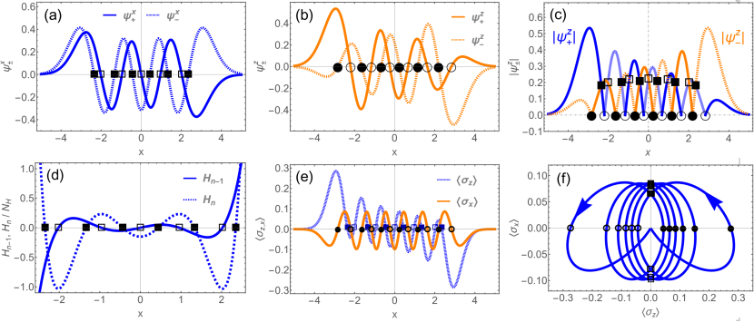
Figure 1: Analytical correspondence of nodes or zeros in wave function components (a-c), Hermite polynomials (d) and spin windings (e,f). The filled (empty) squares mark the corresponding nodes in $\psi^{x}_{+}$ ($\psi^{x}_{-}$), $\langle\sigma_{z}\left(x\right)\rangle$ with positive (negative) $\langle\sigma_{x}\left(x\right)\rangle$, $H_{n}$ ($H_{n-1}$) respectively, while dots (circles) denote the nodes in $\psi^{z}_{+}$ ($\psi^{z}_{-}$), $\langle\sigma_{x}\left(x\right)\rangle$ with positive (negative) $\langle\sigma_{z}\left(x\right)\rangle$. Nodes of $\psi^{x}_{\pm}$ ($\psi^{z}_{\pm}$) are also the amplitude-crossing points $|\psi^{z}_{+}|=|\psi^{z}_{-}|$ ($|\psi^{x}_{+}|=|\psi^{x}_{-}|$) as in (c). Here $\omega=0.5\Omega$, $g=1.5g_{{\rm s}}$, $\lambda=0.2$, $j_{E}=5$ and $g_{\rm s}=\sqrt{\omega\Omega}/2$.

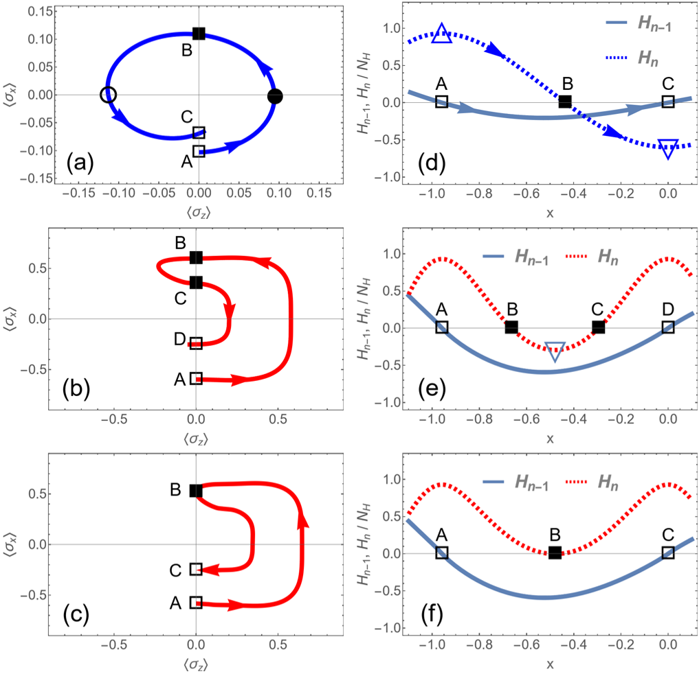
Figure 2: Full winding without anti-winding nodes. (a-c) Schematic spin winding between two adjacent nodes (empty squares) on negative $\langle\sigma_{x}(x)\rangle$ axis, respectively without anti-winding nodes (a), with two anti-winding nodes (filled squares) on positive $\langle\sigma_{x}(x)\rangle$ axis (b), and with one anti-winding nodes (c). (d-f) Required evolution of Hermite polynomial $H_{n}(x)$ (dotted lines) for two adjacent roots (empty squares) in $H_{n-1}(x)$, corresponding to (a-c), with (d) fulfilled and (e,f) unfulfilled.

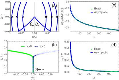
Figure 3: Vanishing external spin-winding angle at infinity. (a) A zoom-in plot of the spin winding in Fig.1(f) around the origin. $\theta_{e}$ is the external winding angle at large $x$. (b) $\theta_{e}$ versus $\langle\sigma_{x}(x)\rangle$ in $|x|\rightarrow\infty$ limit. (c,d) $\log_{10}(\langle\sigma_{z}(x)\rangle/\langle\sigma_{x}(x)\rangle)$ (c) and $\theta_{e}$ (d) versus large $x$ by exact solution (dots) and asymptotic expression (35) (solid line).

IV Topological-transition nature at finite frequencies

IV.1 Wave-function nodes

We can rewrite the eigen wave function in position space

$$\psi_{+}^{x}\left(x\right) \equiv \psi_{n,\Uparrow}^{\left(x,\eta\right)}\left(x\right)=C_{n\Uparrow}^{\left(\eta\right)}\phi_{n-1}\left(x\right)/\sqrt{N_{n}},$$ (14)

$$\psi_{-}^{x}\left(x\right) \equiv \psi_{n,\Downarrow}^{\left(x,\eta\right)}\left(x\right)=C_{n\Downarrow}^{\left(\eta\right)}\phi_{n}\left(x\right)/\sqrt{N_{n}}.$$ (15)

where $\phi_{n}\left(x\right)$ is the eigenstate of quantum harmonic oscillator with quantum number $n$

$$\phi_{n}\left(x\right)=\frac{1}{\pi^{1/4}\sqrt{2^{n}n!}}H_{n}\left(x\right)e^{-x^{2}/2}.$$ (16)

Note the Hermite polynomial $H_{n}\left(x\right)$ has an $n$ number of real roots, $x=y_{{\rm Z}}$ where $H_{n}\left(y_{{\rm Z}}\right)=0,$ accordingly the wave function components $\psi_{n,\Uparrow}^{\left(x,\eta\right)}\left(x\right)$ and $\psi_{n,\Downarrow}^{\left(x,\eta\right)}\left(x\right)$ respectively have $n-1$ and $n$ numbers of real nodes $y_{{\rm Z}}$ where $\psi_{n,\sigma_{x}}^{\left(x,\pm\right)}\left(y_{{\rm Z}}\right)=0$.

We can also transform onto the spin-$\sigma_{z}$ basis, represented by $\uparrow$ and $\downarrow$, on which the wave function becomes

$$\psi_{n}^{\left(z,\eta\right)}=\ \psi_{+}^{z}\left(x\right)\left|\uparrow\right\rangle+\psi_{-}^{z}\left(x\right)\left|\downarrow\right\rangle$$ (17)

with spin components

$$\psi_{+}^{z}\left(x\right) \equiv \psi_{n,\uparrow}^{\left(z,\eta\right)}\left(x\right)=\frac{C_{n\Uparrow}^{\left(\eta\right)}\phi_{n-1}\left(x\right)+C_{n\Downarrow}^{\left(\eta\right)}\phi_{n}\left(x\right)}{\sqrt{2N_{n}}},$$ (18)

$$\psi_{-}^{z}\left(x\right) \equiv \psi_{n,\downarrow}^{\left(z,\eta\right)}\left(x\right)=\frac{C_{n\Uparrow}^{\left(\eta\right)}\phi_{n-1}\left(x\right)-C_{n\Downarrow}^{\left(\eta\right)}\phi_{n}\left(x\right)}{\sqrt{2N_{n}}}.$$ (19)

The parity symmetry ensures

$$\psi_{n,\uparrow}^{\left(z,\eta\right)}\left(x\right)=\left(-1\right)^{n-1}\psi_{n,\downarrow}^{\left(z,\eta\right)}\left(-x\right).$$ (20)

Later on in Sect. IV.4 we will see that both components have $n$ number of nodes, $x=x_{{\rm Z}}$, where $\psi_{n,\sigma_{z}}^{\left(z,\eta\right)}\left(x_{{\rm Z}}\right)=0.$

We give an example of eigen wave function in Fig. 1 (a-c) for $n=6$ with $\psi_{\pm}^{x,z}\left(x\right)\$representing $\psi_{n,\sigma_{x}}^{\left(x,\eta\right)}\left(x\right)$ and $\psi_{n,\sigma_{z}}^{\left(z,\eta\right)}\left(x\right)$ in Eqs. (14,15,18,19). Here in the figure the nodes of $\psi_{\pm}^{x}\left(x\right)$ are marked by empty boxes (spin-up, $+=\Uparrow$) and filled boxes (spin-down, $-=\Downarrow$) in panel (a), and the nodes of $\psi_{\pm}^{z}\left(x\right)$ by circles (spin-up, $+=\uparrow$) and dots (spin-down, $-=\downarrow$) in panel (b). We can also plot all the nodes together in the wave-function amplitude $\left|\psi_{\pm}^{z}\left(x\right)\right|$ as in panel (c) where the nodes of $\psi_{n,\sigma_{x}}^{\left(x,\eta\right)}\left(x\right)$ are located at points $\left|\psi_{+}^{z}\left(x\right)\right|=\left|\psi_{-}^{z}\left(x\right)\right|$. Here the empty boxes ($\Uparrow$) are crossing points of $\psi_{+}^{z}\left(x\right)=\psi_{-}^{z}\left(x\right)$ in both solid lines ($\psi_{\pm}^{z}>0$) or both broken lines ($\psi_{\pm}^{z}<0$), while filled boxes ($\Downarrow$) are crossing points of $\psi_{+}^{z}\left(x\right)=-\psi_{-}^{z}\left(x\right)$ between solid lines and broken lines.

The node number represents the topological structure of the wave function in the sense that with a fixed node number one cannot go to another node state by continuous shape deformation of the wave function, just as one cannot change a torus into a sphere by a continuous deformation in the topological picture of so-called rubber-sheet geometry. Such wave-function topological structure can be reflected by physical topological character as there is a one-to-one correspondence between the wave-function nodes and the spin-winding nodes, as we shall discuss in the following sections.

IV.2 Spin winding: Node correspondence to wave function and symmetric/anti-symmetric properties

Note the eigen wave functions in (7) and (8) are real, so that the corresponding spin texture are related to the wave function components by

$$\langle\sigma_{z}\left(x\right)\rangle = \psi_{+}^{z}\left(x\right)^{2}-\psi_{-}^{z}\left(x\right)^{2}=2\psi_{+}^{x}\left(x\right)\psi_{-}^{x}\left(x\right)$$ (21)

$$\langle\sigma_{x}\left(x\right)\rangle = \psi_{+}^{x}\left(x\right)^{2}-\psi_{-}^{x}\left(x\right)^{2}=2\psi_{+}^{z}\left(x\right)\psi_{-}^{z}\left(x\right),$$ (22)

$$\langle\sigma_{y}\left(x\right)\rangle = i\left[\psi_{-}^{z}\left(x\right)^{\ast}\psi_{+}^{z}\left(x\right)-\psi_{+}^{z}\left(x\right)^{\ast}\psi_{-}^{z}\left(x\right)\right]=0.$$ (23)

We see the spin are winding within $\langle\sigma_{z}\left(x\right)\rangle$-$\langle\sigma_{z}\left(x\right)\rangle$ plane, and the nodes of eigen wave function are in one-to-one correspondence to the nodes of the spin winding:

$$\psi_{n,\sigma_{z}}^{\left(z,\eta\right)}\left(x_{{\rm Z}}\right) = 0\Longleftrightarrow\langle\sigma_{z}\left(x_{{\rm Z}}\right)\rangle=0,$$ (24)

$$\psi_{n,\sigma_{x}}^{\left(x,\eta\right)}\left(y_{{\rm Z}}\right) = 0\Longleftrightarrow\langle\sigma_{x}\left(y_{{\rm Z}}\right)\rangle=0.$$ (25)

The node correspondence of the wave function and the spin winding is shown by panels (a-c) and (e,f) in Fig. 1, where the squares represent the corresponding nodes of $\psi^{x}_{\pm}$ and $\langle\sigma_{z}\left(x\right)\rangle$ and the dots or circles locate the corresponding nodes of $\psi^{z}_{\pm}$ and $\langle\sigma_{x}\left(x\right)\rangle$.

From Eqs. (21-23) the spin texture for state $\psi_{n}^{\left(x,\eta\right)}$ can be analytically obtained to be

$$\langle\sigma_{z}\left(x\right)\rangle=\frac{e^{-x^{2}}g\ C_{n\omega\eta}}{2^{n-3/2}N_{\sigma}}H_{n-1}\left(x\right)H_{n}\left(x\right),$$ (26)

$$\langle\sigma_{x}\left(x\right)\rangle=\frac{e^{-x^{2}}}{2^{n}N_{\sigma}}[C_{n\omega\eta}^{2}H_{n-1}\left(x\right)^{2}-2g^{2}H_{n}\left(x\right)^{2}],$$ (27)

$$\langle\sigma_{y}\left(x\right)\rangle=0,$$ (28)

where $N_{\sigma}=\sqrt{\pi}(n-1)!\ [4g^{2}n+C_{n\omega\eta}\Omega_{n\omega\chi}]$, $C_{n\omega\eta}=\Omega_{n\omega\chi}+\eta\sqrt{\Omega_{n\omega\chi}^{2}+4g^{2}n}$, $\Omega_{n\omega\chi}=[\Omega-\omega+\left(2n-1\right)\chi\omega]$. For state $\psi_{0}$, we have $\langle\sigma_{z}\left(x\right)\rangle=\langle\sigma_{y}\left(x\right)\rangle=0$ and $\langle\sigma_{x}\left(x\right)\rangle=-e^{-x^{2}}/\sqrt{\pi}$. Eqs. (26) and (27) indicate that there is also a correspondence of the roots of the Hermite polynomials to the nodes of the wave function and the spin winding, as illustrated by Fig. 1(d). We will leave more discussions around Eq. (30) in Sect. IV.3 and with $f_{\pm}$ in Sect. IV.4.

The parity symmetry also leads to the symmetry of $\langle\sigma_{x}\left(x\right)\rangle$ and anti-symmetry of $\langle\sigma_{z}\left(x\right)\rangle$. Indeed, the parity symmetry implies $\psi_{-}^{z}\left(x\right)=P\psi_{+}^{z}\left(-x\right)$ Ying2020-nonlinear-bias , substitution of which into (21) and (22) yields

$$\langle\sigma_{z}\left(-x\right)\rangle=-\langle\sigma_{z}\left(x\right)\rangle,\quad\langle\sigma_{x}\left(-x\right)\rangle=+\langle\sigma_{x}\left(x\right)\rangle.$$ (29)

The above symmetric and anti-symmetric properties of $\langle\sigma_{x}\left(x\right)\rangle$ and $\langle\sigma_{z}\left(x\right)\rangle$ can also be directly seen from (26) and (27) as $H_{n}\left(-x\right)=\left(-1\right)^{n}H_{n}\left(x\right)$. Fig. 1(e) shows an example of the spin texture, one sees that indeed $\langle\sigma_{x}\left(x\right)\rangle$ is symmetric and $\langle\sigma_{z}\left(x\right)\rangle$ is anti-symmetric, which yields a $\langle\sigma_{z}\left(x\right)\rangle$-reflection-symmetric spin winding in the $\langle\sigma_{z}\left(x\right)\rangle$-$\langle\sigma_{x}\left(x\right)\rangle$ plane as demonstrated in Fig. 1(f). These symmetry properties of the spin texture will be used in the argument for the distribution of $\langle\sigma_{x}\left(x\right)\rangle$ nodes.

IV.3 Invariant $\langle\sigma_{z}\left(x\right)\rangle$ nodes

From Eq. (26) we see the nodes of $\langle\sigma_{z}\left(x\right)\rangle$ are completely decided by the roots of $H_{n-1}\left(x\right)$ and $H_{n}\left(x\right)$. The $\langle\sigma_{z}\left(x\right)\rangle$ nodes are located at the roots of the Hermite polynomials

$$H_{n-1}(z_{{\rm Z}}^{\left(n-1\right)})=0,\text{ or }H_{n}(z_{{\rm Z}}^{\left(n\right)})=0,$$ (30)

which are independent of the model parameters. Such an invariant feature may provide some particular advantage in designing potential topological devices. For an example, these spin nodes could provide a topological information for quantum topological encoding and decoding Ying-Spin-Winding , the topological information based on such a kind of invariant nodes will be robust as it is completely unaffected by the variations of the parameters within the topological phase.

IV.4 Full winding without anti-winding nodes

It should be noted that the Hermite-polynomial roots $z_{{\rm Z}}^{\left(n-1\right)},z_{{\rm Z}}^{\left(n\right)}$ are alternate due to the relation

$$H_{n}^{\prime}\left(x\right)\equiv\partial_{x}H_{n}\left(x\right)=2nH_{n-1}\left(x\right)$$ (31)

which indicates that the $H_{n-1}$ roots, $z_{Z}^{\left(n-1\right)},$ are always the maxima or minima of $H_{n}\left(x\right)$, as shown by the upward and downward triangles in Fig. 2(d). And from relation $H_{n}\left(x\right)=2xH_{n-1}\left(x\right)-\partial_{x}H_{n-1}\left(x\right)$ we see

$$H_{n}(z_{{\rm Z}}^{\left(n-1\right)})=-H_{n-1}^{\prime}(z_{{\rm Z}}^{\left(n-1\right)})$$ (32)

which indicates that two adjacent roots $z_{Z,j}^{\left(n-1\right)},z_{Z,j+1}^{\left(n-1\right)}$ must have different signs of $H_{n}$ due to the different gradient signs from $H_{n-1}^{\prime}$, i.e.

$$H_{n}(z_{{\rm Z},j}^{\left(n-1\right)})H_{n}(z_{{\rm Z},j+1}^{\left(n-1\right)})<0,$$ (33)

leading to a root $z_{Z}^{\left(n\right)}$ between $z_{Z,j}^{\left(n-1\right)}$ and $z_{Z,j+1}^{\left(n-1\right)}$ (Note here $H_{n}(z_{{\rm Z},j}^{\left(n-1\right)})$, $H_{n}(z_{{\rm Z},j+1}^{\left(n-1\right)})$ are always finite due to the Turán inequality $H_{n}\left(x\right)^{2}-H_{n-1}\left(x\right)H_{n+1}\left(x\right)>0$ which excludes simultaneous zeros of $H_{n}\left(x\right)$ and $H_{n-1}\left(x\right)$). Fig. 2(b) shows such a case schematically: the empty boxes A and C represent the two adjacent $H_{n-1}$ roots, at which the gradient has different signs as indicated by the arrow orientations along the solid line. The $H_{n}$ signs at A and C are different (indicated by the triangles) which must surround an $H_{n}$ root (filled square B).

Note from Eqs. (26) and (27) we find $H_{n-1}$ roots and $H_{n}$ roots correspond to $\langle\sigma_{z}\left(x\right)\rangle$ nodes on opposite $\langle\sigma_{x}\left(x\right)\rangle$ axes, as in Fig. 2(a). Thus, the above analysis means that between two adjacent $\langle\sigma_{z}\left(x\right)\rangle$ nodes on same $\langle\sigma_{x}\left(x\right)\rangle$ axis (empty squares A,C) there must be another $\langle\sigma_{z}\left(x\right)\rangle$ node on the opposite $\langle\sigma_{x}\left(x\right)\rangle$ axis (filled square B). The possibility to have more than one $\langle\sigma_{z}\left(x\right)\rangle$ nodes on the opposite $\langle\sigma_{x}\left(x\right)\rangle$ axis as in Fig. 2(b) is excluded, as that would spuriously bring some new $H_{n}$ maximum or minimum which however has no match of $H_{n-1}$ zero, violating relation (31), as denoted by the triangle in Fig. 2(e). This excluded case in Fig. 2(b) also avoids anti-winding (i.e. cancelation of spin-winding angle in route returning). The anti-winding at one $\langle\sigma_{z}\left(x\right)\rangle$ node as in Fig. 2(c) is also violating relation (31). Therefore, the $\sigma_{z}\left(x\right)\rangle$ nodes should appear alternately on positive and negative $\langle\sigma_{x}\left(x\right)\rangle$ axes without anti-winding.

The same happens for $\langle\sigma_{x}\left(x\right)\rangle$ nodes. Actually Eq. (27) can be factorized into a product of factors $f_{\pm}=H_{n-1}\left(x\right)\pm cH_{n}\left(x\right)$ where $c$ is parameter-decided coefficient. The $\langle\sigma_{x}\left(x\right)\rangle$ nodes are just the $f_{\pm}$ roots. Both factors $f_{\pm}$ have $n$ roots as $H_{n-1}\left(x\right)$ and $H_{n}\left(x\right)$ subject to relation (31) are interlacing with alternate zeros as in Fig. 1(d), while the number of the $f_{\pm}$ roots is decided by the crossing times of $H_{n-1}\left(x\right)$ and $H_{n}\left(x\right)$ which are unaffected by any amplitude amplification with nonzero $c$, as one can recognize from Fig. 2(d). Thus, there are $2n$ of $\langle\sigma_{x}\left(x\right)\rangle$ nodes, while from the Eq. (27) we have known there are $2n-1$ of $\langle\sigma_{z}\left(x\right)\rangle$ nodes. Since there is no anti-winding, the $\langle\sigma_{x}\left(x\right)\rangle$ nodes and the $\langle\sigma_{z}\left(x\right)\rangle$ nodes are also interlacing. Indeed, except the node on the infinity side, each $\langle\sigma_{x}\left(x\right)\rangle$ node can only appear in the interval between two adjacent $\langle\sigma_{z}\left(x\right)\rangle$ nodes on opposite $\langle\sigma_{x}\left(x\right)\rangle$ axes, while each interval can accommodate one and only one $\langle\sigma_{x}\left(x\right)\rangle$ node, otherwise accommodation of more $\langle\sigma_{x}\left(x\right)\rangle$ nodes would totally outnumber the $2n$ number of $\langle\sigma_{x}\left(x\right)\rangle$ nodes due to the $\langle\sigma_{z}\left(x\right)\rangle$-reflection-symmetry afore-mentioned at (29).

Wrapping up the above analysis points one rigorously comes to the conclusion that the spin is in full winding without anti-winding nodes, the nodes come in counterclockwise sequence 1234 as in Fig. 2(a) or clockwise sequence 1432 on: (1) positive-$\langle\sigma_{z}\left(x\right)\rangle$ axis (dot), (2) positive-$\langle\sigma_{x}\left(x\right)\rangle$ axis (filled square), (3) negative-$\langle\sigma_{z}\left(x\right)\rangle$ axis (dot), (4) negative-$\langle\sigma_{x}\left(x\right)\rangle$ axis (empty square), periodically till completing the total spin winding at infinity. Such clarification of the full winding behavior is necessary for the explicit extraction of the winding number later on in Sect. IV.6.

IV.5 Spurious fractional winding angle at infinity

Apart from the main part of spin winding in the node sequence, the total winding angle is also partially decided by the winding at infinity. A focus plot on the external winding angle $\theta_{e}$ is illustrated in Fig. 3(a). At a first glance one might think $\theta_{e}$ is fractionally finite. However a more careful tracking of $\theta_{e}$ at larger $\left|x\right|$ reveals that $\theta_{e}$ is approaching to zero at infinity, as shown in Fig. 3(b). Indeed, at infinity the leading term of Hermite polynomials is

$$H_{n}\left(x\right)\rightarrow\left(2x\right)^{n},$$ (34)

so that we have the ratio of the spin texture

$$\frac{\langle\sigma_{z}\left(x\right)\rangle}{\langle\sigma_{x}\left(x\right)\rangle}\rightarrow-\frac{\Omega_{n\omega\chi}+\eta\sqrt{4g^{2}n+\Omega_{n\omega\chi}^{2}}}{\sqrt{2}g}\frac{1}{x},$$ (35)

which is approaching to zero. As demonstrated in Fig. 3(c), this asymptotic behavior (solid line) agrees well with the exact ratio (dots) obtained by Eqs. (26) and (27). Correspondingly, as shown in Fig. 3(d), the external angle of spin winding is vanishing at infinity

$$\theta_{\infty}=\arctan\frac{\langle\sigma_{z}\left(x\right)\rangle}{\langle\sigma_{x}\left(x\right)\rangle}\rightarrow 0.$$ (36)

This vanishing external angle achieves an integer number of total spin winding angle as formulated in next section.

IV.6 Winding number in terms of nodes

One can know the rounds of spin winding by the winding number around the origin in the $\langle\sigma_{z}\rangle$-$\langle\sigma_{x}\rangle$ plane as calculated by

$$n_{zx}=\frac{1}{2\pi}\int_{-\infty}^{\infty}\frac{\langle\sigma_{z}\left(x\right)\rangle\partial_{x}\langle\sigma_{x}\left(x\right)\rangle-\langle\sigma_{x}\left(x\right)\rangle\partial_{x}\langle\sigma_{z}\left(x\right)\rangle}{\langle\sigma_{z}\left(x\right)\rangle^{2}+\langle\sigma_{x}\left(x\right)\rangle^{2}}dx,$$ (37)

which has also been applied in topological classification in nanowire systems and quantum systems with geometric driving Ying2016Ellipse ; Ying2017EllipseSC ; Ying2020PRR ; Gentile2022NatElec . With the normalized spin texture

$$\langle\overline{\sigma}_{z,x}\left(x\right)\rangle=\frac{\langle\sigma_{z,x}\left(x\right)\rangle}{\sqrt{\langle\sigma_{z}\left(x\right)\rangle^{2}+\langle\sigma_{x}\left(x\right)\rangle^{2}}},$$ (38)

we can rewrite the integrand to be

$$\frac{\langle\sigma_{z}\left(x\right)\rangle\partial_{x}\langle\sigma_{x}\left(x\right)\rangle-\langle\sigma_{x}\left(x\right)\rangle\partial_{x}\langle\sigma_{z}\left(x\right)\rangle}{\langle\sigma_{z}\left(x\right)\rangle^{2}+\langle\sigma_{x}\left(x\right)\rangle^{2}}$$ (39)

$$= \frac{-\partial_{x}\langle\overline{\sigma}_{z}\left(x\right)\rangle}{\eta_{x}\sqrt{1-\langle\overline{\sigma}_{z}\left(x\right)\rangle^{2}}}=\frac{\partial_{x}\langle\overline{\sigma}_{x}\left(x\right)\rangle}{\eta_{z}\sqrt{1-\langle\overline{\sigma}_{x}\left(x\right)\rangle^{2}}},$$

where $\eta_{x,z}={\rm sign}\langle\overline{\sigma}_{x,z}\left(x\right)\rangle$, so that the integral (37) can be worked out explicitly in terms of either $\langle\sigma_{x}\left(x\right)\rangle$ or $\langle\sigma_{z}\left(x\right)\rangle$ nodes

$$n_{zx} = -\sum_{i=0}^{M_{x}}\frac{\arcsin\langle\overline{\sigma}_{z}\left(x_{Z,i+1}\right)\rangle-\arcsin\langle\overline{\sigma}_{z}\left(x_{Z,i}\right)\rangle}{2\pi\eta_{x}\left(i\right)}$$ (40)

$$= \sum_{i=1}^{M_{z}}\frac{\arcsin\langle\overline{\sigma}_{x}\left(y_{Z,i+1}\right)\rangle-\arcsin\langle\overline{\sigma}_{x}\left(y_{Z,i}\right)\rangle}{2\pi\eta_{z}\left(i\right)}.$$ (41)

Attention should be paid here that the summation in Eq.(40) (Eq. (41)) is respectively over the $M_{x}$ number of $\langle\sigma_{x}\left(x\right)\rangle$ nodes (the $M_{z}$ number of $\langle\sigma_{z}\left(x\right)\rangle$ nodes), i.e. over $x_{Z,i}$ ($y_{Z,i}$), not over the nodes of the variable $\langle\sigma_{z}\left(x\right)\rangle$ ($\langle\sigma_{x}\left(x\right)\rangle$) in the integrand (39). Corresponding to $\eta_{x,z}$ in (39), $\eta_{x}\left(i\right)$ ($\eta_{z}\left(i\right)$) is the sign of $\langle\sigma_{x}\left(x\right)\rangle$ ($\langle\sigma_{z}\left(x\right)\rangle$) in space section $x\in(x_{Z,i},x_{Z,i+1})$ ($x\in(y_{Z,i},y_{Z,i+1})$), which can be represented by the sign of a $\langle\sigma_{z}\left(x\right)\rangle$ node ($\langle\sigma_{x}\left(x\right)\rangle$ node) in the section. The edge sections $i=0,M_{x,z}$ are $(-\infty,x_{Z,1})$ and $(x_{Z,M_{x}},\infty)$ ($(-\infty,y_{Z,1})$ and $(y_{Z,M_{z}},\infty)$). We have set $x_{Z,0}=-\infty$ and $x_{Z,M_{x}+1}=\infty$ ($y_{Z,0}=-\infty$ and $y_{Z,M_{z}+1}=\infty$).

Note $\arcsin\langle\overline{\sigma}_{z}\left(y_{Z,i}\right)\rangle=\frac{\pi}{2}{\rm sign}[\overline{\sigma}_{z}\left(y_{Z,i}\right)]$ and $\arcsin\langle\overline{\sigma}_{x}\left(x_{Z,i}\right)\rangle=\frac{\pi}{2}{\rm sign}[\overline{\sigma}_{x}\left(x_{Z,i}\right)]$, we arrive at

$$n_{zx} = -\sum_{i=0}^{M_{x}}\frac{sgn\langle\overline{\sigma}_{z}\left(x_{Z,i+1}\right)\rangle-sgn\langle\overline{\sigma}_{z}\left(x_{Z,i}\right)\rangle}{4\eta_{x}\left(i\right)}$$ (42)

$$= \sum_{i=0}^{M_{z}}\frac{sgn\langle\overline{\sigma}_{x}\left(y_{Z,i+1}\right)\rangle-sgn\langle\overline{\sigma}_{x}\left(y_{Z,i}\right)\rangle}{4\eta_{z}\left(i\right)}$$ (43)

where we have set the function $sgn(\overline{\sigma}_{x,z})={\rm sign}(\overline{\sigma}_{x,z})$ for the nodes and $sgn(\overline{\sigma}_{x,z})=2\arcsin(\overline{\sigma}_{x,z})/\pi$ for the infinity ends. Finally only the neighboring nodes with opposite signs have contributions.

Expressions (40)-(42) are valid for general spin windings. Note the original version of winding number (37) involves calculus of both integral and differential, which is numerically more difficult to treat. In contrast, Eqs. (42) and (42) are simple algebraic expressions comprising only a finite number of nodes of $\langle\sigma_{z}\left(x\right)\rangle$ and $\langle\sigma_{x}\left(x\right)\rangle$, which much simplifies the calculation of the winding number. Moreover, the integral (37) depends on the topological structure of the spin texture geometrically, the equivalence of Eqs. (42) and (42) to Eq. (37) indicates that, given the few points of nodes, the topological winding number remains the same no matter how the spin texture is geometrically deformed, which reclaims the original sense of topological classification in the so-called rubber-sheet geometry. As Eqs. (42) and (42) are the nodes the order of which encodes the topological message by an algebraic code as in the end of Sect. IV.4, it is also a demonstration of bridging of the geometrical topology and the algebraic topology, here physically in context of wave function and spin winding.

According to the discussions in Sections IV.4 and IV.5, the spin is in full winding without anti-winding nodes and the external winding angle at infinity is vanishing. Note there are $M_{x}=2n$ of $\langle\sigma_{x}\left(x\right)\rangle$ nodes and $M_{z}=2n-1$ of $\langle\sigma_{z}\left(x\right)\rangle$ nodes, while the infinity ends only contribute to $sgn(\overline{\sigma}_{z})$ to complete a full integer rounds of winding. Thus, from (40) and (41) we can readily conclude that the magnitude of spin winding number is

$$\left|n_{{\rm w}}\right|=\left|n_{zx}\right|=n.$$ (44)

The sign of $n_{{\rm w}}$ is decided by the winding direction, which is reflected in $\eta_{x,z}\left(i\right)$ and can be more explicitly obtained by the status at infinity as in the following.

IV.7 Winding direction

Since the winding is smooth without anti-winding nodes and the external winding angle is zero at infinity, $\theta_{\infty}\rightarrow 0$, the winding direction can be determined by the signs of $\langle\sigma_{z}\left(x\right)\rangle$ and $\langle\sigma_{x}\left(x\right)\rangle$ at infinity where the spin winding starts and ends. The winding will be counter-clockwise if $\langle\sigma_{z}\left(x\right)\rangle$ starts to grow negatively (positively) while $\langle\sigma_{x}\left(x\right)\rangle$ increases positively (negatively), which happens in the 2nd (4th) quadrant; Otherwise the winding is clockwise if $\langle\sigma_{z}\left(x\right)\rangle$ and $\langle\sigma_{x}\left(x\right)\rangle$ start in the 1st (3rd) quadrant. Clockwise winding starting in the 2nd (4th) quadrant or counter-clockwise winding starting in the 1st (3rd) quadrant is excluded as that would lead to $M_{z}=2n+1>M_{x}=2n$ which conflicts with the afore-discussed node numbers determined by Eqs.(26) and (27). Thus, the winding is counter-clockwise (clockwise) if the sign

$$s_{{\rm w}} = \text{sign}\frac{\langle\sigma_{z}\left(x\right)\rangle}{\langle\sigma_{x}\left(x\right)\rangle}|_{x\rightarrow-\infty}$$ (45)

$$= \text{sign}\left[\Omega_{n\omega\chi}+\eta\sqrt{4g^{2}n+\Omega_{n\omega\chi}^{2}}\right]$$

is negative (positive). This indicates that all states with $\eta=-1$ have a counter-clockwise spin winding direction, while the winding direction of the states with $\eta=+1$ is opposite. The ground state is composed of $\eta=-1$ states thus has a counter-clockwise winding direction.

Thus, the energy branch label $\eta$ and the excitation number $n$ together give the complete information of the spin winding number for state $\psi_{n}^{\left(x,\eta\right)}$,

$$n_{{\rm w}}=s_{{\rm w}}n=-\eta n,$$ (46)

which is the topological quantum number. Now we see that both $\eta$ and $n$ are endowed topological connotations, respectively representing the winding direction and the magnitude of winding number.

IV.8 Topological phase diagram

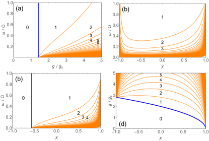
Figure 4: Topological phase diagrams. Ground-state spin winding number $n_{{\rm w}}$ in $g$-$\omega$ plane at $\chi=0.5$ (a), $\chi$-$\omega$ plane for $g=2.5g_{{\rm s}}$ (b) and $g=3.0g_{{\rm s}}$ (b) at $\chi=0.5$, and $\chi$-$g$ plane at $\omega=0.3\Omega$ (d).

To have an overall view of all the phase transitions, we show the ground-state phase diagrams in $g$-$\omega$, $\chi$-$\omega$, and $\chi$-$g$ planes by Fig. 4 where the numbers mark $n_{{\rm w}}$. The phase boundaries shifting states from $\psi_{n}^{(x,-1)}$ to $\psi_{n+1}^{(x,-1)}$ can be analytically obtained for $n=0$

$$g_{c}^{(0,1)}=2g_{\rm s}\sqrt{1-\chi},$$ (47)

and for $n>0$

$$g_{c}^{(n,n+1)}=2g_{\rm s}\sqrt{\left(\chi_{+}+2n\chi_{+}\chi_{-}\right)\widetilde{\omega}-\chi+S_{r}},$$ (48)

where $S_{r}=\sqrt{(1-\chi_{+}\widetilde{\omega})^{2}+4n(n+1)\chi_{+}\chi_{-}\widetilde{\omega}^{2}}$, $\widetilde{\omega}=\omega/\Omega$, $\chi_{\pm}=1\pm\chi$, and $g_{\rm s}=\sqrt{\omega\Omega}/2$. Here in the figure the blue (thick) line represents the principal boundary $g_{c}^{(0,1)}$ where the first transition occurs from $n_{{\rm w}}=0$ phase to $n_{{\rm w}}=1$ phase when the coupling $g$ is increasing at a fixed Stark coupling $\chi$ in panel (a) or when $\chi$ is increasing at a fixed $g$ in panel (b). The principal boundary disappears if the fixed $g$ is larger than $g_{c}^{(0,1)}$ as in panel (c), which can be seen more clearly in panel (d) where $g_{c}^{(0,1)}$ exists in a finite range within the physical regime $\chi\in[-1,1]$. Here one finds that the critical couplings can be tuned by $\chi$.

V Simultaneous occurrence of Landau-class and topological-class transitions

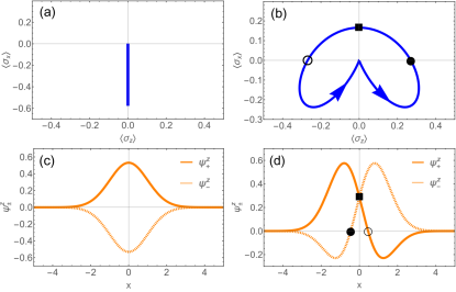
Figure 5: Simultaneous occurrence of symmetry-protected topological class of transition and symmetry-breaking Landau class of transition. (a,b) Ground-state spin profile in $\langle\sigma_{z}\left(x\right)\rangle$-$\langle\sigma_{x}\left(x\right)\rangle$ plane in $n_{{\rm w}}=0$ phase (a) and $n_{{\rm w}}=1$ phase (b). (c,d) Ground-state wave function $\psi_{\pm}^{z}(x)$ with $\hat{P}_{x}$ and $\hat{P}_{\sigma}$ symmetries in $n_{{\rm w}}=0$ phase (c) and broken $\hat{P}_{x}$ and $\hat{P}_{\sigma}$ symmetries in $n_{{\rm w}}=1$ phase (d). Here $g=0.8g_{{\rm s}}$ (a,c) and $g=2.0g_{{\rm s}}$ (b,d) at $\omega=0.6\Omega$, $\chi=0.5$.

As mentioned in Introduction, the Landau class of transitions break the symmetry while the topological class of transitions preserve the symmetry. Conventionally these two classes of transitions are incompatible due to the contrary symmetry requirements. However, here the principal transition at $g_{c}^{(0,1)}$ provides a paradigmatic case of exception, as it turns out to be both Landau class of transition and topological class of transition simultaneously.

V.1 Topological-class transition feature at $g_{c}^{(0,1)}$: Transition of spin winding topology

As addressed in the previous section, we have seen the topological nature of all the transitions, including the principal transition at $g_{c}^{(0,1)}$. To have a direct feeling of the topological transtion for the principal transition, in Fig. 5(a,b) we plot spin profiles in $\langle\sigma_{z}\left(x\right)\rangle$-$\langle\sigma_{z}\left(x\right)\rangle$ plane for the phases before and after the transition. As one can see, in the $n_{{\rm w}}=0$ phase the spin profile is completely flat ($\langle\sigma_{z}\left(x\right)\rangle=0$ $\forall x$) and does not wind at all as in panel (a), while in the $n_{{\rm w}}=1$ phase the spin is winding non-trivially as in panel (b). These two totally different spin widing styles provide a sharp topological contrast for recognization of the topological nature of transition.

V.2 Landau-class transition feature at $g_{c}^{(0,1)}$: Symmetry breaking of space inversion and spin reversion

The $n_{{\rm w}}=0$ phase before the principal transition at $g_{c}^{(0,1)}$ is also special as it posseses more symmteries than the Hamiltonian. Indeed, besides the parity symmetry, the state $\psi_{0}=\left|0,\Downarrow\right\rangle$ in this phase has symmetries of space inversion and spin reversion:

$$\hat{P}_{x}\psi_{0}=\psi_{0},\qquad\hat{P}_{\sigma}\psi_{0}=-\psi_{0},$$ (49)

where

$$\hat{P}_{x}=\left(-1\right)^{a^{\dagger}a},\qquad\hat{P}_{\sigma}=\sigma_{x}.$$ (50)

In the position space on the $\sigma_{z}$ basis the wave function takes the form $\psi_{0}=\psi_{0,+}^{z}\left(x\right)\left|\uparrow\right\rangle+\psi_{0,-}^{z}\left(x\right)\left|\downarrow\right\rangle=\left[\phi_{0}\left(x\right)\left|\uparrow\right\rangle-\phi_{0}\left(x\right)\left|\downarrow\right\rangle\right]/\sqrt{2}$ where $\phi_{0}\left(x\right)$ is the Gaussian function. The symmetry operator $\hat{P}_{x}$ actually inverses the space Ying2020-nonlinear-bias of a function $\hat{P}_{x}F\left(x\right)=F\left(-x\right)$ which gives

$$\hat{P}_{x}\psi_{0}\left(x\right) = \psi_{0}\left(x\right),$$ (51)

$$\hat{P}_{\sigma}\psi_{0}\left(x\right) = -\psi_{0}\left(x\right),$$ (52)

as $\phi_{0}\left(x\right)$ is an even function. The space inversion and spin reversion are more directly visible from the plot of the wave function components in Fig. 5(c). It should be mentioned that theses symmetries in Eqs. (17)-(20) are rigorously fulfilled at any finite frequencies, in contrast to the QRM and the anisotropic QRM where the low-frequency condition is required for the validity of these symmetries Ying-2021-AQT . The unlimited frequency condition greatly relaxes the experimental requirements for QPTs Ying2015 .

On the contrary, in other phases with $n_{{\rm w}}\neq 0$, the symmetries of space inversion and spin reversion are broken. Ineed, from Eqs. (17)-(20) one can easily recognize

$$\hat{P}_{x}\psi_{n}^{\left(z,\eta\right)}\left(x\right) \neq \pm\psi_{n}^{\left(z,\eta\right)}\left(x\right),$$ (53)

$$\hat{P}_{\sigma}\psi_{n}^{\left(z,\eta\right)}\left(x\right) \neq \pm\psi_{n}^{\left(z,\eta\right)}\left(x\right),$$ (54)

in contrast to the symmetry-preserving Eqs. (51) and (52). In Fig. 5(d) with $n_{{\rm w}}=1$ one sees directly that the wave function is asymmetric under either space inversion or spin reversion.

Thus, the principal transition from state $\psi_{0}$ to state $\psi_{1}^{\left(z,\eta\right)}$ is accompanied with the symmetry breaking of both space inversion and spin reversion. This symmetry breaking feature holds without approximation at any frequencies. In such a symmetry-breaking sense, the the principal transition also belongs to the Landau class of transition. Also, in the Landau theory the energy is expressed as a functional of some order parameters. We leave the discussion in terms of variational energy as a functional of the order parameters in symmetry breaking around the transition in Appendix A.

V.3 Key for reconciliation of the two contrary transition classes: Unbroken higher symmetry

We have seen at $g_{c}^{(0,1)}$ the simultaneous occurrence of the topological class of transition and the Landau class of transition which are conventionally incompatible due to opposite symmetry requirements. The key for their simultaneous occurrence or coexistence essentially lies in the reconcilable situation that the symmetry which the topological class of transition preserves is actually different from the symmetries which the Landau class of transition breaks. Indeed, the symmetry that protects the topological feature of the spin winding for the eigenstates in the transitions is the parity symmetry $\hat{P}$, which comprises both the space inversion and the spin reversal

$$\hat{P}=\hat{P}_{x}\hat{P}_{\sigma}.$$ (55)

As mentioned in Sect. II, the $g_{y}$ term in the coupling is effectively the Rashba spin-orbit coupling or equal-weight mixture of the linear Dresselhaus and Rashba spin-orbit couplings Ying-2021-AQT ; Ying-gapped-top ; Ying-Stark-top ; Ying-Spin-Winding , which involves the spin nontrivially and drives the spin winding. The parity symmetry guarantees the symmetric spin texture in (29) and its connection at the two infinity ends in the position variation, which establishes the symmetry situation for the TPTs. Note both before and after the transition $g_{c}^{(0,1)}$ this parity symmetry that atcually protects all the TPTs is still preserved

$$\hat{P}\psi_{0}\left(x\right) = -\psi_{0}\left(x\right),$$ (56)

$$\hat{P}\psi_{n}^{\left(z,\eta\right)}\left(x\right) = \pm\psi_{n}^{\left(z,\eta\right)}\left(x\right),$$ (57)

even when the subsymmetries in the space inversion and the spin reversal are both broken. Therefore, the conventionally opposite symmetry requirements for the Landau class and topological class of phase transitions reconcile each other here and we see the simultaneous occurrence or coexistence of the two contrary transition classes.

VI Understanding unconventional topological transitions in the presence of counter-rotating term

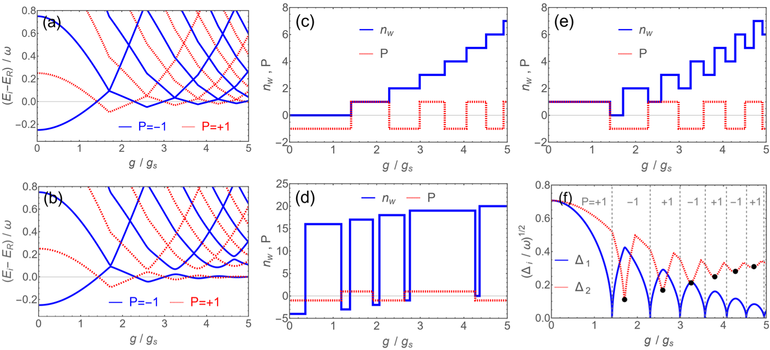
Figure 6: Topological transitions without parity variation and origin for unconventional topological transitions without gap closing. (a,b) Energy spectrum $E_{i}-E_{R}$ in the absence ((a), $\lambda=0$) and in the presence ((b), $\lambda=0.01$) of the counter-rotating term, with the reference energy $E_{R}=(E_{2}+E_{1})/2$. (c,d,e) Spin winding number $n_{{\rm w}}$ (blue solid) and parity $P$ (red dotted) for $j_{E}=1$ (c), $j_{E}=20$ (d), and $j_{E}=2$ (e) at $\lambda=0$. (f) The first and second excitation gap $\Delta_{i}=E_{i+1}-E_{i}$ at $\lambda=0.01$. The dots in (f) are results by Eq. (60). Here in all panels $\omega=0.3\Omega$ and $\chi=0.5$.

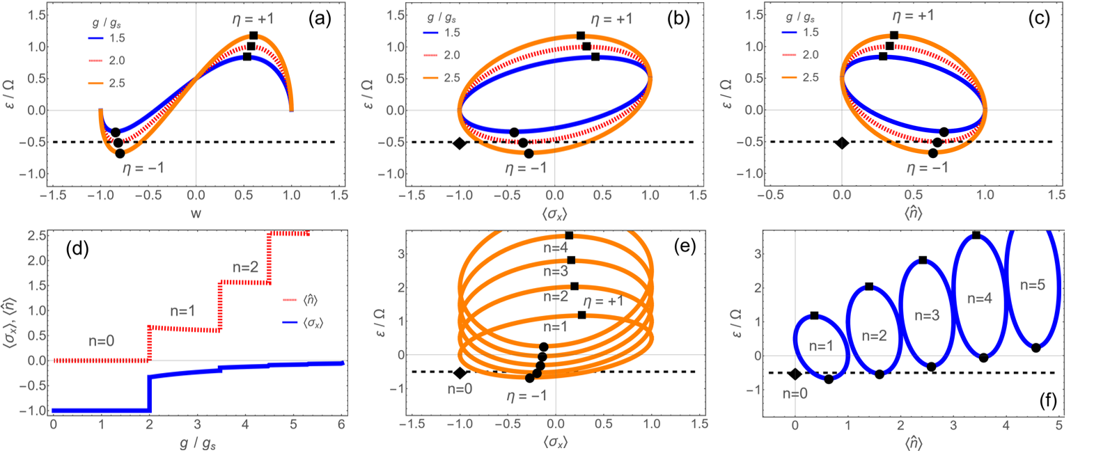
Figure 7: Variational energy $\varepsilon$ as a functional of order parameters in symmetry breaking. (a-c) $\varepsilon$ as a functional of $w$ (a), $\langle\sigma_{x}\rangle$ (b), $\langle\hat{n}\rangle$ (c) for state $\psi_{1}$ before ($g=1.5g_{{\rm s}}$, orange (light) solid line), at ($g=2.0g_{{\rm s}}$, dotted line) and after ($g=2.5g_{{\rm s}}$, blue solid (dark) line) the transition $g_{c}^{(0,1)}$ in competition with the energy of state $\psi_{0}$ (thin dashed line). (d) $\langle\sigma_{x}\rangle$ (solid) and $\langle\hat{n}\rangle$ (dotted) versus $g$ for the ground state. (e,f) $\varepsilon$ as a function of $\langle\sigma_{x}\rangle$ (e) or $\langle\hat{n}\rangle$ (f) for states $\psi_{n}$ at $g=2.5g_{{\rm s}}$. The dots mark the minimized energy and the squares label the maximized energy, which reproduces the exact JC energy in $\eta=-1$ and $\eta=+1$ branches, while the diamond locates the order parameters for $\psi_{0}$. State $\psi_{0}$ (diamond) preserves the subsymmetries $\hat{P}_{x}$ and $\hat{P}_{\sigma}$ as indicated by integer numbers of $\langle\sigma_{x}\rangle$ and $\langle\hat{n}\rangle$, while the other states (dots and squares) break the subsymmetries as reflected by deviations of $\langle\sigma_{x}\rangle$ from $\pm 1$ and $\langle\hat{n}\rangle$ from integer numbers. Here $\omega=0.5\Omega$, $\lambda=0$, $\chi=0$ in all panels.

Most TPTs in the anisotropic QRM are conventional ones Ying-2021-AQT which occur with gap closing as those in condensed matter Topo-Wen ; Hasan2010-RMP-topo ; Yu2010ScienceHall ; Chen2019GapClosing ; TopCriterion ; Top-Guan ; TopNori . Unconventional TPTs without gap closing also exist Ying-gapped-top ; Ying-Stark-top analogously to the unconventional cases in the quantum spin Hall effect with strong electron-electron interactions Amaricci-2015-no-gap-closing and the quantum anomalous Hall effect with disorder Xie-QAH-2021 . These unconventional TPTs lie in the ground state by a mechanism of node introduction from the infinity Ying-gapped-top ; Ying-Stark-top . On the other hand, it is found that unconventional TPTs emerge more frequently in excited states, especially around level anti-crossings Ying-Spin-Winding . Here from the JC-Stark model we can gain some insight for the origin of such unconventional TPTs in excited states.

In Fig. 6 panel (a) shows the energy spectrum of the JC-Stark model, where levels are crossing among the all states with negative parity (blue solid) and positive parity (red dotted). Panel (b) gives the spin winding number $n_{w}$ (solid line) of the ground state ($j_{E}=1$) which jumps always at parity variation (dotted line) and gap closing (similar to the solid line in panel (f)). The spin winding can turn direction in excited states, as indicated by the negative values of $n_{w}$ in panel (d) for state $j_{E}=20$ according to the discussion in Sect. IV.7. Each jump of $n_{w}$ is accompanied with a TPT. In particular, some TPTs occur without parity variation, as illustrated in panel (e) for state $j_{E}=2,$ which comes from the level crossing between same parity states. Note here the gap is sill closing at the transitions despite no parity variation. What interesting is, once we add anisotropy, e.g. $\lambda=0.01$, the gap at these TPTs opens, as demonstrated by the energy spectrum by panel (b) and more clearly by the dotted line in panel (f). This gap opening accounts for the afore-mentioned unconventional TPTs in the excited.

A clearer explanation can be given by regarding the counter-rotating term as a perturbation around these transitions which mainly involves the two level-crossing states $\psi_{n}^{\left(x,\eta\right)},\psi_{n^{\prime}}^{\left(x,\eta^{\prime}\right)}$ with energies $\varepsilon_{1}=E^{\left(n,\eta\right)}$, $\varepsilon_{2}=E^{\left(n^{\prime},\eta^{\prime}\right)}$ and winding numbers $n_{w,1}=-\eta n$, $n_{w,2}=-\eta^{\prime}n^{\prime}$. On the basis of these two states the Hamiltonian in matrix form can be written as

$$H\approx\left(\begin{array}[]{cc}E^{\left(n,\eta\right)}&d\\ d&E^{\left(n^{\prime},\eta^{\prime}\right)}\end{array}\right)$$ (58)

where

$$d=\langle\psi_{n}|H_{\lambda}|\psi_{n^{\prime}}\rangle = \lambda g\sqrt{n^{\prime}+1}\frac{C_{n\Uparrow}^{\left(\eta\right)}C_{n^{\prime}\Downarrow}^{\left(\eta^{\prime}\right)}}{\sqrt{N_{n}N_{n^{\prime}}}}\delta_{n,n^{\prime}+2}$$ (59)

$$+\lambda g\sqrt{n^{\prime}-1}\frac{C_{n\Downarrow}^{\left(\eta\right)}C_{n^{\prime}\Uparrow}^{\left(\eta^{\prime}\right)}}{\sqrt{N_{n}N_{n^{\prime}}}}\delta_{n,n^{\prime}-2}$$

and $H_{\lambda}$ is the counter-rotating term in (3) beyond the JC-Stark model. The crossing levels are split as $E_{\pm}=\frac{1}{2}(E^{\left(n,\eta\right)}+E^{\left(n^{\prime},\eta^{\prime}\right)}\pm\Delta)$ with a gap opening at the level-crossing point $E^{\left(n,\eta\right)}=E^{\left(n^{\prime},\eta^{\prime}\right)},$

$$\Delta=\sqrt{(E^{\left(n,\eta\right)}-E^{\left(n^{\prime},\eta^{\prime}\right)})^{2}+4d^{2}}\rightarrow 2|d|,$$ (60)

which is finite for $n=n^{\prime}\pm 2$, leading to the level anti-crossing. The validity of Eq. (60) is confirmed by the dots which match well the numerical result by exact diagonalization Ying2020-nonlinear-bias ; Ying-Spin-Winding in the dotted line in Fig. 6(f). Here from Eqs. (59) and (60) one sees that the gap opening does not occur for crossing states with different parity, since they respectively have even and odd $n$ as indicated by $P=\left(-1\right)^{n}$ from Eq. (9). Note the small $\lambda$ here is a perturbation which is not yet enough to change the winding numbers so that $n_{w}$ remains similar to $\lambda=0$ case in Fig. 6(e). Thus, the TPTs originally at level crossing now become unconventional TPTs without gap closing as the gap is opening. Larger $\lambda$ may induce more unconventional TPTs than those inherited from the $\lambda=0$ case at the gap opening Ying-Spin-Winding . Finally it should be noticed that such unconventional TPTs are still protected by the parity symmetry as the added term $H_{\lambda}$ preserves the parity symmetry, $[H_{\lambda},\hat{P}]=0$. The above analysis provides a simple but clear understanding for the unconventional TPTs in excited states.

VII Conclusions and Discussions

We have presented a rigorous study to show the topological nature of transitions in Jaynes-Cummings Model generally with Stark non-linear Coupling, which is a fundamental model for light-matter interactions. The exact and explicit solution of the model enables us to analytically analyze the nodes of eigen wave functions and establish the exact correspondence to the nodes in the spin texture. In the light of the Hermite polynomial properties, we have proven that the spin nodes on $\langle\sigma_{z}\left(x\right)\rangle$ and $\langle\sigma_{x}\left(x\right)\rangle$ axes are interlacing on positive and negative axes, thus the node sequence forms a smooth spin winding without anti-winding nodes. In particular, the spurious fractional winding angle at infinity is found to be integer, which achieves a full winding. Thus, the phase transitions in the model have a nature of TPTs.

Based on a strict derivation we have reformulated the spin winding number to facilitate the extraction of winding numbers by replacing the integral formula with an algebraic formula in terms of finite points of nodes, which also bridges the geometrical topology and the algebraic topology in a physical way. The excitation number and the energy branch label of eigen states turn out to the magnitude and the sign (winding direction) of the winding number, thus both endowed a topological connotation unrecognized before.

In particular, we have found that the $\langle\sigma_{x}\left(x\right)\rangle$ nodes are invariant, which might have potential advantage in designing topological devices as they provide robust topological information unaffected by variations of the parameters.

We have also demonstrated that the principal transition has the character of Landau class of phase transition besides that of TPT, by pointing out the symmetry breaking aspect and variational energy analysis as functional of order parameters. Note conventionally Landau class of phase transitions and topological class of phase transitions are incompatible due to the contrary symmetry requirements, here the principal transition establishes a paradigmatic case that a transition can be both symmetry-breaking Landau class of transition and symmetry-protected topological class of transition simultaneously. The key for the reconciliation of the two contradictory classes of transitions lies in the preserved higher symmetry which protects the TPTs despite the subsymmetries are broken in the Landau class of transition.

Moreover, we have applied our result to analyze the gap opening at some particular TPTs without parity variations in the presence of the counter-rotating term, which gives an analytical explanation for the unconventional TPTs without gap closing. Note that a gapped situation can avoid the detrimental time divergent problem in preparing sensing state Ying2022-Metrology , the unconventional TPTs may similarly have potential advantages in possible applications or designing quantum topological devices. In such a favorable situation, our understanding might be helpful for further exploring and exploiting unconventional TPTs in light-matter interactions.

Finally it is worthwhile to mention that the model considered in the present work may be implemented in realistic systems, e.g. in superconducting circuits. Indeed, both the anisotropy PRX-Xie-Anistropy ; Forn-Diaz2010 ; Pietikainen2017 ; Yimin2018 ; Wang2019Anisotropy and the Stark nonlinear coupling Stark-Grimsmo2013 ; Stark-Grimsmo2014 ; Stark-Cong2020 are adjustable. Besides realizations of ultra-strong couplings in $\lambda\neq 0$ case Diaz2019RevModPhy ; Wallraff2004 ; Gunter2009 ; Niemczyk2010 ; Peropadre2010 ; FornDiaz2017 ; Forn-Diaz2010 ; Scalari2012 ; Xiang2013 ; Yoshihara2017NatPhys ; Kockum2017 ; Bayer2017DeepStrong , access to ultra-strong couplings can be also possible for $\lambda=0$ Ulstrong-JC-1 ; Ulstrong-JC-3-Adam-2019 ; Ulstrong-JC-2 . The position $x$ can be represented by the flux of Josephson junctions and the spin texture might be measured by interference devices and magnetometer you024532 . These systems may provide platforms for possible tests or applications of our results. Our analysis might be also relevant for some other systems as the effective Rashba/Dresselhaus spin-orbit coupling in our model shares similarity with those in nanowires Nagasawa2013Rings ; Ying2016Ellipse ; Ying2017EllipseSC ; Ying2020PRR ; Gentile2022NatElec , cold atoms Li2012PRL ; LinRashbaBECExp2011 and relativistic systems Bermudez2007 .

Appendix A Variational energy as functional of order parameters

In this appendix we present some discussions in terms of energy functional of order parameters in the situation of the symmetry breaking at the principal transition. Although the exact solution has been obtained in Sec. III, a reformulation for energy as a functional of order parameters is more connected with the Landau theory of phase transitions. Under the constraint of the $U(1)$ symmetry the eigenstate of the JC-Stark model should be either a linear combination of bases $\left|n-1,\Uparrow\right\rangle$ and $\left|n,\Downarrow\right\rangle$

$$\psi_{n}=\sqrt{1-w^{2}}\left|n-1,\Uparrow\right\rangle+w\left|n,\Downarrow\right\rangle$$ (61)

or composed solely of $\psi_{0}=\left|0,\Downarrow\right\rangle.$ The energy of $\psi_{0}$ is simply $E^{0}=-\Omega/2$, while the energy of $\psi_{n}$ is variational with respect to the basis weight $w$:

$$\varepsilon=\varepsilon_{0}+\left[\omega-\Omega-\chi\omega\left(2n-1\right)\right]w^{2}+2\sqrt{n}g\sqrt{1-w^{2}}w.$$ (62)

where $\varepsilon_{0}=\left(1+\chi\right)\omega\left(n-1\right)+\frac{\Omega}{2}$ is independent of $w$. The minimization and maximization of $\varepsilon$ with respect to $w$ lead to

$$w_{\pm}=\pm\sqrt{\frac{4g^{2}n+A_{w}^{2}\pm A_{w}\sqrt{4g^{2}n+A_{w}^{2}}}{8g^{2}n+2A_{w}^{2}}},$$ (63)

where $A_{w}=[(2n-1)\chi-1]\omega+\Omega,$ which is equivalent YingVarM to (10)(11) with $\eta=\pm$.

Note the relations

$$\langle\hat{n}\rangle = n-1+w^{2},$$ (64)

$$\langle\sigma_{x}\rangle = \left(1-2w^{2}\right),$$ (65)

the variational energy can be rewritten into a functional of the order parameter $\langle\sigma_{x}\rangle$ or $\langle\hat{n}\rangle$

$$\varepsilon = \varepsilon_{0}-C_{\varepsilon}\left(1-\langle\sigma_{x}\rangle\right)+\eta\sqrt{n}g\sqrt{1-\langle\sigma_{x}\rangle^{2}}$$ (66)

$$\varepsilon = \varepsilon_{0}-2C_{\varepsilon}\left(\langle\hat{n}\rangle+1-n\right)$$ (67)

$$+\eta 2\sqrt{n}g\sqrt{\left(n-\langle\hat{n}\rangle\right)\left(\langle\hat{n}\rangle+1-n\right)}$$

where $C_{\varepsilon}=\left[\frac{\Omega-\omega}{2}+\left(n-\frac{1}{2}\right)\chi\omega\right]$. Fig. 7 illustrates some examples of the variational energy around the transition at $g_{c}^{(0,1)}$ in competition to the energy of $\psi_{0}$. The dots mark the minimized energy while the squares label the maximized energy. One sees that when $g$ is increasing, the minimized energy becomes lower than that of state $\psi_{0}$, which triggers a first-order transition unlike the second-order transition in the QRM or the anisotropic QRM Ying2020-nonlinear-bias ; Ying-Stark-top in the low frequency limit. The upper branch ($\eta=+1$) and the lower branch ($\eta=-1$) of the variational energy $\varepsilon$ are connected and form energy circles as shown in panel (d), the lowest and highest points are the final energies, which together with $E^{0}$ reproduce the exact energies in Eq. (12) not only for the ground state but also for the excited states as demonstrated in panels (e) and (f).

Note the energy and the order parameters of $\psi_{0}$ are represented by the diamonds in Fig. 7(b,c,d,e), where the expectation value $\langle\sigma_{x}\rangle=\langle\hat{P}_{x}\rangle=-1$ implies the spin reversal symmetry in (51) and $\langle\hat{n}\rangle=0$ indicates the space inversion symmetry in (52). As a contrast, the values of $\langle\sigma_{x}\rangle$ and $\langle\hat{n}\rangle$ for the minimum and maximum points on the energy circles deviate from the integer numbers, which means breaking of these symmetries.

References

- (1) D. Braak, Phys. Rev. Lett. 107, 100401 (2011).
- (2) E. Solano, Physics 4, 68 (2011).
- (3) See a review of theoretical methods for light-matter interactions in A. Le Boité, Adv. Quantum Technol. 3, 1900140 (2020).
- (4) See a review of quantum phase transitions in light-matter interactions e.g. in J. Liu, M. Liu, Z.-J. Ying, and H.-G. Luo, Adv. Quantum Technol. 4, 2000139 (2021).
- (5) P. Forn-Díaz, L. Lamata, E. Rico, J. Kono, and E. Solano, Rev. Mod. Phys. 91, 025005 (2019).
- (6) A. F. Kockum, A. Miranowicz, S. De Liberato, S. Savasta, and F. Nori, Nature Reviews Physics 1, 19 (2019).
- (7) Z.-L. Xiang, S. Ashhab, J. Q. You, and F. Nori, Rev. Mod. Phys. 85, 623 (2013). J. Q. You and F. Nori, Phys. Rev. B 68, 064509, (2003).
- (8) A. Wallraff, D. I. Schuster, A. Blais, L. Frunzio, R.-S. Huang, J. Majer, S. Kumar, S. M. Girvin, and R. J. Schoelkopf, Nature 431, 162 (2004).
- (9) C. Ciuti, G. Bastard, and I. Carusotto, Phys. Rev. B 72, 115303 (2005).
- (10) A. A. Anappara, S. De Liberato, A. Tredicucci, C. Ciuti, G. Biasiol, L. Sorba, and F. Beltram, Phys. Rev. B 79, 201303(R) (2009).
- (11) G. Günter, A. A. Anappara, J. Hees, A. Sell, G. Biasiol, L. Sorba, S. De Liberato, C. Ciuti, A. Tredicucci, A. Leitenstorfer, and R. Huber, Nature 458, 178 (2009).
- (12) P. Forn-Díaz, J. Lisenfeld, D. Marcos, J. J. Garcia-Ripoll, E. Solano, C. J. P. M. Harmans, and J. E. Mooij, Phys. Rev. Lett. 105, 237001 (2010).
- (13) T. Niemczyk, F. Deppe, H. Huebl, E. P. Menzel, F. Hocke, M. J. Schwarz, J. J. Garcia-Ripoll, D. Zueco, T. Hümmer, E. Solano, A. Marx, and R. Gross, Nature Phys. 6, 772 (2010).
- (14) B. Peropadre, P. Forn-Díaz, E. Solano, and J. J. García-Ripoll, Phys. Rev. Lett. 105, 023601 (2010).
- (15) G. Scalari, C. Maissen, D. Turčinková, D. Hagenmüller, S. De Liberato, C. Ciuti, C. Reichl, D. Schuh, W. Wegscheider, M. Beck, and J. Faist, Science 335, 1323 (2012).
- (16) P. Forn-Díaz, J. J. García-Ripoll, B. Peropadre, J. L. Orgiazzi, M. A. Yurtalan, R. Belyansky, C. M. Wilson, and A. Lupascu, Nat. Phys. 13, 39 (2017).
- (17) X. Gu, A. F. Kockum, A. Miranowicz, Y. X. Liu, and F. Nori, Phys. Rep. 718-719, 1 (2017).
- (18) F. Yoshihara, T. Fuse, S. Ashhab, K. Kakuyanagi, S. Saito, and K. Semba, Nat. Phys. 13, 44 (2017).
- (19) A. Bayer, M. Pozimski, S. Schambeck, D. Schuh, R. Huber, D. Bougeard, and C. Lange, Nano Lett. 17, 6340 (2017).
- (20) S. Ashhab, Phys. Rev. A 87, 013826 (2013).
- (21) Z.-J. Ying, M. Liu, H.-G. Luo, H.-Q.Lin, and J. Q. You, Phys. Rev. A 92, 053823 (2015).
- (22) M.-J. Hwang, R. Puebla, and M. B. Plenio, Phys. Rev. Lett. 115, 180404 (2015).
- (23) M.-J. Hwang and M. B. Plenio, Phys. Rev. Lett. 117, 123602 (2016).
- (24) J. Larson and E. K. Irish, J. Phys. A: Math. Theor. 50, 174002 (2017).
- (25) M. Liu, S. Chesi, Z.-J. Ying, X. Chen, H.-G. Luo, and H.-Q. Lin, Phys. Rev. Lett. 119, 220601 (2017).
- (26) Z.-J. Ying, L. Cong, and X.-M. Sun, arXiv:1804.08128, 2018; J. Phys. A: Math. Theor. 53, 345301 (2020).
- (27) Z.-J. Ying, Phys. Rev. A 103, 063701 (2021).
- (28) Z.-J. Ying, Adv. Quantum Technol. 5, 2100088 (2022); ibid. 5, 2270013 (2022).
- (29) Z.-J. Ying, Adv. Quantum Technol. 5, 2100165 (2022).
- (30) Z.-J. Ying, Adv. Quantum Technol. 6, 2200068 (2023); ibid. 6, 2370011 (2023).
- (31) Z.-J. Ying, Adv. Quantum Technol. 6, 2200177 (2023); ibid. 6, 2370071 (2023).
- (32) R. Grimaudo, A. S. Magalhães de Castro, A. Messina, E. Solano, and D. Valenti, Phys. Rev. Lett. 130, 043602 (2023).
- (33) R. Grimaudo, D. Valenti, A. Sergi, and A. Messina, Entropy 25, 187 (2023).
- (34) F. A. Wolf, M. Kollar, and D. Braak, Phys. Rev. A 85, 053817 (2012).
- (35) S. Felicetti and A. Le Boité, Phys. Rev. Lett. 124, 040404 (2020).
- (36) S. Felicetti, M.-J. Hwang, and A. Le Boité, Phy. Rev. A 98, 053859 (2018).
- (37) U. Alushi, T. Ramos, J. J. García-Ripoll, R. Di Candia, and S. Felicetti, PRX Quantum 4, 030326 (2023).
- (38) E. K. Irish and A. D. Armour, Phys. Rev. Lett. 129, 183603 (2022).
- (39) E. K. Irish and J. Gea-Banacloche, Phys. Rev. B 89, 085421 (2014).
- (40) D. Braak, Q.H. Chen, M.T. Batchelor, and E. Solano, J. Phys. A Math. Theor. 49, 300301 (2016).
- (41) A. J. Maciejewski, M. Przybylska, and T. Stachowiak, Phys. Lett. A 378, 3445 (2014); Phys. Lett. A 379, 1503 (2015).
- (42) H. P. Eckle and H. Johannesson, J. Phys. A: Math. Theor. 50, 294004 (2017).
- (43) Y.-F. Xie, L. Duan, Q.-H. Chen, J. Phys. A: Math. Theor. 52, 245304 (2019).
- (44) Y.-Q. Shi, L. Cong, and H.-P. Eckle, Phys. Rev. A 105, 062450 (2022).
- (45) Q.-T. Xie, S. Cui, J.-P. Cao, L. Amico, and H. Fan, Phys. Rev. X 4, 021046 (2014).
- (46) S. Felicetti, D. Z. Rossatto, E. Rico, E. Solano, and P. Forn-Díaz, Phys. Rev. A 97, 013851 (2018).
- (47) S. Felicetti, J. S. Pedernales, I. L. Egusquiza, G. Romero, L. Lamata, D. Braak, E. Solano, Phys. Rev. A 92, 033817 (2015).
- (48) L. Garbe, I. L. Egusquiza, E. Solano, C. Ciuti, T. Coudreau, P. Milman, S. Felicetti, Phys. Rev. A 95, 053854 (2017).
- (49) R. J. Armenta Rico, F. H. Maldonado-Villamizar, and B. M. Rodriguez-Lara, Phys. Rev. A 101, 063825 (2020).
- (50) L. Garbe, M. Bina, A. Keller, M. G. A. Paris, and S. Felicetti, Phys. Rev. Lett. 124, 120504 (2020).
- (51) L. Garbe, O. Abah, S. Felicetti, and R. Puebla, Phys. Rev. Research 4, 043061 (2022).
- (52) T. Ilias, D. Yang, S. F. Huelga, M. B. Plenio, PRX Quantum 3, 010354 (2022).
- (53) Z.-J. Ying, S. Felicetti, G. Liu, D. Braak, Entropy 24, 1015 (2022).
- (54) A. Le Boité, M.-J. Hwang, H. Nha, and M. B. Plenio, Phys. Rev. A 94, 033827 (2016).
- (55) A. Ridolfo, M. Leib, S. Savasta, and M. J. Hartmann, Phys. Rev. Lett. 109, 193602 (2012).
- (56) Z.-M. Li, D. Ferri, D. Tilbrook, and M. T. Batchelor, J. Phys. A: Math. Theor. 54, 405201 (2021).
- (57) M. Liu, Z.-J. Ying, J.-H. An, and H.-G. Luo, New J. Phys. 17, 043001 (2015).
- (58) L. Cong, X.-M. Sun, M. Liu, Z.-J. Ying, H.-G. Luo, Phys. Rev. A 95, 063803 (2017).
- (59) L. Cong, X.-M. Sun, M. Liu, Z.-J. Ying, H.-G. Luo, Phys. Rev. A 99, 013815 (2019).
- (60) G. Liu, W. Xiong, and Z.-J. Ying, arXiv:2302.07163, to appear in Phys. Rev. A, (2023).
- (61) K. K. W. Ma, Phys. Rev. A 102, 053709 (2020).
- (62) Q.-H. Chen, C. Wang, S. He, T. Liu, and K.-L. Wang, Phys. Rev. A 86, 023822 (2012).
- (63) L. Duan, Y.-F. Xie, D. Braak, Q.-H. Chen, J. Phys. A 49, 464002 (2016).
- (64) Y.-Y. Zhang, Phys. Rev. A 94, 063824 (2016).
- (65) Z. Lü, C. Zhao, and H. Zheng, J. Phys. A: Math. Theor. 50, 074002 (2017).
- (66) L.-T. Shen, Z.-B. Yang, H.-Z. Wu, and S.-B. Zheng, Phys. Rev. A 95, 013819 (2017).
- (67) Y. Yan, Z. Lü, L. Chen, and H. Zheng, Adv. Quantum Technol. 6, 2200191 (2023).
- (68) X. Chen, Z. Wu, M. Jiang, X.-Y. Lü, X. Peng, and J. Du, Nat. Commun. 12, 6281 (2021).
- (69) X. Y. Lü, L. L. Zheng, G. L. Zhu, and Y. Wu, Phys. Rev. Applied 9, 064006 (2018).
- (70) B.-L. You, X.-Y. Liu, S.-J. Cheng, C. Wang, and X.-L. Gao, Acta Phys. Sin. 70 100201 (2021).
- (71) M. T. Batchelor and H.-Q. Zhou, Phys. Rev. A 91, 053808 (2015).
- (72) Q. Xie, H. Zhong, M. T. Batchelor, and C. Lee, J. Phys. A: Math. Theor. 50, 113001 (2017).
- (73) S. Bera, S. Florens, H. U. Baranger, N. Roch, A. Nazir, and A. W. Chin, Phys. Rev. B 89, 121108(R) (2014).
- (74) L. Yu, S. Zhu, Q. Liang, G. Chen, and S. Jia, Phys. Rev. A 86, 015803 (2012).
- (75) T. Liu, M. Feng, W. L. Yang, J. H. Zou, L. Li, Y. X. Fan, and K. L. Wang, Phys. Rev. A 88, 013820 (2013).
- (76) J. Peng, E. Rico, J. Zhong, E. Solano, and I. L. Egusquiza, Phys. Rev. A 100, 063820 (2019).
- (77) J. Casanova, R. Puebla, H. Moya-Cessa, and M. B. Plenio, npj Quantum Information 4, 47 (2018).
- (78) D. Braak, Symmetry 11, 1259 (2019).
- (79) V. V. Mangazeev, M. T. Batchelor, and V. V. Bazhanov, J. Phys. A: Math. Theor. 54, 12LT01 (2021).
- (80) Z.-M. Li and M. T. Batchelor, Phys. Rev. A 103, 023719 (2021).
- (81) C. Reyes-Bustos, D. Braak, and M. Wakayama, J. Phys. A: Math. Theor. 54, 285202 (2021).
- (82) J. Larson and T. Mavrogordatos, The Jaynes-Cummings Model and Its Descendants, IOP, London, (2021).
- (83) L. Cong, S. Felicetti, J. Casanova, L. Lamata, E. Solano, and I. Arrazola, Phys. Rev. A 101, 032350 (2020).
- (84) A. L. Grimsmo, and S. Parkins, Phys. Rev. A 87, 033814 (2013).
- (85) A. L. Grimsmo and S. Parkins, Phys. Rev. A 89, 033802 (2014).
- (86) L. D. Landau, Zh. Eksp. Teor. Fiz. 7, 19 (1937).
- (87) D. J. Thouless, M. Kohmoto, M. P. Nightingale, and M. den Nijs, Phys. Rev. Lett. 49, 405 (1982).
- (88) J. M. Kosterlitz, and D. J. Thouless. Journal of Physics C: Solid State Phys. 6, 1181 (1973).
- (89) F. D. M. Haldane, Phys. Lett. A 93, 464 (1983).
- (90) F. D. M. Haldane, Phys. Rev. Lett. 50, 1153 (1983).
- (91) Z.-C. Gu and X.-G. Wen, Phys. Rev. B 80, 155131 (2009).
- (92) X.-G. Wen, Rev. Mod. Phys. 2017, 89, 041004.
- (93) S. Sachdev, Quantum phase transitions, 2nd ed. Cambridge University Press, Cambridge, UK, 2011.
- (94) I. I. Rabi, Phys. Rev. 51, 652 (1937).
- (95) H.-P. Eckle, Models of Quantum Matter, Oxford University Press, UK, 2019.
- (96) M. Z. Hasan and C. L. Kane, Rev. Mod. Phys. 82, 3045 (2010).
- (97) R. Yu, W. Zhang, H.-J. Zhang, S.-C. Zhang, X. Dai, and Z. Fang, Science 329, 61 (2010).
- (98) H. Zou, E. Zhao, X.-W. Guan, and W. V. Liu, Phys. Rev. Lett. 122, 180401 (2019).
- (99) W. Chen and A. P. Schnyder, New J. Phys. 21, 073003 (2019).
- (100) Z.-X. Li, Y. Cao, X. R. Wang, and P. Yan, Phys. Rev. Applied 13, 064058 (2020).
- (101) Y. Che, C. Gneiting, T. Liu, and F. Nori, Phys. Rev. B 102, 134213 (2020).
- (102) A. Amaricci, J. C. Budich, M. Capone, B. Trauzettel, and G. Sangiovanni, Phys. Rev. Lett. 114, 185701 (2015).
- (103) C.-Z. Chen, J. Qi, D.-H. Xu, and X.C. Xie, Sci. China Phys. Mech. Astron. 64, 127211 (2021).
- (104) E. T. Jaynes and F. W. Cummings, Proc. IEEE 51, 89 (1963).
- (105) J. E. Mooij, T. P. Orlando, L. Levitov, L. Tian, and C. H. van der Wal, S. Lloyd, Science 285, 1036 (1999).
- (106) F. Nagasawa, D. Frustaglia, H. Saarikoski, K. Richter, and J. Nitta, Nat. Commun. 4, 2526 (2013).
- (107) Z.-J. Ying, P. Gentile, C. Ortix, and M. Cuoco, Phys. Rev. B 94, 081406(R) (2016).
- (108) Z.-J. Ying, M. Cuoco, C. Ortix, and P. Gentile, Phys. Rev. B 96, 100506(R) (2017).
- (109) Z.-J. Ying, P. Gentile, J. P. Baltanás, D. Frustaglia, C. Ortix, and M. Cuoco, Phys. Rev. Res. 2, 023167 (2020).
- (110) P. Gentile, M. Cuoco, O. M. Volkov, Z.-J. Ying, I. J. Vera-Marun, D. Makarov, and C. Ortix, Nature Electronics 5, 551 (2022).
- (111) Y.-J. Lin, K. Jiménez-García, and I. B. Spielman, Nature 471, 83 (2011).
- (112) V. Galitski and I. B. Spielman, Nature 494, 49 (2013).
- (113) G. Dresselhaus, Phys. Rev. 100, 580 (1955).
- (114) Y. A. Bychkov and E. I. Rashba, J. Phys. C 17, 6039 (1984).
- (115) I. Pietikäinen, S. Danilin, K. S. Kumar, A. Vepsäläinen, D. S. Golubev, J. Tuorila, and G. S. Paraoanu, Phys. Rev. B 96, 020501(R) (2017).
- (116) Y. Wang, W.-L. You, M. Liu, Y.-L. Dong, H.-G. Luo, G. Romero, and J. Q. You, New J. Phys. 20, 053061 (2018).
- (117) G. Wang, R. Xiao, H. Z. Shen, and K. Xue, Sci. Rep. 9, 4569 (2019).
- (118) J. Casanova, G. Romero, I. Lizuain, J. J. García-Ripoll, and E. Solano, Phys. Rev. Lett. 105, 263603 (2010).
- (119) A. Stokes and A. Nazir, Nat. Commun. 10, 499 (2019).
- (120) J.-F. Huang, J.-Q. Liao, and L.-M. Kuang, Phys. Rev. A 101, 043835 (2020).
- (121) J. Q. You, Y. Nakamura, and Franco Nori, Phys. Rev. B 71, 024532 (2005).
- (122) Y. Li, L. P. Pitaevskii, and S. Stringari, Phys. Rev. Lett. 108, 225301 (2012).
- (123) A. Bermudez, M. A. Martin-Delgado, and E. Solano, Phys. Rev. A 76, 041801(R) (2007).
- (124) Z.-J. Ying, arXiv:(2023).