Distilling the essential elements of nuclear binding via neural-network quantum states

Abstract

In pursuing the essential elements of nuclear binding, we compute ground-state properties of atomic nuclei with up to $A=20$ nucleons, using as input a leading order pionless effective field theory Hamiltonian. A variational Monte Carlo method based on a new, highly-expressive, neural-network quantum state ansatz is employed to solve the many-body Schrödinger equation in a systematically improvable fashion. In addition to binding energies and charge radii, we accurately evaluate the magnetic moments of these nuclei, as they reveal the self-emergence of the shell structure, which is not a priori encoded in the neural-network ansatz. To this aim, we introduce a novel computational protocol based on adding an external magnetic field to the nuclear Hamiltonian, which allows the neural network to learn the preferred polarization of the nucleus within the given magnetic field.

Introduction.—

Understanding emerging nuclear properties from the interactions among protons and neutrons is a longstanding challenge of nuclear theory Hergert (2020). To address this complex problem, accurate nuclear Hamiltonians have been constructed either within phenomenological approaches Wiringa et al. (1995); Machleidt (2001) or by leveraging the broken chiral symmetry of QCD Entem and Machleidt (2003); Epelbaum et al. (2005); Gezerlis et al. (2013); Lynn et al. (2016); Epelbaum et al. (2015); Piarulli et al. (2015); Entem et al. (2017); Piarulli et al. (2018). Sophisticated potentials are spin-isospin dependent, typically entail high-momentum components, and involve several fitting parameters, usually determined on light nuclear systems.

Quantum many-body methods solve the Schrödinger equation associated with these Hamiltonians with controlled approximations, leading to remarkable success in computing nuclei across the nuclear chart Barrett et al. (2013); Hagen et al. (2014); Hergert et al. (2016); Carbone et al. (2013); Epelbaum et al. (2011); Carlson et al. (2015); Morris et al. (2018); Hu et al. (2022). However, important questions remain unanswered. For instance, no existing Hamiltonian can simultaneously reproduce with high precision the properties of light nuclear systems, the charge radii of medium-mass nuclei, and the neutron-matter equation of state Binder et al. (2014); Lonardoni et al. (2017); Sammarruca and Millerson (2021); Nosyk et al. (2021); Lovato et al. (2022a).

The quest for distilling the “essential elements of nuclear binding” has arisen from these challenges, seeking the simplest nuclear Hamiltonian yielding binding energies and charge radii across the nuclear chart with few percent errors Lu et al. (2019). Arguments based on the unitary limit, large $N_{c}$, and SU(4) symmetry Kievsky et al. (2018); Lu et al. (2019); Lee et al. (2021); Kievsky et al. (2021) suggest that such a Hamiltonian could be derived within pionless effective field theory ($\not{\pi}$EFT) Bedaque and van Kolck (2002). In Ref. Lu et al. (2019) it was proven that a SU(4)-symmetric Hamiltonian, with a non-local three-body force, can accurately model ground-state properties of several nuclei up to $A=40$ nucleons and neutron matter up to saturation density. Similarly, the leading-order (LO) $\not{\pi}$EFT Hamiltonian “o” developed in Ref. Schiavilla et al. (2021) reproduces reasonably well the binding energies of various closed-shell nuclei and yields a neutron matter equation of state that is remarkably close to realistic Hamiltonians Fore et al. (2023) at low densities.

In this work, we carry out an in-depth assessment of the proposed essential Hamiltonians by computing ground-state properties of nuclei with up to $A=20$ nucleons. In addition to their binding energies and radii, we analyze their magnetic moments, which determine the interactions of nuclei with external magnetic fields and contribute to the hyperfine structure in the electronic spectra of the atom Emery (2006). Owing to the significant difference between the $g$ factors associated with the orbital and spin angular momenta of protons and neutrons, they are an ideal test-bed for nuclear models Bohr and Mottelson (1998).

Variational Monte Carlo (VMC) and Green’s function Monte Carlo (GFMC) calculations of light nuclei carried out with realistic Hamiltonians demonstrated the need for two-body contributions in the electromagnetic currents Marcucci et al. (2008); Pastore et al. (2013). Owing to the exponential growth of the spin-isospin basis Carlson et al. (2015), the GFMC is limited to $A\leq 12$ nuclei. The authors of Ref. Martin et al. (2023) used the auxiliary-field diffusion Monte Carlo (AFDMC) to evaluate magnetic moments of nuclei up to ¹⁷F using chiral-EFT Hamiltonians and consistent currents. However, the AFDMC cannot reach much larger systems, owing to the fermion-sign problem, which is exacerbated by the use of oversimplified variational wave functions Gandolfi et al. (2014).

To overcome these limitations, building on the success of earlier works Keeble and Rios (2020); Adams et al. (2021); Gnech et al. (2022); Yang and Zhao (2022), we solve the nuclear many-body Schrödinger equation in a systematically-improvable fashion using a VMC method based on a neural-network quantum state (NQS) ansatz. The expressivity of the hidden-nucleon NQS, initially developed to model the ground-state wave functions of ³H, ³He, ⁴He, and ¹⁶O Lovato et al. (2022b), and dilute neutron matter Fore et al. (2023), is augmented through neural backflow transformations Luo and Clark (2019). The latter are realized by a simplified version of the permutation-equivariant message-passing neural network (MPNN), recently adopted to compute the homogeneous electron gas Pescia et al. (2023) and cold Fermi gases Kim et al. (2023). To reliably evaluate the nuclear magnetic moments, we introduce a novel computational protocol that allows the NQS to learn the preferred polarization of the nucleus.

Methods.—

We model the interactions among protons and neutrons with the LO $\not{\pi}$EFT Hamiltonian, “o”, developed in Ref. Schiavilla et al. (2021). The nucleon-nucleon potential reproduces the $np$ scattering lengths and effective ranges in the $S/T=0/1$ and $1/0$ channels, and it vanishes in odd partial waves. We assume the electromagnetic component to only include the Coulomb force between finite-size protons. A repulsive three-body force is needed to stabilize the systems with more than two nucleons against the Thomas collapse. AFDMC and VMC-NQS calculations showed that the choice $R_{3}=1.0$ fm for the three-nucleon regulator overbinds ¹⁶O and heavier nuclei Schiavilla et al. (2021); Lovato et al. (2022b). To counter it, we opt for $R_{3}=1.1$ fm, as the extended range introduces additional repulsion in heavier systems.

We introduce $X=\{x_{1}\dots x_{A}\}$ to denote the set of single-particle coordinates $x_{i}=\{\mathbf{r}_{i},s^{z}_{i},t^{z}_{i}\}$, which describe the spatial positions and the z-projection of the spin-isospin degrees of freedom of the $A$ nucleons. The hidden-nucleon wave function Moreno et al. (2022); Lovato et al. (2022b) reads

$$\Psi_{HN}(X)\equiv\text{det}\left[\begin{matrix}\phi_{v}(X)&\phi_{v}(X_{h})\\ \phi_{h}(X)&\phi_{h}(X_{h})\end{matrix}\right]\,,$$ (1)

where, $\phi_{v}$ and $\phi_{h}$ denote the visible and hidden orbitals, while $X$ and $X_{h}$ are the $A$ visible and the $A_{h}$ hidden coordinates. Hence, the dimension of the sub-matrices $\phi_{v}(X)$, $\phi_{v}(X_{h})$, $\phi_{h}(X)$, and $\phi_{h}(X_{h})$ are $A\times A$, $A_{h}\times A$, $A\times A_{h}$, and $A_{h}\times A_{h}$, respectively. As a major departure from Ref. Lovato et al. (2022b), all the above matrices are complex valued, and two separate deep neural networks with differentiable activation functions parametrize the logarithm of their moduli and phases. To respect fermion anti-symmetry, the coordinates of the hidden nucleons $X_{h}$ are permutation-invariant functions of the visible ones. We enforce this symmetry using a Deep-Sets architecture Zaheer et al. (2017); Wagstaff et al. (2019) with logsumexp pooling.

As in recent neutron-matter studies Fore et al. (2023), we improve the flexibility of the ansatz by applying equivariant backflow transformations to pre-process the single-nucleon coordinates and include correlation effects. These transformations are implemented by means of a simplified version of the MPNN employed in Refs. Pescia et al. (2023); Kim et al. (2023)

$$\mathbf{y}_{i}=h\Big{(}\mathbf{x}_{i},\sum_{j}m(\mathbf{x}_{i},\mathbf{x}_{j})\Big{)}\,.$$ (2)

Due to the universality of the hidden-nucleon ansatz, the single, albeit enlarged Slater determinant in Eq.(1) is sufficient for modeling the ground-state wave function of both closed- and open-shell nuclei, regardless of their deformation. This characteristic represents a significant advantage compared to “conventional” quantum Monte Carlo methods, where multiple Slater determinants are required to model open-shell systems Lonardoni et al. (2018); Gandolfi et al. (2020). In stark contrast with the majority of nuclear many-body methods, the shell structure of the nucleus is not directly encoded in the NQS, as the parameters of the network are randomly initialized and no pre-training on a Hartree-Fock wave function is performed. All ground-state properties self-emerge during the training of the network, which is performed by minimizing the variational energy of the system. For this purpose, we employ the stochastic reconfiguration algorithm Sorella (2005) with regularization based on the RMSprop method Lovato et al. (2022b). The expectation value of the Hamiltonian and other quantum-mechanical operators of interest is evaluated stochastically using the Metropolis-Hastings algorithm detailed in the Supplemental Material of Ref. Adams et al. (2021), sampling both the spatial and spin-isospin coordinates of the $A$ nucleon

Results.—

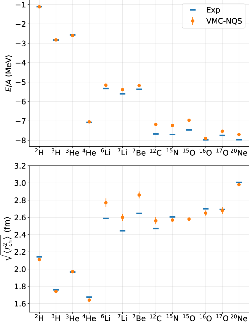
Figure 1: VMC-NQS energy per particle (upper panel) and charge radii (lower panel) of selected nuclei with up to $A=20$ nucleons as obtained from the LO EFT Hamiltonian “o” of Ref. Schiavilla et al. (2021) with $R_{3}=1.1$ fm compared with experimental data.

The upper panel of Fig. 1 displays the ground-state energies per nucleon of selected $A\leq 20$ nuclei obtained solving the ground-state of the $\not{\pi}$EFT Hamiltonian with the VMC-NQS method. The agreement between the computed and experimental values is remarkably good, given the simplicity of the $\not{\pi}$EFT input Hamiltonian. Notably, our ground-state energies are closer to experimental values than those obtained in Ref. Martin et al. (2023) with the AFDMC method and N²LO chiral-EFT interactions. Additionally, we do not observe the increasing overbinding with the number of nucleons reported in no-core shell model calculations that use as input different N²LO two- and three-body forces Maris et al. (2021). Nevertheless, ¹²C and ¹⁵O are under-bound by about $0.6$ MeV per nucleon, while ⁶He, ⁸Li, ⁸B, ⁹C, and ¹⁷F are unstable against breakup into smaller clusters. This behavior suggests an excessive repulsion from the input Hamiltonian, as increasing the flexibility of the NQS by considering more hidden nucleons does not significantly improve the variational energies.

In the lower panel of Fig. 1, we show the charge radii of the same nuclei, which are are derived from the estimates for the point-proton radii taking into account the finite-size of the nucleons and the Darwin-Foldy correction. Here we neglect both the one-body spin-orbit correction of Ref. Ong et al. (2010) and two-body terms in the charge operator Lovato et al. (2013). While the overall trend of experimental data is well reproduced, ²H, ⁴He, and ¹⁶O are slightly smaller than experiments. On the other hand, consistent with the ground-state energies, the radii of ⁶Li, ⁷Li, ⁷Be, and ¹²C are too large — there is no available experimental data for ¹⁵O. In contrast to many-body methods relying on the harmonic-oscillator basis expansion Caprio et al. (2022), the radius converges quickly in our VMC-NQS calculations due to the stability of the method. Hence, the discrepancies between theoretical calculations and experimental data are likely to be ascribed to deficiencies in the input LO $\not{\pi}$EFT Hamiltonian.

At LO in the electroweak current operator, the expectation value of the magnetic moment is given by

$$\mu=\frac{\langle\Psi_{HN}|\sum_{i}P_{i}^{p}L_{i}^{z}+(\mu_{S}+\mu_{V}\tau_{i}^{z})\sigma_{i}^{z}|\Psi_{HN}\rangle}{\langle\Psi_{HN}|\Psi_{HN}\rangle}\,.$$ (3)

In the above equation, $L_{i}^{z}=-i(\mathbf{r}_{i}\times\boldsymbol{\nabla}_{i})_{z}$ is the projection of the orbital angular momentum on the $z$ axis, while $\mu_{S}=0.8798\,\mu_{N}$ and $\mu_{V}=4.0759\,\mu_{N}$, and $\mu_{N}$ is the nuclear magneton. The above definition assumes that the wave function of the nucleus has well defined total angular momentum $J$ and maximal projection on the $z$ axis: $J_{z}=J$. Since the LO $\not{\pi}$EFT Hamiltonian that we employ does not contain tensor or spin-orbit interactions, its ground state is an eigenstate of the total spin $S$ and total orbital angular momentum $L$ and it is degenerate in their projections $S_{z}$ and $L_{z}$: $|\Psi_{HN};L,S\rangle=\sum_{L_{z}S_{z}}c^{L,S}_{L_{z}S_{z}}|L,L_{z};S,S_{z}\rangle$.

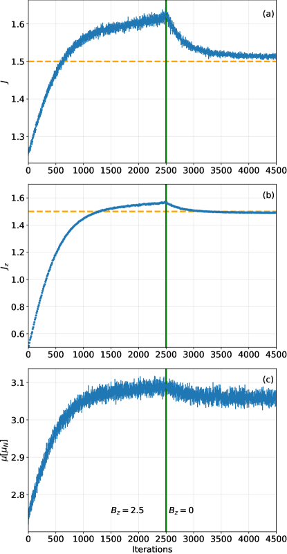
Figure 2: Total angular momentum, its projection on the $z$-axis, and the magnetic moment of ⁷Li while projecting the NQS onto the state with $J,J_{z}=3/2,3/2$. The magnetic field $B_{z}=2.5$ MeV is switched off after 2500 iterations as indicated by the vertical green line. The orange dashed lines represent the target values $J=3/2$ and, $J_{z}=3/2$.

The total polarization of the system $S_{z}$ is conveniently fixed in the Metropolis Hastings Sampling. Hence, since the ground states of ²H, ³H, ³He, and ⁶Li are all $L=0$ (and hence $L_{z}=0$), they are also eigenstates of $J$ and $J_{z}$. On the other hand, evaluating the magnetic moments of heavier nuclei requires projecting the NQS onto a given value of $L_{z}$. To this aim, we have devised a three-stage algorithm. i) A standard SR minimization of the variational energy is carried out to find a good approximation for the nuclear ground state. ii) A small external magnetic field is added to the Hamiltonian, $H\to H-B_{z}L_{z}$, and another energy minimization is carried out to resolve the degeneracy favoring larger values of $L_{z}$. iii) The magnetic field is switched off, and additional SR steps are performed to remove the spurious excitations in the NQS generated by the external magnetic field. This procedure allows us to select the state with $L_{z}=L$, and hence $J=J_{z}$, provided that $S$ and $L$ be aligned.

Fig. 2 illustrates the last two stages of the algorithm applied to ⁷Li, with a ground state of $J^{\pi}=3/2^{+}$. Panels (a) and (b) show that, towards the end of the second stage, the magnetic field generates components in the NQS with $J>3/2$, causing the expectation values of $J$ and $J_{z}$ to exceed the target values. However, upon switching off the magnetic field, the SR algorithm projects out the excited-states contamination, leading both $J$ and $J_{z}$ to converge to the desired values. Panel (c) shows that the external magnetic field enhances the expectation value of the magnetic moment, stabilizing it to a converged value when $B_{z}$ is set to zero.

The NQS wave function of ¹⁵O$(J^{\pi}=1/2^{+})$ and ¹⁵N$(J^{\pi}=1/2^{+})$ are a superposition of $J=1/2$ and $3/2$. To extract the physical value of the magnetic moment for nuclei with $J<L+S$, we first project the NQS along all allowed $L_{z}$ for a given $L$. In order to converge to a non-maximal value of $L_{z}$, i.e. $|L_{z}|<L$, we add to the Hamiltonian the term $B_{z}|\hat{L}_{z}-\bar{L}_{z}|$, where $\bar{L}_{z}$ is the target $L_{z}$. Once the corresponding matrix elements $\langle L,L_{z},S,S_{z}|\mu_{z}|L,L_{z},S,S_{z}\rangle$ are computed, we take advantage of the Wigner-Eckart theorem to estimate the expectation value of the magnetic moment as defined in Eq. (3) [see supplemental materials for more details].

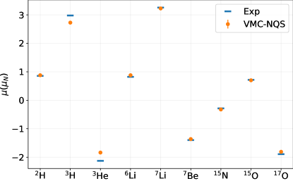
Figure 3: Magnetic moments of selected $A\leq 20$ nuclei obtained from VMC-NQS calculations compared with experimental data.

As shown in Fig. 3, theoretical calculations reproduce experimental data very well, implying that the input LO $\not{\pi}$EFT Hamiltonian encapsulates the essential elements of nuclear structure. This agreement also confirms the correctness of the algorithm discussed for selecting the polarization of the nucleus. Finally, it indicates that NSQ can learn the shell structure of the nucleus, which is genuinely self-emerging as it was not encoded in the variational ansatz. The minor discrepancies observed in ³H, and ³He, are consistent with GFMC, AFDMC and HH results Pastore et al. (2013); Gnech and Schiavilla (2022); Martin et al. (2023) and may well be resolved when two-body currents are included in the calculation.

Conclusions –

With the overarching aim of elucidating the essential aspects of nuclear binding, we accurately computed ground-state properties of atomic nuclei containing up to $A=20$ nucleons using as input the LO $\not{\pi}$EFT Hamiltonian “o” of Ref. Schiavilla et al. (2021). To achieve precise solutions to the many-body Schrödinger equation, we employed a VMC method based on the versatile hidden-nucleon NQS framework, introduced in Ref. Lovato et al. (2022b). Taking inspiration from condensed-matter studies Pescia et al. (2023); Kim et al. (2023), we significantly enhanced the convergence and expressive power of the original hidden-nucleon ansatz by employing equivariant backflow transformations based on MPNN to preprocess the single-nucleon coordinates and incorporate correlation effects.

In line with the findings of Ref. Lu et al. (2019), which employed a spin-isospin independent, non-local, SU(4)-symmetric Hamiltonian, our computed binding energies typically exhibit deviations of only a few percent from experimental values. This level of precision is particularly remarkable considering the simplicity of the input Hamiltonian, especially when compared to the more sophisticated N²LO chiral-EFT interactions that struggle to replicate ground-state energies with comparable accuracy Martin et al. (2023). Furthermore, the $\not{\pi}$EFT model “o” considered in this work — albeit with a slightly different value for the three-body force regulator — yields a neutron-matter equation of state that closely resembles the one obtained from the highly-realistic Argonne $v_{18}$ plus Urbana IX potentials Fore et al. (2023). This contrasts with the $\Delta$-full chiral-EFT Hamiltonian “NV2+Ia,” which provides an accurate energy spectrum for $A\leq 12$ nuclei Piarulli et al. (2018), yet falters in accurately modeling infinite neutron matter Lovato et al. (2022a). We ascribe the surprising accuracy of our “essential” Hamiltonian to a combination of two factors: i) the two-body potential reproduces peripheral, low-energy nucleon-nucleon scattering, and ii) the three-body force prevents nucleons from packing too closely, making low-momentum observables, such as binding energies and radii, insensitive to short-range details of the nuclear force.

Unlike quantum many-body methods based on single-particle basis expansion Barrett et al. (2013); Caprio et al. (2022), and akin to conventional QMC methods, NQS have no difficulties in capturing the slowly-decaying tails of nuclear wave functions, which play a crucial role in reproducing charge radii. Our theoretical calculations align reasonably well with experiments, although some discrepancies are present. Hence, similar to high-precision chiral-EFT forces Somà et al. (2020), charge radii offer additional insights into nuclear dynamics not provided by binding energies alone Garcia Ruiz et al. (2016); Koszorús et al. (2021).

Lastly, we introduced an innovative computational protocol to assess magnetic moments, amenable to NQS. It involves adding to the nuclear Hamiltonian an external magnetic field, which projects the NQS onto a specified value of the orbital angular momentum along the $z$ axis. Our computed magnetic dipole moments are in good agreement with experimental data; the discrepancies observed in ³H and ³He are likely to be resolved with the inclusion of two-body currents Pastore et al. (2013); Martin et al. (2023); Gnech and Schiavilla (2022). Beyond serving as an additional test for the underlying Hamiltonian, this concordance reveals how nucleons self-organize within shells, a structural aspect of the nucleus that is not explicitly embedded within the NQS ansatz but reveal its flexibility.

*

Appendix A Appendix: Wigner-Eckart

In this Section, we outline the procedure used to compute the magnetic moments of nuclei with $J<L+S$, such as ¹⁵O and ¹⁵N. The starting point are the NQS with with good $L_{z}$, which are linear combinations of $J$, $J_{z}$ eigenstates

$$|L,L_{z};S,S_{z}\rangle=\sum_{J,J_{z}}\langle L,L_{z};S,S_{z}|J,J_{z}\rangle|J,J_{z}\rangle\,,$$ (4)

where $\langle L,L_{z};S,S_{z}|J,J_{z}\rangle$ are the Clebsch-Gordan coefficient Workman and Others (2022). We define the magnetic moments of these states as

$$\mu_{L_{z}}=\langle L,L_{z};S,S_{z}|\hat{\mu_{z}}|L;L_{z};S,S_{z}\rangle\,.\,.$$ (5)

Exploiting the Wigner-Eckart theorem, these matrix elements can be expressed in terms of the reduced matrix elements $\langle J||\hat{\mu_{z}}||J^{\prime}\rangle$ as

$$\mu_{L_{z}} =\sum_{J,J_{z},J^{\prime},J_{z}^{\prime}}\langle L,L_{z};S,S_{z}|J,J_{z}\rangle\langle L,L_{z};S,S_{z}|J^{\prime},J^{\prime}_{z}\rangle$$

$$\times\frac{\langle J^{\prime},J_{z}^{\prime};1,0|JJ_{z}\rangle}{\sqrt{2J+1}}\langle J||\hat{\mu_{z}}||J^{\prime}\rangle\,,\,,$$ (6)

with $\langle J||\hat{\mu_{z}}||J^{\prime}\rangle=\langle J^{\prime}||\hat{\mu_{z}}||J\rangle$. The latter can be found by solving a linear systems of equations, provided enough $\mu_{L_{z}}$ are independently evaluated. From the reduced matrix elements, it is immediate to obtain the physical ones by exploiting again the Wigner-Eckart theorem

$$\langle J,J_{z}|\hat{\mu}_{z}|J,J_{z}\rangle=\frac{\langle J,J_{z};1,0|J,J_{z}\rangle}{\sqrt{2J+1}}\langle J||\hat{\mu}_{z}||J\rangle\,.$$ (7)

The ¹⁵O and ¹⁵N nuclei are both $(J=1/2^{+})$ and the NQS converges to $L=1$ and $S=1/2$. For each nucleus we calculated the matrix elements in Eq. (5) with $L_{z}=0,+1$, and $-1$ ($S_{z}$ is conveniently fixed in the Metropolis Hastings Sampling to the value $S_{z}=1/2$). Solving the linear system generated by Eq. (6), we obtain the magnetic moment matrix element for the physical state $J=1/2$ and $J_{z}=1/2$ as function of $\mu_{L_{z}}$, which has the compact expression

$$\mu_{J=1/2}=\langle 1/2,1/2|\hat{\mu}_{z}|1/2,1/2\rangle=\mu_{0}-\mu_{-1}-\frac{1}{3}\mu_{+1}\,.$$ (8)

References

- Hergert (2020) H. Hergert, “A Guided Tour of Nuclear Many-Body Theory,” Front. in Phys. 8, 379 (2020), arXiv:2008.05061 [nucl-th] .
- Wiringa et al. (1995) Robert B. Wiringa, V. G. J. Stoks, and R. Schiavilla, “An Accurate nucleon-nucleon potential with charge independence breaking,” Phys. Rev. C 51, 38–51 (1995), arXiv:nucl-th/9408016 .
- Machleidt (2001) R. Machleidt, “The High precision, charge dependent Bonn nucleon-nucleon potential (CD-Bonn),” Phys. Rev. C 63, 024001 (2001), arXiv:nucl-th/0006014 .
- Entem and Machleidt (2003) D. R. Entem and R. Machleidt, “Accurate charge dependent nucleon nucleon potential at fourth order of chiral perturbation theory,” Phys. Rev. C 68, 041001 (2003), arXiv:nucl-th/0304018 .
- Epelbaum et al. (2005) E. Epelbaum, W. Glockle, and Ulf-G. Meissner, “The Two-nucleon system at next-to-next-to-next-to-leading order,” Nucl. Phys. A 747, 362–424 (2005), arXiv:nucl-th/0405048 .
- Gezerlis et al. (2013) A. Gezerlis, I. Tews, E. Epelbaum, S. Gandolfi, K. Hebeler, A. Nogga, and A. Schwenk, “Quantum Monte Carlo Calculations with Chiral Effective Field Theory Interactions,” Phys. Rev. Lett. 111, 032501 (2013), arXiv:1303.6243 [nucl-th] .
- Lynn et al. (2016) J. E. Lynn, I. Tews, J. Carlson, S. Gandolfi, A. Gezerlis, K. E. Schmidt, and A. Schwenk, “Chiral Three-Nucleon Interactions in Light Nuclei, Neutron- Scattering, and Neutron Matter,” Phys. Rev. Lett. 116, 062501 (2016), arXiv:1509.03470 [nucl-th] .
- Epelbaum et al. (2015) E. Epelbaum, H. Krebs, and U. G. Meißner, “Precision nucleon-nucleon potential at fifth order in the chiral expansion,” Phys. Rev. Lett. 115, 122301 (2015), arXiv:1412.4623 [nucl-th] .
- Piarulli et al. (2015) M. Piarulli, L. Girlanda, R. Schiavilla, R. Navarro Pérez, J. E. Amaro, and E. Ruiz Arriola, “Minimally nonlocal nucleon-nucleon potentials with chiral two-pion exchange including resonances,” Phys. Rev. C 91, 024003 (2015), arXiv:1412.6446 [nucl-th] .
- Entem et al. (2017) D. R. Entem, R. Machleidt, and Y. Nosyk, “High-quality two-nucleon potentials up to fifth order of the chiral expansion,” Phys. Rev. C 96, 024004 (2017), arXiv:1703.05454 [nucl-th] .
- Piarulli et al. (2018) M. Piarulli et al., “Light-nuclei spectra from chiral dynamics,” Phys. Rev. Lett. 120, 052503 (2018), arXiv:1707.02883 [nucl-th] .
- Barrett et al. (2013) Bruce R. Barrett, Petr Navratil, and James P. Vary, “Ab initio no core shell model,” Prog. Part. Nucl. Phys. 69, 131–181 (2013).
- Hagen et al. (2014) G. Hagen, T. Papenbrock, M. Hjorth-Jensen, and D. J. Dean, “Coupled-cluster computations of atomic nuclei,” Rept. Prog. Phys. 77, 096302 (2014), arXiv:1312.7872 [nucl-th] .
- Hergert et al. (2016) H. Hergert, S. K. Bogner, T. D. Morris, A. Schwenk, and K. Tsukiyama, “The In-Medium Similarity Renormalization Group: A Novel Ab Initio Method for Nuclei,” Phys. Rept. 621, 165–222 (2016), arXiv:1512.06956 [nucl-th] .
- Carbone et al. (2013) Arianna Carbone, Andrea Cipollone, Carlo Barbieri, Arnau Rios, and Artur Polls, “Self-consistent Green’s functions formalism with three-body interactions,” Phys. Rev. C 88, 054326 (2013), arXiv:1310.3688 [nucl-th] .
- Epelbaum et al. (2011) Evgeny Epelbaum, Hermann Krebs, Dean Lee, and Ulf-G. Meissner, “Ab initio calculation of the Hoyle state,” Phys. Rev. Lett. 106, 192501 (2011), arXiv:1101.2547 [nucl-th] .
- Carlson et al. (2015) J. Carlson, S. Gandolfi, F. Pederiva, Steven C. Pieper, R. Schiavilla, K. E. Schmidt, and R. B. Wiringa, “Quantum Monte Carlo methods for nuclear physics,” Rev. Mod. Phys. 87, 1067 (2015), arXiv:1412.3081 [nucl-th] .
- Morris et al. (2018) T. D. Morris, J. Simonis, S. R. Stroberg, C. Stumpf, G. Hagen, J. D. Holt, G. R. Jansen, T. Papenbrock, R. Roth, and A. Schwenk, “Structure of the lightest tin isotopes,” Phys. Rev. Lett. 120, 152503 (2018), arXiv:1709.02786 [nucl-th] .
- Hu et al. (2022) Baishan Hu et al., “Ab initio predictions link the neutron skin of 208Pb to nuclear forces,” Nature Phys. 18, 1196–1200 (2022), arXiv:2112.01125 [nucl-th] .
- Binder et al. (2014) Sven Binder, Joachim Langhammer, Angelo Calci, and Robert Roth, “Ab Initio Path to Heavy Nuclei,” Phys. Lett. B 736, 119–123 (2014), arXiv:1312.5685 [nucl-th] .
- Lonardoni et al. (2017) D. Lonardoni, A. Lovato, Steven C. Pieper, and R. B. Wiringa, “Variational calculation of the ground state of closed-shell nuclei up to ,” Phys. Rev. C 96, 024326 (2017), arXiv:1705.04337 [nucl-th] .
- Sammarruca and Millerson (2021) Francesca Sammarruca and Randy Millerson, “Overview of symmetric nuclear matter properties from chiral interactions up to fourth order of the chiral expansion,” Phys. Rev. C 104, 064312 (2021), arXiv:2109.01985 [nucl-th] .
- Nosyk et al. (2021) Y. Nosyk, D. R. Entem, and R. Machleidt, “Nucleon-nucleon potentials from -full chiral effective-field-theory and implications,” Phys. Rev. C 104, 054001 (2021), arXiv:2107.06452 [nucl-th] .
- Lovato et al. (2022a) A. Lovato, I. Bombaci, D. Logoteta, M. Piarulli, and R. B. Wiringa, “Benchmark calculations of infinite neutron matter with realistic two- and three-nucleon potentials,” Phys. Rev. C 105, 055808 (2022a), arXiv:2202.10293 [nucl-th] .
- Lu et al. (2019) Bing-Nan Lu, Ning Li, Serdar Elhatisari, Dean Lee, Evgeny Epelbaum, and Ulf-G. Meißner, “Essential elements for nuclear binding,” Phys. Lett. B 797, 134863 (2019), arXiv:1812.10928 [nucl-th] .
- Kievsky et al. (2018) A. Kievsky, M. Viviani, D. Logoteta, I. Bombaci, and L. Girlanda, “Correlations imposed by the unitary limit between few-nucleon systems, nuclear matter and neutron stars,” Phys. Rev. Lett. 121, 072701 (2018), arXiv:1806.02636 [nucl-th] .
- Lee et al. (2021) Dean Lee et al., “Hidden Spin-Isospin Exchange Symmetry,” Phys. Rev. Lett. 127, 062501 (2021), arXiv:2010.09420 [nucl-th] .
- Kievsky et al. (2021) A. Kievsky, L. Girlanda, M. Gattobigio, and M. Viviani, “Efimov Physics and Connections to Nuclear Physics,” Ann. Rev. Nucl. Part. Sci. 71, 465–490 (2021), arXiv:2102.13504 [nucl-th] .
- Bedaque and van Kolck (2002) Paulo F. Bedaque and Ubirajara van Kolck, “Effective field theory for few nucleon systems,” Ann. Rev. Nucl. Part. Sci. 52, 339–396 (2002), arXiv:nucl-th/0203055 .
- Schiavilla et al. (2021) R. Schiavilla, L. Girlanda, A. Gnech, A. Kievsky, A. Lovato, L. E. Marcucci, M. Piarulli, and M. Viviani, “Two- and three-nucleon contact interactions and ground-state energies of light- and medium-mass nuclei,” Phys. Rev. C 103, 054003 (2021), arXiv:2102.02327 [nucl-th] .
- Fore et al. (2023) Bryce Fore, Jane M. Kim, Giuseppe Carleo, Morten Hjorth-Jensen, Alessandro Lovato, and Maria Piarulli, “Dilute neutron star matter from neural-network quantum states,” Phys. Rev. Res. 5, 033062 (2023), arXiv:2212.04436 [nucl-th] .
- Emery (2006) Guy Emery, “Hyperfine structure,” in Springer Handbook of Atomic, Molecular, and Optical Physics, edited by Gordon Drake (Springer New York, New York, NY, 2006) pp. 253–260.
- Bohr and Mottelson (1998) Aage Bohr and Ben R Mottelson, Nuclear Structure (World Scientific Publishing Company, 1998) https://www.worldscientific.com/doi/pdf/10.1142/3530 .
- Marcucci et al. (2008) L. E. Marcucci, Muslema Pervin, Steven C. Pieper, R. Schiavilla, and R. B. Wiringa, “Quantum Monte Carlo calculations of magnetic moments and M1 transitions in A=7 nuclei including meson-exchange currents,” Phys. Rev. C 78, 065501 (2008), arXiv:0810.0547 [nucl-th] .
- Pastore et al. (2013) S. Pastore, Steven C. Pieper, R. Schiavilla, and R. B. Wiringa, “Quantum Monte Carlo calculations of electromagnetic moments and transitions in A 9 nuclei with meson-exchange currents derived from chiral effective field theory,” Phys. Rev. C 87, 035503 (2013), arXiv:1212.3375 [nucl-th] .
- Martin et al. (2023) J. D. Martin, S. J. Novario, D. Lonardoni, J. Carlson, S. Gandolfi, and I. Tews, “Auxiliary field diffusion Monte Carlo calculations of magnetic moments of light nuclei with chiral EFT interactions,” (2023), arXiv:2301.08349 [nucl-th] .
- Gandolfi et al. (2014) S. Gandolfi, A. Lovato, J. Carlson, and Kevin E. Schmidt, “From the lightest nuclei to the equation of state of asymmetric nuclear matter with realistic nuclear interactions,” Phys. Rev. C 90, 061306 (2014), arXiv:1406.3388 [nucl-th] .
- Keeble and Rios (2020) J. W. T. Keeble and A. Rios, “Machine learning the deuteron,” Phys. Lett. B 809, 135743 (2020), arXiv:1911.13092 [nucl-th] .
- Adams et al. (2021) Corey Adams, Giuseppe Carleo, Alessandro Lovato, and Noemi Rocco, “Variational Monte Carlo Calculations of A4 Nuclei with an Artificial Neural-Network Correlator Ansatz,” Phys. Rev. Lett. 127, 022502 (2021), arXiv:2007.14282 [nucl-th] .
- Gnech et al. (2022) Alex Gnech, Corey Adams, Nicholas Brawand, Giuseppe Carleo, Alessandro Lovato, and Noemi Rocco, “Nuclei with up to nucleons with artificial neural network wave functions,” Few Body Syst. 63, 7 (2022), arXiv:2108.06836 [nucl-th] .
- Yang and Zhao (2022) Y. L. Yang and P. W. Zhao, “A consistent description of the relativistic effects and three-body interactions in atomic nuclei,” Phys. Lett. B 835, 137587 (2022), arXiv:2206.13208 [nucl-th] .
- Lovato et al. (2022b) Alessandro Lovato, Corey Adams, Giuseppe Carleo, and Noemi Rocco, “Hidden-nucleons neural-network quantum states for the nuclear many-body problem,” Phys. Rev. Res. 4, 043178 (2022b), arXiv:2206.10021 [nucl-th] .
- Luo and Clark (2019) Di Luo and Bryan K. Clark, “Backflow transformations via neural networks for quantum many-body wave functions,” Phys. Rev. Lett. 122, 226401 (2019).
- Pescia et al. (2023) Gabriel Pescia, Jannes Nys, Jane Kim, Alessandro Lovato, and Giuseppe Carleo, “Message-Passing Neural Quantum States for the Homogeneous Electron Gas,” (2023), arXiv:2305.07240 [quant-ph] .
- Kim et al. (2023) Jane Kim, Gabriel Pescia, Bryce Fore, Jannes Nys, Giuseppe Carleo, Stefano Gandolfi, Morten Hjorth-Jensen, and Alessandro Lovato, “Neural-network quantum states for ultra-cold Fermi gases,” (2023), arXiv:2305.08831 [cond-mat.quant-gas] .
- Moreno et al. (2022) Javier Robledo Moreno, Giuseppe Carleo, Antoine Georges, and James Stokes, “Fermionic wave functions from neural-network constrained hidden states,” Proceedings of the National Academy of Sciences of the United States of America 119, e2122059119 (2022).
- Zaheer et al. (2017) Manzil Zaheer, Satwik Kottur, Siamak Ravanbakhsh, Barnabas Poczos, Ruslan Salakhutdinov, and Alexander Smola, “Deep Sets,” arXiv e-prints , arXiv:1703.06114 (2017), arXiv:1703.06114 [cs.LG] .
- Wagstaff et al. (2019) Edward Wagstaff, Fabian B. Fuchs, Martin Engelcke, Ingmar Posner, and Michael Osborne, “On the Limitations of Representing Functions on Sets,” arXiv e-prints , arXiv:1901.09006 (2019), arXiv:1901.09006 [cs.LG] .
- Lonardoni et al. (2018) D. Lonardoni, S. Gandolfi, J. E. Lynn, C. Petrie, J. Carlson, K. E. Schmidt, and A. Schwenk, “Auxiliary field diffusion Monte Carlo calculations of light and medium-mass nuclei with local chiral interactions,” Phys. Rev. C 97, 044318 (2018), arXiv:1802.08932 [nucl-th] .
- Gandolfi et al. (2020) Stefano Gandolfi, Diego Lonardoni, Alessandro Lovato, and Maria Piarulli, “Atomic nuclei from quantum Monte Carlo calculations with chiral EFT interactions,” Front. in Phys. 8, 117 (2020), arXiv:2001.01374 [nucl-th] .
- Sorella (2005) Sandro Sorella, “Wave function optimization in the variational Monte Carlo method,” Phys. Rev. B 71, 241103 (2005).
- Maris et al. (2021) P. Maris et al., “Light nuclei with semilocal momentum-space regularized chiral interactions up to third order,” Phys. Rev. C 103, 054001 (2021), arXiv:2012.12396 [nucl-th] .
- Ong et al. (2010) A. Ong, J. C. Berengut, and V. V. Flambaum, “The Effect of spin-orbit nuclear charge density corrections due to the anomalous magnetic moment on halonuclei,” Phys. Rev. C 82, 014320 (2010), arXiv:1006.5508 [nucl-th] .
- Lovato et al. (2013) A. Lovato, S. Gandolfi, Ralph Butler, J. Carlson, Ewing Lusk, Steven C. Pieper, and R. Schiavilla, “Charge Form Factor and Sum Rules of Electromagnetic Response Functions in ,” Phys. Rev. Lett. 111, 092501 (2013), arXiv:1305.6959 [nucl-th] .
- Caprio et al. (2022) Mark A. Caprio, Patrick J. Fasano, and Pieter Maris, “Robust ab initio prediction of nuclear electric quadrupole observables by scaling to the charge radius,” Phys. Rev. C 105, L061302 (2022), arXiv:2206.09307 [nucl-th] .
- Gnech and Schiavilla (2022) A. Gnech and R. Schiavilla, “Magnetic structure of few-nucleon systems at high momentum transfers in a chiral effective field theory approach,” Phys. Rev. C 106, 044001 (2022).
- Somà et al. (2020) V. Somà, P. Navrátil, F. Raimondi, C. Barbieri, and T. Duguet, “Novel chiral Hamiltonian and observables in light and medium-mass nuclei,” Phys. Rev. C 101, 014318 (2020), arXiv:1907.09790 [nucl-th] .
- Garcia Ruiz et al. (2016) R. F. Garcia Ruiz et al., “Unexpectedly large charge radii of neutron-rich calcium isotopes,” Nature Phys. 12, 594 (2016), arXiv:1602.07906 [nucl-ex] .
- Koszorús et al. (2021) Á. Koszorús et al., “Charge radii of exotic potassium isotopes challenge nuclear theory and the magic character of ,” Nature Phys. 17, 439–443 (2021), [Erratum: Nature Phys. 17, 539 (2021)], arXiv:2012.01864 [nucl-ex] .
- Workman and Others (2022) R. L. Workman and Others (Particle Data Group), “Review of Particle Physics,” PTEP 2022, 083C01 (2022).
*