Neutrino anisotropy as a probe of extreme astrophysical accelerators

Abstract

We consider how the cutoff of the ultrahigh energy neutrino spectrum introduces an effective neutrino horizon, allowing for future neutrino detectors to measure an anisotropy in neutrino arrival directions driven by the local large-scale structure. We show that measurement of the level of this anisotropy along with features of the neutrino spectrum will allow for a measurement of the evolution of ultrahigh energy neutrino sources, which are expected to also be the sources of ultrahigh energy cosmic rays.

Introduction—Discovery of a diffuse flux of neutrinos has opened a new window on the universe. The diffuse neutrino spectrum observed from $\sim 10$ TeV to $\sim 10$ PeV [1, 2] could in principle extend up beyond EeV energies, since neutrinos are produced exclusively through cosmic ray interactions and those are observed up to $\sim$100 EeV. Below roughly $10$ PeV, cosmic rays produced by a variety of (Galactic and extragalactic) accelerators can contribute to the diffuse neutrino spectrum. Up to now, no significant neutrino anisotropy or correlation with sources has been found [3, 4, 5, 6, 7, 8, 9, 10, 11, 12], though a correlation with the Galactic plane emerges at low energies [13]. Above $10$ PeV, only cosmic rays produced by the most extreme accelerators, ultrahigh energy cosmic rays (UHECRs, $E_{CR}\gtrsim 100$ PeV), have sufficient energy to contribute to the diffuse UHE neutrino spectrum.

The sources of UHECRs remain an open question in astroparticle physics [14]. UHECRs themselves probe only the most local sources (within $100$ Mpc at $100$ EeV) due to horizons imprinted by the Greisen-Zatsepin-Kuzmin (GZK) effect [15, 16] and time delays from extragalactic magnetic fields [17]. Moreover, UHECRs which do reach Earth undergo large deflections in the Galactic magnetic field [18], making source identification extremely challenging. UHE neutrinos, however, represent an unprecedented window into UHECR sources since they both point back to their sources and probe cosmological distances.

A cutoff has been observed in the UHECR spectrum around $10^{19.7}$ eV [19]. This implies that the UHE neutrino spectrum should also have a cutoff related to the maximum UHECR energy at the accelerator. Since neutrinos suffer adiabatic losses due to the expansion of the universe and “redshift” to lower energies, neutrinos observed near the cutoff energy necessarily come from local sources. In this Letter, we show that a significant anisotropy must exist around the cutoff energy of the neutrino spectrum, and propose that it provides a powerful new tool for investigating the origin of diffuse UHE neutrinos.

Model—Recent studies [20, 21] have shown that the UHECR dipole is likely to originate from the large-scale structure (LSS) of the local universe, whose imprint on the sky is then transformed by Galactic magnetic field lensing effects. This result depends on two key insights: first, that the distribution of UHECR accelerators should follow the matter distribution; and second, that the extragalactic background light (EBL), cosmic microwave background (CMB), and intervening magnetic fields introduce a horizon to the UHECR observable universe. This horizon ensures that the local LSS is the most prominent structure in the UHECR sky, rather than the homogeneous, isotropic universe at higher redshifts.

The neutrino sky will also have a horizon, albeit a much larger one generally, near the cutoff of the neutrino spectrum $E_{\mathrm{max}}$. An observer integrating the neutrino spectrum above a threshold energy $E_{\mathrm{th}}$ will introduce a neutrino horizon, since all neutrinos beyond a redshift $z_{\mathrm{max}}=E_{\mathrm{max}}/E_{\mathrm{th}}-1$ will arrive at Earth with energies below this threshold. For example, if $E_{\mathrm{th}}=0.9E_{\mathrm{max}}$, then neutrinos will only probe sources within $z<z_{\mathrm{max}}\sim 0.11$ (roughly $460$ Mpc comoving distance). If $E_{\mathrm{max}}$ is a soft cutoff energy (e.g. the energy scale in an exponential cutoff), then this horizon will also be gradual. We quantify the redshift of this soft horizon, $z_{99}$, as the redshift beyond which $\geq 99\%$ of a source’s above threshold comoving flux has redshifted below threshold. This allows the observer to “tune” the energy threshold to probe an arbitrarily small volume of the universe, provided a sufficiently large detector and the existence of UHE neutrino sources within this local volume.

Astrophysical neutrinos are produced when UHECRs interact with ambient gas and photons at the acceleration sites or in their source environments [22]. This implies that if UHECR sources follow the matter distribution of the universe, then so will astrophysical neutrino sources. If neutrino sources are negatively evolving (decreasing luminosity-density with redshift) observers will measure the neutrino sky to by highly anisotropic, following the local distribution of matter as in the case of UHECRs. By constrast, in the case where the evolution of neutrino sources is positive (increasing luminosity-density with redshift), this anisotropy will be much weaker. However, the local LSS can still leave a measurable imprint on the neutrino sky which observers can enhance by tuning their energy threshold. This guarantees that the UHE neutrino sky is anisotropic at energies sufficiently close to the spectrum cutoff.

To quantify the level of anisotropy we make a few simplifying assumptions. First, we assume all sources emit a common neutrino spectrum, $Q_{\nu}(E)$, and that this astrophysical spectrum is the dominant contribution to the observed UHE neutrino spectrum. Evidence for the former assumption has been found for UHECR source spectra [23]. Second, we assume that the neutrino source density at low redshifts follows the spatial distribution of the local LSS matter density, whereas at high redshifts it is nearly isotropic. Importantly the total flux from a given redshift depends on the source luminosity-density with redshift, $\mathcal{H}(z)$, rather than the source density alone.

To realistically model the distribution of the local LSS we use the quasi-linear density field from CosmicFlows-2, which is based on an ensemble of $20$ constrained realizations of the local (within $360$ Mpc) universe [24]. A view of this median density field is shown at https://skfb.ly/6AFxT. The density field beyond the box boundaries is obtained in the linear regime using a series of constrained linear realizations (based on the linear WF/CRs algorithm [25, 26]) within a $1830$ Mpc depth. The use of the linear realizations is justified as the contributions to the anisotropy from beyond the box of $360$ Mpc are dominated by large (linear) scales (see [24] for more details). Beyond $1830$ Mpc we assume the density field fluctuations are small enough to be well-approximated as perfectly isotropic.

The total neutrino flux $J_{\nu}$ above an energy threshold $E_{\mathrm{th}}$ is given by

$$J_{\nu}(E>E_{th})=\frac{c}{4\pi}\int_{0}^{\infty}\frac{dz}{H(z)}\int_{E_{th}}^{\infty}\mathcal{H}(z)Q_{\nu}(z,(1+z)E)dE~{}.$$ (1)

In order to calculate the total neutrino anisotropy one needs to determine how this total flux is distributed on the sky. Adopting a healpix pixelization [27], we obtain the neutrino intensity skymap by calculating the total neutrino flux in each pixel $i$, $J_{\nu,i}$.

The fraction of flux, $f_{j}$, originating from a spherical shell, $j$, spanning from redshift $z_{j}$ to $z_{j}+\Delta z_{j}$ is given by

$$f_{j}=\frac{c}{4\pi J_{\nu}}\int_{z_{j}}^{z_{j}+\Delta z_{j}}\frac{dz}{H(z)}\int_{E_{th}}^{\infty}\mathcal{H}(z)Q_{\nu}(z,(1+z)E)dE~{}.$$ (2)

Within this spherical shell, the neutrino flux will be distributed according to the matter distribution. If the total mass within shell $j$ is $M_{j}$ and the total mass within the voxel subtended by pixel $i$ within shell $j$ is $M_{ij}$, then the voxel will produce $M_{ij}/M_{j}$ of the total flux of the shell. Within a comoving distance of $1830$ Mpc we calculate this ratio using the CosmicFlows-2 database. Beyond $1830$ Mpc, we assume the mass of the shell is isotropically distributed so that $M_{ij}=M_{j}\Omega_{i}/4\pi$, where $\Omega_{i}$ is the solid angle subtended by pixel $i$.

The flux within pixel $i$ is then given by summing over the contributions of each shell

$$J_{\nu,i}=J_{\nu}\displaystyle\sum_{j}f_{j}\frac{M_{ij}}{M_{j}}~{}.$$ (3)

In order to calculate (3), one needs the neutrino source spectrum $Q_{\nu}(E)$ and the source evolution $\mathcal{H}(z)$. In practice, since neutrinos are only affected by redshift losses, the parameters of their spectrum at Earth can be directly related to the parameters of their source spectrum. In particular, the spectral index of the source spectrum is the same as that observed on Earth at energies sufficiently below the observed cutoff energy. The observed cutoff energy can be up to a factor of $5$ lower than the cutoff energy of the source, depending on how positive the source evolution is and how hard the source spectrum is. However, for a given observed spectral index and source evolution one can straight-forwardly relate the observed cutoff energy to that of the source spectrum. For the purposes of illustration, we adopt a single power-law spectrum with an exponential cutoff

$$Q_{\nu}(E)\propto E^{-\gamma}e^{-E/E_{\mathrm{max}}}~{}.$$ (4)

Importantly, the absolute scale of $E_{\mathrm{max}}$ does not matter for the purposes of calculating the neutrino anisotropy, only the ratio $E_{\mathrm{th}}/E_{\mathrm{max}}$.

For simplicity, we use a two-parameter model of the source evolution

$$\mathcal{H}_{m,z_{0}}(z) =\mathcal{H}_{0}\begin{cases}(1+z)^{m}&z\leq z_{0}\\ (1+z_{0})^{m}e^{-(z-z_{0})}&z>z_{0}\end{cases}~{}.$$ (5)

This model is an adequate approximation to many source evolutions obtained from astrophysical observations and allows us to straight-forwardly explore the range of plausible source evolutions.

Finally, as can be seen in Fig. 1, the predicted anisotropy for the neutrino sky has a very particular structure due to the imprint of the local LSS. The neutrino skymap is a sum of this anisotropy and an isotropic contribution from higher redshift sources, which depends on the $E_{\mathrm{th}}/E_{\mathrm{max}}$ ratio, the source spectrum, and the source evolution. Therefore, rather than attempting to measure this anisotropy in terms of its multipole moments, we instead develop a template to characterize the level of anisotropy for a given neutrino skymap prediction. For this template we use the predicted skymap for a case where we expect the anisotropy from the local LSS to be dominant on the sky: a very negative source evolution, $m=-5,z_{0}=2$, with an energy threshold at the cutoff energy $E_{\mathrm{th}}=E_{\mathrm{max}}$. This is not meant to be a realistic observational expectation for a skymap, merely a theoretical prediction which can be used to measure the anisotropy level. One still needs to specify the power law index of the source spectrum in order to generate this template. For this purpose we adopt $\gamma=-2.53$ based on the IceCube Cascades data set [28]. This template could be updated once the true spectral index above $10$ PeV is measured, but we show the sensitivity to a varying spectral index in the next section. The resulting skymap template is shown in Fig. 1 (top).

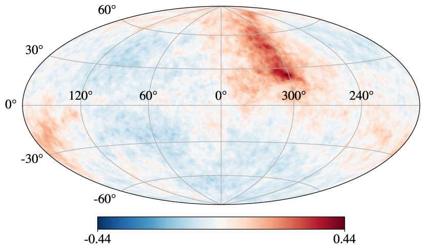
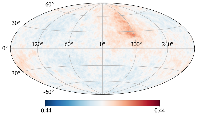
Figure 1: Predicted neutrino skymaps with threshold energies at the maximum neutrino energy for two different source evolution indices: $m=-5$ (top) and $m=0$ (bottom). The color scale indicates the predicted neutrino flux relative to the all-sky average. We assume $z_{0}=2$ and a spectral index of $\gamma=-2.53$. The top skymap serves as the template map for our maximum likelihood analysis.

In order to measure the level of anisotropy of a skymap, $\alpha$, for a given source evolution compared to our template we perform a maximum likelihood analysis. We consider two nested hypotheses: an isotropic skymap as our null hypothesis and a superposition of an isotropic skymap and a local LSS anisotropy template as our alternative hypothesis. Under this framework the average number of neutrino events predicted in pixel $i$, $\mu_{i}$, is given by

$$\mu_{i}=\left[\alpha\frac{J_{\nu,i}}{J_{\nu}}+(1-\alpha)\frac{\Omega_{i}}{4\pi}\right]N_{\mathrm{evts}}~{},$$ (6)

where $\alpha$ is the relative weight of the anisotropy template ($\alpha=0$ corresponding to the null hypothesis) and $N_{\mathrm{evts}}$ is the total number of neutrino events in the skymap. Given a set of observed neutrinos $n_{i}$, the likelihood is then given by the product of Poisson probabilities

$$\mathcal{L}(\alpha|n_{i})=\prod_{i}\mathrm{Poiss}(n_{i}|\mu_{i})~{}.$$ (7)

With this definition we obtain an estimate of $\alpha$ by maximizing the log-likelihood ratio $\ln\left(\mathcal{L}(\alpha|n_{i})/\mathcal{L}(0|n_{i})\right)$. In the limit of large statistics, we use this maximum likelihood estimate (MLE) of $\alpha$ to measure the level of neutrino anisotropy for a predicted skymap.

Results—Figure 1 illustrates the predicted neutrino anisotropy for two source evolutions: $m=-5$ and $m=0$. In both cases the energy threshold is at the cutoff energy so as to amplify the anisotropy from the local LSS. Specifically for the spectral index considered, this energy threshold results in a soft horizon of $z_{99}\simeq 1.65$. These plots clearly demonstrate the isotropizing effect of having more sources at high redshifts (as is the case for more positive source evolutions).

The dependence of the predicted level of anisotropy on source evolution is shown in Fig. 2. As can be seen, there is a strong dependence of the level of anisotropy on the source evolution. Since the unknown parameters assumed in this plot can be measured directly (the neutrino spectral index and cutoff energy) or are set by the observer (the threshold energy) it is possible for observers to accurately measure this quantity. Observers can use this anisotropy measurement to directly measure the evolution of UHE neutrino sources – and therefore of UHECR sources. Moreover, it is possible to place a lower-bound on the value of $m$ even in the case that an observer can only place an upper-bound on the value of $\alpha$. Such a strong constraint on $m$ would result in a significant improvement in UHECR source modeling and a major step towards determining their sources.

From Fig. 2 it is also clear that even for small threshold energies, where essentially no horizon exists, there is a minimum level of anisotropy due to the imprint of the local LSS. For more negative source evolutions this minimum level of anisotropy can be significant. This fact means that even if observatories are not yet sensitive enough to determine the cutoff energy, observers may still be able to measure a significant anisotropy in the neutrino sky. We note that one could conduct such an analysis with $E_{\mathrm{th}}<10$ PeV. However, the resulting anisotropy will be due to a mix of UHE and lower energy neutrino sources.

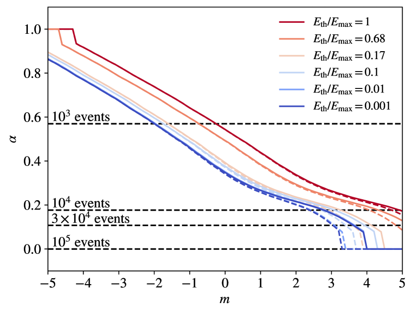
Figure 2: Anisotropy measure $\alpha$ as a function of source evolution power law index $m$ for various threshold energies (colored lines). All lines assume $\gamma=-2.53$ and $z_{0}=2$ (solid) or $z_{0}=4$ (dashed). Dashed black lines indicate the $90\%$ confidence level upper-limit on $\alpha$ given a number of observed events for a truly isotropic distribution. Note that $\alpha$ saturates to $1$ $(0)$ once the level of anisotropy is maximized (minimized).

In principle, observers will have a more sensitive measurement of the anisotropy if they know the true spectral index of the neutrino spectrum when building an anisotropy template. However, Fig. 3 shows the sensitivity of the level of anisotropy to the spectral index when using a template with fixed spectral index. The level of anisotropy decreases for harder spectral indices. This is expected since harder spectral indices place a larger fraction of the source spectrum at high energies, effectively pushing the cutoff to slightly higher energies. This gives this makes the soft horizon more gradual so that a larger fraction of the total flux comes from sources at high redshifts.

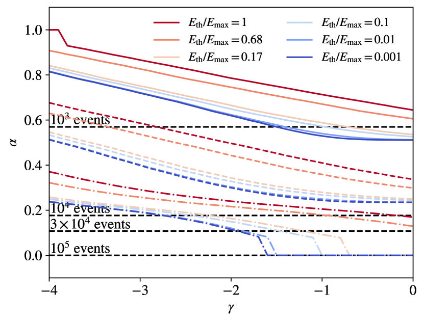
Figure 3: Sensitivity of the anisotropy measure to the source spectral index for various $E_{\mathrm{th}}/E_{\mathrm{max}}$ ratios (colored lines). All MLEs of $\alpha$ were calculated using a template with $\gamma=-2.53$ and $m=-5$. Results are shown for several source evolutions ($z_{0}=2$ fixed): $m=+3$ (solid), $m=0$ (dashed), and $m=-3$ (dash dotted).

Discussion—While the results discussed above represent a significant observational opportunity, they also represent a significant observational challenge. Positive source evolutions will have an inherently small neutrino anisotropy, making the exact source evolution difficult to measure. This situation can be improved slightly by raising the energy threshold to amplify the level of anisotropy, but this necessarily will decrease the number of neutrinos that can be used in such an analysis. A decrease in statistics makes confidently rejecting the null hypothesis challenging. Figure 4 shows the $90\%$ confidence level (CL) upper-limit on $\alpha$ for realizations of an isotropic distribution with a fixed number of events. From this on can see that even for negative source evolutions, where the level of anisotropy may be quite significant, a statistically significant measurement of the neutrino anisotropy will require $\mathcal{O}(10^{3})$ neutrinos.

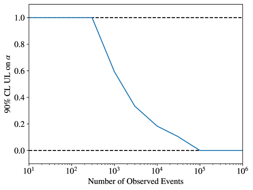
Figure 4: $90\%$ CL upper-limit of the maximum likelihood estimate of $\alpha$ for events sampled from a truly isotropic distribution. More than $300$ events are required to set a meaningful upper-limit ($\alpha<1$), while $10^{5}$ events are sufficient to completely distinguish isotropy from $\alpha\neq 0$ scenarios at $90\%$ CL.

Throughout this Letter we have assumed the observed neutrino flux is dominated by neutrinos of astrophysical origin. The flux of cosmogenic neutrinos depends on the details of the UHECR spectrum escaping the source. However, the majority of the cosmogenic neutrino flux arriving at Earth is produced by UHECRs originating from sources at higher redshifts and will therefore inherit the isotropy of high redshift sources. Thus, a cosmogenic contribution to the observed neutrino flux will mostly serve to reduce the level of anisotropy but a specific model of the UHECR flux escaping sources is required to quantify by how much. It is worth noting, however, that some energy regimes are more likely to be dominated by astrophysical neutrinos than others. In particular, UHECR source modeling [29] shows that neutrinos in the $1-100$ PeV range are likely to be dominantly produced inside sources, while those $\gtrsim 1$ EeV are likely to be equally, or dominantly in some cases, of cosmogenic origin. However, the evolution of $\gtrsim$ EeV neutrino sources can be constrained using other methods [30].

Strong extragalactic magnetic fields around filaments may increase the residence time of UHECRs in their source clusters [31]. This would serve to produce an additional neutrino flux contribution which traces the matter distribution of the universe, thereby further increasing the neutrino anisotropy. However, this effect is strongly model dependent and is beyond the scope of this study.

Finally we note that the bias between the normal matter and dark matter density fields may affect the exact level of neutrino anisotropy. This bias can depend on the properties of the galaxy host to the neutrino source, which may lead some source types to produce neutrino anisotropies which are not well-represented by the simple model described above. We leave investigation of this effect for future work.

Summary—In this Letter we investigated the anisotropy of the UHE neutrino sky due to the LSS and demonstrated how observers can enhance this anisotropy by selecting an energy threshold. We found that the level of anisotropy can be used to constrain the evolution of UHE neutrino sources. Given the expectation that UHE neutrinos are produced by UHECRs, such a measurement would place strong constraints on the evolution of UHECR sources and provide a significant evidence as to their origin.

To measure this anisotropy, we showed that a large UHE neutrino data set is required. This suggests that such a measurement will need to be a coordinated effort among the next generation of UHE neutrino observatories, such as IceCube-Gen2 [32] and GRAND [33]. However, until neutrinos at UHEs are measured, the plausibility of creating such a data set is unclear (though it is within the realm of theoretical possibility [30]). To overcome this one could investigate the level of neutrino anisotropy taking a threshold energy below $10$ PeV. However the result will trace the evolution of lower energy neutrino sources, which may be distinct from that of UHE neutrino & UHECR sources.

Beyond measurement of the source evolution, observation of the LSS neutrino anisotropy would represent a major breakthrough for UHECR studies. In particular, it would provide an independent confirmation of the origin of the UHECR dipole. Moreover, this would provide an additional constraint on models of the Galactic magnetic field which predict significantly different UHECR deflections but otherwise fit observational data equally well [34].