Aspects of Particle Production from Bubble Dynamics
at a First Order Phase Transition

Abstract

First order phase transitions (FOPTs) constitute an active area of contemporary research as a promising cosmological source of observable gravitational waves. The spacetime dynamics of the background scalar field undergoing the phase transition can also directly produce quanta of particles that couple to the scalar, which has not been studied as extensively in the literature. This paper provides the first careful examination of various important aspects of this phenomenon. In particular, the contributions from various stages of FOPTs (bubble nucleation, expansion, collision) are disentangled. It is demonstrated that heavy particles primarily originate from the relative motion of bubble walls at distances comparable to the Compton wavelength of the particle rather than from the bubble collision itself. Subtleties related to non-universality of particle interactions and masses in different vacua are discussed, and a prescription to choose the correct vacuum for the calculation is provided. The suppression of nonperturbative effects such as tachyonic instability and parametric resonance due to the inhomegeneous nature of the process is examined.

I Introduction

The physics of a first order phase transition (FOPT) – the decay of the false (metastable) vacuum of a theory into the energetically favored true (stable) vacuum through the nucleation, expansion, and percolation of true vacuum bubbles [1, 2, 3, 4, 5, 6, 7] – has been extensively studied in the literature for several decades, first in the context of inflation [8, 9], and more recently as a promising cosmological source of gravitational waves (GWs)[10, 11, 12, 13, 14]. While the Standard Model (SM) does not admit any FOPTs, such transitions can be readily realized in extended sectors in many realistic beyond the Standard Model (BSM) scenarios [15, 16, 17, 18, 19, 20, 21, 22, 23, 24, 25, 26, 27, 28, 29]. The bubble walls separating the true and false vacua are extremely energetic (they can be boosted to energies several orders of magnitude larger than the symmetry breaking scale) and macroscopic objects (their average size at collision is within a few orders of magnitude of the Hubble scale at the time of transition). This enormous localization of energy in the bubble walls is known to produce detectable GWs by various means: through the scalar field energy densities in the bubble walls after collision [4, 5, 6, 7, 30, 31, 32, 33, 34, 35, 36], the production of sound waves (SWs) [37, 38, 39, 40, 41, 42] and turbulence [7, 43, 44, 40, 45, 46, 47] in the plasma in the presence of significant interactions, or through energy transfer to nontrivial spatial configurations of feebly-interacting particles [29].

In addition to GWs, such phase transitions can also produce particles: any particle that couples to the background scalar field undergoing the phase transition gets produced due to the spacetime dynamics of the scalar field over the duration of the transition. Particle production in the GW literature primarily involves interactions between the fast moving bubble walls and the surrounding plasma [48, 49, 50, 51, 52, 53]. While such plasma-induced particle production effects can be significant, in this paper we concern ourselves with the more fundamental, irreducible form of particle production that occurs purely due to the dynamics of the background field itself. Particle production from a changing background field is a well-known physical phenomenon familiar from various contexts, such as gravitational particle production [54, 55, 56], Schwinger effect [57], or Hawking radiation from black holes [58, 59]. Such particle production, which exists even in the absence of a plasma, could be particularly relevant for phase transitions in vacuum, or supercooled transitions [60, 61, 62, 63, 64, 65, 66, 67, 68]. In cases where a thermal plasma is present, the details of particle production can still be important for deducing the GW spectra as well as for various non-thermal particle production applications to BSM physics, in particular since the energetic bubble walls can produce particles with masses far heavier than the scale of the phase transition or the temperature of the thermal bath (as has been explored, e.g. in [69, 70, 71]). Note that particle production should be a significantly stronger phenomenon than GW emission since the graviton coupling is Planck suppressed.

The calculation of particle production from background field dynamics during various stages of a FOPT is complicated due to the inhomogeneous nature of the process. Standard particle production calculations performed in homogeneous time-varying backgrounds are inapplicable, necessitating more complex semi-analytic and numerical approaches to the problem. At the same time, numerical studies targeted towards computing GW spectra yield little insight into the particle production process, since such studies focus on macroscopic (Hubble scale) setups and generally cannot resolve the particle physics scales relevant for particle production. Only a handful of papers in the literature address this important phenomenon: the formalism to study this process was first presented in [72], followed by [73], and further developed in [69] with semi-analytic results for some idealized cases, and most recently with numerical studies for more realistic cases in [74].

The purpose of this paper is to clarify and expand on these previous works [72, 73, 69, 74] and provide a more comprehensive understanding and discussion of particle production from FOPTs. While these papers provide the tools necessary to calculate particle production using the Fourier transform of the field’s spacetime configuration, conceptual understanding of various physical aspects of the process is lacking; this paper explores several such aspects. First, we disentangle the contributions from the various stages of the FOPT (nucleation, expansion, and collision). Through examinations of some illuminating simple and realistic cases, we will demonstrate that the most important contribution to production of heavy particles comes from the relative motion between two approaching bubble walls from different bubbles before collision, rather than from the collision itself, as assumed in the literature. This improved understanding of the origin of particle production is crucial, since both the true and false vacua coexist simultaneously during FOPTs, and particle interactions and masses are different in the two vacua, therefore the calculation for particle production must be done in the correct vacuum. While previous works treated particle production as a post-collision phenomenon and used parameters from the true vacuum, we will see that the production of extremely heavy particles occurs primarily in the false vacuum. We will also discuss non-perturbative, resonant particle production processes, such as tachyonic instability and parametric resonance, finding that such processes are suppressed by the inhomogeneous nature of FOPTs.

The paper is structured as follows. Section II reviews the standard approach to calculate particle production using Bogoliubov transformations, and applies it to the cases of bubble nucleation and a single propagating bubble wall. Section III discusses the formalism of using the Fourier transform of the field configuration to calculate particle production from the FOPTs, and studies some illuminating simple cases as well as more realistic configurations. Section IV discusses subtleties related to the nonuniversality of particle interactions and masses in the two vacua, and provides a prescription for choosing the correct vacuum for the calculation. The (ir)relevance of non-perturbative effects is also examined. The main results of the paper are summarized in Section V.

II Particle Production from a Changing Background Field

A first order phase transition can be considered in three stages: (i) it begins with the nucleation of bubbles of true vacuum (broken phase) in a background of false vacuum (unbroken phase); (ii) most of the space is converted into the broken phase via the expansion of these bubbles; (iii) the transition completes when these bubbles collide with each other and percolate. Each stage features distinct inhomogeneous forms of scalar field evolution, which can give rise to particle production.

In this section we first outline the standard particle production calculation in a homogeneous transition, where particle production due to the changing background field can be calculated using the well known Bogoliubov transformation between mode expansions of particles in the two (unbroken and broken) phases. Full details of this standard calculation can be found in several textbooks [75, 76, 77] and papers (e.g. [78, 79, 80, 81, 82, 83, 84, 85]), and we will not repeat them here, but only cover aspects that will be relevant for our subsequent calculations.

II.1 Homogeneous Case: Bogoliubov Transformation

Consider a homogeneous (second order) phase transition, where the vacuum expectation value (vev) of a scalar field $\phi$ changes coherently over all space, increasing from $0$ to $v_{\phi}$ over a timescale $\mathcal{T}$ as

$$\langle\phi\rangle(t)=v_{\phi}(t)=\frac{1}{2}v_{\phi}[1+\tanh(t/\mathcal{T})].$$ (1)

Consider a scalar $\psi$ that obtains its mass from the scalar vev, $m_{\psi}^{2}(t)=\lambda^{2}(v_{\phi}(t))^{2}$, where $\lambda$ is a dimensionless coupling constant. The Klein Gordon (KG) equation for $\psi$ (ignoring all other interactions for simplicity) is

$$(\partial_{t}^{2}-\partial_{x}^{2}+m_{\psi}^{2}(t))\,\psi(t,x)=0\,.$$ (2)

The $\psi$ field can be decomposed into momentum modes $\psi_{k}$ that satisfy the mode equation

$$(\partial_{t}^{2}+k^{2}+m_{\psi}^{2}(t))\,\psi_{k}(t)=0\,.$$ (3)

The essence of the calculation of particle production from vacuum (for details, see [75, 76, 77]) is as follows: The modes can be written in terms of positive and negative frequency oscillators $e^{i\omega t},\,e^{-i\omega t}$, where $\omega^{2}=k^{2}+m_{\psi}^{2}(t)$; the vacuum state of the field corresponds to the configuration where all negative frequency modes are occupied, but all positive modes (particle excitations) are empty. The frequency $\omega^{2}(t)=p^{2}+m_{\psi}^{2}(t)$ changes during the phase transition due to the change in the background field, causing mixing between negative and positive frequency modes, leading to the emergence of positive frequency modes in the final state (defined with respect to the true vacuum) even when the initial state (defined with respect to the false vacuum) is composed purely of negative frequency modes, which is interpreted as particle production.

For the above ansatz (Eq. 1), the mode occupation numbers for the produced particles can be expressed in terms of analytic solutions. The mode occupation number for bosons with momentum $k$ is calculated to be [86]

$$n^{B}_{k}=|\beta_{k}|^{2}=\frac{\sinh^{2}(\frac{1}{2}\pi\,\mathcal{T}\,(\omega_{2}-\omega_{1}))}{\sinh(\pi\,\mathcal{T}\,\omega_{1})\sinh(\pi\,\mathcal{T}\,\omega_{2})}\,,$$ (4)

with $\omega_{1}\equiv k$ and $\omega_{2}\equiv\sqrt{k^{2}+m_{\psi}^{2}}$ (where $m_{\psi}$ is the final/asymptotic mass in the true vacuum), and $\beta_{k}$ is the Bogoliubov coefficient of the positive frequency $k$ mode in the final state. The mode occupation number for fermions can be calculated analogously as [78]:

$$n^{F}_{k}=\frac{\cosh(\pi\,\mathcal{T}\,m_{F})-\cosh(\pi\,\mathcal{T}\,(\omega_{2}-\omega_{1}))}{2\sinh(\pi\,\mathcal{T}\,\omega_{1})\sinh(\pi\,\mathcal{T}\,\omega_{2})}\,,$$ (5)

where $m_{F}$ is the mass of the fermion after the phase transition.

The particle number density of a field $X$ is obtained by integrating the above occupation numbers over all momenta:

$$n^{X}=\frac{g_{X}}{2\pi^{2}}\,\int^{\infty}_{0}dk\,k^{2}\,n_{k}^{X}\,,$$ (6)

where $g_{X}$ is the number of degrees of freedom in field $X$.

Note that in the limit $m_{X}\to 0$, we get $n_{k}^{X}\to 0$ for bosons as well as fermions: as the field equation of motion remains unchanged in both vacua, the field is not sensitive to the changing background, and no particle production takes place. We also note two limiting behaviors of the above expressions: (i) they reduce to an exponential suppression in the large $k$ limit $k\mathcal{T}\gg 1$: momenta larger than the relevant energy scale of the process, $\mathcal{T}^{-1}$, are exponentially suppressed; and (ii) in the low momentum limit $k\mathcal{T}\ll 1$, $n_{k}$ becomes momentum independent and approaches a constant value.

Integrating Eq. 6 over all momenta gives the following particle number density:

$$n_{X}=\frac{g_{X}}{2\pi^{2}(2\pi)^{3}}\,\mathcal{T}^{-3}\,\mathcal{I}\,(\mathcal{T}\,m_{X})$$ (7)

As could have been anticipated from dimensional analysis, the number density of particles produced scales as $\mathcal{T}^{-3}$, which is the relevant physical scale in the problem. The dimensionless integral factor $\mathcal{I}(\mathcal{T}\,m_{X})$ is

$$\mathcal{I}(a) \equiv \int^{\infty}_{0}dx\,x^{2}\,\times\frac{\sinh^{2}\Big{[}\frac{1}{4}\Big{(}\sqrt{a^{2}+x^{2}}-x\Big{)}\Big{]}}{\sinh\Big{(}\frac{1}{2}\sqrt{a^{2}+x^{2}}\Big{)}\sinh\Big{(}\frac{1}{2}x\Big{)}}~{}~{}~{}~{}~{}~{}~{}(\text{bosons)}$$

$$\mathcal{I}(a) \equiv \int^{\infty}_{0}dx\,x^{2}\,\times\frac{\cosh\Big{(}\frac{1}{2}a\Big{)}-\cosh\Big{[}\frac{1}{2}\Big{(}\sqrt{a^{2}+x^{2}}-x\Big{)}\Big{]}}{2\sinh\Big{(}\frac{1}{2}\sqrt{a^{2}+x^{2}}\Big{)}\sinh\Big{(}\frac{1}{2}x\Big{)}}~{}~{}~{}~{}~{}~{}~{}(\text{fermions)}$$ (8)

and encapsulates the efficiency of the changing background for producing particles with various masses. For $m_{X}\mathcal{T}<1$, one finds $\mathcal{I}(a)\approx a^{2}$; as expected, the integral vanishes in the limit $m_{X}\to 0$. For $m_{X}\mathcal{T}\gtrsim 1,~{}\mathcal{I}(a)\approx 1$. In all cases, the largest contribution to the number density comes from momenta $k\mathcal{T}\sim 1$, hence particles are primarily produced with momenta close to the inverse scale of the transition, $k\sim\mathcal{T}^{-1}$.

It is important to keep in mind that these formulae are only applicable if the relevant particle gets its mass from the background field. For fields with bare masses much larger than that contributed by the background field, the production is known to be exponentially suppressed.

II.2 Particle Production at Bubble Nucleation

We can use the above results for the homogeneous case to estimate the particle production rate from the process of bubble nucleation. A first order phase transition commences with bubbles of true vacuum nucleating spontaneously with a critical radius $R_{c}$. The nucleation rate as well as field profile inside the nucleated bubble are determined by the bounce action. We will work in the thin wall approximation (applicable when the difference in energy between the true and false minima is smaller than the height of the barrier separating the two), for which the field inside the bubble is in the true vacuum immediately following nucleation, separated from the false vacuum region outside by a wall of thickness $l_{\mathrm{w}}\!\ll\!R_{c}$ . The background field configuration within the thin wall is given by the ansatz

$$v_{\phi}(x)=\frac{1}{2}v_{\phi}\,[1+\tanh(x/l_{\mathrm{w}})],$$ (9)

for the wall centred at $x=0$. This ansatz is exact for a quartic potential but remains applicable to the extent that a given potential can locally be approximated as a quartic [87, 88]. Note the analogy with the ansatz used for the homogeneous transition (Eq. 1) in the previous subsection.

We can therefore consider the scalar field within the bubble to be homogeneous. Although bubbles of critical radii are assumed to nucleate instantaneously, the evolution of the scalar field from the false to true vacuum inside the nucleated bubble is also determined by the dynamics of the bounce action. Since the bounce action is O(4) symmetric, we can posit that the temporal evolution (of the nucleating bubble) also follows the same ansatz as its spatial variation, i.e. inside the nucleated bubble the field evolves as

$$v_{\phi}(t)=\frac{1}{2}v_{\phi}\,[1+\tanh(t/l_{\mathrm{w}})]~{}~{}~{}~{}~{}\text{for }r<R_{c}\,.$$ (10)

Therefore, the wall thickness $l_{\mathrm{w}}$ also parameterizes the timescale of field evolution at bubble nucleation.

Thus, the number density of particles produced during bubble nucleation can be estimated from the homogeneous case Eq. 7, 8 with the replacement $\mathcal{T}\to l_{w}$.  This homogeneous approximation should be valid for modes $k\gg R_{c}^{-1}$. In principle, this implies that Eq. 8 should be calculated with an IR cutoff $2\pi l_{\mathrm{w}}/R_{c}$; however, in practice, since the integrals over phase space are known to be dominated by $k\sim l_{\mathrm{w}}^{-1}$, and $l_{\mathrm{w}}\ll R_{c}$ in the thin wall approximation, the implementation of this IR cutoff is not necessary.

It is important to keep in mind that the above particle production only takes place at sites of bubble nucleation, i.e. within spheres of radii $R_{c}$. These number densities will eventually get diluted by a factor $(R_{c}/R_{*})^{3}$ when the particles diffuse out to fill the entire volume of the bubble at its maximal size at collision, corresponding to radius $R_{*}$. Accounting for this, the final number density of particles from bubble nucleation in the thin wall approximation is given by

$$n_{X}\approx\frac{g_{X}}{4\pi^{5}}\,l_{w}^{-3}\,\left(\frac{R_{c}}{R_{*}}\right)^{3}\mathcal{I}\,(l_{w}\,m_{X})\,,$$ (11)

with $\mathcal{I}(a)$ given by Eq. (8).

II.3 Single Propagating Bubble Wall

Next, let us consider the stage of bubble expansion, where the bubble walls propagate out in space. The expansion of bubbles also involves an evolution of the background field from the false to true vacuum, $0\to v_{\phi}$; one might therefore expect similar particle production as in the homogeneous case or bubble nucleation as a consequence of this dynamics. In fact, a naive implementation of the above formalism would suggest that particle number densities in this case scale as $\sim(\gamma_{w}/l_{w})^{3}$ (where $\gamma_{w}$ is the Lorentz boost factor of the bubble wall), which is the timescale over which a point in space transitions from the false to true vacuum as the wall passes through. However, the transition in this case is inhomogeneous; the background field evolves in space as well as time, which complicates the calculation and, as we will see below, changes the result completely.

We will first consider a single propagating bubble wall, for which it is possible to tackle the problem analytically. For simplicity, consider a single planar bubble wall of constant thickness $l_{w}$ and profile given in Eq. 9 sweeping through space with velocity $v_{\mathrm{w}}$ (i.e. we ignore the “other” side of the bubble that is expanding in the opposite direction). In this case, the KG from Eq. (2) becomes

$$\left(-\frac{\partial^{2}}{\partial t^{2}}+\frac{\partial^{2}}{\partial x^{2}}\right)\psi(t,x)=\frac{m_{\psi}^{2}}{4}\left(1-\text{tanh}\left(\frac{v_{w}t-x}{l_{\mathrm{w}}}\right)\right)^{2}\psi(t,x)\,.$$ (12)

Since the mass term now depends on both $t$ and $x$, it is not possible to separate this equation into independent mode equations in the $(x,t)$ basis as in the homogeneous case (Eq. 3). One can nevertheless perform a change of coordinates that allows for such decomposition, enabling us to analytically compute particle production using the standard Bogoliubov transformation approach as above: start with an initial state where all negative frequency modes are occupied, decompose the KG equation mode by mode in the appropriate basis, compute the mixing of modes induced by the phase transition, and look at nonzero coefficients of positive frequency modes in the final state as a signal of particle production across the process. This calculation is presented in detail in Appendix A, and gives the following result: the condition for particle production out of vacuum is

$$p_{2}^{2}(v_{w}^{4}-1)>m_{\psi}^{2}(1-v_{w}^{2})\,.$$ (13)

Here $p_{2}$ is a conjugate momentum in the new coordinates (see Appendix A for details). We see that this condition cannot be satisfied for any real values of $p_{2},\,m_{\psi}$ if $v_{w}<1$. This leads us to the intriguing conclusion that a single bubble wall that propagates below the speed of light cannot excite particles (positive frequency modes) starting with an initial vacuum state (negative frequency modes). While it is instructive to go through the proper calculation (Appendix A), this result should also be obvious from intuition: for a bubble wall traveling at speed $v_{w}<1$, one can always perform a Lorentz boost to the rest frame of the wall; in this frame, the configuration is perfectly static, hence no particle excitations can occur.

However, this result only holds for a single propagating wall. A realistic bubble at a FOPT consists of an expanding spherical wall, i.e., walls moving relative to each other. In this configuration, there is no reference frame where the scalar field configuration is completely static. Therefore, particle production could be possible in such cases. However, realistic configurations consisting of expanding and colliding bubbles are far too complicated to be solved with the Bologoliubov transformation approach as the above simpler cases. Instead, a modified numerical approach – analogous to the approach used to compute gravitational wave emission from such configurations – becomes necessary to solve such systems. This will be the subject of the next section.

III Expanding and Colliding Bubbles

FOPTs consist of true vacuum bubbles that expand and collide, resulting in local excitations of the background field that create scalar waves that propagate out from the collision points. Depending on the details of the scalar potential, the collisions can be elastic or inelastic (see discussions in [72, 73, 69, 89, 74]).

• Elastic collisions correspond to two colliding bubble walls reflecting off each other, re-establishing the false vacuum in the region in between. This is followed by multiple repeated collisions and reflections until the true vacuum is eventually realized.

• Inelastic collisions refer to the realization of true vacuum upon bubble collision, with the energy in the bubble walls getting converted to scalar field oscillations.

In both cases, the scalar field at the point of collision gets excited to a field value away from the minima, resulting in oscillations around the corresponding minimum: true (false) minimum for inelastic (elastic) collisions. This dynamics of the background field – consisting of propagating walls, bubble collisions, and post-collision scalar field oscillations – can give rise to particle production. This section summarizes the formalism needed to calculate particle production from such dynamics and examines simple as well as realistic bubble collision scenarios to provide insight into the underlying physics of the process.

III.1 Formalism

This subsection briefly summarizes the formalism for calculating particle production from FOPTs, as introduced in [72] and further developed in [73, 69, 74]. The approach consists of taking the Fourier transform of the classical external field configurations $\phi(x,t)$ to decompose the scalar field dynamics into modes of definite four-momenta $\chi=\omega^{2}-k^{2}>0$, which are interpreted as off-shell propagating field quanta of $\phi$ with mass $m^{2}=\chi$. Each mode excitation can decay, as determined by the imaginary part of its 2-point 1 particle irreducible(1PI) Green function. The number of particles produced per unit area of bubble wall (assuming decay into a pair or identical particles) can then be calculated as [72, 73, 69]

$$\frac{N}{A}=2\int\frac{dk\,d\omega}{(2\pi)^{2}}\,|\tilde{\phi}(k,\omega)|^{2}\,\text{Im}[\tilde{\Gamma}^{(2)}(\omega^{2}-k^{2})]\,.$$ (14)

Here, $\tilde{\phi}(k,\omega)$ is the Fourier transform of the field configuration $\phi(x,t)$, and the imaginary part of the 2-point 1PI Green function is given by

$$\text{Im}[\tilde{\Gamma}^{(2)}(\chi)]=\frac{1}{2}\sum_{\alpha}\int d\Pi_{\alpha}|{\mathcal{M}}(\phi\to\alpha)|^{2}\,\Theta(\chi-\chi_{min\,(\alpha)}).$$ (15)

Here $\alpha$ sums over all final particle states that can be produced, $|{\mathcal{M}}(\phi\to\alpha)|^{2}$ is the spin-averaged squared amplitude for the corresponding decay channel, integrated over the relativistically invariant n-body phase space $d\Pi_{\alpha}$, and $\Theta$ is the Heaviside step function restricting the integral to the kinematically allowed region $\chi>\chi_{min}=(\sum m_{\alpha})^{2}$. Changing to variables $\chi=\omega^{2}-k^{2}$ and $\xi=\omega^{2}+k^{2}$, the above expression can be simplified to [69]

$$\frac{N}{A}=\frac{1}{4\pi^{2}}\int_{\chi_{min}}^{\chi_{max}}d\chi\,f(\chi)\,\text{Im}[\tilde{\Gamma}^{(2)}(\chi)]\,,$$ (16)

with the integral over $\xi$ absorbed into $f(\chi)$. Here the efficiency factor $f(\chi)$ encapsulates the spectrum of excitations of the background field. The upper cutoff $\chi_{max}=(\gamma_{w}/l_{w})^{2}$ denotes the maximum energy scale present in the system, given by the inverse Lorentz boosted bubble wall thickness. The lower limit $\chi_{min}$ is determined by the bubble size $R_{*}$ at collision. Thus $f(\chi)$ encodes information about the spacetime configuration and dynamics of the background field, whereas $[\tilde{\Gamma}^{(2)}(\chi)]$ encodes the particle physics aspects of its decay.

Here, note that $N/A$ in Eq. (16) represents the produced particle number per unit surface area of bubble walls. The particles will eventually diffuse uniformly throughout the volume of the bubbles, so that the final particle number density is given by [69]

$$n=\frac{N}{A}\,\frac{2}{3\,R_{*}}=\frac{1}{6\pi^{2}\,R_{*}}\int_{\chi_{min}}^{\chi_{max}}d\chi\,f(\chi)\,\text{Im}[\tilde{\Gamma}^{(2)}(\chi)]\,,$$ (17)

where $R_{*}$ is the maximal radius of the bubble (at collision).

III.2 Simple Cases

We now study the Fourier transform of some simple configurations, shown in Figure 1, to clarify several important aspects of the underlying physics that will be relevant for more realistic cases. For simplicity, consider two dimensional (1+1) systems, with the false and true vacua at $0$ and $v_{\phi}$ respectively, separated by infinitesimally thin walls (step functions). For these simplified setups, the Fourier transforms can be calculated analytically.

(a) Single bubble wall moving at constant speed:

First, consider a single bubble wall moving at constant speed $v_{\mathrm{w}}$, corresponding to the configuration studied above in Sec. II.3. The field configuration is given by (see Fig. 1(a) )

$$\phi(x,t)=v_{\phi}\,\Theta(v_{\mathrm{w}}t-x)\,$$ (18)

where $\Theta$ is the Heaviside step function. Its Fourier transform is

$$\tilde{\phi}(k,\omega)=-2\pi i\frac{v_{\phi}\delta(k\,v_{\mathrm{w}}+\omega)}{k}+2\pi^{2}\,v_{\phi}\,\delta(k)\,\delta(k\,v_{\mathrm{w}}+\omega)\,,$$ (19)

where $\delta$ is the Dirac delta function. Note that the second term vanishes for all nonzero $\omega,k$. The Dirac delta function in the first term forces $\omega=k\,v_{\mathrm{w}}$, hence $\omega^{2}<k^{2}$ for $v_{\mathrm{w}}<1$, and no $\chi=\omega^{2}-k^{2}>0$ modes are excited in this case. This is consistent with the result in Sec. II.3 that no particle production takes place from a single wall moving at speed $v_{\mathrm{w}}<1$.

(b) Two bubble walls in a perfectly elastic collision:

Next, consider the case where two planar bubble walls, each with speed $v_{\mathrm{w}}$, approach each other and undergo a perfectly elastic collision (at the origin), getting reflected with the same speeds $v_{w}$, re-establishing the false vacuum in the region in between (see Fig. 1(b) ) . This corresponds to the perfectly elastic collision configuration studied in [72, 73, 69]. The field configuration is this case can be written as

$$\phi(x,t)=\begin{cases}0\text{~{}~{}~{}~{}~{}~{}for~{}}t^{2}>x^{2}\\ v_{\phi}\text{~{}~{}~{}~{}~{}~{}for~{}}t^{2}<x^{2}\end{cases}$$ (20)

The Fourier transform for such cases is known to be [72, 69]

$$\tilde{\phi}(k,\omega)=\frac{4\,v_{\phi}}{\omega^{2}-k^{2}\,v_{\mathrm{w}}^{2}}\,.$$ (21)

In the literature [72, 73, 69], these excitations were attributed to the collision between the two walls; however, as we will see from the next example, this is not the case.

(a) Single bubble wall propagating at constant speed

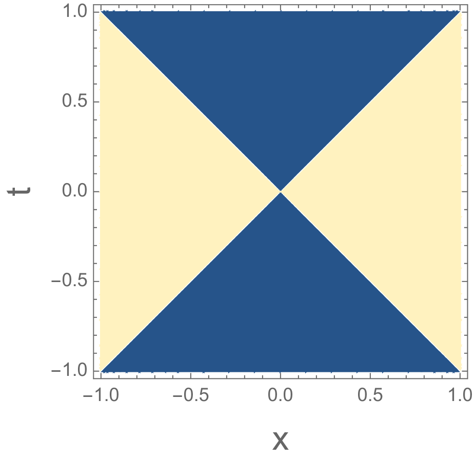
(b) Two bubble walls colliding at the origin

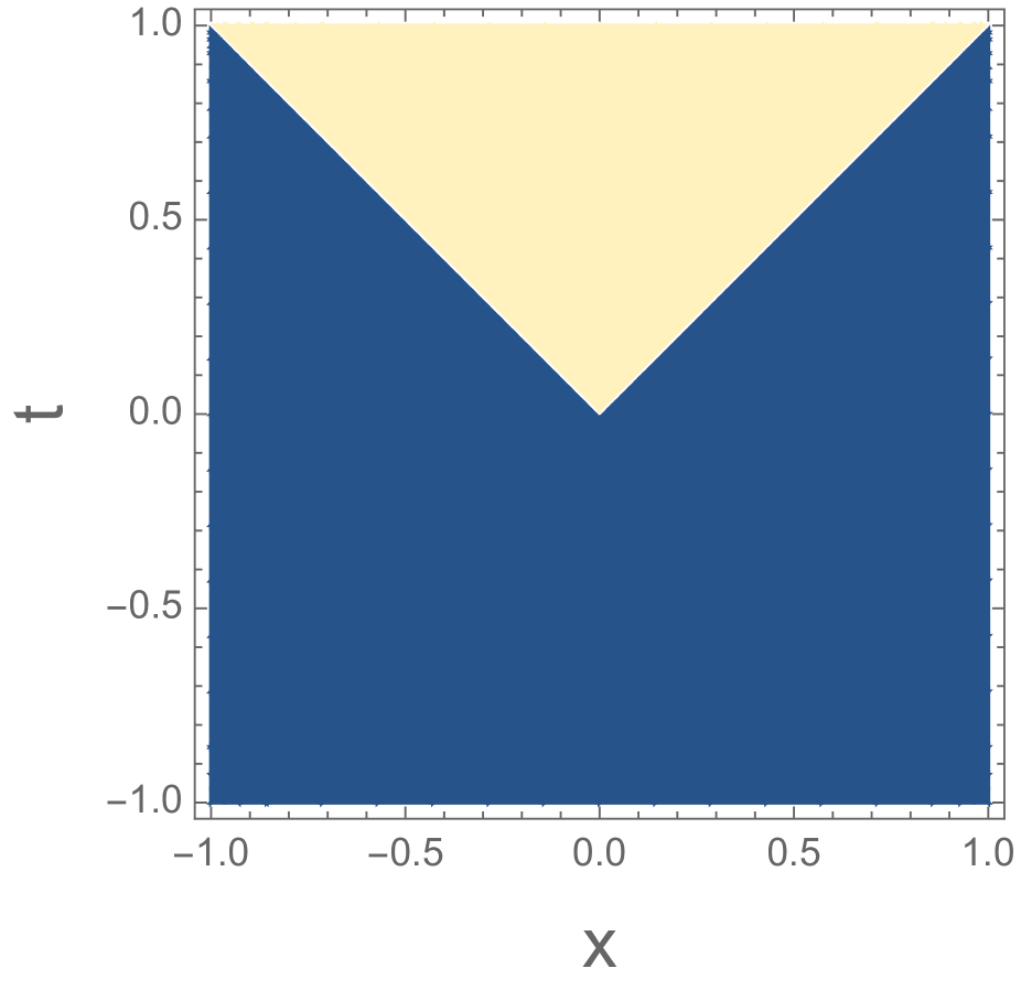
(c) Single bubble expanding out from the origin

Figure 1: Spacetime evolution of some simple field configurations of planar thin-walled bubbles, plotted for wall speed $v_{w}\approx 1$. The yellow (light) and blue (dark) regions corresponds to the true and false vacua respectively.

(c) Single expanding bubble:

Next, consider a single bubble that starts as a point (at the origin) and expands outwards at constant speed $v_{\mathrm{w}}$ (see Fig. 1(c) ). The field configuration in this case can be written as

$$\phi(x,t)=v_{\phi}\,\Theta(v_{\mathrm{w}}\,t-|x|)\,$$ (22)

and yields the Fourier transform

$$\tilde{\phi}(k,\omega)=\frac{2\,v_{\phi}}{\omega^{2}-k^{2}\,v_{\mathrm{w}}^{2}}\,.$$ (23)

Incredibly, this is the same as the Fourier transform for the case of an elastic bubble collision, Eq. (21), with half the amplitude (originating from the fact that the scalar field only changes in half the plane in this case). This makes it clear that the mode excitations in Eq. (21) originate purely from the relative motion of the two bubble walls, and do not receive any contributions from the collision itself.

III.3 Realistic Cases

The above simple cases capture the contributions from the bubble walls moving relative to each other, but not from the scalar field excitations and oscillations that occur after bubble collisions in any realistic setup. Here, we summarize the results from the literature for the efficiency factor $f(\chi)$ for realistic cases that incorporates these effects.

Ref [69] presents analytic formulae in the idealized cases where the collision between two bubbles is either perfectly elastic or totally inelastic. For a perfectly elastic collision, where the walls bounce back perfectly with no energy dissipation in scalar oscillations, the efficiency factor is [69]

$$f_{\mathrm{PE}}(\chi)=\frac{16v_{\phi}^{2}}{\chi^{2}}\,\text{Log}\left[\frac{2(\gamma_{w}/l_{w})^{2}-\chi+2(\gamma_{w}/l_{w})\sqrt{(\gamma_{w}/l_{w})^{2}-\chi}}{\chi}\right]\,.$$ (24)

For a totally inelastic collision, where the collision results in the bubble walls completely dissociating and all the energy going into scalar field oscillations, the factor is [69]

$$f_{\mathrm{TI}}(\chi)=\frac{4v_{\phi}^{2}m_{t}^{4}}{\chi^{2}\left[(\chi-m_{t}^{2})^{2}+m_{t}^{6}\left(\frac{l_{w}}{\gamma_{w}}\right)^{2}\right]}\mathrm{Log}\left[\frac{2\left(\frac{\gamma_{w}}{l_{w}}\right)^{2}+\chi+2\frac{\gamma_{w}}{l_{w}}\sqrt{\left(\frac{\gamma_{w}}{l_{w}}\right)^{2}+\chi}}{\chi}\right]\,,$$ (25)

where $m_{t}$ is the scalar mass in the true minimum.

While the above represent two idealized limits, a realistic collision consists of some combination of propagating walls and scalar field oscillations, determined by the details of the scalar potential. Ref [74] studied such realistic collisions numerically, and found the following fit functions for the efficiency factor for elastic and inelastic collisions:

$$f_{\text{elastic}}(\chi)=f_{\mathrm{PE}}(\chi)+\frac{v_{\phi}^{2}L_{p}^{2}}{15m_{\mathrm{t}}^{2}}\exp{\left(\frac{-(\chi-m_{\mathrm{t}}^{2}+12m_{\mathrm{t}}/L_{p})^{2}}{440\,m_{\mathrm{t}}^{2}/L_{p}^{2}}\right)}\qquad\text{(elastic collisions)}$$ (26)

$$f_{\text{inelastic}}(\chi)=f_{\mathrm{PE}}(\chi)+\frac{v_{\phi}^{2}L_{p}^{2}}{4m_{\mathrm{f}}^{2}}\exp{\left(\frac{-(\chi-m_{\mathrm{f}}^{2}+31m_{\mathrm{f}}/L_{p})^{2}}{650\,m_{\mathrm{f}}^{2}/L_{p}^{2}}\right)}\qquad\text{(inelastic collisions)}$$ (27)

Here, $f_{\mathrm{PE}}$ is the efficiency factor for a perfectly elastic collision as given in Eq. (24), and $m_{t},\,m_{f}$ are the scalar masses in the true and false vacua respectively. $L_{p}=\text{min}(R_{*},\Gamma^{-1})$, where $\Gamma$ is the decay rate of the scalar and $R_{*}$ is the typical bubble size at collision, provides a measure of the extent to which scalar oscillations propagate in spacetime.

It is important to keep in mind that the above results are only applicable within a finite range of values of $\chi$, confined by physical scales in the setup. In the ultraviolet (UV), the results are not applicable for distances smaller than the boosted wall thickness $l_{w}/\gamma_{w}$, as effects related to the finite width of the bubble wall, which are not taken into account, become important. Likewise, the infrared (IR) cutoff is given by the inverse of the bubble wall radius $R_{*}^{-1}$; at physical scales larger than this, the existence of multiple bubbles should be taken into account.

It is worth mentioning here that the above formulae only include the expansion and collision phases of the FOPT, but ignore the bubble nucleation process. In practice, this is because the scale of bubble nucleation is much smaller than the scale of the above studies, and cannot be properly resolved in the numerical approaches. While this shortcoming can be rectified, since the bubble nucleation phase is also amenable to the homogeneous approximation and analytic treatment, we can choose to consider the nucleation phase separately (see Sec. II.2).

III.4 Understanding Particle Production

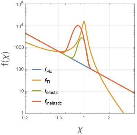
Figure 2: Efficiency factor for particle production $f(\chi)$ in the four cases discussed in Sec. III.3. For this plot, all masses are set to $v_{\phi}$, and we use $l_{w}=10/v_{\phi},\,\gamma_{w}=200,$ and $L_{p}=200/v_{\phi}$. The axes ($f(\chi)$ and $\chi$ are plotted in appropriate units of $v_{\phi}$.

The four functions for the efficiency factor from the previous subsection are plotted in Fig. 2 (the differences between the analytic formulae and numerical fits are discussed in detail in [74]). These results, along with the results for the Fourier transforms for the simple cases from Sec. III.2, enable us to gain insight into the process of particle production.

Note that both the analytic and numerical fit formulae consist of a combination of a power law and a peak in the spectrum. In all cases (except the totally inelastic case), the power law follows the form $f(\chi)\sim f_{PE}(\chi)\sim\chi^{-2}$ up to a logarithmic factor. This form of $f_{\text{PE}}$ in the perfectly elastic collision limit follows from the Fourier transform in Eq. (21). From the simple cases examined above, it becomes clear that this contribution comes from the relative motion of the two bubble walls, and receives no contribution from the collision itself (recall that the Fourier transform of a single expanding bubble, which features identical motion of the walls without any collision, gives the same Fourier transform (Eq. (23)) ). This interpretation is further supported by the observation that the result for the totally inelastic case Eq. (25), which only considers the field configuration after collision, i.e. after the bubble walls have disappeared, does not feature this power law. In particular, from considering the geometry of the setup, a mode excitation with four-momentum $\sqrt{\chi}=p$ corresponds to the configuration where the two walls are at a distance $p^{-1}$ apart, providing a physical explanation of why the background field experiences an excitation at this scale.

The above discussion implies that the configuration of two approaching bubble walls is already responsible for half of the contribution to $f_{\text{PE}}$. This pre-collision contribution is therefore universal to all FOPTs, independent of the post-collision dynamics of the field configuration. It is worth emphasizing that this feature of particle production is in stark contrast to the production of gravitational waves. It is well known that GWs correspond to transverse, traceless excitations of the metric, which cannot be sourced by spherically symmetric bubble walls, i.e. by the expansion of bubbles before collision; therefore GW spectra from bubble collisions do not feature this falling power law across a large range of scales. No such restrictions exist for particle production, which can thus take place even before bubbles collide, resulting in this power law component in the spectrum.

The plots in Fig. 2 also show a peak in the spectrum, at the effective mass of the scalar field in the true (false) vacuum for inelastic (elastic) collisions. This component originates from oscillations of the background field around the relevant minimum after the field gets excited to unstable values as a result of the bubble collision. Crucially, note that this component is clustered around the scalar field mass, and does not contribute at higher $\chi$. This is particularly evident from the result for the totally inelastic case, which only considers post-collision contributions (i.e. no bubble walls) (see Eq. (25) and Fig. 2), and does not have a $\chi^{-2}$ tail at $\chi>m_{t}^{2}$.

This leads us to an important observation: the production of particles with masses or energies much higher than the scale of the phase transition, i.e. $E\gg v_{\phi},m_{t},m_{f}$, occurs not as a consequence of the collision between energetic bubble walls, but from the relative motion of the two walls when they are at a distance $E^{-1}$ apart. In addition to providing insight into the physics of the process, this observation will also be crucial for a proper calculation of particle production, as we will see in the next section.

IV Particle Physics Aspects

The earlier sections have primarily focused on the spacetime configuration of the background field. This section is devoted to a discussion of some particle physics aspects relevant for particle production.

IV.1 Non-universality of Particle Interactions and Masses

During a FOPT, both the true and false vacua coexist simultaneously in different parts of space, and the Fourier transform gives the distribution of excitations over this mixed configuration. The nature of particle interactions, as well as particle masses, are generally different in the two vacua. Therefore, a crucial question arises: for the purposes of particle production – in particular, the calculation of matrix elements in Eq. (15) relevant for the decay of the excitations – which vacuum is the correct one to use? Previous papers [72, 73, 69] simply chose interactions and masses in the true vacuum, assuming particle production to be a post-collision phenomenon. However, as we will see below, the scenario is more subtle and requires greater care.

For concreteness, consider again a scalar field $\psi$ that couples to the background scalar field $\phi$ driving the phase transition via

$$-\Delta\mathcal{L}_{\psi}=\frac{\lambda}{2}\phi^{2}\psi^{2}+\frac{1}{2}m_{0}^{2}\psi^{2},$$ (28)

where $\lambda$ is a dimensionless coupling and $m_{0}$ is a bare mass for $\psi$, which we include for generality. Again, let us take the scalar field vev to be $0$ and $v_{\phi}$ in the false and true vacua respectively. In the false vacuum, $\psi$ therefore only interacts with $\phi$ via a quartic term; consequently, an off-shell $\phi$ excitation can only decay into a three body final state $\phi^{*}\to\phi\psi\psi$. Note that the $\psi$ mass in the false vacuum is $m_{0}$.

In the true vacuum, one can also replace the $\phi$ field with its nonzero vev, so we have

$$-\Delta\mathcal{L}_{\psi\,(true)}=\frac{\lambda}{2}\phi^{2}\psi^{2}+\lambda v_{\phi}\phi\psi^{2}+\frac{1}{2}(\lambda v_{\phi}^{2}+m_{0}^{2})\psi^{2},$$ (29)

Thus, in the true vacuum $\psi$ now interacts with $\phi$ via both a quartic and cubic term, so that the background scalar excitations can decay via $\phi^{*}\to\psi\psi$ in addition to the previously encountered $\phi^{*}\to\phi\psi\psi$. The imaginary part of the 2-point 1PI Green’s function for these two cases are given by

$$\mathrm{Im}\left(\tilde{\Gamma}^{(2)}(\chi)\right)_{\phi^{*}\to\psi\psi} = \frac{\lambda^{2}v_{\phi}^{2}}{8\pi}\sqrt{1-\frac{4m_{\psi}^{2}}{\chi}}\,\Theta[\,\chi-(2m_{\psi})^{2}]\,,$$

$$\mathrm{Im}\left(\tilde{\Gamma}^{(2)}(\chi)\right)_{\phi^{*}\to\phi\psi\psi} = \frac{\lambda^{2}\chi}{512\pi^{3}}\sqrt{1-\frac{(m_{\phi}+2m_{\psi})^{2}}{\chi}}\,\Theta[\,\chi-(m_{\phi}+2m_{\psi})^{2}].$$ (30)

Moreover, in the true vacuum, the $\psi$ mass is $m_{\psi}^{2}=m_{0}^{2}+\lambda v_{\phi}^{2}$.

The $\psi$ interactions as well as mass are therefore vacuum dependent, and it becomes important to determine which vacuum is relevant for particle production. Note that this subtlety does not arise for the calculation of gravitational waves production, since the graviton coupling is universal.

Resolving this for particle production necessitates understanding where the production process is taking place. There are three possibilities:

1. Inside the bubbles of true vacuum as they nucleate and expand. In this case, the interactions and masses in the true vacuum are the correct ones to use.

2. In the space in between expanding bubbles as the bubbles approach each other before they collide. Here, the interactions and masses in the false vacuum are the relevant ones.

3. In the region with scalar waves after the bubble walls collide. This corresponds to the true vacuum for inelastic collision. For elastic collisions, however, this corresponds to the false vacuum, which is re-established, with the bubble walls bouncing back and receding from each other before colliding repeatedly.

We begin the construction of a solution with the observation that particle production is a local process. A particle with mass $m$ has a typical physical scale associated with it: its Compton wavelength $\sim m^{-1}$; it can only be produced by dynamics at length scales smaller than this. Recall that contributions to the efficiency factor $f(\chi)$ at scale $\sqrt{\chi}$ correspond to scalar field dynamics over a length scale $1/\sqrt{\chi}$, e.g. when two bubble walls are approaching or receding from each other at this distance. Since bubbles of true vacuum nucleate with some critical radius $R_{c}\gg l_{w}\sim v_{\phi}^{-1}$ in the thin wall approximation, contribution (1) above can thus only produce particles with mass $m<R_{c}^{-1}$ during the expansion phase of the bubble (the nucleation contribution is calculated separately as described in Sec. II.2). Exciting particles with $m>R_{c}^{-1}$ during the expansion phase requires two bubble walls to be within a distance smaller than $R_{c}$, which can occur for both (2) and (3) above. We are therefore led to the following prescription for the choice of vacuum for calculating particle production

• Particles with mass $m\!>\!R_{c}^{-1}$ in elastic collisions: use interactions in the false vacuum, with efficiency factor $f_{\text{elastic}}$ given in Eq. (26), as these particles are produced in the region between the two bubble walls.

• Particles with mass $m\!>\!R_{c}^{-1}$ in inelastic collisions: production occurs in both false and true vacua (before and after the collision respectively), corresponding to cases (2) and (3) above, thus one needs to sum the two contributions. The contribution before collision can be captured by using $\frac{1}{2}f_{PE}$ with false vacuum interactions, whereas the corresponding contribution after collision is given by $f_{\text{inelastic}}-\frac{1}{2}f_{PE}$ with true vacuum interactions.

• Particles with mass $R_{*}^{-1}\!<\!m\!<\!R_{c}^{-1}$: This scenario is more complicated, since production can occur through bubble wall dynamics as well as scalar oscillations, and both inside and outside the bubbles. For $\chi\!>\!R_{c}^{-2}$, we can follow the above prescriptions. For smaller values $\chi\!<\!R_{c}^{-2}$, all three configurations $(1,2,3)$ listed above can contribute. The trick is to identify that all three configurations are realized for the same amount of time, thus all three must be included with equal weight. Depending on whether the collision is elastic or inelastic, the false or true vacuum becomes twice as prominent in this regime. It should be noted, though, that in general $m_{f}\sim v_{\phi}>R_{c}^{-1}$, hence the false vacuum configuration, which must decay as $\phi^{*}\to\phi\psi\psi$, is generally kinematically forbidden in the $\chi<R_{c}^{-2}$ region, and only the true vacuum contribution is possible. Additionally, note that the above formulae for the efficiency factor break down below the IR cutoff $\chi=R_{*}^{-2}$, hence cannot be used to calculate the production of particles with masses below this cutoff.

The mass $m$ of the particle being produced is also vacuum dependent. In principle, one must also use the mass corresponding to the vacuum of choice above. However, note that if the particle is massless in the unbroken vacuum, as can occur in many realistic scenarios, then its Compton wavelength is infinite. Even it is has a small mass, its Compton wavelength may extend beyond the physical size of the false vacuum region, into the true vacuum (or vice-versa). In such cases, it appears plausible that the true vacuum mass of the particle should be used for the calculation. The form of the interaction, on the other hand, should correspond to the vacuum where the excitation is localized, as described above.

The above prescription, while not rigorous, nevertheless captures many aspects of the underlying physics giving rise to particle production.

IV.2 Non-perturbative Effects

So far, we have not considered the possibility of nonperturbative, resonant enhancement of particle production. Ref. [72] suggested that reaheating after FOPTs should occur in essentially the same way as in inflation. It is well known that nonperturbative processes such as tachyonic instability and parametric resonance can be important in such cases, resulting in explosive particle production, depending on the details of the scalar field dynamics in such cases [90, 91, 92, 93, 94, 95, 96]. Furthermore, Ref. [97] found that parametric resonance can lead to very efficient particle production at bubble collisions. However, all of the standard studies of such resonant effects [90, 91, 92, 93, 94, 95, 96] are performed under the assumption that the background field evolution is spatially homogeneous. The study of bubble collisions in Ref. [97] was also performed with this setup, i.e. neglecting spatial gradient terms in the equation of motion. In this subsection, we qualitatively discuss the relevance of such resonant effects for particle production from FOPTs considering the highly inhomogeneous nature of the process. Here we will only discuss the case of tachyonic instability; the main arguments and conclusions apply analogously to the case of parametric resonance.

Consider again the Klein Gordon equation for a scalar field $\psi$

$$(\partial_{t}^{2}-\partial_{x}^{2}+m_{\text{eff},\psi}^{2}(x,t))\,\psi(t,x)=0\,,$$ (31)

where the effective mass $m_{\text{eff},\psi}$ can receive contributions from the background field undergoing the phase transition. In the homogeneous limit, one can decompose the $\phi$ field into modes of definite momenta. If $m_{\text{eff},\psi}^{2}(t)<0$, modes with momenta $k<|m_{\text{eff},\psi}|$ experience tachyonic instability and have an exponentially growing solution

$$\psi_{k}(t)\propto\,\mathrm{exp}\,\left[\sqrt{m_{\text{eff},\psi}^{2}(t)-k^{2}}\,t\,\right]\,.$$ (32)

This results in a rapid coherent growth of particle number.

When the setup is spatially inhomogeneous, the above result receives several modifications. First, the spatial derivative term in Eq. (31) can become large, and it is well known that spatial derivatives have the effect of countering time derivatives, suppressing the rapid time evolution of the field. Furthermore, assuming the mass becomes tachyonic due to the effects of the background field dynamics, $m_{\text{eff},\psi}^{2}(x,t)<0$ now only holds in finite regions of space, corresponding to the length scale of the boosted bubble walls or the scalar field oscillation scale $v_{\phi}\sim m_{t,f}$. As a result, Eq. (32) is now only applicable for this, or smaller, length scale, i.e. for $k>v_{\phi}$. However, if the tachyonic mass is an outcome of the background field dynamics, it is plausible to assume $|m_{\text{eff},\psi}|<v_{\phi}$. Thus we see that the finite spatial extent of the dynamics tends to affect precisely the modes $k<|m_{\text{eff},\psi}|$ that could grow tachyonically. Moreover, since such particle production now only takes in a finite region of space, the produced particles no longer collect coherently at their production point but diffuse out in space. Such dissipation occurs over a timescale given by the scale of the inhomogeneity, $t\sim v_{\phi}^{-1}$. This timescale is shorter than the timescale over which the exponential growth of particle number occurs in Eq. (32), $t\sim m_{\text{eff},\psi}^{-1}$, which provides another argument for the suppression of tachyonic growth in such inhomogeneous configurations.

Similar arguments apply to parametric resonance. The point, in essence, is that resonant processes such as tachyonic instability and parametric resonance require a coherent setting that seeds the growth of particle number. Such coherence is lost in FOPTs due to the inhomogeneous nature of the process: the mass term is only coherent over spatial distances $\sim v_{\phi}^{-1}$, and dissipation of particle number over space due to particle production in localized regions prevents a coherent growth of particle number beyond timescales $\sim v_{\phi}^{-1}$. Because of such factors, it is unlikely that such resonant processes can be very effective for particle production from FOPTs. It will be interesting to perform explicit (likely numerical) calculations incorporating such inhomogeneities to understand whether this is indeed the case.

V Summary

This paper discusses various aspects related to particle production from the dynamics of the background scalar field in a first order phase transition (FOPT), providing improved conceptual understanding of the underlying physics of the process beyond what currently exists in the literature. The main findings of this paper are summarized below:

• The process of bubble nucleation creates particles that couple to the background field. This can be estimated using the same calculation as particle production out of vacuum in a homogeneous transition, and is given by Eq. (11). The number density of produced particles is parametrically $\sim l_{w}^{-3}(R_{c}/R_{*})^{3}$. The physical scale of the process is $l_{w}^{-1}$, the inverse wall thickness, which also parameterizes the timescale of bubble nucleation; the $(R_{c}/R_{*})^{3}$ factor accounts for diffusion of the particles from the bubble nucleation site to all space.

• Particle production from the bubble expansion and collision phases of the transition are captured by Eq. (17), (16), with the efficiency factor $f(\chi)$ given by Eq. (26) for elastic collisions and Eq. (27) for inelastic collisions. $f(\chi)$ consists of a power law component $f(\chi)\sim\chi^{-2}$, which originates from the relative motion of bubble walls in the expansion phase, and a peak centered around the effective mass of the scalar, which comes from scalar field oscillations following bubble collisions.

• From analyzing the Fourier transforms of realistic collision configurations relative to a few simple cases, it was shown that heavy particles are produced from the configuration of bubble walls moving relative to each other at a distance equal to the Compton wavelength of the particle, rather than from bubble collisions. The relative motion of bubble walls is crucial; it was shown that a single propagating wall cannot produce particles (see Sec. II.3).

• Particle interactions and masses are not universal, and take different forms in the two vacua, which coexist during a FOPT. Through considerations of the location of particle production for various cases, Sec. IV.1 provided prescriptions for choosing the correct vacuum to perform particle production calculations.

• Implications of the inhomogeneous nature of the process for nonperturbative, resonant effects were examined in Sec. IV.2. Since masses are not coherent over scales larger than $v_{\phi}^{-1}$, and particles diffuse out from the localized production points over a timescale $v_{\phi}^{-1}$, preventing a coherent buildup of particle number, such processes are likely suppressed and irrelevant for FOPTs.

It is worth repeating the two crucial differences between particle production and the production of gravitational waves (GWs) highlighted in this work: (1) the configuration of expanding bubbles before collision can already produce particles (giving rise to the power law component in the efficiency factor spectrum), whereas no GWs are produced in this phase due to the transverse-traceless requirement, and (2) the non-universal nature of particle interactions and couplings in different vacua necessitates greater caution in choosing the appropriate vacuum for particle production calculations, whereas this ambiguity is absent for GW production due the universal nature of the gravitational coupling.

The improved understanding of the particle production process provided by this paper invites further investigation into various related matters. The prescription for choosing the correct vacuum provided here, as well as the arguments for the inefficiency of nonperturbative processes, are based on simple intuitive arguments, but could (and should) be further sharpened with more rigorous calculations. The effects of particle production on bubble dynamics and the subsequent production of gravitational waves also merits further study. Likewise, such particle production processes could be of relevance for various nonthermal beyond the Standard Model (BSM) applications, such as baryogenesis and dark matter. Such BSM applications, and additional subtleties related to the application of the particle production process to specific BSM models, will be discussed in future work [98].

Appendix A Particle Production from a Single Propagating Bubble Wall

The goal of this appendix is to understand particle production using the standard Bogoliubov transformation approach for a scalar $\psi$ that follows the Klein Gordon equation from Eq. 12:

$$\left(-\frac{\partial^{2}}{\partial t^{2}}+\frac{\partial^{2}}{\partial x^{2}}\right)\psi(t,x)=\frac{m_{\psi}^{2}}{4}\left(1-\text{tanh}\left(\frac{v_{w}t-x}{l_{w}}\right)\right)^{2}\psi(t,x)\,.$$ (33)

If the field $\psi$ is in its vacuum state in the false vacuum, it can be written as a collection of harmonic oscillators with negative frequencies $\sim\int\frac{dp}{\sqrt{2E}}\,e^{-i\omega t+ipx}$, where $\omega$ is determined via the standard dispersion relation $w^{2}=p^{2}+m^{2}$. Following the standard approach of Bogoliubov transformations, our goal is to expand the late time asymptotic solution $\psi(vt>x)$ in terms of its mode functions $\psi_{p}$, expressing the mode functions in the form

$$\psi_{p}\sim\frac{1}{\sqrt{2E}}\,(\alpha_{p}\,e^{-i\omega t}+\beta_{p}\,e^{i\omega t})$$ (34)

The positive frequency modes can be interpreted as particles, with the number density of particles produced (with momentum p) given by the square of the Bogoliubov coefficient in the above expansion, $n_{p}=|\beta_{p}|^{2}.$

To obtain this solution, note that the mass term in Eq. 33 depends on both variables $t$ and $x$. Hence we first change variables to eliminate this double dependence by switching to the new coordinates $(x_{1},x_{2})$ given by

$$x_{1}=\frac{1}{\sqrt{1+v_{w}^{2}}}(v_{w}t-x),~{}~{}~{}x_{2}=\frac{1}{\sqrt{1+v_{w}^{2}}}(t+v_{w}x)\,.$$ (35)

With these new coordinates, we can use the relation

$$g^{\prime}_{\mu v_{\phi}}(x^{\prime})=\frac{\partial x^{\rho}}{\partial x^{\prime\mu}}\frac{\partial x^{\sigma}}{\partial x^{\prime v}_{\phi}}g_{\rho\sigma}(x)$$ (36)

to rewrite the general KG equation

$$(g^{\alpha\beta}\partial_{\alpha}\partial_{\beta}-m^{2})\phi=0$$ (37)

as

$$\left[\,\left(\frac{1-v_{w}^{2}}{1+v_{w}^{2}}\right)\left(-\frac{\partial^{2}}{\partial x_{2}^{2}}+\frac{\partial^{2}}{\partial x_{1}^{2}}\right)-\frac{4v_{w}}{1+v_{w}^{2}}\frac{\partial}{\partial x_{1}}\frac{\partial}{\partial x_{1}}\right]\phi(t,x)={m_{\psi}^{2}(x_{1})}\phi(t,x)\,,$$ (38)

where the mass term now only varies along $x_{1}$:

$$m_{\psi}^{2}(x_{1})=\frac{m_{\psi}^{2}}{4}\left(1-\text{tanh}\left(\frac{\sqrt{1+v_{w}^{2}}\,x_{1}}{l_{w}}\right)\right)^{2}\,.$$ (39)

The physics is now invariant under translations along $x_{2}$, hence its conjugate momentum $p_{2}$ is a conserved quantity. We can therefore expand the field $\psi$ in terms of its $p_{2}$ modes, and solve the modified KG equation Eq. 38 mode-by-mode (note that such momentum decomposition is only justified if the corresponding momentum is conserved, hence this choice of coordinates) to construct our solution. For each $p_{2}$ mode, Eq. 38 gives

$$\left(\frac{\partial^{2}}{\partial x_{1}^{2}}-\frac{4iv_{w}p_{2}}{1-v_{w}^{2}}\frac{\partial}{\partial x_{1}}\right)\phi(x_{1})=\left[\frac{1+v_{w}^{2}}{1-v_{w}^{2}}{m(x_{1})^{2}}-p_{2}^{2}\right]\phi(x_{1})\,.$$ (40)

We anticipate being able to write the asymptotic form of the solution in terms of a superposition of plane waves $\sim e^{ip_{1}x_{1}+ip_{2}x_{2}}$. Recall that the initial vacuum state configuration is a superposition of negative frequency modes $\sim\int\frac{dp}{\sqrt{2E}}\,e^{-i\omega t+ipx}$. Rewriting these in terms of the new coordinates, we get

$$e^{-i\omega t+ipx}=\text{exp}\left[-\frac{\omega v_{w}+p}{\sqrt{1+v_{w}^{2}}}x_{1}-\frac{\omega-pv_{w}}{\sqrt{1+v_{w}^{2}}}x_{2}\right]$$ (41)

The conjugate of $x_{2}$, which corresponds to a conserved quantity, is

$$p_{2}=-\frac{\omega-pv_{w}}{\sqrt{1+v_{w}^{2}}}=-\frac{|p|-pv_{w}}{\sqrt{1+v_{w}^{2}}}\,,$$ (42)

where we have used $\omega=|p|$ for the initial state since $\psi$ is initially massless. Note that there is a degeneracy: two different values of p (one positive, one negative) map on to the same value of $p_{2}$. The conjugate of the other coordinate $x_{1}$ is given by

$$p_{1}=-\frac{\omega v_{w}+p}{\sqrt{1+v_{w}^{2}}}\,.$$ (43)

This quantity is not conserved but changes across across the bubble wall.

Next, we examine the dispersion relation in our new coordinates. For a plane wave $\sim e^{ip_{1}x_{1}+ip_{2}x_{2}}$, Eq. 38 enforces the following dispersion relation between the conjugate momenta:

$$p_{1}^{2}-p_{2}^{2}-\frac{4v_{w}}{1-v_{w}^{2}}p_{1}p_{2}+m_{\psi}^{2}\frac{1+v_{w}^{2}}{1-v_{w}^{2}}=0.$$ (44)

This can be rewritten as a solution for $p_{1}$ in terms of $p_{2}$:

$$p_{1}=\frac{2v_{w}p_{2}}{1-v_{w}^{2}}\pm\sqrt{\frac{p_{2}^{2}(1+v_{w}^{2})^{2}-m_{\psi}^{2}(1-v_{w}^{4})}{(1-v_{w}^{2})^{2}}}\,.$$ (45)

This represents the mixing between modes due to the change in mass across the bubble wall. The two values correspond to the transmitted and reflected parts of the plane wave of conjugate momentum mode $p_{2}$ when it encounters the bubble wall, and the final asymptotic form can be written as a superposition of these two parts for each mode.

Next, we rewrite the general asymptotic form of the plane wave in the new coordinates in terms of the physical space and time coordinates $x,t$:

$$e^{ip_{1}x_{1}+ip_{2}x_{2}}\sim\text{exp}\left[\frac{p_{1}v_{w}+p_{2}}{\sqrt{1+v_{w}^{2}}}t+\frac{p_{2}v_{w}+p_{1}}{\sqrt{1+v_{w}^{2}}}x\right]\,.$$ (46)

We are interested in the coefficient of the time coordinate in the exponential, $p_{1}v_{w}+p_{2}$, at late times. In particular, since particles correspond to positive frequencies, we are interested in scenarios where this coefficient can be positive, i.e.

$$\frac{p_{1}v_{w}+p_{2}}{\sqrt{1+v_{w}^{2}}}>0\,.$$ (47)

Substituting in $p_{1}$ from Eq. 45, this condition can be written as

$$p_{2}\,\frac{1+v_{w}^{2}}{1-v_{w}^{2}}\pm v_{w}\sqrt{\frac{p_{2}^{2}(1+v_{w}^{2})-m_{\psi}^{2}(1-v_{w}^{4})}{(1-v_{w}^{2})^{2}}}>0\,.$$ (48)

The two values, again, correspond to the frequencies of the transmitted and reflected parts of the incoming plane wave.

From Eq. 42, we have $p_{2}=-({|p|-pv_{w}})/{\sqrt{1+v_{w}^{2}}}$. If $p>0$, we have $p_{2}=-p(1-v_{w})/\sqrt{1+v_{w}^{2}}<0$ for $v_{w}<1$. Likewise, if $p<0$, then $p_{2}=p(1+v_{w})/\sqrt{1+v_{w}^{2}}<0$ again. Thus, we conclude that the first term in Eq. 48 is always negative for $v_{w}<1$ for $p_{2}$ given by Eq. 42, i.e. any component of the initial vacuum (negative frequency) state. Thus, the condition in Eq. 48 can only be satisfied if the second term (featuring the square root) is bigger than the first term, and for the positive sign. The condition for this, after a bit of algebra, is

$$p_{2}^{2}(v_{w}^{4}-1)>m_{\psi}^{2}(1-v_{w}^{2})\,.$$ (49)

Note that the above calcuation and result is independent of the exact form of the mass term in Eq. 33, and remains applicable as long as the change of coordinates restricts the mass variation to a single coordinate.

References

- Hogan [1983] C. J. Hogan, NUCLEATION OF COSMOLOGICAL PHASE TRANSITIONS, Phys. Lett. B 133, 172 (1983).
- Witten [1984] E. Witten, Cosmic Separation of Phases, Phys. Rev. D 30, 272 (1984).
- Hogan [1986] C. J. Hogan, Gravitational radiation from cosmological phase transitions, Mon. Not. Roy. Astron. Soc. 218, 629 (1986).
- Kosowsky et al. [1992a] A. Kosowsky, M. S. Turner, and R. Watkins, Gravitational radiation from colliding vacuum bubbles, Phys. Rev. D 45, 4514 (1992a).
- Kosowsky et al. [1992b] A. Kosowsky, M. S. Turner, and R. Watkins, Gravitational waves from first order cosmological phase transitions, Phys. Rev. Lett. 69, 2026 (1992b).
- Kosowsky and Turner [1993] A. Kosowsky and M. S. Turner, Gravitational radiation from colliding vacuum bubbles: envelope approximation to many bubble collisions, Phys. Rev. D 47, 4372 (1993), arXiv:astro-ph/9211004 .
- Kamionkowski et al. [1994] M. Kamionkowski, A. Kosowsky, and M. S. Turner, Gravitational radiation from first order phase transitions, Phys. Rev. D 49, 2837 (1994), arXiv:astro-ph/9310044 .
- Guth [1981] A. H. Guth, Inflationary universe: A possible solution to the horizon and flatness problems, Phys. Rev. D 23, 347 (1981).
- La and Steinhardt [1989] D. La and P. J. Steinhardt, Extended inflationary cosmology, Phys. Rev. Lett. 62, 376 (1989).
- Grojean and Servant [2007] C. Grojean and G. Servant, Gravitational Waves from Phase Transitions at the Electroweak Scale and Beyond, Phys. Rev. D75, 043507 (2007), arXiv:hep-ph/0607107 [hep-ph] .
- Caprini et al. [2016] C. Caprini et al., Science with the space-based interferometer eLISA. II: Gravitational waves from cosmological phase transitions, JCAP 1604, 001, arXiv:1512.06239 [astro-ph.CO] .
- Caprini and Figueroa [2018] C. Caprini and D. G. Figueroa, Cosmological Backgrounds of Gravitational Waves, Class. Quant. Grav. 35, 163001 (2018), arXiv:1801.04268 [astro-ph.CO] .
- Caprini et al. [2020] C. Caprini et al., Detecting gravitational waves from cosmological phase transitions with LISA: an update, JCAP 2003, 024, arXiv:1910.13125 [astro-ph.CO] .
- Athron et al. [2023] P. Athron, C. Balázs, A. Fowlie, L. Morris, and L. Wu, Cosmological phase transitions: from perturbative particle physics to gravitational waves, (2023), arXiv:2305.02357 [hep-ph] .
- Schwaller [2015] P. Schwaller, Gravitational Waves from a Dark Phase Transition, Phys. Rev. Lett. 115, 181101 (2015), arXiv:1504.07263 [hep-ph] .
- Jaeckel et al. [2016] J. Jaeckel, V. V. Khoze, and M. Spannowsky, Hearing the signal of dark sectors with gravitational wave detectors, Phys. Rev. D 94, 103519 (2016), arXiv:1602.03901 [hep-ph] .
- Dev and Mazumdar [2016] P. S. B. Dev and A. Mazumdar, Probing the Scale of New Physics by Advanced LIGO/VIRGO, Phys. Rev. D 93, 104001 (2016), arXiv:1602.04203 [hep-ph] .
- Baldes [2017] I. Baldes, Gravitational waves from the asymmetric-dark-matter generating phase transition, JCAP 05, 028, arXiv:1702.02117 [hep-ph] .
- Tsumura et al. [2017] K. Tsumura, M. Yamada, and Y. Yamaguchi, Gravitational wave from dark sector with dark pion, JCAP 07, 044, arXiv:1704.00219 [hep-ph] .
- Okada and Seto [2018] N. Okada and O. Seto, Probing the seesaw scale with gravitational waves, Phys. Rev. D 98, 063532 (2018), arXiv:1807.00336 [hep-ph] .
- Croon et al. [2018] D. Croon, V. Sanz, and G. White, Model Discrimination in Gravitational Wave spectra from Dark Phase Transitions, JHEP 08, 203, arXiv:1806.02332 [hep-ph] .
- Baldes and Garcia-Cely [2019] I. Baldes and C. Garcia-Cely, Strong gravitational radiation from a simple dark matter model, JHEP 05, 190, arXiv:1809.01198 [hep-ph] .
- Prokopec et al. [2019] T. Prokopec, J. Rezacek, and B. Świeżewska, Gravitational waves from conformal symmetry breaking, JCAP 02, 009, arXiv:1809.11129 [hep-ph] .
- Bai et al. [2019] Y. Bai, A. J. Long, and S. Lu, Dark Quark Nuggets, Phys. Rev. D 99, 055047 (2019), arXiv:1810.04360 [hep-ph] .
- Breitbach et al. [2019] M. Breitbach, J. Kopp, E. Madge, T. Opferkuch, and P. Schwaller, Dark, Cold, and Noisy: Constraining Secluded Hidden Sectors with Gravitational Waves, JCAP 07, 007, arXiv:1811.11175 [hep-ph] .
- Fairbairn et al. [2019] M. Fairbairn, E. Hardy, and A. Wickens, Hearing without seeing: gravitational waves from hot and cold hidden sectors, JHEP 07, 044, arXiv:1901.11038 [hep-ph] .
- Helmboldt et al. [2019] A. J. Helmboldt, J. Kubo, and S. van der Woude, Observational prospects for gravitational waves from hidden or dark chiral phase transitions, Phys. Rev. D 100, 055025 (2019), arXiv:1904.07891 [hep-ph] .
- Ertas et al. [2022] F. Ertas, F. Kahlhoefer, and C. Tasillo, Turn up the volume: listening to phase transitions in hot dark sectors, JCAP 02 (02), 014, arXiv:2109.06208 [astro-ph.CO] .
- Jinno et al. [2022] R. Jinno, B. Shakya, and J. van de Vis, Gravitational Waves from Feebly Interacting Particles in a First Order Phase Transition, (2022), arXiv:2211.06405 [gr-qc] .
- Huber and Konstandin [2008] S. J. Huber and T. Konstandin, Gravitational Wave Production by Collisions: More Bubbles, JCAP 09, 022, arXiv:0806.1828 [hep-ph] .
- Bodeker and Moore [2009] D. Bodeker and G. D. Moore, Can electroweak bubble walls run away?, JCAP 05, 009, arXiv:0903.4099 [hep-ph] .
- Jinno and Takimoto [2017] R. Jinno and M. Takimoto, Gravitational waves from bubble collisions: An analytic derivation, Phys. Rev. D 95, 024009 (2017), arXiv:1605.01403 [astro-ph.CO] .
- Jinno and Takimoto [2019] R. Jinno and M. Takimoto, Gravitational waves from bubble dynamics: Beyond the Envelope, JCAP 01, 060, arXiv:1707.03111 [hep-ph] .
- Konstandin [2018] T. Konstandin, Gravitational radiation from a bulk flow model, JCAP 03, 047, arXiv:1712.06869 [astro-ph.CO] .
- Cutting et al. [2018] D. Cutting, M. Hindmarsh, and D. J. Weir, Gravitational waves from vacuum first-order phase transitions: from the envelope to the lattice, Phys. Rev. D 97, 123513 (2018), arXiv:1802.05712 [astro-ph.CO] .
- Cutting et al. [2020a] D. Cutting, E. G. Escartin, M. Hindmarsh, and D. J. Weir, Gravitational waves from vacuum first order phase transitions II: from thin to thick walls, (2020a), arXiv:2005.13537 [astro-ph.CO] .
- Hindmarsh et al. [2014] M. Hindmarsh, S. J. Huber, K. Rummukainen, and D. J. Weir, Gravitational waves from the sound of a first order phase transition, Phys. Rev. Lett. 112, 041301 (2014), arXiv:1304.2433 [hep-ph] .
- Hindmarsh et al. [2015] M. Hindmarsh, S. J. Huber, K. Rummukainen, and D. J. Weir, Numerical simulations of acoustically generated gravitational waves at a first order phase transition, Phys. Rev. D 92, 123009 (2015), arXiv:1504.03291 [astro-ph.CO] .
- Hindmarsh et al. [2017] M. Hindmarsh, S. J. Huber, K. Rummukainen, and D. J. Weir, Shape of the acoustic gravitational wave power spectrum from a first order phase transition, Phys. Rev. D 96, 103520 (2017), [Erratum: Phys.Rev.D 101, 089902 (2020)], arXiv:1704.05871 [astro-ph.CO] .
- Cutting et al. [2020b] D. Cutting, M. Hindmarsh, and D. J. Weir, Vorticity, kinetic energy, and suppressed gravitational wave production in strong first order phase transitions, Phys. Rev. Lett. 125, 021302 (2020b), arXiv:1906.00480 [hep-ph] .
- Hindmarsh [2018] M. Hindmarsh, Sound shell model for acoustic gravitational wave production at a first-order phase transition in the early Universe, Phys. Rev. Lett. 120, 071301 (2018), arXiv:1608.04735 [astro-ph.CO] .
- Hindmarsh and Hijazi [2019] M. Hindmarsh and M. Hijazi, Gravitational waves from first order cosmological phase transitions in the Sound Shell Model, JCAP 12, 062, arXiv:1909.10040 [astro-ph.CO] .
- Caprini et al. [2009] C. Caprini, R. Durrer, and G. Servant, The stochastic gravitational wave background from turbulence and magnetic fields generated by a first-order phase transition, JCAP 12, 024, arXiv:0909.0622 [astro-ph.CO] .
- Brandenburg et al. [2017] A. Brandenburg, T. Kahniashvili, S. Mandal, A. Roper Pol, A. G. Tevzadze, and T. Vachaspati, Evolution of hydromagnetic turbulence from the electroweak phase transition, Phys. Rev. D 96, 123528 (2017), arXiv:1711.03804 [astro-ph.CO] .
- Roper Pol et al. [2020] A. Roper Pol, S. Mandal, A. Brandenburg, T. Kahniashvili, and A. Kosowsky, Numerical simulations of gravitational waves from early-universe turbulence, Phys. Rev. D 102, 083512 (2020), arXiv:1903.08585 [astro-ph.CO] .
- Dahl et al. [2021] J. Dahl, M. Hindmarsh, K. Rummukainen, and D. Weir, Decay of acoustic turbulence in two dimensions and implications for cosmological gravitational waves, (2021), arXiv:2112.12013 [gr-qc] .
- Auclair et al. [2022] P. Auclair, C. Caprini, D. Cutting, M. Hindmarsh, K. Rummukainen, D. A. Steer, and D. J. Weir, Generation of gravitational waves from freely decaying turbulence, JCAP 09, 029, arXiv:2205.02588 [astro-ph.CO] .
- Bodeker and Moore [2017] D. Bodeker and G. D. Moore, Electroweak Bubble Wall Speed Limit, JCAP 05, 025, arXiv:1703.08215 [hep-ph] .
- Höche et al. [2021] S. Höche, J. Kozaczuk, A. J. Long, J. Turner, and Y. Wang, Towards an all-orders calculation of the electroweak bubble wall velocity, JCAP 03, 009, arXiv:2007.10343 [hep-ph] .
- Azatov and Vanvlasselaer [2021] A. Azatov and M. Vanvlasselaer, Bubble wall velocity: heavy physics effects, JCAP 01, 058, arXiv:2010.02590 [hep-ph] .
- Gouttenoire et al. [2021] Y. Gouttenoire, R. Jinno, and F. Sala, Friction pressure on relativistic bubble walls, (2021), arXiv:2112.07686 [hep-ph] .
- Baldes et al. [2023] I. Baldes, M. Dichtl, Y. Gouttenoire, and F. Sala, Bubbletrons, (2023), arXiv:2306.15555 [hep-ph] .
- Ai [2023] W.-Y. Ai, Logarithmically divergent friction on ultrarelativistic bubble walls, (2023), arXiv:2308.10679 [hep-ph] .
- Parker [1969] L. Parker, Quantized fields and particle creation in expanding universes. 1., Phys. Rev. 183, 1057 (1969).
- Grib and Mamaev [1969] A. A. Grib and S. G. Mamaev, On field theory in the friedman space, Yad. Fiz. 10, 1276 (1969).
- Zeldovich and Starobinsky [1971] Y. B. Zeldovich and A. A. Starobinsky, Particle production and vacuum polarization in an anisotropic gravitational field, Zh. Eksp. Teor. Fiz. 61, 2161 (1971).
- Schwinger [1951] J. S. Schwinger, On gauge invariance and vacuum polarization, Phys. Rev. 82, 664 (1951).
- Hawking [1974] S. W. Hawking, Black hole explosions, Nature 248, 30 (1974).
- Hawking [1975] S. W. Hawking, Particle Creation by Black Holes, Commun. Math. Phys. 43, 199 (1975), [Erratum: Commun.Math.Phys. 46, 206 (1976)].
- Konstandin and Servant [2011a] T. Konstandin and G. Servant, Cosmological Consequences of Nearly Conformal Dynamics at the TeV scale, JCAP 12, 009, arXiv:1104.4791 [hep-ph] .
- von Harling and Servant [2018] B. von Harling and G. Servant, QCD-induced Electroweak Phase Transition, JHEP 01, 159, arXiv:1711.11554 [hep-ph] .
- Baratella et al. [2019] P. Baratella, A. Pomarol, and F. Rompineve, The Supercooled Universe, JHEP 03, 100, arXiv:1812.06996 [hep-ph] .
- Delle Rose et al. [2020] L. Delle Rose, G. Panico, M. Redi, and A. Tesi, Gravitational Waves from Supercool Axions, JHEP 04, 025, arXiv:1912.06139 [hep-ph] .
- Fujikura et al. [2020] K. Fujikura, Y. Nakai, and M. Yamada, A more attractive scheme for radion stabilization and supercooled phase transition, JHEP 02, 111, arXiv:1910.07546 [hep-ph] .
- Ellis et al. [2019] J. Ellis, M. Lewicki, J. M. No, and V. Vaskonen, Gravitational wave energy budget in strongly supercooled phase transitions, JCAP 06, 024, arXiv:1903.09642 [hep-ph] .
- Brdar et al. [2019] V. Brdar, A. J. Helmboldt, and M. Lindner, Strong Supercooling as a Consequence of Renormalization Group Consistency, JHEP 12, 158, arXiv:1910.13460 [hep-ph] .
- Baldes et al. [2021] I. Baldes, Y. Gouttenoire, and F. Sala, String Fragmentation in Supercooled Confinement and Implications for Dark Matter, JHEP 04, 278, arXiv:2007.08440 [hep-ph] .
- Baldes et al. [2022] I. Baldes, Y. Gouttenoire, F. Sala, and G. Servant, Supercool composite Dark Matter beyond 100 TeV, JHEP 07, 084, arXiv:2110.13926 [hep-ph] .
- Falkowski and No [2013] A. Falkowski and J. M. No, Non-thermal Dark Matter Production from the Electroweak Phase Transition: Multi-TeV WIMPs and ’Baby-Zillas’, JHEP 02, 034, arXiv:1211.5615 [hep-ph] .
- Katz and Riotto [2016] A. Katz and A. Riotto, Baryogenesis and Gravitational Waves from Runaway Bubble Collisions, JCAP 11, 011, arXiv:1608.00583 [hep-ph] .
- Freese and Winkler [2023] K. Freese and M. W. Winkler, Dark matter and gravitational waves from a dark big bang, Phys. Rev. D 107, 083522 (2023), arXiv:2302.11579 [astro-ph.CO] .
- Watkins and Widrow [1992] R. Watkins and L. M. Widrow, Aspects of reheating in first order inflation, Nucl. Phys. B374, 446 (1992).
- Konstandin and Servant [2011b] T. Konstandin and G. Servant, Natural Cold Baryogenesis from Strongly Interacting Electroweak Symmetry Breaking, JCAP 07, 024, arXiv:1104.4793 [hep-ph] .
- Mansour and Shakya [2023] H. Mansour and B. Shakya, On Particle Production from Phase Transition Bubbles, (2023), arXiv:2308.13070 [hep-ph] .
- Rubakov and Gorbunov [2017] V. A. Rubakov and D. S. Gorbunov, Introduction to the Theory of the Early Universe: Hot big bang theory (World Scientific, Singapore, 2017).
- Birrell and Davies [1984] N. Birrell and P. Davies, Quantum Fields in Curved Space, Cambridge Monographs on Mathematical Physics (Cambridge Univ. Press, Cambridge, UK, 1984).
- Parker and Toms [2009] L. E. Parker and D. Toms, Quantum Field Theory in Curved Spacetime: Quantized Field and Gravity, Cambridge Monographs on Mathematical Physics (Cambridge University Press, 2009).
- Garcia-Bellido and Ruiz Morales [2002] J. Garcia-Bellido and E. Ruiz Morales, Particle production from symmetry breaking after inflation, Phys. Lett. B536, 193 (2002), arXiv:hep-ph/0109230 [hep-ph] .
- Tanaka et al. [1994] T. Tanaka, M. Sasaki, and K. Yamamoto, Field theoretic description of quantum fluctuations in multidimensional tunneling approach, Phys. Rev. D 49, 1039 (1994).
- Yamamoto et al. [1995] K. Yamamoto, T. Tanaka, and M. Sasaki, Particle spectrum created through bubble nucleation and quantum field theory in the Milne Universe, Phys. Rev. D 51, 2968 (1995), arXiv:gr-qc/9412011 .
- Hamazaki et al. [1996] T. Hamazaki, M. Sasaki, T. Tanaka, and K. Yamamoto, Selfexcitation of the tunneling scalar field in false vacuum decay, Phys. Rev. D 53, 2045 (1996), arXiv:gr-qc/9507006 .
- Mohazzab et al. [1995] M. Mohazzab, M. M. Sheikh Jabbari, and H. Salehi, Expansion of bubbles in inflationary universe, (1995), arXiv:gr-qc/9510026 .
- Maziashvili [2004a] M. Maziashvili, Particle production by the thick walled bubble, Mod. Phys. Lett. A 19, 671 (2004a), arXiv:hep-th/0311232 .
- Maziashvili [2004b] M. Maziashvili, Particle production by the expanding thin walled bubble, Mod. Phys. Lett. A 19, 1391 (2004b), arXiv:hep-th/0311263 .
- Giudice et al. [2019] G. Giudice, A. Kehagias, and A. Riotto, The Selfish Higgs, JHEP 10, 199, arXiv:1907.05370 [hep-ph] .
- Herranen et al. [2015] M. Herranen, T. Markkanen, S. Nurmi, and A. Rajantie, Spacetime curvature and Higgs stability after inflation, Phys. Rev. Lett. 115, 241301 (2015), arXiv:1506.04065 [hep-ph] .
- Kolb and Turner [1990] E. W. Kolb and M. S. Turner, The Early Universe, Vol. 69 (1990).
- Mazumdar and White [2019] A. Mazumdar and G. White, Review of cosmic phase transitions: their significance and experimental signatures, Rept. Prog. Phys. 82, 076901 (2019), arXiv:1811.01948 [hep-ph] .
- Jinno et al. [2019] R. Jinno, T. Konstandin, and M. Takimoto, Relativistic bubble collisions—a closer look, JCAP 09, 035, arXiv:1906.02588 [hep-ph] .
- Traschen and Brandenberger [1990] J. H. Traschen and R. H. Brandenberger, Particle Production During Out-of-equilibrium Phase Transitions, Phys. Rev. D 42, 2491 (1990).
- Shtanov et al. [1995] Y. Shtanov, J. H. Traschen, and R. H. Brandenberger, Universe reheating after inflation, Phys. Rev. D 51, 5438 (1995), arXiv:hep-ph/9407247 .
- Kofman et al. [1997] L. Kofman, A. D. Linde, and A. A. Starobinsky, Towards the theory of reheating after inflation, Phys. Rev. D 56, 3258 (1997), arXiv:hep-ph/9704452 .
- Felder et al. [2001a] G. N. Felder, J. Garcia-Bellido, P. B. Greene, L. Kofman, A. D. Linde, and I. Tkachev, Dynamics of symmetry breaking and tachyonic preheating, Phys. Rev. Lett. 87, 011601 (2001a), arXiv:hep-ph/0012142 .
- Felder et al. [2001b] G. N. Felder, L. Kofman, and A. D. Linde, Tachyonic instability and dynamics of spontaneous symmetry breaking, Phys. Rev. D 64, 123517 (2001b), arXiv:hep-th/0106179 .
- Amin et al. [2014] M. A. Amin, M. P. Hertzberg, D. I. Kaiser, and J. Karouby, Nonperturbative Dynamics Of Reheating After Inflation: A Review, Int. J. Mod. Phys. D 24, 1530003 (2014), arXiv:1410.3808 [hep-ph] .
- Shakya [2023] B. Shakya, The Tachyonic Higgs and the Inflationary Universe, (2023), arXiv:2301.08754 [hep-ph] .
- Zhang and Piao [2010] J. Zhang and Y.-S. Piao, Preheating in Bubble Collision, Phys. Rev. D 82, 043507 (2010), arXiv:1004.2333 [hep-th] .
- Shakya et. al. [2023] B. Shakya et. al., (2023), to appear .