Three-body periodic collisionless equal-mass free-fall orbits revisited

Abstract

Li and Liao announced (2019) discovery of 313 periodic collisionless orbits’ initial conditions (i.c.s), 30 of which have equal masses, and 18 of these 30 orbits have physical periods (scale-invariant periods) $T^{*}=T|E|^{3/2}<80$. That work left a lot to be desired, however, both in terms of logical consistency and of numerical efficiency. We have conducted a new search for periodic free-fall orbits, limited to the equal-mass case. Our search produced 24,582 i.c.s of equal-mass periodic orbits with scale-invariant period $T^{*}<80$, corresponding to 12,409 distinct solutions, 236 of which are self-dual.

1 Introduction

Free-fall orbits were perhaps the earliest periodic orbits to be studied in the general, i.e., equal- or almost-equal-mass 3-body problem: in the late 1960’s and early 1970’s, Szebehely & Peters, Standish, and Hénon [1, 2, 3]. Their search was presumably motivated by Burrau’s (1913) hypothesis of periodic Pythagorean 3-body motion. Also in the late 1960s Agekian & Anosova [4] started the studies of “global” properties, such as the “lifetimes” before “ejection” of free-fall orbits. Consequently, one might expect a large body of literature on the subject, which is not the case, rather some special cases of non-periodic colliding orbits have been studied [5, 6, 7, 8, 12, 9, 10, 11], presumably for their mathematical properties. The free-fall orbits may yet prove to be of astronomical relevance, as the (observed) Saturn-Janus-Epimetheus and Sun-Earth-Cruithne systems belong to the same topological family.

After some preliminary work by Iasko and Orlov [13, 14], it was only in 2019 that Li and Liao [15] searched Agekyan-Anosova’s domain ${\cal D}$ for periodic orbits and found 313 initial conditions (i.c.s) for free-fall (or “brake”) collisionless periodic orbits in the Newtonian three-body problem, 30 of these 313 i.c.s being for equal-mass case. This number of discovered and identified free-fall orbits does not compare well/favourably with thousands of other types of periodic 3-body orbits that have been found over the past decade [16, 17, 18, 19, 20, 22]. Why have so few periodic free-fall orbits been found thus far? Can one do better, and at what cost?

We emphasize here that these 313 were i.c.s, and not 313 distinct orbits, as every periodic free-fall orbit has two, usually distinct, sets of i.c.s. The 30 equal-mass i.c.s correspond to 28 distinct orbits, while 4 i.c.s contain 2 secondaries/“duals”, which are not (really) necessary to specify the orbit. In fact, the 26 secondary/dual of the rest i.c.s are easily obtained by following the time evolution of the primary i.c. through one half-period $T/2$ and finding the primary i.c. such that the triangle formed from the three bodies is similar to the triangle formed at $T/2$. This way we easily obtain additional 14 secondary i.c.s. The other 12 of 26 orbits are identified as self-dual(!), which means that the triangles at $t=0$ and $t=T/2$ are congruent. In this case the time evolution takes an i.c. into its mirror image (plus possibly a permutation of mass labels), and then back again. These orbits have a beautiful spatiotemporal symmetry [23]. They are not expected, as, thus far, the only examples of such self-dual free-fall orbits were certain isosceles orbits. The ratio $12/28$ correspond to the large number of $\sim 43\%$ of the found self-dual orbits by Li and Liao.

There is another (mathematical) point of disagreement with Li and Liao [15]: they did not recognize the fact that free-fall periodic orbits form open segments on the shape sphere, (see Fig. 1), rather than closed loops. Consequently, they used Montgomery’s method [24] of assigning two-symbol symbolic sequences to periodic orbits, which is not applicable here. Instead of Montgomery’s method we use Tanikawa and Mikkola’s syzygy counting method [8, 9] as a generator of symbolic sequences, and that match only for one half-period, as otherwise one would end up with trivial symbolic sequences. A special case of periodic free-fall orbits are the self-dual ones, which have particular structure of symbolic sequences, depending on the number of symbols in a half-period $T/2$.

Here we have re-visited this problem, using high-accuracy numerical methods and a high-performance computer (Nestum cluster, Sofia Tech Park, Bulgaria [25]). We have found:

1) 15,738 i.c.s corresponding to 12,409 distinct solutions with $T^{*}<80$. We use much weaker restriction on the periods than Li and Liao: $T<\min(7,80/|E|^{3/2})$.

2) When we apply time evolution of the (primary) i.c.s up to one half-period, we easily find 8,844 additional i.c.s., bringing the number of i.c.s up to 24,582. Some of the additional orbits are ones that are missed by the search, but others are with $T>7$ and $T^{*}<80$. Therefore by applying this procedure we compensate to some extent that we use the less time consuming condition: $T<\min(7,80/|E|^{3/2})$ instead of the ultimate one: $T<80/|E|^{3/2}$. Now only 236 solutions ($\sim 2\%$) are identified as self-dual, which contrast to the large number $\sim 43\%$ of Li and Liao.

3) Certain partitioning of i.c.s within Agekyan-Anosova domain ${\cal D}$, which are in agreement with Tanikawa’s division of ${\cal D}$ by $3$-cylinders and $4$-cylinders.

4) Distinct upper and lower bounds on the periods of orbits as (linear) functions of the length of symbolic sequence (word length).

As there is still an unknown number of undetected periodic orbits, we are left with a significant uncertainty regarding the absolute number of periodic orbits with scale-invariant period smaller than some fixed value. The only thing that one can say with certainty is that the number of periodic free-fall orbits $N$ with a scale-invariant period $T^{*}=T|E|^{3/2}$ equal or shorter than any finite time $t$ is finite: $N(T^{*}<t)<\infty$. The scale-invariant period $T^{*}=T|E|^{3/2}$ of an orbit is bounded from above and below by bounds linearly proportional to the number of symbols $n$ in the symbolic sequence (“word”) describing the orbit. Thus, as the scale-invariant period $T^{*}$ grows, so does the number of possibly distinct periodic orbits, because the number $N_{n}$ of symbolic sequences (words) of length $n$ associated with them is bounded from above by $N_{n}\leq 2^{n/2}$. Thus, the only/best hope of a successful exhaustive search for periodic orbits is at small values of the scale-invariant period $T^{*}$.

The present paper falls into 5 sections. After the present Introduction, in Sect. 2 we present the preliminaries, such as the definition of Agekyan-Anosova’s domain, of the shape sphere, and of the symbolic sequences used to describe three-body orbits. In Sect. 3 we present the results. In Sect. 4 we summarize and draw conclusions.

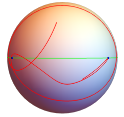
Figure 1: A free-fall periodic orbit (solid red curve) on the shape-space sphere. Notice the two open ends, one above and another below the equator.

2 Preliminaries

There are certain general features of three-body problem, as well as some features specific to the free-fall case, that need to be specified.

2.1 Three-Body Jacobi Variables

Because the return proximity function is a function of twelve variables, it is difficult to systematically vary all twelve initial conditions to find a periodic solution. Therefore we eliminate all constants of the motion, and thus reduce the number of variables of the proximity function. One way to do this is by changing the three-body Cartesian variables to relative (Jacobi) ones and to the shape sphere. We shall use the latter for classifying periodic solutions. As most of these variables remain unchanged for arbitrary masses, we discuss the general case here.

The center-of-mass (CM) two-vector ${\bf R}_{\rm CM}$ is defined for arbitrary masses as

$${\bf R}_{\rm CM}=\frac{m_{1}{\bf r}_{1}+m_{2}{\bf r}_{2}+m_{3}{\bf r}_{3}}{\sum_{i=1}^{3}m_{i}}.$$ (1)

${\bf R}_{\rm CM}$ is a constant of the motion if the total linear momentum ${\bf P}={m_{1}{\dot{\bf r}}_{1}+m_{2}{\dot{\bf r}}_{2}+m_{3}{\dot{\bf r}}_{3}}$ equals zero. The three-body dynamics is simplified by using the two relative coordinate vectors introduced by Carl Jacobi:

$${\bf\rho}=\frac{1}{\sqrt{2}}({\bf r}_{1}-{\bf r}_{2})\mbox{ and }{\bf\lambda}=\frac{1}{\sqrt{6}}({\bf r}_{1}+{\bf r}_{2}-2{\bf r}_{3}),$$ (2)

which are applicable even for unequal masses. We solve the equations of motion using Cartesian coordinates and then use ${\bf\rho}$ and ${\bf\lambda}$ to graphically represent the solutions. Thus we reduce the number of variables in the proximity function $d({\bf X}_{0},T_{0})$ from twelve to eight.

2.2 Agekyan-Anosova’s initial-condition space for the free-fall problem

As per definition of the free-fall orbit, there is at least one instance in time when all three bodies are at rest. We use that instance as our initial time $t_{0}=0$, to define the initial conditions, which only concern the three bodies coordinates, i.e., the shape and the size of the triangle subtended by the three bodies. The historically accepted convention, due to Agekyan and Anosova [4], see also Tanikawa et al. [5, 8, 9]), for these variables is distinct from the shape sphere and the hyper-radius defined in 2.3. That leads to certain complications, discussed below.

The definition of the initial-condition (i.c.) space for the free-fall 3-body problem was given by Agekyan and Anosova. They put body number 2, with mass $m_{2}$ at $A(-0.5,0)$ and body number 3 with mass $m_{3}$ at $B(0.5,0)$ both on the $x$-axis of the $(x,y)$-plane. The body number 1 with mass $m_{1}$ is put at any place P within the circular segment

$${\cal D}=\left\{(x,y):x\geq 0;y\geq 0;(x+0.5)^{2}+y^{2}\leq 1\right\}.$$ (3)

This is the Agekyan-Anosova domain ${\cal D}$, see Fig. 2.

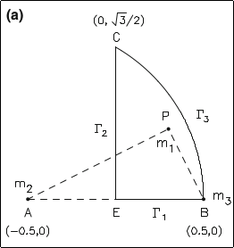
Figure 2: The initial position of three bodies in the configuration space. The initial positions of mass no. 2 and mass no. 3 are located at points $A(-0.5,0)$ and $B(0.5,0)$, respectively. The initial position of mass no. 1 is at the point $P(x,y)$ in the region ${\cal D}$.

As Tanikawa [5] noted, this is not a unique choice, as can be seen by the fact that the vertical $x$ axis in Fig. 2 describes isosceles triangles, but so does also the circular boundary of the Agekyan-Anosova domain ${\cal D}$.

There are three other similar (in the sense that they can be obtained by reflections, about the $x$, and/or the $y$ axis, from this one) domains, another four compact and four infinite domains (12 in toto). They correspond to spatial reflections and different permutations of mass labels (1,2,3) of the three bodies, see Fig. 3.

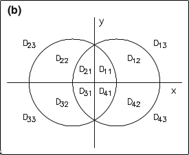
Figure 3: Tanikawa’s triangle shape space. $D_{11}$ corresponds to the D-shaped domain in Fig. 2. The other $D_{ij}$ are obtained by reflections. For example, $D_{21}$ is the mirror image of $D_{11}$ with respect to the $y$-axis; $D_{12}$ is the mirror image of $D_{11}$ with respect to their boundary circle (cf. [9]).

Permutation symmetry is perhaps most easily seen/illustrated on the shape sphere, see Fig. 4 in Sect. 2.3, where cyclic permutations correspond to rotations through $2\pi/3$ about the $z$-axis, whereas two-body permutations correspond to reflections about three Euler meridians. These meridians partition the shape sphere into six “slices”/wedges, each one having a half “north” and “south” of the equator. These 12 sectors correspond to Tanikawa’s 12 sectors in the $(x,y)$ plane, see Fig. 3.

An apparent advantage of the Agekyan-Anosova domain ${\cal D}$ over some of the other domains is that it is finite, but that may, in certain cases be an actual disadvantage, considering the fact that there are (probably) infinitely many periodic orbits located in a finite area. That means potentially high or even infinite density of periodic orbits, at least near the two-body collision points in the Agekyan-Anosova domain ${\cal D}$.

2.3 The shape space of triangles

There are three independent scalar three-body variables: $\lambda^{2}$, $\rho^{2}$, and ${\rho}\cdot{\lambda}$. The hyperradius $R=\sqrt{\rho^{2}+\lambda^{2}}$ characterizes the overall size of the orbit and removes one of the three scalar variables. We may relate the three scalar variables to the unit three-vector $\hat{\bf n}$ defined by the Cartesian components

$$\hat{\bf n}=\left(\frac{2{\rho}\cdot{\lambda}}{R^{2}},\frac{\lambda^{2}-\rho^{2}}{R^{2}},\frac{2({\rho}\times{\lambda})\cdot{e}_{z}}{R^{2}}\right).$$ (4)

The domain of these three-body variables is a sphere with unit radius, [24] as illustrated in Fig. 4. The (shape) sphere coordinates depend only on the shape of the triangle formed by the three bodies, not on $R$ or on its orientation. The equatorial circle corresponds to collinear three-body configurations (degenerate triangles). The three points shown in Fig. 4 correspond to two-body collisions, that is, singularities in the potential, see also Fig. 5.

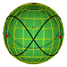
Figure 4: Figure-eight orbit (solid closed curve) on the shape-space sphere. Three two-body collision points (red), singularities of the potential, lie on the equator.

Two angles parametrizing the shape sphere together with the hyperradius $R$ define the three-dimensional configuration space of the planar three-body problem.

The Smith-Iwai permutation-adapted (hyper)spherical angles ($\alpha$, $\phi$) are defined as follows

$$\hat{\bf n}=\left(\sin\alpha\cos\phi,\sin\alpha\sin\phi,\cos\alpha\right).$$ (5)

which leads to

$$\cos\alpha = \left(\frac{2{\rho}\times{\lambda}}{R^{2}}\right),$$ (6)

$$\tan\phi = \left(\frac{n_{x}^{{}^{\prime}}}{n_{y}^{{}^{\prime}}}\right)=\left(\frac{2{\rho}\cdot{\lambda}}{{\rho}^{2}-{\lambda}^{2}}\right).\$$ (7)

We see that the sign of $\cos\alpha$ changes every time the trajectory crosses the equator, or, equivalently, whenever the triangle passes through a syzygy (collinear configuration). Permutations are directly related to rotations about $z$-axis, i.e., to changes of the meridional angle $\phi$, see below.

Unlike many “conventional” periodic orbits, the free-fall orbits do not close a loop on the shape sphere, but rather form an open section of a curve, with two open ends, see Fig. 1. Consequently, the topology of such a curve cannot be defined in the same way as for closed loops, see Sect. 2.4.

The natural domain of the permutation symmetric 3-body variables is a circle with unit radius, see Fig. 5. The points on the unit circle correspond to collinear configurations (“triangles" with zero area), or syzygies.

The permutation group on three objects $s_{3}$ consists of 6 elements, divided into 3 conjugacy classes, see textbooks, such as Stancu’s [26] §4 Permutation group $s_{n}$ and in Elliott and Dawber’s [27] §17 Permutation group $s_{n}$.

The two straight lines at angles of $\pm\frac{2\pi}{3}$, together with the vertical axis in Fig. 5 are the three (reflection) symmetry axes; these reflections correspond to the three “two-body permutations"/transpositions in the $s_{3}$ permutation group. The two cyclic permutations of the $s_{3}$ permutation group correspond to the rotations through $\pm\frac{2\pi}{3}$.

The six points where the symmetry axes cross the big circle in Fig. 5 correspond to either a) three collinear configurations (“shapes") in which one pair of particles has vanishing separation (big solid circles), i.e., “sits on top of each other", or b) three collinear configurations (“shapes") in which one particle has equal separation from the other two, i.e. “sits in the middle between the other two" (small solid circles). The center of the circle corresponds to the equilateral triangle configuration (“shape”), which turns into a point when the hyper-radius $R\to 0$.

Note how the equatorial circle is divided into six identical “pizza slices”/wedges, which number is doubled on the shape sphere, as, for each “pizza slice” in the equatorial plane there are two (equal-area) parts on the shape sphere: one “north” and one “south” of the equator, which are each other’s mirror image.

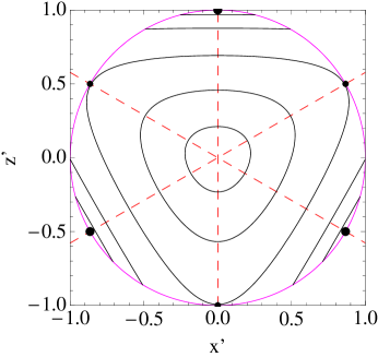
Figure 5: (Color online) Contour plot of the logarithm of the sum of Newton’s two-body potentials for any fixed value of the hyper-radius $R$ in the equatorial plane of the shape sphere. The two straight dashed red lines at angles of $\pm\frac{2\pi}{3}$, and the vertical axis are the symmetry axes, i.e., the $s_{2}$ subgroups of the $s_{3}$ permutation group. The three collinear configurations in which one pair of particles has vanishing separation (“collision points”) are denoted by big solid circles, and the three collinear (“Euler points”) configurations in which one particle has equal separations from the other two are denoted by small solid circles. As one approaches the two-body collision points (three large solid points on the big circle), the equipotential contour lines become increasingly dense, finally reaching infinite density at these points, due to the singularities/poles present.

2.4 Syzygies as symbolic sequences for free-fall periodic orbits

As stated in the Introduction, Sect. 1, Montgomery’s method [24] of associating free-group elements does not work for periodic free-fall orbits, because they do not form a closed loop on the shape sphere. Rather, we use Tanikawa and Mikkola’s method [8, 9] of associating a (finite) sequence $w(0,T)=s_{1}s_{2}s_{3}\ldots$ of three symbols $s_{i}$, say the numbers 1, 2 and 3 with each periodic orbit with period $T$. The three symbols/numbers (1,2,3)/ correspond to one of the three segments on the equator of the shape sphere wherein the orbit crosses the equator (which is guaranteed to happen by Montgomery’s theorem 2007 [28]).

Of course, that still leaves us with an ambiguity regarding permutations. Moreover, we shall only associate symbolic sequences with one half of the period $w(0,T/2)$, as the second half of a periodic orbit is represented by the (exact) inverse symbolic sequence $w(T/2,T)=w^{-1}(0,T/2)$, leaving a trivial (“unity”) sequence for (every) complete periodic orbit $w(0,T)=w(0,T/2)w(T/2,T)=1$.

Each time a triple system becomes collinear, a symbol is given according to the rule described at the top of this subsection. Therefore, an orbit, except the one which terminates at triple collision, represented by an infinite continuous curve in the phase space is replaced by a bi-infinite (corresponding to the past and future) symbol sequence. We denote the symbols by $s_{i}$ and the boundary between the past and future (zero time $t=0$ initial condition) by a period ($\bullet$), the present state being just after the period. Here we only consider the future symbol sequences. Then a (future) symbol sequence $s$ starting at the present can be written as

$$s=\bullet s_{1}s_{2}s_{3}\ldots~{}~{}~{}~{}~{}~{}~{}~{}~{}~{}~{}~{}(10)$$

Now, suppose that all the points in the initial condition plane have their own symbol sequences (10), that is, the orbits starting at points of the initial condition plane are all integrated to the future. Of course, triple collision orbits have finite symbol sequences. If we truncate the symbol sequences at the $n$-th digit, there are a finite number of possible combinations of symbols in these length-$n$ “words”. The point set of the initial condition plane whose symbol sequences contain a particular initial word of length n is called an “$n$-cylinder”. For each $n$, a finite number of $n$-cylinders divide the initial condition plane into different sections. Boundaries of the cylinders are formed with binary collision curves (BCCs) [9, 10].

We use the shape sphere, as defined in 2.3 and in Ref. [29], to define the equator and syzygies.

3 Results

3.1 The return proximity function

The return proximity function $d({\bf X}_{0},T_{0})$ in phase space is defined as the absolute minimum of the distance from the initial condition by $d({\bf X}_{0},T_{0})=\min_{t\leq T_{0}}|{\bf X}(t)-{\bf X}_{0}|$, where

$$\left|{\bf X}(t)-{\bf X}_{0}\right|=\sqrt{\sum_{i}^{3}[{\bf r}_{i}(t)-{\bf r}_{i}(0)]^{2}+\sum_{i}^{3}[{\bf p}_{i}(t)]^{2}}$$ (8)

is the distance (Euclidean norm) between two 12-vectors in phase space (the Cartesian coordinates and velocities of all three bodies without removing the center-of-mass motion). Searching for periodic solutions with a period $T$ smaller then a parameter $T_{0}$ is equivalent to finding zeros of the return proximity function. In this work, the value of $T_{0}$ is taken to be $T_{0}(x,y)=\min(7,80/|E(x,y)|^{3/2})$. The numerical algorithm that we use for finding periodic orbits is in principle those used in [22, 15]. This is the grid-search algorithm in combination with Newton’s method [30], where the computing of the coefficients of the linear system at each step of Newton’s method is done with the high order Taylor series method used with high precision floating point arithmetic [31]. The obtained better efficiency from us can be explained with the use of a finer search-grid, the use of a modification of Newton’s method with a larger domain of convergence [32], and some technical improvements. The numerical method will be given in much detail elsewhere.

3.2 Distribution of i.c.s in Agekyan-Anosova’s domain ${\cal D}$

As a result of the search in Agekyan-Anosova’s domain ${\cal D}$ with the restriction for the periods $T(x,y)<\min(7,80/|E(x,y)|^{3/2})$, we find 15,738 i.c.s corresponding to 12,409 distinct solutions. 9080 i.c.s turn out not to be in pairs (a distinct dual i.c. with the same $T^{*}$ does not exist). Simulating these 9,080 i.c.s up to $T/2$ and finding the i.c.s such that the triangle formed from the three bodies is similar to the triangle formed at $T/2$ (plus possibly a permutation of mass labels), we find 8,844 secondary i.c.s, bringing the number of i.c.s up to 24,582. This way we find together with some missed by the search i.c.s, also i.c.s for $T>7$ and $T^{*}<80$, i.e. this is a cheap way that easily compensate (to some extent) that we use the condition $T(x,y)<\min(7,80/|E(x,y)|^{3/2})$ instead of the ultimate but much more time consuming condition $T(x,y)<80/|E(x,y)|^{3/2}$. Additionally, this procedure is a way to identify the self-dual i.c.s, which means that the triangles at $t=0$ and $t=T/2$ are congruent and the time evolution takes an i.c. at $T/2$ into its mirror image (plus possibly a permutation of mass labels), and then back again. We obtain $236=9,080-8,844$ such solutions. We will discuss them in 3.4.

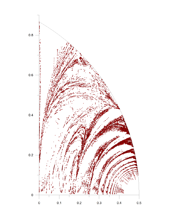
Figure 6: The 24,582 initial conditions of 12,409 free-fall orbits, including 236 self-dual ones.

All 24,582 i.c.s ordered by $T^{*}$ and given in the form of four numbers $(x,y,T,T^{*})$ with 80 correct digits can be downloaded from [33]. All symbolic sequences (“words”) discussed in 2.4 with their half-length $N/2$ and the plots in the real-space of some hundreds of the first orbits can be also found in [33].

The distribution of i.c.s can be seen in Fig. 6. It is to be noted here that the structure of the picture is very similar to the pictures for ejection times and homology map in [12] and also the picture for escape regions, binary collision curves, and triple collision points in [7]. Particularly it is seen from [7] that the distribution of i.c.s avoids the fast escape regions and is along the binary collision curves.

The plots in the real-space for the simplest asymmetric solution (with $N/2=5$), represented by two distinct i.c.s, is given in Fig.7. The initial triangle for this solution is very closed to equilateral triangle, which leads to the Lagrange’s triple collision orbit. Although one can suppose a symmetry in this solution by observing its plots, it is not the case, as seen from the zoomed versions of the plots in Fig. 8. The data $(x,y,T,T^{*})$ for this simplest solutions with 35 correct digits (approximately quadruple precision) can be seen in Table 1 (i.c.1 and i.c.2). Note that the scale-invariant periods $T^{*}$ for dual i.c.s are equal. The second simplest asymmetric solution is presented in Fig. 9 (i.c.3 and i.c.4 in Table 1).

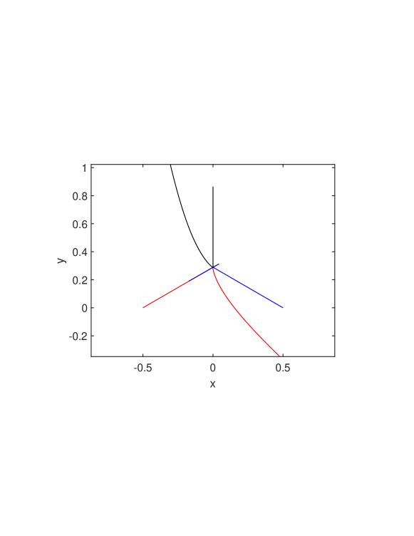
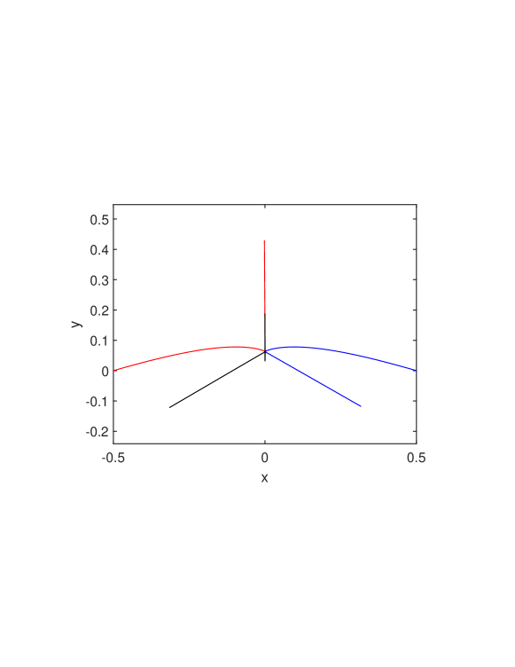
Figure 7: The simplest ($N/2=5$) asymmetric orbit represented by two i.c.s, i.c. 1 (left), i.c.2 (right)

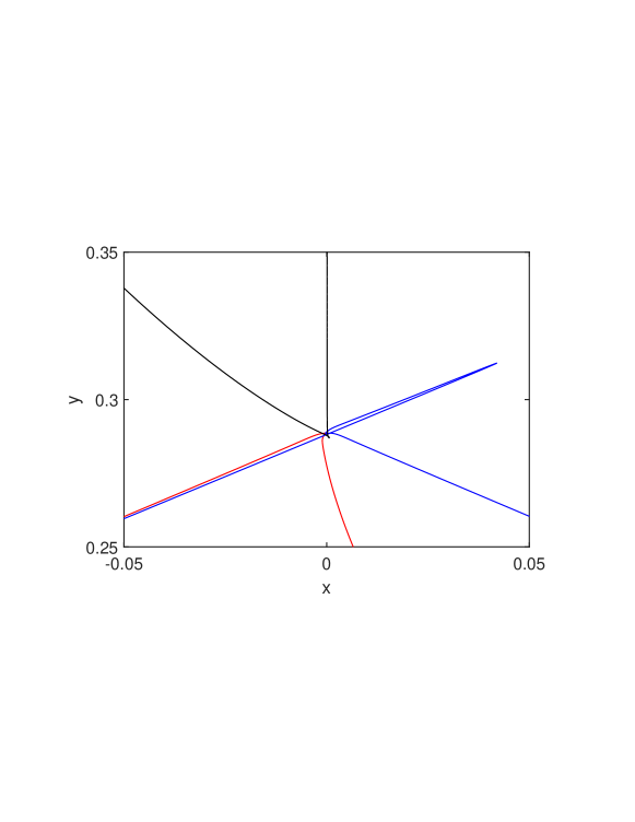
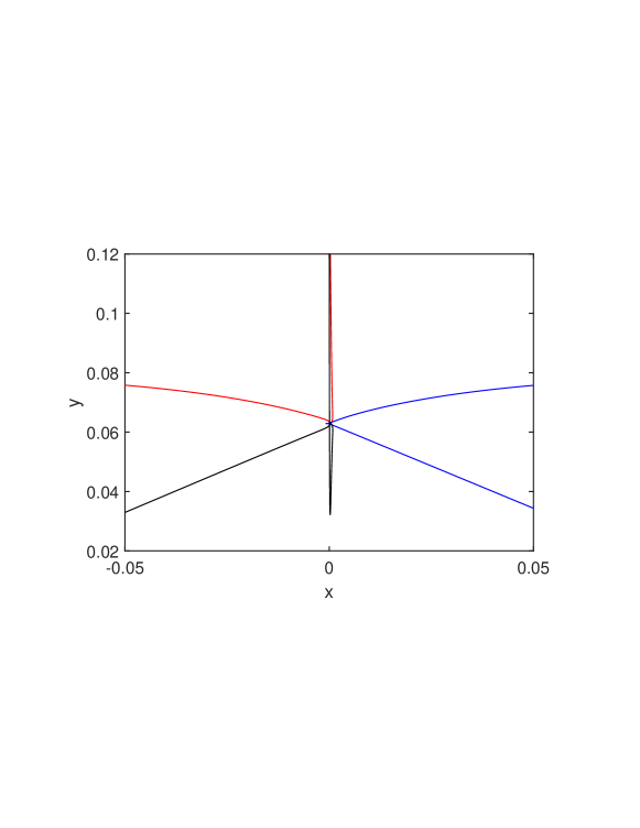
Figure 8: The simplest ($N/2=5$) asymmetric orbit (zoomed), i.c. 1 (left), i.c.2 (right)

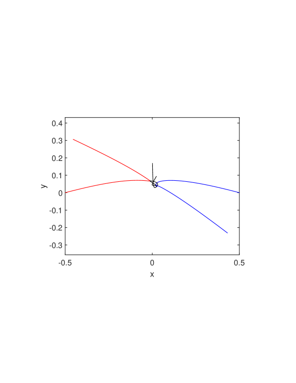
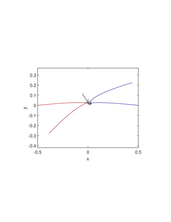
Figure 9: The second simplest ($N/2=6$) asymmetric orbit represented by two i.c.s (i.c 3, i.c. 4)

$i.c.$	$\hskip 56.9055ptx$	$\hskip 56.9055pty$	$N/2$
	$\hskip 56.9055ptT$	$\hskip 56.9055ptT^{*}$
1	0.10081002830904082427844218070523287e-3	0.86410262957299614417440390118167191e0	5
	0.27592315791656136782280882317399065e1	0.14361301848653203107026508191506541e2
2	0.20815094099721241496659892075009882e-4	0.18872009777437048186293267026882646e0	5
	0.13906231911063024951694149536454744e1	0.14361301848653203107026508191506541e2
3	0.13664936741948646596696276419442177e-2	0.16960184365485965711924464801930339e0	6
	0.14874034374340751927215339827790675e1	0.15583470416972024857327219803395329e2
4	0.61578935253763924971145321654327012e-3	0.64969497713782767052402395395661754e-1	6
	0.14078864983457596220282927174180473e1	0.15583470416972024857327219803395329e2

Table 1: Data for the first 2 simplest asymmetric solutions (4 i.c.s) with 35 correct digits

3.3 The role of binary collision curves in the Agekyan-Anosova’s domain ${\cal D}$

We insist on our orbits being collisionless, and this condition implies certain “selection rules”. Tanikawa et al. have long studied binary collision curves (BCCs) for the Newtonian free-fall 3-body problem, mostly with regard to 3-body collisions and not with regard to periodic orbits. But, their results are equally valid and applicable to periodic orbits. The big picture is that the BCCs partition the Agekyan-Anosova domain into smaller compact subdomains, which form a pattern suspiciously similar to the pattern appearing in the pictures of ejection times and of the homology map in [12].

After computing the symbolic sequences of all found i.c.s, we partition (separate) them into different sets depending on the different starting 3 or 4 symbols. This way we want to match (to agree) the results for the initial symbols of found i.c.s with Tanikawa’s division of ${\cal D}$ by $3$-cylinders and $4$-cylinders [9, 10].

In the case of considering the first three symbols we obtain three sets of i.c.s: starting with “132”, “131”, “113”. We color them in different colors - green, red, black, respectively. The binary collision curve (BCC) constituted the boundary of the 3-cylinders “132” and “131” from [9, 10] exactly separates the points with green and red color, meaning agreement (see Figure 10 (left)). There is a small number of red and black points (“131”, “113”-points) very close to the $y$-axis that make an exception (they lie in the “132” - side of the BCC). This suggest that there is a structure of small scale close to the $y$-axis with $|x|<0.01$. Computing the BCCs in this region has not yet been done, as mentioned in [10], it will be considered elsewhere.

The case of starting 4 symbols is considered analogously. Now we have 5 sets of points: starting with “1323”, “1321”, “1312”, “1313”, “1132”. We color them in blue, green, red, cyan, black, respectively. The four binary collision curves (BCCs) constituted the boundary of the 4-cylinders from [9, 10] exactly separates the points with different colors (see Figure 10 (right)), with the small exception mentioned above.

In the 4-cylinder 1132 close to the y-axis with $|x|<0.01$ (these are almost isosceles triangles close to the Euler point) there are several examples of periodic orbits (13 i.c.s) that appear as the long awaited "stutter" orbits of [34]; we hope to return to this subject elsewhere.

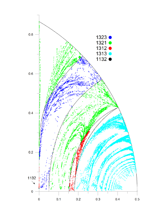
Figure 10: Partitioning of i.c.s in ${\cal D}$ by $3$-cylinders(left) and $4$-cylinders(right). Boundaries of the cylinders are formed with binary collision curves (BCCs) (the black curves inside ${\cal D}$)

3.4 Self-dual (symmetric) orbits

The self-dual orbits are those for which the triangles formed by the three bodies at $t=0$ and $t=T/2$ are congruent, i.e. dual i.c.s coincide. We obtain 236 self-dual solution ($\sim 2\%$ from all 12,409 solutions), which contrast to the large number of $\sim 43\%$ (12 from 28) of Li an Liao. This ambiguity can be explained by the assumption that these solutions are generally easier to be caught numerically. Also the percent of self-dual solutions among all solutions may depend on the considered value of $T^{*}$.

The beautiful spatiotemporal symmetry of the self-dual solutions was for the first time discussed in [23]. Here we present the 8 simplest ones, found by us. Their initial conditions with 35 correct digits is given in Table 2. The corresponding plots in real-space are given in Figures 11, 12, 13, 14. For all solutions, the map that gives on what vertex (mass label) each mass label in the initial triangle maps at $T/2$, is computed. For this map two possibilities are observed - or is an identity, or two indices are permuted. All self-dual solutions have the property that if we read the first half of the symbolic sequence from back to front and apply the map of vertices, the same sequence is obtained. The symbolic sequences in their first half, their half-length $N/2$, the maps of the mass-labels and the permutations of mass-labels are given in Table 3.

According to the type of symmetry, the solutions are divided into two types. The first type of symmetry is a reflection with respect to a line. In this case the initial triangle have to be flipped in order to match the second one in the plane. These are solutions with i.c.s 4,5,6,7. In the case of this type of symmetry $N/2$ can be either even or odd. In the case of odd N/2 the map of the mass label is identity, and at T/4 the bodies lie on the axis of symmetry, in particular they are in syzygy (see i.c.s 4, 5, 6 for example). In the case of even N/2 two of the labels are always in permutation and in T/4 the body, which is not in permutation, lies on the axis of symmetry, and the other two do not lie, but are symmetrically located with respect to the axis (see i.c. 7 for example).

The second type of symmetry is a central symmetry with respect to a point. In this case the the triangles at t=0 and t=T/2 are obtained from each other with a rotation of 180 degrees. In this case $N/2$ is always odd and we always have a permutation of the labels of two of the bodies. At T/4, the bodies are in a syzygy, more precisely in “Euler configuration”. The body in the middle is at the center of the symmetry and is the one that is not in permutation.

The observed properties of self-dual solutions are valid not only for here presented 8 of them, but for all. The plots of all self-dual solutions and the maps of mass-labels can be downloaded from [33].

$i.c.$	$\hskip 56.9055ptx$	$\hskip 56.9055pty$	$N/2$
	$\hskip 56.9055ptT$	$\hskip 56.9055ptT^{*}$
1	0.26853656879186094505164950733431843e-2	0.42051392341346323788698432377477461e0	5
	0.17803915330283836111234811629291376e1	0.14571737413553345363987962673353442e2
2	0.25694268581619406691269277542214527e0	0.27837466215631876401730693017725991e0	9
	0.21573615905021502937878732480336593e1	0.23729532401436922562439610275290658e2
3	0.25332955503585550078385245318739793e0	0.27395770000593360665609561689957488e0	9
	0.21486559741398094220093978785190743e1	0.23736057405684383328815469131959677e2
4	0.19608584373815407759186511872283212e0	0.12660087703751815111408497535170496e0	9
	0.19217736055334080320628254532331719e1	0.24456532037265669456189334514166059e2
5	0.21274288450316301296609635701735616e0	0.17736655380296837596730716436202892e0	9
	0.19915034464414970230624542166422446e1	0.24461630150799015077336406520614186e2
6	0.18896979078998075365597202763735798e0	0.10009595939299847925976966044966423e0	9
	0.18986434607202684769707963605898842e1	0.24469227124446530028878538869391828e2
7	0.15490107430442084270412195964824131e0	0.64608703728749114087928822042577474e0	10
	0.47578526770531448171326235767256789e1	0.30518409889739183020522928827494681e2
8	0.32792607131573432231865988797878982e0	0.21215354249540216269360745135067314e0	13
	0.22662686790481644958133858818197705e1	0.31908616428117479764156481776483866e2

Table 2: Data for the first 8 simplest self-dual (symmetric) solutions with 35 correct digits

$i.c.$	$symbolic\hskip 5.69046ptsequence\hskip 5.69046ptat\hskip 5.69046ptT/2$	$maps\hskip 5.69046ptof\hskip 5.69046ptthe\hskip 5.69046ptlabels$	$permutations$	$N/2$
1	13213	1 $\rightarrow$ 3, 2 $\rightarrow$ 2, 3 $\rightarrow$ 1	(13)	5
2	131321313	1 $\rightarrow$ 3, 2 $\rightarrow$ 2, 3 $\rightarrow$ 1	(13)	9
3	131231232	1 $\rightarrow$ 2, 2 $\rightarrow$ 1, 3 $\rightarrow$ 3	(12)	9
4	131323131	1 $\rightarrow$ 1, 2 $\rightarrow$ 2, 3 $\rightarrow$ 3	e	9
5	131323131	1 $\rightarrow$ 1, 2 $\rightarrow$ 2, 3 $\rightarrow$ 3	e	9
6	131232131	1 $\rightarrow$ 1, 2 $\rightarrow$ 2, 3 $\rightarrow$ 3	e	9
7	1321321321	1 $\rightarrow$ 1, 2 $\rightarrow$ 3, 3 $\rightarrow$ 2	(23)	10
8	1313132131313	1 $\rightarrow$ 3, 2 $\rightarrow$ 2, 3 $\rightarrow$ 1	(13)	13

Table 3: The symbolic sequence, the maps of the mass-labels, the corresponding permutations and the half-length of the sequence for the first 8 simplest self-dual (symmetric) solutions

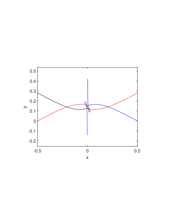
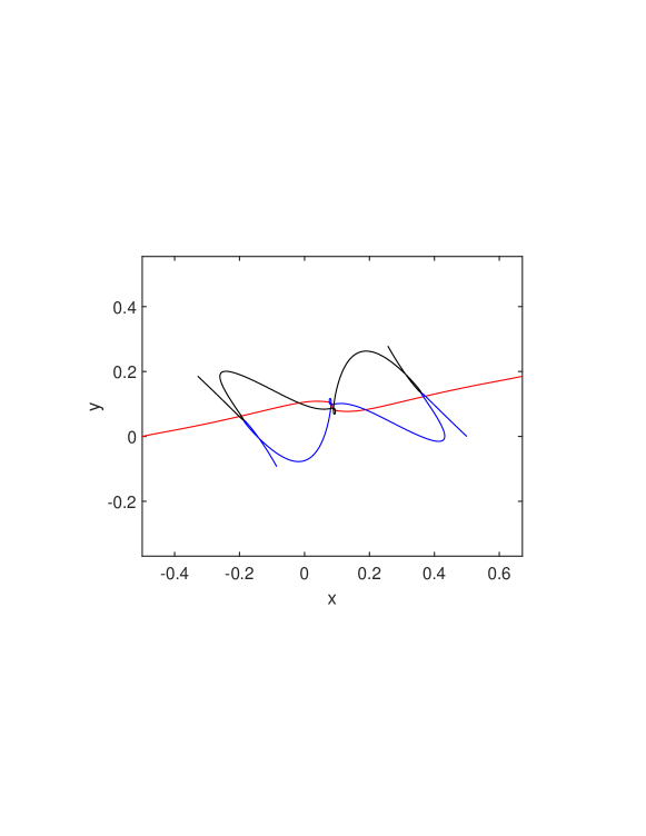
Figure 11: The simplest free-fall symmetric orbits (i.c.s 1,2, $N/2=5,9$)

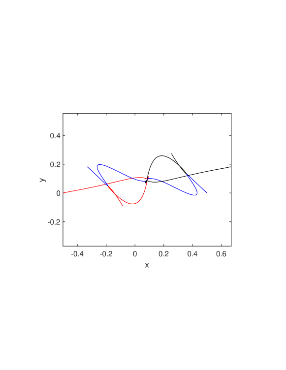
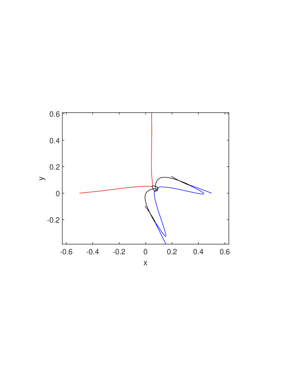
Figure 12: The simplest free-fall symmetric orbits (i.c.s 3,4, $N/2=9,9$)

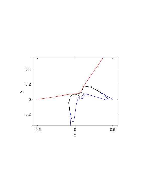
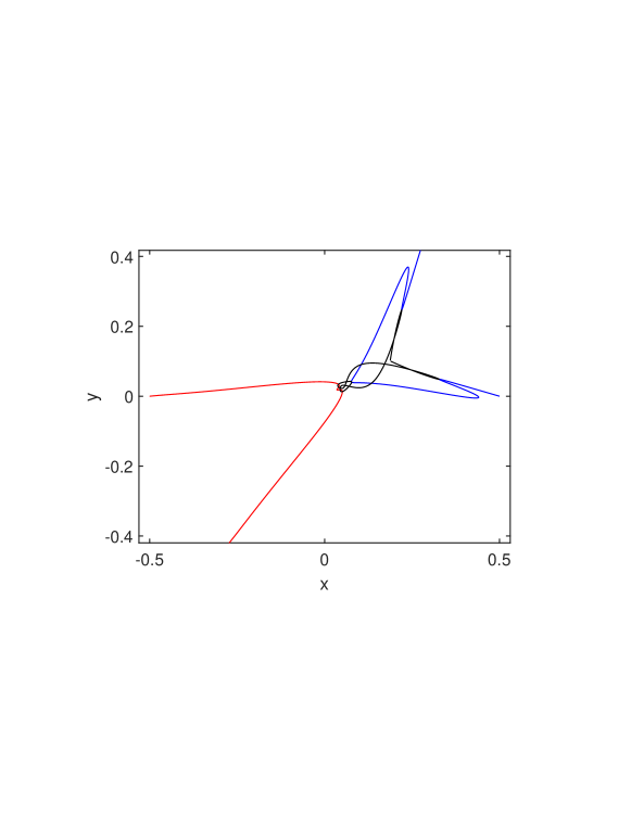
Figure 13: The simplest free-fall symmetric orbits (i.c.s 5,6, $N/2=9,9$)

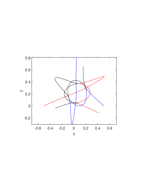
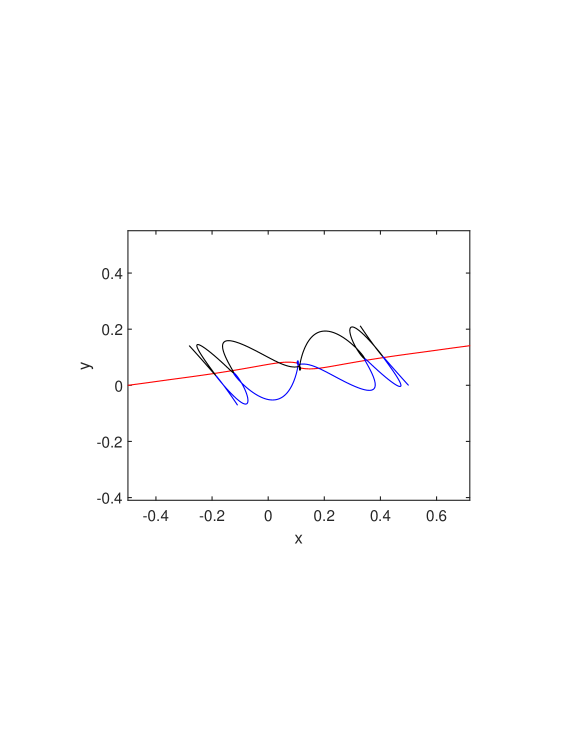
Figure 14: The simplest free-fall symmetric orbits (i.c.s 7,8, $N/2=10,13$)

3.5 Scale invariant period as function of symbolic sequence length

The scale-invariant periods turn out to be bounded from above and from below by linear functions of symbolic sequence (“word”) length, see Fig. 15. This linear dependence is in rough agreement with the linear dependence of closed-loop orbits first observed in [19] and later discussed in [20],[21] with the distinction of a larger/wider spread of the data from a straight line. That spread can be understood in terms of the argument based on the analyticity/holomorphy of the action integral, as exposed in [20],[21], however, with the following caveat: The curves on the shape sphere corresponding to free-fall orbits are not closed, but open, with two ends/terminals. A great circle can (always) be drawn through the two open ends, thus allowing two different closures of the curve, which, in turn, provide two bounds on the period.

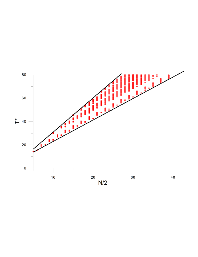
Figure 15: $T^{*}=T|E|^{3/2}$ vs. $N/2$ for all collisionless free-fall orbits.

4 Concluding remarks and Outlook

Now we summarize, conclude, and suggest future research.

1) The database of i.c.s for periodic collisionless equal-mass free-fall orbits is significantly expanded from 30 to 25,582 and up to 80 significant digits.

2) The distribution of i.c.s in the Agekyan-Anosova’s ${\cal D}$ domain shows a similar structure with many previously investigated properties of the problem in ${\cal D}$. Indeed there is a close correspondence with BCCs which correspondence ought to be explored further.

3) We found 236 self-dual (symmetric) solutions, which are only $\sim 2\%$ from all solutions. These 236 symmetric orbits ought to be of particular interest to mathematicians [23].

4) We found several examples of periodic orbits in the 4-cylinder 1132 (almost isosceles triangles close to the Euler point) that look like the long awaited "stutter" orbits of [34]. More about them elsewhere.

5) We obtain an agreement of computed symbolic sequences of the found i.c.s. with Tanikawa’s division of Agekyan-Anosova’s domain ${\cal D}$ by $3$-cylinders and $4$-cylinders. This correspondence ought to be extended to higher n-cylinders

6) The results suggest that the scale-invariant periods are bounded from above and from below by linear functions of symbolic sequence length, which is in agreement with previous results regarding closed-loop periodic orbits. This can/should be studied in greater detail.

7) Stability of orbits is of particular interest, both because of the Birkhoff-Lewis theorem and of itself.

Acknowledgments The authors I.H. and R.H. acknowledged the access to the Nestum cluster @ HPC Laboratory, Research and Development and Innovation Consortium, Sofia Tech Park. V.D. thanks Mr. Bogdan Raonić for his help in the early stages of this work. The work of V.D. was funded by the Serbian Ministry of Education Science and Technological Development, grant number 451-03-68/2020-14/200024.

References

- [1] V. Szebehely, and C. F. Peters, “Complete Solution of a General Problem of Three-Bodies”, Astron. J. 72, 876-883 (1967).
- [2] Standish, E. M.: 1970, in G. E. O. Giacaglia (ed.), Periodic Orbits, Stability and Resonances, D. Reidel Publ. Co., Dordrecht, Holland, p. 375-381.
- [3] M. Hénon, Celest. Mech. 10, 375-388 (1974).
- [4] T.A. Agekyan and Z.P. Anosova, “A study of the dynamics of triple systems by means of statistical sampling. Sov. Astron. Zhur. 44, 1261 (1967) (in Russian); Soviet Phys. Astron. 11, 1006 (1968).
- [5] K. Tanikawa, H. Umehara and H. Abe, “A search for collision orbits in the free-fall three-body problem I. Numerical procedure”. Cel. Mech. 62, 335-362 (1995).
- [6] K. Tanikawa, H. Umehara, “Oscillatory orbits in the planar three-body problem with equal masses”, Celestial Mechanics and Dynamical Astronomy 70: 167-180, (1999).
- [7] H. Umehara, and K. Tanikawa. “Binary and triple collisions causing instability in the free-fall three-body problem.” Celestial Mechanics and Dynamical Astronomy 76.3: 187-214, (2000)
- [8] K. Tanikawa and S. Mikkola, “A trial symbolic dynamics of the planar three-body problem”, Proc. “Resonances, Stabilization, and Stable Chaos in Hierarchical Triple Systems”, ed. V. V. Orlov & A. V. Rubinov, St Petersburg State University Press, St Petersburg, (2008), pp. 26. (arXiv:0802.2465)
- [9] K. Tanikawa, and S. Mikkola, “Symbol sequences and orbits of the free-fall three-body problem”, Publications of the Astronomical Society of Japan (2015), Vol. 67, No. 6, 115 (2015).
- [10] Kiyotaka Tanikawa, Masaya M. Saito and Seppo Mikkola “A search for triple collision orbits inside the domain of the free-fall three-body problem”, Celestial Mechanics and Dynamical Astronomy (2019) 131:24
- [11] Xiaoming Li, Xiaochen Li, Linghui He and Shijun Liao, “Triple collision orbits in the free-fall three-body system without binary collisions”, Celestial Mechanics and Dynamical Astronomy 133: 46 (2021).
- [12] H. J. Lehto, S. Kotiranta, M. J. Valtonen, P. Heinämäki, S. Mikkola and A. D. Chernin, “Mapping the three-body system – decay time and reversibility” Mon. Not. R. Astron. Soc. 388, 965–970 (2008)
- [13] P. P. Iasko and V. V. Orlov, Astronomy Reports, Vol. 58, No. 11, pp. 869-879 (2014).
- [14] P. P. Iasko and V. V. Orlov, “Search for Periodic Orbits in in Agekyan and Anosova’s Region D for the General Three-Body Problem”, Astronomy Reports, Vol. 59, No. 5, pp. 404-413 (2015).
- [15] Xiaoming Li and Shijun Liao, “Collisionless periodic orbits in the free-fall three-body problem”, New Astronomy 70, 22-26 (2019); arXiv:1805.07980v1 (nlin).
- [16] Milovan Šuvakov, and V. Dmitrašinović, Phys. Rev. Lett. 110, 114301 (2013).
- [17] Milovan Šuvakov, Celest. Mech. Dyn. Astron. 119, 369-377 (2014).
- [18] http://suki.ipb.ac.rs/3body/index.php
- [19] V. Dmitrašinović and M. Šuvakov, “Topological Dependence of Kepler’s Third Law for Collisionless Periodic Three-Body Orbits with Vanishing Angular Momentum and Equal Masses”, Phys. Lett. A 379, 1939-1945 (2015).
- [20] V. Dmitrašinović, Ana Hudomal, Mitsuru Shibayama, Ayumu Sugita, “Linear Stability of Periodic Three-Body Orbits with Zero Angular Momentum and Topological Dependence of Kepler’s Third Law: A Numerical Test”, J. Phys. A: Math. Theor. 51, 315101 (2018), arXiv:1705.03728 [physics].
- [21] V. Dmitrašinović,, Luka V. Petrović and Milovan Šuvakov, “Periodic three-body orbits with vanishing angular momentum in the pairwise “strong” potential”, Jour. Phys. A 50, 435102 (2017).
- [22] Xiaoming Li and Shijun Liao, “More than six hundred new families of Newtonian periodic planar collisionless three-body orbits”, Sci. China-Phys. Mech. Astro. Vol. 60 No. 12: 129511 (2017).
- [23] Montgomery, Richard. "Dropping Bodies." The Mathematical Intelligencer (2023): 1-7.
- [24] R. Montgomery, Nonlinearity 11, 363 - 376 (1998).
- [25] http://hpc-lab.sofiatech.bg/
- [26] Fl. Stancu, “Group Theory in Subnuclear Physics”, Clarendon, Oxford, UK (1996).
- [27] JP Elliott, PG Dawber, “Symmetry in physics vol. 2, Principles and simple applications ”, Oxford University Press (1984).
- [28] Montgomery, Richard. “The zero angular momentum, three-body problem: All but one solution has syzygies” Ergodic Theory and Dynamical Systems 27.6 (2007): 1933-1946.
- [29] M. Šuvakov, and V. Dmitrašinović, “A guide to hunting periodic three-body orbits”, Am. J. Phys. 82, 609–619 (2014).
- [30] Abad, Alberto, Roberto Barrio, and Angeles Dena. “Computing periodic orbits with arbitrary precision” Physical review E 84.1 (2011): 016701.
- [31] Barrio, Roberto, et al. “Breaking the limits: the Taylor series method” Applied mathematics and computation 217.20 (2011): 7940-7954.
- [32] I.Hristov, R.Hristova, I. Puzynin, et al. “Newton’s method for computing periodic orbits of the planar three-body problem.” arXiv preprint arXiv:2111.10839 (2021).
- [33] http://db2.fmi.uni-sofia.bg/3bodyfree/
- [34] Richard Moeckel, Richard Montgomery & Andrea Venturelli, “From Brake to Syzygy”, Arch. Rational Mech. Anal. 204 (2012) 1009-1060. DOI: 10.1007/s00205-012-0502-y