Utilizing smartphone sensors for accurate solar irradiance measurement and educational purposes

Abstract

The global transition towards cleaner and more sustainable energy production is a major challenge. We present an innovative solution by utilizing smartphone light sensors to measure direct normal solar irradiance, the primary component of ground-level solar radiation. We provide comprehensive guidelines for calibrating the sensor using two methods: a professional reference measurement and clear-sky satellite estimates. The latter method is particularly advantageous in resource-constrained environments. Once calibrated, the smartphone becomes a valuable tool for measuring the solar resource. After calibrating the device, we propose an instructional laboratory focusing on the physics of solar radiation and its interaction with the Earth’s atmosphere, exploring solar variations across locations, cloud conditions, and time scales. By integrating irradiance values measured throughout a day the daily irradiation can be estimated. This approach enhances students’ understanding of solar radiation attenuation and its relationship with atmospheric interactions. This method offers a practical and educational solution for promoting renewable energy knowledge and addressing the challenges of the energy transition.

1 Introduction

The rise of renewable energy sources, particularly solar and wind power, is an unstoppable force [1, 2]. This transformative shift in energy production and consumption necessitates a workforce equipped with specialized knowledge and skills. However, the incorporation of renewable energy topics in science and engineering curricula, especially in physics courses, has often been marginalized. Specifically, the study of solar radiation is predominantly approached from a theoretical standpoint, potentially due to the technical complexities and high costs associated with measurement instruments. As a result, experiments involving the measurement of solar irradiance and the determination of its uncertainty are typically reserved for advanced programs or specialized laboratories.

The importance of the contents associated with solar energy transcends its specific aspects. In fact, this subject matter provides a platform to develop various cross-cutting competencies, including measurement techniques and environmental stewardship. In summary, the dissemination of instructional laboratories focusing on clean and environmentally sustainable methods of energy production serves the dual purpose of encouraging responsible citizen engagement in public policy discussions and training professionals who can contribute to the growth of the sector.

The proposal of this article makes it possible to break down the cost barrier making it possible to incorporate in undergraduate experimental physics courses. The cost barrier is eliminated through the use of smartphones as a measurement instrument, which have also shown innovative contributions to the teaching of Physics for different thematic areas [3, 4, 5]. We show here how to use a smartphone’s light sensor [6] to measure broadband direct solar irradiance at normal incidence (DNI), the main component of solar radiation at ground level. Direct irradiance is the portion of the incident radiation that arrives directly from the solar disk without being absorbed or scattered in the Earth’s atmosphere. This component is essential to evaluate the performance of concentrating solar applications and to estimate the solar irradiance available on an inclined plane, necessary for solar photovoltaic and low-temperature solar thermal applications in which it is usual practice to tilt the solar collection surfaces. Here, we describe two procedures for calibrating the sensor, one based on a professional reference measurement and the other using publicly-available satellite estimates of ground level clear-sky irradiance. In both cases we pay special attention to non-trivial implementation details. We compare the calibration procedures and show that both are feasible. By bridging this gap about calibration, we enable the measurements and instructional laboratory to be done with only the smartphone and manual positioning, if required. The instructional laboratory proposed here has a focus on solar resource fundamentals, which are required to understand any form of solar energy application.

This article is organized as follows. Next section introduces the basic aspects of solar radiation modeling, the various magnitudes and usual geometric calculations in the area of solar energy and lighting. Section 3 shows the experimental setup carried out in this work for the professional calibration of the illuminance sensor of a smartphone for the measurement of DNI. This section also introduces the solar satellite estimates, which are used here as an alternative reference data set for smartphone calibration. These data are publicly available for download on dedicated websites with global coverage, so their use does not represent a limitation. Section 4 describes the calibration process and its uncertainty evaluation against both sets of data. Once the sensors are calibrated it is possible to propose different activities. Specifically in Section 5 we propose several activities that can conform an instructional laboratory in this area. Finally, Section 6 summarizes the conclusions.

2 Theoretical framework: solar radiation

The solar irradiance, $G$, is the incident power per unit normal surface whose beam comes from the Sun. The solar irradiance at the top of the atmosphere, $G_{o}$, varies because of two factors: a variation of about $\pm 3$% due to the elliptical character of the Earth’s orbit around the Sun, and also, it present small variations due to oscillations in the solar activity, typically below $0.3$% [7]. The averaged solar irradiance at the top of the atmosphere on a surface normal to the Earth-Sun direction and when the Earth is at a distance equal to the mean Earth-Sun distance (1 Astronomical Unit or AU) is known as the solar constant [8], $G_{sc}=1361$ Wm^-2. In this way, the seasonal variation of $G_{o}$ is obtained by multiplying the solar constant by the orbital factor, $F_{n}=1/r^{-2}$, accounting for the variation of the Earth-Sun distance and it can be approximated with an uncertainty of 0.25% by

$$F_{n}=1+0.033\times\cos\left(\frac{2\pi n}{365}\right),$$ (1)

where $n$ is the ordinal day number (going from 1, Jan. 1st. to 365 Dec. 31) [9, 10]. The extraterrestrial irradiance at normal incidence is obtained then as $G_{o}=G_{sc}\times F_{n}$.

Once solar irradiance penetrates the Earth’s atmosphere, it interacts with various atmospheric components such as air, aerosols, water vapor, and cloudiness. This interaction leads to scattering in multiple directions, with some of the irradiance being absorbed by these components, while the remaining portion is reflected back into space. A certain percentage of the irradiance originating from the top of the atmosphere eventually reaches the Earth’s surface. It does so through two distinct paths: (i) directly from the solar disk, without undergoing scattering or absorption by atmospheric components and (ii) from the rest of the sky, following a series of complex processes involving multiple scattering. The combination of these two components on a horizontal plane is known as the global horizontal irradiance (GHI), denoted as $G_{h}$, which represents the solar energy magnitude most commonly measured on the Earth’s surface. Several methods can be employed to measure this quantity, including the use of photodiodes, calibrated photovoltaic cells, or thermopile pyranometers. Among these options, the last offers the highest precision.

Direct normal irradiance, denoted as $G_{bn}$, is less frequently measured since its continuous measurement requires fine solar tracking mechanisms that ensure the measuring equipment to be aligned at all times pointing to the solar disk. The measuring instrument, the pyroheliometer, is equipped with a collimating tube that filters any irradiance that does not come from its normal direction, with a convention aperture of 5 sr of solid angle, corresponding to a typical solar disk. The size of the solar disk observed from Earth depends on atmospheric conditions. In the presence of high humidity, for example, the perceived solar disk enlarges due to a larger size of the circumsolar region. The solid angle of 5 sr associated with the solar disk is, in effect, a convention value. The standard that classifies solar radiation measurement instruments is the ISO 9060:2018 which establishes categories according to the quality of the equipment (offset, angular error, response time, among others) and the corresponding uncertainty. After measuring the DNI, the atmospheric transmittance can be estimated as $T_{b}=G_{bn}/G_{o}$, a quantity that allows quantifying the attenuation of the irradiance in the atmosphere, in particular, in the presence of cloudiness.

In the upcoming section our focus is on presenting a straightforward clear-sky model that relies on the Lambert-Beer-Bouger law. To establish this model, we must first define several geometric quantities. One quantity is the solar zenith angle, denoted as $\theta_{z}$, which represents the angle between the direction of the Sun and the local vertical (referred to as the local zenith) as shown in Fig. 1a. The cosine of this angle appears recurrently in expressions related to solar radiation, especially for magnitudes projected onto the horizontal plane, and its calculation is carried out according to [10]

$$\cos\theta_{z}=\cos\phi\cos\delta\cos\omega+\sin\phi\sin\delta,$$ (2)

where $\phi$ is the latitude, $\delta$ is the solar declination angle and $\omega$ is the hour angle shown in Fig. 1b. Latitude is the angle between the Earth’s equator (parallel 0°) and the site of interest (indicated by $\mathcal{O}$ in the figure), along the observer’s meridian. By convention, latitudes are positive north of the equator and negative south of the equator. Solar declination is the angle formed by the Earth-Sun line with the Earth’s equatorial plane, and can be calculated in radians with good precision through the expression:

$$\delta=0.4095\times\sin\left(2\pi~{}\frac{(n+284)}{365}\right).$$ (3)

Finally, the hour angle is the angle on the equatorial plane between the observer’s meridian and the solar meridian. This angle varies with the apparent position of the Sun respect to the Earth and it is calculated from the time label associated with each measurement. Figure 1b also depicts a fourth relevant angle, $\psi$, the longitude of the observer measured from the Greenwich meridian ($\psi=0$°).

The hour angle is related to the solar time of the site, $t_{s}$, according to

$$\omega=\frac{\pi~{}(t_{s}-12)}{12}.$$ (4)

Indeed, this angle is $w=0$ at solar noon ($t_{s}=12$ hours), i.e. when the solar meridian coincides with the observer’s meridian, and grows at a rate of $\pi/12$ radians per hour, the speed of rotation of the Earth. To complete the calculation, it remains to link the solar local time with the local standard time, $t_{u}$, expressed according to a given UTC time zone associated to a central meridian, $\psi_{u}$. For example, the time in UTC-3 is associated with a meridian of $\psi_{u}=-45$°. The relationship between both hours includes the so-called equation of time, $E$, and is defined by

$$t_{s}=t_{u}+\frac{E+4~{}(\psi-\psi_{u})}{60},$$ (5)

where $t_{u}$ is the local standard time expressed in hours and fractions, $\psi$ and $\psi_{u}$ are the signed longitude in decimal degrees (negative for West longitudes and positive for East longitudes) of the site and the reference UTC, respectively, and $E$ is expressed in minutes. Based on Spencer’s developments[11], $E$ can be calculated as a Fourier expansion in terms of the variable $\Gamma=2\pi(n-1)/365$ as

$$E=229.2(7.5\times 10^{-5}+1.868\times 10^{-3}\cos\Gamma-3.2077\times 10^{-2}\sin\Gamma-1.4615$$

$$\times 10^{-2}\cos 2\Gamma-4.089\times 10^{-2}\sin 2\Gamma).$$ (6)

(a) Cosine of the solar zenith angle.

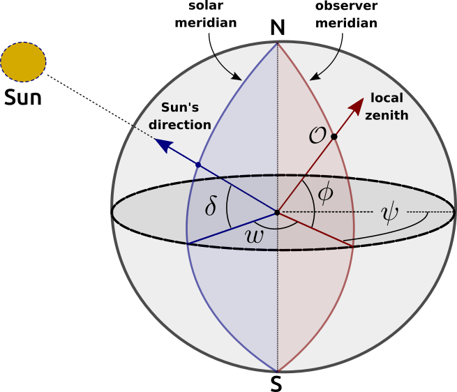
(b) $\delta$, $\phi$, $\psi$ and $w$ angles.

Figure 1: Scheme of the different angles related to the Sun’s apparent movement.

2.1 Air mass

The mass of air or relative optical mass, $m_{i}$, is a dimensionless quantity that is defined as the quotient between the amount of mass of a certain component $i$-th of the atmosphere that a beam of radiation covers in its trajectory and the one that it would cover in a vertical path, that is, in the direction of the zenith. If a non-anisotropic flat atmosphere is assumed for its calculation, the following simplified and purely geometric expression is obtained [9, 10]:

$$m_{i}=m=\frac{1}{\cos\theta_{z}}.$$ (7)

The uncertainty associated with this expression due to neglecting the terrestrial curvature and the refraction phenomena grows as the zenith angle is larger. However, the expression presents an uncertainty of about $0.25$% for $\theta_{z}=60$° [9], and it is adequate for zenith angles between 0° and 70°. There were proposed more precise expressions that can be used for large zenith angles, around 80-90°, such as that of Kasten and Young [12]. Here, as we do not consider measurements very early in the morning or very late at sunset the previous expression, Eq. 7, results appropriate.

2.2 Lambert-Beer-Bouger law

The Lambert-Beer-Bourger law describes the attenuation of a direct beam of radiation when passing through a medium. Its application to the direct normal irradiance in the atmosphere results in an exponential and spectrally selective attenuation

$$G_{b,\lambda}=G_{o,\lambda}e^{-m\tau_{\lambda}},$$ (8)

where $G_{b,\lambda}$ is the direct spectral irradiance, $G_{o,\lambda}$ is the spectral extraterrestrial irradiance corrected by the orbital factor, $\tau_{\lambda}$ is the optical depth of the atmosphere and $m$ is the air mass. This equation can be derived from the differential version of the Lambert-Beer-Bouger modeling the atmosphere by a set of layers $i$, so as the transmissivity can be expressed as $T_{i,\lambda}=\exp(-\tau_{i,\lambda}~{}m_{i})$. The total transmissivity results from the product of the layers, and therefore $\tau_{\lambda}$ includes the effect of all different components. This is a regular assumption when modeling the interaction between the Sun’s radiation and the atmosphere [13, 14].

Clear-sky models adopt the Lambert-Beer-Bouger law to describe the direct normal irradiance under ideal atmospheric conditions. In these conditions, the attenuating components encompass various factors such as air molecules (O₂, N₂, Ar), which are responsible for Rayleigh scattering, as well as water vapor, aerosols, ozone, and other minor gases. Ozone, although crucial for life on Earth due to its role in attenuating ultraviolet radiation, has a relatively minor contribution across the entire solar spectrum. A Rayleigh atmosphere refers to a pristine and dry atmospheric state where only the attenuation mechanism of molecular scattering is at play, leading to a clean and transparent atmosphere.

Numerous clear-sky models have been developed based on these concepts [15]. Among them, the ESRA (European Solar Radiation Atlas) model [16] strikes a favorable balance between simplicity and precision, making it suitable for implementation within the framework of an university experimental practice. This model operates using the concept of global optical depth, denoted as $\tau$, which encompasses the entire solar spectrum. By incorporating the global optical depth of Rayleigh extinction, denoted as $\tau_{R}$, we can express $\tau=\tau_{R}~{}T_{L}$, where $T_{L}$ represents Linke’s turbidity which quantifies the number of clean and dry atmospheres that would need to be stacked to achieve the same level of attenuation observed in the real atmosphere. Consequently, by adjusting a single parameter, $T_{L}$, based on ground measurements it becomes feasible to construct a straightforward model for estimating DNI under clear-sky conditions as $G_{bn}=G_{o}e^{-\tau_{R}mT_{L}}$. There are several ways to approximate the Rayleigh optical depth [17, 18, 12, 19, 20]. Here we use the formulation of Kasten [20], used in the ESRA model:

$$\frac{1}{\tau_{R}}=\left\{\begin{array}[]{ll}6.62960+1.75130m-0.12020m^{2}+0.00650m^{3}-0.00013m^{4}&m\leq 20\\ 10.6+0.718m&m>20.\end{array}\right.$$ (9)

2.3 Illuminance

Photometry is the area of knowledge that is responsible for measuring the light perceived by the human eye. This quantity depends on the sensitivity of the human eye to different wavelengths in the visible region of the electromagnetic spectrum. Each wavelength has its relative weight in the response of the human eye depending on the lighting conditions (good or poor) in which the observer is. In typical lighting conditions, corresponding to a real situation at Sun, it is possible to relate the illuminance, $E_{v}$, measured in lumens per unit area, lm/m² or lx, with the spectral irradiance $G_{\lambda}$ according to

$$E_{v}=K_{m}\times\int_{380}^{780}G_{\lambda}~{}V_{\lambda}~{}\mathrm{d}\lambda,$$ (10)

where $V_{\lambda}$ is the spectral response of the human eye and $K_{m}=683~{}\mathrm{lm/W}$ is the maximum luminous efficacy obtained with monochromatic illumination at $\lambda=555$ nm.

Consequently, establishing a precise relationship between illuminance, denoted as $E_{v}$, and broadband solar irradiance is not a straightforward task, as it depends on the spectral composition of solar irradiance at ground level within a specific portion of the spectrum. This composition, in turn, is influenced by the atmospheric conditions. This scenario resembles the calibration process for photovoltaic radiometers used to measure solar irradiance. These devices possess distinct spectral responses across different regions of the solar spectrum and are calibrated by comparing them to pyranometric radiometers with a flat spectral response (broadband) encompassing the entire solar spectrum. As a first approximation, these spectral differences can be disregarded, and the customary approach involves employing a constant or global calibration curve, determined under clear-sky conditions, to account for these effects [21]. This calibration methodology is adopted in the present study.

3 Materials and methods

The objective of this work is to demonstrate the usefulness of smartphones as an experimental measurement tool for direct normal solar irradiance. This requires mounting a tube around the smartphone light sensor, pointing it directly at the Sun, and then calibrating its measurement. After calibration, the smartphone can be used to determine parameters of the state of the atmosphere, such as direct transmittance, $T_{b}$, or Linke’s turbidity, $T_{L}$.

In this study, the calibration of the equipment is conducted using two distinct approaches: (i) by comparing it to high-quality pyrheliometer data obtained from professional measurements, and (ii) by comparing it to estimates from sophisticated publicly available clear-sky models. Both calibration methods require clear-sky conditions to ensure consistent measurements and to mitigate any discrepancies associated with cloud movement.

Calibration method (i) demonstrates the potential of using smartphones for direct DNI measurements, as it utilizes a reference instrument of Secondary Standard quality. This reference instrument exhibits a measurement uncertainty of less than 1%, and it is calibrated with traceability to the World Primary Standard (WSG) at the World Radiation Center (WRC) in Davos, Switzerland. This calibration approach validates the use of smartphones as measurement devices for DNI, providing a robust and reliable reference for comparison.

Calibration method (ii) offers an alternative approach for calibrating smartphones in situations where terrestrial reference measurements are unavailable. This alternative method allows for the widespread use of smartphones as measurement instruments on a large scale and at a low cost. It utilizes sophisticated clear-sky models, which serve as a general calibration reference for smartphones. This approach addresses the need for smartphone-based measurements when traditional terrestrial reference measurements are not feasible.

3.1 Experimental measurements

The precise measurement of DNI presents some difficulties. To carry it out, a pyrheliometer is used, an instrument that consists of an array of thermocouples (pyranometer) attached to a collimator tube, and a precision solar tracking mechanism. If the equipment is aligned with a precision of less than $0.1$°, the pyrheliometer is capable of measuring the DNI with an uncertainty about 1$\%$. The measurements are carried out in broadband, that is, the irradiance corresponding to wavelengths between 200-4000 nm (which includes the entire solar spectrum) is integrated into a single value. Figure 2 shows the experimental setup of this work consisting of a Kipp & Zonen [22] CHP1 pyrheliometer (blue oval) and a Samsung S5 smartphone (yellow oval) assembled in a Solys2 precision solar tracker. The assembly of the smartphone is shown in Fig. 3, in particular, its location perpendicular to the axis of the black bars and the assembly of the small hand-made collimator tube for the light sensor.

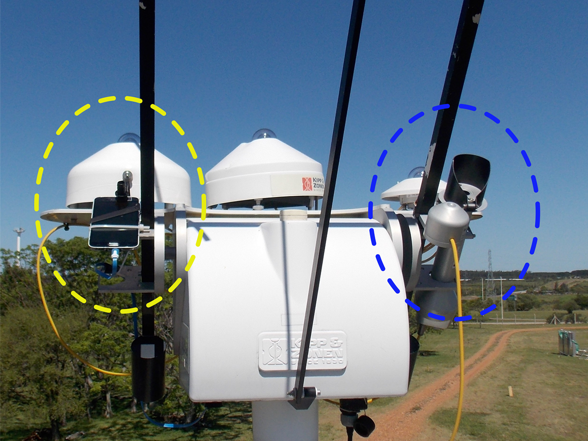
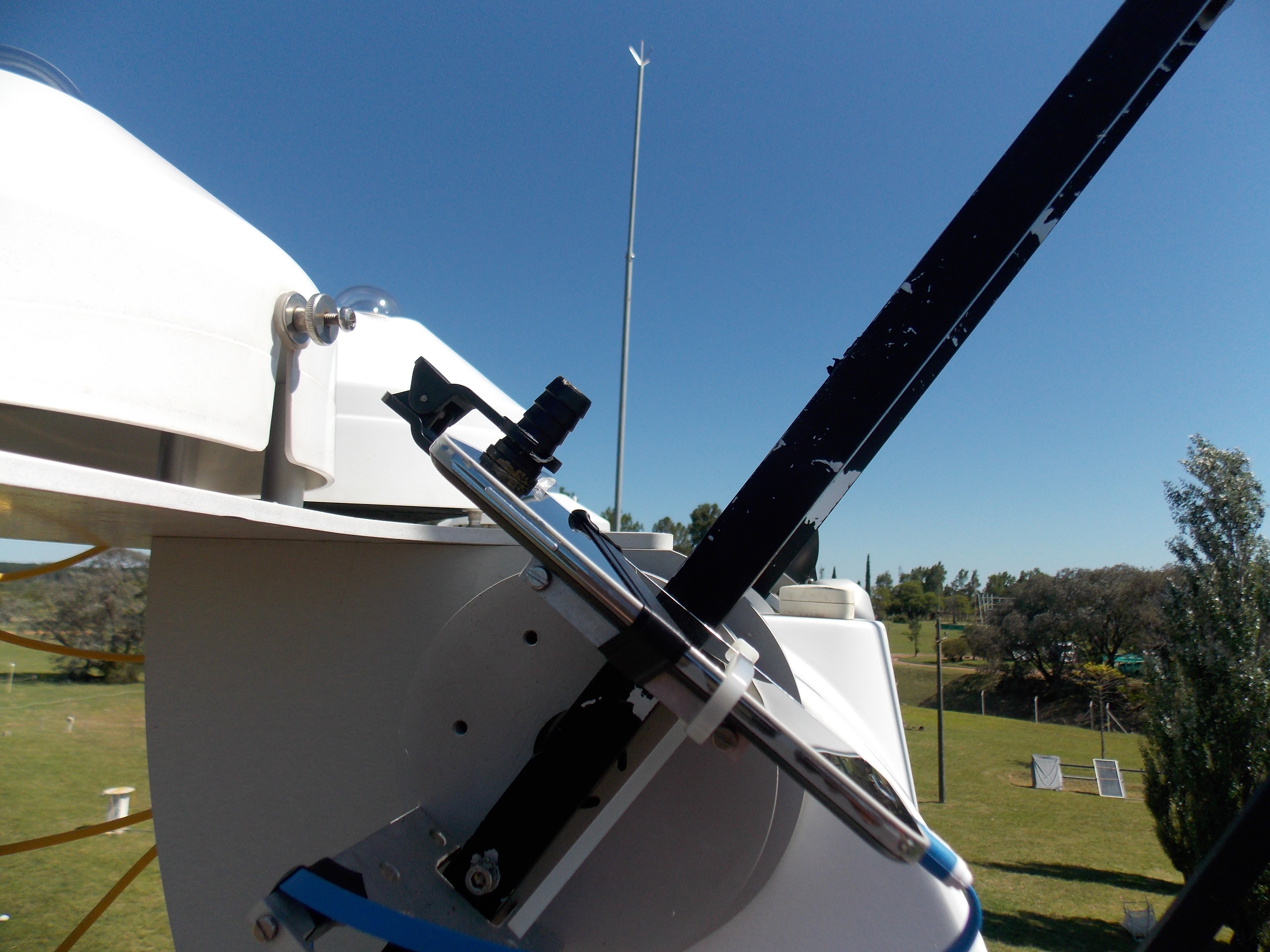
Figure 2: Experimental setup. In the left panel the professional reference equipment (pyrheliometer) and the smartphone can be appreciated. The right panel offers a different perspective of the smartphone alignment.

The measurements were made at the Solar Energy Laboratory (LES) of the University of the Republic (Udelar). The experimental site of this laboratory is located in Salto department, in northwestern Uruguay, with geographic coordinates of $\phi=-31.28^{\circ}$ (latitude) and $\psi=-57.92^{\circ}$ (longitude), corresponding to the UTC-3 time zone. The signal generated by the CHP1 pyrheliometer (in mV) is recorded by a Fisher Scientific DataTaker DT85 data logger and is converted to irradiance (in W/m^-2) through the equipment constant. This measurement is the reference DNI measurement of the LES lab, and it is recorded continuously on a minute scale as an average of instantaneous measurements every 15 s. For the smartphone measurements, the ambient light sensor embedded in the Samsung S5 and the Phyphox [23] application are used. A diffuser is placed above the sensor, in this case, tracing paper printed in black, which prevents saturation of the recorded signal. A cylindrical tube painted black is also placed, which acts as a collimator for a large part of the diffuse irradiance, emulating the professional pyrheliometer collimator (see Fig. 3). Lighting measurements with the light sensor are recorded by the Phyphox app on a minute scale. It can also be on other time scales, for example 5-minute. Once the smartphone is placed in the solar tracker, the collection begins keeping the device measuring during the several hours. To protect the phone screen while the measurements are recorded throughout the day, a double sheet of white paper (A4) placed in front of the smartphone screen, acting as a radiation blocker to prevent the device from overheating as shown in Fig. 3.

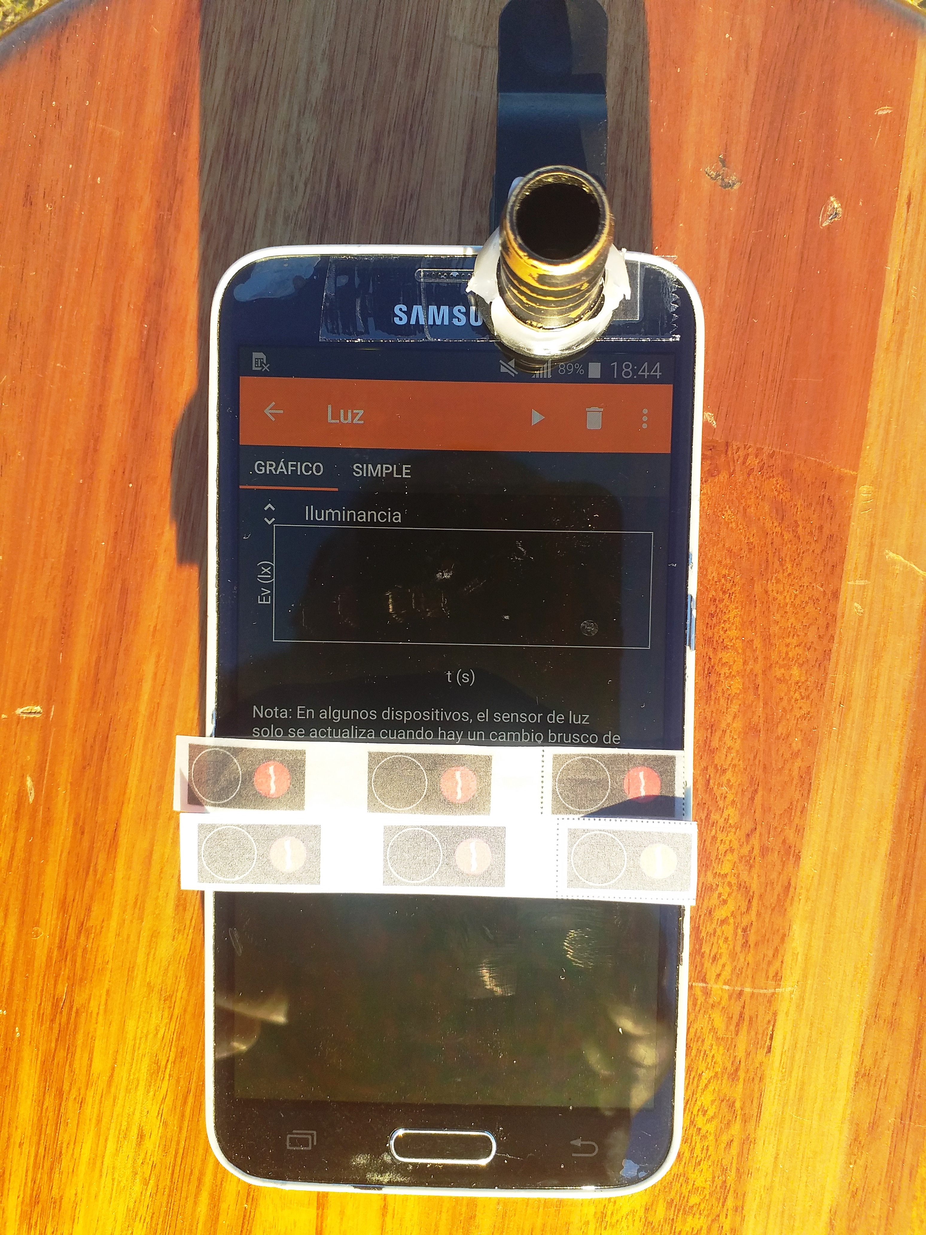
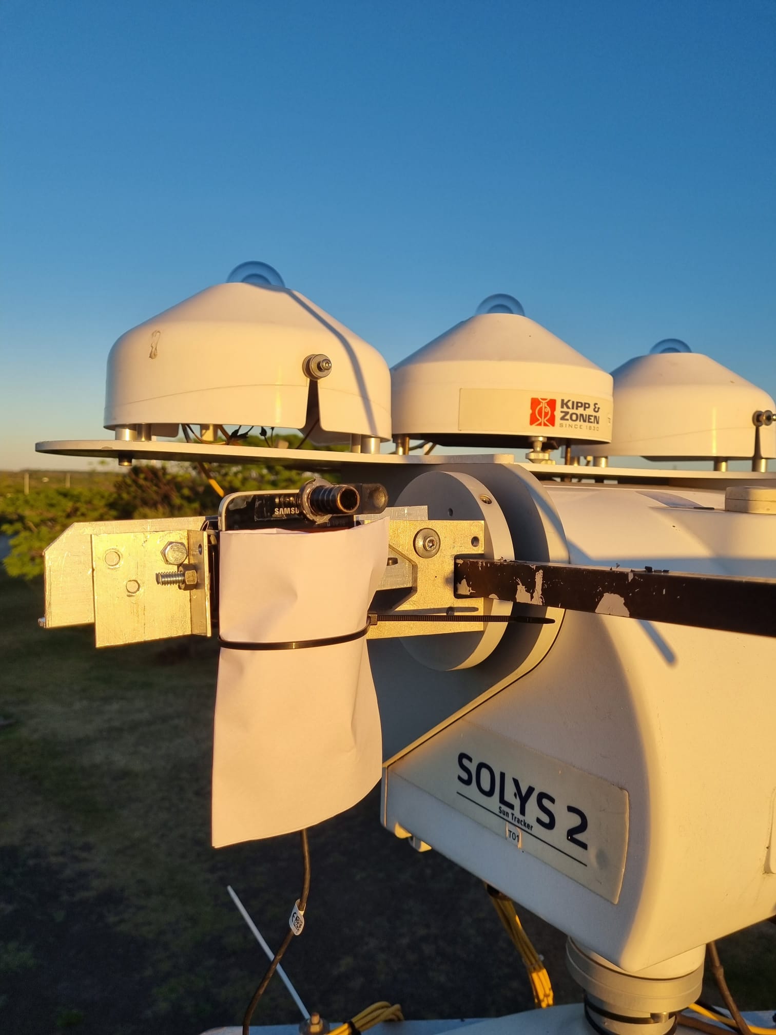
Figure 3: Detailed view of the experimental setup. The left panel exhibits the smartphone and the diffusers while the right panel shows the screen protection used to prevent overheating.

3.2 Practical considerations for the measurements using smartphones

The selection of an appropriate diffuser is crucial in achieving accurate measurements with a smartphone. The smartphone’s analog-digital converter incorporates internal electronics that adjust its gain based on the illuminance detected by the sensor. Consequently, if the solar radiation measurements are low (below $10$ klx, in this case), the equipment will automatically change its scale without notifying the user. Each scale is associated with a specific sensor saturation value, and this scaling behavior can result in erroneous measurements for significant periods when the measurement is in close proximity to the saturation value. Furthermore, for the specific smartphone used in this study, the upper limit of measurable illuminance in the higher range scale is $60$ klx, which represents the saturation threshold. As a point of reference, Michael et al. [24] obtained a conversion constant of $120$ lx / W m^-2, indicating that measuring 1000 W/m² would not be feasible with our smartphone (approximately $120$ klx) without the inclusion of a diffuser. Hence, it is essential to regulate the attenuation of illuminance before it reaches the sensor, for two primary reasons: (i) to ensure that values can be accurately recorded without saturating the sensor, and (ii) to maintain consistent measurements within a specific range of scales at all times. This implies that the introduced attenuation by the diffuser must strike a balance, neither being too minimal nor too excessive, but rather falling within an intermediate range.

To illustrate the impact of different diffusers, we present the results obtained from two clear-sky days using two distinct types of diffusers, as depicted in Fig. 4. The diffusers employed were: (a) ordinary white paper with a surface mass density of 120 g/m², and (b) black printed tracing paper. The graph indicates the illuminance measurements captured by the smartphone (indicated in black) with each diffuser, alongside the reference direct irradiance measurements obtained from the pyrheliometer (displayed in blue), and the clear-sky satellite estimates (depicted in red). The behavior of the measurement obtained using diffuser (a) is illustrated in the left panel of Fig. 4, where the various scale changes occurring at low illuminance levels between $0$ and $5$ klx are clearly observed, along with the corresponding saturation points on each scale. A similar behavior at low illuminance can be observed for diffuser (b) in the right panel of Fig. 4, but only for values below $10$ klx, with notable prominence during sunset. For measurements within the range of values exceeding $10$ klx, the equipment does not undergo scale changes, resulting in continuous and seemingly anomaly-free measurements facilitated by diffuser (b). It is also evident from the graph that the ordinary white paper diffuser attenuates the signal to a greater extent compared to the tracing paper diffuser (as depicted on the right-hand side $y$-axis of both plots). This difference can be attributed to the higher reflectivity of ordinary white paper, particularly within the visible region of the solar spectrum. Therefore, based on our findings, we recommend the use of diffuser (b) in this study. Custom selections may be done for other smartphones, however, this point requires special attention.

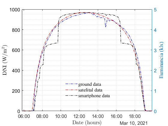
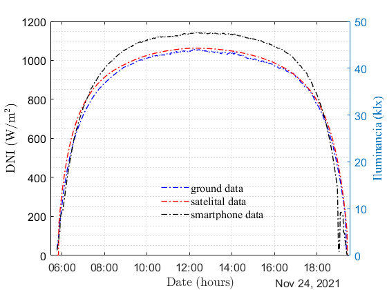
Figure 4: Daily temporal evolution of the direct normal irradiance (DNI) using the smartphone with different diffusers: ordinary white paper (left) and black printed tracing paper (right).

3.3 High precision clear-sky estimates

As an alternative calibration method for places where a professional DNI measurement is not available, it is possible to use as reference accurate clear-sky estimates that use information from weather satellites and physically-consistent atmospheric models. This change in the reference implies a slight increase in the uncertainty in the determination of the calibration constants, since the DNI satellite estimate presents greater uncertainty than a ground reference measurement. There are sophisticated clear-sky models that integrate estimates of different atmospheric variables, either by satellite or by atmospheric reanalysis models, which can be considered as reference [13, 25] if they have been validated by terrestrial measurements with good concordance in various parts of the world.

One interesting choice is the CAMS [26] (Copernicus Atmosphere Monitoring Service) platform which provides free clear-sky estimates using one of these reference models for the entire globe, the McClear model [25]. This model is based on sophisticated radiative transfer calculations from the libRadTran [27] library and its operational version takes the form of a multiple input table based on real-time information on the state of the atmosphere. In particular, this model uses information on aerosols, precipitable water column, and ozone obtained from the CAMS reanalysis database and Earth albedo estimates obtained by the MODIS low-orbit satellite. The CAMS reanalysis in turn assimilates weather satellite’s information to provide its modeled data. Its platform enables access to 1-minute (and other time scales) solar irradiance estimates (global, direct and diffuse) from this high-precision model by simply entering the latitude and longitude of the site of interest. The file header contains information on each of the solar magnitudes provided. For example, the dimensions of radiation are Wh m^-2 (irradiation, energy in the time interval per unit area), which must be converted to W m^-2 (average power per unit area) by the corresponding conversion depending on the time scale.

4 Calibration

After selecting a suitable diffuser (for example the black-printed tracing paper used in this work) we can compare the smartphone illuminance measurements with the DNI data. Here, a calibration function

$$G_{bn}=aE_{v,bn}+b$$ (11)

will be used, where $E_{v,bn}$ is the illuminance measured by the smartphone expressed in klx, $G_{bn}$ are the DNI data expressed in W m^-2, and $a$ and $b$ are two conversion constants to adjust. The calibration is performed with the two reference DNI data sets considered, the professional measurement of the pyrheliometer and the estimates of the McClear model. Minute measurements and estimates of November 24, 2021 were used at the LES experimental site, where clear-sky conditions were maintained throughout the day. Observing the plot of panel b in Fig. 4, for the adjustment we used only the data that meet $E_{v,bn}>15$ klx, so that the smartphone sensor was always on the same scale of measurement. This value was chosen conservatively, in order to ensure measurements at intermediate values on the scale. The calibration constants for both cases are presented in Table 1 and the experimental fit in Fig. 5.

Calibration	Ground	McClear
constant	measurement	estimation
$a$ (W m-2 / klx)	19.29	18.04
$b$ (W m-2)	121.1	193.0
Uncertainty in $a$ (W m-2 / klx)	0.05	0.05
Uncertainty in $b$ (W m-2)	2.2	2.5
Relative uncertainty ($2\sigma$ interval) in $a$	0.54%	0.65%
Relative uncertainty ($2\sigma$ interval) in $b$	3.7%	2.6%

Table 1: Calibration constants from Eq. 11 with different references.

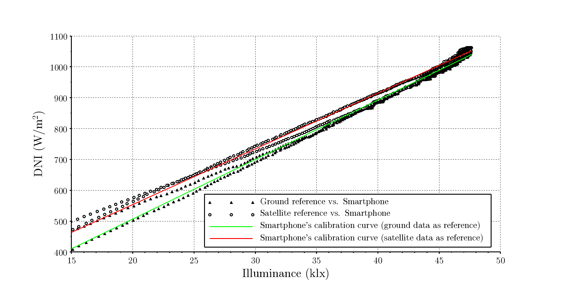
Figure 5: Calibration curves obtained from linear regression between smartphone measurements and reference DNI from terrestrial measurements and from McClear estimates.

Figure 1 reveals that the constants $a$ and $b$ can be determined with low statistical uncertainty for each reference data set (terrestrial measurements and McClear estimates). These uncertainties have been obtained from the linear regression assuming a Gaussian distribution of fluctuations. The table presents the statistical uncertainties in each parameter, both absolute and relative respect to its value, the latter for an interval of $2\sigma$, which approximately represents a confidence level of 95%. For this confidence level, the uncertainty in $a$ is less than 1% and of $b$ less than 4%, for both data sets.

It is interesting to compare the calibration curves. Satellite estimates exhibit deviations from the terrestrial measurements, so the calibration curve based on these data will present more uncertainty than the one obtained by comparison with ground measurements. As observed in Fig. 4, the McClear estimates for that day overestimate the direct irradiance. This leads the calibration curve obtained with this data set results above the calibration curve obtained with terrestrial measurements as observed in Fig. 5. Comparison of the McClear calibration curve with the measured DNI data reports a mean deviation of +2.1% (overestimation) and a mean square deviation of 2.6%. This uncertainty is above the measurement uncertainty of the reference instrument (1%), so it is distinguishable, but at the same time it is below the typical uncertainty of clear-sky satellite models (3-6%) [28]. This demonstrates that it is possible to perform the calibration based on satellite data of solar irradiance with a low uncertainty, enabling its use in the absence of reference measurements. Figure 6 shows the measurements obtained with the smartphone using both calibrations. As can be seen, in both cases a very good DNI measurement is achieved and completely acceptable for an instructional laboratory for a wide range of the day. The only downside is that the smartphone does not achieve a good measurement in the first and last minutes of the day where the illuminance is very low. Outside the diurnal range, i.e. when the sensor measurement is zero, the DNI measurement is affected by the non-zero offset of Eq. 11.

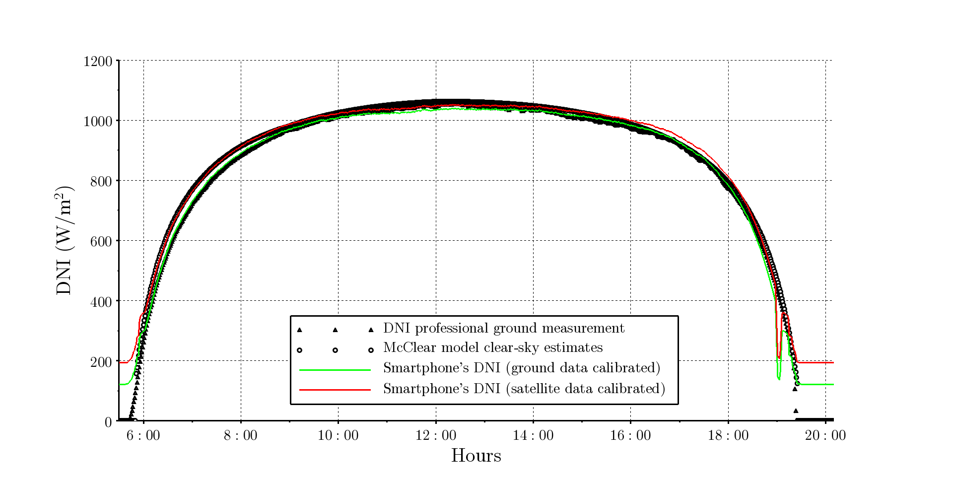
Figure 6: DNI measurements obtained with smartphone on November 24, 2021.

These experimental results reveal that the smartphone is an outstanding tool for measuring solar irradiance through its illuminance sensor, applicable in low-cost university physics laboratories. Furthermore, the measurement capacity achieved with the equipment is really good, even in comparison to commercial sensors. Two relevant questions regarding the measurement capacity of the smartphone arises here. The first is to evaluate the typical uncertainty of a smartphone sensor used to measure DNI with both calibration methods. To answer this question would require data acquisition for several consecutive days (2-3 weeks) similar to professional calibrations following international standards [21]. The second is to evaluate the stability of the calibration curve over time, that is, how robust is the sensor to gradual degradation. This would require a professional calibration of the sensor every 3 months for about a year. With this set of tests it is possible to technically evaluate the capacity limits of the smartphone sensor for the solar irradiance measurement. In fact, moderate-cost professional irradiance sensors are recommended to be calibrated once a year, and a similar recommendation can arise for the smartphone sensor. We recommend here to perform the smartphone calibration each time before its utilization (i.e. the first day of measurements). Similar studies can be carried out for the measurement of global irradiance in the horizontal plane, not only direct irradiance, which surely requires evaluating the non-planar angular response of the smartphone sensor.

5 Instructional laboratory

The preceding section outlined the calibration procedure for transforming a smartphone’s illuminance sensor into a reliable solar irradiance meter, utilizing both high-quality ground measurements and clear-sky satellite estimates. The latter option offers broader accessibility, making it applicable in diverse socio-educational contexts. Once the sensor is appropriately calibrated, it becomes a valuable tool for conducting various solar resource measurements, making it particularly useful in university laboratory settings. The calibrated smartphone can be employed to address numerous aspects related to solar radiation measurement. For instance, it enables the examination of solar resource variations across different geographical locations, under varying cloud conditions, and at different time scales (e.g., throughout a single day, consecutive days, or different seasons). Additionally, by performing measurements over the course of an entire day and integrating the obtained irradiance values, it becomes possible to estimate the daily irradiation. This opens up opportunities for conducting comprehensive analyses of solar radiation characteristics, for example, through a year.

In this section, our focus shifts towards presenting an instructional laboratory that focus into the physics of solar radiation and its interaction with the Earth’s atmosphere. This laboratory is designed around the measurement of a full day using the calibrated smartphone, enabling students to gain a deeper understanding of solar radiation attenuation and its intricate relationship with atmospheric interactions.

The first step consists of calculating the solar trajectory in the celestial sphere for the day in which the measurements will be made in order to know the position to which the smartphone should be tilted. The location of the Sun is determined with the angles of altitude, $\alpha_{s}$, and azimuth, $\gamma_{s}$, calculated by

$$\alpha_{s}=\frac{\pi}{2}-\theta_{z},$$ (12)

and

$$\gamma_{s}=\mathrm{sign}~{}(\omega)~{}\times~{}\left|\arccos\left(\frac{\sin\delta-\cos\theta_{z}\sin\phi}{\sin\theta_{z}\cos\phi}\right)\right|,$$ (13)

As $\phi$ (latitude) is a fixed value and $\delta$ (solar declination) can be considered constant within a day, the intraday variation of these parameters is given by the solar zenith angle, which can be calculated using Eq. 2 based on a time vector specific to the day under consideration. The intraday varying magnitude $\mathrm{sign}~{}(\omega)$ is intended to correct a common sign artifact of the $\arccos$ inverse function, and might not be needed depending on the computing framework. The graph of these two quantities allows to elaborate a solar diagram, as seen in Fig. 7, which illustrates the trajectory of the Sun in the sky for a given day. From this graph it is possible to plan the time to take measurements, for example, by identifying the local time of solar noon (maximum solar height). Additionally, the solar diagram aids in understanding the changing patterns of solar radiation throughout the day.

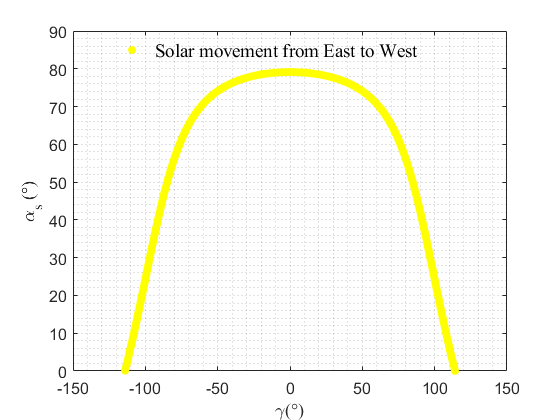
Figure 7: Apparent trajectory of the Sun for November 24, 2021, from East to West, calculated with minute time resolution. Note that the location is in the Southern Hemisphere and the Sun reaches high angles in November.

To conduct the experiment, additional variables need to be obtained, including the orbital factor, the extraterrestrial irradiance corrected by the orbital factor, the air mass (as defined in Eq. 7), and the global optical depth of the Rayleigh extinction (as defined in Eq. 9) for the specific measurement day. While the first two variables exhibit negligible variations within a single day, the latter two vary geometrically throughout the day. To capture these intraday variations, a time vector with minute-scale resolution or 10-minute scale is necessary.

In the subsequent analysis, we will utilize the calibrated measurements obtained from the smartphone over a full day with a minute resolution using the experimental setup illustrated in Fig. 2. In situations where a solar tracking system is not available, the measurements can be performed manually by aligning the smartphone (with the home-made collimator tube attached) towards the Sun and recording measurements at a chosen time interval (such as 10-minute or 15-minute intervals) for a time lapse of 1 to 2 hours centered around solar noon. In this experiment we focused on two activities:

1. Determine the average Linke’s turbidity for the day of measurements, $T_{Lm}$. The instantaneous value of this quantity (in this case, minute) is obtained from Eq. 14. To derive a single daily value of Linke’s turbidity for the entire day or subsequent days, the minute values are averaged around solar noon. This averaging process takes into account the stability of direct radiation during this time period, where its value remains relatively constant, as illustrated in Fig. 4. Therefore, the period around solar noon provides the most favorable conditions for making this determination, ensuring accurate and consistent measurements of turbidity throughout the day.

2. Estimate the DNI for that day with the ESRA model and the estimated local $T_{Lm}$, and compare it to the smartphone ground measurements. This comparison can include the satellite estimates against the device measurement for a comprehensive evaluation of accuracy and reliability.

In the next subsection we conduct a thorough assessment of accuracy and reliability by comparing the smartphone ground measurements with the ESRA model estimation and satellite estimates.

5.1 Determination of the average Linke’s turbidity

The determination of the Linke’s turbidity is based on the smartphone data using the linear relationship given by Eq. 11 averaged around solar noon. In this case, the most reliable linear regression corresponds to the measurements obtained with the reference pyrheliometer. Figure 8 displays the instantaneous values of $T_{L}$ from 10:00 to 15:00 local time. The samples highlighted in red are within $\pm 2$ hours of solar noon for that day (at 12:38). Solar noon’s time can be retrieved from several websites making these kinds of calculations, or by looking the time in which $\cos\theta_{z}$ is maximum (or $w=0$). These samples are used to determine the average value of Linke’s turbidity, $T_{Lm}=2.4$, with a standard deviation of 0.03, which falls within the expected range for a day with high atmospheric clarity.

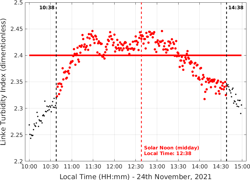
Figure 8: Linke’s turbidity, instantaneous values (points) and averaged (lines). Red points correspond to $\pm 2$ hours of solar noon for that day (at 12:38).

5.2 ESRA model with experimental TL

After determining the average Linke’s turbidity it is possible to estimate the direct irradiance for that day with the ESRA model, according to

$$G_{bn}=G_{sc}F_{n}e^{-2.4\tau_{R}m}.$$ (14)

Figure 9 presents the ground-based DNI measurements, McClear model satellite estimates, and the ESRA model results for the specific day. It is evident that the simplified ESRA model slightly underestimates the clear-sky irradiance for this particular day. On the other hand, the McClear model, which is more complex and incorporates additional atmospheric input information, provides a better fit to the ground measurements, albeit with a slight overestimation. The ESRA model, despite its simplicity, effectively captures the overall behavior of clear-sky irradiance by considering, with only one parameter, various scattering and absorption effects related to solar radiation interaction with different clear-sky atmosphere components (e.g., air, water vapor, aerosols, stratospheric ozone). Considering its performance and ease of implementation, the ESRA model is recommended for inclusion in instructional laboratories about the solar resource. Furthermore, the Linke’s turbidity value can be fairly utilized for subsequent days to assess the behavior of solar irradiance (measured with the calibrated smartphone) in comparison to a clear-sky model adjusted by the students themselves. This allows for the observation and comparison of solar irradiance patterns on different clear-sky days or with varying levels of cloudiness (in cloudy days, for instance, the modeled clear-sky irradiance should be an upper limit of possible irradiance measurements). Additionally, it is possible to quantify the performance of models against ground measurements using the mean deviation and root mean square deviation. In particular, the CAMS website also provides all-sky satellite estimates that can be assessed by students with the calibrated smartphone.

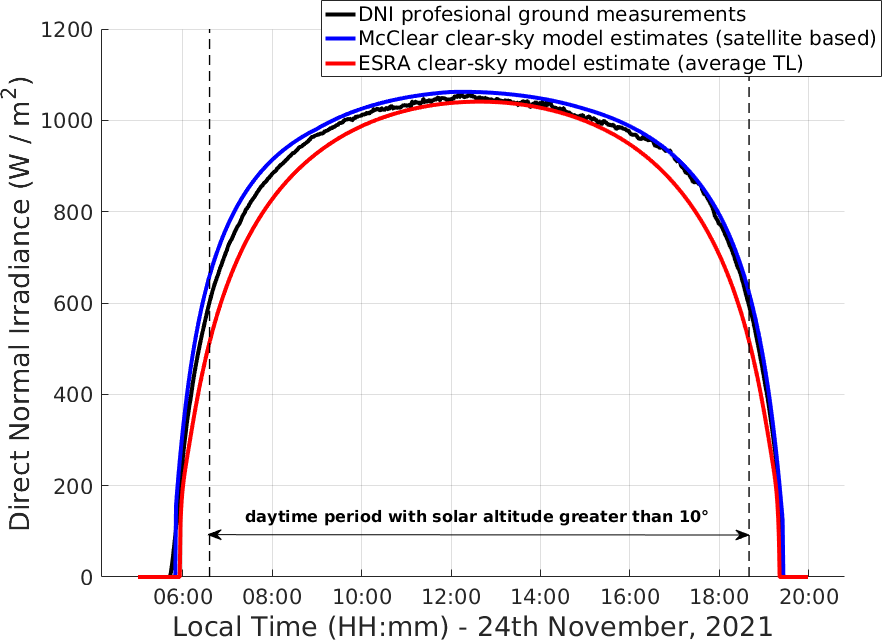
Figure 9: Direct irradiance at normal incidence and clear-sky estimated with the ESRA model and average Linke’s turbidity.

It is common practice to calculate performance indicators by excluding samples with low solar elevations [29, 30] (such as the first and last samples of the day), typically exceeding 5-10 °, as depicted in Figure 9. Alternatively, this threshold could be set with another criterion such as $E_{v,bn}>15$ klx. For instructional purposes, it is recommended to filter samples based on solar elevation ($\alpha_{s}$) and with an exigent criterion, ensuring measurements quality. Table 2 presents the percentage performance metrics using the $\alpha_{s}>10\degree$ guideline. The calculated quantitative indicators for the study day confirm the underestimation of the ESRA model and the slight overestimation of the McClear model, both falling within the $\pm 4$% range. As expected, the relative root mean square deviation (rRMSD) of the ESRA model is higher, but both models exhibit rRMSD values below 5%, which aligns with the expected performance range for clear-sky models.

Model	rMBD (%)	rRMSD (%)
ESRA with averaged Linke’s turbidity.	$-3.7$%	$5.0$%
McClear obtained with CAMS	$+1.8$%	$2.3$%

Table 2: Performance indicators of the two clear-sky models considered here compared to calibrated smartphone ground measurements (using professional pyrheliometer reference).

6 Conclusion

This study reveals the remarkable potential of smartphone light sensors as effective tools for measuring direct solar irradiance and for introducing students to the fundamental aspects of the solar resource within instructional laboratories. The proposed experiment involves aligning the equipment with the Sun at all times using a home-made collimator tube, thereby allowing to focus on the smartphone’s ability to measure irradiance without considering geometrical and optical aspects that influence other solar irradiance measurements (i.e. global horizontal). In terms of equipment positioning while this study employed a professionally precise solar tracker to gather continuous measurements throughout the day, for instructional laboratory purposes students can manually perform measurements at regular intervals throughout a day. This modification enables hands-on student engagement and participation.

Two calibration methods were presented to convert smartphone illuminance measurements into solar irradiance: comparison with a reference measurement and utilization of clear-sky satellite estimates, which are readily available for any location on the globe (the McClear model). Remarkably, this work demonstrated that calibration against both data sets can be performed without introducing a significant increase in uncertainty, resulting in highly reliable measurement capabilities suitable for instructional laboratories. It is crucial to conduct calibration on a clear-sky day, following the same principles applied in professional calibrations according to current ISO standards for commercial radiometers. The findings of this study pave the way for the development of various low-cost instructional laboratories, both within traditional classroom settings and in outdoor environments. In the process, students must learn to develop important scientific-mathematical skills such as the recording and processing of experimental data, assess their quality with or without data filtering, and assigning uncertainty to simplified models for direct solar irradiance estimation at ground level. Moreover, the calibration process itself allows students to be introduced to simple linear regression, and the uncertainty assignment to its parameters and the final result.

This work shows that smartphones are a high-potential measurement and learning tool, as well as a laboratory in the pocket of every citizen, also on issues related to solar energy. This is a current and relevant topic to be introduced in scientific-technological university careers, given the energy transition that humanity must go through in the coming decades from a high energy dependence on fossil fuels towards renewable energies. The demonstration that smartphones are capable of measuring solar irradiance with low uncertainty and reporting verifiable results with professional measurements and estimates, opens up several didactic possibilities and future studies. To mention a few, it is possible to consider the measurement of global irradiance (direct + diffuse) in a horizontal plane and analyze the directional response of the smartphone sensor, carry out studies to assign a typical measurement uncertainty to the equipment in relation to professional equipment and/or study the behavior of the sensor spectra, using spectral measurements of solar irradiance. By leveraging smartphone technology, students can gain practical insights into solar irradiance measurement, fostering a deeper understanding of this important aspect of renewable energy resources.

Data availability

The data that support the findings of this study are available on reasonable request.

References

References

- [1] BP 2021 Statistical Review of World Energy URL http://bp.com/statisticalreview
- [2] REN21 2021 Renewables 2021: Global Status Report URL http://www.ren21.net
- [3] Monteiro M and Martí A C 2022 American Journal of Physics 90 328–343
- [4] Gil S and Di Laccio J 2017 Lat. Am. J. Phys. Educ. 11 1305(1–9)
- [5] Monteiro M, Stari C, Cabeza C and Martí A C 2021 American Journal of Physics 89 477–481 ISSN 0002-9505 URL https://doi.org/10.1119/10.0002906
- [6] Monteiro M, Stari C, Cabeza C and Martí A C 2017 The Physics Teacher 55 264–266
- [7] Fröhlich C 2006 Space Science Reviews 125 53––65
- [8] Kopp G and Lean J 2011 Geophysical Research Letters 38 L01706
- [9] Iqbal M 1983 An Introduction to Solar Radiation (Toronto: Academic Press) ISBN 0-12-373752-4
- [10] Duffie J A and Beckman W A 2013 Solar Engineering of Thermal Processes 4th ed (John Wiley and Sons, Inc.) ISBN 9780470873663
- [11] Spencer J 1971 Search 2 172 (Preprint http://mail-archive.com/sundial@uni-koeln.de/msg01050.html)
- [12] Kasten F and Young A T 1989 Applied optics 28 4735–4738
- [13] Gueymard C A 2008 Solar Energy 82 272–285 ISSN 0038-092X URL http://www.sciencedirect.com/science/article/pii/S0038092X07000990
- [14] Oumbe A, Qu Z, Blanc P, Lefèvre M, Wald L and Cros S 2014 Geoscientific Modeel Development 7 1661–1669
- [15] Gueymard C A 2012 Solar Energy 86 2145–2169 ISSN 0038-092X progress in Solar Energy 3
- [16] Rigollier C, Bauer O and Wald L 2000 Solar Energy 68 33–48 ISSN 0038-092X
- [17] Kasten F 1984 Ann. der Meteorol 20 49–50
- [18] Louche A, Peri G and Iqbal M 1986 Solar Energy 37 393–396
- [19] Grenier J, De La Casinére A and Cabot T 1994 Solar Energy 52 303–313
- [20] Kasten F 1996 Solar Energy 56 239–244
- [21] ISO 9847:1992 1992 Solar energy — calibration of field pyranometers by comparison to a reference pyranometer https://www.iso.org/standard/17725.html
- [22] Zonen K 2020 CHP1 Pyrheliometer https://www.kippzonen.com/Product/18/CHP1-Pyrheliometer
- [23] University R A 2020 phyphox, physical phone experiments https://phyphox.org/
- [24] Michael P R, Johnston D E and Moreno W 2020 Journal of Measurements in Engineering 8 153–166
- [25] Lefèvre M, Oumbe A, Blanc P, Espinar B, Qu Z, Wald L, Homscheidt M S and Arola A 2013 Atmospheric Measurement Techniques, European Geosciences Union 6 2403–2418
- [26] Programme T C 2020 Atmosphere Monitoring Service (CAMS) http://www.soda-pro.com/web-services/radiation/cams-radiation-service
- [27] Mayer B and Kylling A 2005 Atmospheric Chemistry and Physics 5 1855–1877
- [28] Laguarda A, Giacosa G, Alonso-Suárez R and Abal G 2020 Solar Energy 199 295–307 ISSN 0038-092X
- [29] Yang D and Bright J M 2020 Solar Energy 210 3–19 ISSN 0038-092X special Issue on Grid Integration URL https://www.sciencedirect.com/science/article/pii/S0038092X20303893
- [30] Laguarda A, Alonso-Suárez R and Abal G 2023 Solar Energy 259 30–40 ISSN 0038-092X URL https://www.sciencedirect.com/science/article/pii/S0038092X23002864