MDTD: A Multi-Domain Trojan Detector for
Deep Neural Networks

Abstract.

Machine learning models that use deep neural networks (DNNs) are vulnerable to backdoor attacks. An adversary carrying out a backdoor attack embeds a predefined perturbation called a trigger into a small subset of input samples and trains the DNN such that the presence of the trigger in the input results in an adversary-desired output class. Such adversarial retraining however needs to ensure that outputs for inputs without the trigger remain unaffected and provide high classification accuracy on clean samples. Existing defenses against backdoor attacks are computationally expensive, and their success has been demonstrated primarily on image-based inputs. The increasing popularity of deploying pretrained DNNs to reduce costs of re/training large models makes defense mechanisms that aim to detect ‘suspicious’ input samples preferable.

In this paper, we propose MDTD, a Multi-Domain Trojan Detector for DNNs, which detects inputs containing a Trojan trigger at testing time. MDTD does not require knowledge of trigger-embedding strategy of the attacker and can be applied to a pretrained DNN model with image, audio, or graph-based inputs. MDTD leverages an insight that input samples containing a Trojan trigger are located relatively farther away from a decision boundary than clean samples. MDTD estimates the distance to a decision boundary using adversarial learning methods and uses this distance to infer whether a test-time input sample is Trojaned or not.

We evaluate MDTD against state-of-the-art Trojan detection methods across five widely used image-based datasets- CIFAR100, CIFAR10, GTSRB, SVHN, and Flowers102, four graph-based datasets- AIDS, WinMal, Toxicant, and COLLAB, and the SpeechCommand audio dataset. Our results show that MDTD effectively identifies samples that contain different types of Trojan triggers. We further evaluate MDTD against adaptive attacks where an adversary trains a robust DNN to increase (decrease) distance of benign (Trojan) inputs from a decision boundary. Although such training by the adversary reduces the detection rate of MDTD, this is accomplished at the expense of reducing classification accuracy or adversary success rate, thus rendering the resulting model unfit for use.

1. Introduction

Advances in cost-effective storage and computing have resulted in the widespread use of deep neural networks (DNNs) to solve complex tasks. Examples of such tasks include image classification (Yu et al., 2018), text generation (Zhu et al., 2018), and safety-critical applications such as autonomous driving (Grigorescu et al., 2020). However, training such large models requires significant computational resources, which may not be available to most DNN users. Two approaches that have been proposed to overcome the challenge of significant computational resources required to train such models are (i) using publicly shared pre-trained DNN models (Kurita et al., 2020) and (ii) training large models on online machine learning platforms (AWS, 2018; Big, 2018; Caf, 2018). However, when the end-user of a DNN is different from the entity that trained the model (e.g., in online ML platforms), it is possible for an adversary to launch adversarial attacks such as a backdoor attack (Li et al., 2022) and share the defective model for use by the public.

BadNets	Nature	Blend	SQ	WM	L2 inv

Figure 1. (Top Row) Different types of Trojan triggers that we examine for inputs from the CIFAR10 dataset that consists of $10$ classes. (Bottom Row) Image of a bird (Class 2) embedded with the trigger. After the DNN identifies the bird embedded with a trigger as a frog (Class 6).

An adversary carrying out a backdoor attack inserts a predefined perturbation called a trigger into a small set of input samples (Li et al., 2022). The DNN models can then be trained so that the presence of the trigger in an input will result in an output label that is different from the correct output label (an existing class or a completely new class not known to the user (Li et al., 2022)). Adversarial training also ensures that output labels corresponding to clean inputs (inputs without the trigger) remain unaffected. A DNN model that misclassifies inputs that contain a trigger is termed Trojaned. Backdoor attacks are highly effective when only classification output labels of models are available to the users. In (Gu et al., 2019), DNN models used in autonomous driving applications were shown to incorrectly identify a STOP sign with a small sticker on it (the trigger) as a ‘speed limit’ sign. Backdoor attacks with different types of triggers embedded in inputs from the CIFAR10 dataset are illustrated in Fig. 1.

Defenses against backdoor attacks involve (i) pruning or retraining the DNN (e.g., Fine-Pruning (Liu et al., 2018a)), (ii) developing Trojan model detectors (e.g., Neural Cleanse (Wang et al., 2019)) to detect an embedded backdoor, or (iii) detecting Trojan samples at inference (Gao et al., 2019) or training time (Tran et al., 2018). Performance of these methods were examined and reported to be computationally expensive in (Li et al., 2022) (Sec. VIII). These methods also assume that the user of the model has adequate resources to (re)train the DNN model (Liu et al., 2018a; Tran et al., 2018) or identify and reconstruct an embedded trigger (Wang et al., 2019). These challenges underpin a need to develop mechanisms to effectively detect input samples that have been embedded with a Trojan trigger and discard such inputs before they can be provided to a DNN model.

In this paper, we propose MDTD, a mechanism to detect Trojan samples that uses a distance-based reasoning to overcome the challenges listed above. MDTD is a computationally inexpensive inference-time detection mechanism that can be applied to pre-trained DNN models. MDTD does not aim to inspect and remove an embedded backdoor from the given DNN model; rather, it determines if an input sample to the given DNN contains a trigger with high probability, and discards such inputs. The effectiveness of MDTD is underscored by the fact that it is agnostic to the specific trigger-embedding strategy employed by the adversary.

MDTD uses the insight that samples containing a Trojan trigger will typically be located farther away from the decision boundary compared to a clean sample. Consequently, a larger magnitude of noise will need to be added to a Trojaned sample to move it across the decision boundary so that it will be misclassified by the DNN. Since it makes use of the distance metric from a decision boundary, MDTD is applicable to different input data modalities.

We illustrate the insight and motivation behind MDTD using t-SNE visualization techniques (Van der Maaten and Hinton, 2008) to demonstrate that embedding of a Trojan trigger can be qualitatively examined through the lens of feature values at intermediate DNN layers. To quantitatively verify this insight, we compare distances of clean and Trojan samples to a decision boundary using the notion of a certified radius (Cohen et al., 2019). However, computing the certified radius can incur large costs (Li et al., 2023). To overcome this challenge, MDTD estimates the distance of Trojan and clean samples from a decision boundary using adversarial learning (Goodfellow et al., 2015) in a computationally efficient manner. MDTD then determines a threshold on the computed distance using only a small number of clean samples without making any assumption about the adversary’s trigger-embedding strategy. Our contributions are:

• We propose MDTD, a practical framework to detect Trojaned inputs in image, graph, and audio-based input domains in a computationally inexpensive manner.

• We demonstrate the effectiveness of MDTD through comprehensive evaluations and comparisons with state-of-the-art (SOTA) Trojan input detection methods for different types of Trojan triggers across five image-based input datasets: CIFAR100, CIFAR10, GTSRB, SVHN, and Flowers102.

• We examine the performance of MDTD on four graph-based input domains: AIDS, WinMal, Toxicant, and COLLAB and one audio dataset SpeechCommand.

• We evaluate MDTD against adaptive Trojan trigger-embedding attacks where the adversary has complete knowledge about the details of MDTD-based detection and aims to construct new Trojan trigger embeddings to bypass detection. We empirically show that although such retraining of the DNN reduces the detection rate of MDTD, it simultaneously lowers classification accuracy of the DNN on clean samples below $50\%$, thus making the DNN unfit for use.

Sec. 2 provides background on DNNs and backdoor attacks. Sec. 3 describes our threat model, and Sec. 4 specifies assumptions on user capability. We motivate and describe the design of MDTD in Sec. 5. We evaluate MDTD in Sec. 6 and discuss MDTD in Sec. 7. Sec. 8 presents related work and Sec. 9 concludes the paper.

2. Preliminaries

This section gives an overview of deep neural networks (DNNs), graph neural networks (GNNs), and long-short-term-memory (LSTM) models. We describe how an adversary can carry out a backdoor attack on these models, and specify metrics to evaluate effectiveness of the attack and our proposed defense MDTD.

2.1. DNNs and Backdoor Attacks

Deep neural networks (DNNs) are complex machine learning models (ML) developed for tasks with high-dimensional input spaces (e.g., image classification, text generation) (Goodfellow et al., 2016). These models take an input $x$, compose $x$ through layers ($f(x):=l_{1}\circ l_{2}\circ\cdots\circ l_{k}(x)$), and return output $y$. For e.g., in image classification, $x\in[0,1]^{(W\times H)}$ is an image, and the DNN returns an output $y\in\{1,\cdots,C\}$ where $W\times H$ is the resolution of $x$ and $C$ is the number of classes.

DNN models for classification tasks are known to be vulnerable to backdoor attacks (Li et al., 2022). An adversary carrying out a backdoor attack can retrain a DNN to return a different output label when a trigger is embedded into the input sample, while recognizing clean samples correctly. An adversary can carry out a backdoor attack by embedding triggers into a subset of samples in the training data (Gu et al., 2019; Chen et al., 2017) or manipulating weights in layers of the DNN (Li et al., 2019) to induce erroneous behavior at test time for inputs that contain the trigger. For e.g., in image classification using the CIFAR10 dataset (Fig. 1), the adversary manipulates the model $f$ to return a desired label corresponding to frog (Class 6) that is different from the true label of bird (Class 2) for inputs that contain a predefined trigger.

2.2. GNNs and Backdoor Attacks

Graph neural networks (GNNs) are a class of deep learning models designed to make inferences on graph-based data (Hamilton, 2020). The input to a GNN is a graph $\mathcal{G}=(V,E)$ where $V$ is the set of individual nodes, and $E$ is the set of edges between pairs of nodes. Each node $v\in V$ has an associated set of $d$ features, denoted $x_{v}\in\mathbb{R}^{d}$. We let $X\in\mathbb{R}^{|V|\times d}$ be the feature representation matrix associated with graph $\mathcal{G}$. In this paper, we focus on a recently proposed backdoor attack on GNNs that use a message passing paradigm (Hamilton et al., 2017), and graph classification tasks where the goal is to predict the class that an input graph belongs to. Under the message passing paradigm, at each iteration $t$, $x_{v}$ is updated as follows: $x^{(t)}_{v}=\mathcal{U}(x^{(t-1)}_{v},\mathcal{A}({x^{(t-1)}_{u},\forall u\in\mathcal{N}(v)}))$, where $\mathcal{N}(v)$ is the set of neighbours of $v$, $\mathcal{A}$ is an aggregate function that takes the feature representations of each node from $v$’s neighbors as input, and  $\mathcal{U}$ is an update function that takes $x_{v}$ at iteration $(t-1)$ and the output of the aggregate function $\mathcal{A}$ as inputs. After $T$ iterations, individual node representations are pooled to generate a graph representation $x_{\mathcal{G}}=f(\mathcal{G},X)$. The graph classification task can then be expressed as $h:f(\cdot,\cdot)\rightarrow\{1,2,\dots,C\}$.

An attacker carrying out a backdoor attack on GNNs uses a subgraph (a subset of vertices and edges associated to vertices) of $\mathcal{G}$ as the trigger. We adopt the Graph Trojan Attack (GTA) proposed in (Xi et al., 2021) to generate Trojaned GNN models. GTA uses trigger-embedded graphs to update GNN parameters. The updated GNN model is passed to a trigger generation network which generates the trigger for the next iteration of the message passing procedure. The trigger generation network consists of a topology generator that updates the subgraph, and a feature generator that updates features associated to nodes in the Trojaned subgraph. The goal of the adversary is to ensure that the Trojaned GNN model returns a desired label $y^{d}$ that is different from the true label for graph inputs that are embedded with the predefined ‘triggered’ subgraph.

2.3. Audio Models and Backdoor Attacks

Long-Short-Term-Memory (LSTM) models enable processing and reasoning about sequences of information, e.g., in audio and speech processing (Warden, 5 11). We use an LSTM combined with a DNN model to train an audio classifier. The model takes an audio input $x^{1\times H}$, and returns an output $y\in\{1,\cdots,C\}$, where $1\times H$ is the resolution of $x$ and $C$ is the number of classes. An audio input is comprised of a set of frequencies, which could be different for each input.

For a sample audio $x$, its Trojaned version $x_{T}$ can be generated using two different backdoor attacks: (i) Modified, where a small part of the audio was replaced by an arbitrary (but fixed) audio noise pattern, and (ii) Blend, where a randomly generated (but fixed) audio noise trigger was mixed into a part of the audio. Specifically, at time-interval $[i,i+w]$, $x_{T}[i:i+w]=(1-\alpha)\times x[i:i+w]+\alpha\times Trigger$, where $\alpha=1$ for Modified, and $\alpha\in[0.05,0.2]$ for Blend.

2.4. Metrics

We describe metrics used to evaluate backdoor attacks and Trojan sample detection methods. We assume that defense mechanisms return a positive label if they identify a sample as Trojan. In the literature (James et al., 2013), such positive identification of the Trojan is called a true positive rate. SImilarly, when the defense mechanism incorrectly labels a clean sample as Trojan, it is called a false positive or false alarm. We now define suitable metrics below:

True Positive Rate (TPR) is the fraction of Trojan samples that received a positive label.

False Positive Rate (FPR) is the fraction of clean samples that incorrectly received a positive label (raising a false alarm).

$F_{1}$-score: An effective Trojan detection method has a high detection accuracy (TPR) and low false alarm (FPR). Defining $TNR=1-FPR$, the $F_{1}$-score combines $TPR$ and $TNR$ as:

(1) $$F_{1}=\frac{2*TPR*TNR}{TPR+TNR}.$$

The $F_{1}$-score is widely used to compare Trojan detection methods, and a higher $F_{1}$-score indicates a better detector (Chen et al., 2018).

Attack Success Rate (ASR) is the fraction of Trojan samples that result in the DNN model returning the attacker’s desired output (Li et al., 2022).

3. Threat Model

In this section, we introduce the threat model we consider, and describe our assumptions on capabilities of the attacker.

Adversary Assumptions: We assume that the adversary has access to a pretrained model and adequate data is available such that a subset of these samples can be used by the adversary to embed a Trojan trigger into them. The adversary is also assumed to have sufficient computational resources required to (re)train the DNN using both, the Trojan trigger-embedded and clean samples.

Adversary Goals and Actions: The adversary’s aim is to use Trojan-embedded as well as clean samples to train a Trojaned DNN model such that: (i) for Trojan trigger-embedded inputs, the output of the DNN is an adversary-desired target class, which may be different from the true class, and (ii) for clean inputs, the classification accuracy is as close to the accuracy of the un-Trojaned DNN.

Performance Metrics: Performance metrics defined in Sec. 2.4, including the true/ false positive rates, and the attack success rate (ASR) can be computed by the adversary after it trains the Trojaned DNN model. We use these metrics to characterize and empirically evaluate the effectiveness of an attack. The objective of the adversary is typically to ensure that the value of ASR is high, while the $F_{1}$-score in our context, which quantifies the defender’s ability to detect a sample containing a Trojan trigger is as small as possible.

The adversary is assumed to perform trigger embedding in a stealthy manner such that its specific attack strategy and parameters, including the nature and location of the Trojan triggers embedded in the sample, as well as information about data samples that have been embedded with Trojan triggers is not revealed.

CIFAR100
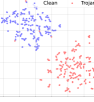
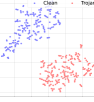
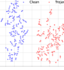
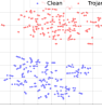
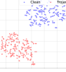
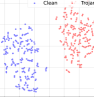
CIFAR10
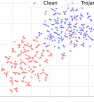
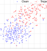
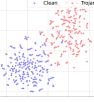
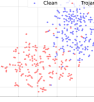
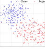
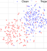
GTSRB
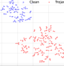
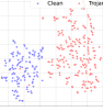
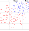
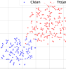
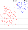
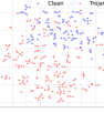
SVHN
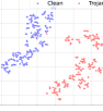
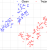
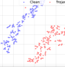
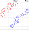
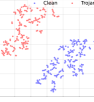
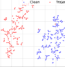
Flower102
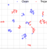
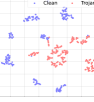
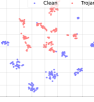
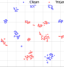
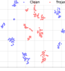
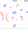
	BadNets	Blend	Nature	Trojan SQ	Watermark	L2 inv

Figure 2. This figure shows t-SNE visualizations for outputs of the penultimate layer of the DNN for $200$ clean samples (blue dots) from the target class (Class 6) and $200$ Trojaned samples (red dots) misclassified to the target class. We examine the CIFAR10, CIFAR100, GTSRB, SVHN, and Flower102 datasets, and six Trojan triggers (Badnets, Blend, Nature, Trojan SQ, Trojan WM and L2 inv) for each dataset. In most cases, we observe that although the DNN classifies both clean and Trojaned samples to the same class (Class 6), it generates different values for features in its penultimate layer. Embedding a trigger into samples from CIFAR10 and GTSRB using the L2 inv trigger is relatively less easy (compare separability of blue and red dots in Col 6, Row 2 and Col 6, Row 3).

4. User Capability

The user has limited computational resources, and uses ML platforms to train a model or uses publicly available models which have high accuracy on clean samples. However, the user has sufficient resources to use an adversarial learning method (Goodfellow et al., 2015) to obtain the magnitude of adversarial noise that will result in misclassification of an input sample. We further assume that the user is aware of the possibility that the input sample or the model can be Trojaned, and aims to detect and remove malicious inputs. However, the user has no knowledge of the attacker strategy, and identities of the Trojan trigger and target class. The user is assumed to have access to a set of clean samples whose labels are known. The user has either white-box access (access to weights and hyperparameters of the DNN model) or black-box access (access to only outputs of the DNN model). We note that developing solutions for black-box model access is more difficult than for the white-box setting, where information about the DNN model is available. For both settings, our objective is to develop a method that would aid a user in identifying and discarding input samples that contain a Trojan trigger.

5. MDTD: Motivation and Design

Table 1. This table reports average (standard deviation) of certified radii for $200$ clean and $200$ Trojan samples for the CIFAR10, CIFAR100, GTSRB, and Flower102 datasets with six different Trojan triggers (noted in bold column titles). We observe that Trojan samples have a higher average certified radius than clean samples. Thus, the minimum magnitude of noise required to make a DNN model misclassify an input sample containing a Trojan trigger is larger.

Dataset	Clean	Badnets	Blend	Nature	Trojan SQ	Trojan WM	L2 inv
CIFAR100	0.005 (0.045)	0.657 (0.132)	0.103 (0.131)	0.880 (0.017)	0.759 (0.047)	0.893 (0.0001)	0.596 (0.036)
CIFAR10	0.015 (0.046)	0.875 (0.035)	0.308 (0.216)	0.893 (0.000)	0.893 (0.0001)	0.893 (0.0001)	0.648 (0.059)
GTSRB	0.308 (0.326)	0.663 (0.234)	0.749 (0.227)	0.882 (0.068)	0.857 (0.106)	0.499 (0.235)	0.239 (0.148)
SVHN	0.255 (0.268)	0.727 (0.178)	0.651 (0.271)	0.887 (0.035)	0.879 (0.083)	0.882 (0.062)	0.893 (0.0001)
Flower102	$0.038(0.173)$	$0.189(0.163)$	$0.634(0.302)$	$0.875(0.07)$	$0.893(0.001)$	$0.893(0.001)$	$0.269(0.148)$

In this section, we describe the mechanism of MDTD. We motivate the development of MDTD by showing that feature values at intermediate layers of the DNN corresponding to clean and Trojaned samples are different. We hypothesize that as a consequence, clean and Trojaned samples will behave differently when perturbed with noise, and use the notion of a certified radius (Cohen et al., 2019) to verify this. We then explain how MDTD computes an estimate of the certified radius to effectively distinguish between Trojan and clean samples.

5.1. Key Intuition behind MDTD

Feature Value Visualization using t-SNE: For a DNN model with $K$ layers, the first $(K-1)$ layers map an input $x$ to the feature space, which typically has a lower dimension than the high-dimensional input space. The last layer of the DNN then uses the values in the feature space to make a decision about the input. For example, in an image classification task, the decision will be the identity of the class that the input is presumed to belong to. Thus, the output of the penultimate layer (layer $K-1$) of the DNN can then be interpreted as an indicator of the perspective of the DNN about the given input sample.

We use a t-distributed stochastic neighbor embedding (t-SNE) (Van der Maaten and Hinton, 2008) to demonstrate that for the same output of the DNN model, values in the feature space for clean and Trojan samples are different. The t-SNE is a technique to visualize high-dimensional data through a two or three dimensional representation. For the CIFAR10, CIFAR100, GTSRB, SVHN, and Flowers102 datasets, we collect $200$ samples corresponding to each of six different Trojan trigger types that are classified by the DNN model as belonging to the class $y^{d}=6$ due to the presence of the trigger. We additionally collect $200$ clean input samples that do not contain a Trojan trigger for whom the output of the DNN model is $y=y^{d}$.

Fig. 2 shows t-SNE representations of the feature values of these samples, i.e., the outputs at the penultimate layer of the DNN. We observe that the clean samples (blue dots) can be easily distinguished from Trojan samples (red dots) for each of the Trojan trigger type in all five datasets. While the t-SNE visualization provides qualitative indicators of clean and Trojaned sample behavior, we are also interested in quantitative metrics. We use the certified radius to distinguish between clean and Trojaned input samples.

Certified Radius: The certified radius is defined (Cohen et al., 2019) as the radius of the largest ball centered at each input sample within which the DNN model returns the same output label. The certified radius is computed by estimating the distance to a decision boundary by perturbing samples with Gaussian noise with a predetermined/ known mean and variance. However, exactly computing the certified robustness has a high computational cost (Li et al., 2023). Instead, we evaluate the robustness of Trojan-embedded samples by approximately computing the certified radius using a heuristic that perturbs a small number of clean and Trojaned samples with Gaussian noise centered at the input sample of interest.

Table 1 presents average certified radii for $200$ clean and $200$ Trojan samples with six different Trojan trigger types (Badnets, Blend, Nature, Trojan SQ, Trojan WM and L2 inv) applied on CIFAR10, CIFAR100, GTSRB, SVHN and Flowers102 datasets. We observe that the certified radius is significantly higher for Trojaned samples than for clean samples, clearly indicating a relatively larger distance to the decision boundary. Consequently, the minimum magnitude of noise required to make the DNN misclassify a Trojan sample will be larger than the noise required to misclassify a clean sample.

Although t-SNE visualizations and certified radius computation provide preliminary insights into differences between clean and Trojan samples, there are two significant challenges which limit their direct use in Trojan trigger detection. First, while t-SNE provides visual insights, it relies on access to (i) adequate number of clean and Trojan trigger-embedded samples, and (ii) outputs at intermediate layers of the DNN. However, t-SNE visualizations are not useful as a direct computational mechanism for Trojan detection since the user of a DNN model will typically not have access to adequate number Trojan trigger-embedded samples. Further, access to intermediate layers is not feasible for users who only have black-box model access (i.e., access to only outputs of the model). Second, computing the certified radius is computationally expensive, and is known to be NP-complete (Li et al., 2023), which limits their use in practice. We next present a two-stage algorithmic design for MDTD that leverages insights from t-SNE visualizations and certified radii.

5.2. Two-Stage Design of MDTD

MDTD makes use of adversarial learning techniques (Goodfellow et al., 2015) to estimate distance of a sample from any decision boundary. It then computes the smallest magnitude of adversarial noise required to misclassify the sample to infer whether the sample is Trojaned or not. MDTD consists of two stages. In the first stage, MDTD estimates the distance of a given input sample to the decision boundary. In the second stage, distances estimated in the previous step and the distance of a small number of clean samples to the decision boundary are used to identify whether the sample contains a Trojan trigger or not. We describe each stage below.

Stage 1: Estimating distance to decision boundary: MDTD uses adversarial learning techniques (Goodfellow et al., 2015; Moosavi-Dezfooli et al., 2017) to estimate the minimum magnitude of noise perturbation, denoted $\delta$, that will cause the DNN model to misclassify a given sample. For an input sample $x$, the output of the DNN model is denoted $f(x)$. The value of the smallest perturbation $\delta$ is obtained by maximizing a loss function $\mathcal{L}(\cdot,\cdot)$ that quantifies the difference between the output label of the DNN for a perturbed variant of the input, denoted $f(x+\delta)$, and the true label of the input $y$. This objective is well-defined and can be expressed as a regularized optimization problem with regularization constant $\lambda$ as (Goodfellow et al., 2015; Moosavi-Dezfooli et al., 2017):

(2) $$\min_{\delta}-\mathcal{L}(f(x+\delta),y)+\lambda\|\delta\|,$$

In computing the value of $\delta$, we need to consider two types of user access to the DNN model, namely white-box access and black-box access. For a user with white-box access, we can use the Fast Gradient Sign Method (FGSM) and Iterative Fast Gradient Sign Method (IFGSM) to solve Eqn. (2) due to their low computational cost (Goodfellow et al., 2015; Kurakin et al., 2018). When a user has only black-box access to the DNN model, we apply a SOTA adversarial learning method called HopSkipJump (Chen et al., 2020) which allows us to estimate the minimum magnitude of noise $\delta$ required for misclassification of the input.

Stage 2: Outlier detection: Following our assumptions on user capability described in Sec. 3, information about the identity of the Trojan trigger and the target output class for Trojan samples is not available. Hence, the user will not be able to generate Trojan samples and estimate the distance of these samples to the decision boundary. However, due to the widespread availability of datasets, we assume that the user has access to a limited number of clean samples. We denote this set as $D_{user}=\{(x_{1},y_{1}),(x_{2},y_{2}),\cdots,(x_{N},y_{N})\}$. The user is assumed to have the ability to use the methods in Stage 1 above to estimate the minimum magnitudes of noise $\{\delta_{1},\delta_{2},\cdots,\delta_{N}\}$ required to misclassify these samples.

In order to determine whether a given input sample contains a Trojan trigger, we use an outlier detection technique first proposed in (Shewhart, 1931). This method assumes that the distances of a clean sample (non-outliers) to the decision boundary follows a Gaussian distribution $\delta\sim\mathcal{N}(\mu,\sigma^{2})$. MDTD estimates the values of $\mu$ and $\sigma$ using the values of $\{\delta_{1},\delta_{2},\cdots,\delta_{N}\}$ determined from the set $D_{user}$. Then, for a threshold $\alpha$ on the maximum tolerable false positive rate, any sample whose distance to the decision boundary satisfies $|\delta-\mu|>\alpha\sigma$ will be identified as containing a Trojan trigger (outlier). A small value of $\alpha$ results in a lower rate of detection of Trojan samples; a large value results in more clean samples being incorrectly identified as Trojan.

Choice of $\alpha$: We show how to choose $\alpha$, given an upper bound $\gamma$ for a user of the DNN model, depending on the size of the set $D_{user}$. When the size of $D_{user}$ is sufficiently large, $\alpha$ can be expressed using the tail distribution of a standard Gaussian $Q(\cdot)$ and the complementary error function $\text{erfc}(\cdot)$ (Abramowitz and Stegun, 1964). With $\mu$ and $\sigma^{2}$ denoting sample mean and sample variance of entries in $D_{user}$, and $Q(\alpha)=\frac{1}{2}\text{erfc}(\frac{\alpha}{\sqrt{2}})$ and $\text{erfc}(z)=\frac{2}{\sqrt{\pi}}\int_{z}^{\infty}e^{-t^{2}}\text{d}t$, we choose $\alpha$ such that $2Q(\alpha)\leq\gamma$, which gives the minimum value of $\alpha$ as:

(3) $$\alpha =\sqrt{2}~{}\text{erfc}^{-1}(\gamma).$$

If the size of data set $D_{user}$ (denoted $N$) is quite small, then the sample mean $\mu$ can be estimated using a $t$-distribution with $\nu=N-1$ degrees of freedom (Lange et al., 1989). For a user-defined $\gamma$, we denote the critical $t$-value as $T_{(1-\gamma/2),\nu}$. This represents the $(1-\frac{\gamma}{2})$ quantile of the $t$-distribution. In order to satisfy the maximum tolerable false positive rate, the parameter $\alpha$ will need to satisfy (Lange et al., 1989):

(4) $$\alpha\sigma \geq T_{(1-\gamma/2),\nu}\frac{\mu}{\sqrt{N}}\Rightarrow\alpha=T_{(1-\gamma/2),\nu}\frac{\mu}{\sigma\sqrt{N}}.$$

The $t$-distribution approximates a Gaussian as $N$ becomes large (Lange et al., 1989). In our experiments, we use the Gaussian in Eqn. (3) when $N>30$, and the $t$-distribution in Eqn. (4) otherwise, as suggested in (Romano and Lehmann, 2005).

While Eqns. (3) and (4) provide a mathematical characterization of the threshold on the maximum false positive rate, this threshold can also be empirically determined using ROC curves, which provide a graphical relationship between true and false positive rates for varying values of $\alpha$ (Figs. 3 and 4 of our evaluations in Sec. 6). We also provide an upper bound on the worst-case false positive rate (false alarm) of MDTD in Appendix A.

6. MDTD: Evaluation Results

Table 2. This table shows the classification accuracy (Acc.) for clean samples and attack success rate (ASR) of Trojan samples for six different Trojan triggers (Badnets, Blend, Nature, Trojan SQ, Trojan WM and L2 inv- noted by bold column titles) on five image-based datasets- CIFAR100, CIFAR10, GTSRB, SVHN, and Flower102 in the absence of any Trojan detection mechanism. We observe that the classification accuracy of Trojaned models and clean models is comparable; however, Trojaned models have high values of attack success rate. Note that the ASR value for the clean model is not defined (NA).

Datasets	Clean		BadNets		Blend		Nature		Trojan SQ		Trojan WM		L2 inv
	Acc.	ASR	Acc.	ASR	Acc.	ASR	Acc.	ASR	Acc.	ASR	Acc.	ASR	Acc.	ASR
CIFAR100	$55.69\%$	NA	$53.01\%$	$95.51\%$	$52.30\%$	$99.99\%$	$53.88\%$	$100\%$	$53.71\%$	$100\%$	$53.8\%$	$100\%$	$51.96\%$	$99.98\%$
CIFAR10	$82.57\%$	NA	$81.18\%$	$97.4\%$	$81.11\%$	$99.95\%$	$81.52\%$	$99.99\%$	$81.69\%$	$100\%$	$81.63\%$	$100\%$	$81.46\%$	$99.95\%$
GTSRB	$88.57\%$	NA	$84.19\%$	$91.91\%$	$88.5\%$	$95.45\%$	$87.41\%$	$99.98\%$	$88.31\%$	$99.03\%$	$85.24\%$	$99.76\%$	$87.89\%$	$90.06\%$
SVHN	$89.63\%$	NA	$89.46\%$	$95.59\%$	$89.79\%$	$99.28\%$	$90.44\%$	$99.92\%$	$90.26\%$	$99.72\%$	$90.48\%$	$99.84\%$	$91.36\%$	$99.69\%$
Flower102	$50.59\%$	NA	$47.25\%$	$89.61\%$	$46.18\%$	$99.12\%$	$46.37\%$	$100\%$	$46.67\%$	$100\%$	$48.14\%$	$100\%$	$44.71\%$	$97.16\%$

In this section we evaluate and compare MDTD against four SOTA Trojan detection methods on image, graph, and audio-based input datasets. Our evaluation of MDTD uses exact network structures, parameters, training algorithms reported in the literature (Gao et al., 2019; Hamilton et al., 2017; Tran et al., 2018; Xi et al., 2021; Xu et al., 2021). For each case, we provide a brief overview of the datasets, describe our experimental setups, and present our results. We use metrics introduced in Sec. 2.4 to evaluate the performance of MDTD. Our code is available at https://github.com/rajabia/MDTD.

6.1. Image Inputs

Datasets: We consider the following five datasets: CIFAR10 (Krizhevsky et al., 2009), CIFAR100 (Krizhevsky et al., 2009), SVHN (Netzer et al., 2011), GTSRB (Houben et al., 2013), and Flower102 (Nilsback and Zisserman, 2008). The CIFAR10 and CIFAR100 datasets each consist of $60000$ color images that belong to one of $10$ or $100$ classes respectively. SVHN contains $600000$ images of house numbers obtained from Google Street View. GTSRB is a dataset containing $52000$ images of traffic signs, and Flower102 contains images of $102$ common flowers in the UK. In all our experiments, we use an image resolution of $32\times 32$, and partition the dataset into $80\%$ for training and $20\%$ for test. For each dataset, we train one clean and six Trojan models with different trigger types (see Fig. 1). We experimentally verified that classification accuracy and attack success rate was not affected by the adversary’s choice of target class. Consequently, we set the adversary-desired target class when carrying out a backdoor attack as $y^{d}=6$.

DNN Structure: For CIFAR100, CIFAR10, and Flowers102, we used WideResnet DNNs (Zagoruyko and Komodakis, 2016). For GTSRB and SVHN, we used a DNN with 4 convolutional layers with kernel sizes $32,32,64$ and $64$ respectively followed by a maxpooling layer and a fully connected layer of size $4096$. We train models for 100 epochs with batch size of $64$ using a stochastic gradient descent (SGD) optimizer. We tuned the model and set the learning rate to $0.001$ and momentum to $0.9$.

Trojan triggers: We consider six different Trojan triggers that an adversary can embed into image inputs provided to the DNN: white colored square (BadNets) (Gu et al., 2019), image of a coffee mug (Nature) (Chen et al., 2017), ‘Hello Kitty’ image blended into the background (Blend) (Chen et al., 2017), multicolored square (Trojan SQ) (Liu et al., 2018b), colored circular watermark (Trojan WM) (Liu et al., 2018b), and an ‘invisible’ trigger based on an $L2$-regularization of the input image (L2 inv) (Li et al., 2019). Our choice of triggers and training methods for Trojan-embedded models follow the SOTA (Gao et al., 2019; Tran et al., 2018; Xu et al., 2021).

Table 2 compares classification accuracy (Acc.) at test time of clean samples and attack success rate (ASR) without any defense for samples embedded with six different Trojan triggers. We observe that Acc. values of Trojaned models is comparable to a clean model, while simultaneously achieving high ASR.

Setup: Defense against Trojans can be broadly categorized into solutions that (a) modify the supervised training pipeline of DNNs with secure training algorithms, (b) detecting backdoors in DNN models, or (c) detecting and eliminating input samples containing any Trojan trigger. The works in (Huang et al., 2022; Chen et al., 2022; Tran et al., 2018; Zeng et al., 2021) belong to (a), (Wang et al., 2019; Xu et al., 2021) belong to (b), and (Zeng et al., 2021; Gao et al., 2019; Tran et al., 2018; Chen et al., 2018) belong to (c). Our MDTD also belongs to category (c). Hence, we evaluate MDTD against four similar SOTA Trojan detection methods that also aim to detect and eliminate input samples containing a trigger: (i) DCT-based (Zeng et al., 2021), ii) STRIP (Gao et al., 2019), (iii) spectral signature (Tran et al., 2018), and (iv) activation clustering (Chen et al., 2018). We describe each detection method below:

DCT-based detector: This method uses the discrete cosine transform (DCT) to analyze different frequencies present in an image. The authors of (Zeng et al., 2021) showed that clean and Trojan samples consist of signals of different frequencies, which could be used to effectively distinguish between them. We follow experiment settings suggested in (Zeng et al., 2021)- we use the complete set of training samples for each dataset and perturb clean samples by adding the Trojan trigger and Gaussian random noise. However, DCT-based detection requires using the entire training set (Zeng et al., 2021), which is computationally expensive.

STRIP: The authors of (Gao et al., 2019) demonstrated that inputs containing a Trojan trigger were more robust to noise than clean inputs. Therefore, DNN classifiers will be less likely to change their decisions when these inputs are ‘mixed’ with other clean samples. We follow the setup from (Gao et al., 2019) in our experiments. We select $20$ clean images at random, and ‘mix’ these with each input sample before providing it to the DNN classifier. An input is considered Trojan if the classifier returns the same output for at least $10$ of the ‘mixed’ variants of the input, and is considered clean otherwise.

Spectral Signature (Tran et al., 2018), Activation Clustering (Chen et al., 2018): Spectral signature methods (Tran et al., 2018) use an insight that clean and Trojan samples have different values of covariances of features learned by the DNN model. Activation clustering leverages differences between clean and Trojaned samples can be characterized in terms of the values of DNN ‘activations’, which represent how the model made a classification decision for a given input sample. Both methods take a set of samples (Trojan and clean) as input and partition the set into clean and suspicious clusters using clustering and feature reduction techniques (e.g., PCA, FastICA). The goal of these methods is to detect and eliminate Trojan samples from the training set in order to prevent embedding of a trigger during model training.

MDTD: (OURS) MDTD uses estimates of distances to the decision boundary in order to distinguish between clean and Trojan samples. We consider cases when the user has white-box and black-box access to the DNN model. In the white-box setting, MDTD uses FGSM and IFGSM (Goodfellow et al., 2015) adversarial learning methods to compute the minimum magnitude of noise $\delta$ required to misclassify a sample. In the black-box setting, MDTD uses the HopSkipJump adversarial learning method (Chen et al., 2020) to estimate distances ($\delta$) to the decision boundary only based on outputs of the DNN model. Since the user does not have information about the Trojan trigger or target output class, MDTD uses a set of $500$ clean samples randomly selected from the training set to determine a threshold distance to the decision boundary. A sample is identified as Trojan if $\delta$ is beyond this threshold.

Table 3. This table reports $F_{1}$-scores for spectral signature (Tran et al., 2018), activation clustering (Chen et al., 2018) DCT-based detectors (Zeng et al., 2021), STRIP (Gao et al., 2019), and MDTD (ours) for six different Trojan triggers on five image-based datasets. MDTD obtains the highest $F_{1}$-score in most cases (bold numbers), indicating high true positive rates and low false positive rates. Spectral signature and activation clustering methods have low $F_{1}$-scores due to high false positive rates. DCT-based detectors show high variation in $F_{1}$-score values depending on the number of frequency components contained in input image samples, which restricts its applicability. We show true/ false positives in Appendix B.

	Trojan	Spec	AC	DCT	STRIP	MDTD (FGSM)	MDTD (IFGSM)	MDTD (HSJ)
CIFAR100	BadNets	$0.303$	$0.039$	$0.88$	$0.94$	$\mathbf{0.95}$	$0.94$	$0.86$
	Blend	$0.302$	$0.0001$	$0.93$	$0.95$	$0.97$	$\mathbf{0.98}$	$0.96$
	Nature	$0.301$	$0.20$	$0.93$	$0.95$	$\mathbf{0.98}$	$\mathbf{0.98}$	$\mathbf{0.98}$
	Trojan SQ	$0.302$	$0.19$	$0.93$	$0.96$	$\mathbf{0.98}$	${0.97}$	${0.97}$
	Trojan WM	$0.303$	$0.26$	$0.94$	$0.95$	$0.96$	$\mathbf{0.98}$	$0.8$
	L2 inv	$0.302$	$0.0001$	$0.94$	$0.95$	$\mathbf{0.98}$	$0.97$	$0.97$
CIFAR10	BadNets	$0.316$	$0.348$	$0.69$	$0.81$	$0.78$	$0.77$	$\mathbf{0.82}$
	Blend	$0.316$	$0.354$	$0.70$	$0.84$	$\mathbf{0.92}$	$0.91$	$0.84$
	Nature	$0.314$	$0.346$	$0.7$	$0.81$	$\mathbf{0.94}$	$0.92$	$0.91$
	Trojan SQ	$0.315$	$0.353$	$0.7$	$0.84$	$0.91$	$\mathbf{0.93}$	$0.9$
	Trojan WM	$0.315$	$0.0002$	$0.7$	$0.83$	$0.91$	$0.91$	$\mathbf{0.93}$
	L2 inv	$0.316$	$0.361$	$0.7$	$0.84$	$\mathbf{0.91}$	$\mathbf{0.91}$	$0.85$
GTSRB	BadNets	$0.304$	$0.345$	$0.83$	$0.79$	$0.88$	$\mathbf{0.9}$	$0.82$
	Blend	$0.304$	$0.335$	$0.71$	$0.74$	$0.75$	$\mathbf{0.83}$	$0.76$
	Nature	$0.304$	$0.334$	$0.84$	$0.76$	$0.76$	$\mathbf{0.9}$	$0.76$
	Trojan SQ	$0.299$	$0.339$	$\mathbf{0.94}$	$0.79$	$0.8$	$0.89$	$0.79$
	Trojan WM	$0.303$	$0.334$	$\mathbf{0.99}$	$0.76$	$0.87$	$0.92$	$0.91$
	L2 inv	$0.303$	$0.342$	$\mathbf{0.93}$	$0.74$	$0.7$	$0.74$	$0.12$
SVHN	BadNets	$0.322$	$0.364$	$\mathbf{0.99}$	$0.87$	$0.8$	$0.87$	$0.82$
	Blend	$0.323$	$0.111$	$\mathbf{0.99}$	$0.76$	$0.76$	$0.89$	$0.83$
	Nature	$0.323$	$0.043$	$\mathbf{0.99}$	$0.76$	$0.78$	$0.94$	$0.82$
	Trojan SQ	$0.323$	$0.06$	$\mathbf{0.99}$	$0.74$	$0.71$	$0.91$	$0.82$
	Trojan WM	$0.323$	$0.04$	$\mathbf{0.99}$	$0.76$	$0.83$	$0.93$	$0.89$
	L2 inv	$0.323$	$0.137$	$\mathbf{0.99}$	$0.63$	$0.87$	$0.86$	$0.91$
Flower102	BadNets	$0.323$	$0.347$	$0$	$\mathbf{0.48}$	$0.09$	$0.08$	$0.5$
	Blend	$0.305$	$0.351$	$0$	$0.45$	$0.78$	$\mathbf{0.84}$	$0.65$
	Nature	$0.305$	$0.456$	$0$	$0.45$	$0.89$	$\mathbf{0.93}$	$0.9$
	Trojan SQ	$0.305$	$0.35$	$0$	$0.88$	$\mathbf{0.93}$	$0.92$	$0.92$
	Trojan WM	$0.305$	$0.352$	$0$	$0.75$	$\mathbf{0.92}$	$\mathbf{0.92}$	$\mathbf{0.92}$
	L2 inv	$0.305$	$0.347$	$0$	$\mathbf{0.79}$	$0.4$	$0.7$	$0.03$

	MDTD (FGSM)	MDTD (IFGSM)	MDTD (HopSkipJump)
CIFAR100
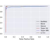
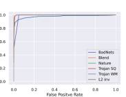
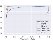
CIFAR10
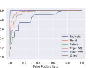
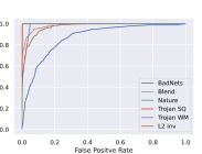
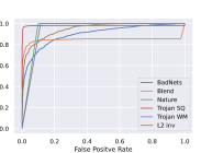
GTSRB
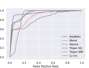
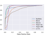
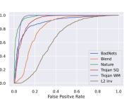
SVHN
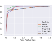
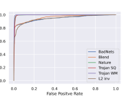
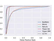
Flower102

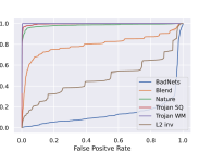
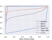
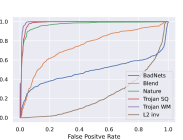
Figure 3. This figure plots ROC curves showing change in accuracy of Trojan sample detection (True positive) with the change in the maximum tolerable false positive rate $\alpha$ for MDTD using FGSM, IFGSM, and HopSkipJump adversarial learning methods for six different types of Trojan triggers- Badnets, Blend, Nature, Trojan SQ, Trojan WM, and L2 inv- for five image-based datasets- CIFAR100, CIFAR10, GTSRB, SVHN, and Flower102. In each case, we observe that the threshold $\alpha$ for the false positive rate plays a critical role in determining values of the true positive rate. Low values of true positive rates despite higher thresholds $\alpha$ when samples in the Flowers102 dataset are embedded with a BadNets (white square) or L2 inv Trojan triggers could be because (uniformly) selected clean input samples in this dataset includes white-colored flowers.

Evaluating MDTD: Table 3 shows the $F_{1}$-scores obtained for images embedded with different types of Trojan triggers when using spectral signature (Tran et al., 2018), activation clustering (Chen et al., 2018), a DCT-based detector (Zeng et al., 2021), STRIP (Gao et al., 2019), and MDTD. Recall from Eqn. (1) that the $F_{1}$-score is defined as $F_{1}=\frac{2*TPR*TNR}{TPR+TNR}$, with $TNR=1-FPR$, where and $TPR$ and $FPR$ denote true and false positive rates.

From Table 3, we observe that MDTD achieves the highest $F_{1}$-scores in almost all cases. This indicates that MDTD is simultaneously able to achieve high true positive rates (detection) and small false positive rates (false alarm). MDTD obtains a lower $F_{1}$-score for only $2$ pairs of cases (Badnets and L2 inv Trojan triggers for Flower102 dataset); we elaborate on these cases in Sec. 7.

Compared to MDTD, SOTA methods that analyze input samples- spectral signature (Tran et al., 2018) and activation clustering (Chen et al., 2018)- have low $F_{1}$-scores due to high false positive rates. DCT-based detectors, on the other hand, show large variations in $F_{1}$-scores across different image-based datasets. Unsurprisingly, DCT-based detectors have very low false positive rates when the number of frequency components in input images is limited (e.g., input samples from SVHN), but they also have very high false positive rates ($\sim 100\%$) when input image samples contain a large number of frequency components (e.g., samples from Flower102). In Appendix B, we report true and false positive rates for each case.

Effect of $\alpha$: Fig. 3 plots ROC curves showing change in the true positive rate with varying values of the maximum tolerable false positive rate threshold $\alpha$ for MDTD using FGSM, IFGSM, and HopSkipJump adversarial learning methods for six different Trojan triggers for all five image-based input datasets. For most datasets, and across Trojan trigger types, MDTD consistently accomplishes high true positive rates for smaller values of $\alpha$.

6.2. Graph Inputs

MDTD (FGSM)	MDTD (IFGSM)

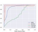
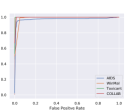
Figure 4. This figure plots ROC curves showing change in accuracy of Trojan sample detection (true positive) with the change in maximum tolerable false positive rate $\alpha$ for MDTD using FGSM and IFGSM adversarial learning methods for four graph-based datasets- AIDS, WinMal, Toxicant, and COLLAB. The threshold $\alpha$ for the false positive rate plays a critical role in determining values of the true positive rate.

AIDS	WinMal	Toxicant	COLLAB

Figure 5. This figure depicts t-SNE visualizations for outputs of the penultimate layer of the GNN model for $200$ clean input graphs (blue dots) and $200$ graph inputs embedded with a Trojan (red dots). We examine four graph-based datasets- AIDS, WinMal, Toxicant, and COLLAB. Similar to our observations for image-based inputs in Fig. 2, we observe that clean and Trojaned samples have different feature values in the penultimate layer.

Datasets: We consider four graph datasets (Xi et al., 2021; Yanardag and Vishwanathan, 2015):

AIDS: This dataset consists $2000$ graphs representing molecular compounds which are constructed from the AIDS Antiviral Screen Database of Active Compounds. The chemical structure of compounds is used to identify whether a patient belongs to one of the following three categories: confirmed active (CA), confirmed moderately active (CM), and confirmed inactive (CI).
WinMal: This dataset consists of $1361$ call graphs of Windows Portable Executable (PE) files. Each file belongs to one of two categories: ‘malware’ or ‘goodware’. Individual nodes of a call graph represent a function and edges between nodes are function calls.
Toxicant: This dataset captures molecular structures (as a graph) of $10000$ compounds studied for their effects of chemical interference in biological pathways. Effects are classified as ‘toxic’ or ‘non-toxic’.
COLLAB: This is a scientific collaboration dataset of $5000$ graphs of ego networks of researchers in 3 fields- High Energy Physics, Condensed Matter Physics, and Astro Physics. The graph classification task is to identify which field an ego network belongs to.

Table 4. This table presents the true positive rate (TPR), False positive rate (FPR), and $F_{1}$-score of MDTD for four graph datasets- AIDS, WinMal, Toxicant, and COLLAB. MDTD (IFGSM) typically achieves a higher $F_{1}$-score (in bold) due to the iterative nature of the IFGSM adversarial learning technique. The $F_{1}$-score for COLLAB is $1$ since MDTD identifies all input samples containing a Trojan trigger correctly ($TPR=1$) and does not raise any false alarm when inspecting clean samples ($FPR=0$).

	MDTD (FGSM)			MDTD (IFGSM)
Task	TPR	FPR	$F_{1}$	TPR	FPR	$F_{1}$
AIDS	$84.07\%$	$14.49\%$	$0.85$	$96.29\%$	$12.88\%$	$\mathbf{0.91}$
WinMal	$96\%$	$10.53\%$	${0.93}$	$100\%$	$7.89\%$	$\mathbf{0.96}$
Toxicant	$25.10\%$	$16.17\%$	$0.39$	$100\%$	$12.77\%$	$\mathbf{0.93}$
COLLAB	$100\%$	$0\%$	$\mathbf{1}$	$100\%$	$0\%$	$\mathbf{1}$

Graph Network Structure: We use identical network structures, parameters, and setups from (Hamilton, 2020) for our experiments, and adopt the Graph Trojan Attack from (Xi et al., 2021) to generate Trojaned GNNs.

Evaluating MDTD: Table 4 shows true positive rate, false positive rate, and $F_{1}$-score for the AIDS, COLLAB, WinMal, and Toxicant datasets. We use MDTD with the FGSM and IFSGM adversarial learning methods to estimate distances of samples to a decision boundary using $100-500$ clean samples (depending on the size of the dataset), and a threshold of $\alpha=0.15$ on the false positive rate. We compute the smallest value $\delta^{*}\in\mathbb{R}^{|V|\times d}$ such that $h(f_{t}(\mathcal{G},X))\neq h(f_{t}(\mathcal{G},X+\delta^{*}))$. As expected, the $F_{1}$-score when using IFGSM is typically higher than when using FGSM due to the iterative nature of the IFGSM adversarial learning technique (Kurakin et al., 2018). For the COLLAB dataset, the $F_{1}$-score is $1$ since MDTD identifies all input samples containing a Trojan trigger correctly ($TPR=1$) and does not raise a false alarm for clean samples ($FPR=0$).

Fig. 4 presents ROC curves showing change in the true positive rate for different values of the maximum tolerable false positive rate threshold $\alpha$ for MDTD using the FGSM and IFGSM adversarial learning methods for the AIDS, COLLAB, WinMal, and Toxicant datasets. Fig. 5 plots representations of feature values of outputs at the penultimate layer of the GNN. We collect $200$ clean graph inputs and 200 graph inputs embedded with a Trojan trigger for the four graph-based input datasets. Our experiments reveal that clean samples (blue dots) can be easily distinguished from Trojan samples (red dots) in all four graph datasets.

Table 5. This Table shows the classification accuracy (Acc.) for clean samples and attack success rate (ASR) for Trojan samples with two different Trojan triggers- Modified (Mod) and Blend (Bld)- on the SpeechCommand dataset. We also report false positive rates (FPR) and $F_{1}$-scores for MDTD (FGSM) and MDTD (IFGSM). We observe that for both triggers, MDTD is able to simultaneously achieve a low FPR and high $F_{1}$-score.

			MDTD (FGSM)		MDTD (IFGSM)
Trojan	Acc.	ASR	FPR	$F_{1}$	FPR	$F_{1}$
Mod	$94.43\%$	$99.95\%$	20.4%	0.81	22.4%	0.80
Bld	$93.31\%$	$99.93\%$	20.4%	0.81	20.4%	0.81

6.3. Audio Inputs

Datasets: We use the SpeechCommand (SC) dataset v.0.02 (Warden, 2018), which contains $65,000$ audio files. Each file is a one-second audio of one of 35 commands. Since some commands are sparse, similar to  (Warden, 5 11) and  (Xu et al., 2021), we select files belonging to ten classes (“yes”, “no”, “up”, “down”, “left”, “right”, “on”, “off”, “stop”, “go”). The dataset for our experiments then has $30,769$ training and $4,074$ test samples.

Network Structure: We trained an LSTM for audio classification on the extracted mel-spectrogram of each file, which contains information about frequency components in the file (Warden, 5 11; Xu et al., 2021).

Evaluating MDTD: Table 5 presents the classification accuracy (Acc.) for clean samples and attack success rate (ASR) for Trojan samples on the SpeechCommand dataset when no defense is used for two types of Trojan triggers- Modified (Mod) and Blend (Bld). We assume that the user has a small set of clean samples ($500$) and estimates a threshold on the distance to a decision boundary with $FPR=15\%$ on this set. We also report false positive rates (FPR) and $F_{1}$-scores for MDTD (FGSM) and MDTD (IFGSM) for $500$ unseen and $500$ Trojan samples. We observe that for both triggers, MDTD is able to simultaneously achieve a low FPR and high $F_{1}$-score.

Fig. 6 shows the t-SNE representations of feature values at the penultimate layer of the LSTM-based DNN. We use $1000$ clean and $1000$ audio samples that have been embedded with a Trojan trigger. We consider two different types of triggers-Modified and Blend- for the SpeechCommand dataset. Our experiments reveal that clean samples (blue dots) can be easily distinguished from Trojan samples (red dots) for both types of triggers.

Modified	Blend

Figure 6. This figure shows t-SNE visualizations for outputs of the penultimate layer of audio LSTM DNN for the SpeechCommand dataset with two different types of Trojan triggers (Modified and Blend) for 1000 clean and 1000 Trojan samples. We observe that for both trigger types, clean and Trojaned samples have different feature values at the penultimate layer.

6.4. MDTD vs. Adaptive Adversary

Table 6. This table reports $F_{1}$-scores of MDTD (IFGSM) for DNN models trained with different levels of adversarial noise ($\epsilon=0.01,\epsilon=0.1$) for the CIFAR10 dataset with six different Trojan triggers. Increasing the value of $\epsilon$ from $0.01$ to $0.1$ results in a reduction of $F_{1}$-score. However, the classification accuracy is reduced, demonstrating a lower utility for an adversary that uses a larger magnitude of adversarial noise perturbation.

$\epsilon$	Attack	Acc.	ASR	$F_{1}$: MDTD (IFGSM)
$0.01$	BadNets	$79.23$	$96.03$	$0.79$
	Blend	$80.19\%$	$99.88\%$	$0.74$
	Nature	$80\%$	$100\%$	$0.93$
	Trojan SQ	$80.06\%$	$100\%$	$0.91$
	Trojan WM	$79.81\%$	$100\%$	$0.90$
	L2 inv	$80.47\%$	$99.98\%$	$0.81$
$0.1$	BadNets	$36.35\%$	$53.74\%$	$0.53$
	Blend	$40.25\%$	$86.88\%$	$0.42$
	Nature	$40.32\%$	$100\%$	$0.85$
	Trojan SQ	$33.62\%$	$100\%$	$0.82$
	Trojan WM	$26.51\%$	$100\%$	$0.68$
	L2 inv	$35.28\%$	$51.90\%$	$0.58$

Table 7. This table reports $F_{1}$-scores of MDTD (IFGSM) for DNN models trained with adversarial noise ($\epsilon=0.01,\epsilon=0.1$) for the AIDS dataset under a Graph Trojan Attack. Increasing the value of $\epsilon$ from $0.01$ to $0.1$ results in a reduction of $F_{1}$-score. However, classification accuracy is reduced, demonstrating a lower utility for an adversary that uses a larger magnitude of adversarial noise perturbation.

$\epsilon$	Acc.	ASR	$F_{1}$: MDTD (IFGSM)
$0.01$	$83\%$	$95.83\%$	$0.96$
$0.1$	$47.77\%$	$92.6\%$	$0.89$

While the threat model presented in Sec. 3 enables consideration of the performance of MDTD with respect to multiple SOTA methods to detect input samples with Trojan-embedded triggers, we now consider a variant of the adversary that is capable of adapting to the two-stage approach of MDTD (Sec. 5.2). Adaptive adversaries have been studied in other contexts, as in (Tramer et al., 2020). Specifically, when the Trojan detection mechanism and hyperparameters of MDTD are known to the attacker, such information can be exploited to carry out an adaptive attack in one of the two following ways.

In the first type of adaptive attack, disrupt MDTD Stage 1, the adversary can add noise to clean samples such that noise-embedded clean samples are adequately distant from the decision boundary. At the same time, Trojan trigger-embedded samples should not be present among noise-perturbed clean samples. Using these modified input samples and Trojan samples, the adversary will need to retrain the DNN model to ensure high classification accuracy of the noise samples, while ensuring that samples embedded with the Trojan trigger are classified to the adversary-desired target class.

If the adversary were then able to deceive the user into adopting this modified Trojaned DNN without the user realizing that the model has been updated, then the user would run only Stage 2 of MDTD (Sec. 5.2) when input samples are provided to the model. This would result in a scenario where a false alarm is raised for clean sample inputs (mislabeled as Trojaned). We carry out experiments to verify this hypothesis and present our results in Table 6 above.

We use the robust learning technique proposed in (Madry et al., 2018). We set the step size to $0.00784$ and examine two noise levels ($\epsilon=0.01,0.1$). Table 6 shows the classification accuracy, ASR, and $F_{1}$-scores for DNN models trained with two levels of adversarial noise perturbations $\epsilon$ for different types of triggers on the CIFAR10 dataset. Increasing $\epsilon$ from $0.01$ to $0.1$ causes a significant drop in the values of $F_{1}$-scores of MDTD. However, this comes at the cost of reducing classification accuracy to below $50\%$. Such low classification accuracy reveals to the user that the DNN model is possibly compromised. The user could then choose to discard the model, rendering the adversary’s efforts futile. Experiments on a nonimage-input graph dataset (AIDS) presented in Table 7 yields similar results.

Table 8. This table reports $F_{1}$-scores of MDTD (IFGSM) for DNN models trained in a way that Trojan samples are assigned their true (correct) label with probability $p$ and assigned the adversary-desired target label otherwise. We report results for $p=0.5,0.7$ for the CIFAR10 dataset with six different Trojan triggers. Increasing the value of $p$ from $0.5$ to $0.7$ results in a marginal change of $F_{1}$-score. However, the $ASR$ value drops significantly, rendering the attack impractical for the adversary.

$p$	Attack	Acc.	ASR	$F_{1}$: MDTD (IFGSM)
$0.5$	BadNets	$80.14\%$	$71.03\%$	$0.16$
	Blend	$80.08\%$	$75.42\%$	$0.80$
	Nature	$79.27\%$	$81.01\%$	$0.88$
	Trojan SQ	$80.48\%$	78.48	$0.89$
	Trojan WM	$79.61\%$	$78.21\%$	$0.93$
	L2 inv	$78.61\%$	$84.63\%$	$0.69$
$0.7$	BadNets	$80.03$	$57.95\%$	$0.12$
	Blend	$79.82\%$	$65.45$%	$0.82$
	Nature	$80.43\%$	$58.28\%$	$0.92$
	Trojan SQ	$75.75\%$	$55.45\%$	$0.91$
	Trojan WM	$79.61\%$	$58.40\%$	$0.91$
	L2 inv	$79.84\%$	$57.67\%$	$0.64$

The second type of adaptive attack uses the insight that DNN models are known to classify Trojan trigger-embedded input samples more confidently (Gao et al., 2019; Qi et al., 2023), which indicates these samples are likely to be further away from a decision boundary (Choquette-Choo et al., 2021). The adversary can thus attempt to disrupt MDTD Stage 1 by moving Trojan samples closer to a decision boundary (Qi et al., 2023). The DNN model is then retrained using the modified Trojan samples and a set of clean samples. We use the technique proposed in (Qi et al., 2023) to reduce the confidence of the DNN in predicting output labels of Trojan samples. An adversary carrying out the adaptive attack in this setting gives the true (correct) label to a Trojan sample with probability $p$ and assigns the (adversary-desired) target label otherwise. We examine two values of $p$ ($=0.5,0.7$), and report our results on the CIFAR10 dataset for six different types of triggers. Table 8 shows that increasing the value of $p$ marginally affects $F_{1}$-scores of MDTD. However, the $ASR$ value drops significantly, rendering such an attack impractical.

On the other hand, the user could decide to run both Stage 1 and Stage 2 of MDTD using a subset of clean samples to recalibrate parameters of MDTD. Once parameters of MDTD are calibrated, as shown in our previous results in this section, MDTD effectively identifies and discards input samples that contain a Trojan trigger. Repeated retraining by the adversary does not help to improve its performance either. Thus, we conclude that MDTD is agnostic to iterative actions of an adaptive adversary.

7. Discussion

Choice of adversarial learning methods: As detailed in Sec. 5.2, in the first stage, MDTD estimates distances of samples to a decision boundary; in the second stage, MDTD applies the described outlier detection procedure to identify input samples that contain a Trojan trigger. The choice of adversarial learning method used to estimate the minimum noise required to change the output of the model could impact the performance of MDTD. For example, in Table 3, in the black-box setting, when using a SOTA adversarial learning method HopSkipJump (Chen et al., 2020), an estimate of such noise is expected to be difficult to obtain. However, MDTD performs quite well even in such a scenario, and obtains high $F_{1}$-scores. Unsurprisingly, in the white-box setting, when MDTD uses computationally inexpensive adversarial learning techniques such as FGSM and IFGSM (Goodfellow et al., 2015), access to model parameters results in even higher $F_{1}$-scores.

$F_{1}$-score of MDTD and robustness of Trojan samples: MDTD obtains a lower $F_{1}$-score in $2$ pairs of cases- observe $F_{1}$-scores in Table 3 for Badnets (white square) or L2 inv Trojan triggers in the Flower102 dataset. ROC curves indicate that true positive rates are lower even when selecting a large threshold $\alpha$ (bottom row of Fig. 3). The Flower102 dataset contains white-colored flowers that are part of clean input samples. On the other hand, as shown in Fig. 1, the Trojan trigger for Badnets is a white square. In this case, overlaying the Badnets trigger on top of a white flower makes it difficult to distinguish between clean samples and samples that contain the trigger. This observation is further reinforced in the last row of Table  1 where clean samples from Flower102 and Trojan samples embedded with the BadNets and L2 inv triggers have comparable values of the average certified radius, but with high variance.

CIFAR100	GTSRB

Figure 7. t-SNE visualizations for outputs of the penultimate layer of the DNN for $200$ clean samples (blue dots) from the target class (Class 6) and $200$ Trojaned samples embedded with a natural backdoor (red dots) misclassified to target class for CIFAR100 (left) and GTSRB (right) datasets. Embedding a Trojan trigger into samples from CIFAR100 is easier than into samples from GTSRB (compare separability of blue and red dots). As a result, input samples from the GTSRB dataset that contain a Trojan trigger will not be effectively classified by the DNN model to the adversary-desired target class. Any detection mechanism, therefore, can be expected to have a high false positive rate, where clean samples are (mistakenly) identified as Trojaned.

Natural Backdoors: Our focus so far has been on embedded backdoor attacks in which an adversary embeds a predefined trigger into inputs given to DNN models. However, an attacker who has knowledge of parameters of the user model, including all decision boundaries, can learn an adversarial noise which can then be used as a natural backdoor (Tao et al., 2022) to ensure that the DNN model output is the adversary-desired label. Such an adversarial noise is also termed a universal perturbation, and it was shown in (Moosavi-Dezfooli et al., 2017) that it was possible for an adversary to learn a universal perturbation and use it to simulate behavior similar to a backdoor attack.

Fig. 7 depicts values in feature space at intermediate layers of DNNs containing natural backdoors for clean input samples and samples containing a Trojan trigger. The t-SNE visualizations for samples from the CIFAR100 (Fig. 7, left) and GTSRB (Fig. 7, right) datasets reveal that embedding a Trojan trigger into samples from CIFAR100 is easier than into samples from GTSRB (compare separability of blue and red dots in Fig. 7). The case of GTSRB shows that use of natural backdoors may not be always effective as Trojan trigger embedding strategy. Consequently, if clean samples and trigger-embedded samples from GTSRB were to mix, then any detection mechanism can be expected to have a high false positive rate.

MDTD for Text Models: Sequence-to-sequence (seq2seq) text models (Sutskever et al., 2014) map an input sequence $x=\{x_{1},.\dots,x_{k}\}$ to an output sequence $y=\{y_{1},\dots,y_{n}\}$, possibly of different length. A backdoor attack on a text model consists of using a specific term or word in the input sequence as the trigger. Similar to Trojaned models for images and graphs, the adversary’s objective is to ensure that the Trojaned text model behaves normally for text inputs that do not contain the trigger word or phrase, and produces an adversary-desired output for inputs that contain the trigger word or phrase. The authors of (Bagdasaryan and Shmatikov, 2022) showed that Trojan triggers could be embedded into seq2seq text models that perform text summarization tasks. The presence of a trigger in the input produced a summarized output that had different properties than desired. For e.g., a trigger in the input text caused the output text to have a different ‘sentiment’ than in the case when the trigger was absent (clean input). A metric that is widely used to determine the quality of text summarization is the ROUGE score (Lin, 2004), which compares the output of a text model with a human-written summary. Although the trigger word in a text summary can be identified by brute-force, such a procedure will be computationally expensive. Further, state-of-the-art in Trojan detection for text models focus on text classification tasks (Sheng et al., 2022).

We believe that MDTD can be used together with ROUGE scores to efficiently detect a trigger word in inputs to text models when a user has access only to a small number of clean inputs. This can be accomplished by using adversarial learning methods to estimate a threshold on the number of words removed that results in the maximum change in ROUGE scores. This remains an open problem.

Black-box Adversarial Learning for DNNs with Graph and Text Inputs: Multiple black-box adversarial learning techniques have been proposed for DNNs with image inputs (Carlini and Wagner, 2017; Moosavi-Dezfooli et al., 2016; Chen et al., 2020). However, black-box adversarial methods for classification tasks on DNN models with text inputs such as those in (Narodytska and Kasiviswanathan, 2017; Gao et al., 2018) are not directly applicable to the other tasks including text summarization. For DNNs with graph inputs, to the best of our knowledge, the only black-box adversarial learning method was presented in (Mu et al., 2021). This approach considered the removal or addition of nodes and edges as a ‘noise’ term, which does not apply to our framework, since we assume that triggers are embedded into feature values of nodes. Suitably modifying SOTA black-box adversarial learning methods such as HopSkipJump (Chen et al., 2020) beyond image-based inputs to use MDTD for Trojan input detection remains a nontrivial open problem.

8. Related Work

We give an overview of defenses against backdoor attacks on DNN models for image and graph inputs.

Images: Defenses against backdoor attacks on DNN models for image-based inputs fall into one of three categories: (i) eliminating the backdoor from the model, (ii) detection mechanisms to identify Trojaned models, and (iii) detecting inputs into which a Trojan has been embedded. Eliminating the backdoor from the DNN model is typically accomplished by pruning the model (Liu et al., 2018a; Aiken et al., 2021) to remove a Trojan trigger or using a small number of samples to retrain the model (Villarreal-Vasquez and Bhargava, 2020). Detection mechanisms to identify Trojaned models involve exhaustively examining a set of models using adversarial learning (Goodfellow et al., 2015) to reverse engineer a trigger, e.g., Neural Cleanse (Wang et al., 2019). The authors of (Shen et al., 2021) proposed an optimization strategy to overcome the challenge of exhaustively examining the set of DNN models. A GAN-based method to synthesize Trojan triggers was proposed in (Zhu et al., 2020), which reduced the number of samples required in order to detect the trigger. Methods to detect input samples into which a Trojan trigger has been embedded filter out suspicious samples at training or inference time. The authors of (Tran et al., 2018) proposed spectral signature method which uses singular value decomposition of a covariance matrix associated to sample representations to compute an outlier score. Similar to spectral signature, activation clustering (Chen et al., 2018) aims to detect Trojan samples by analyzing neural network activations. Unlike MDTD, spectral signature and activation clustering methods are designed for training phase and their goal is to eliminate Trojan samples from the training set. However, they may mistakenly eliminate clean samples, which limits their usability as a Trojan sample detection mechanism in the inference phase. A technique called STRIP was proposed in (Gao et al., 2019), where DNN outputs were used to distinguish clean from Trojan samples. A DCT-based detector in (Zeng et al., 2021) used frequency analysis to distinguish between clean and Trojan samples. The above methods are either computationally expensive, as shown in (Li et al., 2022) or are restricted to image-based inputs. In comparison, MDTD requires limited computational resources and is applicable to a wide variety of input domains.

Graphs: Defenses against backdoor attacks on GNNs have been less explored. A smoothed classifier was used in (Zhang et al., 2021) to generate multiple subgraphs by sampling a subset of vertices and edges from the original GNN. A majority-based rule was then used to determine the label associated to each subgraph. An preprocessing step was used to identify nodes of the graph into which an adversary had embedded a Trojan trigger in (Wu et al., 2019). This work used the insight that the presence of an edge between two ‘dissimilar’ nodes was an indication that one of the nodes was Trojaned. Different from these works, MDTD updates features associated to nodes in a GNN whenever nodes and edges of a Trojaned subgraph are altered. One other approach to determine whether a GNN has been Trojaned or not is through the use of an explainability score (Jiang and Li, 2022). This method uses a small set of clean samples to determine a threshold explanability score; an input to the GNN is then classified as Trojan if its explainability score is greater than this threshold.

9. Conclusion

In this paper, we developed a multi-domain Trojan detector (MDTD), which was designed to detect Trojan trigger-embedded input samples in image, graph, and audio-based datasets at testing time. MDTD leveraged an insight that samples containing a trigger were typically located farther away from a decision boundary compared to a clean sample to determine whether a given sample contained a trigger. Qualitatively, we demonstrated this insight by showing that t-SNE visualizations revealed different values of features corresponding to clean and Trojaned samples. Quantitatively, we used adversarial learning techniques to estimate the distance of samples to a decision boundary to infer whether the sample was Trojaned or not. We evaluated MDTD against four state-of-the-art Trojan detection methods on five widely used image datasets- CIFAR100, CIFAR10, GSTRB, SVHN, and Flower102. We also evaluated MDTD on four graph-based datasets- AIDS, WinMal, Toxicant, and COLLAB, and one audio dataset SpeechCommand. In all cases, MDTD effectively identified input samples containing different types of Trojan triggers. We further evaluated MDTD against an adaptive adversary that trains a robust model to increase distance of samples to a decision boundary. In this case, we showed that a reduction in the detection rate of MDTD below $60\%$ is accompanied by a severe reduction in the clean sample classification accuracy of the Trojaned DNN (to $<50\%$), making the model unfit for use.

Appendix

Table 9. This table shows the true positive/ false positive rates for spectral signature (Tran et al., 2018), activation clustering (Chen et al., 2018), DCT-based detectors (Zeng et al., 2021), STRIP (Gao et al., 2019), and MDTD (ours) for six different Trojan triggers for five image datasets. Lower values of $F_{1}$-scores for spectral signature, activation clustering, STRIP, and DCT-based detection observed in Table 3 in the main paper are a consequence of higher values of false positive rates. Higher $F_{1}$-scores for DCT-based detection in Table 3 in some cases is due to large true positive rates combined with low false positive rates. However, DCT-based detectors require access to the entire training set, which makes the process computationally expensive. In comparison, MDTD (noted by bold columns) is able to accomplish high true positive and low false positive rates by using only a small set of labeled clean samples (need not belong to the training set).

	Attack	Spec	AC	DCT-based	STRIP	MDTD (FGSM)	MDTD (IFGSM)	MDTD (HopSkipJump)
CIFAR100	Badnets	$75.73/74.27$	$4.76/18.28$	$87.23/11.58$	$95.80/8.20$	$95.2/4.4$	$92.8/4$	$77.6/3.6$
	Blend	$75.46/74.54$	$0.01/38.88$	$99.53/11.58$	$99.4/9.1$	$99.6/4.6$	$100/3.60$	$99.8/6.6$
	Nature	$75.25/74.75$	$31.20/19.81$	$99.62/11.58$	$100/8.7$	$100/3.6$	$100/4.4$	$100/3$
	Trojan SQ	$75.73/74.27$	$27.47/16.48$	$99.62/11.58$	$100/8.30$	$100/4.8$	$100/6$	$100/6.6$
	Trojan WM	$75.75/74.25$	$42.01/19.05$	${100}/11.58$	$100/9.3$	$100/6.8$	$100/3.2$	$70.8/7$
	L2 inv	$75.60/74.40$	$0.01/36.50$	${100}/11.58$	$99.5/9.8$	$100/3.8$	$99.9/5.8$	$97.8/3.8$
CIFAR10	Badnets	$79.06/70.94$	$100.00/87.43$	$95.20/44.92$	$93/28.3$	$69.9/11.4$	$70.90/16.60$	$80.6/17$
	Blend	$79.04/70.96$	$100/82.40$	${97.71}/44.92$	$98/27.2$	$97.2/12.8$	$97.2/13.6$	$84.50/15.6$
	Nature	$78.60/71.40$	$100/88.60$	$99.91/44.92$	$96.3/29.8$	$100/11$	$100/14$	$100/16.4$
	Trojan SQ	$78.80/71.20$	$100/82.90$	$99.87/44.92$	$99.1/27.8$	$100/16.4$	$100/13$	$98.10/17$
	Trojan WM	$78.88/71.12$	$0.03/44.10$	$99.87/44.92$	$99.9/28.9$	$100/16.2$	$100/17$	$100/13.60$
	L2 inv	$78.89/71.11$	$100/76.70$	${99.99}/44.92$	$98.5/26.4$	$90.7/8.8$	$95.4/13.8$	$88.4/17.4$
GTSRB	Badnets	$75.89/74.01$	$100/89.97$	$77.31/{9.08}$	$95.8/32.2$	$91.70/15.8$	$88.5/8.8$	$84.9/2$
	Blend	$75.89/74.01$	$100/98.69$	$58.95/9.08$	$94.1/39$	$91.9/36.2$	$78.9/13.4$	$91.50/34.4$
	Nature	$75.89/74.01$	$100/99.05$	$78.24/{9.08}$	$99.8/38.6$	$100/38.6$	$100/18.2$	$100/38.6$
	Trojan SQ	$74.81/75.09$	$100/94.92$	$98.58/9.08$	$97/33.1$	$99.6/32.6$	$98.4/18.8$	$99.2/34.2$
	Trojan WM	$75.71/74.20$	$100/99.05$	$99.21/{9.08}$	$96.4/37$	$100/22.6$	$100/15.6$	$100/16.2$
	L2 inv	$75.84/74.06$	$100/92.07$	$95.25/9.08$	$84.9/34.2$	$65.3/24.6$	$66.1/15.4$	$6.7/12.40$
SVHN	Badnets	$80.56/69.44$	$100/74.70$	$99.96/0.21$	$86.20/12.60$	$90.8/28.8$	$88.60/13.6$	$80.9/17.4$
	Blend	$80.70/69.30$	$18.20/45.52$	$99.97/0.21$	$98.8/38.3$	$90.70/34.60$	$88.8/10.2$	$88.80/22.2$
	Nature	$80.70/69.30$	$4.82/7.59$	$99.97/{0.21}$	$99.7/38.7$	$99.90/36.60$	$99.9/10.6$	$100/30.4$
	Trojan SQ	$80.70/69.30$	$6.89/7.59$	$99.97/{0.21}$	$99.4/41.2$	$100/45.2$	$100/16$	$99.9/30$
	Trojan WM	$80.67/69.32$	$5.21/7.47$	$99.97/{0.21}$	$99.60/38.7$	$100/29.40$	$100/13.80$	$100/20.6$
	L2 inv	$80.65/69.35$	$23.29/46.93$	$99.97/{0.21}$	$67.5/41.6$	$89/15.4$	$90.70/17.4$	$100/16.4$
Flower102	Badnets	$74.80/70.20$	$100/88.04$	$99.98/100$	$31.8/1.2$	$4.7/17$	$4.40/13.2$	$35.10/13.2$
	Blend	$74.71/70.29$	$100/84.51$	${100}/100$	$28.7/0.6$	$73/16.6$	$82.60/15$	$51.2/12.20$
	Nature	$74.71/70.29$	$100/19.22$	${100}/100$	$29/0.40$	$97.50/18$	$99.30/13.2$	$95.90/14.4$
	Trojan SQ	$74.71/70.29$	$100/85.69$	${100}/100$	$78.8/0.4$	$99.5/12.8$	$100/14.20$	$99.50/14.60$
	Trojan WM	$74.71/70.29$	$100/84.12$	$100/100$	$60.1/0.5$	$100/15.6$	$100/14.2$	$100/15$
	L2 inv	$74.80/70.20$	$100/87.84$	${100}/100$	$66/1$	$25.5/11.2$	$58.9/13$	$1.3/18.2$

Appendix A: Worst-Case False Positive Rate

This Appendix presents a theoretical characterization of the worst-case false positive rate of MDTD.

Theorem: Assume that the function $f$ in Eqn. (2) is differentiable, and that its gradient $\nabla_{x}f$ is locally Lipschitz. For any clean sample $x$, the worst-case false positive rate of MDTD is given by

(5) $$\mathbb{P}(\text{MDTD identifies }x\text{ as Trojan})\leq e^{-(\zeta+\alpha\sigma)^{2}/2\sigma^{2}},$$

where $\zeta=\frac{L\|\nabla_{f}\mathcal{L}\|\|x-\hat{x}\|}{2\lambda-L\|\nabla_{f}\mathcal{L}\|}$, and $\hat{x}=\operatorname*{argmin}_{x^{\prime}\in D_{user}}\|x^{\prime}-x\|_{1}$ is the sample from $D_{user}$ that belongs to the same class as $x$.

Proof:  We first quantify the range of values of the distance of a clean sample $x$ to a decision boundary in terms of its certified radius $\delta$. We then use these range of values to determine the worst-case false positive rate of MDTD.

Let $\hat{x}=\operatorname*{argmin}_{x^{\prime}\in D_{user}}\|x^{\prime}-x\|_{1}$ and $\hat{\delta}$ be the certified radius of $\hat{x}$. Since $f$ is differentiable, $\delta$ and $\hat{\delta}$ must be critical points of:

$$-\nabla_{f}\mathcal{L}\nabla_{x}f|_{x+\delta}+2\lambda\delta=0;-\nabla_{f}\mathcal{L}\nabla_{x}f|_{\hat{x}+\hat{\delta}}+2\lambda\hat{\delta}=0,$$

respectively. We thus have that

(6a) $$~{}\|2\lambda\delta-2\lambda\hat{\delta}\|_{1}=\|\nabla_{f}\mathcal{L}\nabla_{x}f|_{x+\delta}-\nabla_{f}\mathcal{L}\nabla_{x}f|_{\hat{x}+\hat{\delta}}\|_{1}$$

(6b) $$\leq ~{}\|\nabla_{f}\mathcal{L}\|_{1}L\|\hat{x}-x+\hat{\delta}-\delta\|_{1}$$

(6c) $$\leq ~{}\|\nabla_{f}\mathcal{L}\|_{1}L(\|\hat{x}-x\|_{1}+\|\hat{\delta}-\delta\|_{1})$$

where inequalities Equation (6b) and Equation (6c) hold by the assumption that $\nabla_{x}f$ is locally Lipschitz and the triangle inequality, respectively. Rearranging Equation (6) yields

(7) $$\|\delta-\hat{\delta}\|_{1}\leq\frac{L\|\nabla_{f}\mathcal{L}\|_{1}\|x-\hat{x}\|_{1}}{2\lambda-L\|\nabla_{f}\mathcal{L}\|_{1}}\triangleq\zeta.$$

Given parameters $\mu$ and $\sigma$ which are estimated using the clean data set $D_{user}$, we can quantify the worst-case false positive rate for clean sample $x$ as

(8) $$\mathbb{P}(\text{MDTD identifies }x\text{ as Trojan})= ~{}\mathbb{P}(|\delta-\mu|\geq\alpha\sigma)$$

(9) $$\leq ~{}\mathbb{P}(|\hat{\delta}-\zeta-\mu|\geq\alpha\sigma).$$

Eqn. (9) follows from Eqn. (7) and the fact that we focus on the upper tail of the Gaussian distribution. Using the tail bound of Normal distribution (Mitzenmacher and Upfal, 2017), we have $\mathbb{P}(|\hat{\delta}-\zeta-\mu|\geq\alpha\sigma)\leq e^{-(\zeta+\alpha\sigma)^{2}/2\sigma^{2}}$.

Appendix B: True and False Positive Rates for Trojan Triggers on Image Datasets

In Sec. 5, Table 3 presented $F_{1}$ scores for spectral signature (Tran et al., 2018), activation clustering (Chen et al., 2018), DCT-based detectors (Zeng et al., 2021), STRIP (Gao et al., 2019), and MDTD for six different Trojan triggers for five image datasets- CIFAR100, CIFAR10, GTSRB, SVHN, and Flowers102. Table 9 presents values of true and false positive rates for spectral signature (Tran et al., 2018), activation clustering (Chen et al., 2018), DCT-based detectors (Zeng et al., 2021), STRIP (Gao et al., 2019), and MDTD for six different Trojan triggers for the same five datasets.

We examine variants of MDTD when a user has white-box access (MDTD (FGSM) and MDTD (IFGSM)) and black-box access (MDTD (HopSkipJump)) to the DNN model. We observe that DCT-based detectors are able to simultaneously achieve high TPR and low FPR for the SVHN and Flowers102 datasets. However, the DCT-based detector method requires access to the entire training dataset, which makes it computationally expensive. On the other hand, MDTD is able to simultaneously achieve high true positive and low false positive rates even when a user has access to only a small set of labeled clean samples that need not be a part of the training set.

Appendix C: Adaptive Adversary for Audio

In this appendix, we evaluate MDTD against an adversary seeking to disrupt MDTD Stage 1 by adding noise to clean samples for nonimage audio-based inputs such that noise-embedded clean samples are adequately distant from the decision boundary.

Table 10 shows $F_{1}$-scores of MDTD (IFGSM) for DNNs trained without adversarial noise ($\epsilon=0.000$) vs. with adversarial noise ($\epsilon=0.001$) for the SpeechCommand audio dataset with two different Trojan triggers- Modified (Mod) and Blend (Bld). Increasing the value of $\epsilon$ results in a reduction of $F_{1}$-score for the Mod trigger. This indicates that an adaptive adversary is more effective in reducing effectiveness of MDTD for audio inputs with a Mod trigger than when using a Bld trigger. However, different from our results for image (Table 6) and graph (Table 7) inputs, classification accuracy is only marginally affected. We provide a possible explanation below.

Each audio sample in the SpeechCommand dataset can be of a different length or time-duration, and different samples can belong to widely different ranges of values. This is unlike for images, where each pixel takes a value in a known interval- e.g., $[0,1]$ for black-white and $[0,255]$ for color images. Such large variations in length and value make training of robust DNNs challenging, since adding (small amounts of) adversarial noise can result in minimal impact on sample values, and consequently, on classification accuracy.

Table 10. This table reports $F_{1}$-scores of MDTD (IFGSM) for DNN models trained without adversarial noise ($\epsilon=0.000$) vs. with adversarial noise ($\epsilon=0.001$) for the SpeechCommand audio dataset with two different Trojan triggers. Increasing the value of $\epsilon$ results in a reduction of $F_{1}$-score for the Mod trigger. However, classification accuracy is only marginally affected, indicating that an adaptive adversary is more effective in reducing effectiveness of MDTD for audio inputs than for image inputs without sacrificing classification accuracy (compare with results in Tables 6. 7).

$\epsilon$	Attack	Acc.	ASR	$F_{1}$: MDTD (IFGSM)
$0.000$	Mod	$94.43$	$99.95$	$0.80$
	Bld	$93.31\%$	$99.93\%$	$0.81$
$0.001$	Mod	$94.65\%$	$99.75\%$	$0.69$
	Bld	$94.25\%$	$94.97\%$	$0.82$