Asymptotics for Short Maturity Asian Options in a Jump-Diffusion model with Local Volatility

Abstract.

We present a study of the short maturity asymptotics for Asian options in a jump-diffusion model with a local volatility component, where the jumps are modeled as a compound Poisson process which are later extended to Lévy jumps, that includes the exponential Lévy model as a special case. Both fixed and floating strike Asian options are considered. Explicit results are obtained for the first-order asymptotics of the Asian options prices for a few popular models in the literature: the Merton jump-diffusion model, the double-exponential jump model, and the Variance Gamma model. We propose an analytical approximation for Asian option prices which satisfies the constraints from the short-maturity asymptotics, and test it against Monte Carlo simulations. The asymptotic results are in good agreement with numerical simulations for sufficiently small maturity.

1. Introduction

Asian options are popular instruments traded in many financial markets, on underlyings such as commodity futures, equities, indices and currency exchange rates (FX). Compared to vanilla European options they have the advantage that they are less sensitive to short term price fluctuations of the underlying asset, due to their averaging property. Typically, such options have a payoff of the form:

(1) $$\mbox{Payoff}=\left(\theta(A_{T}-K),0\right)^{+}\,,$$

where $A_{T}$ is the average of the asset price $S_{t}$ over an averaging period $[T_{1},T_{2}]$, and $\theta=\pm 1$ for a call/put Asian option. Although in practice the averaging is in discrete time (daily averaging), it is convenient to approximate $A_{T}$ with the continuous time average:

(2) $$A_{T}:=\frac{1}{T_{2}-T_{1}}\int_{T_{1}}^{T_{2}}S_{t}dt\,.$$

Most of the theoretical work on pricing Asian options assumes that the asset price follows a diffusion process, with continuous sample paths. We summarize briefly a few results using methods which can be extended to models with jumps.

Geman and Yor [28] found an exact result for the price of an Asian option in the Black-Scholes model with random maturity $T_{\lambda}\sim\text{Exp}(\lambda)$, distributed according to an exponential distribution with parameter $\lambda$. This reduces the pricing of such options to the inversion of a Laplace transform. See [16, 20, 25] for details of application of this method.

A generalization of this approach was proposed by Cai and Kou [10] who showed that the double Laplace transform of the Asian option prices with respect to strike and maturity has a very simple form and can be computed exactly in a wide class of models. This reduces the Asian options pricing problem to the inversion of a double Laplace transform, for which efficient numerical methods are available. This method was applied in [30] to models driven by hyper-exponential Lévy processes, which are generalizations of models with hyper-exponential jumps.

The Cai, Kou approach has been simplified by Cai, Song and Kou [12] by approximating the underlying process for $S_{t}$ with a finite state Markov chain. The double Laplace transform of the Asian price with respect to strike and maturity can be expressed as a matrix multiplication. This method has been simplified further in [13] by performing one Laplace inversion analytically, which reduces the problem to the inversion of a single Laplace transform.

Another approach proposed is the PDE method [44, 47, 48]. The Asian option pricing PDE can be solved either numerically, or using asymptotic expansion methods. We note the paper of [24] which applied this method to derive precise expansions for Asian option prices in the local volatility model. Another very flexible method which can be used for models where $\log S_{t}$ has independent increments is a backward recursion combined with Fourier inversion methods. This was first proposed for the Black-Scholes (BS) model by Carverhill and Clewlow [14], and improved by Benhamou [8]. The method was later extended to exponential Lévy models by Fusai [26] and Fusai, Meucci [27]. An alternative recursion method has been presented in [41] for pricing discrete sampled Asian options in the BS model.

In [40] the authors obtained an asymptotic expansion for Asian options prices in the short-maturity limit $T\to 0$ in the local volatility model. Using large deviations theory methods [19, 46], asymptotics for out-of-the money Asian options have been derived. For a general local volatility model the short maturity asymptotics is expressed in terms of a rate function which is given in terms of quadratures. The result can be put in explicit form for the CEV model [42]. The at-the-money (ATM) asymptotics has been obtained as well, which is dominated by the fluctuations of the asset price around the spot price. We mention also the results of Gobet and Miri [29] who studied the expansion of the time-average of a diffusion in a small parameter such as time or volatility using Malliavin calculus, with applications to pricing Asian options. The implied volatility of Asian options in stochastic volatility models was studied recently in Alòs et al. [2] in a region of strikes close to the ATM point. Also, Cai et al. [11] presented closed-form expansions for Asian options with discrete time averaging in diffusion models.

One important question is the impact of jumps on the pricing of Asian options. It is intuitively clear that jumps can have an important effect on the price of an out-of-the-money (OTM) Asian options with small maturity, as the jump could possibly take the option into in-the-money. Evidence for discontinuous behavior in the dynamics of many financial assets has been presented in [17]. Since the economic motivation for trading Asian options is to smooth out the impact of short term price fluctuations, it is important to have a quantitative understanding of the jumps impact.

The simplest jump-diffusion model is the Merton model [37], where the log-asset price $\log S_{t}$ is the sum of a standard Brownian motion plus a compound Poisson process with constant intensity $\lambda$ and normally distributed jump size. The pricing of Asian options on commodity futures including stochastic volatility and jumps distributed according to the Merton model has been presented in [34].

The impact of adding exactly one jump to the Black-Scholes model on the pricing of Asian options has been studied in [18]. Another popular model is the double-exponential jump model of Kou [32], where the jump sizes can be both positive and negative, and are exponentially distributed. American option pricing under this model has been studied in [33], and pricing of Asian options has been presented in [10].

The model of [32] has been generalized to the hyper-exponential model (HEM) where the jump size distribution is a linear superposition of exponential distributions with the density:

(3) $$f_{Y}(x)=\sum_{i=1}^{n}p_{i}\eta_{i}e^{-\eta_{i}x}1_{x\geq 0}+\sum_{j=1}^{n}q_{j}\theta_{j}e^{\theta_{j}x}1_{x<0}\,.$$

This model is widely used in the mathematical finance literature, and has been used for pricing options and exotic derivatives, such as barrier and American-type options by Boyarchenko and Levendorskii [9] and Cai and Kou [10] for Asian options. By Bernstein’s theorem the hyper-exponential distribution can approximate any Lévy process with completely monotone density $\nu(dx)$. Lévy processes commonly used in finance for the CGMY, NIG and VG models are completely monotone.

We comment also on the PDE method, which can be applied also in the presence of jumps [47, 48], when the PDE becomes an integro-differential equation. The smoothness properties of the solution of this equation are not trivial, and they have been studied in [6].

We will study in this paper the impact of jumps on the short-maturity asymptotics of Asian options. In contrast to the European options which have been considered in the literature in the regime of small maturity, the case of the Asian options has been less well studied. The short-maturity asymptotics for European call and put options has been studied in the literature, under exponential Lévy models and jump-diffusion models.

We summarize here a few results for the exponential Lévy models, and we refer to [22] for a more detailed list of references. See also [1] for work on short-maturity expansions in jump-diffusion models using Malliavin calculus methods. Consider an exponential Lévy model $S_{t}=S_{0}e^{X_{t}}$ where $X_{t}$ is a Lévy process with density $\nu(dx)$ that starts at $0$ at time zero. In a wide class of such models, the leading short-maturity asymptotics of the European call options is given by [9]:

(4) $$\lim_{T\to 0}\frac{1}{S_{0}T}\mathbb{E}[(S_{T}-K)^{+}]=\int(e^{x}-(K/S_{0}))^{+}\nu(dx)\,,\qquad K>S_{0}\,.$$

A sufficient condition for this result to hold is $\int\min(|x|^{2},1)e^{x}\nu(dx)<\infty$. See [21] for weaker conditions. The next-to-leading order correction of $O(T^{2})$ to the short-maturity asymptotics has been obtained in [22], and the leading asymptotics of the ATM skew was studied in [23].

In this paper we consider the pricing of Asian options in a wide class of jump-diffusion models where the diffusion is given by a local volatility model, and the jumps are modeled as compound Poisson processes (Section 2). This generalizes the Merton and Kou models by allowing for a more general diffusion process. We consider the generalization to a general exponential Lévy process in Section 3. Asymptotics for floating strike Asian options will be discussed in Section 4. Explicit asymptotic results are given for the Asian options prices in the short maturity limit for some of the most popular models with jumps in the literature: the Merton jump-diffusion model, the double-exponential jump diffusion model, and the Variance Gamma model (Section 5). The asymptotic results are compared with independent MC simulations of Asian options in these models in Section 6.

2. Main Results

Let $S_{t}$ be the asset price process. Assume that $r$ is the risk-free rate and $q$ is the dividend yield. We are interested in the short-maturity limit as the maturity $T\rightarrow 0$. In Pirjol and Zhu [40], the asset price is assumed to follow a local volatility model:

(5) $$\frac{dS_{t}}{S_{t-}}=(r-q)dt+\sigma(S_{t})dW_{t},\qquad S_{0}>0.$$

We assume that the local volatility function $\sigma(\cdot)$ satisfies

(6) $$0<\underline{\sigma}\leq\sigma(\cdot)\leq\overline{\sigma}<\infty,$$

(7) $$|\sigma(e^{x})-\sigma(e^{y})|\leq M|x-y|^{\alpha},$$

for some fixed $M,\alpha>0$ for any $x,y$ and $0<\underline{\sigma}<\overline{\sigma}<\infty$ are some fixed constants. This is the same assumption used in Pirjol and Zhu [40] to obtain the short maturity asymptotics for Asian options in local volatility models. This assumption originally came from the paper of Varadhan [45] for short time interval diffusion processes.

In this paper, we add the compound Poisson jumps independent of the diffusion part (and later we will extend our results to allow Lévy jumps in Section 3), that is,

(8) $$S_{t}=\hat{S}_{t}e^{\sum_{i=1}^{N_{t}}Y_{i}},$$

where $\hat{S}_{t}$ follows a local volatility model:

(9) $$\frac{d\hat{S}_{t}}{\hat{S}_{t-}}=(r-q)dt-\lambda\mu dt+\sigma(\hat{S}_{t})dW_{t},\qquad\hat{S}_{0}=S_{0},$$

where $\sum_{i=1}^{N_{t}}Y_{i}$ is a compound Poisson process independent of $\hat{S}$ process, and $\mu=\mathbb{E}[e^{Y_{1}}-1]$, and the jumps $Y_{i}$ are i.i.d. with the probability distribution function $P(y)$, $-\infty<y<\infty$, that is, we allow both positive and negative jumps and $Y_{i}$’s are independent of the Poisson process $N_{t}$ with an intensity $\lambda>0$.

Extensions of the local volatility model by adding jumps have been considered in the literature by Andersen and Andreasen [4], Benhamou, Gobet, Miri [7] and Pagliarani and Pascucci [39].

We will make the following assumption about the jump size distribution in the compound Poisson process:

Assumption 1.

The jumps $Y_{1}$ satisfy the condition

(10) $$\mathbb{E}[e^{\theta Y_{1}}]<\infty,\qquad\text{for some $\theta>2$}.$$

The price process $S_{t}$ can be written alternatively as

(11) $$S_{t}=S_{0}e^{\int_{0}^{t}\sigma(\hat{S}_{s})dW_{s}+(r-q-\lambda\mu)t-\int_{0}^{t}\frac{1}{2}\sigma^{2}(\hat{S}_{s})ds+\sum_{i=1}^{N_{t}}Y_{i}}.$$

As the maturity $T\rightarrow 0$, we have $S_{T}\rightarrow S_{0}$ a.s. We are interested in the asymptotics of the out-of-the money Asian call option price:

(12) $$C(T)=e^{-rT}\mathbb{E}\left[\left(\frac{1}{T}\int_{0}^{T}S_{t}dt-K\right)^{+}\right].$$

The $T\to 0$ asymptotics of out-of-the-money Asian call options in the model where $S_{t}$ follows a local volatility model without jumps was studied in Pirjol and Zhu [40] and it is of the order $e^{-O(\frac{1}{T})}$. Similar results were obtained in [5]. In the presence of jumps, the leading order will change. The intuition behind this is that the probability of one jump is of the order $O(T)$, and one single jump can make the asset price process back to the in-the-money region. Since the probability of getting into the in-the-money region from the contributions of the diffusions is of the order $e^{-O(\frac{1}{T})}$, it is intuitively clear that in the presence of jumps, $C(T)=O(T)$. So the key question here is to determine the precise leading order asymptotics for $C(T)$ as the maturity $T\rightarrow 0$.

We have the following main result:

Theorem 2.

Assume that the asset price $S_{t}$ follows the process (8) and the jump distribution satisfies Assumption 1. Then the leading order asymptotics for out-of-the-money, i.e. $K>S_{0}$, short maturity Asian call options is given by

(13) $$\lim_{T\rightarrow 0}\frac{C(T)}{T}=\lambda\int_{0}^{1}\int_{\log(\frac{K-S_{0}t}{S_{0}(1-t)})}^{\infty}\left(S_{0}t+S_{0}e^{y}(1-t)-K\right)dP(y)dt,$$

provided that the limit is positive.

Proof.

Note that

(14) $$C(T) =e^{-rT}\mathbb{E}\left[\left(\frac{1}{T}\int_{0}^{T}S_{t}dt-K\right)^{+}1_{N_{T}=0}\right]+e^{-rT}\mathbb{E}\left[\left(\frac{1}{T}\int_{0}^{T}S_{t}dt-K\right)^{+}1_{N_{T}=1}\right]$$

$$\qquad+e^{-rT}\mathbb{E}\left[\left(\frac{1}{T}\int_{0}^{T}S_{t}dt-K\right)^{+}1_{N_{T}\geq 2}\right].$$

Next, let us analyze each of the three terms in (14) carefully.

Let us first consider the first term in (14). The probability that there is no Poisson jump is given by $\mathbb{P}(N_{T}=0)=e^{-\lambda T}$. Conditional on zero jumps on the interval $[0,T]$, $S_{t}=\hat{S}_{t}$ process satisfies the local volatility model:

(15) $$\hat{S}_{t}=S_{0}e^{\int_{0}^{t}\sigma(\hat{S}_{s})dW_{s}+(r-q-\lambda\mu)t-\int_{0}^{t}\frac{1}{2}\sigma^{2}(\hat{S}_{s})ds}.$$

By using the OTM Asian call option result from Pirjol and Zhu [40], we get

(16) $$e^{-rT}\mathbb{E}\left[\left(\frac{1}{T}\int_{0}^{T}S_{t}dt-K\right)^{+}1_{N_{T}=0}\right] =e^{-rT}e^{-\lambda T}\mathbb{E}\left[\left(\frac{1}{T}\int_{0}^{T}\hat{S}_{t}dt-K\right)^{+}\right]$$

$$=e^{-rT}e^{-\lambda T}e^{-\mathcal{I}(K,S_{0})\frac{1}{T}+o(\frac{1}{T})},$$

as $T\rightarrow\infty$.

Next, let us consider the third term in (14). By Hölder’s inequality, for any $\frac{1}{p}+\frac{1}{p^{\prime}}=1$, where $p,p^{\prime}>1$, we have

(17) $$e^{-rT}\mathbb{E}\left[\left(\frac{1}{T}\int_{0}^{T}S_{t}dt-K\right)^{+}1_{N_{T}\geq 2}\right]$$

$$\leq e^{-rT}\mathbb{E}\left[\left(\frac{1}{T}\int_{0}^{T}S_{t}dt\right)1_{N_{T}\geq 2}\right]+e^{-rT}\mathbb{E}\left[K1_{N_{T}\geq 2}\right]$$

$$\leq e^{-rT}\left(\mathbb{E}\left[\left(\frac{1}{T}\int_{0}^{T}S_{t}dt\right)^{p}\right]\right)^{1/p}\left(\mathbb{E}[(1_{N_{T}\geq 2})^{p^{\prime}}]\right)^{1/p^{\prime}}+e^{-rT}K\mathbb{P}(N_{T}\geq 2)$$

$$\leq e^{-rT}C\cdot O(T^{2/p^{\prime}})+e^{-rT}K\cdot O(T^{2}).$$

Let us choose $1<p^{\prime}<2$, which is ensured by taking $p$ to be some value greater than $2$, which is made possible by Assumption 1. Then, the third term in (14) is bounded above by $O(T^{2/p^{\prime}})$, with $2/p^{\prime}>1$. Thus we proved that the third term in (14) is $o(T)$.

We give next the proof of the estimate in the last line of equation (17). First, note that $\mathbb{P}(N_{T}\geq 2)=1-e^{-\lambda T}-\lambda Te^{-\lambda T}=O(T^{2})$ as $T\rightarrow 0$. Moreover, note that $\frac{S_{t}}{e^{(r-q)t}}=:M_{t}$ is a positive martingale. Therefore by the Doob’s martingale inequality,

(18) $$\left(\mathbb{E}\left[\left(\frac{1}{T}\int_{0}^{T}S_{t}dt\right)^{p}\right]\right)^{1/p} \leq\left(\mathbb{E}\left[\max_{0\leq t\leq T}S_{t}^{p}\right]\right)^{1/p}$$

$$\leq e^{|r-q|T}\left(\mathbb{E}\left[\max_{0\leq t\leq T}M_{t}^{p}\right]\right)^{1/p}$$

$$\leq e^{|r-q|T}C_{p}\left(\mathbb{E}\left[M_{T}^{p}\right]\right)^{1/p}\,,$$

with $C_{p}=\frac{p}{p-1}$. Furthermore, we have

$$\left(\mathbb{E}\left[M_{T}^{p}\right]\right)^{1/p} =e^{-(r-q)T}\left(\mathbb{E}\left[S_{T}^{p}\right]\right)^{1/p}$$

$$=e^{-(r-q)T}\left(\mathbb{E}\left[S_{0}^{p}e^{p\int_{0}^{T}\sigma(\hat{S}_{s})dW_{s}+p(r-q-\lambda\mu)T-p\int_{0}^{T}\frac{1}{2}\sigma^{2}(\hat{S}_{s})ds+p\sum_{i=1}^{N_{T}}Y_{i}}\right]\right)^{1/p}$$

$$=e^{-(r-q)T}S_{0}e^{(r-q-\lambda\mu)T}$$

$$\qquad\cdot\left(\mathbb{E}\left[S_{0}^{p}e^{p\int_{0}^{T}\sigma(\hat{S}_{s})dW_{s}-\frac{\alpha}{2}p^{2}\int_{0}^{T}\sigma^{2}(\hat{S}_{s})ds+(\frac{\alpha}{2}p^{2}-\frac{1}{2}p)\int_{0}^{T}\sigma^{2}(\hat{S}_{s})ds+p\sum_{i=1}^{N_{T}}Y_{i}}\right]\right)^{1/p}$$

$$\leq e^{-(r-q)T}S_{0}e^{(r-q-\lambda\mu)T}\left(\mathbb{E}\left[S_{0}^{p}e^{\alpha p\int_{0}^{T}\sigma(\hat{S}_{s})dW_{s}-\frac{1}{2}(\alpha p)^{2}\int_{0}^{T}\sigma^{2}(\hat{S}_{s})ds}\right]\right)^{\frac{1}{p\alpha}}$$

$$\qquad\qquad\qquad\cdot\left(\mathbb{E}\left[e^{(\frac{\beta\alpha}{2}p^{2}-\frac{\beta}{2}p)\int_{0}^{T}\sigma^{2}(\hat{S}_{s})ds+\beta p\sum_{i=1}^{N_{T}}Y_{i}}\right]\right)^{\frac{1}{p\beta}}$$

$$\leq S_{0}e^{-\lambda\mu T}e^{(\frac{\alpha}{2}p-\frac{1}{2})T(\overline{\sigma})^{2}}\left(\mathbb{E}\left[e^{\beta p\sum_{i=1}^{N_{T}}Y_{i}}\right]\right)^{\frac{1}{p\beta}}$$

$$=S_{0}e^{-\lambda\mu T}e^{(\frac{\alpha}{2}p-\frac{1}{2})T(\overline{\sigma})^{2}}e^{\frac{\lambda T}{p\beta}(\mathbb{E}[e^{p\beta Y_{1}}]-1)},$$

where we have applied Hölder’s inequality with $\alpha,\beta>1$ and $\frac{1}{\alpha}+\frac{1}{\beta}=1$. This is uniformly bounded as $T\rightarrow 0$, since under our Assumption 1, we have $\mathbb{E}[e^{p\beta Y_{1}}]<\infty$ since $p>2$ can be chosen to be close to $2$ and $\beta>1$ be chosen to be close to $1$. In the last two lines, we used the inequality $\frac{1}{T}\int_{0}^{T}\sigma^{2}(\hat{S}_{s})ds\leq(\overline{\sigma})^{2}$ which follows from the technical assumption (6).

Finally, let us analyze the second term in (14). Note that $\mathbb{P}(N_{T}=1)=e^{-\lambda T}\lambda T$. Conditional on $N_{T}=1$, the occurence time of the jump is uniformly distributed on $[0,T]$. Therefore, we have

(19) $$e^{-rT}\mathbb{E}\left[\left(\frac{1}{T}\int_{0}^{T}S_{t}dt-K\right)^{+}1_{N_{T}=1}\right]$$

$$=e^{-rT}e^{-\lambda T}\lambda\int_{-\infty}^{\infty}\int_{0}^{T}\mathbb{E}\left[\left(\frac{1}{T}\int_{0}^{T}\hat{S}_{s}e^{y1_{s\geq t}}ds-K\right)^{+}\right]dtdP(y).$$

By changing the variable in the integration, we get

(20) $$e^{-rT}\mathbb{E}\left[\left(\frac{1}{T}\int_{0}^{T}S_{t}dt-K\right)^{+}1_{N_{T}=1}\right]$$

$$=e^{-rT}e^{-\lambda T}\lambda T\int_{-\infty}^{\infty}\int_{0}^{1}\mathbb{E}\left[\left(\int_{0}^{1}\hat{S}_{sT}e^{y1_{s\geq t}}ds-K\right)^{+}\right]dtdP(y).$$

Next, let us prove that

(21) $$\lim_{T\rightarrow 0}\int_{-\infty}^{\infty}\int_{0}^{1}\mathbb{E}\left[\left(\int_{0}^{1}\hat{S}_{sT}e^{y1_{s\geq t}}ds-K\right)^{+}\right]dtdP(y)$$

$$=\int_{-\infty}^{\infty}\int_{0}^{1}\left(\int_{0}^{1}S_{0}e^{y1_{s\geq t}}ds-K\right)^{+}dtdP(y).$$

We can use the put-call parity and write:

(22) $$\int_{-\infty}^{\infty}\int_{0}^{1}\mathbb{E}\left[\left(\int_{0}^{1}\hat{S}_{sT}e^{y1_{s\geq t}}ds-K\right)^{+}\right]dtdP(y)$$

$$=\int_{-\infty}^{\infty}\int_{0}^{1}\mathbb{E}\left[\left(K-\int_{0}^{1}\hat{S}_{sT}e^{y1_{s\geq t}}ds\right)^{+}\right]dtdP(y)$$

$$\qquad\qquad\qquad+\int_{-\infty}^{\infty}\int_{0}^{1}\mathbb{E}\left[\left(\int_{0}^{1}\hat{S}_{sT}e^{y1_{s\geq t}}ds-K\right)\right]dtdP(y).$$

For any $0<s<1$, $0<t<1$ and $y\in\mathbb{R}$, we have $\hat{S}_{sT}\rightarrow S_{0}$ a.s. as $T\rightarrow 0$ since this process is continuous a.s. Therefore, by bounded convergence theorem, for the first term in (22), we have

(23) $$\lim_{T\rightarrow 0}\int_{-\infty}^{\infty}\int_{0}^{1}\mathbb{E}\left[\left(K-\int_{0}^{1}\hat{S}_{sT}e^{y1_{s\geq t}}ds\right)^{+}\right]dtdP(y)$$

$$=\int_{-\infty}^{\infty}\int_{0}^{1}\mathbb{E}\left[\left(K-\int_{0}^{1}S_{0}e^{y1_{s\geq t}}ds\right)^{+}\right]dtdP(y).$$

For the second term in (22), we can compute that

(24) $$\int_{-\infty}^{\infty}\int_{0}^{1}\mathbb{E}\left[\left(\int_{0}^{1}\hat{S}_{sT}e^{y1_{s\geq t}}ds-K\right)\right]dtdP(y)$$

$$=\int_{-\infty}^{\infty}\int_{0}^{1}\left[\left(\int_{0}^{1}\mathbb{E}[\hat{S}_{sT}]e^{y1_{s\geq t}}ds-K\right)\right]dtdP(y).$$

For any $0<t<1$, by the definition of $\hat{S}_{sT}$, we can compute that for any $0<s<1$, $\mathbb{E}[\hat{S}_{sT}]=S_{0}e^{(r-q-\lambda\mu)sT}$. Hence,

(25) $$\int_{-\infty}^{\infty}\int_{0}^{1}\mathbb{E}\left[\left(\int_{0}^{1}\hat{S}_{sT}e^{y1_{s\geq t}}ds-K\right)\right]dtdP(y)$$

$$=\int_{-\infty}^{\infty}\int_{0}^{1}\left[\left(\int_{0}^{1}S_{0}e^{(r-q-\lambda\mu)sT}e^{y1_{s\geq t}}ds-K\right)\right]dtdP(y).$$

It is clear that

(26) $$e^{-|r-q-\lambda\mu|T}\int_{-\infty}^{\infty}\int_{0}^{1}\left[\int_{0}^{1}S_{0}e^{y1_{s\geq t}}ds\right]dtdP(y) \leq\int_{-\infty}^{\infty}\int_{0}^{1}\left[\int_{0}^{1}S_{0}e^{(r-q-\lambda\mu)sT}e^{y1_{s\geq t}}ds\right]dtdP(y)$$

$$\leq e^{|r-q-\lambda\mu|T}\int_{-\infty}^{\infty}\int_{0}^{1}\left[\int_{0}^{1}S_{0}e^{y1_{s\geq t}}ds\right]dtdP(y).$$

By letting $T\rightarrow 0$, for the second term in (22), we get

(27) $$\lim_{T\rightarrow 0}\int_{-\infty}^{\infty}\int_{0}^{1}\mathbb{E}\left[\left(\int_{0}^{1}\hat{S}_{sT}e^{y1_{s\geq t}}ds-K\right)\right]dtdP(y)$$

$$=\int_{-\infty}^{\infty}\int_{0}^{1}\left(\int_{0}^{1}S_{0}e^{y1_{s\geq t}}ds-K\right)dtdP(y).$$

Hence, applying put-call parity again, the claim in (21) is proved.

Therefore, we have

(28) $$\lim_{T\rightarrow 0}\frac{1}{T}e^{-rT}\mathbb{E}\left[\left(\frac{1}{T}\int_{0}^{T}S_{t}dt-K\right)^{+}1_{N_{T}=1}\right]$$

$$=\lambda\int_{-\infty}^{\infty}\int_{0}^{1}\left(\int_{0}^{1}S_{0}e^{y1_{s\geq t}}ds-K\right)^{+}dtdP(y)$$

$$=\lambda\int_{-\infty}^{\infty}\int_{0}^{1}\left(S_{0}t+S_{0}e^{y}(1-t)-K\right)^{+}dtdP(y)$$

$$=\lambda\int_{0}^{1}\int_{\log(\frac{K-S_{0}t}{S_{0}(1-t)})}^{\infty}\left(S_{0}t+S_{0}e^{y}(1-t)-K\right)dP(y)dt.$$

This completes the proof. ∎

Similarly, we have the following result for OTM Asian put options:

Theorem 3.

Assume that the asset price $S_{t}$ follows the process (8) and the jump distribution satisfies Assumption 1. Then the leading order asymptotics for out-of-the-money, i.e. $K<S_{0}$, short maturity Asian put options is given by

(29) $$\lim_{T\rightarrow 0}\frac{P(T)}{T}=\lambda\int_{0}^{\frac{K}{S_{0}}}\int_{-\infty}^{\log(\frac{K-S_{0}t}{S_{0}(1-t)})}\left(K-S_{0}t-S_{0}e^{y}(1-t)\right)dP(y)dt,$$

provided that the limit is positive.

Next, we study the short-maturity asymptotics for ATM Asian options. The key observation is that for ATM Asian options, a jump occurs with probability $O(T)$, whereas the contribution from the local volatility (diffusion) part of the asset price (8) has order $O(\sqrt{T})$ from the result in Pirjol and Zhu [40] for local volatility models (without jumps), and hence the leading-order short-maturity asymptotics for ATM Asian options is provided by the local volatility (diffusion) part, instead of the jumps as in the OTM case (Theorem 2 and Theorem 3). In particular, we have the following result.

Theorem 4.

Assume that the asset price $S_{t}$ follows the process (8) and the jump distribution satisfies Assumption 1. The leading order asymptotics for at-the-money, i.e. $K=S_{0}$, short maturity Asian call and put options is given by

(30) $$\lim_{T\rightarrow 0}\frac{C(T)}{\sqrt{T}}=\lim_{T\rightarrow 0}\frac{P(T)}{\sqrt{T}}=\frac{1}{\sqrt{6\pi}}\sigma(S_{0})S_{0}.$$

Proof.

The price of the ATM Asian call option can be decomposed as:

(31) $$C(T)=e^{-rT}\mathbb{E}\left[\left(\frac{1}{T}\int_{0}^{T}S_{t}dt-S_{0}\right)^{+}1_{N_{T}=0}\right]+e^{-rT}\mathbb{E}\left[\left(\frac{1}{T}\int_{0}^{T}S_{t}dt-S_{0}\right)^{+}1_{N_{T}\geq 1}\right].$$

Conditional on $N_{T}=0$, $S_{t}=\hat{S}_{t}$, where $\hat{S}_{t}$ satisfies the local volatility model without jumps:

(32) $$\frac{d\hat{S}_{t}}{\hat{S}_{t-}}=(r-q)dt-\lambda\mu dt+\sigma(\hat{S}_{t})dW_{t},\qquad\hat{S}_{0}=S_{0},$$

and therefore the first term in (31) can be written as

(33) $$e^{-rT}\mathbb{E}\left[\left(\frac{1}{T}\int_{0}^{T}S_{t}dt-S_{0}\right)^{+}1_{N_{T}=0}\right]=e^{-rT}e^{-\lambda T}\mathbb{E}\left[\left(\frac{1}{T}\int_{0}^{T}\hat{S}_{t}dt-S_{0}\right)^{+}\right]\,.$$

By the result for ATM Asian options from [40], we have

(34) $$\lim_{T\rightarrow 0}\frac{1}{\sqrt{T}}\mathbb{E}\left[\left(\frac{1}{T}\int_{0}^{T}\hat{S}_{t}dt-S_{0}\right)^{+}\right]=\frac{1}{\sqrt{6\pi}}\sigma(S_{0})S_{0}.$$

On the other hand, by Hölder’s inequality, for any $p,p^{\prime}>1$ and $\frac{1}{p}+\frac{1}{p^{\prime}}=1$, we have

(35) $$e^{-rT}\mathbb{E}\left[\left(\frac{1}{T}\int_{0}^{T}S_{t}dt-S_{0}\right)^{+}1_{N_{T}\geq 1}\right] \leq e^{-rT}\left(\mathbb{E}\left[\left|\frac{1}{T}\int_{0}^{T}S_{t}dt-S_{0}\right|^{p}\right]\right)^{1/p}\left(\mathbb{E}\left[1_{N_{T}\geq 1}\right]\right)^{1/p^{\prime}}$$

$$\leq C\cdot O(T^{1/p^{\prime}}).$$

We can choose $1<p^{\prime}<2$ (which can be achieved by choosing some $p>2$ which is made possible by Assumption 1), which implies that this is $o(T^{1/2})$. Thus, we get the desired result. The proof for the asymptotics for ATM Asian put options is very similar and is hence omitted here. ∎

Remark 5.

Denoting $C_{E}$ and $P_{E}$ the prices of European call and put options respectively, the leading order asymptotic result with the underlying asset price process (8) is given by [9]:

(36) $$\lim_{T\rightarrow 0}\frac{C_{E}(T)}{T}=\lambda\int_{-\infty}^{\infty}(S_{0}e^{y}-K)^{+}dP(y),\qquad\text{for $S_{0}<K$},$$

(37) $$\lim_{T\rightarrow 0}\frac{P_{E}(T)}{T}=\lambda\int_{-\infty}^{\infty}(K-S_{0}e^{y})^{+}dP(y),\qquad\text{for $S_{0}>K$},$$

and for $S_{0}=K$ we have [38]:

(38) $$\lim_{T\rightarrow 0}\frac{C_{E}(T)}{\sqrt{T}}=\lim_{T\rightarrow 0}\frac{P_{E}(T)}{\sqrt{T}}=\frac{1}{\sqrt{2\pi}}\sigma(S_{0})S_{0}\,.$$

Remark 6.

We can link the asymptotics for the Asian options and that of the European options with the underlying asset price process (8) as follows:

(39) $$\lim_{T\rightarrow 0}\frac{C(T)}{C_{E}(T)}=\frac{\int_{0}^{1}\int_{\log(\frac{K-S_{0}t}{S_{0}(1-t)})}^{\infty}\left(S_{0}t+S_{0}e^{y}(1-t)-K\right)dP(y)dt}{\int_{\log(K/S_{0})}^{\infty}(S_{0}e^{y}-K)dP(y)},\qquad\text{for $S_{0}<K$},$$

(40) $$\lim_{T\rightarrow 0}\frac{P(T)}{P_{E}(T)}=\frac{\int_{0}^{\frac{K}{S_{0}}}\int_{-\infty}^{\log(\frac{K-S_{0}t}{S_{0}(1-t)})}\left(K-S_{0}t-S_{0}e^{y}(1-t)\right)dP(y)dt}{\int_{-\infty}^{\log(K/S_{0})}(K-S_{0}e^{y})dP(y)},\qquad\text{for $S_{0}>K$},$$

(41) $$\lim_{T\rightarrow 0}\frac{C(T)}{C_{E}(T)}=\lim_{T\rightarrow 0}\frac{P(T)}{P_{E}(T)}=\frac{1}{\sqrt{3}},\qquad\text{for $S_{0}=K$}.$$

3. Local Volatility Models with Lévy Jumps

The compound Poisson jumps in our model (8)-(9) can be generalized to Lévy jumps, so that our extended model can include the exponential Lévy model as a special case. Let $X_{t}$ be a Lévy process with the triplet $(0,b,\nu)$, that is, $X_{t}$ admits the decomposition:

(42) $$X_{t}=bt+\int_{0}^{t}\int_{|x|\leq 1}x(\mu-\bar{\mu})(dx,ds)+\int_{0}^{t}\int_{|x|>1}x\mu(dx,ds),$$

where $\mu$ is a Poisson measure on $\mathbb{R}_{+}\times\mathbb{R}\backslash\{0\}$ with mean measure $\bar{\mu}(dx,dt)=\nu(dx)dt$.

We will require the following assumption about the Lévy measure.

Assumption 7.

The Lévy measure of the process $X_{t}$ satisfies the condition

(43) $$\int(x^{2}\wedge 1)e^{\theta x}\nu(dx)<\infty,$$

for some $\theta>2$.

We define the asset price process as

(44) $$S_{t}=\hat{S}_{t}e^{X_{t}},$$

where $\hat{S}_{t}$ satisfies a local volatility model without jumps:

(45) $$\frac{d\hat{S}_{t}}{\hat{S}_{t-}}=(r-q)dt-\mu dt+\sigma(\hat{S}_{t})dW_{t},\qquad\hat{S}_{0}=S_{0},$$

and the $X_{t}$ process is independent of the $\hat{S}_{t}$ process, and $\mu=\psi(-i)$ is the compensator, where $\psi(u)$ is defined as $\mathbb{E}[e^{iuX_{1}}]=e^{\psi(u)}$. The asset price model (44) covers a wide range of models used in finance such as Merton jump diffusion model [37], double exponential jump model [32] and Variance Gamma model [35].

We have the following short-maturity asymptotics for Asian options under the model (44).

Theorem 8.

The leading order asymptotics for out-of-the-money, i.e. $K>S_{0}$, short maturity Asian call options under the model (44) with the Assumption 7, is given by

(46) $$\lim_{T\rightarrow 0}\frac{C(T)}{T}=\int_{0}^{1}\int_{\log(\frac{K-S_{0}t}{S_{0}(1-t)})}^{\infty}\left(S_{0}t+S_{0}e^{y}(1-t)-K\right)\nu(dy)dt.$$

Proof.

We can also decompose $X_{t}$ as

(47) $$X_{t}=b_{\epsilon}t+\int_{0}^{t}\int_{|x|\leq\epsilon}x(\mu-\bar{\mu})(dx,ds)+\int_{0}^{t}\int_{|x|>\epsilon}x\mu(dx,ds)=b_{\epsilon}t+M_{t}^{\epsilon}+J_{t}^{\epsilon}\,,$$

where we defined

(48) $$J_{t}^{\epsilon}:=\int_{0}^{t}\int_{|x|>\epsilon}x\mu(dx,ds)$$

which is a compound Poisson process with jump intensity $\lambda^{\epsilon}=\nu(\{|x|\geq\epsilon\})$ and the jump size distribution $\frac{1}{\lambda^{\epsilon}}1_{|x|\geq\epsilon}\nu(dx)$. Moreover,

(49) $$M_{t}^{\epsilon}:=\int_{0}^{t}\int_{|x|\leq\epsilon}x(\mu-\bar{\mu})(dx,ds)$$

is a martingale satisfying $M_{0}^{\epsilon}=0$ and with predictable quadratic variation $\langle M^{\epsilon}\rangle_{t}=t\int_{|x|\leq\epsilon}x^{2}\nu(dx)$, which is finite due to Assumption 7.

From the Burkholder-Davis-Gundy inequality, we get for any $w\geq 1$,

(50) $$\mathbb{P}\left(\max_{0\leq t\leq T}|M_{t}^{\epsilon}|\geq\delta\right) \leq\frac{\mathbb{E}[\max_{0\leq t\leq T}|M_{t}^{\epsilon}|^{w}]}{\delta^{w}}$$

$$\leq\frac{C_{w}\mathbb{E}[\langle M^{\epsilon}\rangle_{T}^{w/2}]}{\delta^{w}}=\frac{C_{w}}{\delta^{w}}\left(\int_{|x|\leq\epsilon}x^{2}\nu(dx)\right)^{w/2}T^{w/2}\,,$$

with $C_{w}>0$ a positive constant and $\int_{|x|\leq\epsilon}x^{2}\nu(dx)$ is finite due to Assumption 7.

We can estimate the Asian call option price as:

(51) $$C(T) =e^{-rT}\mathbb{E}\left[\left(\frac{1}{T}\int_{0}^{T}\hat{S}_{t}e^{X_{t}}dt-K\right)^{+}\right]$$

$$=e^{-rT}\mathbb{E}\left[\left(\frac{1}{T}\int_{0}^{T}\hat{S}_{t}e^{b_{\epsilon}t+M_{t}^{\epsilon}+J_{t}^{\epsilon}}dt-K\right)^{+}1_{\max_{0\leq t\leq T}|M_{t}^{\epsilon}|\geq\delta}\right]$$

$$\qquad+e^{-rT}\mathbb{E}\left[\left(\frac{1}{T}\int_{0}^{T}\hat{S}_{t}e^{b_{\epsilon}t+M_{t}^{\epsilon}+J_{t}^{\epsilon}}dt-K\right)^{+}1_{\max_{0\leq t\leq T}|M_{t}^{\epsilon}|\leq\delta}\right]$$

$$\leq e^{-rT}\mathbb{E}\left[\left(\frac{1}{T}\int_{0}^{T}\hat{S}_{t}e^{b_{\epsilon}t+M_{t}^{\epsilon}+J_{t}^{\epsilon}}dt+K\right)1_{\max_{0\leq t\leq T}|M_{t}^{\epsilon}|\geq\delta}\right]$$

$$\qquad+e^{-rT}\mathbb{E}\left[\left(\frac{1}{T}\int_{0}^{T}\hat{S}_{t}e^{b_{\epsilon}t+\delta+J_{t}^{\epsilon}}dt-K\right)^{+}\right]\,,$$

where we used $e^{x}\leq e^{\delta}$ for all $|x|\leq\delta$ in the second term.

Applying the Hölder inequality with $p,p^{\prime}>1$ and $\frac{1}{p}+\frac{1}{p^{\prime}}=1$, we have further

$$C(T) \leq e^{-rT}\left[\left(\mathbb{E}\left[\left(\frac{1}{T}\int_{0}^{T}\hat{S}_{t}e^{b_{\epsilon}t+M_{t}^{\epsilon}+J_{t}^{\epsilon}}dt\right)^{p}\right]\right)^{1/p}+K\right]\left(\mathbb{P}\left(\max_{0\leq t\leq T}|M_{t}^{\epsilon}|\geq\delta\right)\right)^{1/p^{\prime}}$$

$$\qquad+e^{-rT}\mathbb{E}\left[\left(\frac{1}{T}\int_{0}^{T}\hat{S}_{t}e^{b_{\epsilon}t+\delta+J_{t}^{\epsilon}}dt-K\right)^{+}\right]$$

$$\leq O\left(T^{\frac{w}{2p^{\prime}}}\right)+e^{-rT}\mathbb{E}\left[\left(\frac{1}{T}\int_{0}^{T}\hat{S}_{t}e^{b_{\epsilon}t+\delta+J_{t}^{\epsilon}}dt-K\right)^{+}\right],$$

where the first term is $o(T)$ by choosing $w>2p^{\prime}$ and the term $\mathbb{E}\left[\left(\frac{1}{T}\int_{0}^{T}\hat{S}_{t}e^{b_{\epsilon}t+M_{t}^{\epsilon}+J_{t}^{\epsilon}}dt\right)^{p}\right]$ can be bounded similarly as in the proof of Theorem 2 by applying Assumption 7.

Hence, we get for sufficiently small $\delta>0$,

(52) $$\limsup_{T\rightarrow 0}\frac{C(T)}{T} \leq\limsup_{T\rightarrow 0}\frac{e^{-rT}}{T}\mathbb{E}\left[\left(\frac{1}{T}\int_{0}^{T}\hat{S}_{t}e^{b_{\epsilon}t+\delta+J_{t}^{\epsilon}}dt-K\right)^{+}\right]$$

$$\leq\int_{0}^{1}\int_{\log(\frac{K-S_{0}e^{\delta}t}{S_{0}e^{\delta}(1-t)})}^{\infty}1_{|y|\geq\epsilon}\left(S_{0}e^{\delta}t+S_{0}e^{\delta}e^{y}(1-t)-K\right)\nu(dy)dt$$

$$=\int_{0}^{1}\int_{\log(\frac{K-S_{0}e^{\delta}t}{S_{0}e^{\delta}(1-t)})}^{\infty}\left(S_{0}e^{\delta}t+S_{0}e^{\delta}e^{y}(1-t)-K\right)\nu(dy)dt,$$

where we applied Theorem 2 (by using Assumption 7) to obtain the second line above and in the last line we took $\epsilon>0$ to be sufficiently small so that $\epsilon<\inf_{0<t<1}\log(\frac{K-S_{0}t}{S_{0}e^{-\delta}(1-t)})=\log(\frac{K}{S_{0}e^{-\delta}})$.

On the other hand, using $e^{x}\geq e^{-\delta}$ for all $|x|\leq\delta$, we have the lower bound

(53) $$C(T) \geq e^{-rT}\mathbb{E}\left[\left(\frac{1}{T}\int_{0}^{T}\hat{S}_{t}e^{b_{\epsilon}t+M_{t}^{\epsilon}+J_{t}^{\epsilon}}dt-K\right)^{+}1_{\max_{0\leq t\leq T}|M_{t}^{\epsilon}|\leq\delta}\right]$$

$$\geq e^{-rT}\mathbb{E}\left[\left(\frac{1}{T}\int_{0}^{T}\hat{S}_{t}e^{b_{\epsilon}t-\delta+J_{t}^{\epsilon}}dt-K\right)^{+}1_{\max_{0\leq t\leq T}|M_{t}^{\epsilon}|\leq\delta}\right]$$

$$=e^{-rT}\mathbb{E}\left[\left(\frac{1}{T}\int_{0}^{T}\hat{S}_{t}e^{b_{\epsilon}t-\delta+J_{t}^{\epsilon}}dt-K\right)^{+}\right]$$

$$\qquad\qquad-e^{-rT}\mathbb{E}\left[\left(\frac{1}{T}\int_{0}^{T}\hat{S}_{t}e^{b_{\epsilon}t-\delta+J_{t}^{\epsilon}}dt-K\right)^{+}1_{\max_{0\leq t\leq T}|M_{t}^{\epsilon}|\geq\delta}\right].$$

Proceeding in a similar way as before, we get for sufficiently small $\delta>0$

(54) $$\liminf_{T\rightarrow 0}\frac{C(T)}{T} \geq\int_{0}^{1}\int_{\log(\frac{K-S_{0}e^{-\delta t}}{S_{0}e^{-\delta}(1-t)})}^{\infty}1_{|y|\geq\epsilon}\left(S_{0}e^{-\delta}t+S_{0}e^{-\delta}e^{y}(1-t)-K\right)\nu(dy)dt$$

$$=\int_{0}^{1}\int_{\log(\frac{K-S_{0}t}{S_{0}e^{-\delta}(1-t)})}^{\infty}\left(S_{0}t+S_{0}e^{-\delta}e^{y}(1-t)-K\right)\nu(dy)dt,$$

where in the last line we take $\epsilon>0$ to be sufficiently small so that $\epsilon<\inf_{0<t<1}\log(\frac{K-S_{0}t}{S_{0}e^{-\delta}(1-t)})=\log(\frac{K}{S_{0}e^{-\delta}})$.

Noting that the choice of $\delta>0$ is arbitrary, we let $\delta\rightarrow 0$. Combining the lower bound (54) with the upper bound (52), the stated result follows. ∎

Similarly, we have the following result for OTM Asian put options:

Theorem 9.

The leading order asymptotics for out-of-the-money, i.e. $K<S_{0}$, short maturity Asian put options under the model (44) with the Assumption 7, is given by

(55) $$\lim_{T\rightarrow 0}\frac{P(T)}{T}=\int_{0}^{\frac{K}{S_{0}}}\int_{-\infty}^{\log(\frac{K-S_{0}t}{S_{0}(1-t)})}\left(K-S_{0}t-S_{0}e^{y}(1-t)\right)\nu(dy)dt.$$

Unlike the underlying model with compound Poisson jumps, we will not pursue the ATM asymptotics here. In the presence of Lévy jumps, it is known that the short maturity asymptotics of ATM European options can exhibit various order dependence on $T$ depending on the Lévy measure [38]. As a result, we do not anticipate that an unified result similar to Theorem 4 holds for this case, and the ATM asymptotics for Asian options in the presence of Lévy jumps will be left as a future research direction.

Remark 10.

Denoting $C_{E}$ and $P_{E}$ the prices of European call and put options respectively, the leading order asymptotics with the underlying asset price process (44) are given by [9]:

(56) $$\lim_{T\rightarrow 0}\frac{C_{E}(T)}{T}=\int_{-\infty}^{\infty}(S_{0}e^{y}-K)^{+}\nu(dy),\qquad\text{for $S_{0}<K$},$$

(57) $$\lim_{T\rightarrow 0}\frac{P_{E}(T)}{T}=\int_{-\infty}^{\infty}(K-S_{0}e^{y})^{+}\nu(dy),\qquad\text{for $S_{0}>K$}.$$

Remark 11.

We can link the asymptotics for the Asian options and that of the European options with the underlying asset price process (44) as follows:

(58) $$\lim_{T\rightarrow 0}\frac{C(T)}{C_{E}(T)}=\frac{\int_{0}^{1}\int_{\log(\frac{K-S_{0}t}{S_{0}(1-t)})}^{\infty}\left(S_{0}t+S_{0}e^{y}(1-t)-K\right)\nu(dy)dt}{\int_{\log(K/S_{0})}^{\infty}(S_{0}e^{y}-K)\nu(dy)},\qquad\text{for $S_{0}<K$},$$

(59) $$\lim_{T\rightarrow 0}\frac{P(T)}{P_{E}(T)}=\frac{\int_{0}^{\frac{K}{S_{0}}}\int_{-\infty}^{\log(\frac{K-S_{0}t}{S_{0}(1-t)})}\left(K-S_{0}t-S_{0}e^{y}(1-t)\right)\nu(dy)dt}{\int_{-\infty}^{\log(K/S_{0})}(K-S_{0}e^{y})\nu(dy)},\qquad\text{for $S_{0}>K$}.$$

4. Floating Strike Asian Options

There are many variations of the standard Asian options in the finance literature and one of the most used is the so-called floating strike Asian options. The price of the floating strike Asian call/put options are given by

(60) $$C_{f}(T):=e^{-rT}\mathbb{E}\left[\left(\kappa S_{T}-\frac{1}{T}\int_{0}^{T}S_{t}dt\right)^{+}\right],$$

(61) $$P_{f}(T):=e^{-rT}\mathbb{E}\left[\left(\frac{1}{T}\int_{0}^{T}S_{t}dt-\kappa S_{T}\right)^{+}\right],$$

where $\kappa>0$ is the strike, see e.g. [3, 31, 44]. The floating-strike Asian option is more difficult to price than the fixed-strike case because the joint law of $S_{T}$ and $\frac{1}{T}\int_{0}^{T}S_{t}dt$ is needed. When $\kappa<1$, the call option is OTM, the put option is ITM; when $\kappa>1$, the call option is ITM, the put option is OTM; when $\kappa=1$, the call/put options are ATM. We are interested in the short maturity, i.e. $T\rightarrow 0$ asymptotics of these options.

We assume that asset price follows (44), which is a local volatility model with Lévy jumps. Hence, we extend the short-maturity asymptotics for Asian options in [40] that considers the local volatility model (without jumps). For the Black-Scholes model, it was shown by Henderson and Wojakowski [31] that the floating-strike Asian options with continuous time averaging can be related to fixed strike ones. However, in our general setting of local volatility models with Lévy jumps, the equivalence relations obtained in [31] do not hold, and hence the asymptotics for floating strike Asian options must be obtained independently from that of the fixed strike Asian options.

We have the following short-maturity asymptotics for the floating strike Asian call options.

Theorem 12.

The leading order asymptotics for out-of-the-money, i.e. $\kappa<1$, short maturity Asian floating strike call options under the model (44) with Assumption 7, is given by

(62) $$\lim_{T\rightarrow 0}\frac{C_{f}(T)}{T}=\int_{1-\kappa}^{1}\int_{\log(\frac{t}{\kappa-(1-t)})}^{\infty}S_{0}\left(\kappa e^{y}-t-e^{y}(1-t)\right)\nu(dy)dt\,.$$

Proof.

The proof is similar to that of Theorem 2 and Theorem 8, and we will only provide an outline here. As in the proof of Theorem 8, one can decompose the Lévy jumps into big jumps and small jumps, and it suffices to consider the big jumps, which boils the problem down to the local volatility model with compound Poisson jumps that is considered in Theorem 2. For the diffusion part (local volatility part), the probability it deviates away from $S_{0}$ is exponentially small in $T$, i.e. $e^{-O(1/T)}$ which is negligible. The leading order asymptotics of $C_{f}(T)$ as $T\rightarrow 0$, is contributed by one single jump, and by following the same arguments as in the proof of Theorem 2, we obtain

(63) $$\lim_{T\rightarrow 0}\frac{C_{f}(T)}{T} =\int_{0}^{1}\int_{-\infty}^{\infty}\left(\kappa S_{0}e^{y}-S_{0}t-S_{0}e^{y}(1-t)\right)^{+}\nu(dy)dt$$

$$=\int_{1-\kappa}^{1}\int_{\log(\frac{t}{\kappa-(1-t)})}^{\infty}S_{0}\left(\kappa e^{y}-t-e^{y}(1-t)\right)\nu(dy)dt\,.$$

This completes the proof. ∎

Similarly, we have the following result for the floating strike Asian put options.

Theorem 13.

The leading order asymptotics for out-of-the-money, i.e. $\kappa>1$, short maturity Asian floating strike put options under the model (44) with Assumption 7, is given by

(64) $$\lim_{T\rightarrow 0}\frac{P_{f}(T)}{T}=\int_{0}^{1}\int_{-\infty}^{\log(\frac{t}{\kappa-(1-t)})}S_{0}\left(t+e^{y}(1-t)-\kappa e^{y}\right)\nu(dy)dt\,.$$

In the special case of the local volatility model with compound Poisson jumps (8), we have the following ATM asymptotics result which is an analogue of Theorem 4.

Theorem 14.

The leading order asymptotics for at-the-money, i.e. $\kappa=1$, short maturity Asian floating strike call and put options under the model (8) with Assumption 1 is given by

(65) $$\lim_{T\rightarrow 0}\frac{C_{f}(T)}{\sqrt{T}}=\lim_{T\rightarrow 0}\frac{P_{f}(T)}{\sqrt{T}}=\frac{1}{\sqrt{6\pi}}\sigma(S_{0})S_{0}.$$

Proof.

The proof is similar to that of Theorem 4 by leveraging the similar estimates as in the proof of Theorem 4 and the short-maturity asymptotics for ATM Asian floating strike options under the local volatility model (without jumps) in [40]. ∎

5. Lévy Jumps Models in Finance

In this section, let us consider several popular models in option pricing in finance that involve Lévy jumps. In each example, we compute explicitly the limit presented in Theorem 8 and Theorem 9.

5.1. Merton Jump Diffusion Model

The Merton jump diffusion model [37] is defined by

(66) $$S_{t}=S_{0}e^{\sigma W_{t}+X_{t}+(r-q-\frac{1}{2}\sigma^{2})t-\lambda\mu t}\,,$$

where $X_{t}=\sum_{i=1}^{N_{t}}Y_{i}$ is a compound Poisson process, where $N_{t}$ is a Poisson process is intensity $\lambda>0$, and $Y_{i}$’s are i.i.d. normally distributed jumps $Y_{1}=\delta Z+\alpha$ with $Z=N(0,1)$ that corresponds to a jump density

(67) $$dP(y)=\frac{1}{\sqrt{2\pi}\delta}e^{-\frac{1}{2\delta^{2}}(y-\alpha)^{2}}dy\,,$$

independent of the Poisson process $N_{t}$ and the compensator $\mu$ is

(68) $$\mu=\mathbb{E}[e^{Y_{1}}-1]=e^{\alpha+\frac{1}{2}\delta^{2}}-1.$$

We can rewrite (66) as $S_{t}=\hat{S}_{t}e^{X_{t}}$, with $\hat{S}_{t}=S_{0}e^{\sigma W_{t}+(r-q-\frac{1}{2}\sigma^{2}-\lambda\mu)t}$ so that the model (66) is covered by (44). We note that the Assumption 1 is satisfied for any values of the $\alpha,\delta$ parameters.

Proposition 15.

Under the Merton jump-diffusion model, we have the leading order short maturity asymptotics for OTM Asian options.

i) For an OTM Asian call option $(K>S_{0})$ we have

(69) $$\lim_{T\to 0}\frac{C(T)}{T}=\lambda\int_{0}^{1}\left[(S_{0}t-K)I_{1}(t)+S_{0}(1-t)I_{2}(t)\right]dt\,.$$

ii) For an OTM Asian put option $(K<S_{0})$ we have

(70) $$\lim_{T\to 0}\frac{P(T)}{T}=\lambda\int_{0}^{K/S_{0}}\left[(K-S_{0}t)I_{3}(t)-S_{0}(1-t)I_{4}(t)\right]dt\,,$$

where we denoted:

(71) $$I_{1}(t):=\Phi\left(-\frac{1}{\delta}\log\left[\frac{K-S_{0}t}{S_{0}(1-t)}e^{-\alpha}\right]\right),$$

(72) $$I_{2}(t):=e^{\alpha+\frac{1}{2}\delta^{2}}\Phi\left(-\frac{1}{\delta}\log\left[\frac{K-S_{0}t}{S_{0}(1-t)}e^{-\alpha-\delta^{2}}\right]\right),$$

and

(73) $$I_{3}(t):=\Phi\left(\frac{1}{\delta}\log\left[\frac{K-S_{0}t}{S_{0}(1-t)}e^{-\alpha}\right]\right)=1-I_{1}(t),$$

(74) $$I_{4}(t):=e^{\alpha+\frac{1}{2}\delta^{2}}\Phi\left(\frac{1}{\delta}\log\left[\frac{K-S_{0}t}{S_{0}(1-t)}e^{-\alpha-\delta^{2}}\right]\right)=e^{\alpha+\frac{1}{2}\delta^{2}}-I_{2}(t)\,,$$

where $\Phi(\cdot)$ is the cumulative distribution function of $N(0,1)$.

We give next also the explicit results for the floating strike Asian options in the Merton model following from Theorems 12 and 13.

Proposition 16.

Under the Merton jump-diffusion model, we have the leading order short maturity asymptotics for OTM floating strike Asian options.

i) For an OTM floating strike Asian call option $(\kappa<1)$ we have

(75) $$\lim_{T\to 0}\frac{C_{f}(T)}{T}=\lambda S_{0}\int_{1-\kappa}^{1}\left[-tI_{1,f}(t)+(\kappa-(1-t))I_{2,f}(t)\right]dt\,.$$

ii) For an OTM floating strike Asian put option $(\kappa>1)$ we have

(76) $$\lim_{T\to 0}\frac{P_{f}(T)}{T}=\lambda S_{0}\int_{0}^{1}\left[tI_{3,f}(t)+(1-t-\kappa)I_{4,f}(t)\right]dt\,,$$

where

(77) $$I_{1,f}(t):=\Phi\left(\frac{-\log y_{0}(t)+\alpha}{\delta}\right),$$

(78) $$I_{2,f}(t):=e^{\alpha+\frac{1}{2}\delta^{2}}\Phi\left(\frac{-\log y_{0}(t)+\alpha+\delta}{\delta}\right),$$

and

(79) $$I_{3,f}(t):=\Phi\left(\frac{\log y_{0}(t)-\alpha}{\delta}\right)=1-I_{1,f}(t),$$

(80) $$I_{4,f}(t):=e^{\alpha+\frac{1}{2}\delta^{2}}\Phi\left(\frac{\log y_{0}(t)-\alpha-\delta^{2}}{\delta}\right)=e^{\alpha+\frac{1}{2}\delta^{2}}-I_{2,f}(t)\,,$$

with $y_{0}(t):=\frac{t}{\kappa-(1-t)}$ and $\Phi(\cdot)$ is the cumulative distribution function of $N(0,1)$.

5.2. Compound Poisson with Double Exponential Jumps

We consider next the jump diffusion model (see e.g. Kou [32] and Kou and Wang [33]):

(81) $$S_{t}=\hat{S}_{t}e^{X_{t}},$$

where $\hat{S}_{t}=S_{0}e^{\sigma W_{t}+(r-q-\frac{1}{2}\sigma^{2}-\lambda\mu)t}$ is a geometric Brownian motion and $X_{t}=\sum_{i=1}^{N_{t}}Y_{i}$ is a compound Poisson process where the compound Poisson jumps arrive at rate $\lambda$, and the jump sizes follow the double exponential distribution with the probability density function:

(82) $$dP(y)=\alpha\eta_{1}e^{-\eta_{1}y}1_{y\geq 0}dy+(1-\alpha)\eta_{2}e^{\eta_{2}y}1_{y<0}dy,$$

where $0\leq\alpha\leq 1$ and $\eta_{1}>1$, $\eta_{2}>0$. The compensator is given by:

(83) $$\mu=\mathbb{E}[e^{Y_{1}}]-1=\alpha\frac{\eta_{1}}{\eta_{1}-1}+(1-\alpha)\frac{\eta_{2}}{\eta_{2}+1}-1\,.$$

The model (81) is covered by (44).

Proposition 17.

We have the following short-maturity asymptotics for the OTM Asian options in the Double Exponential jump model (81). Assume $\eta_{1},\eta_{2}>2$ which ensures that the Assumption 1 is satisfied.

i) For OTM Asian call options, i.e. $K>S_{0}$, we have

(84) $$\lim_{T\rightarrow 0}\frac{C(T)}{T}=\frac{\lambda\alpha S_{0}}{\eta_{1}^{2}-1}\left(\frac{K}{S_{0}}\right)^{1-\eta_{1}}{}_{2}F_{1}\left(1,\eta_{1}-1;\eta_{1}+2;\frac{S_{0}}{K}\right),$$

where ${}_{2}F_{1}(a,b;c;z)$ is a hypergeometric function.

ii) For OTM Asian put options, i.e. $K<S_{0}$, we have

(85) $$\lim_{T\rightarrow 0}\frac{P(T)}{T} =\frac{\lambda(1-\alpha)}{(\eta_{2}+1)(\eta_{2}+1)}\left(\frac{K}{S_{0}}\right)^{\eta_{2}}{}_{2}F_{1}\left(1,\eta_{2};\eta_{2}+3;\frac{K}{S_{0}}\right).$$

Remark 18.

The distribution (82) is a particular case of the hyperexponential distribution (3) from which it follows by taking $n=1$ and $p_{1}=\alpha,q_{1}=1-\alpha$. We present here only the results with $n=1$, the generalization to arbitrary $n\in\mathbb{N}$ is immediate.

Proof of Proposition 17.

For OTM Asian call options, i.e., $K>S_{0}$, we have for any $0<t<1$, $\log(\frac{K-S_{0}t}{S_{0}(1-t)})>0$, and thus we can compute that

(86) $$\lim_{T\rightarrow 0}\frac{C(T)}{T} =\lambda\int_{0}^{1}\int_{\log(\frac{K-S_{0}t}{S_{0}(1-t)})}^{\infty}\left(S_{0}e^{y}(1-t)-(K-S_{0}t)\right)\alpha\eta_{1}e^{-\eta_{1}y}dydt$$

$$=\lambda\alpha\frac{\eta_{1}}{\eta_{1}-1}S_{0}\int_{0}^{1}\left(\frac{S_{0}}{K-S_{0}t}\right)^{\eta_{1}-1}(1-t)^{\eta_{1}}dt$$

$$\qquad\qquad\qquad-\lambda\alpha\int_{0}^{1}(K-S_{0}t)\left(\frac{S_{0}}{K-S_{0}t}\right)^{\eta_{1}}(1-t)^{\eta_{1}}dt$$

$$=\frac{\lambda\alpha}{\eta_{1}-1}S_{0}\int_{0}^{1}\left(\frac{K}{S_{0}}-t\right)^{1-\eta_{1}}(1-t)^{\eta_{1}}dt$$

$$=\frac{\lambda\alpha S_{0}}{\eta_{1}^{2}-1}\left(\frac{K}{S_{0}}\right)^{1-\eta_{1}}{}_{2}F_{1}\left(1,\eta_{1}-1;\eta_{1}+2;\frac{S_{0}}{K}\right).$$

Similarly, for OTM Asian put option, i.e., $K<S_{0}$, we have $\log(\frac{K-S_{0}t}{S_{0}(1-t)})\geq 0$ for any $0<t<1$. Therefore, we can compute that

(87) $$\lim_{T\rightarrow 0}\frac{P(T)}{T} =\lambda\int_{0}^{\frac{K}{S_{0}}}\int_{-\infty}^{\log(\frac{K-S_{0}t}{S_{0}(1-t)})}\left((K-S_{0}t)-S_{0}e^{y}(1-t)\right)(1-\alpha)\eta_{2}e^{\eta_{2}y}dydt$$

$$=\frac{\lambda(1-\alpha)}{\eta_{2}+1}S_{0}\int_{0}^{\frac{K}{S_{0}}}\left(\frac{K}{S_{0}}-t\right)^{1+\eta_{2}}(1-t)^{-\eta_{2}}dt$$

$$=\frac{\lambda(1-\alpha)}{\eta_{2}+1}\frac{K^{2}}{S_{0}}\int_{0}^{1}\left(\frac{S_{0}}{K}-t\right)^{-\eta_{2}}(1-t)^{1+\eta_{2}}dt$$

$$=\frac{\lambda(1-\alpha)}{(\eta_{2}+1)(\eta_{2}+1)}\left(\frac{K}{S_{0}}\right)^{\eta_{2}}{}_{2}F_{1}\left(1,\eta_{2};\eta_{2}+3;\frac{K}{S_{0}}\right).$$

∎

Remark 19.

When $p(y)$, $-\infty<y<\infty$ is the p.d.f. of the double exponential distribution defined in (82), we have the short maturity asymptotics for European options

(88) $$\lim_{T\rightarrow 0}\frac{C_{E}(T)}{T}=\frac{\lambda\alpha}{\eta_{1}-1}S_{0}\left(\frac{S_{0}}{K}\right)^{\eta_{1}-1},\qquad\text{for $S_{0}<K$},$$

and

(89) $$\lim_{T\rightarrow 0}\frac{P_{E}(T)}{T}=\frac{\lambda(1-\alpha)}{\eta_{2}+1}K\left(\frac{K}{S_{0}}\right)^{\eta_{2}},\qquad\text{for $S_{0}>K$}.$$

5.3. Variance Gamma Process

The Variance Gamma (VG) process was introduced in financial modeling in [35], and its application to option pricing was explored in [36]. The VG process is defined as

(90) $$X^{\text{VG}}_{t}=\sigma W_{\Gamma_{t}(\nu)}+\theta\Gamma_{t}(\nu)\,,$$

where $W_{t}$ is a standard Brownian motion and the subordinator $\Gamma_{t}(\nu)$ is a Gamma process with mean rate 1 and variance rate $\nu$. Its increments $\Delta\Gamma_{t}(\nu):=\Gamma_{t+\Delta t}(\nu)-\Gamma_{t}(\nu)$ are Gamma distributed with mean $\Delta t$ and variance $\nu\Delta t$.

The characteristic function of the VG process is

(91) $$\phi_{\text{VG}}(u)=\mathbb{E}\left[e^{iuX_{1}^{\text{VG}}}\right]=\left(1-iu\theta\nu+\frac{1}{2}\sigma^{2}u^{2}\nu\right)^{-\frac{1}{\nu}}\,.$$

The asset price in the VG model has the form

(92) $$S_{t}=S_{0}e^{X_{t}^{\text{VG}}+(r-q-\mu)t}\,,$$

where the compensator $\mu$ is

(93) $$\mu=\log\phi_{\text{VG}}(-i)=-\frac{1}{\nu}\log\left(1-\left(\theta+\frac{1}{2}\sigma^{2}\right)\nu\right)\,.$$

Since the VG process is a pure jump process, the asset price model (92) is covered by (44).

Following [15] we introduce the notations

(94) $$1-iu\theta\nu+\frac{1}{2}\sigma^{2}u^{2}\nu=(1-i\eta_{p}u)(1-i\eta_{n}u)\,,$$

with

(95) $$\eta_{n}:=\sqrt{\frac{1}{4}\theta^{2}\nu^{2}+\frac{1}{2}\sigma^{2}\nu}-\frac{1}{2}\theta\nu\,,\qquad\eta_{p}:=\sqrt{\frac{1}{4}\theta^{2}\nu^{2}+\frac{1}{2}\sigma^{2}\nu}+\frac{1}{2}\theta\nu\,.$$

The Lévy density of the VG process is $\nu_{\text{VG}}(dx)=\nu_{\text{VG}}(x)dx$, with

(96) $$\nu_{\text{VG}}(x)=\frac{1}{\nu|x|}e^{-\frac{1}{\eta_{n}}|x|}1_{x<0}+\frac{1}{\nu x}e^{-\frac{1}{\eta_{p}}x}1_{x>0}\,.$$

This is a special case of the Lévy density for the CGMY model [15] which has the form

(97) $$\nu_{\text{CGMY}}(x)=\frac{C}{|x|^{1+Y}}e^{-G|x|}1_{x<0}+\frac{C}{x^{1+Y}}e^{-Mx}1_{x>0}\,,$$

where $C,M,G,Y$ are real parameters. This reduces to (96) by taking

(98) $$C=\frac{1}{\nu}\,,\quad G=\frac{1}{\eta_{n}}\,,\quad M=\frac{1}{\eta_{p}}\,,\quad Y=0\,.$$

Lemma 20.

Assumption 7 holds for the CGMY density (97) provided that $M>2$ and $Y<2$. For the VG model this reduces to the condition

(99) $$2(\theta+\sigma^{2})\nu<1\,.$$

Proof.

Substituting the CGMY density (97), the integral appearing in the statement of Assumption 7 takes the form

(100) $$I =\int_{-\infty}^{\infty}\mbox{min}(1,x^{2})e^{\theta x}\nu(dx)$$

$$=C\int_{-\infty}^{-1}e^{(G+\theta)x}\frac{dx}{|x|^{1+Y}}+C\int_{-1}^{0}|x|^{1-Y}e^{(G+\theta)x}dx$$

$$\qquad\qquad\qquad\qquad+C\int_{0}^{1}x^{1-Y}e^{-(M-\theta)x}dx+C\int_{1}^{\infty}e^{-(M-\theta)x}\frac{dx}{x^{1+Y}}\,.$$

This is finite for some $\theta>2$ provided that $Y<2$, $G>-2$ and $M>2$. The second condition is automatic since $G>0$. We conclude that Assumption 7 holds if $M>2$ and $Y<2$.

Expressing $M=1/\eta_{p}$ and using (95) gives the condition (99) for the limiting case of the VG model. ∎

We are now in a position to state the short-maturity asymptotics for the Asian options in the VG model.

Proposition 21.

Assume that the asset price $S_{t}$ follows the VG model (92) with parameters $(\theta,\nu,\sigma)$ which satisfy the condition (99). For simplicity we use the CGMY notations for the VG parameters. We have the following short-maturity asymptotics for OTM Asian options.

i) The short-maturity asymptotics for OTM Asian call option ($K>S_{0}$) is

(101) $$\lim_{T\to 0}\frac{C(T)}{T}=\int_{0}^{1}((S_{0}t-K)J(t,M)+S_{0}(1-t)J(t,M-1))dt\,,$$

with

(102) $$J(t,\alpha):=C\int_{\log(\frac{K/S_{0}-t}{1-t})}^{\infty}e^{-\alpha y}\frac{dy}{y}=-C\cdot\mbox{li}\left(\left(\frac{S_{0}(1-t)}{K-S_{0}t}\right)^{\alpha}\right)\,,\quad\alpha>0\,.$$

The argument of the $li(z)$ function takes values in $[0,1]$ for any $t\in[0,1]$.

ii) The short-maturity asymptotics for an OTM Asian put option $(K<S_{0})$ is

(103) $$\lim_{T\to 0}\frac{P(T)}{T}=\int_{0}^{K/S_{0}}((K-S_{0}t)\tilde{J}(t,G)-S_{0}(1-t)\tilde{J}(t,G+1))dt\,.$$

with

(104) $$\tilde{J}(t,\alpha):=C\int_{-\log(\frac{K/S_{0}-t}{1-t})}^{\infty}e^{-\alpha y}\frac{dy}{y}=-C\cdot\mbox{li}\left(\left(\frac{K-S_{0}t}{S_{0}(1-t)}\right)^{\alpha}\right)\,,\quad\alpha>0\,.$$

The argument of the $\mbox{li}(z)$ function takes values in $[0,1]$ for any $t\in[0,K/S_{0}]$.

The function $\texttt{li}(z)$ is the so-called logarithmic integral and is defined as

(105) $$\mbox{li}(z):=\int_{0}^{z}\frac{dt}{\log t}\,.$$

This is available for example in Mathematica as LogIntegral[z].

The function $\mbox{li}(z)$ has the following properties:

• $\lim_{z\to 0}\mbox{li}(z)=0$.

• For $0<z<1$ it is a negative and decreasing function, approaching $-\infty$ as $z\to 1$.

• For $z>1$ it is an increasing function; it vanishes at $z\simeq 1.4$, and then goes to infinity as $z\to\infty$.

Proof of Proposition 21.

We present only the OTM Asian call case, the Asian put is analogous. The starting point is Theorem 8. Substituting the Lévy measure (96) in CGMY form with $Y=0$, the $y$-integration has the form:

(106) $$\int_{\log y_{0}(t)}^{\infty}(S_{0}t+S_{0}e^{y}(1-t)-K)Ce^{-My}\frac{dy}{y}$$

$$=(S_{0}t-K)C\int_{\log y_{0}}^{\infty}e^{-My}\frac{dy}{y}+S_{0}(1-t)C\int_{\log y_{0}}^{\infty}e^{-(M-1)y}\frac{dy}{y}\,,$$

where denoted here $y_{0}(t):=\frac{K/S_{0}-t}{1-t}$.

The two integrals are similar, and are evaluated in terms of $li(z)$ by a few changes of variable, as follows. In a first step we introduce $z=e^{y}$ and obtain

(107) $$J(t,M)=\int_{\log y_{0}}^{\infty}e^{-My}\frac{dy}{y}=\int_{y_{0}}^{\infty}z^{-M-1}\frac{dz}{\log z}\,.$$

Next introduce $dw=z^{-M-1}dz$ which gives $w=-\frac{1}{M}z^{-M}$. The integral becomes

(108) $$J(t,M)=\int_{0}^{\frac{1}{M}(y_{0})^{-M}}\frac{dw}{\frac{1}{M}\log(Mw)}=\int_{0}^{(y_{0})^{-M}}\frac{du}{\log u}\,.$$

Using the definition of the $\mbox{li}(z)$ function this gives (102). ∎

The ATM limits of the short-maturity coefficients can be evaluated in closed form. Denoting the two limits in Proposition 21 as $a_{C}^{\text{VG}}(K/S_{0}),a_{P}^{\text{VG}}(K/S_{0})$, we have

(109) $$\lim_{K/S_{0}\searrow 1}a_{C}^{\text{VG}}(K/S_{0})=C\cdot\mbox{arctanh}\left(\frac{1}{2M-1}\right)\,,$$

and

(110) $$\lim_{K/S_{0}\nearrow 1}a_{P}^{\text{VG}}(K/S_{0})=C\cdot\mbox{arctanh}\left(\frac{1}{2G+1}\right)\,.$$

However, we emphasize that these asymptotic results apply only for $K\neq S_{0}$ and do not extend to the ATM case $K=S_{0}$.

6. Analytical Approximations and Numerical Tests

We propose in this section an analytical approximation for Asian options in jump-diffusion models, which is consistent with both the OTM and ATM short maturity asymptotics derived in this paper. This analytical approximation will be tested by comparing with numerical simulations for a few commonly used jump-diffusion models.

i) For $K\geq S_{0}$, the Asian call option is represented as the sum of a diffusive component and the jump component

(111) $$C(K,T)=C_{\rm diff}(K,T;\Sigma_{LN}(K/S_{0}))+a_{C}(K)T\,.$$

The put option is obtained from put-call parity

(112) $$C(K,T)-P(K,T)=e^{-rT}(A(T)-K)\,,$$

where the forward of the average asset price is

(113) $$A(T)=S_{0}\frac{1}{(r-q)T}(e^{(r-q)T}-1)\,.$$

ii) For $K\leq S_{0}$, the Asian put option is represented in a similar way as

(114) $$P(K,T)=P_{\rm diff}(K,T)+a_{P}(K)T\,,$$

and the Asian call put option is obtained from put-call parity (112).

The coefficients $a_{C}(K),a_{P}(K)$ are defined as

(115) $$a_{C}(K):=\lim_{T\to 0}\frac{C(K,T)}{T}\,,\quad a_{P}(K):=\lim_{T\to 0}\frac{P(K,T)}{T}\,,$$

and are given in Proposition 15 for the Merton model, Proposition 17 for the double exponential jump-diffusion model, and in Proposition 21 for the VG model.

The diffusive component has the Black-Scholes form:

(116) $$C_{\rm diff}(K,T)=e^{-rT}[A(T)\Phi(d_{1})-K\Phi(d_{2})]\,,$$

(117) $$P_{\rm diff}(K,T)=e^{-rT}[K\Phi(-d_{2})-A(T)\Phi(-d_{1})]\,,$$

where $A(T)$ is given in (113) and $d_{1,2}=\frac{1}{\Sigma_{\rm LN}(K)\sqrt{T}}\left(\log\frac{A(T)}{K}\pm\frac{1}{2}\Sigma^{2}_{\rm LN}(K)T\right)$. The function $\Sigma_{LN}(K)$ is the equivalent log-normal volatility of an Asian option which was introduced in [40]. The precise form of $\Sigma_{\rm LN}(K)$ depends on the local volatility function $\sigma(\cdot)$.

For the Black-Scholes model the function $\Sigma_{LN}(K)$ depends only on moneyness $k=K/S_{0}$ and is given in closed form in Proposition 18 of [40]. The first few terms in its expansion around the ATM point are

(118) $$\Sigma_{LN}(K)=\frac{1}{\sqrt{3}}\sigma\left(1+\frac{1}{10}\log k-\frac{23}{2100}\log^{2}k+\frac{1}{3500}\log^{3}k+O\left(\log^{4}k\right)\right)\,.$$

This series expansion is convenient for practical evaluations for $|\log(K/S_{0})|$ not too large.

It is easy to check that the approximation (111), (114) reproduces the short-maturity limit in Theorems 2, 3 and 4, for both ATM and OTM Asian cases. For $K\neq S_{0}$, the contribution of the diffusive component cancels out in the ratios (115), and the limit is given by the jump coefficients $a_{C,P}$. On the other hand, at the $K=S_{0}$ point the diffusive component is of $O(\sqrt{T})$ and dominates over the jump contribution which is $O(T)$.

One peculiar feature of this approximation is the discontinuity of option prices across the $K=S_{0}$ point. This is due to the difference between $a_{C}(S_{0})$ and $a_{P}(S_{0})$. In general these constants are different. For example, in the Merton model with parameters (120) we have, at $K=S_{0}$,

(119) $$a_{C}(S_{0})/S_{0}=0.00215\,,\qquad a_{P}(S_{0})/S_{0}=0.0269\,.$$

The solution to this apparent puzzle is that the diffusive term dominates at the ATM point, such that the jump term is smaller by a factor of $\sqrt{T}$. Thus this discontinuity becomes parametrically small as $T\to 0$ and vanishes for sufficiently small maturity $T$.

6.1. Merton jump-diffusion model

We start by considering the pricing of Asian options in the Merton jump-diffusion model. For the numerical tests we use the same model parameters as Fusai, Meucci [27] and Cai, Song, Kou [12]:

(120) $$\sigma=0.126\,,\quad\lambda=0.175\,,\quad\delta=0.339\,,\quad\alpha=-0.39\,.$$

The interest rate and dividends rate are $r=q=0$. The spot asset price is $S_{0}=1000$.

The analytical approximations (111) (for $K\geq S_{0}$) and (114) (for $K\leq S_{0}$) for the Asian option prices in the Merton model are shown in Figure 1 as the solid blue curve. The diffusive component is shown as the dashed blue curve. The theoretical result is compared against a Monte Carlo (MC) simulation, shown as the red dots with error bars. The two panels correspond to options with maturity $T=\frac{1}{52}$ (left) and $T=\frac{1}{12}$ (right).

For short maturity (1 week), the diffusive component is significant only in a small region around the ATM point. Away from this point, the jump contribution dominates the price of the Asian option. In this region the agreement of the MC simulation with the analytical approximation is very good.

As maturity increases, the diffusive component increases and becomes significant in a wider range of strikes away from the ATM point. For maturities larger than 1 month the analytical approximation underestimates the correct Asian option price obtained from the MC simulation. The reason for this discrepancy may be due to neglected $O(T^{2})$ contributions which could become important for larger maturity.

The right panel of Figure 1 shows also the discontinuity of the analytical approximation at the ATM point $k=1$, which increases with maturity. As discussed above, this is a feature of the analytical approximation adopted here, and disappears for sufficiently small maturity.

A more detailed comparison is shown in Table 1 which lists the numerical values for several points in the left panel of Figure 1.

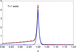
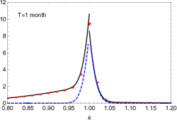
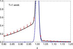
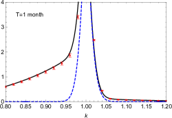
Figure 1. Asian option prices in the Merton model for maturity $T=\frac{1}{52}$ (1 week) (left) and $T=\frac{1}{12}$ (1 month) (right). The plots show the Asian put option for $k\leq 1$ and the Asian call options for $k\geq 1$ vs moneyness $k=K/S_{0}$. The solid black curve shows the analytical approximation (111), (114), and the dashed blue curve shows the diffusive component. The red dots with error bars show the results of a MC simulation described in text. The lower plots expand the lower region for added clarity.

Table 1. Numerical results for Asian call/put options with maturity $T=\frac{1}{52}$ (1 week) in the Merton jump diffusion model with parameters (120). $S_{0}=1000$.

$k=K/S_{0}$	MC price	Std Err	$a_{C,P}T$	diffusion	total
0.9	0.273	0.026	$a_{P}T=0.285$	0.0	0.285
0.95	0.378	0.032	$a_{P}T=0.388$	0.0	0.388
1.0	4.244	0.041	$a_{P}T=0.517$	4.025	4.542
1.0	4.254	0.022	$a_{C}T=0.041$	4.025	4.066
1.05	0.027	0.009	$a_{C}T=0.027$	0.0	0.027
1.1	0.018	0.008	$a_{C}T=0.018$	0.0	0.018

6.2. Double Exponential Jump model

Next we consider the pricing of Asian options under the double exponential model (82) [32]. We use similar model parameters as in [10]

(121) $$S_{0}=1000,\quad r=0.0,\quad\alpha=0.6,\quad q_{1}=1-\alpha=0.4,\quad\eta_{1}=\eta_{2}=25.$$

The intensity parameter is chosen as $\lambda=3$. We note that the parameters $\eta_{1},\eta_{2}$ satisfy the condition $\eta_{1},\eta_{2}>2$ which is required by Assumption 1.

In Figure 2 we compare the short-maturity asymptotic result of Proposition 17 against a Monte Carlo simulation of the model, in the limit $\sigma=0$ of a pure jump model. The Asian option maturity is taken as $T=1/52$ (1 week), $T=1/12$ (1 month), $T=1/2$ (6 months) and $T=1$ (1 year). The MC simulation used 100k paths. The agreement is good for $T\leq 1/12$, and the errors become larger as the maturity is increased.

In Table 2 we consider also the impact of a diffusive component with volatility $\sigma$ taking values in $0.1-0.5$ on an Asian option with maturity $T=\frac{1}{52}$. As discussed, our analytical approximation has a two-fold ambiguity at the ATM point, due to the discontinuity of the $a_{C}/a_{P}$ jump coefficients at this point. The two values are shown in Table 2 as $P/C$. For $\sigma=0$ the agreement between the theoretical approximation based on the short-maturity expansion and the MC simulation is reasonably good for strikes sufficiently far away from the ATM point. As the volatility $\sigma$ increases, the diffusive component starts to dominate the ATM Asian option price. Also the discontinuity of the analytical approximation decreases (in relative value), and the agreement with the MC simulation improves.

Table 2. Asian options pricing in the double exponential jump model with parameters (121) including also a diffusive component with volatility $\sigma$. $S_{0}=1000,T=1/52$.

$\sigma$	$k$	theory	MC price	Std Err	$\sigma$	$K$	theory	MC price	Std Err
0	0.9	0.010	0.014	0.003	0.3	0.9	0.010	0.015	0.003
0	0.95	0.061	0.064	0.006	0.3	0.95	0.194	0.217	0.008
0	1	0.444/0.721	0.698	0.014	0.3	1	10.03/10.30	9.782	0.046
0	1.05	0.128	0.124	0.009	0.3	1.05	0.326	0.370	0.013
0	1.1	0.032	0.041	0.007	0.3	1.1	0.032	0.042	0.006
0.1	0.9	0.010	0.007	0.002	0.4	0.9	0.014	0.023	0.003
0.1	0.95	0.061	0.062	0.005	0.4	0.95	0.766	0.782	0.015
0.1	1	3.64/3.91	3.591	0.020	0.4	1	13.22/13.50	13.033	0.059
0.1	1.05	0.173	0.125	0.009	0.4	1.05	1.059	1.066	0.019
0.1	1.1	0.032	0.030	0.005	0.4	1.1	0.047	0.064	0.006
0.2	0.9	0.010	0.009	0.002	0.5	0.9	0.056	0.062	0.004
0.2	0.95	0.064	0.078	0.007	0.5	0.95	1.874	1.856	0.023
0.2	1	6.83/7.11	6.721	0.032	0.5	1	16.41/16.69	16.113	0.073
0.2	1.05	0.213	0.142	0.010	0.5	1.05	2.380	2.400	0.030
0.2	1.1	0.032	0.030	0.005	0.5	1.1	0.162	0.185	0.009

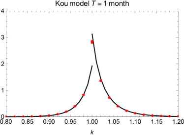
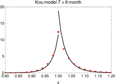
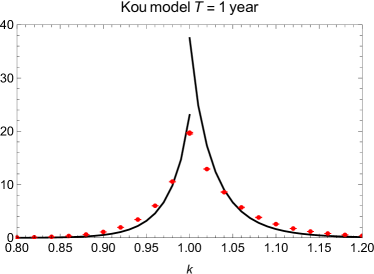
Figure 2. Asian option pricing in the double exponential model with zero diffusive volatility. The plots show $a_{P}(K)T$ (with $K/S_{0}\leq 1$) and $a_{C}(K)T$ (with $K/S_{0}\geq 1$) vs $k=K/S_{0}$ for several maturities (solid black). The red dots show the results of a MC simulation with $N_{MC}=10^{5}$ paths and $N=100$ time steps. Model parameters are as in (121).

6.3. Variance Gamma model

We present in this section test results for Asian options in the Variance Gamma model. For this test we use the model parameters

(122) $$\sigma=0.4344\,,\quad\nu=0.1083\,,\quad\theta=-0.3726\,,\quad\eta=0.0051\,,$$

and $r=q=0$. These parameters were obtained in [15] from a nonlinear square estimation from option prices on IBM stock with 1 month maturity. They calibrated to an extended version of the model of the form $S_{t}=\hat{S}_{t}e^{X_{t}^{\text{VG}}-\mu t}$ with $\hat{S}_{t}=S_{0}e^{\eta\hat{W}_{t}+(r-q-\frac{1}{2}\eta^{2})t}$ a geometric Brownian motion independent of the VG process, with volatility $\eta$. Expressed in CGMY notations using (98) these parameters read $M=12.062,G=8.113,C=9.234$. It is clear that the condition (99) is satisfied by these parameters.

Table 3 shows the short-maturity asymptotic prediction for the Asian call option in the VG model from Prop. 21, comparing with MC simulations with several option maturities. The MC simulation used 100k paths and was performed in discrete time with $N=100$ time steps. The comparison is meaningful only away from the ATM point, as the short maturity result of Prop. 21 holds only for OTM options. The agreement is good for maturities up to 1 week. A graphical representation of the results for $T=\frac{1}{52}$ and $T=\frac{1}{12}$ is shown in Figure 3, for both call and put OTM Asian options. From this plot we observe again good agreement for the shorter maturity of 1 week.

Extending the applicability of the short maturity expansion to longer maturities requires that the $O(T^{2})$ is included as well. It is possible that these corrections can be computed using an extension of the method proposed in [22] for European options in exponential Lévy models.

Table 3. Numerical results for Asian call options in the VG model with parameters (122). The second column is the short maturity asymptotic result from Prop. 21, and columns 3-5 show $1000\frac{1}{T}C_{A}(T)$ for several maturities, obtained by MC simulation as described in text.

$k=K/S_{0}$	short maturity	$T=\frac{1}{252}$	$T=\frac{1}{52}$	$T=\frac{1}{12}$
1.00	399.55	$490.9\pm 7.8$	$410.5\pm 3.5$	$286.5\pm 1.7$
1.02	166.79	$162.6\pm 6.2$	$171.5\pm 2.9$	$178.6\pm 1.5$
1.04	96.93	$94.8\pm 5.1$	$103.3\pm 2.4$	$118.9\pm 1.3$
1.06	61.53	$59.7\pm 4.3$	$67.2\pm 2.0$	$82.2\pm 1.1$
1.08	41.06	$39.9\pm 3.7$	$45.7\pm 1.7$	$58.4\pm 1.0$
1.10	28.36	$27.8\pm 3.2$	$31.9\pm 1.4$	$42.4\pm 0.8$
1.20	6.00	$6.7\pm 1.7$	$6.62\pm 0.7$	$10.3\pm 0.4$

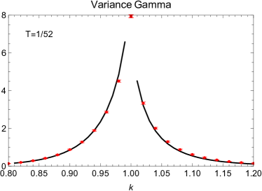
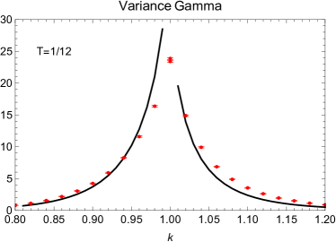
Figure 3. Asian option pricing in the Variance Gamma model. The solid black curves show the leading short-maturity asymptotic result of Proposition 21, and the red dots show the results of the MC simulation described in text. The Asian option has maturity $T=1/52$ (left) and $T=1/12$ (right). Model parameters are as in (122) and $S_{0}=1000$.

6.4. Numerical tests for floating strike Asian options

We present in this section numerical tests for the short-maturity asymptotics of floating strike Asian options. For simplicity we restrict these tests to the Merton jump-diffusion model for which the explicit result for the short-maturity asymptotics was presented in Proposition 16.

The floating strike Asian options are particular cases of the so-called “generalized Asian options” with payoff $(\kappa S_{T}-A_{T}-K)^{+}$ (call) and $(A_{T}-\kappa S_{T}-K)^{+}$ (put), corresponding to $K=0$. The analytical approximation proposed in this paper (see (111), (114)) is not appropriate for these options, as the underlying asset $B_{T}:=\kappa S_{T}-A_{T}$ is not positive definite. Thus the Black-Scholes form of the diffusive component cannot be used. A more appropriate treatment would use a Bachelier pricing formula for the diffusive component, similar to the approach proposed in Section 4.3 of [43] for the generalized Asian options in local volatility models.

We present here a direct test of the short-maturity asymptotic result for OTM floating strike Asian options. We compare in Table 4 the asymptotic result of Prop. 16 (second column) for $1000\frac{1}{T}P_{f}(T)$ against MC simulation results with several maturities from $T=\frac{1}{252}$ (one day) to $T=\frac{1}{12}$ (1 month). For the test we use the same model parameters as in (120). The parameters of the MC simulation are the same as above. The MC results are in good agreement with the OTM asymptotic prediction in the second column, for values of $\kappa$ sufficiently different from 1.

Table 4. Numerical results for floating strike Asian put options in the Merton model with parameters (120). The table shows $1000\frac{1}{T}P_{f}(\kappa,T)$ for several maturities. The second column gives the short maturity asymptotic result, and the remaining columns show MC simulation results.

$\kappa$	short maturity	$T=\frac{1}{252}$	$T=\frac{1}{52}$	$T=\frac{1}{12}$
1.0	26.904	$476.50\pm 4.86$	$223.12\pm 2.19$	$113.57\pm 1.03$
1.02	25.033	$26.19\pm 4.24$	$29.43\pm 1.93$	$43.90\pm 0.95$
1.04	23.335	$24.41\pm 4.07$	$23.34\pm 1.86$	$25.52\pm 0.90$
1.06	21.774	$22.74\pm 3.90$	$21.75\pm 1.79$	$21.88\pm 0.87$
1.08	20.332	$21.18\pm 3.74$	$20.32\pm 1.72$	$20.35\pm 0.84$
1.10	18.995	$19.75\pm 3.58$	$18.98\pm 1.66$	$19.07\pm 0.81$
1.12	17.754	$18.36\pm 3.43$	$17.74\pm 1.60$	$17.87\pm 0.78$
1.14	16.598	$17.05\pm 3.29$	$16.58\pm 1.54$	$16.76\pm 0.75$
1.16	15.523	$15.90\pm 3.16$	$15.49\pm 1.49$	$15.73\pm 0.72$
1.18	14.520	$14.83\pm 3.02$	$14.50\pm 1.43$	$14.76\pm 0.70$
1.20	13.584	$13.77\pm 2.90$	$13.60\pm 1.38$	$13.87\pm 0.67$

References

• [1] Alòs, E., Léon, J. and J. Vives. (2007). On the short-time behavior of the implied volatility for jump-diffusion models with stochastic volatility. Finance and Stochastics. 11, 571-589.
• [2] Alòs, E., Nualart, E. and M. Pravosud (2022). On the implied volatility of Asian options under stochastic volatility. arXiv: 2208.01353[q-fin]
• [3] Alziary, B., Decamps, J. P. and P. F. Koehl. (1997). A PDE approach to Asian options: Analytical and Numerical evidence. Journal of Banking and Finance. 21, 613-640.
• [4] Andersen, L. and J. Andreasen. (2000). Jump diffusion process: Volatility smile fitting and numerical methods for option pricing. Review of Derivatives Research. 4, 231-262.
• [5] Arguin, L.P., N.-L. Lin and T.-H. Wang (2018). Most-likely path in Asian option pricing under local volatility models. International Journal of Theoretical and Applied Finance, 21(5), 1850029.
• [6] Bayraktar, E. and H. Xing. (2011). Pricing Asian options for jump diffusion. Mathematical Finance. 21, 117-143.
• [7] Benhamou, E., Gobet, E. and M. Miri. (2009). Smart expansion and fast calibration for jump diffusions. Finance and Stochastics. 13, 563-589.
• [8] Benhamou, E. (2002). Fast Fourier Transform for Discrete Asian Options. Journal of Computational Finance. 6, 49-61.
• [9] Boyarchenko, S.I. and S. Levendorskii. (2002). Non-Gaussian Merton-Black-Scholes Theory. Advanced Series on Statistical Science and Applied Probability. Vol.9, World Scientific Publishing Co., River Edge NJ, 2002.
• [10] Cai, N. and S. G. Kou. (2012). Pricing Asian options under a hyper-exponential jump diffusion model. Operations Research. 60(1), 64-77.
• [11] Cai, N. and C. Li and C. Shi. (2014). Closed-form expansions of discretely-monitored Asian options in diffusion models. Mathematics of Operations Research. 39(3), 789-822.
• [12] Cai, N., Y. Song and S. G. Kou. (2015). A general framework for pricing Asian options under Markov processes. Operations Research. 63(3), 540-554.
• [13] Cui, Z., Lee, C. and Y. Liu. (2018). Single-transform formulas for pricing Asian options in a general approximation framework under Markov processes, European Journal of Operational Research. 266(3), 1134-1139.
• [14] Carverhill, P. and M. Clewlow. (1990). Flexible convolution. Risk. 3(4), 25-29.
• [15] Carr, P., Geman, H., Madan, D. and M. Yor. (2002). The fine structure of asset returns: An empirical investigation. Journal of Business. 75, 303-325.
• [16] Carr, P. and M. Schröder. (2003). Bessel processes, the integral of geometric Brownian motion, and Asian options. Theory of Probability and its Applications. 48, 400-425.
• [17] Carr, P. and L. Wu. (2003). What type of process underlies options? A simple robust test. The Journal of Finance 58(6), 2581-2610.
• [18] Chow, C. S. and H. J. Lin. (2006). Asian options with jumps. Statistics and Probability Letters. 76, 1983-1993.
• [19] Dembo, A. and O. Zeitouni. Large Deviations Techniques and Applications. 2nd Edition, Springer, New York, 1998.
• [20] Dufresne, D. (2005). Bessel processes and a functional of Brownian motion, in M. Michele and H. Ben-Ameur (Ed.), Numerical Methods in Finance, 35-57, Springer, 2005.
• [21] Figueroa-López, J. E. (2008). Small-time moment asymptotics for Lévy models. Statistics and Probability Letters. 78, 3355-3365.
• [22] Figueroa-López, J. E. and M. Forde. (2012). The small-maturity smile for exponential Lévy models. SIAM Journal on Financial Mathematics. 3, 33-65.
• [23] Figueroa-López, J. E. and S. Ólaffson. (2015). Short-time asymptotics for the implied volatility in a stochastic volatility model with Lévy jumps. arxiv:1502.02595[q-fin.MF]
• [24] Foschi, P., Pagliarani, S. and A. Pascucci (2013). Approximations for Asian options in local volatility models. Journal of Computational and Applied Mathematics. 237, 442-459.
• [25] Fu, F., Madan, D. and T. Wang. (1998). Pricing continuous time Asian options: a comparison of Monte Carlo and Laplace transform inversion methods. Journal of Computational Finance. 2, 49-74.
• [26] Fusai, G. (2004). Pricing Asian options via Fourier and Laplace transforms. Journal of Computational Finance. 7(3), 87-106.
• [27] Fusai, G. and A. Meucci. (2008). Pricing discretely monitored Asian options under Lévy processes, Journal of Banking and Finance. 32(10):2076-2088.
• [28] Geman, H. and M. Yor. (1993). Bessel processes, Asian options and perpetuities. Mathematical Finance. 3, 349-375.
• [29] Gobet, E. and M. Miri. (2014). Weak approximation of averaged diffusion processes. Stochastic Processes and their Applications. 124, 475-504.
• [30] Hackmann, D. and A. Kuznetsov. (2014). Asian options and meromorphic Lévy processes. Finance and Stochastics. 18, 825-844.
• [31] Henderson, V. and R. Wojakowski. (2002). On the equivalence of floating and fixed-strike Asian options, Journal of Applied Probability. 39, 391-394.
• [32] Kou, S.G. (2002). A jump diffusion model for option pricing. Management Science. 48, 1086-1101.
• [33] Kou, S. G. and H. Wang. (2004). Option pricing under a double exponential jump diffusion model. Management Science. 50, 1178-1192.
• [34] Kyriakou, I., P.K. Pouliasis and N.C. Papapostolou. (2016). Jumps and stochastic volatility in crude oil prices and advances in average options pricing. Quantitative Finance. 16, 1859-1873.
• [35] Madan, D.P. and E. Seneta. (1990). The VG for share market returns. Journal of Business. 63, 511-524.
• [36] Madan, D.P., Carr, P. and E. Chang. (1998). The variance gamma process and option pricing. European Finance Review. 2, 79-105.
• [37] Merton, R.C. (1976). Option pricing when the underlying stock returns are discontinuous. Journal of Financial Economics. 3, 125-144.
• [38] Muhle-Karbe, J. and M. Nutz. (2011). Small-time asymptotics of option prices and first absolute moments. Journal of Applied Probability. 48, 1003-1020.
• [39] Pagliarani, S. and A. Pascucci. (2013). Local stochastic volatility with jumps: analytical approximations. International Journal of Theoretical and Applied Finance. 16(8), 1350050.
• [40] Pirjol, D. and L. Zhu (2016). Short maturity Asian options in local volatility models. SIAM Journal on Financial Mathematics. 7(1), 947-992.
• [41] Pirjol, D. and L. Zhu. (2016). Discrete sums of geometric Brownian motions, annuities and Asian options. Insurance: Mathematics and Economics. 70, 17-36.
• [42] Pirjol, D. and L. Zhu. (2019). Short maturity Asian options for the CEV model. Probability in the Engineering and Informational Sciences. 33, 258-290.
• [43] Pirjol, D., J. Wang and L. Zhu. (2019). Short maturity forward start Asian options in local volatility models. Applied Mathematical Finance. 26(3), 187-221.
• [44] Rogers, L. and Z. Shi. (1995). The value of an Asian option. Journal of Applied Probability. 32, 1077-1088.
• [45] Varadhan, S. R. S. (1967). Diffusion processes in a small time interval. Communications on Pure and Applied Mathematics. 20, 659-685.
• [46] Varadhan, S. R. S. Large Deviations and Applications, SIAM, Philadelphia, 1984.
• [47] Vecer, J. (2001). A new PDE approach for pricing arithmetic average Asian options. Journal of Computational Finance. 4, 105-113.
• [48] Vecer, J. and M. Xu. (2002). Unified Asian pricing. Risk. 15, 113-116.