Supplementary material of DebSDF: Delving into the Details and Bias of Neural Indoor Scene Reconstruction

1 Large Curvature Radius Situation

The SDF mapping function $y(t)$ can be simplified to $y(t)=s(t)/|\cos\theta(t)|$ when the absolute value of the curvature radius is a very large number. This corresponds to the situation that the ray intersects with the planar surface. This approximation comes from the fact that the limit of $y(t)$ is $s(t)/|\cos\theta(t)|$ as the radius of curvature $R(\textbf{r}(t),\textbf{v})\to\infty$. We take this approximation when the absolute value of the curvature radius is large due to limitations in numerical precision.

Proof.

Since $a(t)+s(t)=R(\textbf{r}(t),\textbf{v})>0$,

$$\begin{split}\begin{aligned} \lim_{R\to\infty}y&=\lim_{R\to\infty}\left[(a+s)|\cos\theta|-\sqrt{a^{2}-(a+s)^{2}\sin^{2}\theta}\right]\\ &=\lim_{R\to\infty}\left[R|\cos\theta|-\sqrt{a^{2}-R^{2}\sin^{2}\theta}\right]\\ &=\lim_{R\to\infty}\left[\sqrt{R^{2}\cos^{2}\theta}\ -\sqrt{a^{2}-R^{2}(1-\cos^{2}\theta)}\right]\\ &=\lim_{R\to\infty}\left[\sqrt{R^{2}\cos^{2}\theta}\ -\sqrt{R^{2}\cos^{2}\theta-R^{2}+a^{2}}\right]\end{aligned}\end{split}$$

Let $f(x)=\sqrt{x}$,

$$\begin{split}\begin{aligned} \lim_{R\to\infty}y=\lim_{R\to\infty}\left[\sqrt{R^{2}\cos^{2}\theta}\ -\sqrt{R^{2}\cos^{2}\theta-R^{2}+a^{2}}\right]\\ =\lim_{R\to\infty}\left[f(R^{2}\cos^{2}\theta)\ -f(R^{2}\cos^{2}\theta-R^{2}+(R-s)^{2})\right]\\ \end{aligned}\end{split}$$

Without loss of generality, assuming that $s>0$, we know $(R-s)^{2}<R^{2}$. Then we get,

$$R^{2}\cos^{2}\theta>R^{2}\cos^{2}\theta-R^{2}+(R-s)^{2}.$$

Assuming that there is a $\xi$ suffice the inequality that

$$R^{2}\cos^{2}\theta-R^{2}+(R-s)^{2}<\xi<R^{2}\cos^{2}\theta$$

According to Lagrange’s mean value theorem, we get

$$\begin{split}\begin{aligned} &f(R^{2}\cos^{2}\theta)-f(R^{2}\cos^{2}\theta-R^{2}+(R-s)^{2})\\ &=f^{\prime}(\xi)(R^{2}-(R-s)^{2})\\ &=f^{\prime}(\xi)(2Rs-s^{2})\end{aligned}\end{split}$$

Therefore we know that,

$$\begin{split}\begin{aligned} &\lim_{R\to\infty}\left[f(R^{2}\cos^{2}\theta)\ -f(R^{2}\cos^{2}\theta-R^{2}+(R-s)^{2})\right]\\ &=\lim_{R\to\infty}f^{\prime}(\xi)(2Rs-s^{2})=\cfrac{2Rs-s^{2}}{2\sqrt{\xi}}\\ \end{aligned}\end{split}$$

Since we know that

$$\begin{split}\begin{aligned} &R^{2}\cos^{2}\theta-R^{2}+(R-s)^{2}\\ &=R^{2}\cos^{2}\theta-2Rs+s^{2}<\xi<R^{2}\cos^{2}\theta\end{aligned}\end{split}$$

Then $\xi$ can be denoted as $R^{2}cos^{2}\theta+o(R^{2})$. Here $o(R^{2})$ is the lower order infinity of $R^{2}$.

Finally, we prove the limit of $y$ approaches $s/|cos\theta|$, which is the same as TUVR [zhang2023towards].

$$\begin{split}\begin{aligned} \lim_{R\to\infty}y&=\lim_{R\to\infty}\cfrac{2Rs-s^{2}}{2\sqrt{R^{2}\cos^{2}\theta+o(R^{2})}}\\ &=\lim_{R\to\infty}\cfrac{Rs}{\sqrt{R^{2}\cos^{2}\theta+o(R^{2})}}\\ &=\cfrac{s}{\sqrt{\cos^{2}\theta+\cfrac{o(R^{2})}{R^{2}}}}=\cfrac{s}{|\cos\theta|}\end{aligned}\end{split}$$

The proof process is very similar when $s<0$ and $y$ also converge to $s/|\cos\theta|$ in this situation. ∎

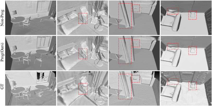
Figure 1: The qualitative experiments to evaluate the efficiency of the progressive manner in our bias-aware SDF to density transformation (Sec. 3.5). The ”Non-Prog” indicates applying the bias-aware SDF to density transformation without progressive growing. The progressive manner can make the optimization of thin and detailed structures more stable.

2 Progressively Warm-up of Bias-aware SDF to Density Transformation

As aforementioned before, we design the bias-aware SDF to density transformation in a progressive manner to ensure the stabilization of training. In this subsection, we conduct quantitative and qualitative experiments to validate the efficiency of this design. As shown in Table. I, the ”Non-Prog” indicates applying the bias-aware SDF to density transformation without progressive warm-up. It can be observed that this progressive manner achieves significant improvement by 5.35 F-score.

The qualitative results are shown in Fig. 1. Though applying the bias-aware SDF to density transformation without the progressive manner can still reconstruct the texture-less region well, the reconstruction of detailed and small structures seriously degraded, such as the tables, chairs, and the curtain. These experimental results prove that the designed progressive manner can make the training robust.

TABLE I: The quantitative results on the ScaNet dataset. The ”Non-Prog” indicates applying the bias-aware SDF to density transformation without progressive warm-up, and the ”Prog” indicates our proposed model.

	Chamfer	F-score	Normal C
Non-Prog	0.042	73.19	89.85
Prog	0.038	78.54	90.21

3 Time Consumption

The time consumed in the training phase of each method is shown in the Table. II. Though the implementation of MonoSDF [yu2022monosdf] and our method are both based on the VolSDF [yariv2021volume], our method consumes more time for training. The reason is that our model needs to compute the SDF gradient and uncertainty score of each point at the point sampling for the opacity estimation. Apply other point sampling algorithms, such as the sampling based on proposal MLP [barron2022mip], may eliminate this negative impact.

TABLE II: The time-consuming of different methods. All methods are implemented on NVIDIA Geforce RTX 2080ti. The * indicates applying the hash encoding feature grids.

Methods	NeuRIS	MonoSDF	Ours	MonoSDF*	Ours*
Times (h)	11	26	31	17	21