Exact mobility edges in finite-height Wannier-Stark ladders

Abstract

We investigate the single-particle localization transition in one-dimensional Wannier-Stark ladders with either a linear potential or a mosaic potential with spacing $\kappa=2$. In both cases, we exactly determine the mobility edges separating the Wannier-Stark localized states from extended states for a finite potential height. Especially in the latter case, we obtain mobility edges through a revised Lyapunov exponent, and demonstrate a rich phase diagram with extended states, weakly Wannier-Stark localized states, and strongly Wannier-Stark localized states. Our results also exhibit that mobility edges are highly dependent on the height of the ladder and extended states only survive at $E\approx 0$ for the high ladder. Finally, we perform the simulation of the dynamical evolution for possible experimental observations. These interesting features will shed light on the study of localization phenomena in disorder-free systems.

I Introduction

Anderson localization Anderson (1958) is well-known as the phenomenon that the diffusion of the wave decays exponentially in disordered systems. It provides a foundational understanding of the insulating property of materials containing impurities. The scaling theory shows that Anderson localization is dimension-dependent Abrahams et al. (1979); Thouless (1974); Evers and Mirlin (2008); Mott (1987). In one- and two-dimensional systems without any symmetry, all states are Anderson localized states in the presence of arbitrarily weak random disorder Abrahams et al. (1979); Thouless (1974). While in three dimensions, there is a localization transition from extended states to Anderson localized states as the disorder strength increases. In the transition region, Anderson localized states and extended states coexist, and they are divided by critical energies, dubbed as mobility edges Evers and Mirlin (2008). Since then, various randomly disordered systems and quasi-periodic (quasi-randomness) systems have been discovered to display the existence of mobility edges Aubry and André (1980); Harper (1955); Das Sarma et al. (1988); Wang et al. (2020); Liu et al. (2020); Liu and Guo (2018); Li et al. (2017); Xia et al. (2022); Wei et al. (2019); Ganeshan et al. (2015); Goncalves et al. (2023); Lin et al. (2023); Liu et al. (2022); Deng et al. (2019); Biddle and Das Sarma (2010); Zeng et al. (2023), and part of them have been observed in the experiments Semeghini et al. (2015); Pasek et al. (2017); Lüschen et al. (2018); Lin et al. (2022).

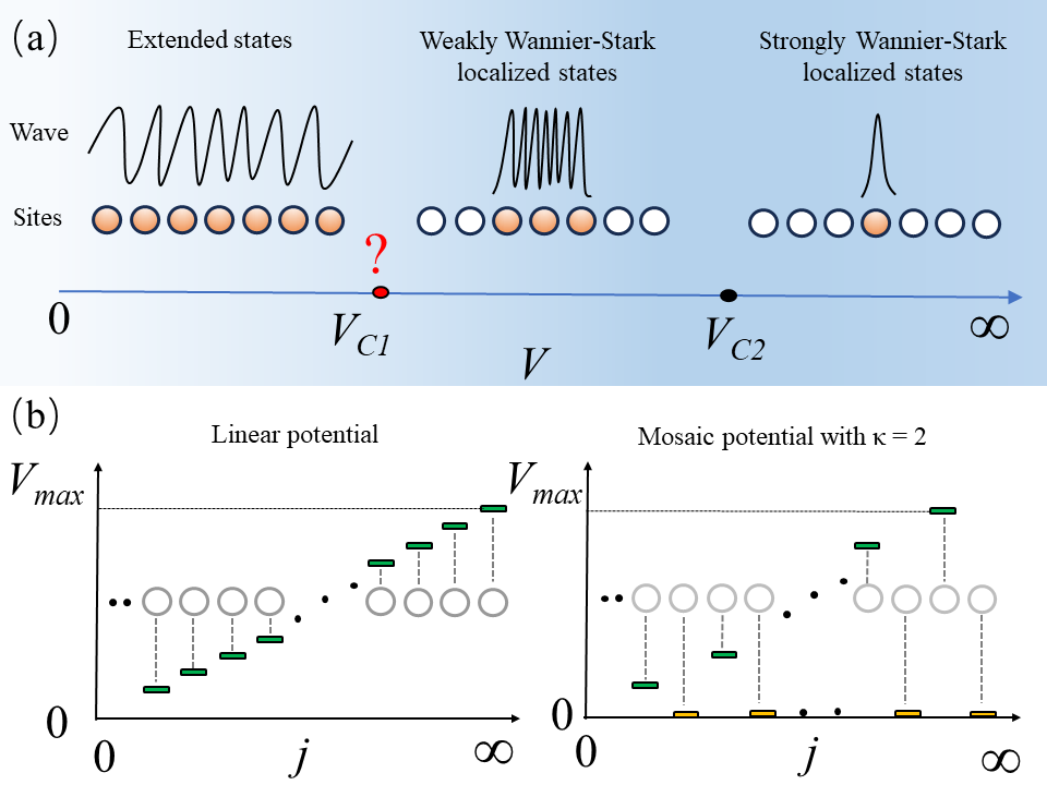
Figure 1: The schematic plot of wave functions and potentials. (a) Typical wave functions for extended states, weakly Wannier-Stark localized states, and strongly Wannier-Stark localized states. (b) The linear potential and the mosaic potential with spacing $\kappa=2$. In (a), circles represent lattice sites and orange filled ones represent occupied sites by the wave function. $V_{1}$ and $V_{2}$ indicate the transition points from extended states to weakly Wannier-Stark localized states and from weakly to strongly Wannier-Stark localized states, respectively. In (b), $j$ is the site index and $V_{max}$ represents the maximum value of the potential. The green and yellow lines indicate that the potential energy is non-zero and zero, respectively.

Recently, it has been shown that mobility edges also exist in disorder-free systems with mosaic modulations Dwiputra and Zen (2022); Qi et al. (2023); Liu (2022); Gao et al. (2023). By utilizing the Avila’s theory Avila (2015), Ref. Dwiputra and Zen (2022) calculates the Lyapunov exponent to acquire the localization transition point $V/t=2$ for the system with a linear potential, where $t$ and $V$ are the hopping energy and the strength of the linear potential, respectively. However, this result seems to violate the fact that all states are Wannier-Stark localized states for arbitrarily finite $V$ in the thermodynamic limit Hartmann et al. (2004); Glück et al. (2002); van Nieuwenburg et al. (2019); Wei et al. (2022). To clarify this misleading, we should refer to the definition of Wannier-Stark localization. For the model in the presence of a linear potential, the eigenstates are the well-known Wannier-Stark states $|\Psi_{m}\rangle=\sum_{j}\mathcal{J}_{j-m}(2t/V)|j\rangle$  Fukuyama et al. (1973a), where $\mathcal{J}_{j-m}$ are the Bessel functions of the first kind, $j$ and $m$ represent the site index and energy level index, respectively. The properties of the Bessel functions show that $\mathcal{J}_{j-m}$ are mainly localized in the interval $|m-j|<2t/V$ and decay as $\mathcal{J}_{j}(2t/V)\sim(2t/V)^{j}$ outside this interval van Nieuwenburg et al. (2019). In the thermodynamic limit with the system size $L\rightarrow\infty$, $|m-j|<2t/V\ll L$ for arbitrarily finite $V$, thus all states are Wannier-Stark localized states. Here we explicitly define that the strongly Wannier-Stark localized state corresponds to the wave function localizing in about a single site Qi et al. (2023); Liu (2022), whereas the weakly Wannier-Stark localized state corresponds to the wave function localizing within an interval much larger than one site Hartmann et al. (2004); Glück et al. (2002); van Nieuwenburg et al. (2019); Wei et al. (2022); Longhi (2023), as shown in Fig. 1 (a). Hence, the localization transition derived from $V/t=2$ in Ref. Dwiputra and Zen (2022) actually refers to strong Wannier-Stark localization, and the “mobility edge” provided in it separates strongly Wannier-Stark localized states from other states, rather than Wannier-Stark localized states from extended states. In this work, we mainly focus on identifying exact mobility edges separating Wannier-Stark localized states from extended states in finite-height Wannier-Stark ladders.

II Model

We investigate the diffusion behavior of a quantum particle in a disorder-free chain with open boundary conditions, which is described by the following Schrödinger equation Berezin and Shubin (2012)

$$t\left(\psi_{j+1}+\psi_{j-1}\right)+V_{j}\psi_{j}=E\psi_{j},$$ (1)

where $\psi_{j}$ is the amplitude of the wavefunction at the site $j$. $E$ is the eigenvalue. We set the nearest-neighbor hopping strength $t\equiv 1$ as the energy unit and $V_{j}$ is the site-dependent potential, which reads

$$V_{j}=\begin{cases}Vj,&j=\kappa i\\ 0,&\text{ otherwise }\end{cases},$$ (2)

where $V$ is the strength of the linear potential. $\kappa$ adjusts the spacing of sites with the non-zero potential. Typically, we choose $\kappa=1$ and $\kappa=2$ in this work, corresponding to the linear potential and the mosaic potential Wang et al. (2020); Dwiputra and Zen (2022), respectively. The schematic plots of potentials are shown in Fig. 1 (b). $i=0,1,2,\ldots,(N-1)$ represents the location of the supercell. Each supercell includes $\kappa$ sites, thus the chain length is expressed as $L=\kappa N$. The maximum value of the potential in the supercell is defined as $V_{max}=\kappa V(N-1)$.

For $\kappa=1$, Eq. (1) is reduced to the Wannier-Stark model Wannier (1962); Fukuyama et al. (1973b), whose eigenstates are all Wannier-Stark localized states for arbitrarily finite $V$ Hartmann et al. (2004); Glück et al. (2002); van Nieuwenburg et al. (2019); Wei et al. (2022). For $\kappa=2$, disorder-free mobility edges are reported recently Dwiputra and Zen (2022). Remarkably, these two models have already been realized in experiments in the superconducting qubit and nanophotonic device systems Guo et al. (2021); Gao et al. (2023).

III Lyapunov exponent and mobility edges

We start from Eq. (1) and transform it into the transfer matrix form as

$$\left[\begin{array}[]{c}\psi_{j+1}\\ \psi_{j}\end{array}\right]=T_{j}\left[\begin{array}[]{c}\psi_{j}\\ \psi_{j-1}\end{array}\right],$$ (3)

where $T_{j}$ is given by

$$T_{j} =\left(\begin{array}[]{cc}E-V_{j}&-1\\ 1&0\end{array}\right).$$ (4)

For convenience, we abbreviate Eq. (3) as $\Psi_{j}=T_{j}\Psi_{j-1}$. The transfer matrix of the supercell $\tilde{T}_{i}$ is composed of $\kappa$ small transfer matrices ${T}_{j}$, thus it can be written as

$$\tilde{T}_{i} =\prod_{j=\kappa i}^{\kappa i+\kappa-1}\left(\begin{array}[]{cc}E-V_{j}&-1\\ 1&0\end{array}\right)$$ (5)

$$=\left(\begin{array}[]{cc}E-V\kappa i&-1\\ 1&0\end{array}\right)\left(\begin{array}[]{cc}E&-1\\ 1&0\end{array}\right)^{\kappa-1}.$$

The Lyapunov exponent indicates the exponential rate of growth of the transfer matrix product, which is defined as

$$\gamma(E) =\lim_{L\rightarrow\infty}\frac{1}{L}\ln(||\prod_{j=0}^{L-1}T_{j}||)$$ (6)

$$=\lim_{L\rightarrow\infty}\frac{1}{L}\ln(||\prod_{i=0}^{N-1}\tilde{T}_{i}||),$$

where $||$ $\cdot$ $||$ is the norm of the matrix, determined by the maximum of the absolute value of eigenvalues. For localized states, $\gamma(E)>0$, whereas for non-localized states $\gamma(E)=0$ Li et al. (2017); Zhang and Zhang (2022). The Lyapunov exponent is widely used in the studies of Anderson localization and mobility edges Li et al. (2017); Zhang and Zhang (2022); Wang et al. (2021); Cai and Yu (2022); Jiang et al. (2023); Liu et al. (2021a, b). In the present work, we show that the Lyapunov exponent is also a good indicator of the Wannier-Stark localization transition. The first approximation we make is that when the height of the Wannier-Stark ladder is finite, $\tilde{T}_{i}\approx\tilde{T}_{i+1}$ for $L\rightarrow\infty$ according to Eq. (5), hence the transfer matrix product can be converted to $||\prod_{i=0}^{N-1}\tilde{T}_{i}||=||\phi_{N-1}\Lambda_{N-1}\phi_{N-1}^{\dagger}\phi_{N-2}\Lambda_{N-2}\phi_{N-2}^{\dagger}\ldots\phi_{0}\Lambda_{0}\phi_{0}^{\dagger}||\approx||\phi_{N-1}\prod_{i=0}^{N-1}\Lambda_{i}\phi_{0}^{\dagger}||\approx||\prod_{i=0}^{N-1}\Lambda_{i}||=\prod_{i=0}^{N-1}||\tilde{T}_{i}||$, where $\phi$ and $\Lambda$ are matrices composed of the eigenstates and eigenvalues of the transfer matrix $\tilde{T}$, respectively. Thus we obtain that the Lyapunov exponent is approximated as

$$\gamma(E)\approx\lim_{L\rightarrow\infty}\frac{1}{L}\ln(\prod_{i=0}^{N-1}||\tilde{T}_{i}||).$$ (7)

By a direct computation, $\gamma(E)$ for $\kappa=1$ and $\kappa=2$ can be obtained as

$$\gamma(E) \approx\lim_{L\rightarrow\infty}\frac{1}{L}\sum_{i=0}^{N-1}\ln(\text{max}\{|\varepsilon_{1}|,|\varepsilon_{2}|\})$$ (8)

$$=\lim_{L\rightarrow\infty}\frac{1}{L}\sum_{i=0}^{N-1}\Bigg{|}\ln(|\frac{-\mu+\sqrt{\mu^{2}-4}}{2}|)\Bigg{|},$$

where $\varepsilon_{1}$ and $\varepsilon_{2}$ are eigenvalues of $\tilde{T}_{i}$, $\varepsilon_{1}=1/\varepsilon_{2}$ due to the determinant $|\tilde{T}_{i}|=1$. $\mu=E-Vi$ for $\kappa=1$ and $\mu=E^{2}-2EVi-2$ for $\kappa=2$. Evidently, $\gamma(E)=0$, the condition gives $|\frac{-\mu\pm\sqrt{\mu^{2}-4}}{2}|=1$ for any $i$, which can be satisfied if $|\mu|\leq 2$ for any $i$. Since the non-zero potential is linear, $|\mu|\leq 2$ for any $i$ can be guaranteed as long as both the head ($i=0$) and end ($i=N-1$) of the ladder satisfy $|\mu|\leq 2$. Thus, according to $|\mu(0)|=|\mu(N-1)|=2$, we can obtain that mobility edges for $\kappa=1$ are at

$$E=\left\{\begin{aligned} &2,\\ &-2+V_{max},\\ \end{aligned}\right.$$ (9)

and those for $\kappa=2$ are at

$$E=\left\{\begin{aligned} &0,\\ &2,\\ &\frac{V_{max}-\sqrt{(V_{max})^{2}+16}}{2},\\ &V_{max},\\ \end{aligned}\right.$$ (10)

It needs to be emphasized that the above derivation is based on $\tilde{T}_{i}\approx\tilde{T}_{i+1}$, which requires the height of the Wannier-Stark ladder to be finite.

To verify the predictions of Eq. (9) and Eq. (10), we numerically calculate the Lyapunov exponent by the following method from the original definition Zhang and Zhang (2022)

$$\gamma(E) =\lim_{L\rightarrow\infty}\frac{1}{L}\ln(|\Psi_{L-1}|/|\Psi_{0}|)$$ (11)

$$=\lim_{L\rightarrow\infty}\frac{1}{L}\ln(\frac{|\Psi_{L-1}|}{|\Psi_{L-2}|}\frac{|\Psi_{L-2}|}{|\Psi_{L-3}|}\ldots\frac{|\Psi_{1}|}{|\Psi_{0}|})$$

$$=\lim_{L\rightarrow\infty}\frac{1}{L}\sum_{j=0}^{L-2}\ln(\frac{|\Psi_{j+1}|}{|\Psi_{j}|}),$$

where $|\Psi_{j}|=\sqrt{|\psi_{j+1}|^{2}+|\psi_{j}|^{2}}$ is the norm of the vector. In detail, we first choose a normalized vector

$$\Psi_{0}=\left(\begin{array}[]{c}\sqrt{2}/2\\ \sqrt{2}/2\end{array}\right),$$ (12)

as the initial vector and set the initial Lyapunov exponent to $\gamma(E)=0$. Then, we iterate $j$ from zero to $L-2$ to calculate the Lyapunov exponent according to Eq. (11) by the following steps:

• normalize the vector $\Psi_{j}=\Psi_{j}/|\Psi_{j}|$ at the site $j$;

• calculate the next vector $\Psi_{j+1}=T_{j+1}\Psi_{j}$ by Eq. (3);

• calculate the Lyapunov exponent $\gamma(E)=\gamma(E)+\frac{1}{L}\ln(|\Psi_{j+1}|/|\Psi_{j}|)=\gamma(E)+\frac{1}{L}\ln|\Psi_{j+1}|$, since $\Psi_{j}$ has been normalized in the first step.

IV results

Figure 2: Spectra and mobility edges as a function of $V_{max}$. Color represents the value of $\ln|\gamma(E)|$. The dark (light) color region corresponds to the extended (weakly Wannier-Stark localized) region. The value of $V_{max}$ here is far from meeting the requirements for achieving strong Wannier-Stark localization. The solid and dashed lines in red and black mark the mobility edges separating extended states from weakly Wannier-Stark localized states. (a) $\kappa=1$ and (b) $\kappa=2$. $L=500$.

The main results are shown in Fig. 2, in which we use the original Lyapunov exponent defined by Eq. (11) to characterize mobility edges. In Fig. 2 (a), we consider the linear potential for $\kappa=1$. Two mobility edges are at $E=2$ and $E=-2+V_{max}$ for $V_{max}<4$, which agrees with Eq. (9). As $V_{max}$ increases, the region of extended states is compressed gradually. For $V_{max}>4$, extended states disappear and all states in the spectrum are weakly Wannier-Stark localized states in Fig. 2 (a). Further enhancing the strength of the potential, the system enters the strong Wannier-Stark localization region, where the particle localizes in about a single lattice Dwiputra and Zen (2022); Qi et al. (2023); Liu (2022). In the thermodynamic limit, $V_{max}\rightarrow\infty$ for arbitrarily finite $V$, thus it can be concluded that arbitrarily finite $V$ can induce the system to enter the Wannier-Stark localization, which is consistent with Ref. Hartmann et al. (2004); Glück et al. (2002); van Nieuwenburg et al. (2019); Wei et al. (2022). It is worth mentioning that from the perspective of energy conservation, extended states and weakly Wannier-Stark states can also be understood as scattered states and bound states Phillips (2013), thus mobility edges can also be obtained by analyzing eigenvalues Wei et al. (2022). In Fig. 2 (b), we consider the mosaic potential for $\kappa=2$. There are four mobility edges for $V_{max}<2$, and two of them disappear for $V_{max}>2$, only $E=0$ and $E=(V_{max}-\sqrt{(V_{max})^{2}+16})/2$ survive. These two mobility edges approach each other as $V_{max}$ increases. Thus for a large $V_{max}$, extended states only exist at $E\approx 0$ and the rest of the states are all Wannier-Stark localized states.

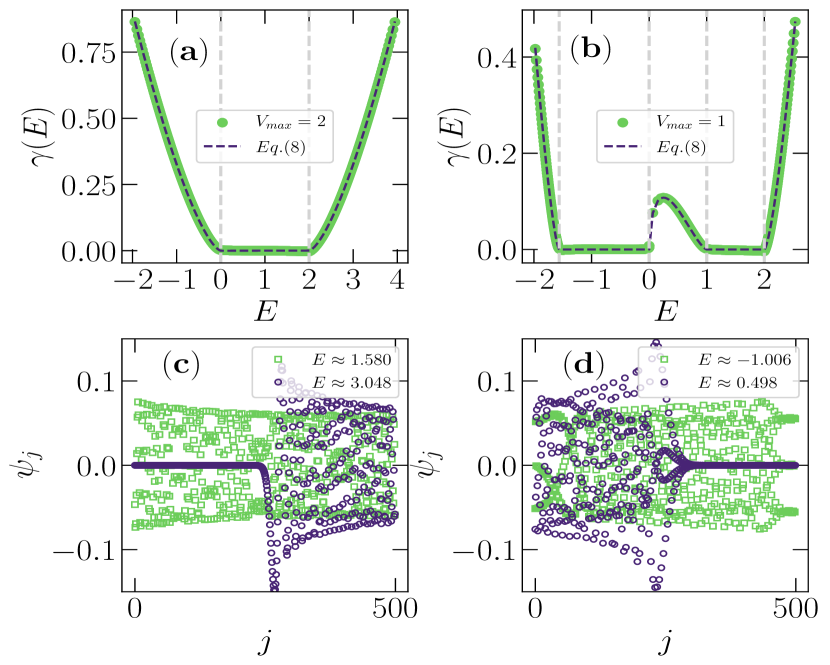
Figure 3: Lyapunov exponents $\gamma(E)$ and wave functions $\psi_{j}$ for $\kappa=1$ (left panels) and $\kappa=2$ (right panels). The grey dotted lines mark mobility edges at $E=0$ and $E=2.0$ in (a), whereas those in (b) mark mobility edges at $E=\frac{1-\sqrt{17}}{2}$, $E=0$, $E=1$ and $E=2.0$. $L=500$. $V_{max}=2.0$ in the left panels and $V_{max}=1.0$ in the right panels.

In Fig. 3, we show typical Lyapunov exponents and wave functions for $\kappa=1$ (left panels) and $\kappa=2$ (left panels). In both cases, the Lyapunov exponent $\gamma(E)=0$ for extended states, whereas $\gamma(E)>0$ for weakly Wannier-Stark localized states in Fig. 3 (a) and (b), which is consistent with its characteristics in disordered systems Li et al. (2017); Zhang and Zhang (2022). The numerical solution of the Lyapunov exponent coincides well with Eq. (8), indicating that the approximation $\tilde{T}_{i}\approx\tilde{T}_{i+1}$ is reasonable. Fig. 3 (c) and (d) exhibit that, wave functions diffuse throughout the whole chain for extended states, whereas wave functions are trapped in an interval smaller than $L$ for weakly Wannier-Stark localized states. Note that, wave functions of weakly Wannier-Stark localized states are at the opposite partitions in Fig. 3 (c) and (d), this is because the distribution of Wannier-Stark states is energy-dependent. Although wave functions of weakly Wannier-Stark localized states do not decay exponentially, the Lyapunov exponent can still indicate mobility edges well. This is due to the fact that, on the one hand, the Lyapunov exponent of extended states affected by the linear and mosaic potentials remains zero, on the other hand, the weakly Wannier-Stark localized states decay approximately exponentially at the tail van Nieuwenburg et al. (2019), providing a non-zero Lyapunov exponent.

Figure 4: Fractal dimension $D$ and its scaling analysis for $\kappa=1$ (left panels) and $\kappa=2$ (right panels). The grey dotted lines in (a) and (b) mark the same mobility edges as those in Fig. 3 (a) and (b), respectively. The legends in (c) and (d) indicate the target eigenvalue $E$ and the fractal dimension $D$ obtained by the linear fitting. The largest size in (c) and (d) is $L=25600$. $V_{max}=2.0$ in the left panels and $V_{max}=1.0$ in the right panels.

In order to more accurately describe the properties of eigenstates, we further investigate the fractal dimension of the wave function, which is associated with the inverse participation ratio (IPR), $\sum_{j}|\psi_{j}|^{4}$, and defined as

$$D=\frac{-\ln\text{(IPR)}}{\ln L},$$ (13)

In the thermodynamic limit, $D=1$ for extended states, $D=0$ for localized states, and $0<D<1$ for fractal states Aoki (1986); Huckestein (1995, 1995); De Luca et al. (2014), i.e., critical states in other works Zhou et al. (2023); Mirlin et al. (2006); Janssen (1998); Dubertrand et al. (2014). Evidently, the regions with larger fractal dimensions in Fig. 4 (a) and (b) are consistent with the regions where $\gamma(E)=0$ in Fig. 3 (a) and (b). And the discontinuous variations in the derivative of $D$ exactly correspond to the mobility edges marked by grey dotted lines. Additionally, the size-effect analyses in Fig. 4 (c) and (d) show that $D\approx 1.0$ for extended states, whereas $0<D<1$ for weakly Wannier-Stark localized states. By the linear fitting, we find that Eq. (13) for the finite size needs to be modified as $D=(-\ln(\text{IPR})+\delta)/\ln L$, where $\delta$ is a correction value. For $L\rightarrow\infty$, $\delta/\ln L\rightarrow 0$, thus the revised equation reduces to Eq. (13) in the thermodynamic limit. The fractal dimension for weakly Wannier-Stark localized states can be approximately written as $D=\ln\Delta/\ln L$, where $\Delta$ is the width of the local interval. According to the definition of weakly Wannier-Stark localized states, $1<\Delta<L$, thus $0<D<1$ for weakly Wannier-Stark localized states. In Fig. 4 (c) and (d), the IPRs of weakly Wannier-Stark localized states decrease as $L$ increases, implying that wave functions expand with increasing size. This is because wave functions of weakly Wannier-Stark localized states extend within the local interval $\Delta$.

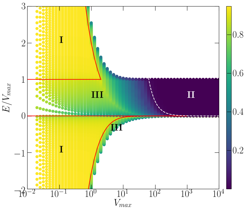
Figure 5: The entire phase diagram of the mosaic potential with $\kappa=2$. Localization is diagnosed by the fractal dimension. Red solid lines and the white dotted line mark mobility edges by Eq. (10) and Ref. Dwiputra and Zen (2022), respectively. Color represents the value of the fractal dimension. $L=2000$, $\kappa=2$.

Consequently, we have determined mobility edges separating weakly Wannier-Stark localized states from extended states. Here we complete the entire phase diagram of the mosaic system by referring to the previous work about strongly Wannier-Stark localized states Dwiputra and Zen (2022). It should be clearly pointed out that the Lyapunov exponent cannot distinguish between weakly and strongly Wannier-Stark localized states, due to $\gamma(E)>0$ for both two localized states. Alternatively, we utilize the fractal dimension to characterize different phases for mosaic potentials. As shown in Fig. 5, the red solid lines are the mobility edges obtained in the present work, while the white dashed line is the “mobility edge” in Ref. Dwiputra and Zen (2022). These two types of mobility edges divide the spectra into three regions: $D\approx 1$ for the extended region (I region), $D\approx 0$ for the strongly Wannier-Stark localized region (II region), and the remaining region is the weakly Wannier-Stark localized region (III region). It is worth mentioning that the recent work shows that, strictly speaking, disorder-free mobility edges do not exist, all states are Wannier-Stark localized states with the exception of $(\kappa-1)$-isolated extended states Longhi (2023). This conclusion is not contradictory to the present work, since we employ a finite-height Wannier-Stark ladder where $V_{max}$ does not depend on the size, while they use an infinite-height one with $V_{max}\propto L$. More explicitly, when $L\rightarrow\infty$, $V_{max}$ is finite in the present work, whereas $V_{max}\rightarrow\infty$ in Ref. Longhi (2023). These two types of potentials ($V_{max}$ is finite or infinite) can both be realized in experiments, corresponding to the weak and strong linear potentials Mendez et al. (1988); Voisin et al. (1988); Mendez and Bastard (1993), respectively. Crucially, our results show that mobility edges highly depend on $V_{max}$ and the system with a finite-height Wannier-Stark ladder is a good platform for the observation of disorder-free mobility edges.

Figure 6: The wave functions after time evolution $|\Psi(\tau)|^{2}$ in the left panels and the corresponding fidelities $f(\tau)$ in the right panels as a function of time $\tau$. In (a) and (d), the particle is at $j=L/2$ in the initial state, whereas it is at $j=L/2+1$ in (b), (c), (e), and (f). $V_{max}=10$ in (a), (b), (d), and (e), while $V_{max}=10^{3}$ in (c) and (f). $L=500$, $\kappa=2$. To indicate the wave functions clearly, we control the range of the color bar from 0.0 to 0.05 in the left panels.

To dynamically identify extended states, weakly Wannier-Stark localized states, and strongly Wannier-Stark localized states, we investigate the dynamical evolution $|\Psi(\tau)\rangle=e^{-iH\tau}|\Psi(0)\rangle$ of the initial state $|\Psi(0)\rangle$ and the fidelity $f=\left|\langle\Psi(\tau)|\Psi(0)\rangle\right|^{2}$. Firstly, we set $V_{max}=10$ for a weak mosaic potential. In Fig. 6 (a), the wave function spreads to the entire chain during time evolution when the energy of the initial state is in the extended region. On the contrary, Fig. 6 (b) shows that when the energy of the initial state is in the weakly Wannier-Stark localized region, the wave function oscillates periodically with time. This phenomenon is the well-known Bloch oscillation Bloch (1929), which is the typical dynamical characteristic of the Wannier-Stark localized states. The fidelities corresponding to the wave functions in Fig. 6 (a) and (b) manifest that $f(\tau)$ drops to zero after long-time evolution and the local information of the initial state is erased in Fig. 6 (d), whereas $f(\tau)$ periodically oscillates to preserve the local information in Fig. 6 (e). Secondly, we set $V_{max}=10^{3}$ for a strong mosaic potential to study the dynamical evolution of strongly Wannier-Stark localized states. In Fig. 6 (c), the wave function does not change obviously during time evolution, because the amplitude of the Bloch oscillation is suppressed. Correspondingly, in Fig. 6 (f) the fidelity keeps $f\approx 1.0$ and the local information is stored for any time.

V conclusion

In summary, we have studied the mobility edges in one-dimensional systems subjected to finite-height linear and mosaic potentials, respectively. In the present work, we take the Lyapunov exponent as the primary quantity to discriminate localization phenomena. By exploiting the property that the nearest-neighbor transfer matrices are approximately equal, we introduce a method to obtain the revised Lyapunov exponent, and exactly determine mobility edges separating weakly Wannier-Stark localized states from extended states in both cases. Especially, in the latter case, we demonstrate a richer phase diagram relative to the previous work, including an extended region, a weak Wannier-Stark localization region, and a strong Wannier-Stark localization region. As the height of the potential increases, the region of extended states is compressed and extended states only survive at $E\approx 0$ for high ladders. Furthermore, we also verify predicted mobility edges through the fractal dimension and demonstrate that the numerical results are reliable based on the size-effect analysis. These interesting features will bring new perspectives to a wide range of localization and disorder-free systems.