Scalable Algorithms for 2-Packing Sets on Arbitrary Graphs

Abstract

A 2-packing set for an undirected graph $G=(V,E)$ is a subset $\mathcal{S}\subset V$ such that any two vertices $v_{1},v_{2}\in\mathcal{S}$ have no common neighbors. Finding a 2-packing set of maximum cardinality is a NP-hard problem. We develop a new approach to solve this problem on arbitrary graphs using its close relation to the independent set problem. Thereby, our algorithm red2pack uses new data reduction rules specific to the 2-packing set problem as well as a graph transformation. Our experiments show that we outperform the state-of-the-art for arbitrary graphs with respect to solution quality and also are able to compute solutions multiple orders of magnitude faster than previously possible. For example, we are able to solve 63% of the graphs in the tested data set to optimality in less than a second while the competitor for arbitrary graphs can only solve 5% of these graphs to optimality even with a 10 hour time limit. Moreover, our approach can solve a wide range of large instances that have previously been unsolved.

1 Introduction

For a given undirected graph $G=(V,E)$ a 2-packing set is defined as a subset $\mathcal{S}\subseteq V$ of all vertices such that for each pair of distinct vertices $v_{1}\neq v_{2}\in\mathcal{S}$ the shortest path between $v_{1}$ and $v_{2}$ has at least length three. A maximum 2-packing set (M2S) is a 2-packing set with highest cardinality. A generalization of the maximum 2-packing set problem is the maximum $k$-packing set problem, where the shortest path length is bounded by $k$. For $k=1$ this results in the maximum independent set (MIS) problem. An important application for the maximum 2-packing set problem is given for example in distributed algorithms. In contrast to the independent set problem, which given a solution vertex only conflicts the direct neighborhood, the 2-packing set provides information about a larger area around the vertex. This is important for self-stabilizing algorithms [21, 22, 42, 46, 54, 53, 51]. In particular, computing large 2-packing sets can be used as a subroutine to ensure mutual exclusion of vertices with overlapping neighborhoods. An example is finding a minimal {$k$}-dominating function [21] which has various applications itself as presented by Gairing et al.[23]. Bacciu et al.[5] use large $k$-packing sets to develop a Downsampling approach for graph data. This is particularly useful for deep neural networks. Further, Soto et al.[29] show that the knowledge of the size of a maximum 2-packing set in special graphs can be used for error correcting codes and Hale et al.[30] indicate that large 2-packing sets can be used to model interference issues for frequency assignment. This can be done by looking at the frequency-constrained co-channel assignment problem. Here, the vertex set consists of locations of radio transmitters and two vertices share an edge if the frequencies are mutually perceptible. Now we want to assign a channel to as many radio transmitters as possible to conserve spectrum and to avoid interference issues vertices assigned the same channel must have a certain distance. For the distance two, this can be solved via finding a maximum 2-packing set in the corresponding graph. The maximum 2-packing set problem can be solved quite fast to optimality for small instances, however, since it is a NP-hard problem, the running time of exact algorithm grows exponentially with the size of the graph. One powerful technique for tackling $\mathbf{NP}$-hard graph problems is to use data reduction rules, which remove or contract local (hyper)graph structures, to reduce the input instance to an equivalent, smaller instance. Originally developed as a tool for parameterized algorithms [14], data reduction rules have been effective in practice for computing an (unweighted) maximum independent set [11, 33, 47] / minimum vertex cover [3], maximum clique [12, 55], and maximum $k$-plex [13, 32], as well as solving graph coloring [41, 55] and clique cover problems [25, 48], among others [2]. To the best of our knowledge, no data reduction rules have yet been investigated for the 2-packing set problem. The maximum 2-packing set problem can be solved with a graph transformation by expanding the 2 neighborhood and applying independent set solvers on the square graph. In recent years there was a lot of engineering yielding highly scalable solvers for maximum (weighted) independent set. However, graphs can get very dense if we directly compute the graph transformation which prohibits scalability. Thus problem specific data reductions are applied on the original problem instance first, and then we compute the expanded graph on which we solve the maximum independent set problem.

Our Results. Next to the new data reduction rules for the maximum 2-packing set problem, we also contribute a novel exact algorithm red2pack_b&r as well as a heuristic algorithm red2pack_heuristic. Both use these reductions to solve the maximum 2-packing set problem for arbitrary graphs on large scale. These algorithms work in three phases. First the data reductions are applied to the given graph resulting in a reduced instance. Afterwards, the resulting graph is transformed, such that a solution on the transformed graph for the MIS problem corresponds to a solution of the maximum 2-packing set problem for the original graph. The third phase of the algorithms consists of solving the MIS problem on the transformed graph. In this phase our two variants differ. For red2pack_b&r we use an exact solver, while we use a heuristic algorithm for red2pack_heuristic. Our experiments indicate that our algorithms outperform current state-of-the-art algorithms for arbitrary graphs both in terms of solution quality and running time. For instance, we can compute optimal solutions for 63% of our graphs in under a second, whereas the competing method for arbitrary graphs achieves this only for 5% of the graphs even with a 10-hour time frame. Lastly, our method solves many large instances that remained unsolved before.

2 Preliminaries

Let ${G=(V,E)}$ be an undirected graph with ${n=|V|}$ and ${m=|E|}$, where ${V=\{0,...,n-1\}}$. We extend this graph definition with further information about the 2-neighbors. Therefore, we define a graph $\mathcal{G}=(V,E,\mathcal{E})$ with the set of vertices $V$ and edges $E$ as before. With the set $\mathcal{E}$ we include additional edges connecting vertices that share a common neighbor, but are not directly connected. We only use the graph $\mathcal{G}$ when we emphasize the use of the additional edges $\mathcal{E}$, but all concepts introduced for the graph $G$ can be easily expanded for $\mathcal{G}$. The neighborhood $N(v)$ of a vertex $v\in V$ is defined as $N(v)=\{u\in V:(u,v)\in E\}$ and $N[v]=N(v)\cup\{v\}$. The notation is extended to a set of vertices $U\subseteq V$ with $N(U)=\cup_{u\in U}N(u)\setminus U$ and $N[U]=N(U)\cup U$. Analogue we define the 2-neighborhood as the neighborhood via edges in $\mathcal{E}$ of a vertex $v\in V$ as $N_{2}(v)=\{u\in V:(u,v)\in\mathcal{E}\}$ and $N_{2}[v]=N_{2}(v)\cup N[v]$. The notation is extended to a set of vertices $U\subseteq V$ with $N_{2}(U)=\cup_{u\in U}N_{2}(u)\setminus N[U]$ and $N_{2}[U]=N_{2}(U)\cup N[U]$. These notations are analogue extended for $k$-neighborhoods. We define the subset of edges in $\mathcal{E}$ connecting the vertices with a common neighbor $v$ by $\mathcal{E}(v)\coloneqq\{(x,y):x,y\in N_{2}(v)\ and\ (x,y)\notin E\}$. The degree of a vertex $v$ is the size of its neighborhood $\deg(v)=|N(v)|$. The 2-degree of a vertex is defined by the size of its 2-neighborhood $\textnormal{deg}^{2}(v)=|N_{2}(v)|$. The square graph $G^{2}=(V,E^{2})$ of a graph $G=(V,E)$ is defined as a graph with the same vertex set and an extended edge set. Here, an edge $(u,v)$ is added if the distance between $u$ and $v$ is at most 2. For ${0<k\in\mathbb{N}}$ a $k$-packing set is defined as a subset ${\mathcal{S}\subseteq V}$ of all vertices such that between each pair of vertices in $\mathcal{S}$ the shortest path contains at least $k+1$ edges. For $k=1$ we refer to the set as the independent set, where all vertices in $\mathcal{S}$ have to are non-adjacent. The main focus in this work lies on the case $k=2$, where all vertices in $\mathcal{S}$ must not have a common neighbor. A maximal 2-packing set is a 2-packing set $\mathcal{S}\subseteq V$ that can not be extended by any further vertex $v\in V$ without violating the 2-packing set conditions. The maximum 2-packing set problem is that of finding a 2-packing set with maximum cardinality. Analogue to the independence number $\alpha(G)$ for the maximum independent set, we define $\beta(G)$ as the size of the solution to the maximum 2-packing set problem for a given graph $G$.

In a path a 2-edge contributes 2 to its length. A 2-clique is as set of vertices in $\mathcal{G}$ such that they are pairwise connected by a path of at most length 2. A vertex $v$ is called 2-isolated if the vertices that are in its 2-neighborhood $N_{2}[v]$ form a 2-clique.

3 Related Work

3.1 2-Packing Set Algorithms

There are not many contributions to sequential algorithms for the 2-packing set problem on arbitrary graphs. Trejo-Sánchez et al.[49] are the first and as far as we know only authors to have proposed a sequential algorithm for connected arbitrary graphs. They developed a genetic algorithm for the M2S problem in which they use local improvements in each round of their algorithm and a penalty function. Ding et al.[16] propose a self-stabilizing algorithm with safe convergence in an arbitrary graph. The algorithm consists basically of two operations, namely entering the solution candidate and exiting the solution candidate for each vertex in the graph. If a vertex enters the solution its neighbors get locked so they can not enter the solution and cause a conflict. The decision to enter or exit the solution is based on the simple criteria to check whether a vertex causes a conflict or not. In general, most of the contributions to the 2-packing set problem on arbitrary graphs are in the context of distributed algorithms [21, 42, 46]. Further, there are some contributions to distributed algorithms for the M2S problem for special graphs. Flores-Lamas et al.[20] present a distributed algorithm that finds a maximal 2-packing set in an undirected non-geometric Halin graph in linear time. They use reduction rules by Eppstein [18] to determine a partition of the vertex set on which they base a coloring scheme to determine a maximal 2-packing set. However, the reduction of the graph is only used temporarily to compute the vertex partition and the coloring phase of the algorithm works on the original graph. Fernández-Zepeda et al.[50] present a distributed algorithm for a M2S in geometric outerplanar graphs. Mjelde [43] presents a self-stabilizing algorithm for the maximum $k$-packing set problem on tree graphs. Further, Mjelde [43] present a sequential algorithm for the M2S problem on tree graphs using dynamic programming. For special graphs there are also some non-distributed algorithms for the M2S problem [29, 19, 52]. Trejo-Sánchez et al.[52] present an approximation algorithm called Apx-2p + Imp2p using graph decompositions and LP-solvers. The approximation ratio is related to how the algorithm decomposes the input graph into smaller subgraphs which is inspired by Baker [7]. They also mention the possibility to solve the maximum 2-packing set problem by using a graph transformation to the square graph and apply independent set solver. However, this is not used for their algorithm. This equivalence was stated by Halldórsson et al.[31].

3.2 Independent Set Algorithms

Since our algorithms use independent set algorithms we also summarize closely related work on this topic. As exact approaches to this problem mainly use data reduction techniques we summarize heuristic approaches for the unweighted as well as for the weighted case because a lot of research happens in this area. A widely used technique are local search algorithms. The main idea behind it is to start from an initial solution and then to improve this solution by insertions or swaps. The algorithm of Andrade et al.[4] proved to be a successful algorithm in this area. The basic idea is to perform $(1,2)$-swaps, i.e. to delete one vertex from the solution and add two new vertices. Hence, the solution size increases by one. Other local search approaches proved to be successful too [44, 10, 40, 9]. Further, there are also contributions that combine local search algorithms with data reduction [39] and graph neural networks [38]. There are also reduction based heuristics for the MIS problem. Lamm et al.[34] present a branch-and-reduce approach combined with an evolutionary algorithm. Further, Gu et al.[28] use data reduction and a tie-breaking policy to apply data reductions repeatedly until they reach an empty graph.

3.3 Data Reduction Rules

Our algorithm uses data reductions in problem specific context as well as for solving the MIS problem on the transformed graph. Therefore, we summarize some related work on this topic with respect to the MIS problem as well. In recent years the branch-and-reduce paradigm has been shown to be an effective method to solve the maximum independent set problem to optimality as well as its complementary problem the minimum vertex cover [3]. By this paradigm we mean branching algorithms that use reduction rules to decrease the input size. Akiba and Iwata show that this approach yields good results in comparison to other exact approaches for minimum vertex cover problem and the maximum independent set problem [3]. Further, this approach is successfully used for the maximum weighted independent set problem. Lamm et al.[36] use this approach for an exact algorithm. Further, data reductions are also used for heuristics. Großmann et al.[27] use reduction rules in combination with an evolutionary approach for solving the maximum weighted independent set problem on huge sparse networks. Gao et al.[24] use inexact reduction rules by performing multiple rounds of a local search algorithm to determine vertices that are likely to be part of a solution to the MIS problem.

4 The Algorithm red2pack

Algorithm 1 High-level view of red2pack. Structure of both B&R and Heuristic.

  input graph ${\mathcal{G}=(V,E,\mathcal{E})}$

  output M2S

  procedure red2pack($\mathcal{G}$)

   $K\leftarrow$reduce($\mathcal{G}$)

   $K^{2}\leftarrow$transform($K$)

   MISsolve($K^{2}$)

We now give an overview of the components of our algorithm. The idea of our approach is to build a square graph on which a maximum independent set is equivalent to a maximum 2-packing set on the original graph (see Theorem 4.11). On this transformed graph, we apply well studied maximum independent set solvers to find optimal solutions. During the transformation we increase the number of edges in the graph. Since this results in more dense graphs, this approach becomes quite slow and necessitates a substantial amount of memory. To alleviate this issue, we add a preprocessing step. There, we apply new problem specific data reductions exhaustively to the graph to obtain a kernel $\mathcal{K}$. We then apply the transformation on $\mathcal{K}$, resulting in a significantly smaller square graph. On this a maximum independent set solver is applied to obtain a (optimum) solution. In the end, the solution is transformed to a (optimum) solution to the input instance. Overall, this results in the algorithm red2pack (see Algorithm 1). In the following we introduce our new data reductions, then present the used graph transformation and finally give details about the maximum independent set solvers used.

4.1 Data Reduction Rules

To reduce the problem size especially for large instances exact data reductions are very useful tools. In general our reductions allow us to identify vertices as (1) part of a solution to the maximum 2-packing set problem (included) and (2) as non-solution vertices (excluded). The reductions are applied exhaustively in a predefined order. If a reduction is successful, we start again by applying the first reduction.

We denote the reduced graph by $\mathcal{G}^{\prime}$ and $\beta(\mathcal{G})$ is the solution size to the maximum 2-packing set problem for the given graph $\mathcal{G}$. For the 2-packing set problem we first introduce the two core data reductions in the following.

Reduction 4.1 (Domination).

Let ${v,u\in V}$ be vertices such that $N_{2}[v]\subseteq N_{2}[u]$. Then, there is some M2S of $\mathcal{G}$ that does not contain $u$. In particular, the graph is reduced to $\mathcal{G}^{\prime}=\mathcal{G}[V\setminus\{u\}]$ and $\beta(\mathcal{G})=\beta(\mathcal{G}^{\prime})$.

Proof.

Let ${v,u\in V}$ and $N_{2}[v]\subseteq N_{2}[u]$. Further assume $\mathcal{S}$ is a M2S in $\mathcal{G}$ containing $u$. Since $N_{2}[v]\subseteq N_{2}[u]$, it holds for all vertices $x\in N_{2}[v]\setminus\{u\}$ that $x\notin\mathcal{S}$. We define $\mathcal{S}^{\prime}=(\mathcal{S}\setminus\{u\})\cup\{v\}$ and it holds $|\mathcal{S}|=|\mathcal{S}^{\prime}|$. Further, $\mathcal{S}^{\prime}$ is still a valid 2-packing set since there is no vertex in $N_{2}[v]\setminus\{v\}$ that is also element of $\mathcal{S}^{\prime}$. By construction $\mathcal{S}^{\prime}$ has the same size and therefore is a equivalent solution to M2S not containing $u$. ∎

Reduction 4.2 (Clique).

Let $v\in V$ be 2-isolated in $\mathcal{G}$. Then, $v$ is in some M2S of $\mathcal{G}$. Therefore, we can include $v$ and exclude $N_{2}[v]$. Resulting in $\mathcal{G}^{\prime}=\mathcal{G}[V\setminus N_{2}[v]]$ and $\beta(\mathcal{G})=\beta(\mathcal{G}^{\prime})+1$.

Proof.

Let $\mathcal{S}\subseteq V$ be a M2S in $\mathcal{G}$. Since $v$ is 2-isolated at least one vertex $w\in N_{2}[v]$ is contained in $\mathcal{S}$, otherwise $\mathcal{S}$ is not maximal. Assume $w\neq v$ and $N_{2}[v]$ forms a 2-clique, it holds ${u\notin\mathcal{S}}$ for all ${u\in N_{2}[v]\setminus\{w\}}$. Additionally, since $v$ is 2-isolated ${N_{2}[v]\subseteq N_{2}[w]}$. Therefore, we can always build a new solution $\mathcal{S}^{\prime}=(\mathcal{S}\setminus\{w\})\cup\{v\}$ of the same size containing $v$. This way we can always construct an equivalent or better solution when including $v$ and therefore the vertex $v$ is in some M2S of $\mathcal{G}$. Reducing the graph by including $v$ results in $\beta(G)=1+\beta(\mathcal{G}[V\setminus N_{2}[v]])$. ∎

These two reductions require knowledge about the 2-neighborhood as a prerequisite. Computing the 2-neighborhood of a vertex $v$ can become quite large and verifying these conditions is computationally expensive. Hence, we have sought out different special cases where it suffices to consider only the direct neighborhood and impose a constraint on the degree of the 2-neighborhood, which we maintain. Adding the following special cases to the core data reductions yields our elaborated data reductions. The following lemma helps us to show that these special cases are instances of the more general case.

Lemma 4.1.

Let $u,v\in V$ be neighbors in $\mathcal{G}$ with $N[v]\subseteq N[u]$ such that $\textnormal{deg}^{2}(v)+\deg(v)\leq\deg(u)$. Then, $N_{2}(v)=N[u]\setminus N[v]$, i.e. all 2-neighbors of the vertex $v$, are also neighbors of the vertex $u$.

Proof 4.2.

Let $u,v\in V$ be neighbors with $N[v]\subseteq N[u]$ such that $\textnormal{deg}^{2}(v)+\deg(v)\leq\deg(u)$. By definition of the 2-neighborhood we know that $N[u]\setminus N[v]\subseteq N_{2}(v)$. Therefore, we know that $\deg(u)+1-(\deg(v)+1)\leq\textnormal{deg}^{2}(v)$ which is equivalent to $\deg(u)\leq\textnormal{deg}^{2}(v)+\deg(v)$. Because of the assumption $\textnormal{deg}^{2}(v)+\deg(v)\leq\deg(u)$, there has to hold an equality and therefore the sets have to be the same $N_{2}(v)=N[u]\setminus N[v]$.

Reduction 4.3 (Degree Zero Reduction).

Let $v\in V$ be a degree zero vertex. Furthermore, let $\textnormal{deg}^{2}(v)\leq 1$. Then, $v$ is in some M2S of $\mathcal{G}$. Therefore, vertex $v$ can be included and the 2-neighborhood of $v$ excluded. Resulting in $\mathcal{G}^{\prime}=\mathcal{G}[V\setminus N_{2}[v]]$ and $\beta(\mathcal{G})=\beta(\mathcal{G}^{\prime})+1$.

Proof 4.3.

Let ${v\in V}$ be a vertex with ${\deg(v)=0}$ and $\textnormal{deg}^{2}(v)\leq 1$. For the case of $\textnormal{deg}^{2}(v)=0$ there is no conflict and $v$ can be included in the solution. In the case of $\textnormal{deg}^{2}(v)=1$, let the 2-neighbor of $v$ be $u\in N_{2}(v)$. Assume $u$ is part of the solution $\mathcal{S}$. Then, we can create a new solution by $\mathcal{S}^{\prime}=\mathcal{S}\setminus\{u\}\cup\{v\}$ of same size. This way we always find a M2S including $v$.

Figure 1: Original graph on the left reduced to the graph on the right. Due to clarity reasons, we only display the necessary edges from $\mathcal{E}$ (dashed) regarding the 2-neighborhood information.

(a) Domination Reduction: $N_{2}[u]$ is colored with orange, $N_{2}[v]$ with blue. The vertex $u$ dominates $v$ and therefore $u$ can be excluded.

(b) Twin Reduction: The neighbors $u,w\in V$ of $v$ are twins. We can include $v$ into the solution and exclude its 2-neighborhood $N_{2}[v]$.

Reduction 4.4 (Degree Zero Triangle).

Let $v\in V$ be a degree zero vertex. Furthermore, let $\textnormal{deg}^{2}(v)=2$ with 2-neighbors $N_{2}(v)=\{u,w\}$ that are also adjacent via an edge or 2-edge $u\in N_{2}[w]$. Then, $v$ is in some M2S of $\mathcal{G}$. Therefore, vertex $v$ can be included and the 2-neighborhood of $v$ excluded. This results in $\mathcal{G}^{\prime}=\mathcal{G}[V\setminus N_{2}[v]]$ and $\beta(\mathcal{G})=\beta(\mathcal{G}^{\prime})+1$.

Proof 4.4.

Let ${v\in V}$ be a vertex of ${\deg(v)=0}$ and $\{u,w\}=N_{2}(v)$ its 2-neighbors adjacent via an edge or 2-edge $u\in N_{2}[w]$. Vertices $u$ and $w$ dominate vertex $v$ and can therefore be excluded by Reduction 4.1. Now Reduction 4.3 is applicable and vertex $v$ can be included into the solution.

Reduction 4.5 (Degree One).

Let $v\in V$ be a degree one vertex with ${N(v)=\{u\}}$. Furthermore, let $\textnormal{deg}^{2}(v)\leq\deg(u)-1$. Then, $v$ is in some M2S of $\mathcal{G}$. Therefore, vertex $v$ can be included and the 2-neighborhood of $v$ excluded. This results in $\mathcal{G}^{\prime}=\mathcal{G}[V\setminus N_{2}[v]]$ and $\beta(\mathcal{G})=\beta(\mathcal{G}^{\prime})+1$.

Proof 4.5.

Let ${v\in V}$ be a vertex with ${\deg(v)=1}$ and ${N(v)=\{u\}}$ with $\textnormal{deg}^{2}(v)\leq\deg(u)-1$. We can apply Lemma 4.1 and it holds that $N_{2}[v]=N[u]$. Therefore, this represents a special case of the 2-clique and Reduction 4.2 can be applied.

Reduction 4.6 (Degree Two V-Shape).

Let ${v\in V}$ be a vertex of ${\deg(v)=2}$ with $N(v)=\{u,w\}$ and $\textnormal{deg}^{2}(v)=0$. Then, $v$ is in some M2S of $\mathcal{G}$. The graph is reduced to $\mathcal{G}^{\prime}=\mathcal{G}[V\setminus N_{2}[v]]$ and $\beta(\mathcal{G})=\beta(\mathcal{G}^{\prime})+1$.

Proof 4.6.

Let the above stated assumptions hold. Then, $N_{2}[v]\subseteq N_{2}[u]$ and $N_{2}[v]\subseteq N_{2}[w]$ the vertices $w$ and $u$ can be excluded by Reduction 4.1. Since $|N_{2}(v)|=0$, vertex $v$ can safely be included.

Reduction 4.7 (Degree Two Triangle).

Let ${v\in V}$ be a vertex of ${\deg(v)=2}$ with $N(v)=\{u,w\}$ and $2=\deg(u)=\deg(w)$. Furthermore, let $\textnormal{deg}^{2}(v)=0$. Then $v$ is in some M2S of $\mathcal{G}$. The graph is reduced to $\mathcal{G}^{\prime}=\mathcal{G}[V\setminus N_{2}[v]]$ and $\beta(\mathcal{G})=\beta(\mathcal{G}^{\prime})+1$.

Proof 4.7.

Let the vertices $v,u,w\in V$ all have degree two and $N(v)=\{u,w\}$ and $\textnormal{deg}^{2}(v)=0$. In this case, the vertices $u$, $v$ and $w$ form a triangle. Since $N_{2}[v]\subseteq N_{2}[u]$ and $N_{2}[v]\subseteq N_{2}[w]$ the vertices $w$ and $u$ can be excluded by Reduction 4.1. Since $|N_{2}(v)|=0$, vertex $v$ can safely be included.

Reduction 4.8 (Degree Two 4-Cycle).

Let ${u,v,w,x\in V}$ be vertices with $\deg(v)=\deg(u)=\deg(w)=2$, $N(v)=\{u,w\}$ and $N_{2}(v)=\{x\}$. Furthermore, let $x\in N(u)$ and $x\in N(w)$. Then, the vertices build a 4-cycle and $v$ is in some M2S of $\mathcal{G}$. The graph is reduced to $\mathcal{G}^{\prime}=\mathcal{G}[V\setminus N_{2}[v]]$ and $\beta(\mathcal{G})=\beta(\mathcal{G}^{\prime})+1$.

Proof 4.8.

Assuming the above stated assumptions such that the vertices $u$, $v$, $w$ and the one 2-neighbor $x\in N_{2}(v)$ form a 4-cycle. It holds that $N_{2}[v]=\{u,v,w,x\}\subseteq N_{2}[u]$, therefore, we can exclude the vertex $u$ by Reduction 4.1. Analogue, we can exclude vertex $w$. Assume $x$ is part of a M2S $\mathcal{S}$. Then, we can create a new solution $\mathcal{S}^{\prime}=\mathcal{S}\setminus\{x\}\cup\{v\}$ of same size. This way we always find a M2S including $v$.

Reduction 4.9 (Fast Domination).

Let ${v,u\in V}$ be vertices such that $N[v]\subseteq N[u]$ and $\textnormal{deg}^{2}(v)+\deg(v)\leq\deg(u)$. Then, there is some M2S of $\mathcal{G}$ without $u$. The graph is reduced to $\mathcal{G}^{\prime}=\mathcal{G}[V\setminus\{u\}]$ and $\beta(\mathcal{G})=\beta(\mathcal{G}^{\prime})$.

Proof 4.9.

Let ${v,u\in V}$ and $N[v]\subseteq N[u]$ with $\textnormal{deg}^{2}(v)+\deg(v)\leq\deg(u)$. Using Lemma 4.1 we know $N_{2}(v)=N[u]\setminus N[v]$. It holds that $N_{2}[v]\subseteq N_{2}[u]$ and Reduction 4.1 is applicable.

Reduction 4.10 (Twin).

Let ${v\in V}$ be a vertex of degree ${\deg(v)=2}$ and ${u,w\in V}$ be its neighbors with $N(u)=N(w)$. Furthermore, let $\textnormal{deg}^{2}(v)\leq\deg(u)-1$. Then, $u$ and $w$ are twins and $v$ is in some M2S of $\mathcal{G}$. We reduce $\mathcal{G}^{\prime}=\mathcal{G}[V\setminus N_{2}[v]]$ and $\beta(\mathcal{G})=\beta(\mathcal{G}^{\prime})+1$.

Proof 4.10.

Let ${v\in V}$ be a vertex with ${\deg(v)=2}$ and ${u,w\in V}$ be its neighbors with $N(u)=N(w)$. The additional assumption $\textnormal{deg}^{2}(v)\leq\deg(u)-1=\deg(w)-1$ ensures that all 2-neighbors of $v$ are connected to the vertices $u$ and $w$. Analogue to Lemma 4.1 but for the neighborhood of $u$ and $v$ not a subset. This way $\mathcal{G}[N_{2}[v]]$ forms a 2-clique, and therefore, this reduction is a special case of Reduction 4.2.

4.1.1 Miscellaneous

We now motivate the importance of the edge set $\mathcal{E}$. When a vertex $v$ is included by a reduction, its 2-neighborhood has to be excluded to obtain a valid maximum 2-packing set. In Figure 2(a) we perform Reduction 4.5 on the original graph $G$ without the separate 2-neighbor edges $\mathcal{E}$. Here, we do not get a valid solution since the information, that $n_{1},\ n_{2}$ and $n_{3}$ are in the same 2-neighborhood is lost. When we apply the reduction on $\mathcal{G}$ we do not lose connecting edges in $\mathcal{E}(w)$ of an excluded vertex $w$. This is illustrated in Figure 2(b).

Figure 2: Demonstration of the vital role of retaining 2-neighborhood information for non-reduced vertices in maintaining a valid solution to the M2S problem. Reduced vertices and edges are light gray shaded. Green vertices are included, red vertices are excluded from the solution.

(a) Degree One Reduction without $\mathcal{E}$ loosing the 2-neighborhood information yielding an invalid solution.

(b) Degree One Reduction with necessary 2-neighborhood information via $\mathcal{E}$ resulting in a valid M2S.

4.1.2 Data Structure

Our reductions operate on a dynamic graph data structure based on adjacency arrays representing undirected edges by two directed edges. Internally, we separate edges and 2-edges with two adjacency arrays. A key observation of our reductions is that we often do not need to know the 2-neighborhood to exclude a vertex. This can be seen for example in the Degree One Reduction applied to a vertex $v$ with its neighbor $u$. Then, we do not need to consider $N_{2}(u)$. In general, we only compute and then store the 2-neighborhood of a vertex $v$ on demand.

This also leads to less effort, compared to initially constructing the 2-neighborhood for the whole graph, when reducing the graph. When a vertex $u$ is removed from the graph, we delete every edge and 2-edge pointing to it. Removing all incoming edges can take $\mathcal{O}(\Delta^{4})$ time where $\Delta$ is the highest degree in the graph. With the on-demand technique we can also reduce the amount of computations there, i.e. if the 2-neighborhood of a vertex $v$ is not computed in advance there are potentially less edges that are deleted in this step.

4.2 Graph Transformation

Figure 3: The graph ${\mathcal{G}=(V,E,\mathcal{E})}$ on the left with edges in $\mathcal{E}$ marked as dashed lines. This graph is transformed to ${G^{2}=(V,E^{2})}$ on the right. The green vertices present the M2S (left) and the MIS (right).

After we applied all data reduction rules exhaustively, i.e. there is no data reduction rule that can still be applied, we begin the transformation of the reduced graph to the square graph.

For this process we start with a graph ${G=(V,E)}$ and add all edges in $\mathcal{E}$ as regular edges. The resulting set of edges is referred to as $E^{2}=E\cup\mathcal{E}$, and the transformed square graph is denoted as ${G^{2}=(V,E^{2})}$. This way the set of regular edges is extended to also contain edges connecting pairs of vertices $u,w\in V$ that have a common neighbor. Since $E\cap\mathcal{E}=\emptyset$ we do not add parallel edges. Figure 3 illustrates of the square graph.

Theorem 4.11.

Let ${G=(V,E)}$ be a given graph and ${G^{2}=(V,E^{2})}$ the transformed graph. Then, an optimal solution to the maximum independent set problem on $G^{2}$ is an optimal solution for the maximum 2-packing set problem on the original graph $G$ [31].

4.3 MIS Solver

We have chosen to use the solver by Lamm et al.[37] since it is a state-of-the-art exact solver for the independent set problem. However, it is also possible to integrate any other exact solver for the maximum independent set problem. Note that we did not chose the branch and reduce solver for the unweighted problem [35], since with it we are restricted to smaller graphs. While our focus is on optimal solution, we also combine our solver with OnlineMIS [15], resulting in our heuristic red2pack_heuristic. For a briefly description of the main components of the solver by Lamm et al.[37] and the solver by Dahlum et al.[15] we refer to our technical report [8].

5 Experimental Evaluation

Methodology. We implemented our algorithm using C++17. The code is compiled using g++ version 12.2 and full optimizations turned on (-O3). We used a machine equipped with a AMD EPYC 7702P (64 cores) processor and 1 TB RAM running Ubuntu 20.04.1. We ran all of our experiments with four different random seeds and report geometric mean values unless mentioned otherwise. We set the time limit for all algorithms to 10h. If a solver exceeded a memory threshold of 100 GB during execution we stop the solver and mark this with m.o.. If the algorithm terminated due to the time limit, we mark it with t.o. in the results. In both cases we report the best solution found until this point. To compare different algorithms, we use performance profiles [17], which depict the relationship between the objective function size or running time of each algorithm and the corresponding values produced or consumed by the algorithms. Specifically, the y-axis represents the fraction of instances where the objective function is less than or equal to $\tau$ times the best objective function value, denoted as $\#\{\textnormal{objective}\leq\tau\ast\textnormal{best}\}/\#G$. Here, “objective“ refers to the result obtained by an algorithm on an instance, and “best" corresponds to the best result among all the algorithms shown in the plot. #$G$ is the number of graphs in the data set. When considering the running time, the y-axis displays the fraction of instances where the time taken by an algorithm is less than or equal to $\tau$ times the time taken by the fastest algorithm on that instance, denoted as $\#\{\textnormal{t}\leq\tau\ast\textnormal{ fastest}\}/\#\textnormal{instances}$. Here, “t“ represents the time taken by an algorithm on an instance, and “fastest" refers to the time taken by the fastest algorithm on that specific instance. The parameter $\tau$, which is greater than or equal to 1, is plotted on the x-axis. Each algorithm’s performance profile yields a non-decreasing, piecewise constant function.

Table 1: Effect of graph transformation: Arithmetic mean percentage of number of vertices $\tilde{n}=n(K^{2})/n(G)$ and edges $\tilde{m}=m(K^{2})/m(G)$ in transformed graph after different reduction variants. Since 2pack does not apply reductions, this column represents the square graphs $G^{2}$. For detailed results, see Table 3.

	2pack		core		elaborated
	$\tilde{n}$[%]	$\tilde{m}$[%]	$\tilde{n}$[%]	$\tilde{m}$[%]	$\tilde{n}$[%]	$\tilde{m}$[%]
planar	100	212,11	99,91	211,67	99,91	211,67
social (s)	100	3 154,00	14,48	70,25	14,48	70,25
social (l)	100	4 327,38	17,12	274,56	17,12	274,58
overall	100	2 564,50	43,84	185,49	43,84	185,50

Overview/Competing Algorithms. We perform a wide range of experiments. First we perform experiments to investigate the influence of the data reduction rules in Section 5.1. Therefore, we define three configurations for our reductions. The first variant is called 2pack and does not include any of our proposed reductions. Then, in core we only use the Domination and Clique Reduction. For the last variant elaborated we apply the full set of all special case reductions as well as the Domination and Clique Reduction. The order for reductions in core is [4.2, 4.1] while elaborated uses [4.3, 4.4, 4.5, 4.7, 4.8, 4.6, 4.10, 4.9, 4.1, 4.2]. Note that we did not experiment with different orderings for the reductions since Großmann et al.show in [27, 26] that for the MWIS problem an intuitive ordering worked best and small changes do not effect the solution quality and running time by a lot. We then compare our algorithms against the state-of-the-art for the problem in Section 5.2. In particular, we compare against the genetic algorithm gen2pack by Trejo-Sánchez et al.[49] as well as the Apx-2p + Imp2p algorithm by Trejo-Sánchez et al.[52] which only works for planar graphs. We use two configurations of Apx-2p + Imp2p. The configurations differ in the parameter $h$ which specifies, the number of vertices in the subgraphs. With increasing $h$ the solution quality improves, but the slower the algorithm performs. We chose the default configuration with $h=50$ and $h=100$ to improve the solution and give a fairer comparison with our 10 hour time limit. We could not perform experiments with Maximum-2-Pack-Cactus since the code is not available [1] and the data in the paper itself is presented such that a direct comparison is not possible.

Data Sets. We collected a wide range of instances for our experiments different sources. First, we use a set of social networks in our benchmark which are typically used to benchmark recent independent set algorithms. More precisely, we use forty social networks from [45] and [6]. We split this class up into two sets of twenty graphs each by the number of vertices in the graphs, i.e. we put graphs with less than 50 000 vertices in small social subset and the others in large social. We only added instances for the benchmark were the number of edges did not exceed 32-bit when constructing the two-neighborhood with the 2pack algorithm. Note that this only happened for large graphs and not for any of the instances that were used in previous experiments for the maximum 2-packing set problem. When comparing against the other algorithms, we also include 20 cactus graphs from [19] as well as a random selection of 1 050 Erdös–Rényi graphs from [49]. To be able to compare against Apx-2p + Imp2p, we also include planar graphs from [52]. For an overview of the graph properties we refer to [8].

5.1 Impact of Data Reductions

We now investigate the effectiveness of the data reductions. To do so, we use the three reduction configurations for the algorithm red2pack_b&r. To evaluate the effectiveness we do not investigate the influence on Erdös–Rényi as well as Cactus graphs, as they are already very small. We compare the impact on the size of the square kernels as well as solution quality and running time. Details are presented in Tables 3 and 4. We summarize these results in Table 1 and Figure 4.

First, we look at the effectiveness of our reductions on the size of the square kernels $K^{2}$. When applying the graph transformation on the original input, i.e. without applying any reduction (2pack), the resulting instance has the same amount of vertices and on average 25,65$\cdot m(G)$ edges, whereas core and elaborated both yield on average $0.44\cdot|V|$ vertices and $1.86\cdot|E|$ edges. Thus, our data reductions help to decrease the size of the transformed graph by more than a factor of ten on average. The approaches core and elaborated compute overall the same kernel sizes. However, on five large social instances elaborated computes smaller kernels, but only with a very small difference. On planar graphs our reduction rules, as expected, are not working good since they have mesh-like structure. The number of vertices in the kernel is only reduced by 0,1% compared to the original graph. All together we are able to reduce 15 out of 60 instances to an empty kernel and thereby solve them solely by our data-reductions. Hence, we conclude that the reductions are highly effective in reducing the graph size and especially reduce the size for social networks.

Figure 4: Solution quality (left) and running time (right) for red2pack_b&r on planar and social graphs comparing our different reduction variants.

Regarding solution quality overall our variant elaborated is performing only slightly better compared to the other variants. Especially on the small social and planar graphs hardly a difference can be seen. When considering large social graphs, however, we can find no instance, on which 2pack outperforms core or elaborated. Overall, we achieve an improvement through elaborated on this graph class of 0,05% compared to 2pack and core. The instance with the largest difference in solution quality is road_usa. Here, elaborated achieves an improvement of 0,93% over the other two strategies. On the instance amazon-2008 elaborated performs worse compared to core. On this, the solution quality of core is improved by 0,10% compared to the solution of elaborated. For all of the 6 instances, on which elaborated was outperformed by 2pack the improvement over elaborated is always smaller than 0,01%.

Figure 4 also show that using our different data reduction rules as a preprocessing step (core and elaborated) especially improves the running time compared to 2pack. Here, we see that in general our reductions are improving the performance and our approach elaborated works best. In the detailed results in Table 4 we see that especially for large social graphs elaborated yields a speed up of 2,7 compared to 2pack. On planar graphs, where our reductions are not effective in reducing the initial input size, the performance is very similar for all our variants.

Conclusion: We conclude that for all examined criteria, which are the size of the square kernel as well as solution quality and running time, our variant elaborated performs best. Hence, we choose the elaborated reduction variant in the following state-of-the-art comparisons for both red2pack_b&r and red2pack_heuristic.

5.2 Comparison against State-of-the-Art

We now compare our algorithms red2pack_b&r and red2pack_heuristic using our best reduction variant elaborated, against other state-of-the-art algorithms which are gen2pack by Trejo-Sánchez et al.[49] as well as two configurations of Apx-2p + Imp2p by Trejo-Sánchez et al.[52].

gen2pack: For the comparison against gen2pack we only use cactus graphs and Erdös–Rényi (erdos) networks, i.e. the instances used in their paper, as gen2pack is not able to solve any of the other, larger graphs within the given time limit. This can be explained by the initial computations containing matrix multiplication used in gen2pack. This does not finish during the 10 hours limit, so that the algorithm could not compute any solution at all. Detailed per instance results for this comparison can be found in Table 6.

Table 2: Summary comparison of state-of-the-art. Detailed results are presented in Tables 6 to 5. Geometric mean over different graph classes of solution size $|S|$ and time $t$ to find it. Best results are emphasized in bold. Apx-2P + Im2p with $h=100$ is omitted as not all planar instances where solved within the time limit.

			Apx-2p + Im2p		red2pack		red2pack
	gen2pack		($h=50$)		b&r		heuristic
Class	$|S|$	$t$ [s]	$|S|$	$t$ [s]	$|S|$	$t$ [s]	$|S|$	$t$ [s]
cactus	104	1 384 007,11	-		137	4,26	137	7,30
erdos	8	21 679,67	-		9	0,31	9	0,53
planar	-		110 009	255,04	92 135	10,41	110 095	31 706,65
social (s)	-		-		159	11,32	159	13,53
social (l)	-		-		30 066	6 442,49	30 756	26 377,56

In Figure 5 we give performance profiles for running time and solution quality. In Table 2 we give the geometric mean running times and solution qualities for these results. Our algorithm red2pack_b&r as well as red2pack_heuristic find overall the optimal solution in the classes cactus and erdos within a few milliseconds. Our algorithms dominate gen2pack in terms of both solution quality as well as running time. Especially the differences in running time are very large. On all graphs our two algorithms are multiple orders of magnitude faster than gen2pack. It can only find optimal solutions for 6 out of these 40 graphs, see Table 6. On these two graph classes both our algorithms always compute the optimum solution quality which results in an average solution quality improvement of more than 20% and a speedup of more than $10^{5}$. Among all instances under consideration, on Erdos37-2 gen2pack needed the least amount of time to compute an optimum solution. For this instance we achieve with red2pack_b&r a speed up of more than 300 000 and more than 350 000 with red2pack_heuristic. The instance on which gen2pack needs the most time is cac1000. On this instance, red2pack_b&r and red2pack_heuristic again have similar speedups in the range of $10^{5}$ over gen2pack and an improvement in solution quality of roughly 32%. Considering the overall data set, our approach red2pack_b&r can solve 63 out of 100 graphs to optimality within less than one second and 71 within the 10 hour time limit and 100GB restriction. For instances that we could not solve to optimality due to experimental restrictions, we give the solution found until this point, see Tables 4 and 6.

In Table 5 we compare red2pack_b&r and red2pack_heuristic on social graphs, which are not solvable with the competitors. On these instances we are able to achieve an average improvement in solution quality of around 1% with red2pack_heuristic compared to red2pack_b&r. Especially for large graphs, where our exact solver meets the memory threshold, our heuristic variant is able to outperform the results of red2pack_b&r.

Apx-2p + Imp2p: Since our reductions do not perform well on planar graphs, we are not able to solve them to optimality with red2pack_b&r and exceed the memory threshold quite fast. Overall, the solution quality we achieve with red2pack_b&r for the planar graphs is 84% of the solution quality that the competitor Apx-2p + Imp2p ($h=50$) computes, but we only use 4% of its time needed. With red2pack_heuristic, on the other hand, we outperform Apx-2p + Imp2p ($h=50$) on all but one instance regarding solution quality, see Table 6. We achieve an average solution quality which is on par, i.e. our improvement over the competitors results by 0,08%. Note that the authors experimentally show in [52] that the computed 2-packing set by Apx-2p + Imp2p is already at least 99% of the optimum solution. However, on those instances our algorithms needs roughly two orders of magnitude more running time than Apx-2p + Imp2p ($h=50$). Apx-2p + Imp2p with $h=100$ compared to $h=50$ can improve all but one solution, however the running time increase is up to multiple orders of magnitude and some instances where not solved within the 10 hour time limit. red2pack_heuristic is able to find better solutions than Apx-2p + Imp2p ($h=100$) on 9 out of 20 instances. Again the differences in solution quality are very small. Detailed results for these experiments are given in Table 6 and Figure 5 (right). The competitor gen2pack for general graphs is unable to solve any of these instances which is why we omitted it in the corresponding tables and performance profiles.

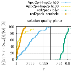
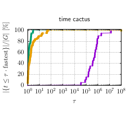
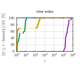
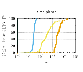
Figure 5: State of the art comparison on solution quality (top) and running time (bottom) for different graph classes. For planar graphs (right) the competitor gen2pack is not able to solve the instances. To this end we add the algorithm Apx-2p + Imp2p with $h=50$ and $h=100$ as well as red2pack_heuristic for comparison.

Conclusion: We conclude that on all instances we are able to outperform the competitor gen2pack for arbitrary graphs in both solution quality and running time by multiple orders of magnitude. Moreover, we can solve a wide range of instances to optimality that previously have been unsolvable. When comparing against algorithms specialized on planar graphs, we presented two options: one that is by more than a factor of 24 times faster with lower solution quality and one that is on par in terms of solution quality, but slower, compared to both configurations of the state-of-the-art specialized solver for planar graphs.

6 Conclusion and Future Work

This work introduces novel data reduction rules to solve the maximum 2-packing set problem as well as proposes a new exact algorithm red2pack_b&r that uses these reductions to exactly solve the maximum 2-packing set problem on large-scale arbitrary graphs. Additionally, a new heuristic algorithm red2pack_heuristic is introduced that works similar. Both of the algorithms red2pack_b&r and red2pack_heuristic work in three phases. First the new data reduction rules are applied to the given input resulting in a reduced instance. Following the reduction phase, the resulting graph is transformed, such that a solution on the transformed graph for the maximum independent set problem corresponds to a solution of the maximum 2-packing set problem for the original graph. The third phase of the algorithms consists of solving the maximum independent set problem on the transformed graph. Our tests indicate that our algorithms outperform the previous best algorithm for arbitrary graphs both in terms of solution quality and running time on all instances. For instance, we can compute optimal solutions for 63% of our graphs in under a second, whereas the competing method for arbitrary graphs achieves this only for 5% of the graphs even with a 10-hour time frame. Furthermore, our method successfully solves many large instances that remained unsolved before. Lastly, our algorithm can compete with a specialized solver on planar instances in terms of solution size and computes near optimum solutions. Our code is publicly available under https://github.com/KarlsruheMIS/red2pack.

In future work, we want to find more reduction rules, especially for mesh-like graphs. We are also interested in the weighted 2-packing set problem as well as the $k$-packing set problem for larger values of $k$ and find independent motifs in graphs via hypergraphs matching algorithms.

Appendix A Reduction and Transformation Details

Table 3: Percentage of remaining vertices and edges for different reduction variants after transformation. Bolt numbers indicate the best results, gray background marks empty kernels.

				red2pack_b&r		red2pack_b&r
		2pack		core		elaborated
Class	Graphs	$n(K^{2})/n\leavevmode\nobreak\ [\%]$	$m(K^{2})/m\leavevmode\nobreak\ [\%]$	$n(K^{2})/n\leavevmode\nobreak\ [\%]$	$m(K^{2})/m\leavevmode\nobreak\ [\%]$	$n(K^{2})/n\leavevmode\nobreak\ [\%]$	$m(K^{2})/m\leavevmode\nobreak\ [\%]$
social (s)	PGPgiantcompo	100,00	873,91	0,00	0,00	0,00	0,00
	adjnoun	100,00	725,18	0,00	0,00	0,00	0,00
	as-22july06	100,00	22 941,92	0,00	0,00	0,00	0,00
	celegans_metabolic	100,00	2 239,56	0,00	0,00	0,00	0,00
	celegansneural	100,00	1 123,00	30,64	98,46	30,64	98,46
	chesapeake	100,00	407,65	0,00	0,00	0,00	0,00
	cond-mat	100,00	678,06	0,00	0,00	0,00	0,00
	dolphins	100,00	381,76	0,00	0,00	0,00	0,00
	email	100,00	1 114,57	0,00	0,00	0,00	0,00
	email-EuAll	100,00	16 882,03	0,14	0,07	0,14	0,07
	football	100,00	476,18	100,00	476,18	100,00	476,18
	hep-th	100,00	535,64	0,00	0,00	0,00	0,00
	jazz	100,00	488,48	6,57	1,79	6,57	1,79
	lesmis	100,00	491,73	0,00	0,00	0,00	0,00
	netscience	100,00	245,15	0,00	0,00	0,00	0,00
	p2p-Gnutella04	100,00	1 227,55	74,85	638,90	74,85	638,90
	polbooks	100,00	453,97	50,48	105,67	50,48	105,67
	power	100,00	343,18	2,83	4,88	2,83	4,88
	soc-Slashdot0902	100,00	8 678,73	24,12	79,04	24,12	79,07
	wordassociation-2011	100,00	2 771,82	0,00	0,00	0,00	0,00
social (l)	G_n_pin_pout	100,00	1 088,81	99,35	1 075,38	99,35	1 075,38
	amazon-2008	100,00	901,89	11,27	35,64	11,27	35,66
	astro-ph	100,00	1 469,69	0,02	0,00	0,02	0,00
	caidaRouterLevel	100,00	1 843,47	0,67	0,67	0,67	0,67
	citationCiteseer	100,00	2 980,56	0,08	0,03	0,08	0,03
	cnr-2000	100,00	20 072,23	4,32	378,64	4,34	378,94
	coAuthorsCiteseer	100,00	1 005,95	0,00	0,00	0,00	0,00
	coAuthorsDBLP	100,00	1 262,80	0,01	0,01	0,01	0,01
	coPapersCiteseer	100,00	823,64	0,01	0,00	0,01	0,00
	coPapersDBLP	100,00	1 572,96	0,01	0,00	0,01	0,00
	cond-mat-2003	100,00	1 149,60	0,03	0,02	0,03	0,02
	cond-mat-2005	100,00	1 467,49	0,00	0,00	0,00	0,00
	enron	100,00	9 684,16	0,00	0,00	0,00	0,00
	loc-brightkite_edges	100,00	4 026,75	0,00	0,00	0,00	0,00
	loc-gowalla_edges	100,00	25 177,85	0,03	0,01	0,03	0,01
	preferentialAttachment	100,00	3 386,36	100,00	3 386,36	100,00	3 386,36
	road_central	100,00	261,10	13,55	35,31	13,55	35,31
	road_usa	100,00	261,17	13,46	35,13	13,46	35,13
	smallworld	100,00	550,88	99,20	543,05	99,20	543,05
	web-Google	100,00	7 560,20	0,41	0,87	0,42	0,94
planar	outP500_1	100,00	213,51	99,94	213,20	99,94	213,20
	outP500_2	100,00	212,22	99,93	211,87	99,93	211,87
	outP1000_1	100,00	212,19	99,85	211,53	99,85	211,53
	outP1000_2	100,00	211,92	99,87	211,29	99,87	211,29
	outP1500_1	100,00	211,86	99,95	211,60	99,95	211,60
	outP1500_2	100,00	211,97	99,94	211,68	99,94	211,68
	outP2000_1	100,00	211,93	99,93	211,58	99,93	211,58
	outP2000_2	100,00	211,97	99,91	211,53	99,91	211,53
	outP2500_1	100,00	212,10	99,86	211,45	99,86	211,45
	outP2500_2	100,00	212,14	99,91	211,72	99,91	211,72
	outP3000_1	100,00	212,12	99,89	211,62	99,89	211,62
	outP3000_2	100,00	212,11	99,88	211,56	99,88	211,56
	outP3500_1	100,00	212,13	99,88	211,55	99,88	211,55
	outP3500_2	100,00	212,00	99,91	211,58	99,91	211,58
	outP4000_1	100,00	212,01	99,90	211,55	99,90	211,55
	outP4000_2	100,00	211,99	99,92	211,61	99,92	211,61
	outP4500_1	100,00	212,04	99,88	211,50	99,88	211,50
	outP4500_2	100,00	212,05	99,92	211,69	99,92	211,69
	outP5000_1	100,00	212,06	99,91	211,64	99,91	211,64
	outP5000_2	100,00	211,96	99,92	211,56	99,92	211,56
overall	planar and social	100,00	2 564,50	43,84	185,49	43,84	185,50

Table 4: Solution size $|S|$ and time $t$ needed to find it. The time $t_{p}$ is the time needed to prove the optimality. Bolt numbers indicate best results, gray background optimally solved instances.

					red2pack_b&r			red2pack_b&r
		2pack			core			elaborated
Class	Graphs	$|S|$	$t$ [s]	$t_{p}$ [s]	$|S|$	$t$ [s]	$t_{p}$ [s]	$|S|$	$t$ [s]	$t_{p}$ [s]
social (s)	PGPgiantcompo	2 708	0,02	0,02	2 708	0,01	0,01	2 708	0,01	0,01
	adjnoun	18	<0,01	<0,01	18	<0,01	<0,01	18	<0,01	<0,01
	as-22july06	2 026	4,26	4,26	2 026	0,95	0,96	2 026	1,74	1,74
	celegans_metabolic	29	0,01	0,01	29	<0,01	<0,01	29	<0,01	<0,01
	celegansneural	14	0,06	0,06	14	0,05	0,06	14	0,06	0,06
	chesapeake	3	<0,01	<0,01	3	<0,01	<0,01	3	<0,01	<0,01
	cond-mat	3 391	0,03	0,03	3 391	0,02	0,02	3 391	0,02	0,02
	dolphins	13	<0,01	<0,01	13	<0,01	<0,01	13	<0,01	<0,01
	email	209	0,01	0,01	209	0,01	0,01	209	<0,01	<0,01
	email-EuAll	696	2,74	2,74	696	1,83	1,83	696	1,56	1,56
	football	7	1,36	1,39	7	1,36	1,39	7	1,35	1,39
	hep-th	2 611	0,01	0,01	2 611	0,01	0,01	2 611	<0,01	0,01
	jazz	13	<0,01	<0,01	13	<0,01	<0,01	13	<0,01	<0,01
	lesmis	10	<0,01	<0,01	10	<0,01	<0,01	10	<0,01	<0,01
	netscience	477	<0,01	<0,01	477	<0,01	<0,01	477	<0,01	<0,01
	p2p-Gnutella04	825	0,35	m.o.	825	0,35	m.o.	825	0,33	m.o.
	polbooks	12	<0,01	<0,01	12	<0,01	<0,01	12	<0,01	<0,01
	power	1 465	<0,01	<0,01	1 465	<0,01	<0,01	1 465	<0,01	<0,01
	soc-Slashdot0902	3 280	27,43	m.o.	3 282	19,77	m.o.	3 282	3,53	m.o.
	wordassociation-2011	2 473	0,28	0,28	2 473	0,04	0,04	2 473	0,02	0,02
overall	social (s)	159	0,02	-	159	0,01	-	159	0,01	-
social (l)	G_n_pin_pout	7 116	8,18	m.o.	7 116	8,46	m.o.	7 116	8,64	m.o.
	amazon-2008	106 533	71,17	m.o.	106 558	68,58	m.o.	106 556	70,55	m.o.
	astro-ph	2 926	0,28	0,28	2 926	0,09	0,09	2 926	0,05	0,05
	caidaRouterLevel	40 138	3,11	3,21	40 138	1,49	1,51	40 138	0,73	0,74
	citationCiteseer	43 238	10,39	10,39	43 238	2,51	2,51	43 238	1,72	1,72
	cnr-2000	21 897	1 031,59	m.o.	21 896	986,12	m.o.	21 897	1 030,06	m.o.
	coAuthorsCiteseer	33 167	1,22	1,22	33 167	0,56	0,56	33 167	0,40	0,40
	coAuthorsDBLP	43 960	2,37	2,37	43 960	0,73	0,73	43 960	0,67	0,67
	coPapersCiteseer	26 001	47,88	47,88	26 001	33,65	33,65	26 001	14,70	14,70
	coPapersDBLP	35 529	121,92	121,92	35 529	90,89	90,89	35 529	18,21	18,21
	cond-mat-2003	5 374	0,17	0,17	5 374	0,08	0,08	5 374	0,06	0,06
	cond-mat-2005	6 505	0,39	0,39	6 505	0,16	0,16	6 505	0,10	0,10
	enron	4 090	11,21	11,21	4 090	1,42	1,43	4 090	1,25	1,26
	loc-brightkite_edges	12 940	2,18	2,18	12 940	0,40	0,41	12 940	0,18	0,19
	loc-gowalla_edges	41 590	350,55	351,65	41 590	76,80	76,82	41 590	70,81	70,83
	preferentialAttachment	6 397	15,35	m.o.	6 397	15,54	m.o.	6 397	15,95	m.o.
	road_central	4 289 510	2 566,67	m.o.	4 289 578	2 299,59	m.o.	4 289 639	2 441,79	m.o.
	road_usa	7 296 706	3 697,55	m.o.	7 296 913	3 043,52	m.o.	7 297 028	3 733,19	m.o.
	smallworld	6 872	5,19	m.o.	6 872	5,36	m.o.	6 872	5,38	m.o.
	web-Google	30 296	62,47	63,40	30 296	34,77	34,83	30 296	68,16	68,22
overall	social (l)	30 065	16,58	-	30 066	8,38	-	30 066	6,44	-
planar	outP500_1	19 140	1,64	m.o.	19 140	1,75	m.o.	19 140	1,77	m.o.
	outP500_2	21 894	2,16	m.o.	21 894	2,27	m.o.	21 894	2,25	m.o.
	outP1000_1	43 855	4,28	m.o.	43 855	4,73	m.o.	43 855	4,76	m.o.
	outP1000_2	45 418	4,10	m.o.	45 418	4,53	m.o.	45 418	4,65	m.o.
	outP1500_1	69 368	6,33	m.o.	69 368	6,59	m.o.	69 368	6,71	m.o.
	outP1500_2	68 571	6,45	m.o.	68 571	6,69	m.o.	68 571	6,84	m.o.
	outP2000_1	90 550	8,26	m.o.	90 550	8,60	m.o.	90 550	8,76	m.o.
	outP2000_2	90 507	8,44	m.o.	90 505	9,08	m.o.	90 505	9,18	m.o.
	outP2500_1	113 643	10,83	m.o.	113 635	11,72	m.o.	113 635	11,99	m.o.
	outP2500_2	113 073	10,73	m.o.	113 066	11,30	m.o.	113 066	11,55	m.o.
	outP3000_1	135 658	13,22	m.o.	135 659	14,57	m.o.	135 659	14,95	m.o.
	outP3000_2	136 101	13,45	m.o.	136 101	15,11	m.o.	136 101	15,67	m.o.
	outP3500_1	161 706	13,85	m.o.	161 709	15,14	m.o.	161 709	15,42	m.o.
	outP3500_2	162 533	14,23	m.o.	162 528	15,73	m.o.	162 528	16,17	m.o.
	outP4000_1	178 655	17,55	m.o.	178 671	18,77	m.o.	178 671	19,36	m.o.
	outP4000_2	178 862	17,64	m.o.	178 858	19,12	m.o.	178 858	19,69	m.o.
	outP4500_1	198 172	21,96	m.o.	198 176	23,59	m.o.	198 176	24,17	m.o.
	outP4500_2	198 440	21,81	m.o.	198 440	22,78	m.o.	198 440	23,26	m.o.
	outP5000_1	226 396	21,77	m.o.	226 395	24,31	m.o.	226 395	25,15	m.o.
	outP5000_2	33 663	13,39	m.o.	33 663	15,23	m.o.	33 663	15,84	m.o.
overall	planar	92 135	9,43	-	92 135	10,19	-	92 135	10,41	-
overall	social and planar	7 604	1,50	-	7 604	1,04	-	7 604	0,91	-

Appendix B Detailed State-of-the-Art Comparison

Table 5: Solution size $|S|$ and time $t$ needed to find it. The time $t_{p}$ is the time needed to prove the optimality. Bolt numbers indicate best results in comparison. Gray background marks optimally solved instances. No competitor is able to solve these instances.

		red2pack			red2pack
		b&r			heuristic
Class	Graphs	$|S|$	$t$ [ms]	$t_{p}$ [ms]	$|S|$	$t$ [ms]
social (s)	PGPgiantcompo	2 708	8,34	8,74	2 708	8,31
	adjnoun	18	0,43	0,48	18	0,43
	as-22july06	2 026	1 737,58	1 739,08	2 026	1 774,51
	celegans_metabolic	29	4,77	4,84	29	4,81
	celegansneural	14	55,94	58,29	14	57,74
	chesapeake	3	0,13	0,18	3	0,13
	cond-mat	3 391	16,42	17,09	3 391	16,92
	dolphins	13	0,12	0,16	13	0,11
	email	209	3,44	3,58	209	3,49
	email-EuAll	696	1 561,44	1 561,44	696	1 463,69
	football	7	1 351,83	1 388,30	7	223,50
	hep-th	2 611	4,77	5,07	2 611	4,85
	jazz	13	2,18	2,18	13	7,12
	lesmis	10	0,16	0,20	10	0,16
	netscience	477	1,24	1,38	477	1,31
	p2p-Gnutella04	825	332,37	m.o.	837	1 695,12
	polbooks	12	1,97	2,62	12	5,57
	power	1 465	3,67	3,92	1 465	17,06
	soc-Slashdot0902	3 282	3 532,80	m.o.	3 288	3 314,43
	wordassociation-2011	2 473	22,04	22,50	2 473	22,43
overall	social (s)	159	11,32	-	159	13,53
social (l)	G_n_pin_pout	7 116	8 640,57	m.o.	7 970	1 706 124,41
	amazon-2008	106 556	70 549,59	m.o.	107 165	15 503 659,26
	astro-ph	2 926	51,34	51,34	2 926	50,86
	caidaRouterLevel	40 138	732,05	742,47	40 138	799,62
	citationCiteseer	43 238	1 719,69	1 719,69	43 238	1 658,55
	cnr-2000	21 897	1 030 063,00	m.o.	21 898	931 990,73
	coAuthorsCiteseer	33 167	402,64	402,64	33 167	370,94
	coAuthorsDBLP	43 960	672,32	672,32	43 960	630,44
	coPapersCiteseer	26 001	14 702,18	14 702,18	26 001	14 979,70
	coPapersDBLP	35 529	18 210,66	18 210,66	35 529	17 866,85
	cond-mat-2003	5 374	59,71	59,71	5 374	61,45
	cond-mat-2005	6 505	99,69	101,85	6 505	100,22
	enron	4 090	1 254,90	1 258,90	4 090	1 233,50
	loc-brightkite_edges	12 940	182,96	185,44	12 940	182,93
	loc-gowalla_edges	41 590	70 812,67	70 825,69	41 590	71 102,93
	preferentialAttachment	6 397	15 947,59	m.o.	7 034	2 608 316,99
	road_central	4 289 639	2 441 793,42	m.o.	4 499 839	35 841 231,91
	road_usa	7 297 028	3 733 186,22	m.o.	7 647 882	35 970 721,50
	smallworld	6 872	5 379,45	m.o.	7 946	11 329 895,89
	web-Google	30 296	68 160,24	68 222,93	30 296	67 864,36
overall	social (l)	30 066	6 442,49	-	30 756	26 377,56
overall		2 184	270,05	-	2 210	597,37

Table 6: Solution size $|S|$ and time $t$ needed to find it. The time $t_{p}$ is the time needed to prove the optimality. Bolt numbers indicate best results in comparison. Gray background marks optimally solved instances.

				red2pack			red2pack
		gen2pack		b&r			heuristic
Class	Graphs	$|S|$	$t$ [ms]	$|S|$	$t$ [ms]	$t_{p}$ [ms]	$|S|$	$t$ [ms]
cactus	cac50	15	25 291,12	17	0,05	0,09	17	0,05
	cac100	28	85 674,26	31	0,09	0,14	31	0,09
	cac150	42	181 973,07	49	0,31	0,31	49	13,49
	cac200	55	313 878,10	65	10,27	10,70	65	14,47
	cac250	68	484 267,30	82	0,69	0,79	82	0,25
	cac300	80	712 988,40	100	0,83	0,83	100	13,07
	cac350	92	963 595,66	116	12,89	13,35	116	13,66
	cac400	103	1 230 210,54	133	14,58	15,26	133	30,00
	cac450	114	1 574 182,46	148	12,22	12,66	148	13,70
	cac500	126	1 987 312,28	166	23,73	25,24	166	17,65
	cac550	136	2 389 870,11	179	15,61	15,98	179	18,59
	cac600	146	2 779 427,76	199	0,24	0,30	199	0,23
	cac650	158	3 328 099,16	214	28,90	29,19	214	58,65
	cac700	165	3 859 839,95	232	7,68	7,72	232	8,82
	cac750	172	4 477 170,66	250	11,58	11,58	250	19,19
	cac800	184	5 088 716,64	264	18,26	18,87	264	19,84
	cac850	196	5 648 560,45	282	26,46	27,04	282	26,27
	cac900	205	6 490 942,35	300	10,92	11,35	300	29,14
	cac950	214	7 281 058,31	315	10,18	10,18	315	17,17
	cac1000	223	8 084 805,96	332	17,02	17,46	332	58,03
overall	cactus	104	1 384 007,11	137	4,26	4,66	137	7,30
erdos	Erdos37-2	9	21 118,31	9	0,07	0,11	9	0,06
	Erdos37-16	8	21 119,42	9	1,13	1,25	9	2,31
	Erdos37-23	9	21 104,45	10	0,09	0,13	10	0,09
	Erdos37-44	7	21 318,79	7	0,99	1,19	7	0,14
	Erdos37-45	10	21 328,35	11	0,09	0,13	11	0,08
	Erdos38-2	9	21 706,27	9	0,07	0,11	9	0,07
	Erdos38-14	8	21 915,50	9	0,59	0,68	9	2,50
	Erdos38-18	6	21 969,36	7	1,25	1,35	7	4,59
	Erdos38-46	8	21 927,82	9	1,05	1,19	9	14,31
	Erdos38-48	8	21 643,77	9	0,96	1,17	9	1,30
	Erdos39-14	9	22 997,65	9	0,16	0,16	9	0,08
	Erdos39-22	10	22 626,53	11	0,06	0,10	11	0,06
	Erdos39-25	8	23 005,90	8	1,30	1,69	8	0,48
	Erdos39-29	9	22 800,22	10	0,07	0,12	10	0,07
	Erdos39-44	8	22 758,11	9	0,11	0,15	9	0,10
	Erdos40-0	9	23 138,60	10	0,18	0,18	10	1,79
	Erdos40-4	8	19 244,44	9	0,26	0,26	9	1,21
	Erdos40-8	7	19 161,29	8	1,87	2,02	8	12,74
	Erdos40-10	10	23 474,02	10	0,22	0,22	10	1,04
	Erdos40-43	8	19 918,83	9	1,07	1,18	9	3,51
overall	erdos	8	21 679,67	9	0,31	0,38	9	0,53

		Apx-2p + Im2p		Apx-2p + Im2p		red2pack		red2pack
		($h=100$)		($h=50$)		b&r		heuristic
Class	Graphs	$|S|$	$t$ [s]	$|S|$	$t$ [s]	$|S|$	$t$ [s]	$|S|$	$t$ [s]
planar	outP500_1	20 333	97,51	20 327	22,99	19 140	1,77	20 332	26 166,03
	outP500_2	24 187	1 978,02	24 144	58,42	21 894	2,25	24 181	12 631,72
	outP1000_1	48 575	1 066,37	48 472	145,79	43 855	4,76	48 567	29 215,74
	outP1000_2	49 429	692,06	49 430	111,35	45 418	4,65	49 416	28 336,12
	outP1500_1	74 232	794,47	74 170	166,89	69 368	6,71	74 292	31 577,14
	outP1500_2	73 901	2 638,12	73 813	161,62	68 571	6,84	73 922	31 015,92
	outP2000_1	-	t.o.	98 519	333,63	90 550	8,76	98 555	32 735,67
	outP2000_2	98 643	2 062,41	98 558	251,90	90 505	9,18	98 669	33 103,01
	outP2500_1	122 826	1 092,08	122 761	233,20	113 635	11,99	122 831	34 384,01
	outP2500_2	122 322	4 897,24	122 275	319,30	113 066	11,55	122 282	34 018,53
	outP3000_1	146 748	1 739,13	146 622	258,05	135 659	14,95	146 696	35 371,22
	outP3000_2	147 544	1 633,60	147 360	341,67	136 101	15,67	147 522	35 483,06
	outP3500_1	171 303	14 025,36	171 127	490,08	161 709	15,42	171 264	34 414,78
	outP3500_2	-	t.o.	172 720	351,27	162 528	16,17	172 956	35 585,91
	outP4000_1	-	t.o.	196 172	490,55	178 671	19,36	196 189	35 262,82
	outP4000_2	196 218	19 284,45	196 076	540,26	178 858	19,69	196 243	35 367,19
	outP4500_1	220 799	4 932,77	220 677	505,56	198 176	24,17	220 737	35 650,42
	outP4500_2	221 406	11 015,21	221 283	503,34	198 440	23,26	221 345	35 643,68
	outP5000_1	244 641	12 413,34	244 350	595,94	226 395	25,15	244 548	35 605,20
	outP5000_2	245 031	6 309,16	245 038	603,84	33 663	15,84	245 223	35 789,86
overall	planar	-	-	110 009	255,04	92 135	10,41	110 095	31 706,65

References

- [1] Personal Communication with A. Lamas. 2023.
- [2] Faisal N. Abu-Khzam, Sebastian Lamm, Matthias Mnich, Alexander Noe, Christian Schulz, and Darren Strash. Recent advances in practical data reduction. In Hannah Bast, Claudius Korzen, Ulrich Meyer, and Manuel Penschuck, editors, Algorithms for Big Data: DFG Priority Program 1736, pages 97–133. Springer Nature Switzerland, Cham, 2022. doi:10.1007/978-3-031-21534-6_6.
- [3] T. Akiba and Y. Iwata. Branch-and-reduce exponential/FPT algorithms in practice: A case study of vertex cover. Theoretical Computer Science, 609, Part 1:211–225, 2016. doi:10.1016/j.tcs.2015.09.023.
- [4] Diogo Vieira Andrade, Mauricio G. C. Resende, and Renato Fonseca F. Werneck. Fast local search for the maximum independent set problem. J. Heuristics, 18(4):525–547, 2012. doi:10.1007/s10732-012-9196-4.
- [5] Davide Bacciu, Alessio Conte, and Francesco Landolfi. Generalizing downsampling from regular data to graphs, 2022. arXiv:2208.03523.
- [6] David A. Bader, Andrea Kappes, Henning Meyerhenke, Peter Sanders, Christian Schulz, and Dorothea Wagner. Benchmarking for graph clustering and partitioning. In Reda Alhajj and Jon G. Rokne, editors, Encyclopedia of Social Network Analysis and Mining, 2nd Edition. Springer, 2018. doi:10.1007/978-1-4939-7131-2\_23.
- [7] Brenda S. Baker. Approximation algorithms for np-complete problems on planar graphs. J. ACM, 41(1):153–180, jan 1994. doi:10.1145/174644.174650.
- [8] Jannick Borowitz, Ernestine Großmann, Christian Schulz, and Dominik Schweisgut. Finding optimal 2-packing sets on arbitrary graphs at scale. CoRR, abs/2308.15515, 2023. URL: https://doi.org/10.48550/arXiv.2308.15515, arXiv:2308.15515, doi:10.48550/ARXIV.2308.15515.
- [9] Shaowei Cai. Balance between complexity and quality: Local search for minimum vertex cover in massive graphs. In Qiang Yang and Michael J. Wooldridge, editors, Proceedings of the Twenty-Fourth International Joint Conference on Artificial Intelligence, IJCAI 2015, Buenos Aires, Argentina, July 25-31, 2015, pages 747–753. AAAI Press, 2015. URL: http://ijcai.org/Abstract/15/111.
- [10] Shaowei Cai, Wenying Hou, Jinkun Lin, and Yuanjie Li. Improving local search for minimum weight vertex cover by dynamic strategies. In Jérôme Lang, editor, Proceedings of the Twenty-Seventh International Joint Conference on Artificial Intelligence, IJCAI 2018, July 13-19, 2018, Stockholm, Sweden, pages 1412–1418. ijcai.org, 2018. doi:10.24963/ijcai.2018/196.
- [11] L. Chang, W. Li, and W. Zhang. Computing a near-maximum independent set in linear time by reducing-peeling. In Proc. of the 2017 ACM Intl. Conf. on Management of Data, pages 1181–1196. ACM, 2017.
- [12] Lijun Chang. Efficient maximum clique computation and enumeration over large sparse graphs. VLDB J., 29(5):999–1022, 2020. doi:10.1007/s00778-020-00602-z.
- [13] Alessio Conte, Donatella Firmani, Maurizio Patrignani, and Riccardo Torlone. A meta-algorithm for finding large -plexes. Knowl. Inf. Syst., 63(7):1745–1769, 2021. doi:10.1007/s10115-021-01570-8.
- [14] Marek Cygan, Fedor V Fomin, Łukasz Kowalik, Daniel Lokshtanov, Dániel Marx, Marcin Pilipczuk, Michał Pilipczuk, and Saket Saurabh. Parameterized algorithms, volume 4. Springer, 2015. doi:10.1007/978-3-319-21275-3.
- [15] Jakob Dahlum, Sebastian Lamm, Peter Sanders, Christian Schulz, Darren Strash, and Renato F. Werneck. Accelerating local search for the maximum independent set problem. In 15th International Symposium on Experimental Algorithms SEA, volume 9685 of Lecture Notes in Computer Science, pages 118–133. Springer, 2016. URL: https://doi.org/10.1007/978-3-319-38851-9_9.
- [16] Yihua Ding, James Z Wang, and Pradip K Srimani. Self-stabilizing algorithm for maximal 2-packing with safe convergence in an arbitrary graph. In 2014 IEEE international parallel & distributed processing symposium workshops, pages 747–754. IEEE, 2014.
- [17] Elizabeth D Dolan and Jorge J Moré. Benchmarking optimization software with performance profiles. Mathematical programming, 91(2):201–213, 2002. doi:10.1007/s101070100263.
- [18] David Eppstein. Simple recognition of halin graphs and their generalizations. J. Graph Algorithms Appl., 20(2):323–346, 2016. doi:10.7155/jgaa.00395.
- [19] Alejandro Flores-Lamas, José Alberto Fernández-Zepeda, and Joel Antonio Trejo-Sánchez. Algorithm to find a maximum 2-packing set in a cactus. Theoretical Computer Science, 725:31–51, 2018.
- [20] Alejandro Flores-Lamas, José Alberto Fernández-Zepeda, and Joel Antonio Trejo-Sánchez. A distributed algorithm for a maximal 2-packing set in halin graphs. Journal of Parallel and Distributed Computing, 142:62–76, 2020.
- [21] Martin Gairing, Robert M Geist, Stephen T Hedetniemi, and Petter Kristiansen. A self-stabilizing algorithm for maximal 2-packing. Nordic Journal of Computing, 11:1–11, 2004.
- [22] Martin Gairing, Wayne Goddard, Stephen T Hedetniemi, Petter Kristiansen, and Alice A McRae. Distance-two information in self-stabilizing algorithms. Parallel Processing Letters, 14(03n04):387–398, 2004.
- [23] Martin Gairing, Stephen T. Hedetniemi, Petter Kristiansen, and Alice A. McRae. Self-stabilizing algorithms for {k}-domination. In Shing-Tsaan Huang and Ted Herman, editors, Self-Stabilizing Systems, pages 49–60, Berlin, Heidelberg, 2003. Springer Berlin Heidelberg.
- [24] Wanru Gao, Tobias Friedrich, Timo Kötzing, and Frank Neumann. Scaling up local search for minimum vertex cover in large graphs by parallel kernelization. In Wei Peng, Damminda Alahakoon, and Xiaodong Li, editors, AI 2017: Advances in Artificial Intelligence - 30th Australasian Joint Conference, Melbourne, VIC, Australia, August 19-20, 2017, Proceedings, volume 10400 of Lecture Notes in Computer Science, pages 131–143. Springer, 2017. doi:10.1007/978-3-319-63004-5\_11.
- [25] Jens Gramm, Jiong Guo, Falk Hüffner, and Rolf Niedermeier. Data reduction and exact algorithms for clique cover. ACM J. Exp. Algorithmics, 13, feb 2009. doi:10.1145/1412228.1412236.
- [26] Ernestine Großmann, Sebastian Lamm, Christian Schulz, and Darren Strash. Finding near-optimal weight independent sets at scale. CoRR, abs/2208.13645, 2022. arXiv:2208.13645, doi:10.48550/arXiv.2208.13645.
- [27] Ernestine Großmann, Sebastian Lamm, Christian Schulz, and Darren Strash. Finding near-optimal weight independent sets at scale. In Sara Silva and Luís Paquete, editors, Proceedings of the Genetic and Evolutionary Computation Conference, GECCO 2023, Lisbon, Portugal, July 15-19, 2023, pages 293–302. ACM, 2023. doi:10.1145/3583131.3590353.
- [28] Jiewei Gu, Weiguo Zheng, Yuzheng Cai, and Peng Peng. Towards computing a near-maximum weighted independent set on massive graphs. In Feida Zhu, Beng Chin Ooi, and Chunyan Miao, editors, KDD ’21: The 27th ACM SIGKDD Conference on Knowledge Discovery and Data Mining, Virtual Event, Singapore, August 14-18, 2021, pages 467–477. ACMoeuristic, 2021. doi:10.1145/3447548.3467232.
- [29] J.M. Gómez Soto, J. Leaños, L.M. Ríos-Castro, and L.M. Rivera. The packing number of the double vertex graph of the path graph. Discrete Applied Mathematics, 247:327–340, 2018. URL: https://www.sciencedirect.com/science/article/pii/S0166218X18301938, doi:https://doi.org/10.1016/j.dam.2018.03.085.
- [30] W.K. Hale. Frequency assignment: Theory and applications. Proceedings of the IEEE, 68(12):1497–1514, 1980.
- [31] Magnús M. Halldórsson, Jan Kratochvíl, and Jan Arne Telle. Independent sets with domination constraints. In Kim Guldstrand Larsen, Sven Skyum, and Glynn Winskel, editors, Automata, Languages and Programming, 25th International Colloquium, ICALP’98, Aalborg, Denmark, July 13-17, 1998, Proceedings, volume 1443 of Lecture Notes in Computer Science, pages 176–187. Springer, 1998. doi:10.1007/BFb0055051.
- [32] Hua Jiang, Dongming Zhu, Zhichao Xie, Shaowen Yao, and Zhang-Hua Fu. A new upper bound based on vertex partitioning for the maximum -plex problem. In Zhi-Hua Zhou, editor, Proceedings of the Thirtieth International Joint Conference on Artificial Intelligence, IJCAI-21, pages 1689–1696. International Joint Conferences on Artificial Intelligence Organization, 8 2021. Main Track. doi:10.24963/ijcai.2021/233.
- [33] Sebastian Lamm, Peter Sanders, Christian Schulz, Darren Strash, and Renato F. Werneck. Finding near-optimal independent sets at scale. J. of Heuristics, 23(4):207–229, Aug 2017. doi:10.1007/s10732-017-9337-x.
- [34] Sebastian Lamm, Peter Sanders, Christian Schulz, Darren Strash, and Renato F. Werneck. Finding near-optimal independent sets at scale. J. Heuristics, 23(4):207–229, 2017. doi:10.1007/s10732-017-9337-x.
- [35] Sebastian Lamm, Peter Sanders, Christian Schulz, Darren Strash, and Renato F. Werneck. Finding near-optimal independent sets at scale. Journal of Heuristics, 23(4):207–229, 2017. doi:10.1007/s10732-017-9337-x.
- [36] Sebastian Lamm, Christian Schulz, Darren Strash, Robert Williger, and Huashuo Zhang. Exactly solving the maximum weight independent set problem on large real-world graphs. In Stephen G. Kobourov and Henning Meyerhenke, editors, Proceedings of the Twenty-First Workshop on Algorithm Engineering and Experiments, ALENEX 2019, San Diego, CA, USA, January 7-8, 2019, pages 144–158. SIAM, 2019. doi:10.1137/1.9781611975499.12.
- [37] Sebastian Lamm, Christian Schulz, Darren Strash, Robert Williger, and Huashuo Zhang. Exactly solving the maximum weight independent set problem on large real-world graphs. In 2019 Proceedings of the Twenty-First Workshop on Algorithm Engineering and Experiments (ALENEX), pages 144–158. SIAM, 2019. doi:10.1137/1.9781611975499.12.
- [38] Kenneth Langedal, Johannes Langguth, Fredrik Manne, and Daniel Thilo Schroeder. Efficient minimum weight vertex cover heuristics using graph neural networks. In Christian Schulz and Bora Uçar, editors, 20th International Symposium on Experimental Algorithms, SEA 2022, July 25-27, 2022, Heidelberg, Germany, volume 233 of LIPIcs, pages 12:1–12:17. Schloss Dagstuhl - Leibniz-Zentrum für Informatik, 2022. doi:10.4230/LIPIcs.SEA.2022.12.
- [39] Ruizhi Li, Shuli Hu, Shaowei Cai, Jian Gao, Yiyuan Wang, and Minghao Yin. Numwvc: A novel local search for minimum weighted vertex cover problem. J. Oper. Res. Soc., 71(9):1498–1509, 2020. doi:10.1080/01605682.2019.1621218.
- [40] Yuanjie Li, Shaowei Cai, and Wenying Hou. An efficient local search algorithm for minimum weighted vertex cover on massive graphs. In Yuhui Shi, Kay Chen Tan, Mengjie Zhang, Ke Tang, Xiaodong Li, Qingfu Zhang, Ying Tan, Martin Middendorf, and Yaochu Jin, editors, Simulated Evolution and Learning - 11th International Conference, SEAL 2017, Shenzhen, China, November 10-13, 2017, Proceedings, volume 10593 of Lecture Notes in Computer Science, pages 145–157. Springer, 2017. doi:10.1007/978-3-319-68759-9\_13.
- [41] Jinkun Lin, Shaowei Cai, Chuan Luo, and Kaile Su. A reduction based method for coloring very large graphs. In Proceedings of the Twenty-Sixth International Joint Conference on Artificial Intelligence, IJCAI-17, pages 517–523, 2017. doi:10.24963/ijcai.2017/73.
- [42] Fredrik Manne and Morten Mjelde. A memory efficient self-stabilizing algorithm for maximal k-packing. In Stabilization, Safety, and Security of Distributed Systems: 8th International Symposium, SSS 2006, Dallas, TX, USA, November 17-19, 2006. Proceedings 8, pages 428–439. Springer, 2006.
- [43] Morten Mjedle. -packing and -domination on tree graphs. Master’s thesis, University of Bergen, 2004.
- [44] Bruno C. S. Nogueira, Rian G. S. Pinheiro, and Anand Subramanian. A hybrid iterated local search heuristic for the maximum weight independent set problem. Optim. Lett., 12(3):567–583, 2018. doi:10.1007/s11590-017-1128-7.
- [45] Ryan A. Rossi and Nesreen K. Ahmed. The network data repository with interactive graph analytics and visualization. In AAAI, 2015. URL: https://networkrepository.com.
- [46] Zhengnan Shi. A self-stabilizing algorithm to maximal 2-packing with improved complexity. Information Processing Letters, 112(13):525–531, 2012.
- [47] Darren Strash. On the power of simple reductions for the maximum independent set problem. In Intl. Computing and Combinatorics Conf., pages 345–356. Springer, 2016.
- [48] Darren Strash and Louise Thompson. Effective Data Reduction for the Vertex Clique Cover Problem, pages 41–53. SIAM, 2022. doi:10.1137/1.9781611977042.4.
- [49] Joel Antonio Trejo-Sánchez, Daniel Fajardo-Delgado, and J Octavio Gutierrez-Garcia. A genetic algorithm for the maximum 2–packing set problem. International Journal of Applied Mathematics and Computer Science, 30(1):173–184, 2020.
- [50] Joel Antonio Trejo-Sánchez and José Alberto Fernández-Zepeda. Distributed algorithm for the maximal 2-packing in geometric outerplanar graphs. Journal of Parallel and Distributed Computing, 74(3):2193–2202, 2014.
- [51] Joel Antonio Trejo-Sánchez, José Alberto Fernández-Zepeda, and Julio César Ramírez-Pacheco. A self-stabilizing algorithm for a maximal 2-packing in a cactus graph under any scheduler. International Journal of Foundations of Computer Science, 28(08):1021–1045, 2017.
- [52] Joel Antonio Trejo-Sánchez, Francisco A. Madera-Ramírez, José Alberto Fernández-Zepeda, José L uis López-Martínez, and Alejandro Flores-Lamas. A fast approximation algorithm for the maximum 2-packing set problem on planar graphs. Optimization Letters, 14:1435–1454, 2023.
- [53] Joel Antonio Trejo-S’nchez and José Alberto Fern’ndez-Zepeda. A self-stabilizing algorithm for the maximal 2-packing in a cactus graph. In 2012 IEEE 26th international parallel and distributed processing symposium workshops & PhD Forum, pages 863–871. IEEE, 2012.
- [54] Volker Turau. Efficient transformation of distance-2 self-stabilizing algorithms. Journal of Parallel and Distributed Computing, 72(4):603–612, 2012.
- [55] Anurag Verma, Austin Buchanan, and Sergiy Butenko. Solving the maximum clique and vertex coloring problems on very large sparse networks. INFORMS Journal on Computing, 27(1):164–177, 2015. doi:10.1287/ijoc.2014.0618.