The Parametrized Complexity
of the Segment
Number††thanks: This research was initiated at
the Bertinoro Workshop on Graph Drawing 2023. G. D. was
supported, in part,
by MUR of Italy (PRIN Project no. 2022ME9Z78 – NextGRAAL and PRIN Project
no. 2022TS4Y3N – EXPAND.) L. G. was supported, in part, by the
Dipartimento di Ingegneria, Università degli Studi di Perugia
through
grant RICBA21LG. S. G. acknowledges support from
Engineering and Physical Sciences Research Council (EPSRC) grant no: EP/V007793/1.
J. K. acknowledges support by the
Czech Science Foundation through research grant GAČR
23-04949X.
Abstract
Given a straight-line drawing of a graph, a segment is a maximal set of edges that form a line segment. Given a planar graph , the segment number of is the minimum number of segments that can be achieved by any planar straight-line drawing of . The line cover number of is the minimum number of lines that support all the edges of a planar straight-line drawing of . Computing the segment number or the line cover number of a planar graph is -complete and, thus, NP-hard.
We study the problem of computing the segment number from the perspective of parameterized complexity. We show that this problem is fixed-parameter tractable with respect to each of the following parameters: the vertex cover number, the segment number, and the line cover number. We also consider colored versions of the segment and the line cover number.
Keywords:
segment number, line cover number, vertex cover number, parameterized complexity, visual complexity1 Introduction
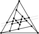
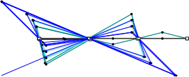
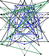
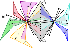
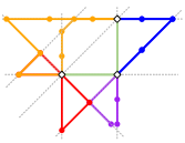
A segment in a straight-line drawing of a graph is a maximal set of edges that together form a line segment. The segment number of a planar graph is the minimum number of segments in any planar straight-line drawing of [9]. The line cover number of a planar graph is the minimum number of lines that support all the edges of a planar straight-line drawing of [6]. Clearly, for any graph [6]. As a side note, we show that for any connected graph . For circular-arc drawings of planar graphs, the arc number [27] and circle cover number [20] are defined analogously as the segment number and the line cover number, respectively, for straight-line drawings. For an example, see Fig. 1. All these numbers have been considered as meaningful measures of the visual complexity of a drawing of a graph; in particular, for the segment number, a user study has been conducted by Kindermann et al. [19].

In general, it is -complete [21] (and hence NP-hard) to compute the segment number of a planar graph. For the definition of the complexity class , see [26]. The segment number can, however, be computed efficiently for trees [9], series-parallel graphs of degree at most three [25], subdivisions of outerplanar paths [1], 3-connected cubic planar graphs [9, 15], and cacti [13]. Upper and lower bounds for the segment number of various graph classes are known, such as outerplanar graphs, 2-trees, planar 3-trees, 3-connected plane graphs [9], (4-connected) triangulations [10], and triconnected planar 4-regular graphs [13]. Some of the lower and upper bounds are so close that they yield constant-factor approximations, e.g., for outerplanar paths, maximal outerplanar graphs, 2-trees, and planar 3-trees [13]. Segment number and arc number have also been investigated under the restriction that vertices must be placed on a polynomial-size grid [27, 18, 14]. Also in the setting that a planar graph comes with a planar embedding (that is, for each face, the cyclic ordering of the edges around it is given and the outer face is fixed), it is NP-hard to compute the segment number of with respect to the given embedding [11].
This paper focuses on the parametrized complexity of computing the segment number of a graph. A decision problem with input and parameter is fixed-parameter tractable (FPT) if it can be solved by an algorithm with run time in where is a computable function, is the size of the input and is a constant. Given a planar graph and a parameter , the Segment Number problem is to decide whether . This is the natural parameter for the problem. By considering additional parameters, we get a more fine-grained picture of the complexity of the problem.
Chaplick et al. [7] showed that computing the line cover number of a planar graph is in FPT with respect to its natural parameter. They observed that, for a given graph and an integer , the statement can be expressed by a first-order formula about the reals. This observation shows that the problem of deciding whether or not lies in : it reduces in polynomial time to the decision problem for the existential theory of the reals. The algorithm of Chaplick et al. crucially uses the exponential-time decision procedure for the existential theory of the reals by Renegar [22, 23, 24] (see Section 2). Unfortunately, this procedure does not yield a geometric realization. Chaplick et al. even showed that constructing a drawing of a given planar graph that is optimal with respect to the line cover number can be unfeasible since there is a planar graph [7, Fig. 3b] such that every optimal drawing of requires irrational coordinates. They argue that any optimal drawing of contains the Perles configuration. It is known that every realization of the Perles configuration contains a point with an irrational coordinate [3, page 23]. Moreover, any optimal drawing of admits a cover with ten lines, and each of these lines contains a single line segment of the drawing. In other words, every drawing of that is optimal with respect to the line cover number is also optimal with respect to the segment number.
Our results.
We show that computing the segment number of a graph is FPT with respect to each of the following parameters: the natural parameter, the line cover number (both in Section 5), and the vertex cover number (in Section 4). Recall that the vertex cover number is the minimum number of vertices that have to be removed such that the remaining graph is an independent set. In the parametrized complexity community, the vertex cover number is considered a rather weak graph parameter, but for (geometric) graph drawing problems, FPT results can be challenging to obtain even with respect to the vertex cover number [4, 5, 2].
We remark that our algorithms use Renegar’s decision procedure as a subroutine; hence, when we compute the segment number of a planar graph , we do not get a straight-line drawing of that consists of line segments. Recall, however, that even specifying such a drawing is difficult for some graphs such as the above-mentioned graph , which has a point with irrational coordinates in any drawing that is optimal with respect to the segment number.
Motivated by list coloring, we also consider colored versions of the segment and line cover number problems. As a warm up, we provide efficient algorithms for computing the segment number of banana trees and banana cycles, that is, graphs that can be obtained from a tree or a cycle, respectively, by replacing each edge by a set of paths of length two; see Section 3.
Proofs for statements marked with can be found in the appendix.
2 Preliminaries
In a straight-line drawing of a graph, two incident edges are aligned if they are on the same segment. Since the number of segments equals the number of edges minus the number of pairs of aligned edges, we get the following.
Lemma 1
A planar straight-line drawing has the minimum number of segments if and only if it has the maximum number of aligned edges.
An existential first-order formula about the reals is a formula of the form , where consists of Boolean combinations of order and equality relations between polynomials with rational coefficients over the variables . Renegar’s result on the existential theory of the reals can be summarized as follows.
Theorem 2.1 (Renegar [22, 23, 24])
Given any existential sentence about the reals, one can decide whether is true or false in time
where is the number of variables in , is the number of polynomials in , is the maximum total degree over the polynomials in , and is the maximum length of the binary representation over the coefficients of the polynomials in .
The proof of the next lemma follows the approach in [7, Lemma 2.2].
Lemma 2 (lem:firstOrder*)
] Given an -vertex planar graph and an integer , there exists a first-order formula about the reals that involves polynomials in variables (each of constant total degree and with integer coefficients of constant absolute value) such that is satisfiable if and only if .
Corollary 1
Given an -vertex planar graph and an integer , there exists a -time algorithm to decide whether .
3 The Segment Number of Banana Trees and Cycles
We first consider some introductory examples. A banana is the union of paths that share only their start- and endpoints [28]. In this paper, we additionally insist that all paths have length 2. We say that a banana is a -banana if it consists of paths (of length 2). We call the joint endpoints of the paths covering vertices and the vertices in the interior of the paths independent vertices. Banana graphs, i.e., graphs in which some edges are replaced by bananas will play an important role in Section 4 when we consider the parameter vertex cover.
Lemma 3 ([9])
A -banana has segment number .
Proof
A -banana has edges. There is a drawing in which pairs of edges are aligned. See Fig. 2(a). This is optimum: At most one path of length two can be aligned at the independent vertex. If a pair of edges is aligned at one covering vertex then no pair can be aligned at the other covering vertex.

Given an integer , a banana path of length is a graph that is constructed from a path of length by replacing, for , edge of the path by a -banana, called banana , for some value . We say that is the multiplicity of edge ; see Fig. 2(b). Banana trees and banana cycles are defined analogously; see Fig. 3.
Theorem 3.1
The segment number of a banana path of length can be computed in time and can be expressed explicitly as a function of the multiplicities.
Proof
Let be a banana path of length with multiplicities . In each banana, align two edges at an independent vertex. At each inner covering vertex with , align edges from bananas and . In particular, we align the edges from incident bananas that were aligned at their respective independent vertex. Further, let . For each , let . Align pairs of edges of banana at covering vertex or , based on where the maximum is assumed. See Fig. 2(b). Note that setting takes into account that one edge is already aligned at an independent vertex. Therefore, it cannot be aligned at a covering vertex at the same time. It is not possible to align more pairs of edges. Thus, the segment number is .

The proof of the following theorem is in Appendix 0.B, Lemmas 6 and 7.
Theorem 3.2
The segment number of (i) a banana tree (ii) a banana cycle of length at least five where each banana contains at least two independent vertices can be computed in time linear in the number of covering vertices.
4 Parameter: Vertex Cover Number
In this section, we consider the following parametrized problem.
Let be a simple planar graph, and let be a vertex cover of with vertices. In order to compute the segment number of , we first compute a subgraph of whose size is in . We vary over all possible alignments of this subgraph and check whether they are geometrically realizable. We finally use an integer linear program (ILP) in order to reinsert the missing parts from . In the end, we take the best among the thus computed solutions. The details are as follows.
Dividing into equivalence classes.
Two vertices of are equivalent if and only if they are adjacent to the same set of vertices in . We say that an equivalence class is a -class if each vertex is adjacent to exactly vertices in . Observe that the -classes contain at most two vertices if . Otherwise would contain a , contradicting that is planar. Thus, the number of vertices in -classes, is bounded by .
Reducing the size of the graph.
Let be the graph obtained from by removing all vertices contained in 1-classes. Consider a planar embedding of . Let be a 2-class and let be adjacent to all vertices in . Observe that the edges between and do not have to be consecutive in the cyclic order around (and similarly for ). A contiguous 2-class is a maximal subset of such that the incident edges are consecutive around both and . Observe that two contiguous 2-classes are separated by the edge or by at least a vertex-cover vertex. Thus, a 2-class consists of at most contiguous 2-classes. Now, for each 2-class , we remove all but vertices from . Let the resulting graph be . Observe that the vertices of are the vertex cover vertices, the vertices of all -classes, , and at most vertices from each 2-class. Thus, the number of vertices of is bounded by .
Alignment within 2-classes.
For each 2-class , let be the edge connecting the two vertex cover vertices adjacent to the vertices in . We vary over all subsets of 2-classes for which is not an edge of . There are at most such subsets. For each , we add to . These edges represent a pair of aligned edges at an independent vertex. Let the resulting graph be .
Varying over all planar embeddings of .
For each 2-class , we replace each contiguous 2-class in by four vertices. The resulting four 2-paths represent the boundaries of two consecutive contiguous 2-classes; each of which shall be drawn in a non-convex way, i.e., such that the segment between the two incident vertex cover vertices does not lie in its interior. We call these non-convex quadrilaterals boomerangs. Let the thus constructed plane graph be .
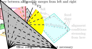
The reason why we represent each contiguous 2-class by two non-convex quadrilaterals instead of one arbitrary quadrilateral will become clear when we reinsert the 2-classes into the boomerangs; see also Fig. 4(b): Let , let and be the two vertex cover vertices incident to and assume that we have opted to draw into boomerang . Then we need to ensure that the edges and meet inside when we draw starting at and starting at independently of each other and with arbitrary slopes.

Alignment Requirements.
We vary over all possible “pairings” between edges and/or boomerangs incident to a common vertex that respect the embedding . If we require that two edges are aligned, that an edge should be aligned with an edge inside a boomerang, or that two edges inside different boomerangs can be aligned, we say that the respective edges and boomerangs are paired. E.g., Fig. 4(a) illustrates the following pairing around a vertex : the yellow boomerang is paired with the blue and the red boomerang as well as with the edge . The red and the green boomerangs are also paired. Edges and are paired. Edge is not paired with any other edge.
In order to handle pairings within boomerangs, we insert further edges into . See the dashed edges in Fig. 4(a). Let be a vertex cover vertex. Let be the neighbors of in this order around . Assume that and are two independent vertices representing the border of a boomerang . Assume that we would like to align the edges around such that should get aligned with some edges in if any. Then we add up to edges incident to inside the region representing and require them to be aligned with the respective edges among at .
E.g., when we consider the yellow boomerang in Fig. 4(a) then , . Since we require the red boomerang to be partially paired with (we also want it to be paired with the green one), we only add a counterpart for one of the boundary edges, , inside . The blue boomerang should be exclusively paired with , so we add counter parts for both boundary edges, and . Edge should be aligned with an edge in , so it also gets a counterpart in . According to the currently chosen pairing , the edge does not have to be aligned in , so we do not add a counterpart for it in .
We do this operation for each boomerang and each incident vertex cover vertex. The resulting graph has at most thrice as many edges as .
Testing and optimally reinserting the 1- and 2-class vertices.
We now have a plane graph with vertices. See Fig. 5. Some pairs of edges are required to be aligned. The two 2-paths representing the boundary of a boomerang must bound a quadrilaterial that does not contain the segment between the two vertex cover vertices. We use Renegar’s algorithm [22, 23] to test whether these requirements are geometrically realizable.
Lemma 4 (lem:realize-G-two*)
] Given a plane graph with embedding and vertices, a set of pairs of edges, a set of 4-cycles of , and for each 4-cycle in a specified diagonal , we can decide, in time, whether there exists a planar straight-line drawing of such that (i) the edge pairs in are aligned and (ii) for each 4-cycle in , does not lie in the interior of or on .
We apply Lemma 4 to , setting according to , to the set of all boomerangs, and, for each boomerang , the specified diagonal to the segment between the two vertex cover vertices. If the answer is yes, we set up and solve the following ILP to optimally insert 2-class vertices into the boomerangs and to optimally add the 1-class vertices. To this end, we use, among others, the following variables: expresses how many edges in boomerang should be aligned to edges in boomerang at vertex and expresses how many edges between and 1-class vertices should be aligned with edges in boomerang . We allow that some of the boomerangs remain empty. The ILP uses variables and constraints and, thus, can be solved in time [17, 16, 12]. For details, see Appendix 0.C.
We are now ready to prove the main theorem of this section.
Theorem 4.1
Segment Number by Vertex Cover Number is FPT.
Proof
The vertex cover number of the input graph with vertices can be computed in time [8]. The number of subsets of 2-classes is in . Then we vary over all embeddings of ; see the respective paragraph on Section 4. The number of embeddings of the graph with vertices is in for some constant , and the number of possible pairings is also bounded by a function of . The plane graph has vertices. Hence, testing whether the alignment and non-convexity requirements of can be realized geometrically can be done in time. If the answer is yes, we can solve the ILP in time. In the end we have to determine the minimum over all choices of , , .
In order to prove correctness, consider now a hypothetical geometric realization and an optimum solution of the ILP. Observe that the ILP is always feasible. It remains to show that the 2-class vertices can be inserted into the boomerangs and the 1-class vertices can be added so as to fulfill the alignment requirements prescribed by the ILP. For each triplet , where and are two boomerangs incident to a common vertex cover vertex , we add stubs of aligned edges in a close vicinity of inside the region reserved for and . Further, for each boomerang incident to a vertex cover vertex do the following. For each edge of that we required to be aligned with an edge in at , we add a stub incident to into aligned with . We also add stups incident to into . If the total number of stubs in all boomerangs representing contiguous subclasses of a 2-class are less than , we add more stubs into arbitrary boomerangs associated with . We extend the stubs until the respective rays meet. Observe that this intersection point is inside the boomerang and that no crossings are generated; see Fig. 4(b).
5 Parameters: Segment and Line Cover Number
In this section, we first study the parameterized complexity of computing the segment number of a planar graph with respect to the segment number and the line cover number separately. Recall that, if , then . Then, we study the parameterized complexity of colored versions of the segment number and the line cover number with respect to their natural parameters.
We start by reviewing an FPT algorithm for the line cover number [7]. A path component (resp., cycle component) of a graph is a connected component isomorphic to a path (resp., a cycle). The algorithm first removes all the path components of the input graph , as they can be placed on a common line. Then each of the remaining connected components of is reduced by replacing long maximal paths. More precisely, paths of length greater than that contain only vertices of degree at most are replaced by paths of length . Indeed, vertices of degree 2 are irrelevant since they can always be reintroduced by subdividing a straight-line segment of the path in a feasible solution of the reduced instance to obtain a feasible solution of the original instance. Note that the number of vertices of degree greater than must be at most . This yields an equivalent instance with at most vertices and edges. Next, the algorithm implicitly enumerates all line arrangements of lines. For each such arrangement, the algorithm enumerates all possible placements of the vertices of at crossing points in the arrangement. Observe that the vertices of degree greater than must be placed at the crossing points of the lines. The instance is accepted if at least one of the line arrangements can host .
In order to explicitly enumerate all line arrangements of lines (as needed in Algorithm 1), we can proceed as described below. Observe that a line arrangement of lines defines a connected straight-line plane graph as follows. The graph contains, for each crossing point in , a vertex , and, for every pair of crossing points and that appear consecutively along a line of , an edge . Additionally, for each half-line of that starts at a crossing point , the graph contains a leaf adjacent to . The clockwise order of the edges around each vertex of (of degree larger than ) is naturally inherited from the order of the crossing points of around . By construction, defines a unique connected straight-line plane graph together with a unique covering of the edges of with edge-disjoint paths starting and ending at leaves. Thus, to enumerate all line arrangements of lines, we execute the following steps. We consider all possible planar graphs on vertices containing leaves, all their planar embeddings, and all their edge coverings with edge-disjoint paths, if any. For each such triplet (of a planar graph, an embedding, and an edge covering), we test (using again Renegar’s algorithm [22, 23]) whether the considered graph admits a straight-line planar drawing preserving the selected embedding, in which each edge-disjoint path of the considered covering is drawn on a straight-line. Each triplet that passes the previous test corresponds to a (combinatorially different) line arrangement of lines.
To compute the segment number of , first observe that each path component requires a segment in a drawing of . Assume that has path components. Then, let be our new parameter and remove the path components from . Also, observe that the choices above only leave undecided to which line of the arrangement the hanging paths of , i.e., the paths that start at a high degree vertex and end at a degree- vertex, are assigned. Clearly, the number of such choices are also bounded by a function of . Therefore, for every line arrangement and every placement of the vertices of to the crossing points of the arrangement, we consider all possible ways to assign the hanging paths to the lines and compute the actual number of segments determined by these choices. We conclude that if and only if we encountered a line arrangement and a placement of vertices of in this line arrangement that determines at most segments. This immediately implies the following theorem.
Theorem 5.1
Segment Number is FPT with respect to the natural parameter.
Note that the line cover number is lower or equal to the segment number. However, assuming no path component exists, we can show that the segment number is polynomially bounded by the line cover number (see Proposition 1 in Appendix 0.D). This and Theorem 5.1 yield the following theorem.
Theorem 5.2 (the:segByLineCover*)
] Computing the segment number is FPT parameterized by the line cover number of the input graph.
Motivated by list coloring, we generalize both Segment Number and Line Cover Number by prescribing admissible segments or lines for certain edges.
Theorem 5.3
The problems List-Incidence Line Cover Number and List-Incidence Segment Number are FPT with respect to the natural parameter.
Note that Theorem 5.3 generalizes Theorem 5.1, but the algorithm for Segment Number, which yields Theorem 5.1, is faster than the algorithm for List-Incidence Segment Number. Our main tool to prove Theorem 5.3 is the next lemma, which proves the theorem assuming that the input does not contain any path or cycle components. In Appendix 0.F, we show how to solve the remaining technicalities.

Lemma 5
The problems List-Incidence Line Cover Number and List-Incidence Segment Number are FPT with respect to the natural parameter for instances containing no path or cycle components.
Proof
We first consider the List-Incidence Line Cover Number problem. Note that a feasible instance can have at most vertices of degree greater than . Let be the subgraph of induced by vertices of degree greater than . We enumerate all possible arrangements of lines and all possible placements of vertices of of degrees greater than in the crossing points of the lines. The placement of vertices determines a straight-line drawing of , (see green edges in Fig. 6). We continue with the considered arrangement/vertex-placement pair only if the drawing of is proper, i.e., it is planar, and each edge of belongs to a line of the arrangement and does not pass through another vertex of degree greater than . Sections of lines between consecutive crossing points not occupied by edges of are called intervals. Let and be two intervals. is aligned to (in this order) if they belong to the same line and the ending point of is the starting point of . is adjacent to (in this order) if they do not belong to the same line and the ending point of is the starting point of .
Now consider a path in such that , i.e., , , and is either or greater than . We call such a path light. Consider the representation of a light path in a solution. The path leaves the vertex along some line, then turns to another line, possibly several times, until it either ends in a crossing point, where vertex had been placed (when ) or in an inner point of some interval (when , note that w.l.o.g. we may assume that vertices of degree are not placed in crossing points). This describes the routing of . Every maximal sequence of consecutive intervals that belong to the same line will be called a superinterval in the routing. In particular, we can represent a routing of by the sequence of superintervals such that and are consecutive. Every two consecutive intervals within a superinterval are aligned, while for two consecutive superintervals, the last interval of the first one is adjacent to the first interval of the second one (see Fig. 6).
We use the following strategy. For every light path, we select its routing as a sequence of superintervals. Moreover, we enumerate over all possible namings of the lines of the arrangement with labels in and proceed only with those namings that determine a compatible drawing of , i.e., one in which, for each edge of , it holds that lies on a line in .
Let be a collection of routings for the light paths. We check if is feasible, i.e., any two routings in are non-crossing and internally disjoint, and each of them is internally disjoint with the drawing of . For every light path, we check if the lists assigned to each of its edge allow its allocation along this routing. The first superinterval of a routing must start in vertex . The last one must end in if . (If , there is no restriction on .)
The strategy described above is summarized in Algorithm 1. To check whether the lists assigned to the edges of a path allow their allocation along a given routing, Algorithm 1 exploits the procedure CheckRouting (see Algorithm 2), which works as follows.
For a light path and a routing , we fill in a table via dynamic programming. Its meaning is that true if and only if the subpath is realizable along , i.e., it admits a planar geometric realization such that all the vertices are placed inside the superintervals of and every edge lies on a line in the list .
The correctness of Algorithm 1 follows from the fact that we are performing an exhaustive exploration of the solution space. The correctness of Algorithm 2 follows from the fact that can be realized along the initial part of so that vertex is placed inside the superinterval if and only if can be realized so that is placed on the crossing point that is the last point of . The former is used (and needed) when updating to , the latter for updating to .
The following claim states that Algorithm 1 is FPT with respect to .
Claim 1 (cla:algoListLineNumber*)
] Let be the time needed to enumerate all non-isomorphic line arrangements of lines. Then Algorithm 1 runs in time .
We now consider the List-Incidence Segment Number problem. As already mentioned, any realization with segments is itself a realization with at most lines. Thus, we can use Algorithm 1, with just two slight modifications. Observe that, in the third for loop of the algorithm, the considered collection of routings of the light paths together with the drawing of uniquely determines the segments of the representation. Therefore, we only proceed to the fourth for loop with those collections that determine at most segments. However, if we proceed, in the fourth for loop, we consider all possible namings of these segments instead of considering all possible namings of the lines of the current arrangement. Clearly, the notion of compatible drawing of is naturally modified using the segment labels. Finally, note that counting the number of segments affects the running time by a factor that depends solely on .
6 Open Problems
We have shown that segment number parameterized by segment number, line cover number, and vertex cover number is fixed parameter tractable. Another interesting parameter would be the treewidth. So far, even for treewidth 2, efficient optimal algorithms are only known for some subclasses [1, 25, 13].
The cluster deletion number of a graph is the minimum number of vertices that have to be removed such that the remainder is a union of disjoint cliques. Clearly, the cluster deletion number is always upper-bounded by the vertex cover number. Is the segment number problem FPT w.r.t. the cluster deletion number?
References
- [1] Adnan, M.A.: Minimum Segment Drawings of Outerplanar Graphs. Master’s thesis, Department of Computer Science and Engineering, Bangladesh University of Engineering and Technology (BUET), Dhaka (2008), http://lib.buet.ac.bd:8080/xmlui/bitstream/handle/123456789/1565/Full%20%20Thesis%20.pdf?sequence=1&isAllowed=y
- [2] Balko, M., Chaplick, S., Gupta, S., Hoffmann, M., Valtr, P., Wolff, A.: Bounding and computing obstacle numbers of graphs. In: Chechik, S., Navarro, G., Rotenberg, E., Herman, G. (eds.) Proc. 30th Europ. Symp. Algorithms (ESA’22). LIPIcs, vol. 244, pp. 11:1–13. Schloss Dagstuhl – Leibniz-Zentrum für Informatik (2022). https://doi.org/10.4230/LIPIcs.ESA.2022.11
- [3] Berger, M.: Geometry Revealed: A Jacob’s Ladder to Modern Higher Geometry. Springer (2010). https://doi.org/10.1007/978-3-540-70997-8_1
- [4] Bhore, S., Ganian, R., Montecchiani, F., Nöllenburg, M.: Parameterized algorithms for book embedding problems. JGAA 24(4), 603–620 (2020). https://doi.org/10.7155/jgaa.00526
- [5] Bhore, S., Ganian, R., Montecchiani, F., Nöllenburg, M.: Parameterized algorithms for queue layouts. JGAA 26(3), 335–352 (2022). https://doi.org/10.7155/jgaa.00597
- [6] Chaplick, S., Fleszar, K., Lipp, F., Ravsky, A., Verbitsky, O., Wolff, A.: Drawing graphs on few lines and few planes. J. Comput. Geom. 11(1), 433–475 (2020). https://doi.org/10.20382/jocg.v11i1a17
- [7] Chaplick, S., Fleszar, K., Lipp, F., Ravsky, A., Verbitsky, O., Wolff, A.: The complexity of drawing graphs on few lines and few planes. JGAA 27(6), 459–488 (2023). https://doi.org/10.7155/jgaa.00630
- [8] Chen, J., Kanj, I.A., Xia, G.: Improved upper bounds for vertex cover. Theor. Comput. Sci. 411(40-42), 3736–3756 (2010). https://doi.org/10.1016/j.tcs.2010.06.026
- [9] Dujmović, V., Eppstein, D., Suderman, M., Wood, D.R.: Drawings of planar graphs with few slopes and segments. Comput. Geom. 38, 194–212 (2007). https://doi.org/10.1016/j.comgeo.2006.09.002
- [10] Durocher, S., Mondal, D.: Drawing plane triangulations with few segments. Comput. Geom. 77, 27–39 (2019). https://doi.org/10.1016/j.comgeo.2018.02.003
- [11] Durocher, S., Mondal, D., Nishat, R., Whitesides, S.: A note on minimum-segment drawings of planar graphs. JGAA 17(3), 301–328 (2013). https://doi.org/10.7155/jgaa.00295
- [12] Frank, A., Tardos, É.: An application of simultaneous diophantine approximation in combinatorial optimization. Combinatorica 7(1), 49–65 (1987). https://doi.org/10.1007/BF02579200, https://doi.org/10.1007/BF02579200
- [13] Goeßmann, I., Klawitter, J., Klemz, B., Klesen, F., Kobourov, S.G., Kryven, M., Wolff, A., Zink, J.: The segment number: Algorithms and universal lower bounds for some classes of planar graphs. In: Bekos, M.A., Kaufmann, M. (eds.) WG 2022. LNCS, vol. 13453, pp. 271–286. Springer (2022). https://doi.org/10.1007/978-3-031-15914-5_20
- [14] Hültenschmidt, G., Kindermann, P., Meulemans, W., Schulz, A.: Drawing planar graphs with few geometric primitives. JGAA 22(2), 357–387 (2018). https://doi.org/10.7155/jgaa.00473
- [15] Igamberdiev, A., Meulemans, W., Schulz, A.: Drawing planar cubic 3-connected graphs with few segments: Algorithms & experiments. JGAA 21(4), 561–588 (2017). https://doi.org/10.7155/jgaa.00430
- [16] Jr., H.W.L.: Integer programming with a fixed number of variables. Math. Oper. Res. 8(4), 538–548 (1983). https://doi.org/10.1287/moor.8.4.538, https://doi.org/10.1287/moor.8.4.538
- [17] Kannan, R.: Minkowski’s convex body theorem and integer programming. Math. Oper. Res. 12(3), 415–440 (1987). https://doi.org/10.1287/moor.12.3.415, https://doi.org/10.1287/moor.12.3.415
- [18] Kindermann, P., Mchedlidze, T., Schneck, T., Symvonis, A.: Drawing planar graphs with few segments on a polynomial grid. In: Archambault, D., Tóth, C.D. (eds.) GD 2019. LNCS, vol. 11904, pp. 416–429. Springer (2019). https://doi.org/10.1007/978-3-030-35802-0_32
- [19] Kindermann, P., Meulemans, W., Schulz, A.: Experimental analysis of the accessibility of drawings with few segments. JGAA 22(3), 501–518 (2018). https://doi.org/10.7155/jgaa.00474
- [20] Kryven, M., Ravsky, A., Wolff, A.: Drawing graphs on few circles and few spheres. JGAA 23(2), 371–391 (2019). https://doi.org/10.7155/jgaa.00495
- [21] Okamoto, Y., Ravsky, A., Wolff, A.: Variants of the segment number of a graph. In: Archambault, D., Tóth, C.D. (eds.) GD 2019. LNCS, vol. 11904, pp. 430–443. Springer (2019). https://doi.org/10.1007/978-3-030-35802-0_33
- [22] Renegar, J.: On the computational complexity and geometry of the first-order theory of the reals. Part I: Introduction. Preliminaries. The geometry of semi-algebraic sets. The decision problem for the existential theory of the reals. J. Symb. Comput. 13(3), 255–299 (1992). https://doi.org/10.1016/S0747-7171(10)80003-3
- [23] Renegar, J.: On the computational complexity and geometry of the first-order theory of the reals. Part II: The general decision problem. Preliminaries for quantifier elimination. J. Symb. Comput. 13(3), 301–327 (1992). https://doi.org/10.1016/S0747-7171(10)80004-5
- [24] Renegar, J.: On the computational complexity and geometry of the first-order theory of the reals. Part III: Quantifier elimination. J. Symb. Comput. 13(3), 329–352 (1992). https://doi.org/10.1016/S0747-7171(10)80005-7
- [25] Samee, M.A.H., Alam, M.J., Adnan, M.A., Rahman, M.S.: Minimum segment drawings of series-parallel graphs with the maximum degree three. In: Tollis, I.G., Patrignani, M. (eds.) GD 2008. LNCS, vol. 5417, pp. 408–419. Springer (2008). https://doi.org/10.1007/978-3-642-00219-9_40
- [26] Schaefer, M.: Complexity of some geometric and topological problems. In: Eppstein, D., Gansner, E.R. (eds.) GD 2009. LNCS, vol. 5849, pp. 334–344. Springer-Verlag (2010). https://doi.org/10.1007/978-3-642-11805-0_32
- [27] Schulz, A.: Drawing graphs with few arcs. JGAA 19(1), 393–412 (2015). https://doi.org/10.7155/jgaa.00366
- [28] Scott, A., Seymour, P.: Induced subgraphs of graphs with large chromatic number. VI. Banana trees. J. Combin. Theory Ser. B 145, 487–510 (2020). https://doi.org/10.1016/j.jctb.2020.01.004
Appendix
Appendix 0.A Proofs Omitted in Section 2
See 2
Proof
Note that we can return true immediately if . Otherwise, the formula needs to model the fact that there are pairs of points, determining a set of lines, and that there are distinct points representing the vertices of such that the segments corresponding to the edges of lie on the lines in and do not overlap or cross each other or leave gaps on the lines. For details on how to encode this, see [7, Lemma 2.2].
Appendix 0.B Proofs Omitted in Section 3
Lemma 6
The segment number of a banana tree can be computed in time linear in the number of covering vertices.
Proof
Let be a banana tree constructed from a tree . For an edge of , let be the multiplicity of and let be the set of edges incident to that are contained in the -banana inserted for . For each banana, align the two edges incident to one independent vertex. For each leaf of , align the remaining edges of the respective banana – up to at most two – at . Let be an inner vertex of , and let be the neighbors of in . Align as many pairs of edges from different bananas at . These are all (except possibly one) edges if there is no such that . If there is a -banana that is large at , i.e., if for some then align some edges inside the respective -banana at – or at if the -banana is also large at and the alignment at this end would be more beneficial. More precisely: let be the neighbors of in . Then align pairs of edges within at or pairs of edges within at , depending on which number is larger. Observe that at any vertex this condition always holds for at most one banana, so there are no conflicts. Locally, this yields an optimal assignment.

The respective alignment can be realized geometrically: We root at a degree one vetex . All but at most two edges incident to must be aligned at and two edges incident to one independent vertex incident to must also be aligned. This can be realized as in Fig. 2(a). In general, we have now the following situation, we have drawn the bananas contained in a subtree of . All vertices of that are incident to vertices not yet in are leaves of . Let be such a leaf of and let be the ancestor of in . Let be the set of edges that should be aligned with edges in other bananas and let be the edges that are aligned with each other. We maintain the property that the maximum angle between two edges of is less than . Thus, if then encloses . Moreover, for each leaf of , we maintain disjoint circles around that contain or intersect at most edges from . We now insert the subtree rooted at into these circles maintaining the alignment requirements, the disjoint circles and the above mentioned drawing requirements. See Fig. 7 for different cases. Observe that if then there might be a different large banana at (the red banana in Fig. 7(b)). Since the maximum angle at between two edges in is less than it follows that we can always fit this large banana.
Observe that the strategy of locally optimal alignments would no longer work for simple cycles. E.g. assume each edge in a simple cycle was replaced by a 1-banana. Then locally, all pairs of incident edges should be aligned, both, at vertices of the simple cycle and at the independent vertices. But this is not realizable geometrically. Instead the segment number would be 3. Some examples of segment-minimum drawings of cycles of 4-bananas are shown in Fig. 3.
Lemma 7
The segment number of a banana cycle of length at least five can be computed in linear time in the number of covering vertices if each banana contains at least two independent vertices.
Proof
Let be a banana cycle of length at least five with the property that each banana contains at least two independent vertices. Let be a maximal subgraph of such that is a regular banana cycle, i.e., such that each banana contains the same number of independent vertices. In Fig. 3(b) this is the subgraph induced by the black, gray, blue, and lightblue edges. Depending on whether the length of the cycle is odd or even, draw as indicated in Fig. 3 for banana cycles of length 5 or 6 starting with the one or two cycles, respectively, containing pairs of edges aligned at independent vertices (black and gray). Removing the edges of from yields a union of banana paths. We align edges according to the rules for banana paths without aligning edges at independent vertices (edges in different shades of green).
Appendix 0.C Proofs Omitted in Section 4
See 4
Proof
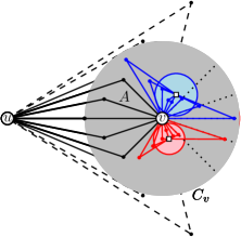
We use the following simple tool from geometry. Given three points , , in the plane, let
be the scalar triple product of three 3-dimensional vectors , , and . As is well known, the following conditions are equivalent:
-
•
;
-
•
, and the point lies in the left halfplane with respect to the oriented line through and , oriented from to ;
-
•
the points , , and are pairwise distinct, non-collinear, and occur counterclockwise in the circumcircle of the triangle in this order.
Moreover, if and only if the points , , and are collinear, including the case that some of them coincide.
Let be the vertex set of . We want to express the fact that there are pairwise distinct points that determine a straight-line drawing of . Our existential statement about the reals begins, therefore, with the quantifier prefix
For each pair of edges and such that follows immediately in the counterclockwise cyclic ordering of the edges incident to according to , we add to the constraint (using conjugation).
For each 4-cycle with , we add to the constraint . In other words, and must have the same (non-zero) sign.
If there is a pair of edges in that is not incident, we can reject the instance. For each pair of edges and in , we add to the constraint . (We could also express that must lie in the relative interior of the line segment , but this is implied automatically by the ordering of the edges around – if there is another edge incident to . If not, we can remove and replace the path by the straight-line edge .)
For each pair of non-incident edges and of , we need to ensure that and do not cross each other. This can be expressed using the relation defined in the proof of [7, Lemma 2.2].
Note that involves polynomials in variables, each of constant total degree and with integer coefficients of constant absolute value. Using Renegar’s result (Theorem 2.1), we can test whether admits a solution over the reals in time.
Description of the ILP.
We explain the ILP for the optimal distribution of 2-class and 1-class vertices by example. Let and be the two gray boomerangs in Fig. 5 with vertex cover vertices and , let be the boomerangs that are incident to and paired with , and let and be the boomerangs incident to and paired with . (Additionally, boomerang is paired with boomerang .)
With the respective upper case letters we will denote the respective 2-classes. E.g., is the 2-class whose vertices are adjacent to and since the boomerangs and represent contiguous subsets of . For a 2-class , let be the size of – minus one if , i.e., if one 2-path through a vertex of was already modeled by the edge . For the ILP, is a constant.
Let now and be two boomerangs that are paired at the vertex cover vertex . We introduce an integer variable for the number of pairs of edges such that is in , is in , and and are aligned at .
For each vertex , let be the number of leaves (1-classes) incident to . For the ILP, is a constant. Further, we introduce an integer variable for the number of leaves incident to that are aligned with edges assigned to a boomerang , and a variable for the number of pairs of leaves incident to that are aligned with each other. Then, is an upper bound to the sum of all leaves that are aligned with edges of any boomerang incident to plus twice the number of pairs of leaves that are aligned with each other. For vertices and in Fig. 5, this yields the constraints
For each vertex , let be defined as follows:
For example, in Fig. 5, we have
Then our objective is to
For a boomerang incident to vertex cover vertex , let be the number of edges of that are paired at with edges of . For the ILP, is a constant. For example, in Fig. 5, due to the edge in , whereas . We need only one more type of constraints. We establish, for each boomerang representing a contiguous subclass of the 2-class , a bound for the number of vertices that have to be contained in in order to satisfy the alignment requirements.
We also do this for all other 2-classes. Now the following constraint says that the total number of vertices that we distribute to the boomerangs associated with the 2-class is at most . In our example, we have
Note that the edges that belong to aligned pairs coming into a boomerang from one side can always be completed to paths of length 2, either with edges that belong to aligned pairs entering the boomerang from the other side or with usual unconstrained edges.
It remains to analyze the numbers of variables and constraints. Recall that the number of vertices and edges of the plane graph is in . The number of variables of type and is bounded by the number of edges and, thus, is also in . The number of variables of type and is obviously in . Finally, for a fixed vertex cover vertex , the number of variables of type is bounded by : If is only paired with , then we assign the cost for the variables to . If both, and are not only paired with each other, we assign the cost of to and the cost of to . Observe that this happens at most twice for each boomerang incident to . Thus, by the hand shaking lemma, the total number of variables of type is bounded by the number of edges, which is again in . There is one constraint for each 1-class, one constraint for each variable of type , two constraints for each variable of type , and one constraint for each 2-class. Thus, the total number of constraints is in .
Appendix 0.D Parameter: Line Cover Number
In this section, we show that computing the segment number is FPT parameterized by the line cover number.
We exploit the following observation.
Proposition 1
Let be the connected components of a graph . The following hold:
-
1.
.
-
2.
Let be the path components of and let . Then, . Moreover, if then , and otherwise.
-
3.
If contains no path component, then .
Proof
Items 1 and 2 are obvious. For the last item, consider a drawing of on lines. Since has no path component, every segment of must contain at least one of the at most crossing points of the line that supports it. Different segments supported by the same line are disjoint. Therefore, the number of segments of cannot exceed .
See 5.2
Proof
Suppose that we are given an input graph with . We first identify its connected components. Let be the number of path components of . Delete the path components of , if any, to obtain a graph for which . So the segment number of is bounded by a function of and hence, by Theorem 5.1, can be computed in FPT time parameterized by . Once is computed, output , by Item 3 of Proposition 1.
Appendix 0.E Proofs Omitted in Section 5
See 1
Proof
Recall that, there are nested for loops in Algorithm 1. For the running time estimate of Algorithm 1, we note first that Algorithm 2 takes time since the table has entries and the update step requires searching through an at-most--element list. Since and the number of superintervals on a routing cannot exceed the total number of intervals, which is no more than , the running time of Algorithm 2 is upper bounded by . Since both the light paths and the routings in a collection of paths/routings are pairwise disjoint, is actually an upper bound on the total execution time of the innermost (fifth) for loop of Algorithm 1, where the procedure CheckRouting is called on every light path and a corresponding given routing for the path.
Clearly, the number of non-isomorphic line arrangements of lines is upper bounded by the number of graphs on vertices, i.e., . Therefore, the enumeration of all such arrangements in the outermost (first) for loop can be performed in time, where is a computable function [7].
Since there are at most crossing points of the lines, the vertices of degree greater than can be placed in at most ways, which bounds the number of times the second for loop is executed.
Inside the second for loop, we first check if is proper. For this, we test for each edge of , if it belongs to a line of the arrangement and if it does not pass through any vertex of . There are edges to be checked and on each of them at most other crossing points that could create a conflict, and so this check can be performed in time. (This also includes checking if no two edges of cross.)
In a feasible instance, there is no more than light paths, because they start in one of at most vertices and in each starting vertex, the first edge of the path has at most choices (there are at most lines passing through this point, and on each of them two possible directions to be used). A routing of a light path is a sequence of at most superintervals since each line may host at most disjoint superintervals. The first superinterval on a routing can be chosen in at most ways (the routing chooses a line to follow, the direction, and the last point of this superinterval). Similarly, the second superinterval can be chosen in ways, etc. Thus routing one path can be chosen in at most ways, and the collection of routing in ways. Thus the number of choices in the third for loop is at most .
Since there exists at most ways of the naming of the lines of the arrangement, the fourth for loop introduces a multiplicative factor of in the running time.
Therefore, the overall running time of Algorithm 1 is
Thus the algorithm is FPT when parameterized by .
Appendix 0.F Handling Path and Cycle Components in the proof of Theorem 5.3
Now, we show how to handle cycle and path components. Somewhat surprisingly, paths are the most troublemaking components.
First, we consider the cycle components. A cycle component cannot be drawn on a line, and thus any of its drawings must bend in a crossing point. Then it can be described by a closed routing of superintervals, and we include such a routing in the third for loop of Algorithm 1. The subroutine CheckRouting is modified as follows: We pick one of the bending points and try all possibilities which vertex of the component is placed in this crossing point and in which direction the cycle travels around the chosen cyclic routing. This adds a multiplicative factor to the overall running time of the algorithm.
Second, we consider the path components. Consider a path component . If has a universal index, i.e., if there is an index which belongs to all , we can realize this path on line in some sector which does not belong to any routing nor to edges of (in case of List-Incidence Line Cover Number) not affecting the realizability of rest of the graph. Thus, such paths can be ignored for List-Incidence Line Cover Number.
However, in the List-Incidence Segment Number problem, it may be favourable to use bends even if the path has a universal index in the lists of its vertices, as this may prevent other components of the graph to be routed along the segment corresponding to the universal index. Moreover, even if we decide to route the path along a segment corresponding to one of the universal indices of the path, the feasibility of the instance may depend on which index we use. However, since the segment number of a graph equals the sum of the segment numbers of its connected components, the number of components of a feasible instance is always bounded by . Thus, for every path component , we check whether the set of universal indices, i.e, , is non-empty. If this is the case, we (i) decide whether we realize as a single segment, and if so, (ii) what is the index of this segment. This leaves possibilities to try, and for each of them, we delete the index of this segment from all lists of other components. Then we proceed with the rest of graph. Altogether, we have refined the search tree by a factor of .
For paths with a universal index that were chosen to be represented with bends, and for paths that must be realized with bends (since they do not have any universal index), we use the routing approach (both in case of List-Incidence Segment Number and List-Incidence Line Cover Number) as described in the case of cycle components. Therefore, processing these components affects the running time by a multiplicative factor of .