On the variance of the Fibonacci partition function

Abstract.

We determine the order of magnitude of the variance of the Fibonacci partition function. The answer is different to the most naive guess. The proof involves a diophantine system and an inhomogeneous linear recurrence.

1. Introduction

The Fibonacci partition function $R(n)$ counts solutions to

$$x_{1}+\cdots+x_{s}=n,$$

where $x_{1}<\cdots<x_{s}$ are Fibonacci numbers. Its values form the sequence OEIS A000119. By Zeckendorf’s theorem, which uniquely expresses a positive integer as a sum of non-consecutive Fibonacci numbers, we have

$$R(n)\geqslant 1\qquad(n\in\mathbb{N}).$$

Observe that $R(0)=1$, since the empty sum vanishes, and that

$$R(n)=0\qquad(n<0).$$

Several recursive formulas have been provided over the years [1, 4, 6]. Most recently, Chow and Slattery [2] furnished a fast, practical algorithm to compute $R(n)$, based on the Zeckendorf expansion.

The summatory function

$$A(H)=\sum_{n=0}^{H}R(n)$$

was shown in [2] to have order of magnitude $H^{\lambda}$, where

$$\varphi=\frac{1+\sqrt{5}}{2},\qquad{\lambda}=\frac{\log 2}{\log\varphi}\approx 1.44.$$

Thus, the average $(H+1)^{-1}\sum_{n=0}^{H}R(n)$ behaves fairly nicely, having order of magnitude $H^{{\lambda}-1}$. Chow and Slattery [2] demonstrated that $\displaystyle\lim_{H\to\infty}H^{-{\lambda}}A(H)$ does not exist. There it was also found that $\displaystyle\lim_{m\to\infty}F_{m}^{-{\lambda}}A(F_{m})$ does exist, and such limits were recently investigated in far more generality by Zhou [7].

The Fibonacci partition function is highly erratic. A simple exercise reveals, perhaps surprisingly at first, that

$$R(F_{m}-1)=1\qquad(m\geqslant 2).$$

At the other extreme, Stockmeyer [5] showed that

$$R(F_{m}^{2}-1)=F_{m}\qquad(m\geqslant 2),$$

and moreover

$$R(n)\leqslant\sqrt{n+1}$$

with equality if and only if we have $n=F_{m}^{2}-1$ for some $m\geqslant 2$.

In this article, we quantify the fluctuations of $R(n)$ by estimating the second moment

$$V(H):=\sum_{n=0}^{H}R(n)^{2}.$$

By Cauchy–Schwarz, we have

$$V(H)\geqslant H^{-1}A(H)^{2}\gg H^{2{\lambda}-1}.$$

If the function $R(n)$ were not too erratic, then we would have $V(H)\asymp H^{2{\lambda}-1}$. One might naively guess this if computers were less powerful, see Figure 1.1.

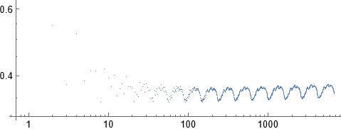
Figure 1.1. $V(H)H^{1-2\lambda}$ against $H$ for $1\leqslant H\leqslant 6765$

However, the growth of $V(H)H^{1-2\lambda}$ becomes clearer with more data, see Figure 1.2.

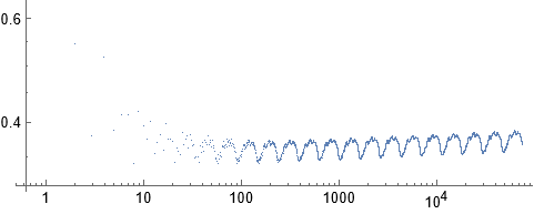
Figure 1.2. $V(H)H^{1-2\lambda}$ against $H$ for $1\leqslant H\leqslant 75025$

We find that $V(H)$ grows like a slightly larger power of $H$.

Theorem 1.1.

Let ${\lambda}_{1}\approx 2.48$ be the greatest root of the polynomial

$$x^{3}-2x^{2}-2x+2.$$

Then, for $H\in\mathbb{N}$, we have

$$V(H)\asymp H^{(\log{\lambda}_{1})/\log\varphi}.$$

The exponent

$$\frac{\log{\lambda}_{1}}{\log\varphi}\approx 1.89$$

slightly exceeds the Cauchy–Schwarz exponent

$$2{\lambda}-1\approx 1.88.$$

Notation

We employ the usual Bachman–Landau and Vinogradov asymptotic notations. For positive-valued functions $f$ and $g$, we write:

• $f\ll g$, if $|f|\leqslant C|g|$ pointwise, for some constant $C$,

• $f\asymp g$, if $f\ll g\ll f$,

• $f\sim g$, if $f/g\to 1$ in some specified limit.

Organisation and methods

In §2, we interpret $V(F_{m})-V(F_{m-1})$ as the number of solutions to a system comprising a diophantine equation and two inequalities. A case analysis then leads to a recurrence for $V(F_{m})$. We then solve the inhomogeneous linear recurrence in §3, delivering an exact formula and hence an asymptotic formula for $V(F_{m})$. From there, we deduce Theorem 1.1.

Funding

OJ was supported by a URSS bursary from the University of Warwick.

Rights

For the purpose of open access, the authors have applied a Creative Commons Attribution (CC-BY) licence to any Author Accepted Manuscript version arising from this submission.

2. A diophantine system

We start by analysing the variance along the Fibonacci sequence.

Lemma 2.1.

For $m\geqslant 7$, we have

$$V(F_{m}) =2V(F_{m-1})+3V(F_{m-2})-4V(F_{m-3})-2V(F_{m-4})+2V(F_{m-5})$$

$$\qquad+1-2\lfloor m/2\rfloor.$$

We will repeatedly use the fact that

$$F_{2}+F_{3}+\cdots+F_{m-2}=F_{m}-2<F_{m}$$

throughout the proof.

Proof.

Observe that $R(n)^{2}$ counts solutions to

$$x_{1}+\cdots+x_{s}=y_{1}+\cdots+y_{t}=n,$$

where $x_{1}<\cdots<x_{s}$ and $y_{1}<\cdots<y_{t}$ are Fibonacci numbers. Therefore $V(F_{m})-V(F_{m-1})$ counts solutions to

$$F_{m-1}<x_{1}+\cdots+x_{s}=y_{1}+\cdots+y_{t}\leqslant F_{m}$$ (2.1)

with the same conditions on the $x_{i}$ and $y_{j}$. Note that $x_{s}$ and $y_{t}$ must both be at least $F_{m-2}$, since otherwise the sums would be too small. However, it cannot be that one of these is $F_{m-2}$ and the other is $F_{m}$, since then the sums could not be equal. It is also clear that neither of these can exceed $F_{m}$. There are thus five possibilities:

1. $x_{s}=y_{t}=F_{m}$

2. $x_{s}=y_{t}=F_{m-1}$

3. $x_{s}=y_{t}=F_{m-2}$

4. $\{x_{s},y_{t}\}=\{F_{m},F_{m-1}\}$

5. $\{x_{s},y_{t}\}=\{F_{m-1},F_{m-2}\}$.

Case $(1)$ can only happen if $s=t=1$, since otherwise the sums will be too big. Exactly one solution arises from this case.

In Case $(2)$, the problem is equivalent to counting solutions to

$$0<x_{1}+\cdots+x_{s}=y_{1}+\cdots+y_{t}\leqslant F_{m-2},$$

of which there are $V(F_{m-2})-V(0)=V(F_{m-2})-1$. As $s$ and $t$ are arbitrary, we have relabelled these subscripts here.

Case (3) requires significantly more thought. First, we subtract $F_{m-2}$ and relabel subscripts to see that we are counting solutions to

$$F_{m-3}<x_{1}+\cdots+x_{s}=y_{1}+\cdots+y_{t}\leqslant F_{m-1}$$ (2.2)

for which

$$x_{1}<\dots<x_{s}<F_{m-2},\qquad y_{1}<\dots<y_{t}<F_{m-2}.$$

Thus, we must subtract from $V(F_{m-1})-V(F_{m-3})$ the number of solutions to (2.2) in which at least one of $x_{s}$ or $y_{t}$ is an element of $\{F_{m-2},F_{m-1}\}$. When $x_{s}=F_{m-1}$, the system (2.2) becomes

$$F_{m-1}=y_{1}+\cdots+y_{t},$$

which has $R(F_{m-1})$ solutions. The case $y_{t}=F_{m-1}$ is identical, but we do not wish to double-count solutions with $x_{s}=y_{t}=F_{m-1}$, so there are $2R(F_{m-1})-1$ solutions to (2.2) in which at least one of $x_{s}$ or $y_{t}$ is $F_{m-1}$.

Suppose instead that $x_{s}=F_{m-2}$ and $y_{t}\neq F_{m-1}$. Then $y_{t}\in\{F_{m-3},F_{m-2}\}$, for otherwise the sum of the $y_{j}$ would be below $F_{m-2}$. The case where $y_{t}=x_{s}=F_{m-2}$ yields $V(F_{m-3})$ solutions, as we can subtract $F_{m-2}$ from (2.2). Let $w_{m}$ count solutions to

$$F_{m-3}<x_{1}+\cdots+x_{s-1}+F_{m-2}=y_{1}+\cdots+y_{t-1}+F_{m-3}\leqslant F_{m-1}$$ (2.3)

for which

$$x_{1}<\cdots<x_{s-1}<F_{m-2},\qquad y_{1}<\cdots<y_{t-1}<F_{m-3}.$$ (2.4)

This is the system that arises upon specialising $x_{s}=F_{m-2}$ and $y_{t}=F_{m-3}$ in (2.2) so, flipping the roles of $x_{s}$ and $y_{t}$, we find that the total number of solutions in Case $(3)$ is

$$V(F_{m-1})-V(F_{m-3})-2R(F_{m-1})+1-V(F_{m-3})-2w_{m}$$

$$=V(F_{m-1})-2V(F_{m-3})-2R(F_{m-1})+1-2w_{m}.$$ (2.5)

We proceed to compute $w_{m}$. Observe that in (2.3) we must have

$$x_{1}+\cdots+x_{s-1}+F_{m-4}=y_{1}+\cdots+y_{t-1},$$

hence the right sum is at least $F_{m-4}$ and so $y_{t-1}\geqslant F_{m-5}$. The conditions on the $y_{j}$ mean that the only possibilities for $y_{t-1}$ are $F_{m-4}$ and $F_{m-5}$ (which are distinct, as $m\geqslant 7$).

The number of solutions for which $y_{t-1}=F_{m-4}$ is the same as the number of solutions to

$$x_{1}+\cdots+x_{s}=y_{1}+\cdots+y_{t}\leqslant F_{m-3}$$ (2.6)

for which

$$x_{1}<\dots<x_{s},\qquad y_{1}<\dots<y_{t}<F_{m-4}.$$

The total number of solutions to (2.6) is $V(F_{m-3})$; however, we must discount the solutions for which $y_{t}\in\{F_{m-3},F_{m-4}\}$. It is easy to see that the number of solutions to (2.6) in which $y_{t}=F_{m-3}$ is $R(F_{m-3})$. Instead, replacing $y_{t}$ with $F_{m-4}$ gives three possibilities for $x_{s}$, namely $F_{m-3}$, $F_{m-4}$ and $F_{m-5}$. After manipulating (2.6), we find that these give $R(F_{m-5})$, $V(F_{m-5})$ and $w_{m-2}$ solutions respectively. Indeed, if $x_{s}=F_{m-5}$ then the system becomes

$$x_{1}+\cdots+x_{s-1}+F_{m-5}=y_{1}+\cdots+y_{t-1}+F_{m-4}\leqslant F_{m-3},$$

but the right sum is guaranteed to exceed $F_{m-5}$ (recall again that $m\geqslant 7$ so $F_{m-4}>F_{m-5}$), so every solution to this corresponds uniquely to a solution of (2.3) with $m$ replaced by $m-2$ and the roles of $x$ and $y$ switched.

We now return to (2.3) and count solutions for which $y_{t-1}=F_{m-5}$. By (2.3) and (2.4), we have

$$F_{m-5}<x_{1}+\cdots+x_{s-1}+F_{m-4}=y_{1}+\cdots+y_{t-2}+F_{m-5}\leqslant F_{m-2}$$

and

$$x_{1}<\cdots<x_{s-1}<F_{m-2},\qquad y_{1}<\cdots<y_{t-2}<F_{m-5}.$$

If $x_{s-1}\geqslant F_{m-4}$ then the sum of the $x_{i}$ will be too large to equal the sum of the $y_{j}$. Moreover, the right sum is never greater than $F_{m-3}$. Thus, the number of solutions is simply $w_{m-2}$, whence

$$w_{m} =V(F_{m-3})-R(F_{m-3})-(R(F_{m-5})+V(F_{m-5})+w_{m-2})+w_{m-2}$$

$$=V(F_{m-3})-R(F_{m-3})-R(F_{m-5})-V(F_{m-5}).$$

Substituting this into (2.5), the total number of solutions in Case (3) is

$$V(F_{m-1})-4V(F_{m-3})+2V(F_{m-5})-2R(F_{m-1})+2R(F_{m-3})+2R(F_{m-5})+1.$$

Now we can move onto Case $(4)$. Notice that if $x_{s}=F_{m}$ and $y_{t}=F_{m-1}$, then $s=1$ and we can rearrange to find that there are $R(F_{m-2})$ solutions. Flipping $x_{s}$ and $y_{t}$ yields a total of $2R(F_{m-2})$ possibilities.

Lastly, for Case $(5)$, consider the original system (2.1) with $x_{s}=F_{m-1}$ and $y_{t}=F_{m-2}$. The number of possibilities here is $w_{m+1}$ minus the number of solutions where the sums are in the range $\left(F_{m-2},F_{m-1}\right]$. However, if the sums are in this range then $s=1$ so, subtracting $F_{m-2}$ from both sides, we find that there are $R(F_{m-3})$ solutions. Hence, the total number of solutions in Case (5) is

$$2(w_{m+1}-R(F_{m-3}))$$

$$=2(V(F_{m-2})-R(F_{m-2})-R(F_{m-3})-R(F_{m-4})-V(F_{m-4})).$$

The total number of solutions across Cases (1), (2) and (4) is

$$V(F_{m-2})+2R(F_{m-2}).$$

The total number of solutions across all cases is therefore

$$V(F_{m})-V(F_{m-1})$$

$$=V(F_{m-2})+2R(F_{m-2})+V(F_{m-1})-4V(F_{m-3})$$

$$\quad+2V(F_{m-5})-2R(F_{m-1})+2R(F_{m-3})+2R(F_{m-5})+1$$

$$\quad+2(V(F_{m-2})-R(F_{m-2})-R(F_{m-3})-R(F_{m-4})-V(F_{m-4})),$$

whence

$$V(F_{m}) =2V(F_{m-1})+3V(F_{m-2})-4V(F_{m-3})-2V(F_{m-4})+2V(F_{m-5})$$

$$\qquad-2R(F_{m-1})-2R(F_{m-4})+2R(F_{m-5})+1.$$

Finally, we insert Carlitz’s [1, Theorem 2] formula

$$R(F_{n})=\lfloor n/2\rfloor\qquad(n\geqslant 2).$$

As $m\geqslant 7$, this gives

$$V(F_{m}) =2V(F_{m-1})+3V(F_{m-2})-4V(F_{m-3})-2V(F_{m-4})+2V(F_{m-5})$$

$$\qquad-2\left\lfloor\frac{m-1}{2}\right\rfloor-2\left\lfloor\frac{m-4}{2}\right\rfloor+2\left\lfloor\frac{m-5}{2}\right\rfloor+1$$

$$=2V(F_{m-1})+3V(F_{m-2})-4V(F_{m-3})-2V(F_{m-4})+2V(F_{m-5})$$

$$\qquad+1-2\lfloor m/2\rfloor,$$

as claimed. ∎

3. Solving the inhomogeneous linear recurrence

We write $v_{m}=V(F_{m})$ for $m\geqslant 2$. Let

$${\lambda}_{1}\approx 2.48,\qquad{\lambda}_{2}\approx-1.17,\qquad{\lambda}_{3}=1,\qquad{\lambda}_{4}=-1,\qquad{\lambda}_{5}\approx 0.69$$

be the roots of the characteristic polynomial

$$\chi(x) =x^{5}-2x^{4}-3x^{3}+4x^{2}+2x-2$$

$$=(x-1)(x+1)(x^{3}-2x^{2}-2x+2).$$

These roots generate a cubic field $K$. Further, note that ${\lambda}_{1}$ is the same as it is in Theorem 1.1. We wish to solve the inhomogeneous linear recurrence

$$v_{m}=2v_{m-1}+3v_{m-2}-4v_{m-3}-2v_{m-4}+2v_{m-5}+1-2\lfloor m/2\rfloor\qquad(m\geqslant 7)$$ (3.1)

with initial data

$$(v_{2},v_{3},v_{4},v_{5},v_{6})=(2,3,7,12,26).$$ (3.2)

Let

$$V=\begin{pmatrix}{\lambda}_{1}^{2}&{\lambda}_{2}^{2}&{\lambda}_{3}^{2}&{\lambda}_{4}^{2}&{\lambda}_{5}^{2}\\ {\lambda}_{1}^{3}&{\lambda}_{2}^{3}&{\lambda}_{3}^{3}&{\lambda}_{4}^{3}&{\lambda}_{5}^{3}\\ {\lambda}_{1}^{4}&{\lambda}_{2}^{4}&{\lambda}_{3}^{4}&{\lambda}_{4}^{4}&{\lambda}_{5}^{4}\\ {\lambda}_{1}^{5}&{\lambda}_{2}^{5}&{\lambda}_{3}^{5}&{\lambda}_{4}^{5}&{\lambda}_{5}^{5}\\ {\lambda}_{1}^{6}&{\lambda}_{2}^{6}&{\lambda}_{3}^{6}&{\lambda}_{4}^{6}&{\lambda}_{5}^{6}\end{pmatrix}.$$

This matrix is invertible, as its determinant is $({\lambda}_{1}\cdots{\lambda}_{5})^{2}$ times that of a Vandermonde matrix with pairwise distinct parameters. Define coefficients $c_{1},\ldots,c_{5}\in K$ by

$$\begin{pmatrix}c_{1}\\ c_{2}\\ c_{3}\\ c_{4}\\ c_{5}\end{pmatrix}=V^{-1}\begin{pmatrix}1\\ 9/4\\ 3\\ 33/4\\ 17\end{pmatrix}\approx\begin{pmatrix}0.0735\\ -0.467\\ 0.625\\ 0.375\\ 0.394\end{pmatrix}.$$

For $m\geqslant 2$, we write

$${\varepsilon}_{m}=m-2\lfloor m/2\rfloor$$

for the remainder when $m$ is divided by two.

Theorem 3.1.

For $m\geqslant 2$, we have

$$v_{m}=\left(\sum_{i\leqslant 5}c_{i}{\lambda}_{i}^{m}\right)+\frac{m^{2}}{4}-\frac{m{\varepsilon}_{m}}{2}.$$

Proof.

We follow the standard approach [3, Chapter 2]. The associated homogeneous recurrence is

$$u_{m}=2u_{m-1}+3u_{m-2}-4u_{m-3}-2u_{m-4}+2u_{m-5},$$

which has characteristic polynomial $\chi$. The general solution to this is

$$u_{m}=\sum_{i\leqslant 5}C_{i}{\lambda}_{i}^{m},$$

where $C_{1},\ldots,C_{5}$ are arbitrary constants.

Next, we search for a particular solution to (3.1). The floor function is unwieldy, with $\lfloor{\frac{m}{2}}\rfloor$ being $\frac{m}{2}$ if $m$ is even but $\frac{m-1}{2}$ if $m$ is odd. This motivates looking for a particular solution which is defined piecewise depending on the parity of $m$. To this end, we seek functions $m\mapsto a_{m}$ and $m\mapsto b_{m}$ such that

$$a_{m}=2b_{m-1}+3a_{m-2}-4b_{m-3}-2a_{m-4}+2b_{m-5}+1-m$$

and

$$b_{m}=2a_{m-1}+3b_{m-2}-4a_{m-3}-2b_{m-4}+2a_{m-5}+2-m.$$

If we can find two such functions, then a particular solution to (3.1) will be given by

$$v_{m}=\begin{cases}a_{m},&\text{if }2\mid m\\ b_{m},&\text{if }2\nmid m.\end{cases}$$

By comparing coefficients, we see that two linear polynomials will not work. We therefore try quadratic polynomials

$$a_{m}=k_{1}m^{2}+k_{2}m+k_{3},\qquad b_{m}=\ell_{1}m^{2}+\ell_{2}m+\ell_{3}.$$

Substituting these into our equations and equating coefficients, we see that this will work provided that

$$k_{2} =4k_{1}+k_{2}-1,$$

$$k_{3} =16\ell_{1}-20k_{1}+2k_{2}+k_{3}+1$$

and

$$\ell_{2} =4\ell_{1}+\ell_{2}-1,$$

$$\ell_{3} =16k_{1}-20\ell_{1}+2\ell_{2}+\ell_{3}+2.$$

It is then immediate that

$$k_{1}=\ell_{1}=\frac{1}{4},\qquad k_{2}=0,\qquad\ell_{2}=-\frac{1}{2}$$

works. We can also take $k_{3}=\ell_{3}=0$, since there are no requirements on these. Consequently, a particular solution of (3.1) is $v_{m}=\frac{m^{2}}{4}-\frac{m\varepsilon_{m}}{2}$.

Adding this to our general homogeneous solution, we glean that the general solution to the inhomogeneous recurrence (3.1) is given by

$$v_{m}=\left(\sum_{i\leqslant 5}C_{i}{\lambda}_{i}^{m}\right)+\frac{m^{2}}{4}-\frac{m\varepsilon_{m}}{2}.$$

Finally, by definition, the $c_{i}$ satisfy the initial data (3.2), so the choice

$$C_{i}=c_{i}\qquad(1\leqslant i\leqslant 5)$$

gives the result. ∎

As ${\lambda}_{1}$ is the dominant root of $\chi$, i.e. the unique root with greatest absolute value, we obtain the following asymptotic formula for $V(F_{m})$.

Corollary 3.2.

We have

$$V(F_{m})\sim c_{1}{\lambda}_{1}^{m}\qquad(m\to\infty).$$

As $F_{m+1}\asymp F_{m}\asymp\varphi^{m}$, and $V(\cdot)$ is monotonic, we thus obtain Theorem  1.1.

References

- [1] L. Carlitz, Fibonacci representations, Fibonacci Quart. 6 (1968), 193–220.
- [2] S. Chow and T. Slattery, On Fibonacci partitions, J. Number Theory 225 (2021), 310–326.
- [3] D. H. Greene and D. E. Knuth, Mathematics for the analysis of algorithms, third edition, Birkhäuser, Boston, MA, 2008.
- [4] N. Robbins, Fibonacci partitions, Fibonacci Quart. 34 (1996), 306–313.
- [5] P. K. Stockmeyer, A smooth tight upper bound for the Fibonacci representation function , Fibonacci Quart. 46/47 (2008/2009), 103–106.
- [6] F. V. Weinstein, Notes on Fibonacci partitions, Exp. Math. 25 (2016), 482–499.
- [7] N. H. Zhou, On the representation functions of certain numeration systems, arXiv:2305.00792.