Best performance and reliability for your time:
budget-aware search-based optimization of software model refactoring

Abstract

Context: Software model optimization is a process that automatically generates design alternatives, typically to enhance quantifiable non-functional properties of software systems, such as performance and reliability. Multi-objective evolutionary algorithms have shown to be effective in this context for assisting the designer in identifying trade-offs between the desired non-functional properties.
Objective: In this work, we investigate the effects of imposing a time budget to limit the search for design alternatives, which inevitably affects the quality of the resulting alternatives.
Method: The effects of time budgets are analyzed by investigating both the quality of the generated design alternatives and their structural features when varying the budget and the genetic algorithm (NSGA-II, PESA2, SPEA2). This is achieved by employing multi-objective quality indicators and a tree-based representation of the search space.
Results: The study reveals that the time budget significantly affects the quality of Pareto fronts, especially for performance and reliability. NSGA-II is the fastest algorithm, while PESA2 generates the highest-quality solutions. The imposition of a time budget results in structurally distinct models compared to those obtained without a budget, indicating that the search process is influenced by both the budget and algorithm selection.
Conclusions: In software model optimization, imposing a time budget can be effective in saving optimization time, but designers should carefully consider the trade-off between time and solution quality in the Pareto front, along with the structural characteristics of the generated models. By making informed choices about the specific genetic algorithm, designers can achieve different trade-offs.

[inst2]organization=ISISTAN, CONICET-UNICEN, city=Buenos Aires, country=Argentina

[inst1]organization=University of L’Aquila,city=L’Aquila, country=Italy

1 Introduction

Over the last decade, multi-objective optimization techniques have been successfully applied to many software engineering problems [1, 2, 3]. These techniques have proved effective on problems whose objectives can be expressed through quantifiable metrics. Problems related to non-functional properties (e.g., performance and reliability) undoubtedly fit into this category, as witnessed by the literature in this domain [4, 5, 6]. Most approaches have been based on evolutionary algorithms [7, 8] that allow exploring the search space by combining different solutions or transformations.

One of the main drawbacks of applying optimization techniques to improve non-functional properties is that the search for alternative solutions requires a considerable amount of computational resources, notably time. Whenever a new solution is generated, search algorithms have to evaluate it. This means computing quantifiable indices by solving non-functional models, either analytically or by simulating them. Due to the complexity of such models, it is difficult to further improve the efficiency of their evaluation. Therefore, the time required to search for better solutions is negatively impacted by the evaluation phase. When performed on realistic models, this type of optimization can even take days [9, 10, 11], which poses an obstacle to its adoption in practical design and development scenarios.

To address the aforementioned challenge, the search for better solutions can be constrained by optimization budgets of varying complexity. A simple strategy is to set a time budget that interrupts the search when the imposed time has expired [9]. However, choosing the right time budget is not straightforward. Time budgets that are too small heavily limit the exploration of the solution space, consequently hampering the quality of the computed Pareto fronts (i.e., the set of non-dominated solutions obtained at the end of the optimization). Conversely, larger time budgets may not be effective in saving enough optimization time, therefore defeating their purpose.

This paper extends our prior work [12] in which we investigated the impact of time budgets on the quality of generated design alternatives (intended as software models obtained as the outcome of the search process). This extension focuses on showing how a designer can find and evaluate a trade-off between the time spent on the search and the characteristics of the obtained models. Consequently, the analysis of the effects of time budgets is elaborated by investigating both the quality of the generated design alternatives and their structural features. A novel aspect of this paper is that it analyzes and links the effects of the time budgets on the search process to the structural features of the resulting software models, which is a rather unexplored topic in the literature. Specifically, here we consider a multi-objective optimization process that aims at improving models through sequences of refactoring actions. These actions are intended to alter an initial model to maximize performance and reliability while minimizing the number of detected performance antipatterns and the cost of the refactoring itself.

Regarding the impact of the time budget on the quality of solutions, we answer the research questions:

• RQ1: Which algorithm performs better when limited by a time budget?

• RQ2: To what extent does the time budget affect the quality of Pareto fronts?

In particular, RQ1 and RQ2 assess the differences in the quality of the Pareto fronts when varying the budget and the algorithm. To do so, we employ hypothesis testing and quality indicators, such as the Hypervolume (HV) [13, 14] and Inverse Generation Distance (IGD+) [15]. The HV measures the amount of volume in the solution space that is covered by a computed Pareto front ($PF^{c}$) with respect to a reference Pareto front ($PF^{ref}$), while the IGD+ is the inverse of the Euclidean distance between points belonging to $PF^{c}$ and $PF^{ref}$. In our case, $PF^{ref}$ is a Pareto front obtained without a time budget but terminated after 100 genetic evaluations, which represents a baseline against which we compare the results obtained when imposing a budget.

To understand the impact of time budgets on the structural features of the models, we answer two additional research questions:

• RQ3: Do different budgets generate different software models?

• RQ4: How do the sequences of refactorings look like when using different budgets?

In RQ3 and RQ4, we analyze the impact of time budgets on the models produced by the optimization, in terms of the sequences of refactorings resulting from the imposition of different budgets. This is a rather unexplored aspect in model-based refactoring optimization. For this task, we rely on a tree-based representation of the search space that exposes similarities and differences with respect to $PF^{ref}$.

In order to answer all our research questions, we designed an experimental study with two model-based benchmarks, namely: Train Ticket Booking Service [16], and CoCoME [17]. Also, we compare three genetic algorithms, i.e., NSGA-II [18], SPEA2 [19], and PESA2 [20], to identify whether any of them performs better when the search is limited by time budgets.

Our results show that the time budget heavily impacts on the quality of Pareto fronts, particularly for performance and reliability. Furthermore, we show how slightly increasing the budget results in small improvements in the quality of solutions in the Pareto fronts. On the contrary, the choice of algorithm appears to be critical. In most cases, NSGA-II is the fastest among the analyzed algorithms, while PESA2 is the algorithm that generates the solutions with the highest quality. Also, SPEA2 exhibits worse time performance than NSGA-II and PESA2. Our findings suggest that, when the designer is in need of a faster algorithm, NSGA-II should be preferred, while PESA2 can deliver better solutions in longer, but still reasonable, time. We observe that imposing a time budget forces the algorithms to generate models that are structurally different from those obtained without a budget. In addition, only a small fraction of these models that are induced by the budget can also be found in $PF^{ref}$, indicating that the search process is affected by the selected budget and algorithm. Overall, the experiments show that the designer should weight time versus quality of solutions in the Pareto front, but also consider the structural characteristics of the models when inspecting results.

The remaining of the paper is structured as follows: Section 2 reports related work, Section 3 introduces background concepts, Section 4 presents the design of this study. Section 5 describes the two case studies employed in our analysis. Research questions and results are presented and discussed in Section 6. Threats to validity are covered in Section 7. Finally, Section 8 gives the conclusions and outlines future work.

2 Related Work

The idea of limiting the search using additional criteria has gotten attention within the search-based community [21]. Often, it is unfeasible to use a ”formal“ stopping criterion in real-world multi-objective problems for which a mathematical formulation might be hard to define [22]. To deal with this limitation, some proposals for stopping criteria are based on quality indicators [23, 24], while others are based on statistical testing of different metrics [25, 26]. To the best of our knowledge, there are no studies that investigate the usage of the aforementioned search budgets in refactoring optimization of model-based software. In the following, we report on studies about multi-objective optimization of various non-functional properties of software models (e.g., reliability, and energy [27, 28]), which have different degrees of freedom with respect to modifying the models (e.g., service selection [29]).

A popular Architecture Description Language (or ADL) for performance optimization is the Palladio Component Model (PCM) [30], which supports the analysis of different quality attributes on PCM architectures. Ni et al. [31] compared the ability of two multi-objective optimization approaches to improve quality attributes where randomized search rules were applied to improve the PCM architectures. The study indirectly shows that the multi-objective optimization problem at the model level is still an open challenge.

Koziolek et al. [32] presented PerOpteryx, a performance-oriented multi-objective optimization problem, which supports PCM architectures. In PerOpteryx, the optimization process is guided by architectural tactics referring to component re-allocation and hardware. Besides, PerOpteryx and our study use Layered Queuing Networks (LQNs) as the performance modeling technique, and both rely on model transformations to map the architectural models to performance ones.

Rago et al. [33] proposed an extensible platform, called SQuAT, aimed at including flexibility in the definition of an architecture optimization problem. SQuAT exploits LQNs for performance evaluation and PerOpteryx tactics for architectural changes to optimize PCM architectures.

The works above rely on tactics to optimize PCM architectures, which do not strictly represent refactoring actions. Conversely, in our approach, we apply refactoring actions that change the structure of an architectural model while preserving its original behavior. Another difference is that we use UML as a standard modeling notation, instead of an ADL such as PCM.

Cortellessa and Di Pompeo [3] previously studied the sensitivity of multi-objective software model refactoring to configuration characteristics, where models are defined in a performance-oriented ADL called Æmilia. They also implemented a refactoring engine being able to change the structure of Æmilia architectural models. Moreover, they compared NSGA-II and SPEA2 in terms of the quality of the solutions in the Pareto front.

Etemaadi and Chaudron [34] presented an approach aimed at improving quality attributes of software architectures through genetic algorithms. The multi-objective optimization considers component-based architectures described with an ADL called AQOSA-IR [35]. The architectures can be evaluated by means of several techniques, such as LQNs and Fault Trees. The genetic algorithm considers the variation of designs (e.g., number of hardware nodes) as objectives of the fitness function.

Aleti et al. [4] proposed an approach for modeling and analyzing architectures expressed in the Architecture Analysis and Description Language (AADL). The authors also introduced a tool based on genetic algorithms for optimizing different quality attributes while varying the architecture deployment and the component redundancy. More recently, the GATSE project [36] supports quality-attribute exploration of AADL configurations, enabling the designer to focus on certain regions of the space and narrow down the search.

Unlike the aforementioned studies, we consider more complex model transformations in the form of refactoring actions and different target objectives for the fitness function. Besides, we investigate the impact of search budgets and the role of genetic algorithms using different searching policies in the context of software model refactoring optimization.

3 The multi-objective optimization approach

In this study we analyze the impact of search budgets on the refactoring of software models using three Genetic Algorithms: NSGA-II [18], SPEA2 [19], and PESA2 [20]. We chose these algorithms due to their different policies when exploring the solution space. For example, NSGA-II uses the knowledge of non-dominated sorting to generate Pareto frontiers, SPEA2 uses two archives to store computed Pareto fronts, and PESA2 uses the hyper-grid concept to compute Pareto fronts.

3.1 The Refactoring Engine

The automated refactoring of UML models is a key point when evolutionary algorithms are employed in order to optimize non-functional properties of models. For the sake of full automation of our approach, we have implemented a refactoring engine that applies predefined refactoring actions on UML models.

Each solution produced by our evolutionary algorithm produces a sequence of refactoring actions that, once applied to an initial model, leads to a model alternative that shows different non-functional properties. Since our refactoring actions are combined during the evolutionary approach, we exploit our engine to verify in advance whether a sequence of refactoring actions is feasible or not [37, 38].

Our refactoring actions are equipped with pre- and post-conditions. The pre-condition represents the model state for enabling the action, whereas the post-condition represents the model state when the action has been applied. The approach extracts a refactoring action and adds it to the sequence. As soon as the action is selected, it randomly extracts a model element (i.e., the target element). Thus, the refactoring engine checks the feasibility of the (partial) sequence of refactoring actions.When the latest added action makes the sequence unfeasible, the engine discards the action and replaces it with a new one. Our engine also allows to reduce the number of invalid refactoring sequences, thus reducing the computational time.

The refactoring actions employed in our study are briefly described below.

Clone a Node (Clon)

This action is aimed at introducing a replica of a Node. Adding a replica means that every deployed artifact and every connection of the original Node has to be in turn cloned. Stereotypes and their tagged values are cloned as well. The rationale of this action is to introduce a replica of a platform device with the aim of reducing its utilization.

Move an Operation to a new Component deployed on a new Node (MO2N)

This action is in charge of randomly selecting an operation and moving it to a new Component. All the elements related to the moving operation (e.g., links) will move as well. Since we adopt a multi-view model, and coherence among views has to be preserved, this action has to synchronize dynamic and deployment views. A lifeline for the newly created Component is added in the dynamic view, and messages related to the moved operation are forwarded to it. In the deployment view, instead, a new Node, a new artifact, and related links are created. The rationale of this action is to lighten the load of the original Component and Node.

Move an Operation to a Component (MO2C)

This action is in charge of randomly selecting and transferring an Operation to an arbitrary existing target Component. The action consequently modifies each UML Use Case in which the Operation is involved. Sequence Diagrams are also updated to include a new lifeline representing the Component owning the Operation, but also to re-assign the messages invoking the operation to the newly created lifeline. The rationale of this action is quite similar to the previous refactoring action, but without adding a new UML Node to the model.

Deploy a Component on a new Node (ReDe)

This action simply modifies the deployment view by redeploying a Component to a newly created Node. In order to be consistent with the initial model, the new Node is connected with all other ones directly connected to the Node on which the target Component was originally deployed. The rationale of this action is to lighten the load of the original UML Node by transferring the load of the moving Component to a new UML Node.

3.2 Objective

Our process, as depicted in Figure 1, optimizes software models through refactoring, with respect to four conflicting objectives: the average system performance (perfQ) [39], the reliability (reliability) of the software model [40], the number of performance antipatterns (#pas) detected in the model, and the cost of the refactoring actions (#changes) to generate the design alternative from the initial model [10].

Figure 1: A graphical representation of the approach. It takes as input: the set of all the available refactoring actions (Repository of refactoring actions), and an Software model (i.e., the subject model). The Optimization Engine randomly selects and combines refactoring actions in order to generate a set of Model Alternatives, which are Evaluated with respect to the objectives. Finally, the Optimization Engine produces a Pareto front of Software Models.

Average System Performance (perfQ)

With this objective, we quantify the performance improvement (or detriment) between two models.

$$\texttt{perfQ}(M)=\frac{1}{c}\sum\limits_{j=1}^{c}p_{j}\cdot\frac{F_{j}-I_{j}}{F_{j}+I_{j}}$$

where $M$ is a model obtained by applying a refactoring solution to the initial model, $F_{j}$ is the value of a performance index in $M$, and $I_{j}$ is the value of the same index on the initial model. $p\in\{-1,1\}$ is a multiplying factor that holds: i) $1$ if the $j$–th index has to be maximized (i.e., the higher the value, the better the performance), like the throughput; ii) $-1$ if the $j$–th index has to be minimized (i.e., the smaller the value, the better the performance), like the response time. Furthermore, a single perfQ for each performance index is computed as the normalized ratio between the index value of a model alternative and the initial model. Finally, the global perfQ is computed as the average across the number of performance indices considered in the performance analysis.

System Reliability (reliability)

The reliability analysis model that we adopt here to quantify the reliability objective is based on [40]. The mean failure probability $\theta_{S}$ of a software system $S$ is defined by the following equation:

$$\theta_{S}=1-\sum\limits_{j=1}^{K}p_{j}\left(\prod\limits_{i=1}^{N}(1-\theta_{i})^{InvNr_{ij}}\cdot\prod\limits_{l=1}^{L}(1-\psi_{l})^{MsgSize(l,j)}\right)$$

This model takes into account failure probabilities of components ($\theta_{i}$) and communication links ($\psi_{l}$), as well as the probability of a scenario to be executed ($p_{j}$). Such probabilities are combined to obtain the overall reliability on demand of the system ($\theta_{S}$), which represents how often the system is not expected to fail when its scenarios are invoked. Such probabilities are combined to obtain the overall reliability on demand of the system, which represents how often the system is not expected to fail when its scenarios are invoked.

The model is considered to be composed of $N$ components and $L$ communication links, whereas its behavior is made of $K$ scenarios. The probability ($p_{j}$) of a scenario $j$ to be executed is multiplied by an expression that describes the probability that no component or link fails during the execution of the scenario. This expression is composed of two terms: $\prod_{i=1}^{N}(1-\theta_{i})^{InvNr_{ij}}$, which is the probability of the involved components not to fail raised to the power of their number of invocations in the scenario (denoted by $InvNr_{ij}$), and $\prod_{l=1}^{L}(1-\psi_{l})^{MsgSize(l,j)}$, which is the probability of the involved links not to fail raised to the power of the size of messages traversing them in the scenario (denoted by $MsgSize(l,j)$).

Performance Antipatterns (#pas)

A performance antipattern describes bad design practices that might lead to performance degradation in a system. These textual descriptions were later translated into first-order logic (FOL) equations [41].

FOLs enable an automated comparison with thresholds in order to reveal the occurrences of a performance antipattern. The identification of such thresholds is a non-trivial task, and using deterministic values may result in an excessively strict detection, where the smallest change in the value of a literal determines the occurrence of the antipattern. For these reasons, we use the fuzzy threshold concept [41], instead of detecting a performance antipattern in a deterministic way. By using fuzzy thresholds, we assign probabilities to the occurrences of antipatterns.

Refactoring cost (#changes)

This objective quantifies the distance of the design alternative obtained by applying refactoring actions to the initial one. The effort needed to perform a refactoring is quantified as the product between the baseline refactoring factor, which is associated to each refactoring action, and the architectural weight, which is associated to each model element on the basis of the number of connections to other elements in the model [10]. The overall #changes is obtained by summing the efforts of all refactoring actions contained in a solution.

3.3 Quality indicators

Establishing the quality of a computed Pareto front is arduous, and it is actually a NP-hard problem [42]. Different quality estimators have been introduced, such as the Hypervolume (HV) [14, 13] and Inverse Generational Distance (IGD+) [15]. Each estimator measures a different quality aspect of a Pareto front.

Following the classification of Li and Yao [43], we employed two quality indicators falling in two categories: HV as the volume-based QI, and IGD+ as the distance-based QI.

The HV measures the amount of the volume of the solution space that a computed Pareto front ($PF^{c}$) covers with respect to a reference Pareto front ($PF^{ref}$), and it can assume values between $0$ and $1$. When the $HV=0$, it means that the $PF^{c}$ is fully dominated by the $PF^{ref}$, while $HV=1$ means that each point within the $PF^{c}$ is non-dominated by any points within the $PF^{ref}$. Therefore, the closer to 1 the HV, the higher the quality of the $PF^{c}$.

The Inverse Generational Distance plus (IGD+) is a quality indicator to be minimized. It measures the distance from a solution in $PF^{ref}$ to the nearest solutions in $PF^{c}$ [15].

In our evaluation, we use the indicators above to estimate the quality of the $PF^{c}$ obtained with a search budget when compared to a $PF^{ref}$ computed without budgets but terminated after 100 genetic evolutions.

4 Study Design

The goal of the study is to determine whether the imposition of a time-based search budget can hamper the quality of the resulting Pareto fronts in the context of a model-based multi-objective optimization. Additionally, we are interested in how different algorithms cope with the search budgets. To this end, we selected two case studies and ran a number of optimization experiments with time-based and QI-based budgets. We varied the budget limit between 15, 30, and 60 minutes, while considering the HV, and IGD+ quality indicators. Moreover, for each search budget, we also ran three genetic algorithms: NSGA-II, SPEA2, and PESA2. These algorithms were chosen due to their different searching policies, as described in Section 3.

To account for the random nature of genetic algorithms [44], we ran the same experiment 30 times and computed the QIs for each resulting Pareto front ($PF^{c}$). Since $PF^{ref}$ is unknown in our case studies, we computed the HV with respect to the best Pareto front obtained for each case study after running the algorithms for 100 genetic evolutions (i.e., without search budgets). The entire study consisted of 558 experiments that we performed on three AMD EPYC 7282, each with 64 cores and 512GB of RAM.

We followed the guidelines by Arcuri and Briand [45] to compare the experiments against each other. Therefore, we applied the Mann–Whitney U non-parametric statistical test (also referred to as Wilcoxon rank-sum test) [46] with a null hypothesis stating that the experiments do not have a statistically significant difference. Two experiments are considered to be significantly different on the basis of their quality indicator value if the test computes a p-value smaller than $\alpha=0.05$. To assess the magnitude of the difference, we used the Vargha–Delaney $\hat{A}_{12}$ [47], a standardized non-parametric effect size measure. $\hat{A}_{12}$ can take values between $0$ and $1$, and a value of $0.5$ indicates that the two experiments are equivalent. The closer the $\hat{A}_{12}$ value gets to $0$ or $1$, the larger the effect size. The interpretation of the magnitude as being negligible, small, medium, and large is performed according to the thresholds $0.147$, $0.33$, and $0.474$ respectively [48].

In addition to the quantitative analysis above, we performed a qualitative analysis to assess differences in the software models when using different budgets. First, we looked at #changes and #pas as distinctive characteristics of the models, which were treated as optimization objectives in the experiments. Second, we relied on the types of refactoring actions and their arrangement in sequences (generated by the optimization) as proxies for the software models derived from those sequences. The sequences resulting from a given experiment (or search space) were represented as a tree to facilitate comparisons between experiments.

	Configuration	Eligible values
Common configuration	Number of genetic evolutions	100
	Population Size	16
	Number of independent runs	30
	$P_{crossover}$	0.80
	Crossover Operator	Single Point
	$P_{mutation}$	0.20
	Mutation Operator	Simple Mutation
NSGA-II	Selection operator	Binary Tournament Selection with crowding distance
SPEA2	Selection operator	Binary Tournament Selection
	Archive population size	16
	Distance to the k-th individual	1
PESA2	Archive population size	16
	Number of hyper-grids	5

Table 1: Configuration values for the evolutionary algorithms.

5 Case Studies

We applied our approach to two case studies from the literature: i) the Train Ticket Booking Service (TTBS) [16], and ii) the well-established modeling case study CoCoME, whose UML model has been derived by the specification in [17]. Table 2 reports the size of each case study in terms of number of Components, Nodes, and UML Use Cases.

Case Study	Elements
TTBS	11 UML Components
	11 UML Nodes
	3 UML Use Cases
CoCoME	13 UML Components
	8 UML Nodes
	3 UML Use Cases

Table 2: Case studies at a glance.

Train Ticket Booking Service

TTBS is a Web-based booking application whose architecture is based on the microservices paradigm. The system is made up of 40 microservices, and it provides different scenarios through which users can perform realistic operations, e.g., book a ticket or watch trip information.

For our analysis, we extracted 11 UML Components, 11 UML Nodes, and 3 UML Use Cases from the UML model [16]. We selected Login, Update user details and Rebook as use cases because they commonly represent performance-critical scenarios in a ticketing booking service. Also, the model defines two user categories: simple and admin users.

CoCoME

CoCoME describes a trading system containing several stores. A store can have one or more cash desks for processing goods. A cash desk is equipped with all the tools needed to serve a customer (e.g., a Cash Box, Printer, Bar Code Scanner). CoCoME covers possible use cases performed at a cash desk (e.g., scanning products, paying by credit card, or ordering new goodies). CoCoME describes 8 scenarios involving more than 20 components.

For our analysis, we extracted 3 UML Use Cases, 13 UML Components, and 8 UML Nodes. Furthermore, we focused on three scenarios: Process Sale, Receive Ordered Products, and Show stock reports because they represent common activities in a trading system.

6 Research Questions

The four research questions we intend to address in this study are presented below. Afterwards, we describe the results for each question, and discuss the key findings and implications for the designer.

6.1 RQ1: Which algorithm performs better when limited by a time budget?

When a time constraint is imposed on the optimization, a designer might be interested in selecting the algorithm that provides the best quality solutions belonging to a computed Pareto front ($PF^{c}$) for the specific budget. It is worth mentioning that the quality of $PF^{c}$ can be estimated through several quality indicators (QIs) [49]. Each quality indicator measures a specific characteristic of that $PF^{c}$, and none of them is a clear winner to estimate Pareto fronts. For this reason, we chose HV and IGD+ to assess two angles of $PF^{c}$ in our experiments. The HV measures how much volume of the solution space is covered by a $PF^{c}$, whereas the IGD+ measures the Euclidean distance between solutions belonging to $PF^{c}$ and solutions belonging to $PF^{ref}$.

Figure 2 depicts the timelines of how the HV (Figures 2(a) and 2(b)) and IGD+ (Figures 2(c) and 2(d)) QIs vary with different search budgets, and how many genetic evolutions were performed during the search. At a glance, PESA2 generated the lowest IGD+ and the highest HV in all three time budgets and for both case studies, while NSGA-II was better than SPEA2 for both indicators and case studies.

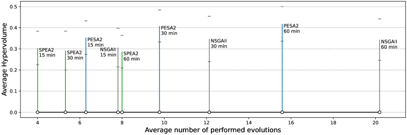
(a) TTBS

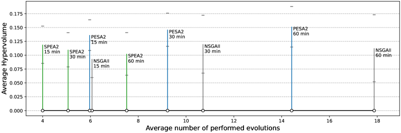
(b) CoCoME

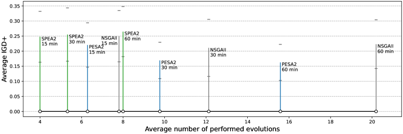
(c) TTBS

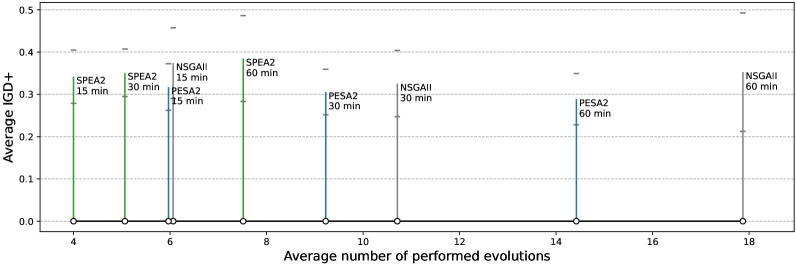
(d) CoCoME

Figure 2: Timelines of the number of evolutions performed by the algorithms for the different budget configurations, along with the achieved HV and IGD+. Vertical bars show the average HV and IGD+ over 30 runs, while ticks represent the standard deviation from the mean.

From the timelines, we can see that SPEA2 was the slowest algorithm in our experiments, whereas NSGA-II was the fastest one. Furthermore, for each search budget, NSGA-II performed the highest number of genetic evolutions, e.g., it performed on average $20$ genetic evolutions for TTBS with $60$ minutes of search budget, and almost $18$ genetic evolutions for CoCoME. Conversely, SPEA2 performed, on average, only $8$ evolutions for TTBS with a $60$ minutes search budget. Regarding PESA2, we can observe that it consistently generated the best QI in each case study and for every search budget. However, it turned out to be slower than NSGA-II, but faster than SPEA2.

It is worth mentioning that the two QIs showed the same behavior in the two case studies, therefore, for the sake of brevity, we only elaborate on observed behavior for HV. Analyzing the TTBS results, we observe that the HV values of SPEA2 almost lie close to $0.3$ for every search budget. For PESA2, in turn, the longer the search budget, the higher the HV values. The HV values for NSGA-II increase between the $15$ and $30$ minutes budgets and then become almost flat between $30$ and $60$ minutes. In addition, the timelines of the two case studies seemed to resemble each other. Also for CoCoME, NSGA-II was the fastest algorithm, SPEA2 the slowest one, and PESA2 generated the highest HV values. Furthermore, the number of genetic evolutions of CoCoME is consistent with that of TTBS.

Table 3 reports the results of the Mann–Whitney U test, and the corresponding $\hat{A}_{12}$ effect sizes. The name of the algorithm is underlined when i) the test resulted in a significant difference, and ii) that algorithm yielded high HV values. In this case, most tests revealed a significant difference between the algorithms in any given time budget (highlighted in bold). PESA2 performed best in many cases and in both case studies, NSGA-II scored best only in two cases in TTBS and not by a large margin, and SPEA2 was superior in the $15$ minutes budget test in CoCoME.

Budget	Algor. 1	Algor. 2	MWU p	$\hat{A}_{12}$
TTBS
15 min	PESA2	NSGA-II	0.0487	(S) 0.6462
15 min	SPEA2	NSGA-II	0.8548	(N) 0.486
15 min	SPEA2	PESA2	0.0234	(M) 0.3319
30 min	NSGA-II	PESA2	0.0167	(M) 0.3226
30 min	SPEA2	NSGA-II	0.0385	(S) 0.3465
30 min	SPEA2	PESA2	$<$0.0001	(L) 0.1582
60 min	NSGA-II	PESA2	0.0037	(M) 0.2851
60 min	SPEA2	NSGA-II	0.0202	(M) 0.3278
60 min	SPEA2	PESA2	$<$0.0001	(L) 0.1301
CoCoME
15 min	NSGA-II	SPEA2	0.0085	(M) 0.3049
15 min	PESA2	NSGA-II	0.0072	(M) 0.6993
15 min	PESA2	SPEA2	0.7999	(N) 0.4807
30 min	PESA2	NSGA-II	0.0066	(M) 0.7014
30 min	SPEA2	NSGA-II	0.5543	(N) 0.4558
30 min	SPEA2	PESA2	$<$0.0001	(L) 0.1738
60 min	PESA2	NSGA-II	0.0127	(M) 0.6847
60 min	SPEA2	NSGA-II	0.3789	(N) 0.4344
60 min	SPEA2	PESA2	$<$0.0001	(L) 0.1686

Table 3: Mann–Whitney U test and $\hat{A}_{12}$ effect sizes comparing the HV achieved by different algorithms in 30 runs. Magnitude interpretation: negligible (N), small (S), medium (M), large (L). The magnitude of the effect size is also represented by bars.

To investigate possible reasons behind such HV differences, we take a look at how the HV is achieved and when, by comparing it to the time budget and the number of performed evolutions.

Another viewpoint on the difference among the algorithms could be the actual quality of the computed solutions in terms of the non-functional properties of interest. To visually inspect this aspect, we relied on scatter plots comparing perfQ and reliability, because these objectives are the non-functional properties to be improved through the refactoring and optimization process. Along this line, Figures 3(a), 3(b) and 3(c) depict the three $PF^{c}$ when varying the time budget of all three genetic algorithms for both case studies. At a glance, we can observe a more densely populated $PF^{c}$ for CoCoME than for TTBS, while TTBS showed a more evident trend towards the top-right corner (the optimization direction for improving both objectives). Regarding the $PF^{c}$ for CoCoME, a horizontal clustering was observed for the three search budgets. The cluster that lies around $0.8$ for reliability is always more populated than the other two clusters: one between $0.4$ and $0.6$, and the other between $0.0$ and $0.2$, approximately. There is not an evident motivation for the horizontal clustering of CoCoME. We conjecture that the characteristics of the CoCoME model, which has a more complex behavior than TTBS, prevent the algorithms from reaching higher reliability values for the search budgets we considered. Also, the CoCoME solution space seems to be less homogeneous, with feasible solutions that are inherently clustered.

In summary, we can answer RQ1 by saying that there is a clear difference among the algorithms when comparing them on the basis of a QI for multi-objective optimization, like the HV, and when pursuing speed in completing evolutions as the main goal of the designer. Nonetheless, if we only look at the non-functional properties of the optimization, the shape of the $PF^{c}$ and the explored design space do not differ much from those covered by the $PF^{ref}$.

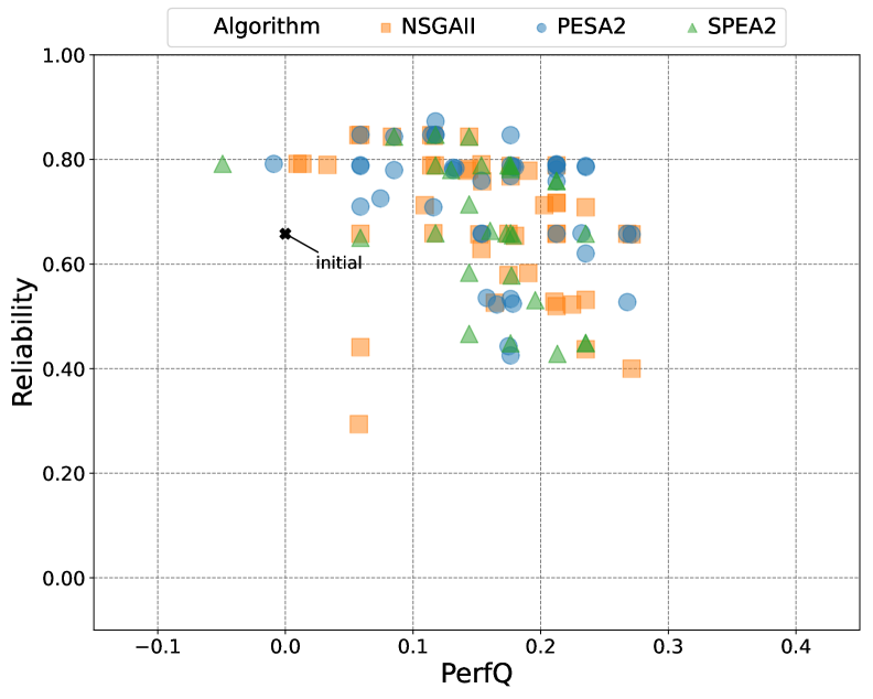
TTBS CoCoME

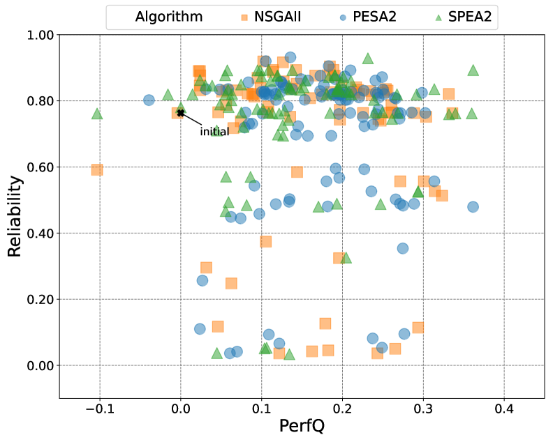
(a) 15 min budget

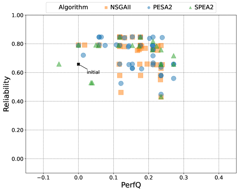
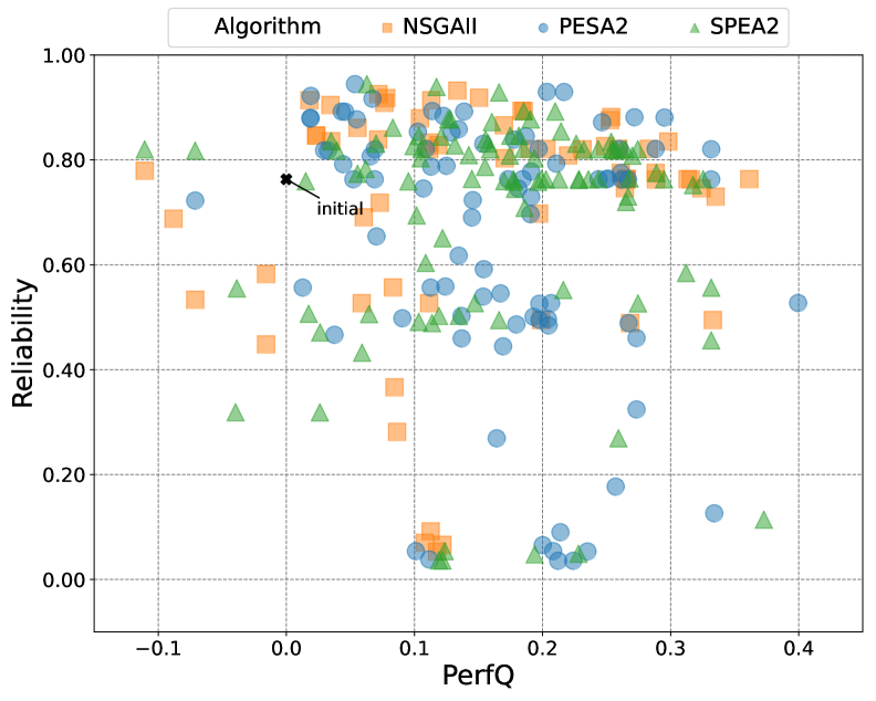
(b) 30 min budget

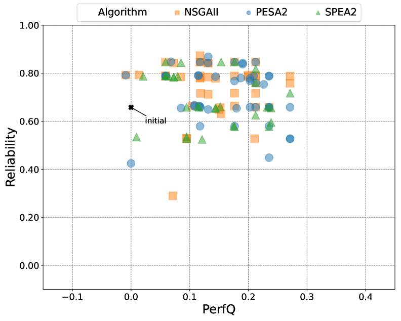
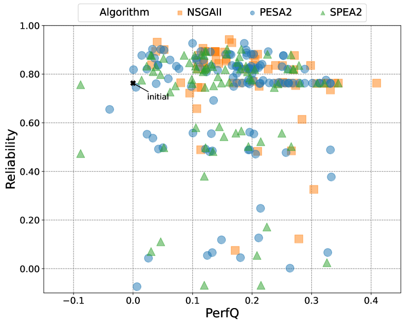
(c) 60 min budget

Figure 3: TTBS and CoCoME Pareto frontiers for perfQ and reliability obtained by the three algorithms when varying the time budget between 15, 30, and 60 minutes. The top-right corner is the optimal point, whereas the bottom-left corner is the worst one. Filled symbols correspond to the results of each algorithm

6.2 RQ2: To what extent does the time budget affect the quality of Pareto fronts?

The first main concern about imposing a search budget is its effect on the optimization process. We remark that we analyze the HV only (as already discussed in Section 6.1) since the two considered QIs showed quite the same behavior. Table 4 reports, for each algorithm and search budget, the average HV achieved in 30 runs along with its standard deviation. Intuitively, this indicator gives an idea of how much of the solution space was covered with the budget restriction, compared to a run without restrictions. We can observe that, in fact, the time budget affects the quality of the computed Pareto fronts.

Algor.	Budget	HV avg	HV stdev
TTBS ($\Omega=1.2\times 10^{13}$)
NSGA-II	15 min	0.3060	0.0915
NSGA-II	30 min	0.3469	0.1071
NSGA-II	60 min	0.3437	0.0980
PESA2	15 min	0.3532	0.0794
PESA2	30 min	0.4084	0.0757
PESA2	60 min	0.4182	0.0819
SPEA2	15 min	0.3041	0.0794
SPEA2	30 min	0.2917	0.0920
SPEA2	60 min	0.2868	0.0769
CoCoME ($\Omega=3.26\times 10^{16}$)
NSGA-II	15 min	0.0931	0.0335
NSGA-II	30 min	0.1199	0.0523
NSGA-II	60 min	0.1125	0.0604
PESA2	15 min	0.1363	0.0277
PESA2	30 min	0.1460	0.0300
PESA2	60 min	0.1514	0.0366
SPEA2	15 min	0.1189	0.0336
SPEA2	30 min	0.1098	0.0309
SPEA2	60 min	0.1023	0.0384

Table 4: Average HV quality indicator and its standard deviation over 31 runs, listed by algorithm and search budget. Higher values are associated to a better quality of the Pareto fronts. $\Omega$ is the size of the solution space computed as the Cartesian product of the types of refactoring actions and all the eligible refactoring targets in any possible refactoring sequence.

The search budget had a different impact on the two case studies. In TTBS, the search was able to achieve a better HV in all cases, when compared to that of CoCoME. This is probably due to the difference in size and complexity between the two case studies. CoCoME permits a larger number of possible refactoring candidates, and its model defines a more complex behavior. These factors inherently lead to a bigger search space ($\Omega$ in the table), but also to spend more time in computing the objective functions. Therefore, on average, the longer it takes to complete a single evolution, the fewer evolutions will be performed for a given time budget.

To assess whether doubling or quadrupling the time budget makes a significant difference in the HV of the $PF^{c}$, we compare the results obtained with different budgets but with the same algorithm. Table 5 reports the results of the Mann–Whitney U test and the corresponding $\hat{A}_{12}$ effect size. The p-value is highlighted in bold when the detected difference is statistically significant. The time budget is underlined when i) the test showed a significant difference, and ii) the experiment running on that time budget led to higher HV values. In very few cases (two per case study), we obtained a significant difference, and in all the cases this trend was detected for PESA2: with a medium magnitude in TTBS and a large one in CoCoME. This situation suggests that, except for PESA2, the main difference in the HV values might be attributed to a difference in the algorithm being used, rather than to a difference in the budget. We further investigate this aspect in the next section.

In summary, RQ2 indicates that the time budget is closely linked to the complexity and topology of the system under analysis. We discovered that the number of genetic evolutions is related to the time needed to compute the non-functional indices (performance and reliability), which is longer when the system is more complex.

Algor.	Budget 1	Budget 2	MWU p	$\hat{A}_{12}$
TTBS
NSGA-II	15 min	30 min	0.1677	(S) 0.3975
NSGA-II	15 min	60 min	0.1677	(S) 0.3975
NSGA-II	30 min	60 min	0.9327	(N) 0.5068
PESA2	15 min	30 min	0.018	(M) 0.3247
PESA2	15 min	60 min	0.0031	(M) 0.281
PESA2	30 min	60 min	0.4223	(N) 0.4402
SPEA2	15 min	60 min	0.4992	(N) 0.5505
SPEA2	30 min	15 min	0.4556	(N) 0.4443
SPEA2	30 min	60 min	0.7999	(N) 0.4807
CoCoME
NSGA-II	15 min	30 min	0.0574	(S) 0.359
NSGA-II	60 min	15 min	0.1054	(S) 0.6202
NSGA-II	60 min	30 min	0.8769	(N) 0.488
PESA2	15 min	30 min	$<$0.0001	(L) 0.2092
PESA2	60 min	15 min	$<$0.0001	(L) 0.7992
PESA2	60 min	30 min	0.6024	(N) 0.539
SPEA2	30 min	15 min	0.2483	(S) 0.4142
SPEA2	60 min	15 min	0.1249	(S) 0.3861
SPEA2	60 min	30 min	0.6123	(N) 0.462

Table 5: Mann–Whitney U test and $\hat{A}_{12}$ effect sizes comparing the HV achieved with different time budgets in 30 runs. Magnitude interpretation: negligible (N), small (S), medium (M), large (L). The magnitude of the effect size is also represented by bars.

6.3 RQ3: Do different time budgets generate different software models?

For an initial assessment of the kinds of software models resulting from the time budgets, we generated scatter plots for #changes and #pas objectives as depicted in Figure 4. We observed that the solutions were confined to compact, well-defined regions of the space, in contrast to the variety of solutions offered by the reference Pareto front. In both case studies, two main clusters of solutions were identified. The clusters were very clear (and segregated) in TTBS, with the majority of the models having at most one antipattern, and their refactoring costs were in a mid-range ($[3-25]$). For CoCoME, the clusters shared some boundaries. The refactoring cost was around the same range as for TTBS, while the number of antipatterns covered an extended range and had more variability ($[2-13]$).

The patterns for the clusters were similar, regardless of the algorithm being used. Some exceptions were noticed for NSGA-II, particularly for CoCoME, with more dispersed solutions than PESA2 and SPEA2. Restricting the time budget led to models with relatively few variations in terms of refactoring cost and antipatterns. Although there were slight differences in the CoCoME results, increasing the time budget did seem to affect the general cluster patterns. This means that even when imposing a time budget, the designer has chances of finding a number of (Pareto) optimal solutions for the refactoring problem. Certainly, the corresponding (alternative) models will be fewer (in terms of #changes and #pas) than when running the algorithms with no budgets.

It should be noticed that #changes and #pas provide a limited characterization of the underlying software models, as other structural properties of the models are not captured. For example, two models having one antipattern and a refactoring cost of $10$ might still differ in their design structure. Thus, a finer-grained characterization of the models can help to expose additional differences. We elaborate on this issue to answer the RQ4, described in Section 6.4.

In summary, we can answer RQ3 by saying that the usage of time budgets leads to a restricted set of design alternatives, but some of them are Pareto optimal. The different budgets seem to produce similar models, and only NSGA-II was able to generate a slightly wider range of alternatives than the remaining algorithms.

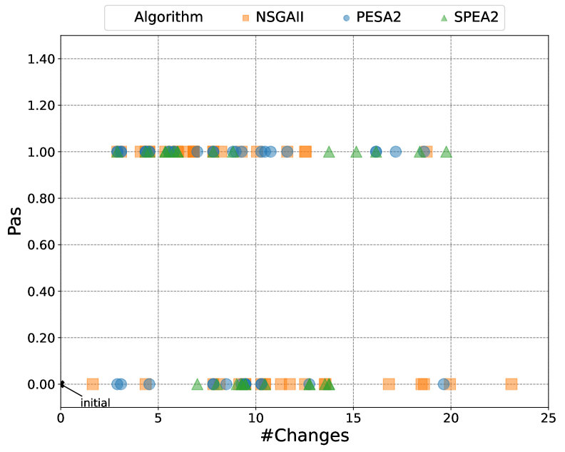
TTBS CoCoME

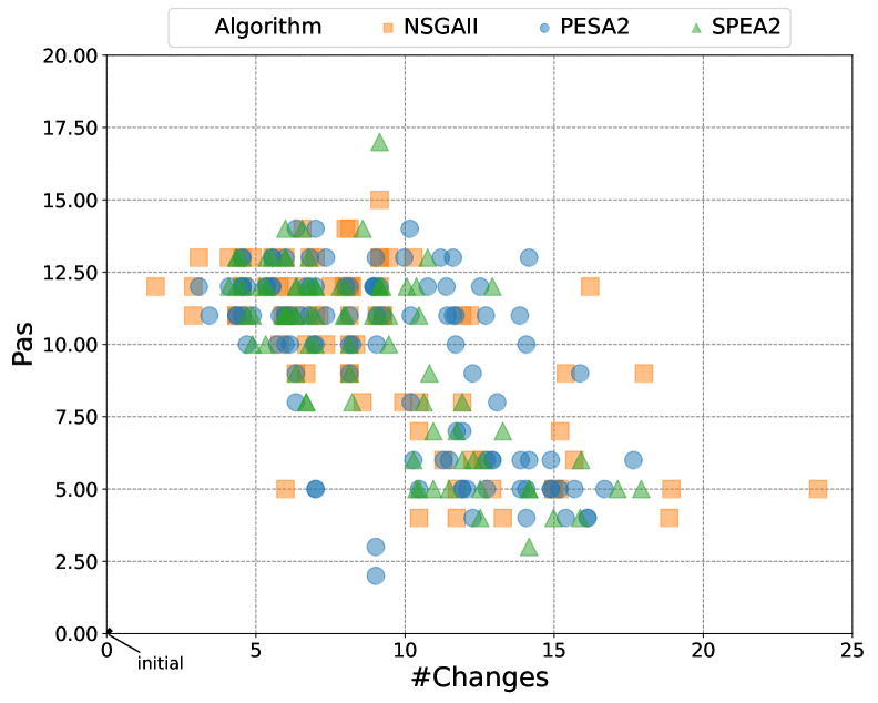
(a) 15 min budget

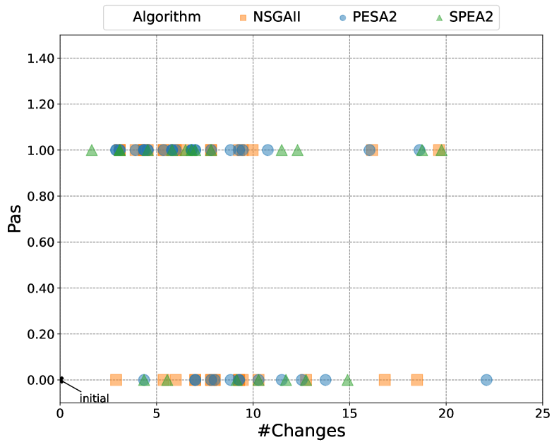
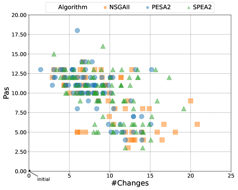
(b) 30 min budget

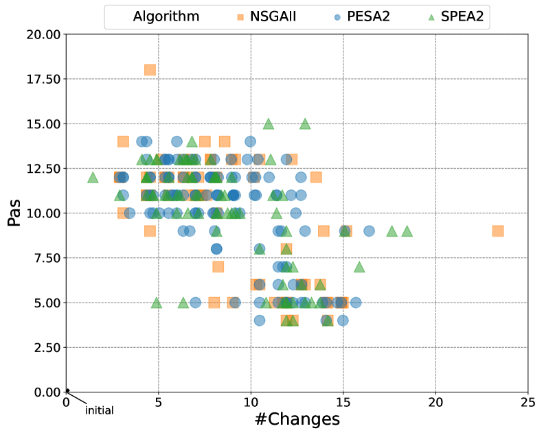
(c) 60 min budget

Figure 4: TTBS and CoCoME Pareto frontiers for #changes and #pas obtained by the three algorithms when varying the time budget between 15, 30, and 60 minutes. The bottom-left corner is the optimal point, whereas the top-right corner is the worst one. Filled symbols correspond to the results of each algorithm.

6.4 RQ4: How do the sequences of refactoring actions look like when using different budgets?

From a constructive (or structural) point of view, the software models result from applying (sequences of) refactoring actions on the initial software model. Altogether, these refactoring actions constitute the search space explored by a given algorithm. In this context, one could take all the refactoring sequences used in a given experiment and arrange them as a prefix tree, in which the leaves correspond to models and the inner nodes capture actions shared by the different sequences. This tree representation is useful for identifying unique sequences in a given search space, but also for computing sequence intersections between the trees coming from different algorithms or budgets.

For instance, Figure 5 and Figure 6 show a pair of trees for certain TTBS and CoCoME experiments, respectively. Each path from the root to a leaf represents a unique sequence of refactoring actions, which can produce one or more models. All the sequences involve exactly four refactoring actions. The colored paths correspond to common sequences (i.e., an intersection) between both trees, while the remaining paths are particular to each tree. In this way, we can (approximately) determine that using a 30 min time budget (either for TTBS or CoCoME) generates a subset of models that are structurally different from those generated by running the optimization without any time budget ($PF^{ref}$). Note also that the number of unique sequences in $PF^{ref}$ is smaller (i.e., less diverse) than that of the space explored with a time budget. Our idea with the these trees is to establish a “profile” of refactoring actions for a given experiment, and then make comparisons with other profiles. In general, the representation and analysis of search spaces have received less attention in the architecture optimization literature, since most works have focused on the objective space.

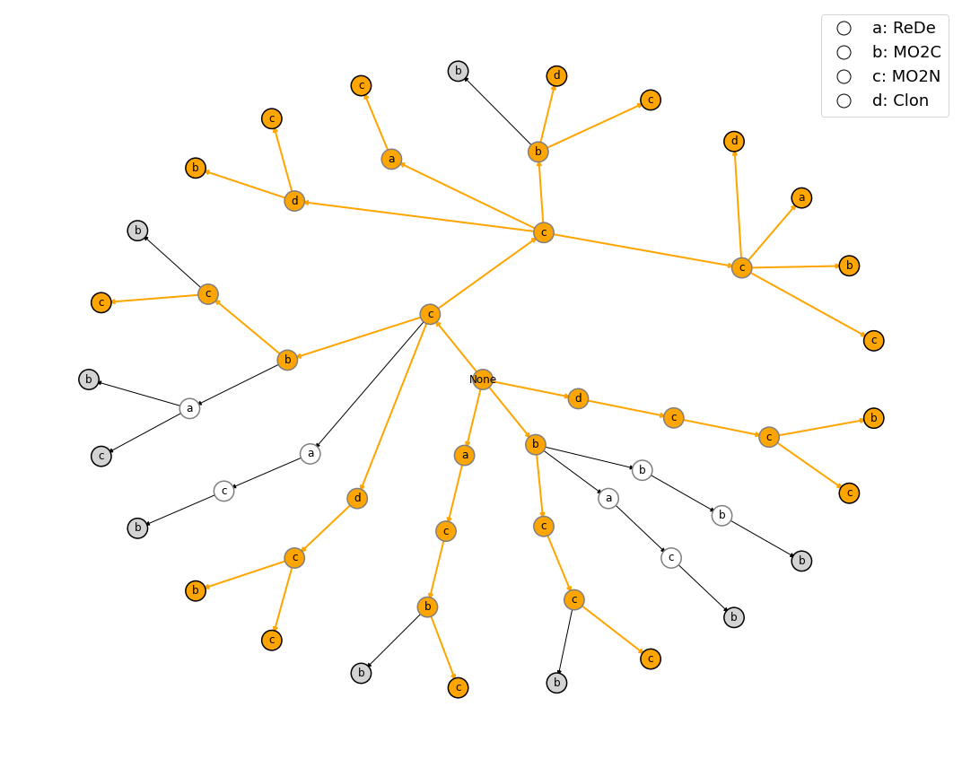
(a) baseline ($PF^{ref}$) - TTBS

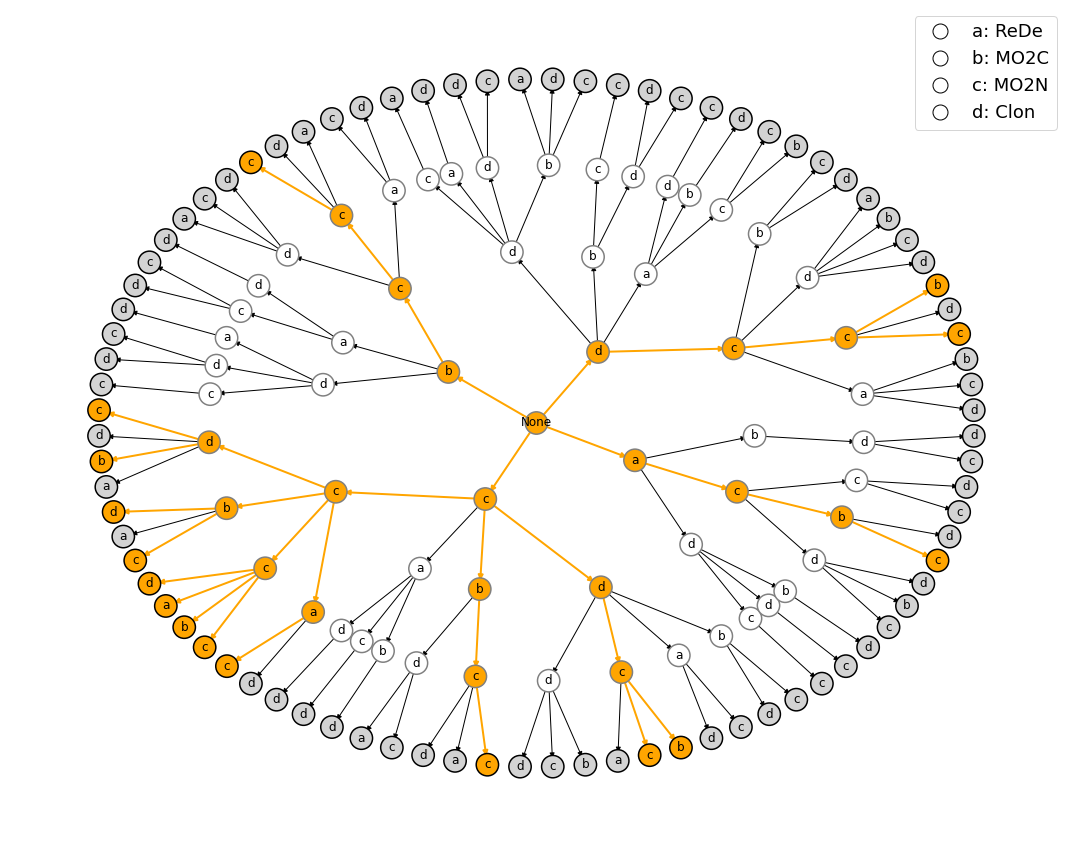
(b) 30 min budget - TTBS

Figure 5: Examples of search spaces for TTBS represented as trees, as generated by NSGA-II. The orange nodes and edges are sequences of refactoring actions shared by both trees (i.e., intersections). Each node maps to an individual refactoring action as indicated in the legend.

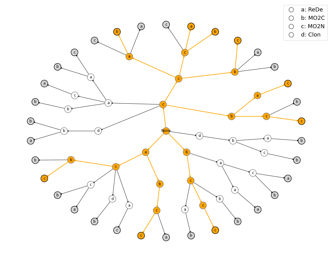
(a) baseline ($PF^{ref}$) - CoCoME

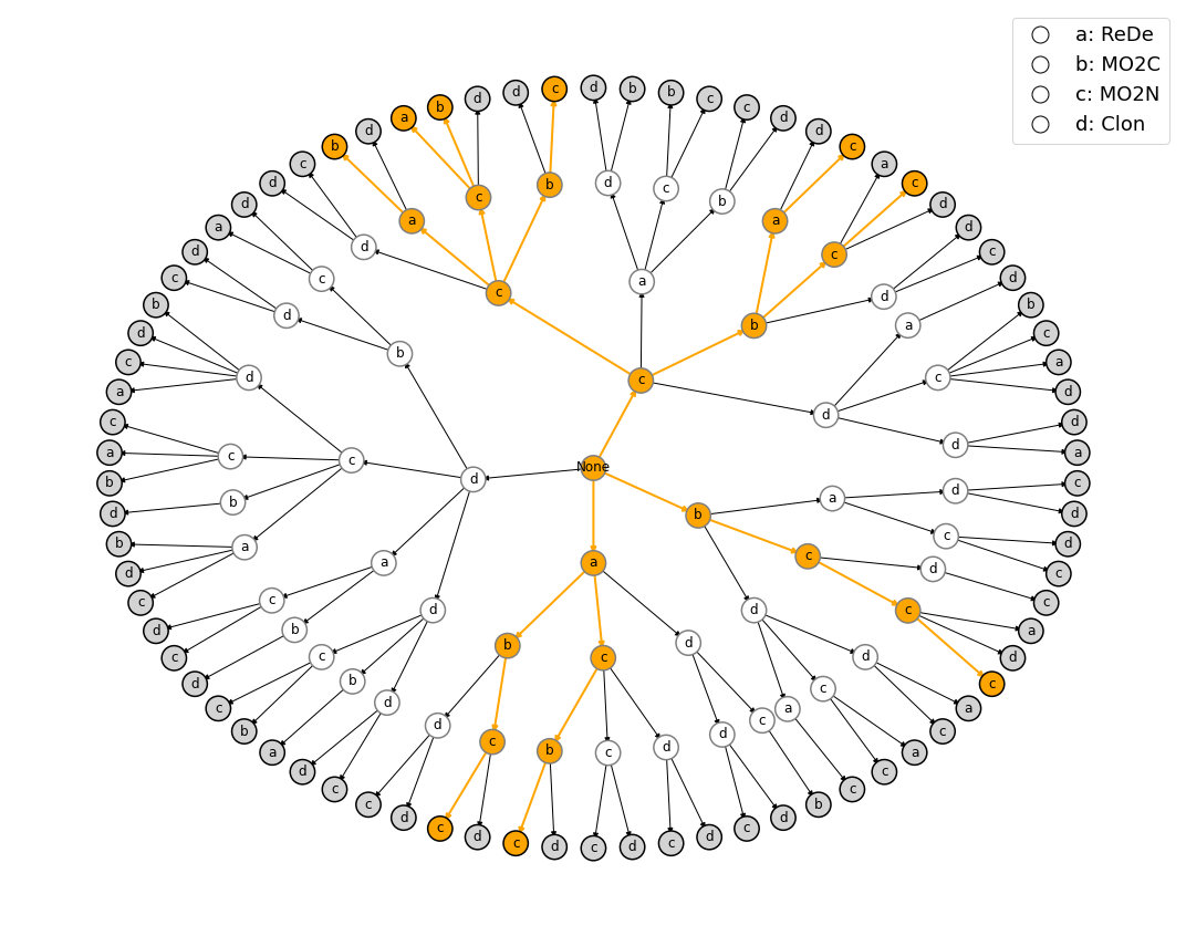
(b) 30 min budget - CoCoME

Figure 6: Examples of search spaces for CoCoME represented as trees, as generated by NSGA-II. The orange nodes and edges are sequences of refactoring actions shared by both trees (i.e., intersections). Each node maps to an individual refactoring action, as indicated in the legend.

According to the procedure exemplified above, we compared the sequence trees obtained with different budgets among themselves and also compared each tree against the tree for $PF^{ref}$ (baseline). For TTBS, we found that between $18-37\%$ of the sequences obtained with time budgets were shared by the $PF^{ref}$. These percentages were in the range $8-24\%$ for CoCoME. These numbers would indicate that more than half of the models generated when using budgets differ from those found in the $PF^{ref}$. As for the intersection of the trees resulting from imposing each budget, we observed an average of $25\%$ of shared sequences for CoCoME and variations between $33\%$ and $51\%$ for TTBS, but without a clear trend with respect to the choice of the algorithms. These results are aligned with the observations made for the scatter plots in Figure 4, indicating that using limited time budgets does not produce many different models.

Regarding the $PF^{ref}$, nonetheless, the trees resulting from the time budgets included many more sequences (in terms of types of refactoring actions) than the baseline trees. This was a common trend for both case studies, as hinted by Figure 5 and Figure 6, in which the trees on the right are more dense than the trees on the left. We believe this situation is due to the convergence of the solutions (and the corresponding sequences thereof) near the Pareto front, after a considerable number of evolutions.

To further analyze differences in the software models, we computed the frequency of the refactoring actions being used by the sequences in the experiments. The intuition here is that the repeated usage of certain actions might be driven by the optimization objectives, which might originate the model differences within a given search space. The (normalized) frequency for the four available actions for CoCoME and TTBS is summarized in Figure 7. Note that every sequence consists of exactly four actions.

For CoCoME, we can see that the frequency of actions resulting from imposing the budgets are more or less similar in their composition, with MO2N being on par with Clon as the most prevalent actions. This pattern contrasts with the very high frequency of MO2N observed in the baselines and the very low contributions of the remaining actions. We conjecture that this action could play a key role in the solutions in the $PF^{ref}$, and this might explain why some solutions in the experiments using time budgets did not reach the Pareto front. The frequencies for the baselines achieved by the three algorithms also showed some variations, such as the prevalence of MO2C for NSGA-II in the fourth sequence position. When it comes to TTBS, the patterns were similar to those for CoCoME, but the prevalence of MO2N was even higher in the baselines, except for PESA2 where that action was less dominant and other actions were used. In addition, MO2C became more relevant in the fourth sequence position for PESA2 and NSGA-II, as in the case of CoCoME. This could hint at a particular behavior in the last sequence position mainly for NSGA-II.

In general, we observe that the frequency profiles provide additional evidence about the similarity among the models generated with the time budgets, as well as their differences with respect to the models in $PF^{ref}$. The high-prevalence pattern for a specific action (such as MO2N) and the role of actions in the last sequence position could be related to the satisfaction of the optimization objectives (within the algorithms), although the phenomenon should still be further studied.

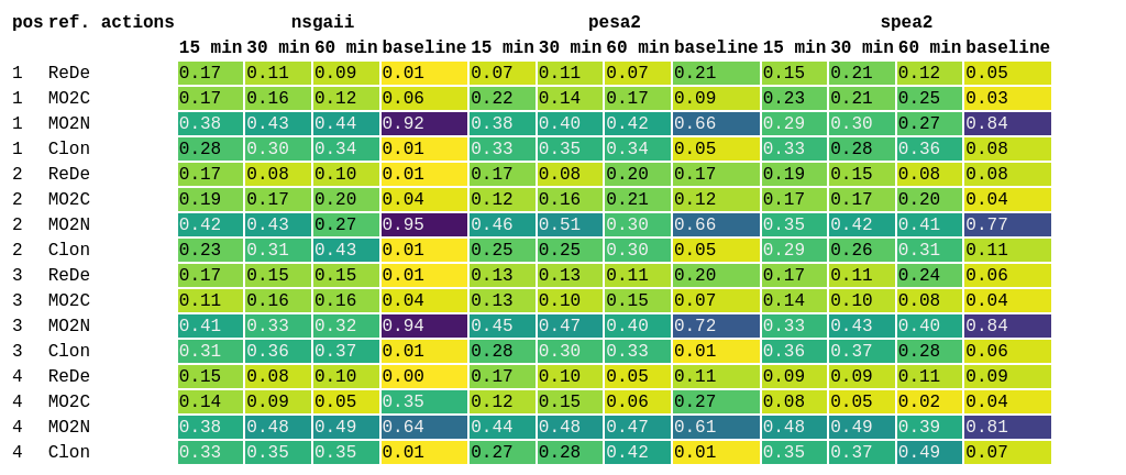
(a) TTBS

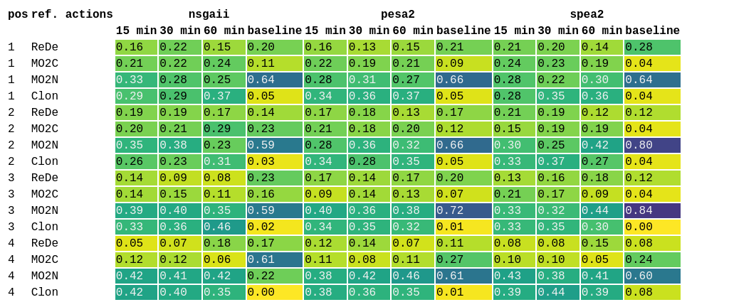
(b) CoCoME

Figure 7: Frequency of refactoring actions used at each position of the sequences, for different time budgets and algorithms. The sequence position is indicated by the pos column.

Overall, we can answer RQ4 by saying that using time budgets generates different models, in terms of sequences of refactoring actions, while sharing a small fraction of those models with $PF^{ref}$. This fraction did seem to be affected by increases in the budget. The search spaces derived from the budgets tend to have many models in common, with some variations that could be attributed to the policies of each algorithm. The profiles of refactoring actions were also similar, regardless of the time budgets or algorithms being used,

7 Threats to validity

In this section, we discuss threats that might affect our results.

Construct validity

An aspect that might affect our results is the estimation of the reference Pareto front ($PF^{ref}$), which is used to extract the quality indicators, as described in Section 4. We mitigate this threat by building the $PF^{ref}$ from a run without a search budget for each case study. Therefore, $PF^{ref}$ should contain all the non-dominated solutions across all configurations, and it should also represent a good Pareto front for computing the HV and IGD+ indicators.

Another important aspect that might threaten our experimentation concerns the parameters of the initial UML model. For example, CoCoME showed higher initial reliability that might affect the search. However, in our experiments, it seems that TTBS and CoCoME initial configurations did not threaten the optimization process. We will further investigate how different initial UML model parameters could change the optimization results. We remark that changing a single model parameter means starting the optimization process on a different point of the solution space that might produce completely different results.

External validity

Our results might be affected by external validity threats, as their generalization might be limited to some of the assumptions behind our approach.

In the first place, a threat might be represented by the use of a single modeling notation. We cannot generalize our results to other modeling notations, which could imply using a different portfolio of refactoring actions. The syntax and semantics of the modeling notation determine the amount and nature of refactoring actions that can be performed. However, we have adopted UML, which is the de facto standard in the software modeling domain. In general terms, this threat can be mitigated by porting the whole approach on a different modeling notation, but this is out of this paper scope.

Another threat might be found in the fact that we have validated our approach on two case studies. While the two case studies were selected from the available literature, they might not represent all the possible challenges that our approach could face in practice.

Internal validity

Our optimization approach might be affected by internal validity threats. There are high degrees of freedom on our settings. For example, the variations of genetic configurations, such as the $P_{crossover}$ probability, may produce $PF^{c}$ with different quality solutions. Also, the problem configuration variations may also change our results. The degrees of freedom in our experimentation generate unfeasible brute force investigation of each suitable combination. For this reason, we limit the variability to subsets of problem configurations, as shown in Table 1. We also mitigate this threat by involving two different case studies derived from the literature, thus reducing biases in their construction.

Another aspect that might affect our findings is a misleading interpretation of the outcome due to the random nature of genetic algorithms. In order to mitigate this threat, we performed 30 executions for each configuration [44].

Conclusion validity

The observations made by this study might change with different, better-tuned parameters for each algorithm. For scoping reasons, we did not perform an extensive tuning phase for each algorithm. Instead, we rely on common parameters to set up the algorithms, which should mitigate the threat [50]. Wherever possible, we used appropriate statistical procedures with p-value and effect size measures to test the significance of the differences and their magnitude.

Another aspect that might affect our results is the estimation of the reference Pareto frontier ($PF^{ref}$). $PF^{ref}$ is used for extracting the quality indicators as described in Section 6. We soften this threat by building the $PF^{ref}$ overall our $PF^{c}$ for each case study. Therefore, the reference Pareto should optimistically contain all non-dominated solutions across all configurations.

8 Conclusion and Future Work

In this study, we presented an investigation of the impact of the time budget for multi-objective refactoring optimization of software models. The study aims at helping designers to select the best algorithm with respect to the time budget. We performed the study on two model benchmarks, Train Ticket Booking Service, and CoCoME, and on three genetic algorithms, NSGA-II, SPEA2, and PESA2.

We assessed the quality of the results obtained by each algorithm through the HV and IGD+ indicators. HV measures the amount of the search space volume that a computed Pareto front ($PF^{c}$) covers with respect to a reference Pareto front ($PF^{ref}$), while IGD+ is the inverse of the Euclidean distance between points belonging to $PF^{c}$ and $PF^{ref}$. From our results (see Section 6.1, and Section 6.2), NSGA-II emerged as the fastest algorithm because it performed the highest number of genetic evolutions within the search budget. PESA2, in turn, was the algorithm that generated the best quality results in terms of HV. SPEA2 was the slowest algorithm and generated the results with the worst quality. This means that it achieved the lowest number of genetic evolutions and the lowest HV values.

Regarding the different budgets, they seem to produce similar models both in terms of structure and objective values, and only NSGA-II was able to generate a slightly wider range of alternatives than the remaining algorithms (see Section 6.3 and Section 6.4). In terms of their sequences of refactoring actions, the sets of models derived from the time budgets tend to have many models in common, despite some variations attributed to the policies of each algorithm. Moreover, a small fraction of these models was shared with those models in $PF^{ref}$, which indicate that the budgets can still generate optimal models.

As future work, also with the goal of saving optimization time, we intend to analyze the Pareto front at each evolution in order to detect situations in which the quality is not having enough improvement, and one could decide to stop the algorithm. Furthermore, we would like to get more insights from the tree representation of the search spaces, which can enable the discovery of particular refactoring actions being correlated with the satisfaction of certain objectives by the optimization algorithms. Finally, we plan to experiment with additional case studies and further investigate the impact of the case study structure (i.e., size and complexity) on the quality of the optimization results.

References

- Ramírez et al. [2019] A. Ramírez, J. R. Romero, S. Ventura, A survey of many-objective optimisation in search-based software engineering, Journal of Systems and Software 149 (2019) 382–395. doi:10.1016/j.jss.2018.12.015.
- Bavota et al. [2014] G. Bavota, M. Di Penta, R. Oliveto, Search Based Software Maintenance: Methods and Tools, Springer Berlin Heidelberg, Berlin, Heidelberg, 2014, p. 103–137. URL: http://link.springer.com/10.1007/978-3-642-45398-4_4. doi:10.1007/978-3-642-45398-4_4.