Symbolic ltl_f Best-Effort Synthesis

Abstract

We consider an agent acting to fulfil tasks in a nondeterministic environment. When a strategy that fulfills the task regardless of how the environment acts does not exist, the agent should at least avoid adopting strategies that prevent from fulfilling its task. Best-effort synthesis captures this intuition. In this paper, we devise and compare various symbolic approaches for best-effort synthesis in Linear Temporal Logic on finite traces (ltl_f). These approaches are based on the same basic components, however they change in how these components are combined, and this has a significant impact on the performance of the approaches as confirmed by our empirical evaluations.

1 Introduction

We consider an agent acting to fulfill tasks in a nondeterministic environment, as considered in Planning in nondeterministic (adversarial) domains [8, 15], except that we specify both the environment and the task in Linear Temporal Logic (ltl) [3], the formalism typically used for specifying complex dynamic properties in Formal Methods [5].

In fact, we consider Linear Temporal Logic on finite traces (ltl_f) [11, 12], which maintains the syntax of ltl [18] but is interpreted on finite traces. In this setting, we study synthesis [17, 13, 12, 3]. In particular, we look at how to synthesize a strategy that is guaranteed to satisfy the task against all environment behaviors that conform to the environment specification.

When a winning strategy that fulfills the agent’s task, regardless of how the environment acts, does not exist, the agent should at least avoid adopting strategies that prevent it from fulfilling its task. Best-effort synthesis captures this intuition. More precisely, best-effort synthesis captures the game-theoretic rationality principle that a player would not use a strategy that is “dominated” by another of its strategies (i.e. if the other strategy would fulfill the task against more environment behaviors than the one chosen by the player). Best-effort strategies have been studied in [4] and proven to have some notable properties: (i) they always exist, (ii) if a winning strategy exists, then best-effort strategies are exactly the winning strategies, (iii) best-effort strategies can be computed in 2EXPTIME as computing winning strategies (best-effort synthesis is indeed 2EXPTIME-complete).

The algorithms for best-effort synthesis in ltl and ltl_f have been presented in [4]. These algorithms are based on creating, solving, and combining the solutions of three distinct games but of the same game arena. The arena is obtained from the automata corresponding to the formulas $\mathcal{E}$ and $\varphi$ constituting the environment and the task specifications, respectively.

In particular, the algorithm for ltl_f best-effort synthesis appears to be quite promising in practice since well-performing techniques for each component of the algorithm are available in the literature. These components are: (i) transformation of the ltl_f formulas $\mathcal{E}$ and $\varphi$ into deterministic finite automata (dfa), which can be double-exponential in the worst case, but for which various good techniques have been developed [16, 22, 6, 10]; (ii) Cartesian product of dfas, which is polynomial; (iii) minimization of dfas, which is also polynomial; (iv) fixpoint computation over dfa to compute adversarial and cooperative winning strategies for reaching the final states, which is again polynomial.

In this paper, we refine the ltl_f best-effort synthesis techniques presented in [4] by using symbolic techniques [7, 5, 22]. In particular, we show three different symbolic approaches that combine the above operations in different ways (and in fact allow for different levels of minimization). We then compare the three approaches through empirical evaluations. From this comparison, a clear winner emerges. Interestingly, the winner does not fully exploit dfa minimization to minimize the dfa whenever it is possible. Instead, this approach uses uniformly the same arena for all three games (hence giving up on minimization at some level). Finally, it turns out that the winner performs better in computing best-effort solutions even than state-of-the-art tools that compute only adversarial solutions. These findings confirm that ltl_f best-effort synthesis is indeed well suited for efficient and scalable implementations.

The rest of the paper is organized as follows. In Section 2, we recall the main notions of ltl_f synthesis. In Section 3, we discuss ltl_f best-effort synthesis, and the algorithm presented in [4]. In Section 4, we introduce three distinct symbolic approaches for ltl_f best-effort synthesis: the first (c.f., Subsection 4.2) is a direct symbolic implementation of the algorithm presented in [4]; the second one (c.f., Subsection 4.3) favors maximally conducting dfa minimization, thus getting the smallest possible arenas for the three games; and the third one (c.f., Subsection 4.4) gives up dfa minimization at some level, and creates a single arena for the three games. In Section 5, we perform an empirical evaluation of the three algorithms. We conclude the paper in Section 6.

2 Preliminaries

ltl_f Basics.

Linear Temporal Logic on finite traces (ltl_f) is a specification language to express temporal properties on finite traces [11]. In particular, ltl_f has the same syntax as ltl, which is instead interpreted over infinite traces [18]. Given a set of propositions $\Sigma$, ltl_f formulas are generated as follows:

$$\varphi::=a\mid(\varphi_{1}\wedge\varphi_{2})\mid(\neg\varphi)\mid(\raisebox{-1.1625pt}{\LARGE$\circ$}\varphi)\mid(\varphi_{1}\mathop{\mathcal{U}}\varphi_{2})$$

where $a\in\Sigma$ is an atom, $\circ$ (Next), and $\mathop{\mathcal{U}}$ (Until) are temporal operators. We make use of standard Boolean abbreviations such as $\vee$ (or) and $\rightarrow$ (implies), $\mathit{true}$ and $\mathit{false}$. In addition, we define the following abbreviations Weak Next $\raisebox{-1.1625pt}{\LARGE$\bullet$}\varphi\equiv\neg\raisebox{-1.1625pt}{\LARGE$\circ$}\neg\varphi$, Eventually $\Diamond\varphi\equiv\mathit{true}\mathop{\mathcal{U}}\varphi$ and Always $\Box\varphi\equiv\neg\Diamond\neg\varphi$. The length/size of $\varphi$, written $|\varphi|$, is the number of operators in $\varphi$.

A finite (resp. infinite) trace is a sequence of propositional interpretations $\pi\in(2^{\Sigma})^{*}$ (resp. $\pi\in(2^{\Sigma})^{\omega}$). For every $i\geq 0$, $\pi_{i}\in 2^{\Sigma}$ is the $i$-th interpretation of $\pi$. Given a finite trace $\pi$, we denote its last instant (i.e., index) by ${\sf{lst}}(\pi)$. ltl_f formulas are interpreted over finite, nonempty traces. Given a finite, non-empty trace $\pi\in(2^{\Sigma})^{+}$, we define when an ltl_f formula $\varphi$ holds at instant $i$, $0\leq i\leq{\sf{lst}}(\pi)$, written $\pi,i\models\varphi$, inductively on the structure of $\varphi$, as:

• $\pi,i\models a\text{ iff }a\in\pi_{i}$ (for $a\in{\Sigma}$);

• $\pi,i\models\lnot\varphi\text{ iff }\pi,i\not\models\varphi$;

• $\pi,i\models\varphi_{1}\wedge\varphi_{2}\text{ iff }\pi,i\models\varphi_{1}\text{ and }\pi,i\models\varphi_{2}$;

• $\pi,i\models\raisebox{-1.1625pt}{\LARGE$\circ$}\varphi\text{ iff }i<{\sf{lst}}(\pi)$ and $\pi,i+1\models\varphi$;

• $\pi,i\models\varphi_{1}\mathop{\mathcal{U}}\varphi_{2}$ iff $\exists j$ such that $i\leq j\leq{\sf{lst}}(\pi)$ and $\pi,j\models\varphi_{2}$, and $\forall k,i\leq k<j$ we have that $\pi,k\models\varphi_{1}$.

We say $\pi$ satisfies $\varphi$, written as $\pi\models\varphi$, if $\pi,0\models\varphi$.

Reactive Synthesis Under Environment Specifications.

Reactive synthesis concerns computing a strategy that allows the agent to achieve its goal in an adversarial environment. In many AI applications, the agent has a model describing possible environment behaviors, which we call here an environment specification [2, 3]. In this work, we specify both environment specifications and agent goals as ltl_f formulas defined over $\Sigma=\mathcal{X}\cup\mathcal{Y}$, where $\mathcal{X}$ and $\mathcal{Y}$ are disjoint sets of variables under the control of the environment and the agent, respectively.

An agent strategy is a function $\sigma_{ag}:(2^{\mathcal{X}})^{*}\rightarrow 2^{\mathcal{Y}}$ that maps a sequence of environment choices to an agent choice. Similarly, an environment strategy is a function $\sigma_{env}:(2^{\mathcal{Y}})^{+}\rightarrow 2^{\mathcal{X}}$ mapping non-empty sequences of agent choices to an environment choice. A trace $\pi=(X_{0}\cup Y_{0})(X_{1}\cup Y_{1})\ldots\in(2^{\mathcal{X}\cup\mathcal{Y}})^{\omega}$ is $\sigma_{ag}$-consistent if $Y_{0}=\sigma_{ag}(\epsilon)$, where $\epsilon$ denotes empty sequence, and $Y_{i}=\sigma_{ag}(X_{0},\ldots,X_{i-1})$ for every $i>0$. Analogously, $\pi$ is $\sigma_{env}$-consistent if $X_{i}=\sigma_{env}(Y_{0},\ldots,Y_{i})$ for every $i\geq 0$. We define $\pi(\sigma_{ag},\sigma_{env})$ to be the unique infinite trace that is consistent with both $\sigma_{ag}$ and $\sigma_{env}$.

Let $\psi$ be an ltl_f formula over $\mathcal{X}\cup\mathcal{Y}$. We say that agent strategy $\sigma_{ag}$ enforces $\psi$, written $\sigma_{ag}\triangleright\psi$, if for every environment strategy $\sigma_{env}$, there exists a finite prefix of $\pi(\sigma_{ag},\sigma_{env})$ that satisfies $\psi$. Conversely, we say that an environment strategy $\sigma_{env}$ enforces $\psi$, written $\sigma_{env}\triangleright\psi$, if for every agent strategy $\sigma_{ag}$, every finite prefix of $\pi(\sigma_{ag},\sigma_{env})$ satisfies $\psi$. $\psi$ is agent enforceable (resp. environment enforceable) if there exists an agent (resp. environment) strategy that enforces it. An environment specification is an ltl_f formula $\mathcal{E}$ that is environment enforceable.

The problem of ltl_f reactive synthesis under environment specifications is defined as follows.

Definition 1

The ltl_f reactive synthesis under environment specifications problem is defined as a pair $\mathcal{P}=(\mathcal{E},\varphi)$, where ltl_f formulas $\mathcal{E}$ and $\varphi$ correspond to an environment specification and an agent goal, respectively. Realizability of $\mathcal{P}$ checks whether there exists an agent strategy $\sigma_{ag}$ that enforces $\varphi$ under $\mathcal{E}$, i.e.,

$$\forall\sigma_{env}\triangleright\mathcal{E},\pi(\sigma_{ag},\sigma_{env})\models\varphi$$

Synthesis of $\mathcal{P}$ computes such a strategy if it exists.

A naive approach to this problem is a reduction to standard reactive synthesis of ltl_f formula $\mathcal{E}\rightarrow\varphi$ [3]. Moreover, it has been shown that the problem of ltl_f reactive synthesis under environment specifications is 2EXPTIME-complete [3].

3 Best-effort Synthesis Under Environment Specifications

In reactive synthesis, the agent aims at computing a strategy that enforces the goal regardless of environment behaviors. If such a strategy does not exist, the agent just gives up when the synthesis procedure declares the problem unrealizable, although the environment can be possibly “over-approximated". In this work, we synthesize a strategy ensuring that the agent will do nothing that would needlessly prevent it from achieving its goal – which we call a best-effort strategy. Best-effort synthesis is the problem of finding such a strategy [4]. We start by reviewing what it means for an agent strategy to make more effort with respect to another.

Definition 2

Let $\mathcal{E}$ and $\varphi$ be ltl_f formulas denoting an environment specification and an agent goal, respectively, and $\sigma_{1}$ and $\sigma_{2}$ be two agent strategies. $\sigma_{1}$ dominates $\sigma_{2}$ for $\varphi$ under $\mathcal{E}$, written $\sigma_{1}\geq_{\varphi|\mathcal{E}}\sigma_{2}$, if for every $\sigma_{env}\triangleright\mathcal{E},\pi(\sigma_{2},\sigma_{env})\models\varphi$ implies $\pi(\sigma_{1},\sigma_{env})\models\varphi$.

Furthermore, we say that $\sigma_{1}$ strictly dominates $\sigma_{2}$, written $\sigma_{1}>_{\varphi|\mathcal{E}}\sigma_{2}$, if $\sigma_{1}\geq_{\varphi|\mathcal{E}}\sigma_{2}$ and $\sigma_{2}\not\geq_{\varphi|\mathcal{E}}\sigma_{1}$. Intuitively, $\sigma_{1}>_{\varphi|\mathcal{E}}\sigma_{2}$ means that $\sigma_{1}$ does at least as well as $\sigma_{2}$ against every environment strategy enforcing $\mathcal{E}$ and strictly better against one such strategy. If $\sigma_{1}$ strictly dominates $\sigma_{2}$, then $\sigma_{1}$ makes more effort than $\sigma_{2}$ to satisfy the goal. In other words, if $\sigma_{2}$ is strictly dominated by $\sigma_{1}$, then an agent that uses $\sigma_{2}$ does not do its best to achieve the goal: if it used $\sigma_{1}$ instead, it could achieve the goal against a strictly larger set of environment behaviors. Within this framework, a best-effort strategy is one that is not strictly dominated by any other strategy.

Definition 3

An agent strategy $\sigma$ is best-effort for $\varphi$ under $\mathcal{E}$, if there is no agent strategy $\sigma^{\prime}$ such that $\sigma^{\prime}>_{\varphi|\mathcal{E}}\sigma$.

It follows immediately from Definition 3 that if a goal $\varphi$ is agent enforceable under $\mathcal{E}$, then best-effort strategies enforce $\varphi$ under $\mathcal{E}$. Best-effort synthesis concerns computing a best-effort strategy.

Definition 4 ([4])

The ltl_f best-effort synthesis problem is defined as a pair $\mathcal{P}=(\mathcal{E},\varphi)$, where ltl_f formulas $\mathcal{E}$ and $\varphi$ are the environment specification and the agent goal, respectively. Best-effort synthesis of $\mathcal{P}$ computes an agent strategy that is best-effort for $\varphi$ under $\mathcal{E}$.

While classical synthesis settings first require checking the realizability of the problem, i.e., the existence of a strategy that enforces the agent goal under environment specification [12, 17], deciding whether a best-effort strategy exists is trivial, as they always exist.

Theorem 3.1 ([4])

Let $\mathcal{P}=(\mathcal{E},\varphi)$ be an ltl_f best-effort synthesis problem. There exists a best-effort strategy for $\varphi$ under $\mathcal{E}$.

ltl_f best-effort synthesis can be solved by a reduction to suitable dfa games and is 2EXPTIME-complete [4].

dfa Game.

A dfa game is a two-player game played on a deterministic finite automaton (dfa). Formally, a dfa is defined as a pair $\mathcal{A}=(\mathcal{D},F)$, where $\mathcal{D}$ is a deterministic transition system such that $\mathcal{D}=(2^{\mathcal{X}\cup\mathcal{Y}},S,s_{0},\delta)$, where $2^{\mathcal{X}\cup\mathcal{Y}}$ is the alphabet, $S$ is the state set, $s_{0}\in S$ is the initial state and $\delta\colon S\times 2^{\mathcal{X}\cup\mathcal{Y}}\rightarrow S$ is the deterministic transition function, and $F\subseteq S$ is a set of final states. We call $|S|$ the size of $\mathcal{D}$. Given a finite word $\pi=(X_{0}\cup Y_{0})\ldots(X_{n}\cup Y_{n})\in(2^{\mathcal{X}\cup\mathcal{Y}})^{+}$, running $\pi$ in $\mathcal{D}$ yields the sequence $\rho=s_{0}\ldots s_{n+1}$ such that $s_{0}$ is the initial state of $\mathcal{D}$ and $s_{i+1}=\delta(s_{i},X_{i}\cup Y_{i})$ for all $i$. Since the transitions in $\mathcal{D}$ are all deterministic, we denote by $\rho={\sf{Run}{(}}\pi,\mathcal{D})$ the unique sequence induced by running $\pi$ on $\mathcal{D}$. We define the product of transition systems as follows.

Definition 5

The product of transition systems $\mathcal{D}_{i}=(\Sigma,S_{i},s_{(0,i)},\delta_{i})$ (with $i=1,2$) over the same alphabet is the transition system $\mathcal{D}_{1}\times\mathcal{D}_{2}=(\Sigma,S,s_{0},\delta)$ with: $S=S_{1}\times S_{2}$; $s_{0}=(s_{(0,1)},s_{(0,2)})$; and $\delta((s_{1},s_{2}),x)=(\delta(s_{1},x),\delta(s_{2},x))$. The product $\mathcal{D}_{1}\times\ldots\times\mathcal{D}_{n}$ is defined analogously for any finite sequence $\mathcal{D}_{1},\ldots,\mathcal{D}_{n}$ of transition systems over the same alphabet.

A finite word $\pi$ is accepted by $\mathcal{A}=(\mathcal{D},F)$ if the last state of the run it induces is a final state, i.e., ${\sf{lst}}(\rho)\in F$, where $\rho={\sf{Run}{(}}\pi,\mathcal{D})$. The language of $\mathcal{A}$, denoted as $\mathcal{L}(\mathcal{A})$, consists of all words accepted by the automaton. Every ltl_f formula $\varphi$ can be transformed into a dfa $\mathcal{A}_{\varphi}$ that accepts exactly the traces that satisfy the formula, in other words, $\mathcal{A}_{\varphi}$ recognizes $\varphi$.

Theorem 3.2 ( [11])

Given an ltl_f formula over $\Sigma$, we can build a dfa $\mathcal{A}_{\varphi}=(\mathcal{D}_{\varphi},F_{\varphi})$ whose size is at most double-exponential in $|\varphi|$ such that $\pi\models\varphi$ iff $\pi\in\mathcal{L}(\mathcal{A}_{\varphi})$.

In a dfa game $(\mathcal{D},F)$, the transition system $\mathcal{D}$ is also called the game arena. Given $\sigma_{ag}$ and $\sigma_{env}$ denoting an agent strategy and an environment strategy, respectively, the trace $\pi(\sigma_{ag},\sigma_{env})$ is called a play. Specifically, a play is winning if it contains a finite prefix that is accepted by the dfa. Intuitively, dfa games require $F$ to be visited at least once. An agent strategy ${\sigma}_{{\sc ag}}$ is winning in $(\mathcal{D},F)$ if, for every environment strategy $\sigma_{env}$, it results that $\pi(\sigma_{ag},\sigma_{env})$ is winning. Conversely, an environment strategy $\sigma_{env}$ is winning in the game $(\mathcal{D},F)$ if, for every agent strategy $\sigma_{ag}$, it results that $\pi(\sigma_{ag},\sigma_{env})$ is not winning. In dfa games, $s\in S$ is a winning state for the agent (resp. environment) if the agent (resp. the environment) has a winning strategy in the game $(\mathcal{D}^{\prime},F)$, where $\mathcal{D}^{\prime}=(2^{\mathcal{X}\cup\mathcal{Y}},S,s,\delta)$, i.e., the same arena $\mathcal{D}$ but with the new initial state $s$. By $\mathsf{W}_{\sc ag}(\mathcal{D},F)$ (resp. $\mathsf{W}_{\sc env}(\mathcal{D},F)$) we denote the set of all agent (resp. environment) winning states. Intuitively, $\mathsf{W}_{\sc ag}$ represents the “agent winning region", from which the agent is able to win the game, no matter how the environment behaves.

We also define cooperatively winning strategies for dfa games. An agent strategy $\sigma_{ag}$ is cooperatively winning in game $(\mathcal{D},F)$ if there exists an environment strategy $\sigma_{env}$ such that $\pi(\sigma_{ag},\sigma_{env})$ is winning. Hence, $s\in S$ is a cooperatively winning state if the agent has a cooperatively winning strategy in the game $(\mathcal{D}^{\prime},F)$, where $\mathcal{D}^{\prime}=(2^{\mathcal{X}\cup\mathcal{Y}},S,s_{0},\delta)$. By $\mathsf{W}_{\sc ag}^{\prime}(\mathcal{D},F)$  we denote the set of all agent cooperative winning states.

When the agent makes its choices based only on the current state of the game, we say that it uses a positional strategy. Formally, we define an agent positional strategy (a.k.a. memory-less strategy) as a function $\tau_{ag}:S\rightarrow 2^{\mathcal{X}}$. An agent positional strategy $\tau_{ag}$ induces an agent strategy $\sigma_{ag}:(2^{\mathcal{X}})^{*}\rightarrow 2^{\mathcal{Y}}$ as follows: $\sigma_{ag}(\epsilon)=\tau(s_{0})$ and, for $i\geq 0$, $\sigma_{ag}(X_{0}\ldots X_{i})=\tau_{ag}(s_{i+1})$, where $s_{i+1}$ is the last state in the sequence $\rho={\sf{Run}{(}}\pi,\mathcal{D})$, with $\pi$ being the finite sequence played until now, i.e., $\pi=(\sigma_{ag}(\epsilon)\cup X_{0})(\sigma_{ag}(X_{0})\cup X_{1})\ldots(\sigma(X_{0}\ldots X_{k-1})\cup X_{k})$. Similarly, we can define an environment positional strategy as a function $\tau_{env}\colon S\times 2^{\mathcal{Y}}\rightarrow 2^{\mathcal{X}}$. A positional strategy for a player that is winning (resp. cooperatively winning) from every state in its winning region is called uniform winning (resp. uniform cooperatively winning).

The solution to ltl_f best-effort synthesis presented in [4] can be summarized as follows.

Algorithm 0 [4]. Given an ltl_f best-effort synthesis problem $\mathcal{P}=(\mathcal{E},\varphi)$, proceed as follows:

1. For every $\xi\in\{\neg\mathcal{E},\mathcal{E}\rightarrow\varphi,\mathcal{E}\wedge\varphi\}$ compute the dfas $\mathcal{A}_{\xi}=(\mathcal{D}_{\xi},F_{\xi})$.

2. Form the product $\mathcal{D}=\mathcal{D}_{\neg\mathcal{E}}\times\mathcal{D}_{\mathcal{E}\rightarrow\varphi}\times\mathcal{D}_{\mathcal{E}\wedge\varphi}$. Lift the final states of each component to the product, i.e. if $\mathcal{A}_{\xi}=(D_{\xi},F_{\xi})$ is the dfa for $\xi$, then the lifted condition $G_{\xi}$ consists of all states $(s_{\neg\mathcal{E}},s_{\mathcal{E}\rightarrow\varphi},s_{\mathcal{E}\wedge\varphi})$ s.t. $s_{\xi}\in F_{\xi}$.

3. In dfa game $(\mathcal{D},G_{\mathcal{E}\rightarrow\varphi})$ compute a uniform positional winning strategy $f_{ag}$. Let $W_{ag}\subseteq S$ be the agent’s winning region.

4. In dfa game $(\mathcal{D},G_{\neg\mathcal{E}})$ compute the environment’s winning region $V\subseteq Q$.

5. Compute the environment restriction $\mathcal{D}^{\prime}$ of $\mathcal{D}$ to $V$.

6. In dfa game $(\mathcal{D}^{\prime},G_{\mathcal{E}\wedge\varphi})$ find a uniform positional cooperatively winning strategy $g_{ag}$.

7. Return the agent strategy $\sigma_{ag}$ induced by the positional strategy $k_{ag}$, which is defined as follows: $k_{ag}(s)=\begin{cases}f_{ag}(s)&\text{ if }s\in W_{ag},\\ g_{ag}(s)&\text{ otherwise. }\end{cases}$

4 Symbolic ltl_f Best-effort Synthesis 

We present in this section three different symbolic approaches to ltl_f best-effort synthesis, namely monolithic, explicit-compositional, and symbolic-compositional, as depicted in Figure 1. In particular, we base on the symbolic techniques of DFA games presented in [22], which we briefly review below.

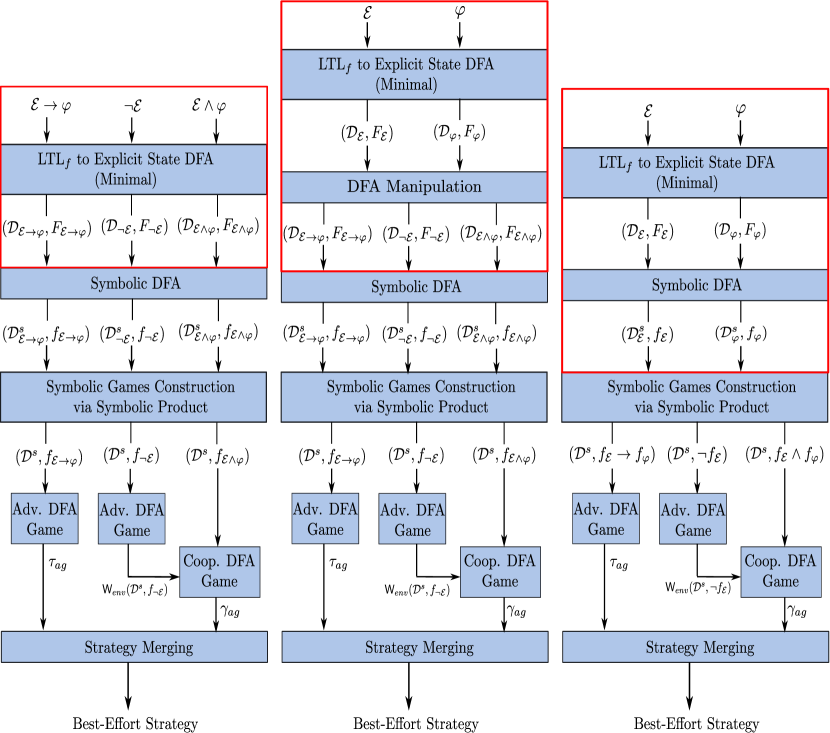
Figure 1: From left to right, (a) monolithic, (b) explicit-compositional, and (c) symbolic-compositional techniques to ltl_f best-effort synthesis. In particular, $\mathcal{D}^{s}=\mathcal{D}^{s}_{\mathcal{E}\rightarrow\varphi}\times\mathcal{D}^{s}_{\neg\mathcal{E}}\times\mathcal{D}^{s}_{\mathcal{E}\wedge\varphi}$ in (a) and (b). $\mathcal{D}^{s}=\mathcal{D}^{s}_{\mathcal{E}}\times\mathcal{D}^{s}_{\varphi}$ in (c). The specific operations of the three techniques are enclosed in red boxes.

4.1 Symbolic dfa Games 

We consider the dfa representation described in Section 3 as an explicit-state representation. Instead, we are able to represent a dfa more compactly in a symbolic way by using a logarithmic number of propositions to encode the state space. More specifically, the symbolic representation of $\mathcal{D}$ is a tuple $\mathcal{D}^{s}=(\mathcal{X},\mathcal{Y},\mathcal{Z},Z_{0},\eta)$, where $\mathcal{Z}$ is a set of state variables such that $|\mathcal{Z}|=\lceil\log|S|\rceil$, and every state $s\in S$ corresponds to an interpretation $Z\in 2^{\mathcal{Z}}$ over $\mathcal{Z}$; $Z_{0}\in 2^{\mathcal{Z}}$ is the interpretation corresponding to the initial state $s_{0}$; $\eta\colon 2^{\mathcal{X}}\times 2^{\mathcal{Y}}\times 2^{\mathcal{Z}}\rightarrow 2^{\mathcal{Z}}$ is a Boolean function such that $\eta(Z,X,Y)=Z^{\prime}$ if and only if $Z$ is the interpretation of a state $s$ and $Z^{\prime}$ is the interpretation of the state $\delta(s,X\cup Y)$. The set of goal states is represented by a Boolean function $f$ over $\mathcal{Z}$ that is satisfied exactly by the interpretations of states in $F$. In the following, we denote symbolic dfas as pairs $(\mathcal{D}^{s},f)$.

Given a symbolic dfa game $(\mathcal{D}^{s},f)$, we can compute a positional uniform winning agent strategy through a least fixpoint computation over two Boolean formulas $w$ over $\mathcal{Z}$ and $t$ over $\mathcal{Z}\cup\mathcal{Y}$, which represent the agent winning region and winning states with agent actions such that, regardless of how the environment behaves, the agent reaches the final states, respectively. Specifically, $w$ and $t$ are initialized as $w_{0}(\mathcal{Z})=f(\mathcal{Z})$ and $t_{0}(\mathcal{Z},\mathcal{Y})=f(\mathcal{Z})$, since every goal state is an agent winning state. Note that $t_{0}$ is independent of the propositions from $\mathcal{Y}$, since once the play reaches goal states, the agent can do whatever it wants. $t_{i+1}$ and $w_{i+1}$ are constructed as follows:

$$t_{i+1}(Z,Y)=t_{i}(Z,Y)\vee(\neg w_{i}(Z)\wedge\forall X.w_{i}(\eta(X,Y,Z)))$$

$$w_{i+1}(Z)=\exists Y.t_{i+1}(Z,Y)$$

The computation reaches a fixpoint when $w_{i+1}\equiv w_{i}$. To see why a fixpoint is eventually reached, note that function $w_{i+1}$ is monotonic. That is, at each step, a state $Z$ is added to the winning region $w_{i+1}$ only if it has not been already detected as a winning state, written $\neg w_{i}(Z)$ in function $t_{i+1}(Z,Y)$ above, and there exists an agent choice $Y$ such that, for every environment choice $X$, the agent moves in $w_{i}$, written $\forall X.w_{i}(\eta(X,Y,Z))$.

When the fixpoint is reached, no more states will be added, and so all agent winning states have been collected. By evaluating $Z_{0}$ on $w_{i+1}$ we can determine if there exists a winning strategy. If that is the case, $t_{i+1}$ can be used to compute a uniform positional winning strategy through the mechanism of Boolean synthesis [14]. More specifically, by passing $t_{i}$ to a Boolean synthesis procedure, setting $\mathcal{Z}$ as input variables and $\mathcal{Y}$ as output variables, we obtain a uniform positional winning strategy $\tau:2^{\mathcal{Z}}\rightarrow 2^{\mathcal{Y}}$ that can be used to induce an agent winning strategy.

Computing a uniform positional cooperatively winning strategy can be performed through an analogous least-fixpoint computation. To do this, we define again Boolean functions $\hat{w}$ over $\mathcal{Z}$ and $\hat{t}$ over $\mathcal{Z}\cup\mathcal{Y}$, now representing the agent cooperatively winning region and cooperatively winning states with agent actions such that, if the environment behaves cooperatively, the agent reaches the final states. Analogously, we initialize $\hat{w}_{0}(\mathcal{Z})=f(\mathcal{Z})$ and $\hat{t}_{0}(\mathcal{Z},\mathcal{Y})=f(\mathcal{Z})$. Then, we construct $\hat{t}_{i+1}$ and $\hat{w}_{i+1}$ as follows:

$$\hat{t}_{i+1}(Z,Y)=\hat{t}_{i}(Z,Y)\vee(\neg\hat{w}_{i}(Z)\wedge\exists X.\hat{w}_{i}(\eta(X,Y,Z)))$$

$$\hat{w}_{i+1}(Z)=\exists Y.\hat{t}_{i+1}(Z,Y);$$

Once the computation reaches the fixpoint, checking the existence and computing a uniform cooperatively winning positional strategy can be done similarly.

Sometimes, the state space of a symbolic transition system must be restricted to not reach a given set of invalid states represented as a Boolean function. To do so, we redirect all transitions from states in the set to a sink state. Formally:

Definition 6

Let $\mathcal{D}^{s}=(\mathcal{Z},\mathcal{X},\mathcal{Y},Z_{0},\eta)$ be a symbolic transition system and $g$ a Boolean formula over $\mathcal{Z}$ representing a set of states. The restriction of $\mathcal{D}^{s}$ to $g$ is a new symbolic transition system $\mathcal{D}^{\prime s}=(\mathcal{Z},\mathcal{X},\mathcal{Y},Z_{0},\eta^{\prime})$, where $\eta^{\prime}$ only agrees with $\eta$ if $Z\models g$, i.e., $\eta^{\prime}=\eta\land g$.

4.2 Monolithic Approach

The monolithic approach is a direct implementation of the best-effort synthesis approach presented in [4] (i.e., of Algorithm 0), utilizing the symbolic synthesis framework introduced in [22]. Given a best-effort synthesis problem $\mathcal{P}=(\mathcal{E},\varphi)$, we first construct the dfas following the synthesis algorithm described in Section 3, and convert them into a symbolic representation. Then, we solve suitable games on the symbolic dfas and obtain a best-effort strategy. The workflow of the monolithic approach, i.e., Algorithm 1, is shown in Figure 1(a). We elaborate on the algorithm as follows.

Algorithm 1. Given an ltl_f best-effort synthesis problem $\mathcal{P}=(\mathcal{E},\varphi)$, proceed as follows:

1. For ltl_f formulas $\mathcal{E}\rightarrow\varphi$, $\neg\mathcal{E}$ and $\mathcal{E}\wedge\varphi$ compute the corresponding minimal explicit-state dfas $\mathcal{A}_{\mathcal{E}\rightarrow\varphi}=(\mathcal{D}_{\mathcal{E}\rightarrow\varphi},F_{\mathcal{E}\rightarrow\varphi})$, $\mathcal{A}_{\neg\mathcal{E}}=(\mathcal{D}_{\neg\mathcal{E}},F_{\neg\mathcal{E}})$ and $\mathcal{A}_{\mathcal{E}\wedge\varphi}=(\mathcal{D}_{\mathcal{E}\wedge\varphi},F_{\mathcal{E}\wedge\varphi})$.

2. Convert the dfas to a symbolic representation to obtain $\mathcal{A}^{s}_{\mathcal{E}\rightarrow\varphi}=(\mathcal{D}^{s}_{\mathcal{E}\rightarrow\varphi},f_{\mathcal{E}\rightarrow\varphi})$, $\mathcal{A}^{s}_{\neg\mathcal{E}}=(\mathcal{D}^{s}_{\neg\mathcal{E}},f_{\neg\mathcal{E}})$ and $\mathcal{A}^{s}_{\mathcal{E}\wedge\varphi}=(\mathcal{D}^{s}_{\mathcal{E}\wedge\varphi},f_{\mathcal{E}\wedge\varphi})$.

3. Construct the product $\mathcal{D}^{s}=\mathcal{D}^{s}_{\mathcal{E}\rightarrow\varphi}\times\mathcal{D}^{s}_{\neg\mathcal{E}}\times\mathcal{D}^{s}_{\mathcal{E}\land\varphi}$.

4. In dfa game $(\mathcal{D}^{s},f_{\mathcal{E}\rightarrow\varphi})$, compute a uniform positional winning strategy $\tau_{{\sc ag}}$ and the agent’s winning region $\mathsf{W}_{\sc ag}(\mathcal{D}^{s},f_{\mathcal{E}\rightarrow\varphi})$.

5. In dfa game $(\mathcal{D}^{s},f_{\neg\mathcal{E}})$, compute the environment’s winning region $\mathsf{W}_{\sc env}(\mathcal{D}^{s},f_{\neg\mathcal{E}})$.

6. Compute the symbolic restriction $\mathcal{D}^{\prime s}$ of $\mathcal{D}^{s}$ to $\mathsf{W}_{\sc env}(\mathcal{D}^{s},f_{\neg\mathcal{E}})$ to restrict the state space of $\mathcal{D}^{s}$ to considering $\mathsf{W}_{\sc env}(\mathcal{D}^{s},f_{\neg\mathcal{E}})$ only.

7. In dfa game $(\mathcal{D}^{\prime s},f_{\mathcal{E}\wedge\varphi})$, compute a uniform positional cooperatively winning strategy $\gamma_{\sc ag}$.

8. Return the best-effort strategy $\sigma_{ag}$ induced by the positional strategy $\kappa_{ag}$ constructed as follows: $\kappa_{ag}(Z)=\begin{cases}\tau_{\sc ag}(Z)&\text{ if }Z\models\mathsf{W}_{\sc ag}(\mathcal{D}^{s},f_{\mathcal{E}\rightarrow\varphi})\\ \gamma_{\sc ag}(Z)&\text{ otherwise.}\end{cases}$

The main challenge in the monolithic approach comes from the ltl_f-to-dfa conversion, which can take, in the worst case, double-exponential time [11], and thus is also considered the bottleneck of ltl_f synthesis [22]. To that end, we propose an explicit-compositional approach to diminish this difficulty by decreasing the number of ltl_f-to-dfa conversions.

4.3 Explicit-Compositional Approach

As described in Section 4.2, the monolithic approach to a best-effort synthesis problem $\mathcal{P}=(\mathcal{E},\varphi)$ involves three rounds of ltl_f-to-dfa conversions corresponding to ltl_f formulas $\mathcal{E}\rightarrow\varphi$, $\neg\mathcal{E}$ and $\mathcal{E}\wedge\varphi$. However, observe that dfas $\mathcal{A}_{\mathcal{E}\rightarrow\varphi}$, $\mathcal{A}_{\neg\mathcal{E}}$ and $\mathcal{A}_{\mathcal{E}\wedge\varphi}$ can, in fact, be constructed by manipulating the two dfas $\mathcal{A}_{\mathcal{E}}$ and $\mathcal{A}_{\varphi}$ of ltl_f formulas $\mathcal{E}$ and $\varphi$, respectively. Specifically, given the explicit-state dfas $\mathcal{A}_{\varphi}$ and $\mathcal{A}_{\mathcal{E}}$, we obtain $\mathcal{A}_{\mathcal{E}\rightarrow\varphi}$, $\mathcal{A}_{\neg\mathcal{E}}$ and $\mathcal{A}_{\mathcal{E}\wedge\varphi}$ as follows:

• $\mathcal{A}_{\mathcal{E}\rightarrow\varphi}=\mathsf{Comp}(\mathsf{Inter}(\mathcal{A}_{\mathcal{E}},\mathsf{Comp}(\mathcal{A}_{\varphi}))$;

• $\mathcal{A}_{\neg\mathcal{E}}=\mathsf{Comp}(\mathcal{A}_{\mathcal{E}})$;

• $\mathcal{A}_{\mathcal{E}\wedge\varphi}=\mathsf{Inter}(\mathcal{A}_{\mathcal{E}},\mathcal{A}_{\varphi})$;

where $\mathsf{Comp}$ and $\mathsf{Inter}$ denote complement and intersection on explicit-state dfas, respectively. Note that transforming ltl_f formulas into dfas takes double-exponential time in the size of the formula, while the complement and intersection of dfas take polynomial time in the size of the dfa.

The workflow of the explicit-compositional approach, i.e., Algorithm 2, is shown in Figure 1(b). As the monolithic approach, we first translate the formulas $\mathcal{E}$ and $\varphi$ into minimal explicit-state dfas $\mathcal{A}_{\mathcal{E}}$ and $\mathcal{A}_{\varphi}$, respectively. Then, dfas $\mathcal{A}_{\mathcal{E}\rightarrow\varphi}$, $\mathcal{A}_{\neg\mathcal{E}}$ and $\mathcal{A}_{\mathcal{E}\wedge\varphi}$ are constructed by manipulating $\mathcal{A}_{\mathcal{E}}$ and $\mathcal{A}_{\varphi}$ through complement and intersection. Indeed, the constructed explicit-state dfas are also minimized. The remaining steps of computing suitable dfa games are the same as in the monolithic approach.

4.4 Symbolic-Compositional Approach

The monolithic and explicit-compositional approaches are based on playing three games over the symbolic product of transition systems $\mathcal{D}_{\mathcal{E}\rightarrow\varphi}$, $\mathcal{D}_{\neg\mathcal{E}}$, and $\mathcal{D}_{\mathcal{E}\land\varphi}$. We observe that given dfas $\mathcal{A}_{\mathcal{E}}=(\mathcal{D}_{\mathcal{E}},F_{\mathcal{E}})$ and $\mathcal{A}_{\varphi}=(\mathcal{D}_{\varphi},F_{\varphi})$ recognizing $\mathcal{E}$ and $\varphi$, respectively, the dfa recognizing any Boolean combination of $\mathcal{E}$ and $\varphi$ can be constructed by taking the product of $\mathcal{D}_{\mathcal{E}}$ and $\mathcal{D}_{\varphi}$ and properly defining the set of final states over the resulting transition system.

Lemma 1

Let $\mathcal{A}_{\psi_{1}}=(\mathcal{D}_{\psi_{1}},F_{\psi_{1}})$ and $\mathcal{A}_{\psi_{2}}=(\mathcal{D}_{\psi_{2}},F_{\psi_{2}})$ be the automata recognizing ltl_f formulas $\psi_{1}$ and $\psi_{2}$, respectively, and $\psi=\psi_{1}\ op\ \psi_{2}$ denoting an arbitrary Boolean combination of $\psi_{1}$ and $\psi_{2}$, i.e., $op\in\{\land,\lor,\rightarrow,\leftrightarrow\}$. The dfa $\hat{\mathcal{A}_{\psi}}=(\hat{\mathcal{D}_{\psi}},\hat{F}_{\psi})$ with $\hat{\mathcal{D}_{\psi}}=\mathcal{D}_{\psi_{1}}\times\mathcal{D}_{\psi_{2}}$ and $\hat{F}_{\psi}=\{(s_{\psi_{1}},s_{\psi_{2}})\ |\ s_{\psi_{1}}\in F_{\psi_{1}}\ op\ s_{\psi_{2}}\in F_{\psi_{2}}\}$ recognizes $\psi$.

Proof

($\rightarrow$) Assume $\pi\models\psi$. We will prove that $\pi\in\mathcal{L}(\hat{\mathcal{A}}_{\varphi})$. To see this, observe that $\pi\models\psi$ implies $\pi\models\psi_{1}\ op\ \pi\models\psi_{2}$. It follows by [11] that $\pi\in\mathcal{L}(\mathcal{A}_{\psi_{1}})\ op\ \pi\in\mathcal{L}(\mathcal{A}_{\psi_{2}})$, meaning that running $\pi$ in $\mathcal{D}_{\psi_{1}}$ and $\mathcal{D}_{\psi_{2}}$ yields the sequences of states $(s_{0}^{\psi_{1}},\ldots,s_{n}^{\psi_{1}})$ and $(s_{0}^{\psi_{2}},\ldots,s_{n}^{\psi_{2}})$ such that $s_{n}^{\psi_{1}}\in F_{\psi_{1}}\ op\ s_{n}^{\psi_{2}}\in F_{\psi_{2}}$. Since $\hat{\mathcal{D}}_{\psi}$ is obtained through synchronous product of $\mathcal{D}_{\psi_{1}}$ and $\mathcal{D}_{\psi_{2}}$, running $\pi$ in $\hat{\mathcal{A}}_{\psi}$ yields the sequence of states $((s_{0}^{\psi_{1}},s_{0}^{\psi_{2}}),\ldots,(s_{n}^{\psi_{1}},s_{n}^{\psi_{2}}))$, such that $(s_{n}^{\psi_{1}},s_{n}^{\psi_{2}})\in\hat{F}_{\psi}$. Hence, we have that $\pi\in\mathcal{L}(\hat{\mathcal{A}}_{\psi})$.
($\leftarrow$) Assume $\pi\in\mathcal{L}(\hat{\mathcal{A}}_{\varphi})$. We prove that $\pi\models\psi$. To see this, observe that $\pi\in\mathcal{L}(\hat{\mathcal{A}}_{\varphi})$ means that the run $\rho=(s_{0}^{\psi_{1}},s_{0}^{\psi_{2}})\ldots(s_{n}^{\psi_{1}},s_{n}^{\psi_{2}})$ induced by $\pi$ on $\hat{\mathcal{D}}_{\psi}$ is such that $(s_{n}^{\psi_{1}},s_{n}^{\psi_{2}})\in\hat{F}_{\psi}$. This means, by construction of $\hat{F}_{\psi}$, that $(s_{n}^{\psi_{1}},s_{n}^{\psi_{2}})\text{ s.t. }s_{n}^{\psi_{1}}\in F_{\psi_{1}}\ op\ s_{n}^{\psi_{2}}\in F_{\psi_{2}}$. Since $\hat{\mathcal{D}}_{\psi}$ is obtained through synchronous product of $\mathcal{D}_{\psi_{1}}$ and $\mathcal{D}_{\psi_{2}}$, it follows that $\pi\in\mathcal{L}(\mathcal{A}_{\psi_{1}})\ op\ \pi\in\mathcal{L}(\mathcal{A}_{\psi_{2}})$. By [11] we have that $\pi\models\psi_{1}\ op\ \pi\models\psi_{2}$, and hence $\pi\models\psi$.

Notably, Lemma 1 tells that the dfas $\mathcal{A}_{\mathcal{E}\rightarrow\varphi}$, $\mathcal{A}_{\neg\mathcal{E}}$, and $\mathcal{A}_{\mathcal{E}\land\varphi}$ can be constructed from the same transition system by defining proper sets of final states. Specifically, given the dfas $\mathcal{A}_{\mathcal{E}}=(\mathcal{D}_{\mathcal{E}},F_{\mathcal{E}})$ and $\mathcal{A}_{\varphi}=(\mathcal{D}_{\varphi},F_{\varphi})$ recognizing $\mathcal{E}$ and $\varphi$, respectively, the dfas recognizing $\mathcal{E}\rightarrow\varphi$, $\neg\mathcal{E}$, and $\mathcal{E}\land\varphi$ can be constructed as $\mathcal{A}_{\mathcal{E}\rightarrow\varphi}=(\mathcal{D},F_{\mathcal{E}\rightarrow\varphi})$, $\mathcal{A}_{\neg\mathcal{E}}=(\mathcal{D},F_{\neg\mathcal{E}})$, and $\mathcal{A}_{\mathcal{E}\land\varphi}=(\mathcal{D},F_{\mathcal{E}\land\varphi})$, respectively, where $\mathcal{D}=\mathcal{D}_{\mathcal{E}}\times\mathcal{D}_{\varphi}$ and:

• $F_{\mathcal{E}\rightarrow\varphi}=\{(s_{\mathcal{E}},s_{\varphi})\mid s_{\mathcal{E}}\in F_{\mathcal{E}}\rightarrow s_{\varphi}\in F_{\varphi}\}$.

• $F_{\neg\mathcal{E}}=\{(s_{\mathcal{E}},s_{\varphi})\mid s_{\mathcal{E}}\not\in F_{\mathcal{E}}\}$.

• $F_{\mathcal{E}\land\varphi}=\{(s_{\mathcal{E}},s_{\varphi})\mid s_{\mathcal{E}}\in F_{\mathcal{E}}\land s_{\varphi}\in F_{\varphi}\}$.

The symbolic-compositional approach precisely bases on this observation. As shown in Figure 1(c), we first transform the ltl_f formulas $\mathcal{E}$ and $\varphi$ into minimal explicit-state dfas $\mathcal{A}_{\mathcal{E}}$ and $\mathcal{A}_{\varphi}$, respectively, and then construct the symbolic representations $\mathcal{A}^{s}_{\mathcal{E}}$ and $\mathcal{A}^{s}_{\varphi}$ of them. Subsequently, we construct the symbolic product $\mathcal{D}^{s}=\mathcal{D}^{s}_{\mathcal{E}}\times\mathcal{D}^{s}_{\varphi}$, once and for all, and get the three dfa games by defining the final states (which are Boolean functions) from $f_{\mathcal{E}}$ and $f_{\varphi}$ as follows:

• $f_{\mathcal{E}\rightarrow\varphi}=f_{\mathcal{E}}\rightarrow f_{\varphi}$.

• $f_{\neg\mathcal{E}}=\neg f_{\mathcal{E}}$.

• $f_{\mathcal{E}\wedge\varphi}=f_{\mathcal{E}}\wedge f_{\varphi}$.

From now on, the remaining steps are the same as in the monolithic and explicit-compositional approaches.

Algorithm 3. Given a best-effort synthesis problem $\mathcal{P}=(\mathcal{E},\varphi)$, proceed as follows:

1. Compute the minimal explicit-state dfas $\mathcal{A}_{\mathcal{E}}=(\mathcal{D}_{\mathcal{E}},F_{\mathcal{E}})$ and $\mathcal{A}_{\varphi}=(\mathcal{D}_{\varphi},F_{\varphi})$.

2. Convert the dfas to a symbolic representation to obtain $\mathcal{A}^{s}_{\mathcal{E}}=(\mathcal{D}^{s}_{\mathcal{E}},f_{\mathcal{E}})$ and $\mathcal{A}^{s}_{\varphi}=(\mathcal{D}^{s}_{\varphi},f_{\varphi})$.

3. Construct the symbolic product $\mathcal{D}^{s}=\mathcal{D}^{s}_{\mathcal{E}}\times\mathcal{D}^{s}_{\varphi}$.

4. In dfa game $\mathcal{G}^{s}_{\mathcal{E}\rightarrow\varphi}=(\mathcal{D}^{s},f_{\mathcal{E}}\rightarrow f_{\varphi})$ compute a positional uniform winning strategy $\tau_{ag}$ and the agent winning region $\mathsf{W}_{\sc ag}(\mathcal{D}^{s},f_{\mathcal{E}}\rightarrow f_{\varphi})$.

5. In the dfa game $(\mathcal{D}^{s},\neg f_{\mathcal{E}})$ compute the environment’s winning region $\mathsf{W}_{\sc env}(\mathcal{D}^{s},\neg f_{\mathcal{E}})$.

6. Compute the symbolic restriction $\mathcal{D}^{\prime s}$ of $\mathcal{D}^{s}$ to $\mathsf{W}_{\sc env}(\mathcal{D}^{s},f_{\neg\mathcal{E}})$ so as to restrict the state space of $\mathcal{D}^{s}$ to considering $\mathsf{W}_{\sc env}(\mathcal{D}^{s},f_{\neg\mathcal{E}})$ only.

7. In the dfa game $(\mathcal{D}^{\prime s},f_{\mathcal{E}}\wedge f_{\varphi})$ find a positional cooperatively winning strategy $\gamma_{ag}$.

8. Return the best-effort strategy $\sigma_{ag}$ induced by the positional strategy $\kappa_{ag}$ constructed as follows: $\kappa_{ag}(Z)=\begin{cases}\tau_{\sc ag}(Z)&\text{ if }Z\models\mathsf{W}_{\sc ag}(\mathcal{D}^{s},f_{\mathcal{E}\rightarrow\varphi})\\ \gamma_{\sc ag}(Z)&\text{ otherwise.}\end{cases}$

5 Empirical Evaluations

In this section, we first describe how we implemented our symbolic ltl_f best-effort synthesis approaches described in Section 4. Then, by empirical evaluation, we show that Algorithm 3, i.e., the symbolic-compositional approach, shows an overall best-performance. In particular, we show that performing best-effort synthesis only brings a minimal overhead with respect to standard synthesis and may even show better performance on certain instances.

5.1 Implementation

We implemented the three symbolic approaches to ltl_f best-effort synthesis described in Section 4 in a tool called BeSyft, by extending the symbolic synthesis framework [22, 20] integrated in state-of-the-art synthesis tools [6, 9]. In particular, we based on Lydia , the overall best performing ltl_f-to-dfa conversion tool, to construct the minimal explicit-state dfas of ltl_f formulas. Moreover, BeSyft borrows the rich APIs from Lydia to perform relevant explicit-state dfa manipulations required by both Algorithm 1, i.e., the monolithic approach (c.f., Subsection 4.2), and Algorithm 2, i.e., the explicit-compositional approach (c.f., Subsection 4.3), such as complement, intersection, minimization. As in [22, 20], the symbolic dfa games are represented in Binary Decision Diagrams (BDDs) [7], utilizing CUDD-3.0.0 [19] as the BDD library. Thereby, BeSyft constructs and solves symbolic dfa games using Boolean operations provided by CUDD-3.0.0, such as negation, conjunction, and quantification. The uniform positional winning strategy $\tau_{\sc ag}$ and the uniform positional cooperatively winning strategy $\gamma_{\sc ag}$ are computed utilizing Boolean synthesis [14]. The positional best-effort strategy is obtained by applying suitable Boolean operations on $\tau_{\sc ag}$ and $\gamma_{\sc ag}$. As a result, we have three derivations of BeSyft, namely BeSyft-Alg-1, BeSyft-Alg-2, and BeSyft-Alg-3, corresponding to the monolithic, explicit-compositional, and symbolic-compositional approach, respectively.

5.2 Experiment Methodology

Experiment Setup.

All experiments were run on a laptop with an operating system 64-bit Ubuntu 20.04, 3.6 GHz CPU, and 12 GB of memory. Time out was set to 1000 seconds.

Benchmarks.

We devised a counter-game benchmark, based on the one proposed in [21]. More specifically, there is an $n$-bit binary counter and, at each round, the environment chooses whether to issue an increment request for the counter or not. The agent can choose to grant the request or ignore it and its goal is to get the counter to have all bits set to $1$. The increment requests only come from the environment, and occur in accordance with the environment specification. The size of the minimal dfa of a counter-game specification grows exponentially as $n$ increases.

In the experiments, environment specifications ensure that the environment eventually issues a minimum number $K$ of increment requests in sequence, which can be represented as ltl_f formulas $\mathcal{E}_{K}=\Diamond(add\wedge\raisebox{-1.1625pt}{\LARGE$\bullet$}(add)\ldots\wedge\raisebox{-1.1625pt}{\LARGE$\bullet$}(\ldots(\raisebox{-1.1625pt}{\LARGE$\bullet$}(add))\ldots))$, where $K$ is the number of conjuncts. Counter-game instances may be realizable depending on the parameter $K$ and the number of bits $n$. In the case of a realizable instance, a strategy for the agent to enforce the goal is to grant all increment requests coming from the environment. Else, the agent can achieve the goal only if the environment behaves cooperatively, such as issuing more increment requests than that specified in the environment specification. That is, the agent needs a best-effort strategy. In our experiments, we considered counter-game instances with at most $n=10$ bits and $K=10$ sequential increment requests. As a result, our benchmarks consist of a total of $100$ instances.

5.3 Experimental Results and Analysis.

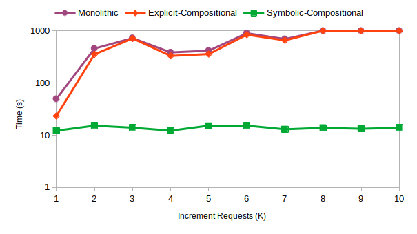
Figure 2: Comparison (in log scale) of BeSyft implementations on counter game instances with $n=8$ and $1\leq K\leq 10$.

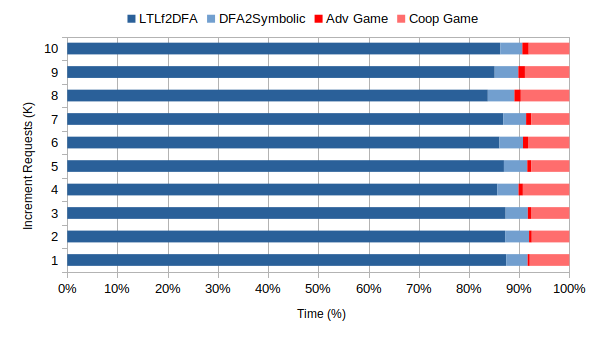
Figure 3: Relative time cost of BeSyft-Alg-3 major operations on counter game instances with $n=8$ and $1\leq K\leq 10$.

In our experiments, all BeSyft implementations are only able to solve counter-game instances with up to $n=8$ bits. Figure 2 shows the comparison (in log scale) of the three symbolic implementations of best-effort synthesis on counter-game instances with $n=8$ and $1\leq K\leq 10$. First, we observe that BeSyft-Alg-1 (monolithic) and BeSyft-Alg-2 (explicit-compositional) reach timeout when $K\geq 8$, whereas BeSyft-Alg-3 (symbolic-compositional) is able to solve all $8$-bit counter-game instances. We can also see that BeSyft-Alg-1 performs worse than the other two derivations since it requires three rounds of ltl_f-to-dfa conversions, which in the worst case, can lead to a double-exponential blowup. Finally, we note that BeSyft-Alg-3, which implements the symbolic-compositional approach, achieves orders of magnitude better performance than the other two implementations, although it does not fully exploit the power of dfa minimization. Nevertheless, it is not the case that automata minimization always leads to improvement. Instead, there is a tread-off of performing automata minimization. As shown in Figure 2, BeSyft-Alg-3, performs better than BeSyft-Alg-2, though the former does not minimize the game arena after the symbolic product, and the latter minimizes the game arena as much as possible.

On a closer inspection, we evaluated the time cost of each major operation of BeSyft-Alg-3, and present the results on counter-game instances with $n=8$ and $1\leq K\leq 10$ in Figure 3. First, the results show that ltl_f-to-dfa conversion is the bottleneck of ltl_f best-effort synthesis, the cost of which dominates the total running time. Furthermore, we can see that the total time cost of solving the cooperative dfa game counts for less than $10\%$ of the total time cost. As a result, we conclude that performing best-effort synthesis only brings a minimal overhead with respect to standard reactive synthesis, which consists of constructing the dfa of the input ltl_f formula and solving its corresponding adversarial game. Also, we observe that solving the cooperative game takes longer than solving the adversarial game. Indeed, this is because the fixpoint computation in the cooperative game often requires more iterations than that in the adversarial game.

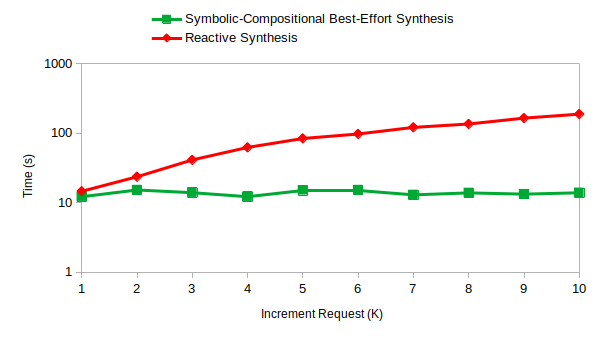
Figure 4: Comparison (in log scale) of BeSyft-Alg-3 and implementations of symbolic ltl_f reactive synthesis on counter-game instances with $n=8$ and $1\leq K\leq 10$.

Finally, we also compared the time cost of symbolic-compositional best-effort synthesis with that of standard reactive synthesis on counter-game instances. More specifically, we considered a symbolic implementation of reactive synthesis that computes an agent strategy that enforces the ltl_f formula $\mathcal{E}\rightarrow\varphi$ [10, 22], which can be used to find an agent strategy enforcing $\varphi$ under $\mathcal{E}$, if it exists [3]. Interestingly, Figure 4 shows that for certain counter-game instances, symbolic-compositional best-effort synthesis takes even less time than standard reactive synthesis. It should be noted that symbolic-compositional best-effort synthesis performs ltl_f-to-dfa conversions of ltl_f formulas $\varphi$ and $\mathcal{E}$ separately and combines them to obtain the final game arena without having automata minimization, whereas reactive synthesis performs the ltl_f-to-dfa conversion of formula $\mathcal{E}\rightarrow\varphi$ and minimizes its corresponding dfa. These results confirm the practical feasibility of best-effort synthesis and that automata minimization does not always guarantee performance improvement.

6 Conclusion 

We presented three different symbolic ltl_f best-effort synthesis approaches: monolithic, explicit-compositional, and symbolic-compositional. Empirical evaluations proved the outperformance of the symbolic-compositional approach. An interesting observation is that, although previous studies suggest taking the maximal advantage of automata minimization [20, 21], in the case of ltl_f best-effort synthesis, there can be a trade-off in doing so. Another significant finding is that the best-performing ltl_f best-effort synthesis approach only brings a minimal overhead compared to standard synthesis. Given this nice computational result, a natural future direction would be looking into ltl_f best-effort synthesis with multiple environment assumptions [1].

References

- [1] Aminof, B., De Giacomo, G., Lomuscio, A., Murano, A., Rubin, S.: Synthesizing best-effort strategies under multiple environment specifications. In: KR. pp. 42–51 (2021)
- [2] Aminof, B., De Giacomo, G., Murano, A., Rubin, S.: Planning and synthesis under assumptions. arXiv (2018)
- [3] Aminof, B., De Giacomo, G., Murano, A., Rubin, S.: Planning under LTL environment specifications. In: ICAPS. pp. 31–39 (2019)
- [4] Aminof, B., De Giacomo, G., Rubin, S.: Best-effort synthesis: Doing your best is not harder than giving up. In: IJCAI. pp. 1766–1772 (2021)
- [5] Baier, C., Katoen, J.P.: Principles of Model Checking. MIT Press (2008)
- [6] Bansal, S., Li, Y., Tabajara, L.M., Vardi, M.Y.: Hybrid compositional reasoning for reactive synthesis from finite-horizon specifications. In: AAAI. pp. 9766–9774 (2020)
- [7] Bryant, R.E.: Symbolic boolean manipulation with ordered binary-decision diagrams. ACM Comput. Surv. 24(3), 293–318 (1992)
- [8] Cimatti, A., Pistore, M., Roveri, M., Traverso, P.: Weak, strong, and strong cyclic planning via symbolic model checking. AIJ 1–2(147), 35–84 (2003)
- [9] De Giacomo, G., Favorito, M.: Compositional approach to translate LTLf/LDLf into deterministic finite automata. In: ICAPS. pp. 122–130 (2021)
- [10] De Giacomo, G., Favorito, M.: Lydia: A tool for compositional LTLf /LDLf synthesis. In: ICAPS. pp. 122–130 (2021)
- [11] De Giacomo, G., Vardi, M.Y.: Linear temporal logic and linear dynamic logic on finite traces. In: IJCAI. pp. 854–860 (2013)
- [12] De Giacomo, G., Vardi, M.Y.: Synthesis for LTL and LDL on Finite Traces. In: IJCAI. pp. 1558–1564 (2015)
- [13] Finkbeiner, B.: Synthesis of reactive systems. Dependable Software Systems Eng. 45, 72–98 (2016)
- [14] Fried, D., Tabajara, L.M., Vardi, M.Y.: BDD-based Boolean functional synthesis. In: CAV. pp. 402–421 (2016)
- [15] Ghallab, M., Nau, D.S., Traverso, P.: Automated planning - theory and practice. Elsevier (2004)
- [16] Henriksen, J.G., Jensen, J.L., Jørgensen, M.E., Klarlund, N., Paige, R., Rauhe, T., Sandholm, A.: Mona: Monadic second-order logic in practice. In: TACAS. pp. 89–110 (1995)
- [17] Pnueli, A., Rosner, R.: On the synthesis of a reactive module. In: POPL. p. 179–190 (1989)
- [18] Pnueli, A.: The temporal logic of programs. In: FOCS. pp. 46–57 (1977)
- [19] Somenzi, F.: CUDD: CU Decision Diagram Package 3.0.0. Universiy of Colorado at Boulder (2016)
- [20] Tabajara, L.M., Vardi, M.Y.: Partitioning techniques in LTLf synthesis. In: IJCAI. pp. 5599–5606 (2019)
- [21] Zhu, S., De Giacomo, G., Pu, G., Vardi, M.Y.: LTLf synthesis with fairness and stability assumptions. In: AAAI. pp. 3088–3095 (2020)
- [22] Zhu, S., Tabajara, L.M., Li, J., Pu, G., Vardi, M.Y.: Symbolic LTLf synthesis. In: IJCAI. pp. 1362–1369 (2017)