Domain Walls and Vector Solitons in the Coupled Nonlinear Schrödinger Equation
Abstract
We outline a program to classify domain walls (DWs) and vector solitons in the 1D two-component coupled nonlinear Schrödinger (CNLS) equation without restricting the signs or magnitudes of any coefficients. The CNLS equation is reduced first to a complex ordinary differential equation (ODE), and then to a real ODE after imposing a restriction. In the real ODE, we identify four possible equilibria including ZZ, ZN, NZ, and NN, with Z (N) denoting a zero (nonzero) value in a component, and analyze their spatial stability. We identify two types of DWs including asymmetric DWs between ZZ and NN and symmetric DWs between ZN and NZ. We identify three codimension-1 mechanisms for generating vector solitons in the real ODE including heteroclinic cycles, local bifurcations, and exact solutions. Heteroclinic cycles are formed by assembling two DWs back-to-back and generate extended bright-bright (BB), dark-dark (DD), and dark-bright (DB) solitons. Local bifurcations include the Turing (Hamiltonian-Hopf) bifurcation that generates Turing solitons with oscillatory tails and the pitchfork bifurcation that generates DB, bright-antidark, DD, and dark-antidark solitons with monotonic tails. Exact solutions include scalar bright and dark solitons with vector amplitudes. Any codimension-1 real vector soliton can be numerically continued into a codimension-0 family. Complex vector solitons have two more parameters: a dark or antidark component can be numerically continued in the wavenumber, while a bright component can be multiplied by a constant phase factor. We introduce a numerical continuation method to find real and complex vector solitons and show that DWs and DB solitons in the immiscible regime can be related by varying bifurcation parameters. We show that collisions between two DB solitons with a nonzero phase difference in their bright components typically feature a mass exchange that changes the frequencies and phases of the two bright components and the two soliton velocities.
1 Introduction
The nonlinear Schrödinger (NLS) equation is well known to provide a universal description of the envelope dynamics of quasi-monochromatic plane waves in weakly nonlinear dispersive systems [1, 2]. The most remarkable feature of the NLS equation is complete integrability, which enables analytical solutions to be found via the inverse scattering transform for arbitrary initial conditions [3, 4]. As a natural progression, coupled NLS (CNLS) equations arise when multiple waves interact nonlinearly, as already noted in early studies [5, 6]. Subsequently, such equations find prominent applications in diverse settings including birefringent optical fibers [7], photorefractive materials [8, 9], topological photonics [10], water waves [11, 12], coupled sine-Gordon equations [13], and many others. Much recent interest in CNLS equations relates to Bose-Einstein condensates (BECs), where an -component CNLS equation, often called the Gross-Pitaevskii equation (GPE), describes BECs with bosonic components in the mean field limit [14, 15]. Here we consider a 1D two-component CNLS equation with general coefficients, which is a homogeneous GPE without trapping potential in certain parameter regimes:
| (1) | |||
where and are complex fields, and and are real constants. If , then Eq. (1) is completely integrable when , , [16, 17, 18]. If in addition , Eq. (1) becomes the celebrated Manakov system [5], which is focusing when and defocusing when .
A fundamental feature of nonlinear wave equations is the possible balance of dispersion and nonlinearity to produce robust localized traveling waves embedded in a single plane wave, which are known as solitons (solitary waves) [19, 20, 21]. For the scalar NLS equation, it is well known that focusing NLS admits bright solitons, while defocusing NLS admits dark (grey) solitons [2, 21]. There is also a thorough catalogue of vector solitons and their interactions in the integrable CNLS equation, including bright-bright (BB) solitons in the focusing Manakov system [5, 22, 23, 24] and dark-bright (DB) and dark-dark (DD) solitons in the defocusing Manakov system [25, 26, 27, 28, 29, 30, 31]. Such solutions have been generalized to the symmetric CNLS equation () in both focusing [32, 33, 34] and defocusing [35, 29] cases.
In the binary BEC setting, there is much interest in DB and DD solitons in the defocusing regime of Eq. (1) [36]. Most of these studies assume , namely equal masses for the two species, with free parameters . The oscillation and collision dynamics of DB solitons in a harmonic trap are revealed in a pioneering theoretical study [37]. The formation of DD solitons is also predicted from the interaction of dark solitons in different components in the miscible regime [38]. Subsequently, families of vector solitons are produced that include not only DB and DD solitons, but also bright-antidark (BAD) and dark-antidark (DAD) solitons, where antidark means a hump rather than a dip in a nonzero background [39]. DB solitons are first realized experimentally using a phase imprinting method [40]. Subsequently, an alternative method is proposed to generate trains of DB solitons from the counterflow of two superfluids [41], which motivates further theoretical and experimental studies on the interaction dynamics of DB solitons [42, 43, 44]. DB solitons are also found in Eq. (1) with unequal masses (dispersion coefficients) in both [45] and [46, 47] cases. In both cases, it is found that DB solitons with a one-hump bright component could coexist with those whose bright component has two or more humps.
In addition to various solitons reviewed above, some nonlinear partial differential equations (PDEs) like Eq. (1) also admit localized traveling waves connecting two different plane waves, which are known by various names including domain walls (DWs), fronts, and kinks. Such solutions play a central role in dissipative systems in various settings [48, 49, 50, 51]. They are also found in some scalar 1D conservative (dispersive) systems, possibly with dissipative (diffusive) perturbations, such as the modified Korteweg-de Vries-Burgers equation [52] and the NLS equations with stimulated Raman scattering [53]. In general, the time evolution of an initial step between two plane waves in a dispersive system is the core topic in the field of dispersive hydrodynamics, which reformulates the original PDE as a system of hyperbolic conservation laws [54]. In this framework, dispersive shock waves arise when the flux is convex, while rarefaction waves and DWs (kinks) arise when the flux is non-convex [55].
In two-component 1D conservative systems, such as Eq. (1) in the defocusing regime, DWs can form between the two components [51]. In the optics setting, such DWs in the symmetric CNLS equation, known as polarization domain walls (PDWs), are indeed predicted theoretically [56, 57, 58, 59]. While there are early experimental indications of PDWs [60, 61], the first direct observation of PDWs is only made recently in optical fibres with potential applications to optical data transmission [62]. Applications of optical bistability to the design of photonic memory devices are also explored in recent work [63, 64]. In the binary BEC setting, DWs are found in the symmetric CNLS equation with a trapping potential [39] and possibly also linear interconversion terms [65]. More generally, in the asymmetric CNLS equation, i.e., Eq. (1) with and free parameters , DWs are found when the immiscibility condition holds [66, 67, 68].
The above studies typically make two assumptions on the coefficients of Eq. (1) that are relevant in the optics and/or BEC setting, the first being , or more often , and the second being , or equivalently by rescaling variables. However, even if both are assumed, certain parameter regimes beyond the traditional dichotomy between the focusing and the defocusing regimes are rarely explored. Moreover, in the general problem of two interacting quasi-monochromatic plane waves, often applies, but and are both very common. As we shall see, for DWs and vector solitons, there is a simple relation between solutions found at and those found at . Thus, in this paper, we outline a program to classify DWs and vector solitons in Eq. (1) without restricting the signs or magnitudes of any coefficients.
This paper is organized as follows. In Section 2, we reduce Eq. (1) first to an ordinary differential equation (ODE) with complex coefficients, and then to an ODE with real coefficients after imposing a restriction. In the real ODE, we identify all possible equilibria and analyze their spatial stability. In Section 3, we identify all possible DWs between two equilibria and construct their parameter space. In Section 4, we identify three codimension-1 mechanisms for generating vector solitons in the real ODE including heteroclinic cycles, local bifurcations, and exact solutions. Heteroclinic cycles are formed by assembling two DWs back-to-back. All possible local bifurcations on the four equilibria are identified. Exact solutions include scalar bright and dark solitons with vector amplitudes. We classify these codimension-1 real vector solitons by their types and parities and discuss numerical continuation of any such solution into a codimension-0 family. We construct the parameter space of complex vector solitons depending on whether the two components are bright, dark, or antidark. In Section 5, we introduce a numerical continuation method to find real and complex vector solitons and apply this method to DWs and DB solitons in the immiscible regime. In Section 6, we study collisions between two DB solitons with a nonzero phase difference in their bright components. The paper concludes in Section 7.
2 Equilibria and their spatial stability
To find DWs connecting two arbitrary plane waves and vector solitons embedded in an arbitrary plane wave, we apply the following traveling wave reduction to Eq. (1): , , where are complex envelopes dependent only on the comoving variable , with the group velocity of the envelope, and and are the respective wavenumbers and frequencies. This reduces Eq. (1) to a coupled system of ODEs in :
| (2) | ||||
In this framework, a plane wave in Eq. (1) corresponds to an equilibrium in Eq. (2), namely a -independent solution to Eq. (2). Thus, a DW connecting two plane waves in Eq. (1) corresponds to a heteroclinic orbit between two equilibria in Eq. (2), and a vector soliton embedded in a plane wave in Eq. (1) corresponds to a homoclinic orbit to an equilibrium in Eq. (2). We note that prior work, e.g. Ref. [45], often sets since traveling waves can be obtained from stationary waves using the Galilean transformation, but we shall keep as a free parameter in this paper to emphasize that both DWs and vector solitons can have nonzero velocities; see e.g. Ref. [69].
Once DWs and vector solitons are found in Eq. (2), their temporal stability in Eq. (1) can be determined using established methods. The temporal stability of plane waves, namely modulational instability, in Eq. (1) is already addressed in an early study [70]. However, a localized structure can be temporally unstable even if its plane wave background(s) are temporally stable [71]. In this section, we shall focus on the general existence of DWs and vector solitons, and we shall keep such solutions even if they are temporally unstable. Although temporally unstable solutions are less interesting than temporally stable ones, they can still be important for understanding the nonlinear dynamics of modulational instability and other complex spatiotemporal dynamics. Besides, our overall strategy is to first find solutions in a (typically codimension-1) subset of the parameter space that is analytically tractable, and then use these solutions as starting points for numerical continuations into the full parameter space. Even if a starting point is temporally unstable, it should not be discarded since the numerical continuation could yield temporally stable solutions.
2.1 The complex ODE
The key property of Eq. (2) that enables the existence of homoclinic orbits is its reversibility under the action
| (3) |
where and denotes complex conjugation. This reversibility represents a reflection symmetry in the phase space of Eq. (2) and implies the generic existence of homoclinic orbits to an equilibrium [72]. We observe that if is reversible under , then is reversible under . Thus, we only need to find homoclinic orbits reversible under , and the full solution family follows from multiplying each component by a constant phase factor. We need to obtain all possible solutions, but we only need to obtain all possible reversibility symmetries in Eq. (3).
The equilibria of Eq. (2), denoted as , can be classified into four types, denoted respectively as , , , and , with corresponding to zero (nonzero) values. There is a circle of equivalent equilibria in the complex plane for each nonzero component, so represents a single equilibrium, or represents a circle of equivalent equilibria, and represents a torus of equivalent equilibria. Thus, under suitable conditions, we expect a discrete, not continuous, family of homoclinic orbits connecting the two equilibria and that are equivalent under the reversibility .
Our theoretical framework of seeking solutions to a nonlinear PDE via its reduction to a spatial ODE, known as spatial dynamics [72, 50], provides a systematic method to find localized structures. For generic parameter choices, neither the original PDE in Eq. (1) nor the spatial ODE in Eq. (2) is integrable, and this non-integrable regime is the focus of this paper. However, even in the integrable regime of Eq. (1), namely the scalar NLS equation or the Manakov system, spatial dynamics can still be used to reproduce scalar or vector solitons originally derived using integrable systems theory.
2.2 The real ODE
Although Eq. (2) provides the general setting for finding DWs and vector solitons, it is rather technical to work with since it is a second-order ODE with two complex fields, or equivalently an 8D real dynamical system. Therefore, we will first seek DWs and vector solitons in Eq. (2) with the restriction
| (4) |
and then extend these solutions to Eq. (2) without this restriction. After applying Eq. (4), Eq. (2) becomes the following ODE with real coefficients:
| (5) | ||||
where
| (6) |
Thus, Eq. (6) implies that Eq. (5) is invariant under the parameter transformation , which is an ODE version of the Galilean transformation. The four types of equilibria of Eq. (5) are respectively given by
| (7) | ||||
The restriction of Eq. (5) to yields the real ODE
| (8) | ||||
The equilibria of Eq. (8) are given by Eq. (7) but restricted to the real axis, so the component can have either sign. The possible reversibility symmetries of Eq. (8) must be given by Eq. (3) but restricted to real coefficients. Thus, the only possible symmetries of Eq. (8) are up-down symmetries:
| (9) |
where . Since , corresponds to and corresponds to . Thus, an even component is already reversible under in Eq. (3), while an odd component must be divided, or equivalently multiplied, by , to be reversible under in Eq. (3).
The coefficients of Eq. (8) can be simplified by rescaling variables. This will not be carried out explicitly, but we record two key features. We shall refer to as the CNLS parameters, and , or equivalently , as the traveling wave parameters. First, in Section 1, we stated that the only possible restriction on the CNLS parameters is on the PDE level of Eq. (1). However, this restriction is optional at the ODE level of Eq. (8) since the and cases are related by flipping the sign of one of the two equations in Eq. (8). Second, can be multiplied by a positive constant by rescaling , so the traveling wave parameter space can be taken as a unit circle in the -plane rather than the whole plane. Thus, are effectively a single parameter that can be taken as with the caveat that each corresponds to two antipodal points on the unit circle.
The existence of heteroclinic and homoclinic orbits in Eq. (8) depends crucially on the existence and stability of its equilibria, where the stability is defined purely within Eq. (8) with respect to the spatial coordinate . An equilibrium must be spatially hyperbolic, namely its spatial eigenvalues are either stable or unstable, not neutrally stable, to ensure the generic existence of heteroclinic or homoclinic orbits from or to it. To obtain the spatial eigenvalues of an equilibrium, we first perturb it as
| (10) |
where is the spatial eigenvector. Then, we substitute this into Eq. (8) and linearize to obtain
| (11) |
where is the identity matrix and
| (12) |
is the Jacobian matrix with
We note that Eq. (8) as a 4D dynamical system would have a Jacobian matrix, but Eqs. (11–12) provide a simpler and equivalent formulation. The characteristic equation of the eigenvalue problem in Eq. (11) is
| (13) |
which is a quadratic equation in . The equilibrium is spatially hyperbolic if and only if for all four roots of Eq. (13), or equivalently Eq. (13) has no non-positive real roots . The Jacobian matrix in Eq. (12) is generally a real matrix without any symmetry, so the configuration of its two eigenvalues given by the two roots of Eq. (13) is always symmetric with respect to the real axis. There can be two positive real roots, two negative real roots, one positive and one negative real roots, or two complex roots. After taking the square root, the configuration of these four spatial eigenvalues in the complex plane is always symmetric with respect to both the real and the imaginary axes, so a spatially hyperbolic equilibrium always has two stable and two unstable spatial eigenvalues; see Ref. [72] for a detailed discussion of spatial eigenvalues in 4D reversible dynamical systems and their ramifications.
One can similarly analyze the spatial stability in Eq. (5) of any complex equilibrium in Eq. (7). This will not be shown explicitly, but the key conclusion is that an equilibrium and its stable or unstable eigenspace always have the same phases in both and . Thus, the stable or unstable manifold of a complex equilibrium in Eq. (5) is equivalent to that of a real equilibrium in Eq. (8) modulo phase rotations, so we can seek any solution tending to an equilibrium in Eq. (8) rather than Eq. (5) without loss of generality.
One can check that for all localized structures including both DWs and vector solitons reviewed in Section 1, the background equilibria are always spatially hyperbolic in Eq. (8). These include the background of BB solitons in both the focusing Manakov system (integrable) and the focusing CNLS equation (non-integrable), the or background of DB solitons and the background of DD solitons in both the defocusing Manakov system (integrable) and the defocusing CNLS equation (non-integrable), and so on. However, outside these well-known focusing and defocusing regimes, the spatial eigenvalues of all possible equilibria must be calculated using Eq. (13) to determine the possible existence of various localized structures.
3 Domain walls
First, we seek DWs as heteroclinic orbits between two equilibria in Eq. (8). Such an orbit requires a transverse intersection between the 2D invariant manifolds of the two equilibria in the 4D phase space, which generally exists on a codimension-1 subset of the parameter space. Thus, a heteroclinic orbit typically exists at a single value of a bifurcation parameter known as the Maxwell point [50]. The Maxwell point of Eq. (8) can be determined analytically thanks to the existence of a real-valued conserved quantity that is the Hamiltonian if Eq. (8) is considered as a mechanical system. For later discussions, we provide the following expression of the Hamiltonian applicable to Eq. (5), namely the complex version of Eq. (8):
| (14) |
It can be verified that is constant along any trajectory of Eq. (5), namely assuming Eq. (5). In this Hamiltonian, the two terms containing first derivatives form the kinetic energy, while the remaining terms form the potential energy. The Maxwell point between two equilibria and is then determined by
| (15) |
where represents Eq. (14) evaluated at equilibrium . We note that in Ref. [67], the Maxwell point between two equilibria is determined by the potential energy alone, but the inclusion of the kinetic energy in Eq. (14) becomes essential if the Maxwell point needs to be determined between -dependent states such as plane waves.
We have checked whether Eq. (15) can be satisfied for each pair of equilibria in Eq. (7) in any parameter regime, and found that the only possibilities are either between and or between and .
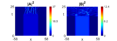
The Maxwell point between and is remarkable since and are not related by any symmetry. We shall refer to such DWs as “asymmetric domain walls” and discuss them qualitatively as part of our classification program. An example time evolution in Eq. (1) is shown in Fig. 1 with the initial condition being two asymmetric DWs assembled back-to-back to satisfy the periodic boundary conditions in . We observe that the asymmetric DW is a valid solution of Eq. (1) and persists for a short time before instability develops. We stress that Fig. 1 only provides a preliminary example of asymmetric DWs, and we cannot rule out the possible existence of stable asymmetric DWs with other parameter choices. A systematic study of asymmetric DWs and related solutions is left as future work.
By contrast, the Maxwell point between and are more natural since and can be related by exchanging and in Eq. (5), although this exchange symmetry is inexact for generic parameter choices. In this case, Eq. (15) yields the following condition for the existence of heteroclinic orbits between and :
| (16) |
This heteroclinic condition defines four points on the unit circle in the -plane, but the existence conditions for both and in Eq. (7) choose a unique point depending on the signs of and . Moreover, the spatially hyperbolic conditions for both and require the defocusing conditions and and the immiscibility condition . The latter reduces to the immiscibility condition in the BEC setting when [66]. In this setting, DWs are well studied both physically [67] and mathematically [68].
To complete the classification of DWs between and , we express the heteroclinic condition in Eq. (16) in the original traveling wave parameter space using the Galilean transformation in Eq. (6). Since Eq. (16) defines a half-line from the origin in the -plane, Eqs. (6,16) define a 2D angular sector denoted by in the 3D -space where by definition. For generic choices of the CNLS parameters , the sector has a 2D projection onto the -plane, so there is a unique Maxwell point with as the bifurcation parameter and fixed:
| (17) |
However, for special choices of satisfying
| (18) |
the sector is perpendicular to the -plane, so must satisfy Eq. (16) with replaced by , and is arbitrary at fixed . This applies most notably to symmetric CNLS (, , ) [56, 57, 58, 39, 65], and more generally to a codimension-1 subset of the CNLS parameter space defined by Eq. (18).
We stress that asymmetric DWs between and and symmetric DWs between and cannot be related by continuous deformation of parameters, namely they are homotopically nonequivalent. To see this, we first define the focusing and defocusing regimes for Eq. (8) with general coefficients. At fixed parameters, we call Eq. (8) focusing if the equilibrium is spatially hyperbolic, and defocusing if at least one of the two equilibria, and , is spatially hyperbolic. By this definition, Eq. (8) may be focusing, defocusing, or neither, but not both. Thus, asymmetric DWs only exist in the focusing regime, while symmetric DWs only exist in the defocusing regime. Note that prior work on DWs between and in binary BECs define asymmetric and symmetric DWs depending on the symmetry of their spatial profiles [69, 73]. In our language, both are symmetric DWs that are typically homotopically equivalent.
After classifying heteroclinic orbits in Eq. (5), the next question is whether these orbits persist into Eq. (2) with the restriction in Eq. (4) removed. Since equilibria of Eq. (2) correspond to plane waves in Eq. (5), the Maxwell point between two equilibria in Eq. (2) can be determined as the Maxwell point between two plane waves in Eq. (5) using the Hamiltonian in Eq. (14). Thus, one may naively expect the existence of a heteroclinic orbit between the and equilibria in Eq. (2) at this Maxwell point. However, the time evolution in Eq. (1) of an initial step between arbitrary and plane waves typically yields a DW with two dispersive shock waves respectively to the left and to the right of the DW, and this DW does satisfy the restriction in Eq. (4) even if the initial condition does not. A proper treatment of this time evolution requires modulation theory [54, 55], but here we tentatively conclude that the restriction in Eq. (4) is indispensable for the existence of DWs.
4 Vector solitons
In this section, we first seek vector solitons as homoclinic orbits to an equilibrium in the real ODE in Eq. (8), and then extend this solution family into the complex ODE in Eq. (2). Since Eq. (8) is reversible under the action in Eq. (9), the 4D phase space of Eq. (8) is symmetric with respect to four 2D sections with specified by two conditions:
| (19) |
A homoclinic orbit to an equilibrium requires a transverse intersection between the 2D stable manifold of the equilibrium and a 2D section . This intersection generally exists on a codimension-0 subset of the parameter space, so any spatially hyperbolic equilibrium may support a homoclinic orbit [72]. In principle, all possible homoclinic orbits to an equilibrium can be obtained by computing the 2D stable manifold of this equilibrium, but invariant manifolds are generally hard to compute due to their complicated geometry. In practice, homoclinic orbits are often found using numerical continuation in a bifurcation parameter starting from an initial guess.
The initial guess for numerical continuation could be an analytical ansatz, but a more systematic approach is to identify bifurcation points where a solution branch originates or terminates. Thus, our analysis centers upon three codimension-1 mechanisms to generate vector solitons in Eq. (8) from local and global bifurcation theory.
4.1 Heteroclinic cycles
Perhaps the most important type of global bifurcation for homoclinic orbits is the Maxwell point for heteroclinic orbits in Section 3, since a heteroclinic orbit and its symmetric partner can be assembled back-to-back to form a special type of homoclinic orbit known as a heteroclinic cycle [50]. A heteroclinic orbit from equilibrium to equilibrium , denoted by , has an even partner and an odd partner , for either component. A heteroclinic orbit can always be assembled with its even partner to form a heteroclinic cycle , but it can only be assembled with its odd partner to form a heteroclinic cycle when since , not when since .
Two asymmetric DWs between and can form a heteroclinic cycle with embedded in , which is an extended BB soliton, or a heteroclinic cycle with embedded in , which is an extended DD soliton. The extended BB soliton has multiplicity 1 and is always even-even; see the initial condition of Fig. 1 for an example. The extended DD soliton has multiplicity 4 and can be even-even, even-odd, odd-even, or odd-odd.
Two symmetric DWs between and can form a heteroclinic cycle with embedded in , or one with embedded in , both of which are extended DB solitons. An extended DB soliton has multiplicity 2 and can be even-even or odd-even.
Overall, an extended vector soliton with dark components has multiplicity since a dark component can be even or odd. Besides, this multiplicity persists when the extended vector soliton is numerically continued, at least near the Maxwell point. Hence, we shall refer to a vector soliton thus obtained near the Maxwell point as a quasi-extended vector soliton. Such a vector soliton can inherit certain properties from the underlying DW even if its spatial profile is not fully extended.
4.2 Local bifurcations
In addition to global bifurcations that only occur in certain parameter regimes, e.g., the immiscible regime, Eq. (8) also exhibits local bifurcations that can occur in virtually all parameter regimes. A codimension-1 local bifurcation occurs when an equilibrium becomes spatially hyperbolic, namely one or two pairs of spatial eigenvalues given by Eq. (13) leave the imaginary axis, as a bifurcation parameter, say , varies. A codimension-2 bifurcation occurs when two codimension-1 bifurcations collide, or the nature of a codimension-1 bifurcation changes, e.g., from supercritical to subcritical, as two bifurcation parameters, say and one of , vary.
There are two types of codimension-1 local bifurcations that can yield homoclinic orbits [72]. The first type is the Turing or Hamiltonian-Hopf bifurcation, where four purely imaginary eigenvalues collide pairwise on the imaginary axis to yield a complex quartet of eigenvalues. The second type is the pitchfork bifurcation, where two purely imaginary eigenvalues collide at the origin to yield two real eigenvalues. Note that the pitchfork bifurcation reflects the up-down symmetry of Eq. (8), and a saddle-node bifurcation would occur without such symmetries.
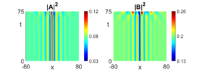
The defining feature of the Turing bifurcation is its ability to generate spatially periodic states. As such, it has played a key role for pattern formation in nonlinear dissipative PDEs for decades. More recently, the subcritical Turing bifurcation has been much studied since it can generate spatially localized states with rich bifurcation structures [50]. We have found that a subcritical Turing bifurcation can occur in Eq. (8), but only on the equilibrium. This bifurcation creates two branches of even-even localized states whose spatial profiles relative to differ by an overall sign to leading nontrivial order. We shall refer to localized states near this bifurcation as weakly nonlinear “Turing solitons” and discuss them qualitatively as part of our classification program. An example time evolution in Eq. (1) is shown in Fig. 2 with the initial condition being a weakly nonlinear Turing soliton. We observe that the Turing soliton is a valid solution of Eq. (1) and persists for a short time before instability develops. We stress that Fig. 2 only provides a preliminary example of Turing solitons, and we cannot rule out the possible existence of stable Turing solitons with other parameter choices. A systematic study of Turing solitons and related solutions is left as future work.
Generally, we define a Turing soliton as any vector soliton embedded in with an oscillatory tail due to the complex spatial eigenvalues of . A component of a Turing soliton can be called dark if the center is a dip or antidark if the center is a hump. For example, the initial condition of Fig. 2 can be called a DAD Turing soliton since the center of the () component is a hump and the center of the () component is a dip. However, apart from the central hump or dip, a DAD Turing soliton has an infinite number of humps and dips in its oscillatory tail. If the DAD Turing soliton is weakly nonlinear, then the oscillatory tail can have a larger L2-norm than the central hump or dip. By contrast, a normal DAD soliton has a monotonic tail due to the real spatial eigenvalues of , so the central hump or dip generally dominates.
In a dynamical system with an up-down symmetry, there is always an equilibrium at zero, and the pitchfork bifurcation causes two nonzero equilibria related by the up-down symmetry to emerge from the zero equilibrium as a parameter varies. A pitchfork bifurcation in Eq. (8) can occur on a zero component regardless of whether the other component is zero or nonzero. Thus, or can bifurcate from , and can bifurcate from or . For the latter, the bifurcation parameter can be chosen as either or . However, for the former, the bifurcation parameter can only be chosen as the that the or equilibrium depends on. Thus, there are no ambiguities if the value where an equilibrium bifurcates from an equilibrium is denoted by . For example, the value where bifurcates from is denoted by . A network can be constructed to visualize these pitchfork bifurcations with the nodes representing the four equilibria and the edges representing the bifurcation points; see Fig. 3. Note that the two types of Maxwell points in Section 3 represented on this network would occupy the two diagonal edges.
Analytical expressions can be derived for weakly nonlinear vector solitons near these pitchfork bifurcation points using asymptotic analysis. The details of these rather standard calculations will be omitted, but we note that asymptotic analyses near different pitchfork bifurcations always yield the same second-order ODE, known as the normal form, only with different coefficients [72]. This normal form ODE can admit, in different parameter regimes, either an even homoclinic orbit to the zero equilibrium, or an odd homoclinic orbit connecting the two nonzero equilibria related by the up-down symmetry.
Near or , one of the two components remains zero past the bifurcation point, so we obtain the pitchfork bifurcation in the scalar NLS equation that yields the well-known branches of exact solutions. The even homoclinic orbit corresponds to scalar bright solitons in the focusing regime with a sech shape, while the odd homoclinic orbit corresponds to scalar dark solitons in the defocusing regime with a tanh shape. These branches of exact solutions are not vector solitons and so will not be shown explicitly. However, one can identify codimension-1 bifurcation points on the branch of scalar dark solitons from the perspective of quantum mechanics and obtain branches of DB solitons whose bright components can have one or more humps [46, 47]. In Section 4.3, we shall present another application of exact solutions to scalar NLS by “lifting” them to codimension-1 families of exact solutions to Eq. (8) that can be numerically continued directly into vector solitons.
The pitchfork bifurcation point on is given by
| (20) |
Near , we assume that , where , and use the expansion
| (21) |
where is the perturbed equilibrium, and is the -dependent part that determines the spatial profile of the vector soliton. The pitchfork bifurcation is subcritical when . In this case, the leading nontrivial order for is and contains the even homoclinic orbit of the normal form, which is a bright component of the vector soliton:
| (22) |
The pitchfork bifurcation is supercritical when . In this case, the leading nontrivial order for is and contains the odd homoclinic orbit of the normal form, which is a dark component of the vector soliton:
| (23) |
In both the subcritical and the supercritical cases, the leading nontrivial order for is and contains an even localized profile “induced” by :
| (24) |
where . In the subcritical case, is a dark component when , and an antidark component when . Thus, the former is a DB soliton, while the latter is a BAD soliton. In the supercritical case, is an antidark component when , and a dark component when . Thus, the former is a DAD soliton, while the latter is a DD soliton. In the BEC setting, the existence of these four types of vector solitons is established from the perspective of quantum mechanics in Ref. [39], where the antidark concept is first introduced. In the physics community, DAD solitons are better known as magnetic solitons, which are actively studied theoretically [74, 75] and experimentally [76].
The pitchfork bifurcation point on is given by
| (25) |
Near , we can again assume , use the expansion in Eq. (21), and obtain the four types of vector solitons similarly to the case. These solutions are summarized next but not shown explicitly. The pitchfork bifurcation is subcritical when . In this case, is an bright component that is even. The pitchfork bifurcation is supercritical when . In this case, is an dark component that is odd. In both cases, is an dark or antidark component that is even. In the subcritical case, is dark if and antidark if . These are respectively a DB soliton and a BAD soliton. In the supercritical case, is antidark if and dark if . These are respectively a DAD soliton and a DD soliton. Notably, these DD or DAD solitons bifurcating from may coexist with the DD or DAD solitons bifurcating from , but these two branches are distinct since they have opposite parities in both components.
The pitchfork bifurcation is the fundamental bifurcation connecting the four equilibria as visualized in Fig. 3. Thus, after analyzing the codimension-1 bifurcations, it is also useful to identify the codimension-2 bifurcations. To identify the codimension-2 pitchfork bifurcation point for any equilibrium from Fig. 3, one can first identify the node representing this equilibrium and then equate the two codimension-1 points represented by the two edges meeting at this node. Since a codimension-2 point selects a triangle in Fig. 3 that contains a diagonal edge, it can provide valuable insights into the interplay between DWs and vector solitons. We shall identify the codimension-2 points but leave a detailed study as future work.
For , there are no nontrivial codimension-2 points.
For , Eqs. (20,25) imply that the codimension-2 point is . This is the miscible-immiscible transition point, which separates the miscible regime featuring DD solitons and the immiscible regime featuring symmetric DWs between and [38].
For , Eq. (20) and imply that the codimension-2 point is . For , Eq. (25) and imply that the codimension-2 point is . These are focusing-defocusing transition points, which separate the focusing regime featuring asymmetric DWs between and and the defocusing regime featuring DB solitons embedded in either or .
4.3 Exact solutions
As an application of exact solutions to scalar NLS including scalar bright and dark solitons, we lift them to exact solutions to Eq. (8) by requiring a scalar soliton multiplied by a constant amplitude vector to satisfy Eq. (8).
To find scalar bright solitons with vector amplitudes, we substitute the following ansatz into Eq. (8):
| (26) |
where without loss of generality. This yields the following consistency condition:
| (27) |
while the soliton parameters are
To find scalar dark solitons with vector amplitudes, we substitute the following ansatz into Eq. (8):
| (28) |
where without loss of generality. This yields the same consistency condition as the bright case given by Eq. (27), while the soliton parameters are
Arguably, scalar bright or dark solitons with vector amplitudes are not true BB or DD vector solitons. However, they are reversible homoclinic orbits that happen to have exact analytical expressions when the consistency condition in Eq. (27) is satisfied. Once they are numerically continued such that Eq. (27) is no longer satisfied, they become true BB or DD vector solitons whose profiles cannot be exactly a sech or a tanh function. Thus, we shall consider the exact solutions themselves as true vector solitons and call them scalar BB and DD solitons.
4.4 Summary of real vector solitons
After identifying the three codimension-1 mechanisms for generating vector solitons in Eq. (8), we can group these vector solitons by their types and possible parities; see Table 1. Overall, a bright or an antidark component is always even, while a dark component can be either even or odd. Any codimension-1 family of vector solitons in Table 1 can be numerically continued into a codimension-0 family of vector solitons, namely a 2-parameter family in or equivalently a 3-parameter family in using the Galilean transformation in Eq. (6). These codimension-0 families of vector solitons may not be distinct since two vector solitons of the same type and parity but generated by different mechanisms could be parametrically related in Eq. (8).
| Type of vector soliton | Possible parities |
|---|---|
| Heteroclinic cycles | |
| (Quasi-)Extended BB | 1 EE |
| (Quasi-)Extended DD | 1 EE + 1 EO + 1 OE + 1 OO |
| (Quasi-)Extended DB | 1 EE + 1 OE |
| Local bifurcations | |
| Weakly nonlinear DB | 1 EE |
| Weakly nonlinear BAD | 1 EE |
| Weakly nonlinear DD | 1 EO/OE |
| Weakly nonlinear DAD | 1 OE |
| Weakly nonlinear Turing | 2 EE |
| Exact solutions | |
| Scalar BB | 1 EE |
| Scalar DD | 1 OO |
BAD, DAD, and Turing solitons can only be generated by local bifurcations, not heteroclinic cycles or exact solutions. Nonetheless, since Turing, DD, and DAD solitons share the background, a Turing soliton could be parametrically related to a DD or a DAD soliton via the so-called Belyakov-Devaney point, where the spatial eigenvalues given by Eq. (13) transition from a complex quartet of eigenvalues to four real eigenvalues by colliding pairwise on the real axis, or vice versa [72].
There are two types of BB solitons including extended and scalar BB solitons. Both are even-even, so they could be parametrically related.
There are two types of DB solitons including extended and weakly nonlinear DB solitons. The former can be even-even or odd-even, while the latter are even-even. Thus, even-even extended DB solitons could be parametrically related to weakly nonlinear DB solitons.
There are three types of DD solitons including extended, weakly nonlinear, and scalar DD solitons. Extended DD solitons can have all four possible parities. Weakly nonlinear DD solitons are either even-odd or odd-even, say even-odd. Scalar DD solitons are odd-odd. Thus, even-odd extended DD solitons could be parametrically related to weakly nonlinear DD solitons, while odd-odd extended DD solitons could be parametrically related to scalar DD solitons.
4.5 Complex vector solitons
Once we have a 3-parameter family of real homoclinic orbits in in Eq. (8), we can remove the restriction in Eq. (4) and numerically continue these orbits in to obtain a 5-parameter family of complex homoclinic orbits in Eq. (2). Although these orbits are different solutions to the ODE in Eq. (2), they do not always yield different vector solitons in the PDE in Eq. (1).
Consider a numerical continuation from to ; the case is similar. To identify which ODE solutions yield the same vector soliton in the PDE, we observe that the component of a vector soliton can be rewritten as where
| (29) |
and, recalling that ,
| (30) |
Thus, the two solution families, at and at , yield the same family of vector solitons.
If is homoclinic to the equilibrium, namely dark or antidark, then is homoclinic to a nonzero plane wave. Since the numerical continuation from to yields a solution family homoclinic to the equilibrium, this solution family cannot be equivalent to , so this continuation must yield a different family of vector solitons. Notably, this continuation might connect two branches of real vector solitons with different parities.
However, if is homoclinic to the equilibrium, namely bright, then is also homoclinic to the equilibrium. Since the numerical continuation from to also yields a solution family homoclinic to the equilibrium, this solution family must be equivalent to with the equivalence given by Eqs. (29–30), so this continuation does not yield a different family of vector solitons.
The nontrivial continuation in the wavenumber for a dark or antidark component, but not a bright component, is perhaps best known in the scalar NLS equation, where scalar bright solitons have two parameters including the group velocity and the frequency, while scalar dark solitons have three parameters including the group velocity, the frequency, and the wavenumber [21]. The profile of a scalar dark soliton is a real tanh function plus an imaginary constant , where is the darkness parameter with for a black soliton and for a gray soliton. In our language, a black soliton is a real scalar dark soliton, a gray soliton is a complex scalar dark soliton, and the former can be continued in the wavenumber to obtain the latter.
The continuation in the wavenumber of a dark or antidark component from real to complex can always be performed numerically, but a complex dark component may also be expressible analytically as exemplified by the scalar NLS equation. In the CNLS equation, one can similarly generalize a black component described by a real tanh function to a gray component by adding an imaginary constant. There are three types of real vector solitons in Table 1 with such a black component including weakly nonlinear DD, weakly nonlinear DAD, and scalar DD solitons. For the first two types, the component in Eq. (23) can be generalized from black to gray similarly to scalar NLS, which will not be shown explicitly. For the third type, both components can be generalized from black to gray by adding an imaginary vector to Eq. (28):
| (31) |
where without loss of generality, and . Substituting this ansatz into Eq. (2) with the following shorthand notations for its coefficients
we obtain the following consistency condition
while the soliton parameters are
Thus, the 2-parameter family of black-black solitons in Eq. (28) can be generalized to the 4-parameter family of gray-gray solitons in Eq. (31). The two darkness parameters and become nonzero respectively when and become nonzero, so this generalization is essentially a continuation in , or equivalently the two wavenumbers . The general family of complex DD solitons have five parameters and can be obtained from this family of gray-gray solitons by numerical continuation in , or equivalently , such that the above consistency condition is violated.
Although a bright component cannot be non-trivially continued in the wavenumber like a dark or an antidark component, the latter cannot be non-trivially multiplied by a constant phase factor or like the former for vector soliton collisions. This is because in a collision between two vector soliton respectively located on the left and on the right, the left and right dark or antidark components must have matching phases, while the left and right bright components can have any phases. Moreover, the left and right bright components can also have different frequencies, so one can expect richer dynamics when a soliton collision involves at least one bright component. If the component of a vector soliton is bright, then we define the polarization of this vector soliton as the phase difference regardless of whether the component is bright, dark, or antidark.
5 Numerical continuation
Since vector solitons are reversible homoclinic orbits, only half of the soliton profile needs to be numerically continued, say the right half. Thus, we can choose a domain with large, such that is the center of the soliton and is the tail of the soliton. At , we can impose Neumann boundary conditions such that the tail decays to the background equilibrium. At , we must impose boundary conditions required by the reversibility symmetry of the soliton in question.
To numerically continue a real vector soliton with the reversibility in Eq. (9), we must impose at the boundary conditions in Eq. (19), which depend on the parities of the two components. As stated earlier, to convert a real vector soliton to a complex vector soliton with the reversibility in Eq. (3), any odd component must be multiplied by . To numerically continue a complex vector soliton with the reversibility , we must impose at the boundary conditions corresponding to the symmetric section given explicitly by
| (32) |
As an application of our classification program, we consider an example with the CNLS parameters , , , , , and . This parameter combination is in the defocusing regime relevant to BECs, and the immiscibility condition is satisfied. Thus, the and equilibria can be both spatially hyperbolic, and a DW may form at the Maxwell point in Eq. (17). An example combination of the traveling wave parameters satisfying both conditions is . To compute a DW profile at the Maxwell point, we make Eq. (8) the steady state of a dissipative PDE and evolve an initial step between and in this PDE to reach the steady state, but there are other numerical methods available.
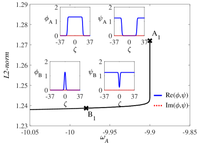
Once a DW profile between and is computed, it can be treated as half of the profile of an extended DB soliton and numerically continued into a codimension-0 family of real vector solitons. As listed in Table 1, an extended DB soliton has two possible parities including even-even and odd-even. We shall focus on the former and leave the latter as future work. Thus, we impose even-even boundary conditions at , namely Eq. (19) with , Neumann boundary conditions at , and numerically continue the DW in one of the traveling wave parameters , say . We use the software AUTO-07p [77] for all numerical continuations in this paper, but other software can also be used. The bifurcation diagram is shown in Fig. 4 with the profiles of the accompanying solutions shown in the insets. Note that although the full soliton profile is plotted, only half of the profile is numerically continued. The starting point is the extended DB soliton at whose profile is shown as and and consists of two DWs. As varies, the two DWs “merge” into a generic real DB soliton at whose profile is shown as and . Although not shown explicitly in Fig. 4, this branch of even-even DB solitons terminates at the pitchfork bifurcation point on the equilibrium.
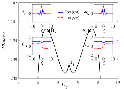
As discussed in Section 4.5, a 3-parameter family of real DB solitons in can be numerically continued in the wavenumber of the dark component into a 4-parameter family of complex DB solitons. A key motivation to compute complex vector solitons is to study interactions (collisions) involving such solitons, during which the interacting solitons must share the same plane wave background. Thus, we impose reversible boundary conditions in Eq. (32) at , Neumann boundary conditions at , and numerically continue complex DB solitons in with fixed rather than in with fixed. The bifurcation diagram is shown in Fig. 4 with the profiles of the accompanying solutions shown in the insets. The starting point is the real DB soliton at in Fig. 4. As increases, one obtains a complex DB soliton at whose profile is shown as and . As decreases, one obtains a complex DB soliton at whose profile is shown as and . The bifurcation diagram is symmetric with respect to and the solution profiles at and are related by complex conjugation. This is expected since Eq. (2) to the left and to the right of differ only in the sign of the coefficient of .
Extended DB solitons formed by two DWs are well studied in the optics setting where they are often called domain wall solitons [56, 57, 58, 59], and in the BEC setting where they are sometimes called bubble droplets [69]. The above example shows that DWs and DB solitons can be parametrically related in the immiscible regime of the asymmetric CNLS equation relevant to BECs. An interesting prospect is to deduce analytically the properties of quasi-extended DB solitons near the Maxwell point from the properties of the underlying DW.
6 Collisions between two polarized dark-bright solitons
In Section 5, we have obtained a 4-parameter family of complex DB solitons in with the component being dark and the component being bright. As discussed in Section 4.5, the bright component can be multiplied by a constant phase factor to yield a 5-parameter family of polarized DB solitons in for soliton collisions. In such collisions, the 2 parameters must be the same between the two colliding solitons such that the solitons share the same plane wave background, but the other 3 parameters can be different. Among these, must be different for the collision to occur, will be taken as the same for simplicity, and we shall focus on the effect of different . We shall denote as the polarization recalling that and for the dark component . In the BEC setting, it is well known that collisions between two polarized DB solitons can yield a mass exchange between the two bright components [37]. We shall examine this mass exchange in the immiscible regime through a numerical example.
To reduce radiation for soliton collisions, we consider an example with the CNLS parameters , , and , which differs from the defocusing Manakov system only by adding 1 to . Apart from near integrability, this example and the example in Section 5 have similar bifurcation structures since both belong to the immiscible regime. A DW exists at the Maxwell point . A real DB soliton can be found by numerical continuation of the DW to similarly to Fig. 4. A family of complex DB solitons sharing the same plane wave background can be obtained by numerical continuation of the real DB soliton in similarly to Fig. 4. These two bifurcation diagrams will not be shown explicitly since they are similar to Fig. 4(a,b). We shall call the group velocity of the real DB soliton . For soliton collisions, we shall choose two complex DB solitons with values symmetric with respect to similarly to Fig. 4, which are respectively called . Thus, these two solitons have opposite velocities in the frame comoving with velocity , and the two soliton profiles are related by complex conjugation.
The initial conditions to be time-evolved in Eq. (1) consist of these two complex DB solitons respectively located on the left and on the right. The left bright component is multiplied by , and the right bright component is multiplied by , where are the polarizations of the two colliding solitons. We can set without loss of generality and explore the effect of varying . The collision dynamics for two choices of are shown in Fig. 5. As expected, the case yields no mass exchange as shown in Fig. 5. To explore , we choose , and observe a mass exchange as shown in Fig. 5. Note that both collisions produce negligible radiation compared with the solitons, which is consistent with the near integrability of Eq. (1).
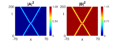
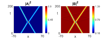
We shall examine this mass exchange in terms of both soliton parameters and soliton profiles.
In terms of soliton parameters, the 2 parameters of the dark component, , cannot change since the incoming and outgoing solitons must share the same plane wave background. However, the soliton velocity , which is a shared parameter between both components, can change as shown in Fig. 5. The 2 parameters of the bright component, ), can also change.
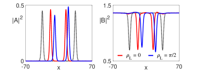
In terms of soliton profiles, the profiles of both components can change. As shown in Fig. 5, there is a visible difference in the amplitudes of both components after the polarized collision in Fig. 5 (blue) compared with either after the unpolarized collision in Fig. 5 (red) or before collisions (black-dashed). Thus, in terms of soliton profiles alone, it is tempting to describe the mass exchange as an energy transfer, but the latter usually applies between two bright components, not between a bright component and a dark one.
Overall, the change in soliton profiles in both components results from the change in the 2 soliton parameters , as exemplified by Fig. 4. The polarizations of the two solitons can also change, but they do not affect the soliton profiles. Thus, the mass exchange is better described by the change in soliton parameters than the change in soliton profiles, although the soliton profiles are more visible than the soliton parameters.
We stress that Fig. 5 shows a collision between two generic DB solitons whose dark and bright components have comparable amplitudes. In such cases, the relative changes of the amplitudes of both components produced by the mass exchange are moderate as shown in Fig. 5. However, if either or both of the two colliding solitons are near bifurcation points, then their dark and bright components could have very different amplitudes. In such cases, the relative changes of the amplitudes of either or both components produced by the mass exchange could be very large or very small. The eigenfunctions in the spectra of vector solitons can yield valuable insights into the collision dynamics of these solitons in non-integrable regimes of Eq. (1); see e.g. Ref. [33] for the collision dynamics of BB solitons explained from this perspective.
7 Conclusion
In this paper, we have outlined a program to classify DWs and vector solitons in the 1D two-component CNLS equation without restricting the signs or magnitudes of any coefficients. The CNLS equation is reduced first to a complex ODE, and then to a real ODE after imposing a restriction. In the real ODE, we have identified four possible equilibria including ZZ, ZN, NZ, and NN, and analyzed their spatial stability. We have identified two types of DWs including asymmetric DWs between ZZ and NN and symmetric DWs between ZN and NZ. We have identified three mechanisms for generating vector solitons in the real ODE including heteroclinic cycles formed by assembling two DWs back-to-back, local bifurcations on the four equilibria, and exact solutions that are scalar solitons with vector amplitudes. Local bifurcations are further divided into the Turing bifurcation that generate Turing solitons and the pitchfork bifurcation that generates DB, BAD, DD, and DAD solitons. We have identified a 3D parameter space for real vector solitons and a 5D parameter space for complex vector solitons, and introduced a numerical continuation method to find these vector solitons. Our classification program applies not only to optics and BECs, but also to the general problem of two interacting quasi-monochromatic plane waves. Further solutions that can be incorporated into our classification program include those originating from secondary bifurcations or codimension-2 bifurcations.
As an application of our classification program, we have shown that real and complex DB solitons can be parametrically related to DWs in the immiscible regime of the CNLS equation relevant to BECs. We have also shown that in this regime, collisions between two polarized DB solitons typically feature a mass exchange that changes the frequencies and polarizations of the two bright components and the two soliton velocities.
Our classification program can be generalized to the -components CNLS equation for interacting quasi-monochromatic plane waves. This equation overlaps with the -component GPE for bosonic BECs [36] in certain parameter regimes. This equation has possible equilibria, so its complexity increases exponentially with .
Our classification program is also relevant to the 2D two-component CNLS equation. In the BEC setting, the 2D GPE can exhibit radial solutions like vortices due to the radial symmetry of the Laplacian [36]. However, for two interacting quasi-monochromatic plane waves in 2D, the dispersion relation of either plane wave can be either elliptic or hyperbolic, so the linear part of the 2D CNLS equation generally lacks radial symmetry. Nonetheless, the 2D CNLS equation can be reduced along any line to the 1D CNLS equation that we studied, so 1D solitons in the latter correspond to 2D line solitons in the former.
We have applied our classification program to DWs and DB solitons in the homogeneous GPE, but the effects of a trapping potential on such solutions can also be remarkable. Stable pinning of DWs near maxima of the potential is shown both physically [65] and mathematically [68]. A plethora of DB solitons are found with a harmonic trap using numerical continuation in recent studies [78, 79]. The GPE in the immiscible regime with a trapping potential continues to provide a great venue for further explorations of DWs and DB solitons.
Acknowledgement
YM acknowledges support from a Vice Chancellor’s Research Fellowship at Northumbria University. We thank Gennady El, Benoit Huard, Antonio Moro, and Matteo Sommacal for their helpful comments.
References
References
- [1] Catherine Sulem and Pierre-Louis Sulem. The nonlinear Schrödinger equation: self-focusing and wave collapse, volume 139. Springer Science & Business Media, 2007.
- [2] Mark J Ablowitz, B Prinari, and A D Trubatch. Discrete and continuous nonlinear Schrödinger systems, volume 302. Cambridge University Press, 2004.
- [3] A Shabat and V Zakharov. Exact theory of two-dimensional self-focusing and one-dimensional self-modulation of waves in nonlinear media. Soviet physics JETP, 34(1):62, 1972.
- [4] Mark J Ablowitz and Harvey Segur. Solitons and the inverse scattering transform, volume 4. Siam, 1981.
- [5] Sergei V Manakov. On the theory of two-dimensional stationary self-focusing of electromagnetic waves. Soviet Physics-JETP, 38(2):248–253, 1974.
- [6] VE Zakharov and SV Manakov. The theory of resonance interaction of wave packets in nonlinear media. Zh. Eksp. Teor. Fiz., 69(5):1654–1673, 1975.
- [7] C Menyuk. Nonlinear pulse propagation in birefringent optical fibers. IEEE Journal of Quantum electronics, 23(2):174–176, 1987.
- [8] Zhigang Chen, Mordechai Segev, Tamer H Coskun, Demetrios N Christodoulides, and Yuri S Kivshar. Coupled photorefractive spatial-soliton pairs. JOSA B, 14(11):3066–3077, 1997.
- [9] Elena A Ostrovskaya, Yuri S Kivshar, Zhigang Chen, and Mordechai Segev. Interaction between vector solitons and solitonic gluons. Optics letters, 24(5):327–329, 1999.
- [10] Sergey K Ivanov, Yaroslav V Kartashov, Alexander Szameit, Lluis Torner, and Vladimir V Konotop. Vector topological edge solitons in floquet insulators. ACS Photonics, 7(3):735–745, 2020.
- [11] Padma K Shukla, Ioannis Kourakis, Bengt Eliasson, Mattias Marklund, and Lennart Stenflo. Instability and evolution of nonlinearly interacting water waves. Physical Review Letters, 97(9):094501, 2006.
- [12] Mark J Ablowitz and Theodoros P Horikis. Interacting nonlinear wave envelopes and rogue wave formation in deep water. Physics of Fluids, 27(1):012107, 2015.
- [13] SD Griffiths, RHJ Grimshaw, and KR Khusnutdinova. Modulational instability of two pairs of counter-propagating waves and energy exchange in a two-component system. Physica D: Nonlinear Phenomena, 214(1):1–24, 2006.
- [14] Lev Pitaevskii and Sandro Stringari. Bose-Einstein condensation and superfluidity, volume 164. Oxford University Press, 2016.
- [15] Panayotis G Kevrekidis, Dimitri J Frantzeskakis, and Ricardo Carretero-González. The defocusing nonlinear Schrödinger equation: from dark solitons to vortices and vortex rings. SIAM, 2015.
- [16] Vladimir E Zakharov and EI Schulman. To the integrability of the system of two coupled nonlinear schrödinger equations. Physica D: Nonlinear Phenomena, 4(2):270–274, 1982.
- [17] R Sahadevan, KM Tamizhmani, and M Lakshmanan. Painleve analysis and integrability of coupled non-linear schrodinger equations. Journal of Physics A: Mathematical and General, 19(10):1783, 1986.
- [18] Deng-Shan Wang, Da-Jun Zhang, and Jianke Yang. Integrable properties of the general coupled nonlinear schrödinger equations. Journal of Mathematical Physics, 51(2):023510, 2010.
- [19] Norman J Zabusky and Martin D Kruskal. Interaction of” solitons” in a collisionless plasma and the recurrence of initial states. Physical review letters, 15(6):240, 1965.
- [20] Philip G Drazin and Robin S Johnson. Solitons: an introduction, volume 2. Cambridge university press, 1989.
- [21] Mark J Ablowitz. Nonlinear dispersive waves: asymptotic analysis and solitons, volume 47. Cambridge University Press, 2011.
- [22] DJ Kaup and BA Malomed. Soliton trapping and daughter waves in the manakov model. Physical Review A, 48(1):599, 1993.
- [23] R Radhakrishnan, M Lakshmanan, and J Hietarinta. Inelastic collision and switching of coupled bright solitons in optical fibers. Physical Review E, 56(2):2213, 1997.
- [24] S Stalin, R Ramakrishnan, M Senthilvelan, and M Lakshmanan. Nondegenerate solitons in manakov system. Physical review letters, 122(4):043901, 2019.
- [25] DN Christodoulides. Black and white vector solitons in weakly birefringent optical fibers. Physics Letters A, 132(8-9):451–452, 1988.
- [26] VV Afanasyev, Yu S Kivshar, VV Konotop, and VN Serkin. Dynamics of coupled dark and bright optical solitons. Optics letters, 14(15):805–807, 1989.
- [27] Yuri S Kivshar and Sergei K Turitsyn. Vector dark solitons. Optics letters, 18(5):337–339, 1993.
- [28] R Radhakrishnan and M Lakshmanan. Bright and dark soliton solutions to coupled nonlinear schrodinger equations. Journal of Physics A: Mathematical and General, 28(9):2683, 1995.
- [29] Adrian P Sheppard and Yuri S Kivshar. Polarized dark solitons in isotropic kerr media. Physical Review E, 55(4):4773, 1997.
- [30] Q-Han Park and HJ Shin. Systematic construction of multicomponent optical solitons. Physical Review E, 61(3):3093, 2000.
- [31] Barbara Prinari, Mark J Ablowitz, and Gino Biondini. Inverse scattering transform for the vector nonlinear schrödinger equation with nonvanishing boundary conditions. Journal of mathematical physics, 47(6):063508, 2006.
- [32] Jianke Yang. Classification of the solitary waves in coupled nonlinear schrödinger equations. Physica D: Nonlinear Phenomena, 108(1-2):92–112, 1997.
- [33] Jianke Yang and Yu Tan. Fractal structure in the collision of vector solitons. Physical review letters, 85(17):3624, 2000.
- [34] Noel F Smyth and William L Kath. Radiative losses due to pulse interactions in birefringent nonlinear optical fibers. Physical Review E, 63(3):036614, 2001.
- [35] Marc Haelterman and AP Sheppard. Bifurcations of the dark soliton and polarization domain walls in nonlinear dispersive media. Physical Review E, 49(5):4512, 1994.
- [36] PG Kevrekidis and DJ Frantzeskakis. Solitons in coupled nonlinear schrödinger models: a survey of recent developments. Reviews in Physics, 1:140–153, 2016.
- [37] Th Busch and JR Anglin. Dark-bright solitons in inhomogeneous bose-einstein condensates. Physical review letters, 87(1):010401, 2001.
- [38] P Öhberg and L Santos. Dark solitons in a two-component bose-einstein condensate. Physical Review Letters, 86(14):2918, 2001.
- [39] PG Kevrekidis, HE Nistazakis, DJ Frantzeskakis, Boris A Malomed, and R Carretero-González. Families of matter-waves in two-component bose-einstein condensates. The European Physical Journal D-Atomic, Molecular, Optical and Plasma Physics, 28:181–185, 2004.
- [40] Christoph Becker, Simon Stellmer, Parvis Soltan-Panahi, Sören Dörscher, Mathis Baumert, Eva-Maria Richter, Jochen Kronjäger, Kai Bongs, and Klaus Sengstock. Oscillations and interactions of dark and dark–bright solitons in bose–einstein condensates. Nature Physics, 4(6):496–501, 2008.
- [41] C Hamner, JJ Chang, P Engels, and MA Hoefer. Generation of dark-bright soliton trains in superfluid-superfluid counterflow. Physical review letters, 106(6):065302, 2011.
- [42] D Yan, JJ Chang, C Hamner, PG Kevrekidis, P Engels, V Achilleos, DJ Frantzeskakis, R Carretero-González, and P Schmelcher. Multiple dark-bright solitons in atomic bose-einstein condensates. Physical Review A, 84(5):053630, 2011.
- [43] A Álvarez, J Cuevas, Francisco Romero Romero, C Hamner, JJ Chang, Peter Engels, Panayotis G Kevrekidis, and Dimitri J Frantzeskakis. Scattering of atomic dark–bright solitons from narrow impurities. Journal of Physics B: Atomic, Molecular and Optical Physics, 46(6):065302, 2013.
- [44] D Yan, F Tsitoura, PG Kevrekidis, and DJ Frantzeskakis. Dark-bright solitons and their lattices in atomic bose-einstein condensates. Physical Review A, 91(2):023619, 2015.
- [45] Alexander V Buryak, Yuri S Kivshar, and David F Parker. Coupling between dark and bright solitons. Physics Letters A, 215(1-2):57–62, 1996.
- [46] V Achilleos, DJ Frantzeskakis, and PG Kevrekidis. Beating dark-dark solitons and zitterbewegung in spin-orbit-coupled bose-einstein condensates. Physical Review A, 89(3):033636, 2014.
- [47] EG Charalampidis, PG Kevrekidis, DJ Frantzeskakis, and BA Malomed. Dark-bright solitons in coupled nonlinear schrödinger equations with unequal dispersion coefficients. Physical Review E, 91(1):012924, 2015.
- [48] Jack Xin. Front propagation in heterogeneous media. SIAM review, 42(2):161–230, 2000.
- [49] Wim Van Saarloos. Front propagation into unstable states. Physics reports, 386(2-6):29–222, 2003.
- [50] E Knobloch. Spatial localization in dissipative systems. Annual Review of Condensed Matter Physics, 6(1):325–359, 2015.
- [51] Boris A Malomed. Past and present trends in the development of the pattern-formation theory: domain walls and quasicrystals. Physics, 3(4):1015–1045, 2021.
- [52] Doug Jacobs, Bill McKinney, and Michael Shearer. Traveling wave solutions of the modified korteweg-devries-burgers equation. Journal of Differential Equations, 116(2):448–467, 1995.
- [53] Yuri S Kivshar and Boris A Malomed. Raman-induced optical shocks in nonlinear fibers. Optics letters, 18(7):485–487, 1993.
- [54] GA El and MA Hoefer. Dispersive shock waves and modulation theory. Physica D: Nonlinear Phenomena, 333:11–65, 2016.
- [55] GA El, MA Hoefer, and Michael Shearer. Dispersive and diffusive-dispersive shock waves for nonconvex conservation laws. SIAM Review, 59(1):3–61, 2017.
- [56] Marc Haelterman and AP Sheppard. Polarization domain walls in diffractive or dispersive kerr media. Optics Letters, 19(2):96–98, 1994.
- [57] Marc Haelterman and Adrian P Sheppard. Vector soliton associated with polarization modulational instability in the normal-dispersion regime. Physical Review E, 49(4):3389, 1994.
- [58] Boris A Malomed. Optical domain walls. Physical Review E, 50(2):1565, 1994.
- [59] Z Jovanoski, N Ansari, IN Towers, and RA Sammut. Exact domain-wall solitons. Physics Letters A, 372(5):610–612, 2008.
- [60] Stéphane Pitois, Guy Millot, and Stefan Wabnitz. Polarization domain wall solitons with counterpropagating laser beams. Physical review letters, 81(7):1409, 1998.
- [61] Stéphane Pitois, Guy Millot, Philippe Grelu, and Marc Haelterman. Generation of optical domain-wall structures from modulational instability in a bimodal fiber. Physical Review E, 60(1):994, 1999.
- [62] Marin Gilles, P-Y Bony, Jocelin Garnier, Antonio Picozzi, Massimiliano Guasoni, and Julien Fatome. Polarization domain walls in optical fibres as topological bits for data transmission. Nature Photonics, 11(2):102–107, 2017.
- [63] Constantinos Valagiannopoulos, Adilkhan Sarsen, and Andrea Alu. Angular memory of photonic metasurfaces. IEEE Transactions on Antennas and Propagation, 69(11):7720–7728, 2021.
- [64] Constantinos Valagiannopoulos. Multistability in coupled nonlinear metasurfaces. IEEE Transactions on Antennas and Propagation, 70(7):5534–5540, 2022.
- [65] Nir Dror, Boris A Malomed, and Jianhua Zeng. Domain walls and vortices in linearly coupled systems. Physical Review E, 84(4):046602, 2011.
- [66] Marek Trippenbach, Krzysztof Góral, Kazimierz Rzazewski, Boris Malomed, and YB Band. Structure of binary bose-einstein condensates. Journal of Physics B: Atomic, Molecular and Optical Physics, 33(19):4017, 2000.
- [67] Stéphane Coen and Marc Haelterman. Domain wall solitons in binary mixtures of bose-einstein condensates. Physical review letters, 87(14):140401, 2001.
- [68] Stan Alama, Lia Bronsard, Andres Contreras, and Dmitry E Pelinovsky. Domain walls in the coupled gross–pitaevskii equations. Archive for Rational Mechanics and Analysis, 215(2):579–610, 2015.
- [69] G Filatrella, Boris A Malomed, and Mario Salerno. Domain walls and bubble droplets in immiscible binary bose gases. Physical Review A, 90(4):043629, 2014.
- [70] GJ Roskes. Some nonlinear multiphase interactions. Studies in Applied Mathematics, 55(3):231–238, 1976.
- [71] Todd Kapitula and Keith Promislow. Spectral and dynamical stability of nonlinear waves, volume 457. Springer, 2013.
- [72] Alan R Champneys. Homoclinic orbits in reversible systems and their applications in mechanics, fluids and optics. Physica D: Nonlinear Phenomena, 112(1-2):158–186, 1998.
- [73] Boris A Malomed. New findings for the old problem: Exact solutions for domain walls in coupled real ginzburg-landau equations. Physics Letters A, 422:127802, 2022.
- [74] Chunlei Qu, Lev P Pitaevskii, and Sandro Stringari. Magnetic solitons in a binary bose-einstein condensate. Physical Review Letters, 116(16):160402, 2016.
- [75] Xiao Chai, Li You, and Chandra Raman. Magnetic solitons in an immiscible two-component bose-einstein condensate. Physical Review A, 105(1):013313, 2022.
- [76] A Farolfi, D Trypogeorgos, C Mordini, G Lamporesi, and G Ferrari. Observation of magnetic solitons in two-component bose-einstein condensates. Physical Review Letters, 125(3):030401, 2020.
- [77] Eusebius J Doedel, Alan R Champneys, Fabio Dercole, Thomas F Fairgrieve, Yu A Kuznetsov, B Oldeman, RC Paffenroth, B Sandstede, XJ Wang, and CH Zhang. AUTO-07P: Continuation and bifurcation software for ordinary differential equations. 2007.
- [78] Wenlong Wang, Li-Chen Zhao, Efstathios G Charalampidis, and Panayotis G Kevrekidis. Dark–dark soliton breathing patterns in multi-component bose–einstein condensates. Journal of Physics B: Atomic, Molecular and Optical Physics, 54(5):055301, 2021.
- [79] Wenlong Wang. Systematic solitary waves from their linear limits in two-component bose-einstein condensates with unequal dispersion coefficients. Journal of Physics B: Atomic, Molecular and Optical Physics, 56(13):135301, 2023.