Minimizing Quasi-Self-Concordant Functions
by Gradient Regularization of Newton Method

Abstract

We study the composite convex optimization problems with a Quasi-Self-Concordant smooth component. This problem class naturally interpolates between classic Self-Concordant functions and functions with Lipschitz continuous Hessian. Previously, the best complexity bounds for this problem class were associated with trust-region schemes and implementations of a ball-minimization oracle. In this paper, we show that for minimizing Quasi-Self-Concordant functions we can use instead the basic Newton Method with Gradient Regularization. For unconstrained minimization, it only involves a simple matrix inversion operation (solving a linear system) at each step. We prove a fast global linear rate for this algorithm, matching the complexity bound of the trust-region scheme, while our method remains especially simple to implement. Then, we introduce the Dual Newton Method, and based on it, develop the corresponding Accelerated Newton Scheme for this problem class, which further improves the complexity factor of the basic method. As a direct consequence of our results, we establish fast global linear rates of simple variants of the Newton Method applied to several practical problems, including Logistic Regression, Soft Maximum, and Matrix Scaling, without requiring additional assumptions on strong or uniform convexity for the target objective.

Keywords: Newton method, convex optimization, quasi-self-concordance, global complexities, global linear rates

1 Introduction

1.1 Motivation.

The Newton Method is a fundamental algorithm in Continuous Optimization. Involving in its computations the Hessian of the objective, it is considered to be a very powerful approach for solving numerical optimization problems. The modern theory of second-order optimization methods heavily relies on the notion of a problem class, that formally postulates our assumptions on the target objective function, and which determines the global complexity guarantees of the method.

Self-Concordant Functions.

Historically, one of the most successful descriptions of the Newton Method is the class of Self-Concordant functions [39], which has become a universal tool for constructing efficient Interior-Point Methods for non-linear Convex Optimization. A convex function $f$ is called Self-Concordant, if its third derivative is bounded with respect to the local norm induced by the Hessian. That is, for any $\bm{x}\in\operatorname{dom}f$ and arbitrary direction $\bm{u}$:

$$\begin{array}[]{rcl}D^{3}f(\bm{x})[\bm{u},\bm{u},\bm{u}]&\leq&M_{\mathfrak{sc}}{\langle}\nabla^{2}f(\bm{x})\bm{u},\bm{u}{\rangle}^{3/2},\end{array}$$ (1)

where $M_{\mathfrak{sc}}\geq 0$ is a certain constant (the parameter of self-concordance). Note that the exponent $3/2$ on the right hand side of (1) is the only viable choice, as dictated by the requirement for homogeneity in $\bm{u}$.

It seems that Self-Concordant functions are likely the most suitable problem class for characterizing the behaviour of the classic Newton Method [34]:

$$\begin{array}[]{rcl}\bm{x}_{k+1}&=&\bm{x}_{k}-\gamma_{k}\nabla^{2}f(\bm{x}_{k})^{-1}\nabla f(\bm{x}_{k}),\qquad k\geq 0.\end{array}$$ (2)

Here, $\gamma_{k}\in(0,1]$ is a damping parameter. The value $\gamma_{k}=1$ corresponds to the pure Newton step, which minimizes the full second-order Taylor polynomial of $f(\cdot)$ around the current point $\bm{x}_{k}$. However, the pure Newton step may not work globally, even if the objective functions is strongly convex (see, e.g., Example 1.4.3 in [11]).

An important feature of both definition (1) and the Newton step (2) is their invariance under affine transformation of variables: they do not depend on artificial norms, nor do they require a specific choice of the coordinate system.

For iterations of the damped Newton Method (2) minimizing a Self-Concordant function $f$, we can prove both super-fast local quadratic convergence (an affine-invariant variant of classical results about the local convergence of the Newton Method [18, 3, 25]), and global convergence, provided an appropriate choice of the damping parameter $\gamma_{k}$. Global convergence ensures that the method will reach the local region after a bounded number of iterations, starting from an arbitrary initial point $\bm{x}_{0}$. These global guarantees are essential for optimization algorithms, as the initial point may often be far from the solution’s neighbourhood. In the past decade, the study of the global behaviour of second-order methods has become one of the driving forces in the field, including analysis for Self-Concordant functions [17, 23, 38].

While serving as a powerful tool for minimizing the barrier function in Interior-Point Methods [39], it has become evident that the damping Newton scheme (2) and the corresponding problem class of Self-Concordant functions do not fit all modern applications. For more refined problem classes, it is possible to construct faster second-order schemes [17, 34]. Thus, to fulfil all practical needs, different assumptions must be considered.

Lipschitz Continuous Hessian.

In recent years, significant interest in second-order optimization has been linked to the Cubic Regularization of Newton Method with its excellent global complexity guarantees for a wide class of problems [40]. The core assumption of the Cubic Newton Method is that the Hessian is Lipschitz continuous, which can be expressed in terms of the third derivative, for any $\bm{x}\in\operatorname{dom}f$ and arbitrary direction $\bm{u}$:

$$\begin{array}[]{rcl}D^{3}f(\bm{x})[\bm{u},\bm{u},\bm{u}]&\leq&L_{2}\|\bm{u}\|^{3}.\end{array}$$ (3)

Here, $L_{2}\geq 0$ represents the Lipschitz constant of the Hessian, and $\|\cdot\|$ denotes a fixed global norm (typically the standard Euclidean norm). In contrast to (1), definition (3) is no longer affine-invariant, as it requires choosing the norm in our primal space.

Then, every step of the Cubic Newton is minimization of a natural global upper model of the target objective around the current point $\bm{x}_{k}$, which follows directly from the definition of our new problem class (3). This global upper model is just the full second-order Taylor polynomial augmented by the cubic regularizer. Using the standard Euclidean norm in (3), iterations of the method can be written in the following canonical form:

$$\begin{array}[]{rcl}\bm{x}_{k+1}&=&\bm{x}_{k}-\bigl{(}\nabla^{2}f(\bm{x}_{k})+\beta_{k}\bm{I}\bigr{)}^{\!-1}\nabla f(\bm{x}_{k}),\qquad k\geq 0,\end{array}$$ (4)

for some regularization parameter $\beta_{k}\geq 0$. In the Cubic Newton Method, the value of $\beta_{k}$ is determined at each step as a solution to a certain univariate non-linear equation, which ensures the global progress of every iteration. For convex functions satisfying (3), the global complexity of the Cubic Newton is

$$\begin{array}[]{c}\mathcal{O}\Bigl{(}\bigl{[}\frac{L_{2}D^{3}}{\varepsilon}\bigr{]}^{1/2}\,\Bigr{)}\end{array}$$ (5)

second-order oracle calls to find an $\varepsilon$-solution in terms of the functional residual, where $D$ is the diameter of the initial sublevel set. Note that the complexity $\mathcal{O}(\varepsilon^{-1/2})$ is significantly better than the standard $\mathcal{O}(\varepsilon^{-1})$ of the first-order Gradient Method [34]. In subsequent works, various accelerated second-order schemes were discovered [33, 30, 34, 13, 36, 37] that achieve improved rates of convergence. Eventually, in [27, 5], they attain the optimal complexity of $\mathcal{O}(\varepsilon^{-2/7})$, which is the best possible [1, 34] for the problem class (3).

Therefore, we can conclude that the second-order methods for the convex functions with Lipschitz continuous Hessian (3) reached their natural theoretical limitations, and any further progress in their convergence rates seems to require some fundamentally different assumptions. At the same time, it is clear that the objective function may belong to several problem classes simultaneously. Thus, based on the cubic regularization, adaptive second-order methods that do not need to fix the Lipschitz constant were studied in [7, 8], and universal schemes that can automatically adjust to the problem classes with Hölder continuous Hessian of arbitrary degree were proposed in [20, 21, 15].

An important recent line of research was devoted to the Gradient Regularization of Newton Method [41, 47, 29, 16], which proposes to choose the regularization parameter in method (4) proportional to a certain power of the current gradient norm. That is, for some $\sigma_{k}\geq 0$ and $\alpha\in[0,1]$:

$$\begin{array}[]{rcl}\beta_{k}&:=&\sigma_{k}\|\nabla f(\bm{x}_{k})\|^{\alpha}.\end{array}$$ (6)

It was first shown in [29] and independently rediscovered in [16], that for the problem class (3), we can set the parameters as follows:

$$\begin{array}[]{rcl}\sigma_{k}&\equiv&L_{2}^{1/2}\qquad\text{and}\qquad\alpha\;\;\equiv\;\;1/2,\end{array}$$

which equips the Gradient Regularization of Newton Method with the same global complexity (5) as for the Cubic Newton, up to an additive logarithmic term. Note that the rule (6) is very simple to implement in practice. After computing the regularization parameter $\beta_{k}$, we need to perform just one matrix inversion operation (solving a linear system), that is of the same cost as in the damped Newton scheme (2).

Lipschitz Third Derivative.

Later on, it was shown that the Gradient Regularization technique makes the Newton Method Super-Universal [12] — the algorithm is able to automatically adjust to a wide family of problem classes with Hölder continuous second and third derivatives. The most notable example of this family is the class of convex functions with Lipschitz continuous third derivative, which was initially attributed to high-order Tensor Methods [4, 35, 19, 22, 9, 14]. Taking into account convexity, this problem class can be characterized by the following bound for the third derivative, for any $\bm{x}\in\operatorname{dom}f$ and arbitrary directions $\bm{u},\bm{v}$ (see Lemma 3 in [35]):

$$\begin{array}[]{rcl}D^{3}f(\bm{x})[\bm{u},\bm{u},\bm{v}]&\leq&\sqrt{2L_{3}}{\langle}\nabla^{2}f(\bm{x})\bm{u},\bm{u}{\rangle}^{1/2}\|\bm{u}\|\|\bm{v}\|,\end{array}$$ (7)

where $L_{3}\geq 0$ is the Lipschitz constant. It was shown in [12] that we can set

$$\begin{array}[]{rcl}\sigma_{k}&\equiv&L_{3}^{1/3}\qquad\text{and}\qquad\alpha\;\;\equiv\;\;2/3\end{array}$$

in the Gradient Regularization of Newton Method (4),(6), which gives the following global complexity:

$$\begin{array}[]{rcl}\mathcal{O}\Bigl{(}\bigl{[}\frac{L_{3}D^{4}}{\varepsilon}\bigr{]}^{1/3}+\ln\frac{1}{\varepsilon}\,\Bigr{)}\end{array}$$ (8)

second-order oracle calls to find an $\varepsilon$-solution in terms of the functional residual. We see that the dependence on $\varepsilon$ in this complexity bound is better than in (5) of the standard Cubic Newton, although the rate of convergence is still sublinear. It is clear that such an advancement comes from using different assumption (7).

Quasi-Self-Concordance.

In this work, we study the problem class of Quasi-Self-Concordant convex functions, that satisfy the following bound, for any $\bm{x}\in\operatorname{dom}f$ and arbitrary direction $\bm{u},\bm{v}$:

$$\begin{array}[]{rcl}D^{3}f(\bm{x})[\bm{u},\bm{u},\bm{v}]&\leq&M{\langle}\nabla^{2}f(\bm{x})\bm{u},\bm{u}{\rangle}\|\bm{v}\|,\end{array}$$ (9)

where $M\geq 0$ is the parameter of Quasi-Self-Concordance.

This functional class was introduced in [2], extending the definition of the standard Self-Concordant functions (1) to the Logistic Regression model. Consequently it was studied in [46, 26, 6], in the context of generalized Self-Concordant functions and introducing the notion of Hessian stability [26]. Inequality (9) can be seen as an interpolation between the previous problem classes (1) and (3). It leads to the global upper and lower second-order models of the objective (see Figure 1 and Lemma 2.7).

Figure 1: Global and lower second-order models of a Quasi-Self-Concordant function $f(\bm{y})$. We denote $\|\bm{y}-\bm{x}\|_{\bm{x}}^{2}\stackrel{{\scriptstyle\mathrm{def}}}{{=}}{\langle}\nabla^{2}f(\bm{x})(\bm{y}-\bm{x}),\bm{y}-\bm{x}{\rangle}$, and $\varphi(t)\stackrel{{\scriptstyle\mathrm{def}}}{{=}}\frac{e^{t}-t-1}{t^{2}}\geq 0$ is a convex and monotone univariate function.

It appears that many practical applications actually satisfy assumption (9), including Logistic and Exponential Regression models [2], Soft Maximum [32], Matrix Scaling and Matrix Balancing [10] (see our discussion of these objective functions and derivation of the corresponding parameter $M$ in Section 2).

At the same time, it seems to be a very suitable problem class for studying second-order optimization methods. Previously, it was mainly considered for analysing the local behaviour of the damped Newton scheme (2) in [2, 46]. The global linear convergence on this problem class was established in [26] for a variant of the trust-region method, and in [6] for the methods based on implementations of a ball-minimization oracle.

1.2 Contributions.

In our paper, we show that a good choice for minimizing a Quasi-Self-Concordant function is to employ the Gradient Regularization technique. Namely, we show that the Gradient Regularization of Newton Method (4), (6) with the following selection of the parameters:

$$\begin{array}[]{rcl}\sigma_{k}&\equiv&M\qquad\text{and}\qquad\alpha\;\;\equiv\;\;1,\end{array}$$

achieves the global linear rate of convergence, that matches the best rates of the trust-region schemes [26, 6]. The simplest form of our method for unconstrained minimization, choosing the standard Euclidean norm, is as follows (see algorithm (37)):

$$\boxed{\begin{array}[]{rcl}\bm{x}_{k+1}&=&\bm{x}_{k}-\Bigl{(}\nabla^{2}f(\bm{x}_{k})+M\|\nabla f(\bm{x}_{k})\|\bm{I}\Bigr{)}^{-1}\nabla f(\bm{x}_{k}),\qquad k\geq 0.\end{array}}$$

We prove that this method possesses the fast linear rate (Theorem 3.3) achieving the global complexity bound:

$$\begin{array}[]{rcl}\mathcal{O}\Bigl{(}MD\cdot\ln\frac{1}{\varepsilon}\,\Bigr{)}\end{array}$$ (10)

iterations (second-order oracle calls) to find an $\varepsilon$-solution in terms of the functional residual. Note that for this result we do not require any extra assumption on strong or uniform convexity of the target objective. Complexity bound (10) is much better than both (5) and (8) in terms of the dependence on $\varepsilon$. It shows that we can achieve any reasonable accuracy with a mild amount of extra work of our method, while the main complexity factor for solving the problem is the condition number $MD$.

In Section 4, we study the local behaviour of our method. We prove the local quadratic convergence in terms of a new scale-invariant measure, without assuming any uniform bound on the eigenvalues of the Hessian. Then, we show the consequence of our theory for minimizing strongly convex functions.

We use our local results in Section 5, where we present the Dual Newton Method. This algorithm provides us with a hot-start possibility for minimizing the dual objects (the gradients).

Based on it, we develop the Accelerated Newton scheme for our problem class in Section 6. It improves the complexity factor of the basic primal Newton method by taking the power $2/3$ of the condition number. Totally, it needs the following number of second-order oracle calls and the same number of quadratic minimization subproblems to find an $\varepsilon$-solution:

$$\begin{array}[]{rcl}\tilde{\mathcal{O}}\Bigl{(}(MR)^{2/3}\,\Bigr{)},\end{array}$$ (11)

where $R=\|\bm{x}_{0}-\bm{x}^{\star}\|\leq D$ is the explicit distance from the initial point to the solution, and $\tilde{O}(\cdot)$ hides logarithmic factors. This accelerated rate was also previously achieved using a different technique, and the power $2/3$ was shown to be optimal in the context of a ball-minimization oracle [5].

Therefore, our new accelerated algorithm attains the best known dependence on the condition number (11) for the problem class of Quasi-Self-Concordant functions, while it remains especially easy to implement, involving only a simple matrix inversion operation (solving a linear system) for unconstrained minimization, and avoiding any difficult univariate equations.

1.3 Notation.

We denote by $\mathbb{E}$ a finite-dimensional vector space and by $\mathbb{E}^{*}$ its dual, which is the space of linear functions on $\mathbb{E}$. The value of function $\bm{s}\in\mathbb{E}^{*}$ at $\bm{x}\in\mathbb{E}$ is denoted by ${\langle}\bm{s},\bm{x}{\rangle}\stackrel{{\scriptstyle\mathrm{def}}}{{=}}\bm{s}(\bm{x})$. Of course, one can always associate $\mathbb{E}$ and $\mathbb{E}^{*}$ with $\mathbb{R}^{n}$ by choosing a certain basis. However, it is more natural to work directly with $\mathbb{E}$, since all our results are independent of a coordinate representation of the objects.

Let us fix a self-adjoint positive-definite operator $\bm{B}:\mathbb{E}\to\mathbb{E}^{*}$ (notation $\bm{B}=\bm{B}^{*}\succ\bm{0}$) and denote the following global Euclidean norms by

$$\begin{array}[]{rcl}\|\bm{h}\|&\stackrel{{\scriptstyle\mathrm{def}}}{{=}}&{\langle}\bm{B}\bm{h},\bm{h}{\rangle}^{1/2},\qquad\bm{h}\in\mathbb{E},\\[10.0pt] \|\bm{s}\|_{*}&\stackrel{{\scriptstyle\mathrm{def}}}{{=}}&\max\limits_{\bm{h}\in\mathbb{E}:\|\bm{h}\|\leq 1}{\langle}\bm{s},\bm{h}{\rangle}\;\;=\;\;{\langle}\bm{s},\bm{B}^{-1}\bm{s}{\rangle}^{1/2},\qquad\bm{s}\in\mathbb{E}^{*}.\end{array}$$

By associating $\mathbb{E}$ and $\mathbb{E}^{*}$ with $\mathbb{R}^{n}$, we can use the standard Euclidean norm with $\bm{B}:=\bm{I}$ (identity matrix). However, for some problems we can have a better choice of $\bm{B}$, that takes into account geometry of the problem (see Examples 2.2, 2.3).

For a several times differentiable function $f$, we denote by $\nabla f(\bm{x})$ its gradient and by $\nabla^{2}f(\bm{x})$ its Hessian, evaluated at some $\bm{x}\in\operatorname{dom}f\subseteq\mathbb{E}$. Note that

$$\begin{array}[]{rcl}\nabla f(\bm{x}),\;\nabla^{2}f(\bm{x})\bm{h}&\in&\mathbb{E}^{*},\qquad\bm{h}\in\mathbb{E}.\end{array}$$

For convex functions, we have $\nabla^{2}f(\bm{x})\succeq 0$. Let us denote by $\lambda(\bm{x})\geq 0$ the smallest eigenvalue of operator $\nabla^{2}f(\bm{x})$ with respect to $\bm{B}$, thus

$$\begin{array}[]{rcl}\lambda(\bm{x})&\stackrel{{\scriptstyle\mathrm{def}}}{{=}}&\max\Bigl{\{}\,\lambda\geq 0\;:\;\nabla^{2}f(\bm{x})-\lambda\bm{B}\succeq\bm{0}\,\Bigr{\}}\;\;=\;\;\lambda_{\min}\bigl{(}\bm{B}^{-1/2}\nabla^{2}f(\bm{x})\bm{B}^{-1/2}\bigr{)},\end{array}$$

where the last expression can be seen as the standard minimal eigenvalue of the corresponding matrix for a certain choice of the basis (while $\lambda(\bm{x})$ is invariant to the choice of coordinate system).

For a point $\bm{x}\in\operatorname{dom}f$ such that $\nabla^{2}f(\bm{x})\succ 0$, we can also use the local primal norm at point $\bm{x}$:

$$\begin{array}[]{rcl}\|\bm{h}\|_{\bm{x}}&\stackrel{{\scriptstyle\mathrm{def}}}{{=}}&{\langle}\nabla^{2}f(\bm{x})\bm{h},\bm{h}{\rangle}^{1/2},\qquad\bm{h}\in\mathbb{E}.\end{array}$$

For convenience, we use notation $\|\bm{h}\|_{\bm{x}}$ even if the smallest eigenvalue is zero ($\lambda(\bm{x})=0$).

We denote by $D^{3}f(\bm{x})$ the third derivative of function $f$ at point $\bm{x}\in\operatorname{dom}f\subseteq\mathbb{E}$, which is a trilinear symmetric form. Thus, for any $\bm{h}_{1},\bm{h}_{2},\bm{h}_{3}\in\mathbb{E}$, we have $D^{3}f(\bm{x})[\bm{h}_{1},\bm{h}_{2},\bm{h}_{3}]\in\mathbb{R}$. For the repeating arguments, we use the following shortenings:

$$\begin{array}[]{rcl}D^{3}f(\bm{x})[\bm{u}]^{2}[\bm{v}]&\equiv&D^{3}f(\bm{x})[\bm{u},\bm{u},\bm{v}],\qquad D^{3}f(\bm{x})[\bm{u}]^{3}\;\;\equiv\;\;D^{3}f(\bm{x})[\bm{u},\bm{u},\bm{u}],\qquad\bm{u},\bm{v}\in\mathbb{E}.\end{array}$$

Our goal is to solve the following Composite Convex Optimization problem:

$$\begin{array}[]{rcl}F^{\star}\;\;=\;\;\min\limits_{\bm{x}\in Q}\Bigl{\{}\;F(\bm{x})&\stackrel{{\scriptstyle\mathrm{def}}}{{=}}&f(\bm{x})+\psi(\bm{x})\;\Bigr{\}},\end{array}$$ (12)

where $Q\stackrel{{\scriptstyle\mathrm{def}}}{{=}}\operatorname{dom}\psi\subseteq\mathbb{E}$. Function $f:Q\to\mathbb{R}$ is convex, several times differentiable and Quasi-Self-Concordant (we formalize our smoothness assumption in the next section), and $\psi:\mathbb{E}\to\mathbb{R}\cup\{+\infty\}$ is a simple closed convex proper function. We assume that a solution to (12) exists.

If $\psi\equiv 0$, then (12) is just unconstrained minimization problem: $\min_{\bm{x}}f(\bm{x}).$ Another classical example is $\psi$ being $\{0,+\infty\}$-indicator of a given simple closed convex set $Q\subseteq\mathbb{E}$. Then, (12) is constrained minimization problem: $\min_{\bm{x}\in Q}f(\bm{x}).$

2 Quasi-Self-Concordant Functions

We say that a convex function $f$ is Quasi-Self-Concordant with parameter $M\geq 0$, if for all $\bm{u},\bm{v}\in\mathbb{E}$ it holds

$$\boxed{\begin{array}[]{rcl}D^{3}f(\bm{x})[\bm{u}]^{2}[\bm{v}]&\leq&M\|\bm{u}\|_{\bm{x}}^{2}\|\bm{v}\|,\qquad\bm{x}\in\operatorname{dom}f.\end{array}}$$ (13)

Let us start with several practical examples of objective functions, that satisfy (13). Then, we study the main properties of this problem class. Some of them are standard and can be found in the literature [2, 46]. We provide their proofs for completeness of our presentation.

Example 2.1 (Quadratic Function).

Clearly,

$$\begin{array}[]{rcl}f(\bm{x})&:=&\frac{1}{2}{\langle}\bm{A}\bm{x},\bm{x}{\rangle}-{\langle}\bm{b},\bm{x}{\rangle},\end{array}$$

for any $\bm{A}:\mathbb{E}\to\mathbb{E}^{*}$ such that $\bm{A}=\bm{A}^{*}\succeq 0$ and $\bm{b}\in\mathbb{E}^{*}$, satisfies (13) with $\boxed{M=0}$.

Example 2.2 (Soft Maximum).

For a given set of linear forms $\bm{a}_{1},\ldots,\bm{a}_{m}\in\mathbb{E}^{*}$ and vector $\bm{b}\in\mathbb{R}^{m}$, let

$$\begin{array}[]{rcl}f_{\mu}(\bm{x})&:=&\mu\ln\biggl{(}\,\sum\limits_{i=1}^{m}e^{\frac{{\langle}\bm{a}_{i},\bm{x}{\rangle}-b^{(i)}}{\mu}}\biggr{)}\quad\approx\quad\max\limits_{1\leq i\leq m}\bigl{[}{\langle}\bm{a}_{i},\bm{x}{\rangle}-b^{(i)}\bigr{]},\end{array}$$ (14)

where $\mu>0$ is a smoothing parameter. The problems of this type are important in applications with minimax strategies for matrix games and $\ell_{\infty}$-regression [32]. Let us fix $\bm{B}:=\sum_{i=1}^{m}\bm{a}_{i}\bm{a}_{i}^{*}$. We assume $\bm{B}\succ\bm{0}$, otherwise we can reduce dimensionality of the problem. Then, denoting

$$\begin{array}[]{rcl}\pi_{i}&=&\pi_{i}(\bm{x})\;\;:=\;\;e^{\frac{{\langle}\bm{a}_{i},\bm{x}{\rangle}-b^{(i)}}{\mu}}\biggl{(}\,\sum\limits_{i=1}^{m}e^{\frac{{\langle}\bm{a}_{i},\bm{x}{\rangle}-b^{(i)}}{\mu}}\biggr{)}^{-1},\qquad 1\leq i\leq m,\end{array}$$

we have, by direct computation, for any $\bm{u},\bm{v}\in\mathbb{E}$:

$$\begin{array}[]{rcl}{\langle}\nabla f_{\mu}(\bm{x}),\bm{u}{\rangle}&=&\sum\limits_{i=1}^{m}\pi_{i}{\langle}\bm{a}_{i},\bm{u}{\rangle},\\ \\ {\langle}\nabla^{2}f_{\mu}(\bm{x})\bm{u},\bm{v}{\rangle}&=&\frac{1}{\mu}\sum\limits_{i=1}^{m}\pi_{i}{\langle}\bm{a}_{i},\bm{u}{\rangle}{\langle}\bm{a}_{i},\bm{v}{\rangle}-\frac{1}{\mu}{\langle}\nabla f_{\mu}(\bm{x}),\bm{u}{\rangle}{\langle}\nabla f_{\mu}(\bm{x}),\bm{v}{\rangle}\\ \\ &=&\frac{1}{\mu}\sum\limits_{i=1}^{m}\pi_{i}{\langle}\bm{a}_{i}-\nabla f_{\mu}(\bm{x}),\bm{u}{\rangle}{\langle}\bm{a}_{i}-\nabla f_{\mu}(\bm{x}),\bm{v}{\rangle},\end{array}$$

and

$$\begin{array}[]{rcl}D^{3}f_{\mu}(\bm{x})[\bm{u}]^{2}[\bm{v}]&=&\frac{1}{\mu^{2}}\sum\limits_{i=1}^{m}\pi_{i}{\langle}\bm{a}_{i}-\nabla f_{\mu}(\bm{x}),\bm{u}{\rangle}^{2}{\langle}\bm{a}_{i}-\nabla f_{\mu}(\bm{x}),\bm{v}{\rangle}\\ \\ &\leq&\frac{1}{\mu}{\langle}\nabla^{2}f_{\mu}(\bm{x})\bm{u},\bm{u}{\rangle}\max\limits_{1\leq i,j\leq m}{\langle}\bm{a}_{i}-\bm{a}_{j},\bm{v}{\rangle}\;\;\leq\;\;\frac{2}{\mu}{\langle}\nabla^{2}f_{\mu}(\bm{x})\bm{u},\bm{u}{\rangle}\|\bm{v}\|.\end{array}$$

Hence, $f_{\mu}(\cdot)$ is Quasi-Self-Concordant with parameter $\boxed{\textstyle M=\frac{2}{\mu}}$.

Example 2.3 (Separable Optimization).

In applications related to Machine Learning and Statistics [24, 45], very often we have the following structure of the objective function, for given data $\bm{a}_{1},\ldots,\bm{a}_{m}\in\mathbb{E}^{*}$ and $\bm{b}\in\mathbb{R}^{m}$:

$$\begin{array}[]{rcl}f(\bm{x})&=&\frac{1}{m}\sum\limits_{i=1}^{m}\phi({\langle}\bm{a}_{i},\bm{x}{\rangle}-b^{(i)}),\end{array}$$

where $\phi:\mathbb{R}\to\mathbb{R}$ is a certain loss function. Some common examples are

1. Logistic Regression: $\phi(t)=\log(1+e^{t})$. We have

   $$\begin{array}[]{rcl}\phi^{\prime}(t)&=&\frac{1}{1+e^{-t}},\qquad\phi^{\prime\prime}(t)\;\;=\;\;\phi^{\prime}(t)\cdot(1-\phi^{\prime}(t)),\\ \\ \phi^{\prime\prime\prime}(t)&=&\phi^{\prime\prime}(t)\cdot(1-2\phi^{\prime}(t)).\end{array}$$

   Therefore,

   $$\begin{array}[]{rcl}|\phi^{\prime\prime\prime}(t)|&=&\phi^{\prime\prime}(t)\cdot|1-\frac{2}{1+e^{-t}}|\;\;\leq\;\;\phi^{\prime\prime}(t),\qquad\forall t\in\mathbb{R}.\end{array}$$

   Thus, $\phi(\cdot)$ is Quasi-Self-Concordant with parameter $\boxed{M_{\phi}=1}$.

2. Exponential Regression and Geometric Optimization [34]: $\phi(t)=e^{t}$. Clearly, $\phi^{\prime\prime\prime}(t)=\phi^{\prime\prime}(t)=e^{t}$, and thus $\phi(\cdot)$ is Quasi-Self-Concordant with parameter $\boxed{M_{\phi}=1}$.

Now, let us assume that the loss function $\phi(\cdot)$ is Quasi-Self-Concordant with parameter $M_{\phi}\geq 0$, and choose $\bm{B}:=\sum_{i=1}^{m}\bm{a}_{i}\bm{a}_{i}^{*}$. We have, for any $\bm{u},\bm{v}\in\mathbb{E}$:

$$\begin{array}[]{rcl}{\langle}\nabla^{2}f(\bm{x})\bm{u},\bm{u}{\rangle}&=&\frac{1}{m}\sum\limits_{i=1}^{m}\phi^{\prime\prime}({\langle}\bm{a}_{i},\bm{x}{\rangle}-b^{(i)}){\langle}\bm{a}_{i},\bm{u}{\rangle},\\ \\ D^{3}f(\bm{x})[\bm{u}]^{2}[\bm{v}]&=&\frac{1}{m}\sum\limits_{i=1}^{m}\phi^{\prime\prime\prime}({\langle}\bm{a}_{i},\bm{x}{\rangle}-b^{(i)}){\langle}\bm{a}_{i},\bm{u}{\rangle}^{2}{\langle}\bm{a}_{i},\bm{v}{\rangle}.\end{array}$$

Hence,

$$\begin{array}[]{rcl}D^{3}f(\bm{x})[\bm{u}]^{2}[\bm{v}]&\leq&\frac{1}{m}\sum\limits_{i=1}^{m}|\phi^{\prime\prime\prime}({\langle}\bm{a}_{i},\bm{x}{\rangle}-b^{(i)})|{\langle}\bm{a}_{i},\bm{u}{\rangle}^{2}\cdot\max\limits_{1\leq i\leq m}|{\langle}\bm{a}_{i},\bm{v}{\rangle}|\\ \\ &\leq&\frac{M_{\phi}}{m}\sum\limits_{i=1}^{m}\phi^{\prime\prime}({\langle}\bm{a}_{i},\bm{x}{\rangle}-b^{(i)}){\langle}\bm{a}_{i},\bm{u}{\rangle}^{2}\cdot\|\bm{v}\|\;\;=\;\;M_{\phi}\|\bm{u}\|_{\bm{x}}^{2}\|\bm{v}\|,\end{array}$$

and we conclude that $f$ is also Quasi-Self-Concordant with parameter $\boxed{M=M_{\phi}}$.

Example 2.4 (Matrix Scaling and Matrix Balancing).

For a given non-negative matrix $\bm{A}\in\mathbb{R}^{n\times n}_{+}$, important for applications in Scientific Computing are the following objectives (see [10]), possibly with some additional linear forms.

1. Matrix Scaling:

   $$\begin{array}[]{rcl}f(\bm{x},\bm{y})&=&\sum\limits_{1\leq i,j\leq n}A^{(i,j)}e^{x^{(i)}-y^{(j)}},\qquad\bm{x},\bm{y}\in\mathbb{R}^{n}.\end{array}$$ (15)

2. Matrix Balancing:

   $$\begin{array}[]{rcl}f(\bm{x})&=&\sum\limits_{1\leq i,j\leq n}A^{(i,j)}e^{x^{(i)}-x^{(j)}},\qquad\bm{x}\in\mathbb{R}^{n}.\end{array}$$ (16)

Note that both of these objectives can be represented in the following general form. For a given set of positive numbers $a_{1},\ldots,a_{m}\in\mathbb{R}_{+}$, and linear functions $\bm{\ell}_{1},\ldots,\bm{\ell}_{m}\in\mathbb{E}^{*}$, we have:

$$\begin{array}[]{rcl}f(\bm{x})&=&\sum\limits_{i=1}^{m}a_{i}e^{{\langle}\bm{\ell}_{i},\bm{x}{\rangle}},\qquad\bm{x}\in\mathbb{E},\end{array}$$ (17)

which is Quasi-Self-Concordant due to the previous example. In both cases (15), (16), we set $m:=n^{2}$ and $a_{i+n(j-1)}:=A^{(i,j)}$ for $1\leq i,j\leq n$. Then, for Matrix Scaling (15) we choose

$$\begin{array}[]{rcl}\mathbb{E}&:=&\mathbb{R}^{2n}\qquad\text{and}\qquad\bm{\ell}_{i+n(j-1)}\;\;:=\;\;\bm{e}_{i}-\bm{e}_{n+j},\qquad 1\leq i,j\leq n,\end{array}$$ (18)

where $\bm{e}_{1},\ldots,\bm{e}_{2n}$ are the standard basis vectors in $\mathbb{R}^{2n}$. For Matrix Balancing (16), we set

$$\begin{array}[]{rcl}\mathbb{E}&:=&\mathbb{R}^{n}\qquad\text{and}\qquad\bm{\ell}_{i+n(j-1)}\;\;:=\;\;\bm{e}_{i}-\bm{e}_{j},\qquad 1\leq i,j\leq n.\end{array}$$ (19)

Note that for both instances (18) and (19), we can use $\bm{B}:=\bm{I}$ (identity matrix of the appropriate dimension). Then, we get, for any $\bm{u},\bm{v}\in\mathbb{E}$:

$$\begin{array}[]{rcl}D^{3}f(\bm{x})[\bm{u}]^{2}[\bm{v}]&=&\sum\limits_{i=1}^{m}a_{i}e^{{\langle}\bm{\ell}_{i},\bm{x}{\rangle}}{\langle}\bm{\ell}_{i},\bm{u}{\rangle}^{2}{\langle}\bm{\ell}_{i},\bm{v}{\rangle}\;\;\leq\;\;\sum\limits_{i=1}^{m}a_{i}e^{{\langle}\bm{\ell}_{i},\bm{x}{\rangle}}{\langle}\bm{\ell}_{i},\bm{u}{\rangle}^{2}\cdot\max\limits_{1\leq i\leq m}|{\langle}\bm{\ell}_{i},\bm{v}{\rangle}|\\ \\ &=&\|\bm{u}\|_{\bm{x}}^{2}\cdot\max\limits_{1\leq i\leq m}|{\langle}\bm{\ell}_{i},\bm{v}{\rangle}|\;\;\leq\;\;\sqrt{2}\|\bm{u}\|_{\bm{x}}^{2}\|\bm{v}\|.\end{array}$$

Therefore, we conclude that both (15) and (16) are Quasi-Self-Concordant with respect to the standard Euclidean norm with parameter $\boxed{M=\sqrt{2}}$.

Let us declare some of the most important properties of Quasi-Self-Concordant functions, that follow directly from definition (13). We allow the following simple operations.

1. Scale-invariance. Note that multiplying Quasi-Self-Concordant function by an arbitrary positive coefficient $c>0$:

   $$\begin{array}[]{rcl}f(\cdot)&\mapsto&cf(\cdot),\end{array}$$

   the parameter $M$ remains the same.

2. Sum of two functions. Let $f_{1}$ and $f_{2}$ be Quasi-Self-Concordant with some $M_{1},M_{2}\geq 0$. Then, the function

   $$\begin{array}[]{rcl}f(\cdot)&=&f_{1}(\cdot)+f_{2}(\cdot)\end{array}$$

   is Quasi-Self-Concordant with parameter $M=\max\{M_{1},M_{2}\}$. As a direct consequence, adding to our objective an arbitrary convex quadratic function does not change $M$.

3. Affine substitution. Let $\mathbb{E}_{1}$ and $\mathbb{E}_{2}$ be two vector spaces. Let $\bm{B}:\mathbb{E}_{1}\to\mathbb{E}_{1}^{*}$ be a self-adjoint positive operator that defines the global norm in $\mathbb{E}_{1}$. Assume that $f(\cdot)$, $\operatorname{dom}f\subseteq\mathbb{E}_{1}$ is Quasi-Self-Concordant with parameter $M_{f}$ with respect to this norm. Consider the function:

   $$\begin{array}[]{rcl}g(\bm{x})&=&f(\bm{A}\bm{x}-\bm{b}),\qquad\bm{x}\in\mathbb{E}_{2},\end{array}$$

   where $\bm{A}:\mathbb{E}_{2}\to\mathbb{E}_{1}$ is a given linear transformation and $\bm{b}\in\mathbb{E}_{1}$. Then, $g(\cdot)$ is Quasi-Self-Concordant for the same parameter $M_{g}=M_{f}$ with respect to the norm induced be the following operator:

   $$\begin{array}[]{rcl}\bm{B}^{\prime}&=&\bm{A}^{*}\bm{B}\bm{A}\;\;:\;\;\mathbb{E}_{2}\to\mathbb{E}_{2}^{*}.\end{array}$$ (20)

As opposed to the classic Self-Concordant functions [39], we see that the Quasi-Self-Concordant functions (13) are scale-invariant, but not affine-invariant. The latter problem class depends on a fixed global norm $\|\cdot\|$, and after applying an affine substitution, we should modify the norm accordingly (20).

Let us study the global properties of the Quasi-Self-Concordant functions, that we use intensively in the analysis of our methods. We start with the global behaviour of the Hessians.

Lemma 2.5.

For any $\bm{x},\bm{y}\in\operatorname{dom}f$, it holds

$$\begin{array}[]{rcl}\nabla^{2}f(\bm{x})e^{-M\|\bm{y}-\bm{x}\|}\;\;\preceq\;\;\nabla^{2}f(\bm{y})&\preceq&\nabla^{2}f(\bm{x})e^{M\|\bm{y}-\bm{x}\|}.\end{array}$$ (21)

Proof.

Let us fix a direction $\bm{u}\in\mathbb{E}$ and consider a point $\bm{x}\in\operatorname{dom}f$ s.t. ${\langle}\nabla^{2}f(\bm{x})\bm{u},\bm{u}{\rangle}>0$. By continuity, we know that for $\bm{y}\not=\bm{x}$ that is sufficiently close to $\bm{x}$, we also have

$$\begin{array}[]{rcl}{\langle}\nabla^{2}f(\bm{x}+t(\bm{y}-\bm{x}))\bm{u},\bm{u}{\rangle}&>&0,\qquad\forall t\in[0,1].\end{array}$$ (22)

Then, the univariate function $g(t)=\ln\|\bm{u}\|_{\bm{x}+t(\bm{y}-\bm{x})}^{2}$, $t\in[0,1]$ is well defined, and we obtain

$$\begin{array}[]{rcl}|g^{\prime}(t)|&=&\Bigl{|}\frac{D^{3}f(\bm{x}+t(\bm{y}-\bm{x}))[\bm{u}]^{2}[\bm{y}-\bm{x}]}{\|\bm{u}\|_{\bm{x}+t(\bm{y}-\bm{x}))}^{2}}\Bigr{|}\;\;\overset{\eqref{QSCDef}}{\leq}\;\;M\|\bm{y}-\bm{x}\|.\end{array}$$

Hence, from the Mean-Value Theorem, we conclude that

$$\begin{array}[]{rcl}\Bigl{|}\ln\frac{\|\bm{u}\|_{\bm{y}}^{2}}{\|\bm{u}\|_{\bm{x}}^{2}}\Bigr{|}&=&|g(1)-g(0)|\;\;\leq\;\;M\|\bm{y}-\bm{x}\|.\end{array}$$

which is

$$\begin{array}[]{rcl}{\langle}\nabla^{2}f(\bm{x})\bm{u},\bm{u}{\rangle}e^{-M\|\bm{y}-\bm{x}\|}&\leq&{\langle}\nabla^{2}f(\bm{y})\bm{u},\bm{u}{\rangle}\;\;\leq\;\;{\langle}\nabla^{2}f(\bm{x})\bm{u},\bm{u}{\rangle}e^{M\|\bm{y}-\bm{x}\|}.\end{array}$$ (23)

Note that we established (23) for all $\bm{y}\in\operatorname{dom}f$ such that (22) holds.

Assume that for some $\bm{y}^{\prime}\in\operatorname{dom}f$, we have ${\langle}\nabla^{2}f(\bm{y}^{\prime})\bm{u},\bm{u}{\rangle}=0$. Then, we can consider

$$\begin{array}[]{rcl}\alpha^{*}&=&\inf\bigl{\{}\alpha>0\;:\;{\langle}\nabla^{2}f(\bm{x}+\alpha(\bm{y}^{\prime}-\bm{x}))\bm{u},\bm{u}{\rangle}=0\bigr{\}}.\end{array}$$

Thus, for $\bm{y}^{*}:=\bm{x}+\alpha^{*}(\bm{y}^{\prime}-\bm{x})$, we also have ${\langle}\nabla^{2}f(\bm{y}^{*})\bm{u},\bm{u}{\rangle}=0$. However, for any sufficiently small $\epsilon>0$ there is a point $\bm{y}^{*}_{\epsilon}:=\bm{x}+(\alpha^{*}-\epsilon)(\bm{y}^{\prime}-\bm{x})\in\operatorname{dom}f$ such that the value of quadratic form is separated from zero:

$$\begin{array}[]{rcl}{\langle}\nabla^{2}f(\bm{y}^{*}_{\epsilon})\bm{u},\bm{u}{\rangle}&\overset{\eqref{HessBoundU}}{\geq}&{\langle}\nabla f(\bm{x})\bm{u},\bm{u}{\rangle}e^{-M\alpha^{*}}\;\;>\;\;0,\end{array}$$

which contradicts ${\langle}\nabla^{2}f(\bm{y}^{*})\bm{u},\bm{u}{\rangle}=0$ and hence contradicts ${\langle}\nabla^{2}f(\bm{y}^{\prime})\bm{u},\bm{u}{\rangle}=0$.

Therefore, we conclude that ${\langle}\nabla^{2}f(\bm{y})\bm{u},\bm{u}{\rangle}>0$ for all $\bm{y}\in\operatorname{dom}f$ which finishes the proof. ∎

Remark 2.6.

From the proof of Lemma 2.5, we see that for any direction $\bm{u}\in\mathbb{E}$, we can have either

$$\begin{array}[]{rcl}{\langle}\nabla^{2}f(\bm{x})\bm{u},\bm{u}{\rangle}&>&0,\qquad\forall\bm{x}\in\operatorname{dom}f,\end{array}$$

or

$$\begin{array}[]{rcl}{\langle}\nabla^{2}f(\bm{x})\bm{u},\bm{u}{\rangle}&\equiv&0,\qquad\forall\bm{x}\in\operatorname{dom}f.\end{array}$$

In the latter case, we can reduce dimensionality of the problem.

Using a simple integration argument, we obtain now global bounds on the variation of the gradients, and objective function values.

Lemma 2.7.

For any $\bm{x},\bm{y}\in\operatorname{dom}f$, it holds

$$\begin{array}[]{rcl}\|\nabla f(\bm{y})-\nabla f(\bm{x})-\nabla^{2}f(\bm{x})(\bm{y}-\bm{x})\|_{*}&\leq&M\|\bm{y}-\bm{x}\|_{\bm{x}}^{2}\cdot\varphi(M\|\bm{y}-\bm{x}\|),\end{array}$$ (24)

and

$$\begin{array}[]{rcl}\|\bm{y}-\bm{x}\|_{\bm{x}}^{2}\cdot\varphi(-M\|\bm{y}-\bm{x}\|)&\leq&f(\bm{y})-f(\bm{x})-{\langle}\nabla f(\bm{x}),\bm{y}-\bm{x}{\rangle}\\ \\ &\leq&\|\bm{y}-\bm{x}\|_{\bm{x}}^{2}\cdot\varphi(M\|\bm{y}-\bm{x}\|),\end{array}$$ (25)

where $\varphi(t)\stackrel{{\scriptstyle\mathrm{def}}}{{=}}\frac{e^{t}-t-1}{t^{2}}\geq 0$.

Proof.

Indeed, by Taylor formula, we have for any $\bm{v}\in\mathbb{E}$:

$$\begin{array}[]{cl}&{\langle}\nabla f(\bm{y})-\nabla f(\bm{x})-\nabla^{2}f(\bm{x})(\bm{y}-\bm{x}),\bm{v}{\rangle}\;\;=\;\;\int\limits_{0}^{1}(1-\tau)D^{3}f(\bm{x}+\tau(\bm{y}-\bm{x}))[\bm{y}-\bm{x}]^{2}[\bm{v}]d\tau\\ \\ &\overset{\eqref{QSCDef}}{\leq}\;M\|\bm{v}\|\cdot\int\limits_{0}^{1}(1-\tau)\|\bm{y}-\bm{x}\|^{2}_{\bm{x}+\tau(\bm{y}-\bm{x})}d\tau\;\;\overset{\eqref{HessBound}}{\leq}\;\;M\|\bm{y}-\bm{x}\|_{\bm{x}}^{2}\cdot\|\bm{v}\|\cdot\int\limits_{0}^{1}(1-\tau)e^{\tau M\|\bm{y}-\bm{x}\|}d\tau\\ \\ &=\;M\|\bm{y}-\bm{x}\|_{\bm{x}}^{2}\cdot\|\bm{v}\|\cdot\varphi(M\|\bm{y}-\bm{x}\|).\end{array}$$

Maximizing this bound with respect to $\bm{v}:\|\bm{v}\|\leq 1$ gives (24). For the objective function, we get

$$\begin{array}[]{cl}&f(\bm{y})-f(\bm{x})-{\langle}\nabla f(\bm{x}),\bm{y}-\bm{x}{\rangle}\;\;=\;\;\int\limits_{0}^{1}(1-\tau)\nabla^{2}f(\bm{x}+\tau(\bm{y}-\bm{x}))[\bm{y}-\bm{x}]^{2}d\tau\\ \\ &\overset{\eqref{HessBound}}{\leq}\;\|\bm{y}-\bm{x}\|_{\bm{x}}^{2}\cdot\int\limits_{0}^{1}(1-\tau)e^{\tau M\|\bm{y}-\bm{x}\|}d\tau\;\;=\;\;\|\bm{y}-\bm{x}\|_{\bm{x}}^{2}\cdot\varphi(M\|\bm{y}-\bm{x}\|),\end{array}$$

which is the right hand side of (25). To prove the left hand side, we use the lower bound for the Hessian from (21) . It gives

$$\begin{array}[]{rcl}f(\bm{y})-f(\bm{x})-{\langle}\nabla f(\bm{x}),\bm{y}-\bm{x}{\rangle}&\overset{\eqref{HessBound}}{\geq}&\|\bm{y}-\bm{x}\|_{\bm{x}}^{2}\cdot\int\limits_{0}^{1}(1-\tau)e^{-\tau M\|\bm{y}-\bm{x}\|}d\tau\\ \\ &=&\|\bm{y}-\bm{x}\|_{\bm{x}}^{2}\cdot\varphi(-M\|\bm{y}-\bm{x}\|),\end{array}$$

that completes the proof. ∎

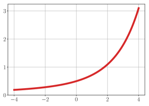
Remark 2.8.

Function $\varphi(t)=\frac{e^{t}-t-1}{t^{2}}$ used in Lemma 2.7 is convex and monotone. Its graph is shown in Figure 2.

Figure 2: Graph of function $\varphi(t)=\frac{e^{t}-t-1}{t^{2}}$.

Note that (25) are the global upper and lower second-order models of the objective (see Figure 1). It seems to be difficult to use them directly in optimization algorithms, since these models are non-convex in general. However, from Lemmas 2.5 and 2.7 we see that function $f(\cdot)$ is almost quadratic in every ball of radius $r:=1/M$. Indeed, according to (21), for any $\bm{x},\bm{y}\in\operatorname{dom}f$ s.t. $\|\bm{x}-\bm{y}\|\leq 1/M$ the Hessian is stable [26]:

$$\begin{array}[]{rcl}\frac{1}{e}\nabla^{2}f(\bm{x})&\preceq&\nabla^{2}f(\bm{y})\;\;\preceq\;\;e\nabla^{2}f(\bm{x}).\end{array}$$

Therefore, for minimizing a Quasi-Self-Concordant objective we can use a trust-region scheme with a fixed radius [26, 6], that achieves the global complexity: $\tilde{\mathcal{O}}\bigl{(}MD\bigr{)}$ iterations to solve the problem with any given accuracy (global linear rate of convergence), where $D$ is the diameter of the initial sublevel set and $\tilde{\mathcal{O}}(\cdot)$ hides logarithmic factors.

As we show in the next section, we can use instead the Gradient Regularization of Newton Method, which is easier to implement and, most importantly, it does not need to fix the value of $r=1/M$ (the trust-region radius), allowing an adaptive choice of parameter $M$.

3 Gradient Regularization of Newton Method

In this section, we propose the primal Newton scheme for minimizing Quasi-Self-Concordant objectives in the composite form (12). For a given $\bm{x}\in Q$, we consider the point $\bm{x}^{+}$ defined as

$$\boxed{\begin{array}[]{rcl}\bm{x}^{+}&\stackrel{{\scriptstyle\mathrm{def}}}{{=}}&\arg\min\limits_{\bm{y}\in Q}\Bigl{\{}\;{\langle}\nabla f(\bm{x}),\bm{y}-\bm{x}{\rangle}+\frac{1}{2}\|\bm{y}-\bm{x}\|_{\bm{x}}^{2}+\frac{\beta}{2}\|\bm{y}-\bm{x}\|^{2}+\psi(\bm{y})\;\Bigr{\}}\end{array}}$$ (26)

with regularization coefficient proportional to the current (sub)gradient norm:

$$\boxed{\begin{array}[]{rcl}\beta&:=&\sigma\|F^{\prime}(\bm{x})\|_{*}\end{array}}$$ (27)

for some $F^{\prime}(\bm{x})\in\partial F(\bm{x})$ and parameter $\sigma\geq 0$. Thus, (26) is a simple Newton step with quadratic regularization and with a possible composite component. In case $\psi\equiv 0$ (unconstrained minimization), we obtain a direct formula for one step:

$$\begin{array}[]{rcl}\bm{x}^{+}&=&\bm{x}-\Bigl{(}\nabla^{2}f(\bm{x})+\sigma\|\nabla f(\bm{x})\|_{*}\bm{B}\Bigr{)}^{-1}\nabla f(\bm{x}),\end{array}$$

which requires solving just one linear system, as in the classical Newton Method. In general, (26) is a composite quadratic minimization problem, and we can use first-order Gradient Methods [34] for solving it. Note that the objective in (26) is strongly convex for $\beta>0$, and we can expect fast linear rate of convergence for these gradient-based solvers.

Optimality condition for one step (26) is as follows (see, e.g., Theorem 3.1.23 in [34]):

$$\begin{array}[]{rcl}{\langle}\nabla f(\bm{x})+\nabla^{2}f(\bm{x})(\bm{x}^{+}-\bm{x})+\beta\bm{B}(\bm{x}^{+}-\bm{x}),\bm{y}-\bm{x}^{+}{\rangle}+\psi(\bm{y})&\geq&\psi(\bm{x}^{+}),\qquad\forall\bm{y}\in Q.\end{array}$$ (28)

Therefore, we have an access to the following special selection of the subgradient at new point:

$$\begin{array}[]{rcl}F^{\prime}(\bm{x}^{+})&\stackrel{{\scriptstyle\mathrm{def}}}{{=}}&\nabla f(\bm{x}^{+})-\nabla f(\bm{x})-\nabla^{2}f(\bm{x})(\bm{x}^{+}-\bm{x})-\beta\bm{B}(\bm{x}^{+}-\bm{x})\;\;\in\;\;\partial F(\bm{x}^{+}).\end{array}$$ (29)

Now, utilizing convexity of $\psi$, we claim the following important bound for the length of one step. This lemma is the main tool, which is used in the core of our analysis.

Lemma 3.1.

For any $F^{\prime}(\bm{x})\in\partial F(\bm{x})$, we have

$$\begin{array}[]{rcl}\|\bm{x}^{+}-\bm{x}\|&\leq&\frac{\|F^{\prime}(\bm{x})\|_{*}}{\beta+\lambda(\bm{x})},\end{array}$$ (30)

and

$$\begin{array}[]{rcl}\|\bm{x}^{+}-\bm{x}\|_{\bm{x}}^{2}&\leq&\|\bm{x}^{+}-\bm{x}\|\cdot\|F^{\prime}(\bm{x})\|_{*}\;\;\overset{\eqref{StepBound}}{\leq}\;\;\frac{\|F^{\prime}(\bm{x})\|_{*}^{2}}{\beta+\lambda(\bm{x})}.\end{array}$$ (31)

Proof.

Indeed, for $\psi^{\prime}(\bm{x}):=F^{\prime}(\bm{x})-\nabla f(\bm{x})\in\partial\psi(\bm{x})$ and $\psi^{\prime}(\bm{x}^{+}):=F^{\prime}(\bm{x}^{+})-\nabla f(\bm{x}^{+})\in\partial\psi(\bm{x}^{+})$, we obtain

$$\begin{array}[]{rcl}0&\leq&{\langle}\psi^{\prime}(\bm{x}^{+})-\psi^{\prime}(\bm{x}),\bm{x}^{+}-\bm{x}{\rangle}\;\;\overset{\eqref{FPrimeDef}}{=}\;\;{\langle}F^{\prime}(\bm{x}),\bm{x}-\bm{x}^{+}{\rangle}-\|\bm{x}^{+}-\bm{x}\|_{\bm{x}}^{2}-\beta\|\bm{x}^{+}-\bm{x}\|^{2}.\end{array}$$

Therefore, rearranging the terms and using Cauchy-Schwartz inequality, we get

$$\begin{array}[]{rcl}\|\bm{x}^{+}-\bm{x}\|\cdot\|F^{\prime}(\bm{x})\|_{*}&\geq&\beta\|\bm{x}^{+}-\bm{x}\|^{2}+\|\bm{x}^{+}-\bm{x}\|_{\bm{x}}^{2}\;\;\geq\;\;(\beta+\lambda(\bm{x}))\|\bm{x}^{+}-\bm{x}\|^{2}.\end{array}$$

which gives the required bounds. ∎

For our purposes, the most important inequality is (30). It shows that using the gradient regularization rule (27) with sufficiently big $\sigma\geq M$, we can control the multiplicative error terms in (24),(25), as follows:

$$\begin{array}[]{rcl}\varphi\bigl{(}M\|\bm{x}^{+}-\bm{x}\|\bigr{)}&\overset{\eqref{StepBound}}{\leq}&\varphi\Bigl{(}\frac{M\|F^{\prime}(\bm{x})\|^{*}}{\beta}\Bigr{)}\;\;\overset{\eqref{BetaChoice}}{=}\;\;\varphi\bigl{(}\frac{M}{\sigma}\bigr{)}\;\;\leq\;\;\varphi(1)\;\;\stackrel{{\scriptstyle\mathrm{def}}}{{=}}\;\;\rho,\end{array}$$ (32)

where we used monotonicity of $\varphi$. Note that

$$\begin{array}[]{rcl}\rho&=&e-2\;\;\approx\;\;0.718.\end{array}$$ (33)

We are ready to characterize one primal Newton step (26) with Gradient Regularization rule (27).

Theorem 3.2.

Let $\sigma\geq M$. Then, for step (26) with $\beta:=\sigma\|F^{\prime}(\bm{x})\|_{*}$ with some $F^{\prime}(\bm{x})\in\partial F(\bm{x})$, it holds

$$\begin{array}[]{rcl}{\langle}F^{\prime}(\bm{x}^{+}),\bm{x}-\bm{x}^{+}{\rangle}&\geq&\frac{1}{2\beta}\|F^{\prime}(\bm{x}^{+})\|_{*}^{2}.\end{array}$$ (34)

Proof.

From (24), we have

$$\begin{array}[]{rcl}\|F^{\prime}(\bm{x}^{+})+\beta\bm{B}(\bm{x}^{+}-\bm{x})\|_{*}&\overset{\eqref{FPrimeDef}}{=}&\|\nabla f(\bm{x}^{+})-\nabla f(\bm{x})-\nabla^{2}f(\bm{x})(\bm{x}^{+}-\bm{x})\|_{*}\\ \\ &\overset{\eqref{GradBound}}{\leq}&M\|\bm{x}^{+}-\bm{x}\|_{\bm{x}}^{2}\cdot\varphi\bigl{(}M\|\bm{x}^{+}-\bm{x}\|\bigr{)}\;\;\overset{\eqref{Rho}}{\leq}\;\;\rho M\|\bm{x}^{+}-\bm{x}\|_{\bm{x}}^{2}\\ \\ &\overset{\eqref{StepBoundX}}{\leq}&\rho M\|\bm{x}^{+}-\bm{x}\|\cdot\|F^{\prime}(\bm{x})\|_{*}\;\;\overset{\eqref{BetaChoice}}{=}\;\;\frac{\rho M}{\sigma}\beta\|\bm{x}^{+}-\bm{x}\|.\end{array}$$ (35)

Thus, taking square of both sides and rearranging the terms, we obtain

$$\begin{array}[]{rcl}{\langle}F^{\prime}(\bm{x}^{+}),\bm{x}-\bm{x}^{+}{\rangle}&\overset{\eqref{NewGradEuclidean}}{\geq}&\frac{1}{2\beta}\|F^{\prime}(\bm{x}^{+})\|_{*}^{2}\;+\;\frac{\beta}{2}\|\bm{x}^{+}-\bm{x}\|^{2}\cdot\Bigl{(}1-\bigl{[}\frac{\rho M}{\sigma}\bigr{]}^{2}\Bigr{)}\\ \\ &\geq&\frac{1}{2\beta}\|F^{\prime}(\bm{x}^{+})\|_{*}^{2},\end{array}$$

where the last bound holds due to our choice: $\sigma\geq M$. ∎

From (34), we see that one step of our method is monotone: $F(\bm{x}^{+})\leq F(\bm{x})$. Indeed, by convexity

$$\begin{array}[]{rcl}F(\bm{x})-F(\bm{x}^{+})&\geq&{\langle}F^{\prime}(\bm{x}^{+}),\bm{x}-\bm{x}^{+}{\rangle}\;\;\overset{\eqref{NewGradProgress}}{\geq}\;\;\frac{1}{2\beta}\|F^{\prime}(\bm{x}^{+})\|_{*}^{2},\end{array}$$ (36)

and for each step we have the global progress in terms of the objective function value.

Let us present our primal method in the algorithmic form.

$$\begin{array}[]{|c|}\hline\cr\\ \quad\mbox{\bf Newton Method with Gradient Regularization}\\ \\ \hline\cr\\ \begin{array}[]{l}\mbox{{\bf Choose} $\bm{x}_{0}\in Q$ and set $g_{0}=\|F^{\prime}(\bm{x}_{0})\|_{*}$ for $F^{\prime}(\bm{x}_{0})\in\partial F(\bm{x}_{0})$.}\\ \\ \mbox{\bf For $k\geq 0$ iterate:}\\[10.0pt] \mbox{1. For some $\sigma_{k}\geq 0$, compute }\\[10.0pt] $$\begin{array}[]{rcl}\bm{x}_{k+1}&=&\arg\min\limits_{\bm{y}\in Q}\Bigl{\{}{\langle}\nabla f(\bm{x}_{k}),\bm{y}-\bm{x}_{k}{\rangle}+\frac{1}{2}\|\bm{y}-\bm{x}_{k}\|_{\bm{x}_{k}}^{2}+\frac{\sigma_{k}g_{k}}{2}\|\bm{y}-\bm{x}_{k}\|^{2}+\psi(\bm{y})\Bigr{\}}.\end{array}$$\\ \\ \mbox{2. Set $g_{k+1}=\|\nabla f(\bm{x}_{k+1})-\nabla f(\bm{x}_{k})-(\nabla^{2}f(\bm{x}_{k})+\sigma_{k}g_{k}\bm{B})(\bm{x}_{k+1}-\bm{x}_{k})\|_{*}$.}\\ \\ \end{array}\\ \hline\cr\end{array}$$ (37)

Note that in this algorithm we have a freedom of choosing the regularization parameter $\sigma_{k}\geq 0$ for each iteration $k\geq 0$. A simple choice that follows directly from our theory, is the constant one:

$$\begin{array}[]{rcl}\sigma_{k}&\equiv&M,\qquad\forall k,\end{array}$$

where $M$ is the parameter of Quasi-Self-Concordance (13). However, if constant $M$ is unknown, we can do a simple adaptive search that ensures sufficient progress (36) for the objective function value. Namely, in each iteration $k\geq 0$, we choose $\sigma_{k}>0$ such that the following inequality is satisfied:

$$\begin{array}[]{rcl}{\langle}F^{\prime}(\bm{x}_{k+1}),\bm{x}_{k}-\bm{x}_{k+1}{\rangle}&\geq&\frac{g_{k+1}^{2}}{2\sigma_{k}g_{k}},\end{array}$$ (38)

by increasing $\sigma_{k}$ twice. From Theorem 3.2, we know that it will be satisfied at least for $\sigma_{k}\geq M$. Then, after accepting a certain $\sigma_{k}$ for the current iteration, we start our adaptive search in the next step from the value $\sigma_{k+1}:=\frac{\sigma_{k}}{2}$. This allows both increase and decrease of the regularization parameters. It is easy to show that the price of such adaptive search is just one extra step per iteration in average.

Note that our algorithm (37) with implementation of this adaptive procedure and using the progress condition (38) actually coincides with the recently proposed Super-Universal Newton Method (Algorithm 2 in [12] with parameter $\alpha:=1$). Therefore, our new theory also extends the analysis of the Super-Universal Newton Method [12] for the Quasi-Self-Concordant functions.

Let us justify the global linear rate for our method. For the analysis of our primal scheme, we introduce the initial sublevel set: $\mathcal{L}_{0}\stackrel{{\scriptstyle\mathrm{def}}}{{=}}\bigl{\{}\bm{x}\in Q\,:\,F(\bm{x})\leq F(\bm{x}_{0})\bigr{\}},$ and its diameter, which we assume to be bounded:

$$\begin{array}[]{rcl}D&\stackrel{{\scriptstyle\mathrm{def}}}{{=}}&\sup\limits_{\bm{x},\bm{y}\in\mathcal{L}_{0}}\|\bm{x}-\bm{y}\|\;\;<\;\;+\infty.\end{array}$$ (39)

We prove our main result.

Theorem 3.3.

Let the smooth component of problem (12) be Quasi-Self-Concordant with parameter $M\geq 0$. Let in each iteration of method (37), we choose parameter $\sigma_{k}\in[0,2M]$ such that condition (38) holds. Then, we have the global linear rate, for $k\geq 1$:

$$\begin{array}[]{rcl}F(\bm{x}_{k})-F^{\star}&\leq&\exp\Bigl{(}-\frac{k}{8MD}\Bigr{)}\bigl{(}F(\bm{x}_{0})-F^{\star}\bigr{)}\,+\,\exp\Bigl{(}-\frac{k}{4}\Bigr{)}g_{0}D.\end{array}$$ (40)

Proof.

We denote $F_{k}\stackrel{{\scriptstyle\mathrm{def}}}{{=}}F(\bm{x}_{k})-F^{\star}$. Due to convexity of $F(\cdot)$ and monotonicity of the sequence $\{F_{k}\}_{k\geq 0}$, we have

$$\begin{array}[]{rcl}F_{k}&\leq&g_{k}\|\bm{x}_{k}-\bm{x}^{\star}\|\;\;\leq\;\;g_{k}D.\end{array}$$ (41)

By concavity of logarithm, we know that

$$\begin{array}[]{rcl}\ln\frac{a}{b}&=&\ln a-\ln b\;\;\geq\;\;\frac{1}{a}(a-b),\qquad a,b>0.\end{array}$$ (42)

Then, for any $0\leq i<k$, we obtain

$$\begin{array}[]{rcl}\ln\frac{F_{i}}{F_{i+1}}&\overset{\eqref{LogConcave}}{\geq}&\frac{1}{F_{i}}(F_{i}-F_{i+1})\;\;\overset{\eqref{OneStepProgress}}{\geq}\;\;\frac{g_{i}}{2\sigma_{i}F_{i}}\cdot\bigl{[}\frac{g_{i+1}}{g_{i}}\bigr{]}^{2}\\ \\ &\overset{\eqref{FConv}}{\geq}&\frac{1}{2\sigma_{i}D}\cdot\bigl{[}\frac{g_{i+1}}{g_{i}}\bigr{]}^{2}\;\;\geq\;\;\frac{1}{4MD}\cdot\bigl{[}\frac{g_{i+1}}{g_{i}}\bigr{]}^{2}.\end{array}$$ (43)

Therefore, telescoping this bound for all iterations $0\leq i<k$ and using the inequality between arithmetic and geometric means, we get

$$\begin{array}[]{rcl}\ln\frac{F_{0}}{F_{k}}&\overset{\eqref{PreTelescopeProgress}}{\geq}&\frac{1}{4MD}\sum\limits_{i=0}^{k-1}\bigl{[}\frac{g_{i+1}}{g_{i}}\bigr{]}^{2}\;\;\geq\;\;\frac{k}{4MD}\biggl{[}\,\prod\limits_{i=0}^{k-1}\frac{g_{i+1}}{g_{i}}\,\biggr{]}^{2/k}\;\;=\;\;\frac{k}{4MD}\bigl{[}\frac{g_{k}}{g_{0}}\bigr{]}^{2/k}\\ \\ &=&\frac{k}{4MD}\exp\Bigl{[}\frac{2}{k}\ln\frac{g_{k}}{g_{0}}\Bigr{]}\;\;\geq\;\;\frac{k}{4MD}\Bigl{(}1+\frac{2}{k}\ln\frac{g_{k}}{g_{0}}\Bigr{)}\;\;\overset{\eqref{FConv}}{\geq}\;\;\frac{k}{4MD}\Bigl{(}1+\frac{2}{k}\ln\frac{F_{k}}{g_{0}D}\Bigr{)}.\end{array}$$ (44)

Let us consider two cases.

1. We have $\frac{2}{k}\ln\frac{F_{k}}{g_{0}D}\leq-\frac{1}{2}\;\;\Leftrightarrow\;\;F_{k}\leq\exp(-k/4)g_{0}D$.

2. Otherwise, $\frac{2}{k}\ln\frac{F_{k}}{g_{0}D}\geq-\frac{1}{2}$, substituting which into (44) gives

   $$\begin{array}[]{rcl}\ln\frac{F_{0}}{F_{k}}&\geq&\frac{k}{8MD}\quad\Leftrightarrow\quad F_{k}\;\;\leq\;\;\exp\Bigl{(}-\frac{k}{8MD}\Bigr{)}F_{0}.\end{array}$$

Combining these two cases, we obtain (40). ∎

Since our problem class is scale-invariant, it is a natural goal to ensure the relative accuracy guarantee. Thus, we are interested to find a point $\bm{x}_{k}$ such that

$$\begin{array}[]{rcl}F(\bm{x}_{k})-F^{\star}&\leq&\varepsilon\cdot\bigl{(}F(\bm{x}_{0})-F^{\star}\bigr{)},\end{array}$$ (45)

for a certain desired $0<\varepsilon<1$. Note that (45) can be easily translated into absolute accuracy for a given tolerance level $\varepsilon^{\prime}$ by setting $\varepsilon:=\frac{\varepsilon^{\prime}}{F(\bm{x}_{0})-F^{\star}}$. At the same time, our accuracy parameter $\varepsilon$ in (45) does not depend on any particular scaling of the objective function, which can be arbitrary in practice. Then, directly from Theorem 3.3, we obtain the following global complexity guarantee.

Corollary 3.4.

The number of iterations of method (37) to reach $\varepsilon$-accuracy is bounded as

$$\begin{array}[]{rcl}k&\leq&\mathcal{O}\Bigl{(}MD\ln\frac{1}{\varepsilon}+\ln\frac{Dg_{0}}{\varepsilon(F(\bm{x}_{0})-F^{\star})}\Bigr{)}.\end{array}$$ (46)

We see that the main complexity factor for solving problem (12) with a Quasi-Self-Concordant objective is the following condition number $\kappa\;\stackrel{{\scriptstyle\mathrm{def}}}{{=}}\;MD$. Note that this is the same complexity as we can prove for the trust-region scheme on Hessian-stable functions (see the discussion in the end of previous section). However, our method is much easier to implement, using only the basic steps of the form (2). Moreover, our algorithm admits using a simple adaptive search, which does not need to know the actual value of parameter $M$.

In Sections 5 and 6, we show how to improve this factor with the Dual and Accelerated Newton schemes. The latter method achieves the accelerated complexity $\tilde{\mathcal{O}}(\kappa^{2/3})$. The key to our analysis is the local behaviour of our primal Newton method (37), which we study in the next section.

4 Local Quadratic Convergence

Let us assume that $\lambda(\bm{x}_{0})>0$. Then, we have $\lambda(\bm{x})>0$ for all $\bm{x}\in\operatorname{dom}f$ (see Remark 2.6). It is convenient to consider the following scale-invariant measure of convergence:

$$\begin{array}[]{rcl}\eta(\bm{x})&\stackrel{{\scriptstyle\mathrm{def}}}{{=}}&\frac{\|F^{\prime}(\bm{x})\|_{*}}{\lambda(\bm{x})},\qquad\bm{x}\in Q,\end{array}$$

for a given particular selection of subgradients $F^{\prime}(\bm{x})\in\partial F(\bm{x})$. We also introduce the following local region, for some $0<c\leq 1$:

$$\begin{array}[]{rcl}\mathcal{G}_{c}&\stackrel{{\scriptstyle\mathrm{def}}}{{=}}&\Bigl{\{}\bm{x}\in Q\;:\;\eta(\bm{x})\leq\frac{c}{M}\Bigr{\}}.\end{array}$$ (47)

Then, for one primal step $\bm{x}\mapsto\bm{x}^{+}$ of our method (26) from $\bm{x}\in\mathcal{G}_{c}$, and using the Gradient Regularization $\beta=\sigma\|F^{\prime}(\bm{x})\|_{*}$ with an arbitrary $\sigma\geq 0$, we get

$$\begin{array}[]{rcl}\|F^{\prime}(\bm{x}^{+})\|_{*}&\overset{\eqref{FPrimeDef},\eqref{GradBound}}{\leq}&M\|\bm{x}^{+}-\bm{x}\|_{\bm{x}}^{2}\cdot\varphi(M\|\bm{x}^{+}-\bm{x}\|)+\beta\|\bm{x}^{+}-\bm{x}\|\\ \\ &\overset{\eqref{StepBound},\eqref{StepBoundX}}{\leq}&\frac{M\|F^{\prime}(\bm{x})\|^{2}_{*}}{\lambda(\bm{x})}\cdot\varphi(M\eta(\bm{x}))+\frac{\sigma\|F^{\prime}(\bm{x})\|_{*}^{2}}{\lambda(\bm{x})}\;\;\overset{\eqref{LocalRegion}}{\leq}\;\;\frac{\|F^{\prime}(\bm{x})\|_{*}^{2}}{\lambda(\bm{x})}\cdot(\rho M+\sigma),\end{array}$$ (48)

where $\rho\stackrel{{\scriptstyle\mathrm{def}}}{{=}}\varphi(1)$ is an absolute constant (33). Dividing the left hand side of (48) by $\lambda(\bm{x}^{+})$, we obtain

$$\begin{array}[]{rcl}\eta(\bm{x}^{+})&\overset{\eqref{HessBound}}{\leq}&\frac{\|F^{\prime}(\bm{x}^{+})\|_{*}}{\lambda(\bm{x})}\cdot e^{M\|\bm{x}^{+}-\bm{x}\|}\;\;\overset{\eqref{StepBound}}{\leq}\;\;\frac{\|F^{\prime}(\bm{x}^{+})\|_{*}}{\lambda(\bm{x})}\cdot e^{M\eta(\bm{x})}\\ \\ &\overset{\eqref{LocalRegion}}{\leq}&\frac{\|F^{\prime}(\bm{x}^{+})\|_{*}}{\lambda(\bm{x})}\cdot e\;\;\overset{\eqref{LocalStep}}{\leq}\;\;\eta(\bm{x})^{2}\cdot e(\rho M+\sigma),\end{array}$$ (49)

which is the quadratic convergence in terms of our measure $\eta(\bm{x})$. Thus, we established the following.

Theorem 4.1.

Let the smooth component of problem (12) be Quasi-Self-Concordant with parameter $M>0$. Consider the iterations $\{\bm{x}_{k}\}_{k\geq 0}$ of method (37) with any $\sigma_{k}\in[0,2M]$, and assume that $\bm{x}_{0}\in\mathcal{G}_{1/18}$. Then, we have the quadratic rate, for $k\geq 0$:

$$\begin{array}[]{rcl}\eta(\bm{x}_{k})&\leq&\frac{1}{9M}\cdot\bigl{(}\frac{1}{2}\bigr{)}^{2^{k}}.\end{array}$$ (50)

Proof.

Indeed, for any $k\geq 1$, we have $\eta(\bm{x}_{k})\overset{\eqref{LocalMeasureStep}}{\leq}\eta(\bm{x}_{k-1})^{2}\cdot e(\rho M+\sigma)\leq\eta(\bm{x}_{k-1})^{2}\cdot 9M$. Therefore, by induction $\bm{x}_{k}\in\mathcal{G}_{1/18}$ for all $k\geq 0$, and we get

$$\begin{array}[]{rcl}(\eta(\bm{x}_{k})\cdot 9M)&\leq&(\eta(\bm{x}_{k-1})\cdot 9M)^{2}\;\;\leq\;\;\ldots\;\;\leq\;\;(\eta(\bm{x}_{0})\cdot 9M)^{2^{k}}.\end{array}$$

Taking into account that $\bm{x}_{0}\in\mathcal{G}_{1/18}$ finishes the proof. ∎

We see that for achieving the local quadratic convergence (50), we can perform just pure Newton steps ($\sigma_{k}\equiv 0$).

Let us consider a particular consequence of our theory for minimizing strongly convex functions, that will be useful in the next section for constructing the Dual Newton Method. Thus, we assume that the Hessian is uniformly bounded from below, for some $\mu>0$:

$$\begin{array}[]{rcl}\lambda(\bm{x})&\geq&\mu,\qquad\forall\bm{x}\in Q,\end{array}$$ (51)

and consider one primal pure Newton step (26) $\bm{x}\mapsto\bm{x}^{+}$ with $\sigma:=0$ (no regularization). Then, assuming that point $\bm{x}$ belongs to the following local region, for some selection of the subgradients:

$$\begin{array}[]{rcl}\mathcal{U}&\stackrel{{\scriptstyle\mathrm{def}}}{{=}}&\Bigl{\{}\bm{x}\in Q\;:\;\|F^{\prime}(\bm{x})\|_{*}\leq\frac{\mu}{2M}\Bigr{\}},\end{array}$$ (52)

we get

$$\begin{array}[]{rcl}\|F^{\prime}(\bm{x}^{+})\|_{*}&\overset{\eqref{FPrimeDef},\eqref{GradBound}}{\leq}&M\|\bm{x}^{+}-\bm{x}\|_{\bm{x}}^{2}\cdot\varphi(M\|\bm{x}^{+}-\bm{x}\|)\\ \\ &\overset{\eqref{StepBound},\eqref{StepBoundX},\eqref{StronglyConvex}}{\leq}&\frac{M\|F^{\prime}(\bm{x})\|_{*}^{2}}{\mu}\cdot\varphi\Bigl{(}\frac{M\|F^{\prime}(\bm{x})\|_{*}}{\mu}\Bigr{)}\;\;\overset{\eqref{Local2}}{\leq}\;\;\frac{M\|F^{\prime}(\bm{x})\|_{*}^{2}}{\mu}\cdot\varphi(1/2).\end{array}$$ (53)

Thus, we can justify the following quadratic convergence for our specific case.

Theorem 4.2.

Let the smooth component of problem (12) be Quasi-Self-Concordant with parameter $M>0$ and strongly convex with parameter $\mu>0$. Consider the iterations of the pure Newton Method:

$$\begin{array}[]{rcl}\bm{x}_{k+1}&=&\arg\min\limits_{\bm{y}\in Q}\Bigl{\{}{\langle}\nabla f(\bm{x}_{k}),\bm{y}-\bm{x}_{k}{\rangle}+\frac{1}{2}\|\bm{y}-\bm{x}_{k}\|_{\bm{x}_{k}}^{2}+\psi(\bm{y})\Bigr{\}},\qquad k\geq 0,\end{array}$$

and assume that $\bm{x}_{0}\in\mathcal{U}$. Then, we have the quadratic rate, for $k\geq 0$:

$$\begin{array}[]{rcl}\|F^{\prime}(\bm{x}_{k})\|_{*}&\leq&\frac{\mu}{2M}\cdot\bigl{(}\frac{1}{e}\bigr{)}^{2^{k}}.\end{array}$$ (54)

Proof.

Indeed, for any $k\geq 1$, we have

$$\begin{array}[]{rcl}\frac{M\varphi(1/2)}{\mu}\|F^{\prime}(\bm{x}_{k})\|_{*}&\overset{\eqref{LocalStep2}}{\leq}&\Bigl{(}\frac{M\varphi(1/2)}{\mu}\|F^{\prime}(\bm{x}_{k-1})\|_{*}\Bigr{)}^{2}\;\;\leq\;\;\ldots\;\;\leq\;\;\Bigl{(}\frac{M\varphi(1/2)}{\mu}\|F^{\prime}(\bm{x}_{0})\|_{*}\Bigr{)}^{2^{k}}.\end{array}$$

It remains to notice that $1/2\leq\varphi(1/2)\leq 2/e$. Using that $\bm{x}_{0}\in\mathcal{U}$ completes the proof. ∎

5 Dual Newton Method

In this section, we discover another possibility for minimizing our objective (12) which is based on inexact proximal-point iterations [31, 28, 42, 44, 43]. Thus, at each iteration $k\geq 0$, we minimize the following augmented function:

$$\begin{array}[]{rcl}h_{k}(\bm{x})&:=&F(\bm{x})+\frac{1}{2a_{k+1}}\|\bm{x}-\bm{x}_{k}\|^{2},\end{array}$$ (55)

where $\bm{x}_{k}$ is the current point and $a_{k+1}>0$ is some regularization constant. Note that the smooth component of (55) is Quasi-Self-Concordant with parameter $M$ and strongly convex with constant $\mu=\frac{1}{a_{k+1}}$. Hence, choosing

$$\boxed{\begin{array}[]{rcl}a_{k+1}&:=&\frac{1}{2M\|F^{\prime}(\bm{x}_{k})\|_{*}}\end{array}}$$

we ensure that point $\bm{x}_{k}$ is in the local region of quadratic convergence (52) of the Newton Method, and we can minimize objective (55) very fast up to any desirable precision, to obtain the next iterate $\bm{x}_{k+1}\approx\arg\min\limits_{\bm{x}}h_{k}(\bm{x})$. This approach resembles the standard Path-Following scheme for minimizing the classic Self-Concordant functions [34]. It was also explored recently in [14] as an application of high-order Tensor Methods.

$$\begin{array}[]{|c|}\hline\cr\\ \quad\mbox{\bf Dual Newton Method $\mathscr{D}(f,\psi,\bm{x}_{0},M,\nu)$}\\ \\ \hline\cr\\ \begin{array}[]{l}\mbox{{Initialize} $g_{0}=\|F^{\prime}(\bm{x}_{0})\|_{*}$ for $F^{\prime}(\bm{x}_{0})\in\partial F(\bm{x}_{0})$.}\\[10.0pt] \mbox{\bf For $k\geq 0$ iterate:}\\[10.0pt] \mbox{1. Set $\bm{z}_{0}=\bm{x}_{k}$.}\\[10.0pt] \mbox{2. {For $t\geq 0$ iterate:}}\\[10.0pt] \mbox{$\quad\;$2-a. Compute}\\[5.0pt] $$\begin{array}[]{rcl}\qquad\bm{z}_{t+1}&=&\arg\min\limits_{\bm{y}\in Q}\Bigl{\{}{\langle}\nabla f(\bm{z}_{t}),\bm{y}-\bm{z}_{t}{\rangle}+\frac{1}{2}\|\bm{y}-\bm{z}_{t}\|_{\bm{z}_{t}}^{2}+Mg_{k}\|\bm{y}-\bm{x}_{k}\|^{2}+\psi(\bm{y})\Bigr{\}}.\end{array}$$\\[10.0pt] \mbox{$\quad\;$2-b. Set $\bm{s}_{t+1}=\nabla f(\bm{z}_{t+1})-\nabla f(\bm{z}_{t})-\nabla^{2}f(\bm{z}_{t})(\bm{z}_{t+1}-\bm{z}_{t}).$ }\\[10.0pt] \mbox{$\quad\;${Until $\|\bm{s}_{t+1}\|_{*}\leq\frac{2Mg_{k}\nu}{(k+1)^{2}}.$}}\\[10.0pt] \mbox{3. Set $\bm{x}_{k+1}=\bm{z}_{t+1}$ and $g_{k+1}=\|\bm{s}_{t+1}-2Mg_{k}B(\bm{x}_{k+1}-\bm{x}_{k})\|_{*}$.}\\[10.0pt] \mbox{4. If $g_{k+1}\leq\nu$ then {return} $\bm{x}_{k+1}$.}\\ \\ \end{array}\\ \hline\cr\end{array}$$ (56)

In this algorithm, we need to pass the parameter of Quasi-Self-Concordance $M$ for the smooth component of the objective. The method returns a point $\bar{\bm{x}}\in Q$ with a desired bound for the (sub)gradient norm: $\|F^{\prime}(\bar{\bm{x}})\|_{*}\leq\nu$, where $\nu>0$ is a given tolerance.

Note that the first iteration $\bm{z}_{0}\mapsto\bm{z}_{1}$ of the inner loop in (56) is equivalent to one step of the primal method. However, we do several iterations of the inner loop until we find a good minimizer of the augmented objective, that has a small gradient norm: $\|h^{\prime}(\bm{x}_{k+1})\|_{*}\leq\frac{2Mg_{k}\nu}{(k+1)^{2}}.$

It appears that the resulting Dual Newton Method is very suitable for minimizing the dual objects (the gradients) and importantly it provides us with a hot-start possibility, which we use extensively for building our accelerated method in the next section. We establish the following global guarantee.

Lemma 5.1.

For the iterations of method (56), we have

$$\begin{array}[]{rcl}\sum\limits_{i=1}^{k}a_{i}\bigl{(}F(\bm{x}_{i})-F^{\star}\bigr{)}+\frac{1}{2}\sum\limits_{i=1}^{k}a_{i}^{2}\|F^{\prime}(\bm{x}_{i})\|_{*}^{2}&\leq&\frac{1}{2}(\|\bm{x}_{0}-\bm{x}^{\star}\|+2\nu)^{2},\qquad k\geq 1.\end{array}$$ (57)

Proof.

Let us prove by induction the following bound, for all $k\geq 0$:

$$\begin{array}[]{rcl}\frac{1}{2}\|\bm{x}_{0}-\bm{x}^{\star}\|^{2}+\sum\limits_{i=1}^{k}a_{i}F^{\star}+C_{k}&\geq&\frac{1}{2}\|\bm{x}_{k}-\bm{x}^{\star}\|^{2}+\sum\limits_{i=1}^{k}a_{i}F(\bm{x}_{i})+\frac{1}{2}\sum\limits_{i=1}^{k}a_{i}^{2}\|F^{\prime}(\bm{x}_{i})\|_{*}^{2},\end{array}$$ (58)

where

$$\begin{array}[]{rcl}C_{k}&\stackrel{{\scriptstyle\mathrm{def}}}{{=}}&\frac{1}{2}\sum\limits_{i=1}^{k}\xi_{i}^{2}+\sum\limits_{i=1}^{k}\xi_{i}\|\bm{x}_{i-1}-x^{\star}\|,\qquad\xi_{i}\;\;\stackrel{{\scriptstyle\mathrm{def}}}{{=}}\;\;\frac{\eta}{i^{2}}.\end{array}$$

Inequality (58) obviously holds for $k=0$. Assume that it holds for some $k\geq 0$ and consider one iterations of the method. We have

$$\begin{array}[]{cl}&\frac{1}{2}\|\bm{x}_{0}-\bm{x}^{\star}\|^{2}+\sum\limits_{i=1}^{k+1}a_{i}F^{\star}\\[10.0pt] &\overset{\eqref{DualInduct}}{\geq}\;\;\frac{1}{2}\|\bm{x}_{k}-\bm{x}^{\star}\|^{2}+a_{k+1}F^{\star}+\sum\limits_{i=1}^{k}a_{i}F(\bm{x}_{i})+\frac{1}{2}\sum\limits_{i=1}^{k}a_{i}^{2}\|F^{\prime}(\bm{x}_{i})\|_{*}^{2}-C_{k}.\end{array}$$ (59)

Note that the stopping condition for the inner loop in Step 2-c ensures that

$$\begin{array}[]{rcl}\frac{\xi_{k+1}}{a_{k+1}}&\geq&\|\bm{s}_{t+1}\|_{*}\;\;=\;\;\|F^{\prime}(\bm{x}_{k+1})+\frac{1}{a_{k+1}}B(\bm{x}_{k+1}-\bm{x}_{k})\|_{*}.\end{array}$$ (60)

Taking square of both sides of (60) and rearranging the terms, we obtain

$$\begin{array}[]{rcl}a_{k+1}{\langle}F^{\prime}(\bm{x}_{k+1}),\bm{x}_{k}-\bm{x}_{k+1}{\rangle}&\geq&\frac{a_{k+1}^{2}}{2}\|F^{\prime}(\bm{x}_{k+1})\|_{*}^{2}+\frac{1}{2}\|\bm{x}_{k}-\bm{x}_{k+1}\|^{2}-\frac{1}{2}\xi_{k+1}^{2}\end{array}$$ (61)

Therefore, we can estimate the first two terms in the right hand side of (59), as follows

$$\begin{array}[]{cl}&\frac{1}{2}\|\bm{x}_{k}-\bm{x}^{\star}\|^{2}+a_{k+1}F^{\star}\;\;\geq\;\;\frac{1}{2}\|\bm{x}_{k}-\bm{x}^{\star}\|^{2}+a_{k+1}\bigl{[}F(\bm{x}_{k+1})+{\langle}F^{\prime}(\bm{x}_{k+1}),\bm{x}^{\star}-\bm{x}_{k+1}{\rangle}\bigr{]}\\[10.0pt] &\;=\;\,\frac{1}{2}\|\bm{x}_{k+1}-\bm{x}^{\star}\|^{2}+a_{k+1}F(\bm{x}_{k+1})+a_{k+1}{\langle}F^{\prime}(\bm{x}_{k+1}),\bm{x}_{k}-\bm{x}_{k+1}{\rangle}\\[10.0pt] &\qquad\qquad+\;\frac{1}{2}\|\bm{x}_{k}-\bm{x}_{k+1}\|^{2}+{\langle}B(\bm{x}_{k}-\bm{x}_{k+1}),\bm{x}_{k+1}-\bm{x}^{\star}{\rangle}+a_{k+1}{\langle}F^{\prime}(\bm{x}_{k+1}),\bm{x}^{\star}-\bm{x}_{k}{\rangle}\\[10.0pt] &\overset{\eqref{DualStepProgress}}{\geq}\;\frac{1}{2}\|\bm{x}_{k+1}-\bm{x}^{\star}\|^{2}+a_{k+1}F(\bm{x}_{k+1})+\frac{a_{k+1}^{2}}{2}\|F^{\prime}(\bm{x}_{k+1})\|_{*}^{2}-\frac{1}{2}\xi_{k+1}^{2}\\[10.0pt] &\qquad\qquad+\;{\langle}a_{k+1}F^{\prime}(\bm{x}_{k+1})+B(\bm{x}_{k+1}-\bm{x}_{k}),\bm{x}^{\star}-\bm{x}_{k}{\rangle}\\[10.0pt] &\overset{\eqref{DualDeltaBound}}{\geq}\;\frac{1}{2}\|\bm{x}_{k+1}-\bm{x}^{\star}\|^{2}+a_{k+1}F(\bm{x}_{k+1})+\frac{a_{k+1}^{2}}{2}\|F^{\prime}(\bm{x}_{k+1})\|_{*}^{2}-\frac{1}{2}\xi_{k+1}^{2}-\xi_{k}\|\bm{x}_{k}-\bm{x}^{\star}\|.\end{array}$$

Combining it with (59), we obtain (58) for the next iterate. Thus, (58) is proven for all $k\geq 0$.

Now, let us denote $R_{k}\stackrel{{\scriptstyle\mathrm{def}}}{{=}}\|\bm{x}_{0}-\bm{x}^{\star}\|+\sum_{i=1}^{k}\xi_{i}$, and prove by induction that

$$\begin{array}[]{rcl}\frac{1}{2}\|\bm{x}_{0}-\bm{x}^{\star}\|^{2}+C_{k}&\leq&\frac{1}{2}R_{k}^{2},\end{array}$$ (62)

which trivially holds for $k=0$. Assume that (62) holds for some $k\geq 0$. Then, from (58) we have

$$\begin{array}[]{rcl}\|\bm{x}_{k}-\bm{x}^{\star}\|&\leq&R_{k},\end{array}$$ (63)

and

$$\begin{array}[]{rcl}\frac{1}{2}\|\bm{x}_{0}-\bm{x}^{\star}\|^{2}+C_{k+1}&=&\frac{1}{2}\|\bm{x}_{0}-\bm{x}^{\star}\|^{2}+C_{k}+\frac{1}{2}\xi_{k+1}^{2}+\xi_{k+1}\|\bm{x}_{k}-\bm{x}^{\star}\|\\[10.0pt] &\overset{\eqref{DualRBound},\eqref{DualRkBound}}{\leq}&\frac{1}{2}R_{k}^{2}+\frac{1}{2}\xi_{k+1}^{2}+\xi_{k+1}R_{k}\;\;=\;\;\frac{1}{2}(R_{k}+\xi_{k+1})^{2}\;\;=\;\;\frac{1}{2}R_{k+1}^{2},\end{array}$$

which proves (62) for all $k\geq 0$. Thus, we justified that

$$\begin{array}[]{rcl}\sum\limits_{i=1}^{k}a_{i+1}(F(\bm{x}_{i})-F^{\star})+\frac{1}{2}\sum\limits_{i=1}^{k}a_{i}^{2}\|F^{\prime}(\bm{x}_{i})\|^{2}&\overset{\eqref{DualInduct},\eqref{DualRBound}}{\leq}&\frac{1}{2}R_{k}^{2}.\end{array}$$

It remains to notice that $R_{k}\leq\|\bm{x}_{0}-\bm{x}^{\star}\|+2\nu$, $\forall k\geq 0$. ∎

From inequality (57), we see that the method has a convergence both in terms of the functional residual and in terms of the gradient norm. We prove the following theorem.

Theorem 5.2.

Let the smooth component of problem (12) be Quasi-Self-Concordant with parameter $M>0$. Then, for the iterations of method (56) with tolerance $\nu>0$, we have the global linear rate:

$$\begin{array}[]{rcl}\|F^{\prime}(\bm{x}_{k})\|_{*}&\leq&\exp\Bigl{(}2M^{2}(\|\bm{x}_{0}-\bm{x}^{\star}\|+2\nu)^{2}-\frac{k}{2}\Bigr{)}\|F^{\prime}(\bm{x}_{0})\|_{*},\qquad k\geq 1.\end{array}$$ (64)

Moreover, during the first $k$ iterations of the method, the total number $N_{k}$ of second-order oracle calls is bounded as

$$\begin{array}[]{rcl}N_{k}&\leq&k\cdot\Bigl{(}1+\frac{1}{\ln 2}\ln\ln\frac{(k+1)^{2}}{2M\nu}\Bigr{)}.\end{array}$$ (65)

Proof.

Estimate (64) follows immediately from (57) and our choice of parameter $a_{k+1}=\frac{1}{2M\|F^{\prime}(\bm{x}_{k})\|_{*}}$. Indeed, using the inequality between arithmetic and geometric means, we get

$$\begin{array}[]{rcl}\frac{1}{2}(\|\bm{x}_{0}-\bm{x}^{\star}\|+2\nu)^{2}&\overset{\eqref{DualNewtonGuarantee}}{\geq}&\frac{1}{8M^{2}}\sum\limits_{i=1}^{k}\frac{\|F^{\prime}(\bm{x}_{i})\|_{*}^{2}}{\|F^{\prime}(\bm{x}_{i-1})\|_{*}^{2}}\;\;\geq\;\;\frac{k}{8M^{2}}\biggl{[}\prod\limits_{i=1}^{k}\frac{\|F^{\prime}(\bm{x}_{i})\|_{*}}{\|F^{\prime}(\bm{x}_{i-1})\|_{*}}\biggr{]}^{2/k}\\ \\ &=&\frac{k}{8M^{2}}\Bigl{[}\frac{\|F^{\prime}(\bm{x}_{k})\|_{*}}{\|F^{\prime}(\bm{x}_{0})\|_{*}}\Bigr{]}^{2/k}\;\;=\;\;\frac{k}{8M^{2}}\exp\Bigl{[}\frac{2}{k}\ln\frac{\|F^{\prime}(\bm{x}_{k})\|_{*}}{\|F^{\prime}(\bm{x}_{0})\|_{*}}\Bigr{]}\\ \\ &\geq&\frac{k}{8M^{2}}\Bigl{(}1+\frac{2}{k}\ln\frac{\|F^{\prime}(\bm{x}_{k})\|_{*}}{\|F^{\prime}(\bm{x}_{0})\|_{*}}\Bigr{)}\;\;=\;\;\frac{k}{8M^{2}}+\frac{1}{4M^{2}}\ln\frac{\|F^{\prime}(\bm{x}_{k})\|_{*}}{\|F^{\prime}(\bm{x}_{0})\|_{*}},\end{array}$$

which is (64).

For iteration $i\geq 0$, let us denote by $t_{i}\geq 1$ the corresponding number of second-order oracle calls (executions of Step 2-a of the method). Then, due to the local quadratic convergence (Theorem 4.2), it is enough to ensure

$$\begin{array}[]{rcl}\frac{\mu}{2M}\cdot\bigl{(}\frac{1}{e}\bigr{)}^{2^{t_{i}}}\;\;=\;\;\frac{1}{2Ma_{k+1}}\cdot\bigl{(}\frac{1}{e}\bigr{)}^{2^{t_{i}}}&\leq&\delta_{i+1}\;\;=\;\;\frac{\nu}{(i+1)^{2}a_{i+1}},\end{array}$$

which is satisfied for $t_{i}\geq\frac{1}{\ln 2}\ln\ln\frac{(i+1)^{2}}{\nu}$. Therefore, the total number of second-order oracle calls $N_{k}$ during the first $k$ iterations is bounded as

$$\begin{array}[]{rcl}N_{k}&=&\sum\limits_{i=1}^{k}t_{i}\;\;\leq\;\;\sum\limits_{i=1}^{k}\Bigl{(}1+\frac{1}{\ln 2}\ln\ln\frac{(i+1)^{2}}{\nu}\Bigr{)}\;\;\leq\;\;k\cdot\Bigl{(}1+\frac{1}{\ln 2}\ln\ln\frac{(k+1)^{2}}{\nu}\Bigr{)},\end{array}$$

which completes the proof. ∎

Corollary 5.3.

The number of iterations of method (56) to reach $\|F^{\prime}(\bm{x}_{k})\|_{*}\leq\nu$ is bounded as

$$\begin{array}[]{rcl}k&\leq&\mathcal{O}\Bigl{(}(M\|\bm{x}_{0}-\bm{x}^{\star}\|)^{2}+(M\nu)^{2}+\ln\frac{\|F^{\prime}(\bm{x}_{0})\|_{*}}{\nu}\Bigr{)}.\end{array}$$ (66)

It is important that we obtained explicit distance from the initial point to the solution $\|\bm{x}_{0}-\bm{x}^{\star}\|$ in the right hand side of (66), as opposed to the primal method, where we had the diameter of the initial sublevel set $D$ (see (46)). Although, we have square of the condition number $\kappa^{2}$ in (66), the hot-start possibility will be very useful for us to build the accelerated scheme in the next section, which achieves the improved complexity factor $\kappa^{2/3}$.

A similar observation was also made in [27] (for different high-order methods), where the presence of the explicit distance to the solution helped to prove the optimal accelerated complexity.

6 Accelerated Newton Scheme

Let us present our accelerated second-order scheme, which is based on contracting proximal-point iterations [13]. In our algorithm, we have two sequences of points: $\{\bm{x}_{k}\}_{k\geq 0}$ (the main sequence), and $\{\bm{v}_{k}\}_{k\geq 0}$ (the proximal sequence). Let us fix a contraction parameter $\gamma\in(0,1)$ and the following sequences, for $k\geq 1$:

$$\begin{array}[]{rcl}A_{k}&:=&A_{0}(1-\gamma)^{-k}\;\;\geq\;\;A_{0}e^{k\gamma},\qquad\text{and}\qquad a_{k}\;\;:=\;\;A_{k}-A_{k-1}\;\;=\;\;\frac{\gamma}{1-\gamma}A_{k-1},\end{array}$$ (67)

where $A_{0}>0$ is some initial constant. Hence, we have $\frac{a_{k}}{A_{k}}\equiv\gamma$, $\forall k\geq 1$. The exponential grows of $A_{k}$ will determine the convergence rate of our method.

At iteration $k\geq 1$ of our accelerated scheme, we minimize the following augmented objective with contracted smooth part (compare with (55)):

$$\begin{array}[]{rcl}h_{k}(\bm{x})&:=&\underbrace{\textstyle A_{k+1}f\bigl{(}\gamma\bm{x}+(1-\gamma)\bm{x}_{k}\bigr{)}}_{\stackrel{{\scriptstyle\mathrm{def}}}{{=}}\;\ \bar{f_{k}}(\bm{x})}\;+\;\underbrace{\textstyle a_{k+1}\psi(\bm{x})+\frac{1}{2}\|\bm{x}-\bm{v}_{k}\|^{2}}_{\stackrel{{\scriptstyle\mathrm{def}}}{{=}}\;\bar{\psi}_{k}(\bm{x})}.\end{array}$$ (68)

Even though this objective is strongly convex, it is difficult to control the region of its local quadratic convergence due the contraction of the smooth part. Instead, for minimizing (68), we apply already developed Dual Newton Method (56) from the previous section as the inner procedure.

Note that the smooth part $\bar{f}_{k}(\cdot)$ of (68) is Quasi-Self-Concordant with parameter $\gamma M$. Let us denote by $\bm{v}_{k+1}^{\star}\stackrel{{\scriptstyle\mathrm{def}}}{{=}}\arg\min_{\bm{x}}h_{k}(\bm{x})$ its exact minimum, and $\bm{v}_{k+1}\approx\bm{v}_{k+1}^{\star}$ is a point that we employ in our scheme, with the following guarantee, for some tolerance parameter $\nu_{k+1}>0$:

$$\begin{array}[]{rcl}\|h_{k}^{\prime}(\bm{v}_{k+1})\|_{*}&\leq&\nu_{k+1}.\end{array}$$ (69)

Since the function $h_{k}(\cdot)$ is $1$-strongly convex, we have

$$\begin{array}[]{rcl}\|\bm{v}_{k+1}-\bm{v}_{k+1}^{\star}\|^{2}&\leq&{\langle}h_{k}^{\prime}(\bm{v}_{k+1}),\bm{v}_{k+1}-\bm{v}_{k+1}^{\star}{\rangle}\;\;\overset{\eqref{InexactVk1}}{\leq}\;\;\nu_{k+1}\|\bm{v}_{k+1}-\bm{v}_{k+1}^{\star}\|.\end{array}$$

Thus, $\|\bm{v}_{k+1}-\bm{v}_{k+1}^{\star}\|\leq\nu_{k+1}$ and

$$\begin{array}[]{rcl}\|\bm{v}_{k}-\bm{v}_{k+1}^{\star}\|&\leq&\|\bm{v}_{k}-\bm{v}_{k+1}\|+\nu_{k+1}.\end{array}$$ (70)

Therefore, minimizing (68) by the Dual Newton Method and using $\bm{v}_{k}$ as the initial point,

$$\boxed{\begin{array}[]{rcl}\bm{v}_{k+1}&:=&\mathscr{D}(\bar{f}_{k},\bar{\psi}_{k},\bm{v}_{k},\gamma M,\nu_{k+1}),\end{array}}$$

we reach guarantee (69) with the following number of iteration of our inner method:

$$\begin{array}[]{rcl}I_{k}&\overset{\eqref{DualNewtonComplexity}}{\leq}&\mathcal{O}\Bigl{(}\gamma^{2}M^{2}\|\bm{v}_{k}-\bm{v}_{k+1}\|^{2}+\gamma^{2}M^{2}\nu_{k+1}^{2}+\ln\frac{\|h^{\prime}(\bm{v}_{k})\|_{*}}{\nu_{k+1}}\Bigr{)},\end{array}$$ (71)

which we are able to effectively control. Thus, we come to our accelerated method.

$$\begin{array}[]{|c|}\hline\cr\\ \quad\mbox{\bf Accelerated Newton Scheme}\\ \\ \hline\cr\\ \begin{array}[]{l}\mbox{{\bf Choose} $\bm{x}_{0}\in Q$, $R>0$, $A_{0}>0$, and $\gamma\in(0,1)$. Set $\bm{v}_{0}=\bm{x}_{0}$.}\\ \\ \mbox{\bf For $k\geq 0$ iterate:}\\[10.0pt] \mbox{1. Set $A_{k+1}=\frac{1}{1-\gamma}A_{k}$, $a_{k+1}=\frac{\gamma}{1-\gamma}A_{k}$, and $\nu_{k+1}=\frac{R}{(k+1)^{2}}$.}\\ \\ \mbox{2. Set up contracted smooth part }\\[10.0pt] $$\begin{array}[]{rcl}\qquad\qquad\bar{f}_{k}(\bm{x})&=&A_{k+1}f\bigl{(}\gamma\bm{x}+(1-\gamma)\bm{x}_{k}\bigr{)}\end{array}$$\\[10.0pt] \mbox{ and augmented composite part }\\[10.0pt] $$\begin{array}[]{rcl}\qquad\qquad\bar{\psi}_{k}(\bm{x})&=&a_{k+1}\psi(\bm{x})+\frac{1}{2}\|\bm{x}-\bm{v}_{k}\|^{2}.\end{array}$$\\ \\ \mbox{3. Run Dual Newton Method:}\\[10.0pt] $$\begin{array}[]{rcl}\qquad\qquad\bm{v}_{k+1}&=&\mathscr{D}(\bar{f}_{k},\bar{\psi}_{k},\bm{v}_{k},\gamma M,\nu_{k+1}).\end{array}$$\\ \\ \mbox{4. Set $\bm{x}_{k+1}=\gamma\bm{v}_{k+1}+(1-\gamma)\bm{x}_{k}$.}\\ \\ \end{array}\\ \hline\cr\end{array}$$ (72)

We establish the following global guarantee for this process.

Lemma 6.1.

For the iterations of method (72) we have, for $k\geq 1$:

$$\begin{array}[]{cl}&A_{k}(F(\bm{x}_{k})-F^{\star})+\frac{1}{2}\|\bm{v}_{k}-\bm{x}^{\star}\|^{2}+\frac{1}{2}\sum\limits_{i=1}^{k}\|\bm{v}_{i}-\bm{v}_{i-1}\|^{2}\\[10.0pt] &\leq\;\;\frac{1}{2}\Bigl{(}\|\bm{x}_{0}-\bm{x}^{\star}\|+\sqrt{2A_{0}(F(\bm{x}_{0})-F^{\star})}+4R\Bigr{)}^{2}.\end{array}$$ (73)

Proof.

Let us prove by induction the following bound, for all $k\geq 0$:

$$\begin{array}[]{rcl}\frac{1}{2}R_{k}^{2}+A_{k}F^{\star}&\geq&\frac{1}{2}\|\bm{v}_{k}-\bm{x}^{\star}\|^{2}+A_{k}F(\bm{x}_{k})+\frac{1}{2}\sum\limits_{i=1}^{k}\|\bm{v}_{i}-\bm{v}_{i-1}\|^{2},\end{array}$$ (74)

where

$$\begin{array}[]{rcl}\frac{1}{2}R_{k}^{2}&\stackrel{{\scriptstyle\mathrm{def}}}{{=}}&\frac{1}{2}\|\bm{x}_{0}-\bm{x}^{\star}\|^{2}+A_{0}(F(\bm{x}_{0})-F^{\star})+\sum\limits_{i=1}^{k}\nu_{i}\|\bm{v}_{i}-\bm{x}^{\star}\|.\end{array}$$

Inequality (74) obviously holds for $k=0$. Assume that it is satisfied for some $k\geq 0$ and consider one iteration of the method. We have

$$\begin{array}[]{cl}&\frac{1}{2}R_{k+1}^{2}+A_{k+1}F^{\star}\;\;=\;\;\frac{1}{2}R_{k}^{2}+\nu_{k+1}\|\bm{v}_{k+1}-\bm{x}^{\star}\|+A_{k}F^{\star}+a_{k+1}F^{\star}\\[10.0pt] &\overset{\eqref{AccInductBound}}{\geq}\;\frac{1}{2}\|\bm{v}_{k}-\bm{x}^{\star}\|^{2}+A_{k}F(\bm{x}_{k})+\frac{1}{2}\sum\limits_{i=1}^{k}\|\bm{v}_{i}-\bm{v}_{i-1}\|^{2}+a_{k+1}F^{\star}+\nu_{k+1}\|\bm{v}_{k+1}-\bm{x}^{\star}\|\\[10.0pt] &\;\geq\;\;h_{k}(\bm{x}^{\star})+A_{k}\psi(\bm{x}_{k})+\frac{1}{2}\sum\limits_{i=1}^{k}\|\bm{v}_{i}-\bm{v}_{i-1}\|^{2}+\nu_{k+1}\|\bm{v}_{k+1}-\bm{x}^{\star}\|,\end{array}$$ (75)

where we used convexity of $f(\cdot)$ in the last inequality, definition (68), and our choice of parameters: $\frac{a_{k+1}}{A_{k+1}}\equiv\gamma$. Note that function $h_{k}(\cdot)$ is $1$-strongly convex. Hence,

$$\begin{array}[]{rcl}h_{k}(\bm{x}^{\star})&\geq&h_{k}(\bm{v}_{k+1})+{\langle}h_{k}^{\prime}(\bm{v}_{k+1}),\bm{x}^{\star}-\bm{v}_{k+1}{\rangle}+\frac{1}{2}\|\bm{x}^{\star}-\bm{v}_{k+1}\|^{2}\\[10.0pt] &\overset{\eqref{InexactVk1}}{\geq}&h_{k}(\bm{v}_{k+1})-\nu_{k+1}\|\bm{v}_{k+1}-\bm{x}^{\star}\|+\frac{1}{2}\|\bm{v}_{k+1}-\bm{x}^{\star}\|^{2}\\[10.0pt] &=&A_{k+1}f(\bm{x}_{k+1})+a_{k+1}\psi(\bm{v}_{k+1})+\frac{1}{2}\|\bm{v}_{k+1}-\bm{v}_{k}\|^{2}\\[10.0pt] &&\qquad\qquad-\;\nu_{k+1}\|\bm{v}_{k+1}-\bm{x}^{\star}\|+\frac{1}{2}\|\bm{v}_{k+1}-\bm{x}^{\star}\|^{2}.\end{array}$$

Substituting this bound into (75) and using convexity of $\psi(\cdot)$, we obtain inequality (74) for the next iteration. Therefore, (74) is proven for all $k\geq 0$.

Now, from (74), we have that

$$\begin{array}[]{rcl}\|\bm{v}_{k}-\bm{x}^{\star}\|&\leq&R_{k},\qquad\forall k\geq 0.\end{array}$$ (76)

Therefore,

$$\begin{array}[]{rcl}\frac{1}{2}R_{k+1}^{2}&=&\frac{1}{2}R_{k}^{2}+\nu_{k+1}\|\bm{v}_{k+1}-\bm{x}^{\star}\|\;\;\overset{\eqref{AccProxBound}}{\leq}\;\;\frac{1}{2}R_{k}^{2}+\nu_{k+1}R_{k+1}.\end{array}$$

Dividing this inequality by $\frac{1}{2}R_{k+1}$, we get

$$\begin{array}[]{rcl}R_{k+1}&\leq&\frac{R_{k}^{2}}{R_{k+1}}+2\nu_{k+1}\;\;\leq\;\;R_{k}+2\nu_{k+1},\qquad\forall k\geq 0.\end{array}$$

Hence, by induction, we justify that

$$\begin{array}[]{rcl}R_{k}&\leq&R_{0}+2\sum\limits_{i=1}^{k}\nu_{i}\;\;=\;\;\sqrt{\|\bm{x}_{0}-\bm{x}^{\star}\|^{2}+2A_{0}(F(\bm{x}_{0})-F^{\star})}+2R\sum\limits_{i=1}^{k}\frac{1}{i^{2}}\\[10.0pt] &\leq&\|\bm{x}_{0}-\bm{x}^{\star}\|+\sqrt{2A_{0}(F(\bm{x}_{0})-F^{\star})}+4R,\end{array}$$

which completes the proof. ∎

Let us choose our parameters $R,A_{0},\gamma$. We assume that $R$ and $A_{0}$ satisfy the following conditions:

$$\begin{array}[]{rcl}R&\geq&\max\Bigl{\{}\|\bm{x}_{0}-\bm{x}^{\star}\|,\frac{2^{3/2}}{M}\Bigr{\}},\qquad A_{0}\;\;:=\;\;\frac{c^{2}R^{2}}{2(F(\bm{x}_{0})-F^{\star})},\end{array}$$ (77)

for some absolute constant $c>0$, and set the contracting coefficient as:

$$\boxed{\begin{array}[]{rcl}\gamma&:=&\frac{1}{(MR)^{2/3}}\end{array}}$$ (78)

Then, inequality (73) leads to

$$\begin{array}[]{rcl}A_{k}(F(\bm{x}_{k})-F^{\star})+\frac{1}{2}\|\bm{v}_{k}-\bm{x}^{\star}\|^{2}+\frac{1}{2}\sum\limits_{i=1}^{k}\|\bm{v}_{i}-\bm{v}_{i-1}\|^{2}&\leq&\frac{(5+c)^{2}}{2}R^{2}.\end{array}$$ (79)

Therefore, we predefine the accelerated global linear rate for the iterations of our algorithm (72):

$$\begin{array}[]{rcl}F(\bm{x}_{k})-F^{\star}&\overset{\eqref{AccGuarantee2}}{\leq}&\frac{(5+c)^{2}R^{2}}{2A_{k}}\;\;\overset{\eqref{AkGrowth}}{\leq}\;\;\exp\bigl{(}-\gamma k\bigr{)}\frac{(5+c)^{2}R^{2}}{2A_{0}}\\[10.0pt] &\overset{\eqref{AccParametersRA},\eqref{AccGammaChoice}}{=}&\exp\Bigl{(}-\frac{k}{(MR)^{2/3}}\Bigr{)}\bigl{(}1+\frac{5}{c}\bigr{)}^{2}\bigl{(}F(\bm{x}_{0})-F^{\star}\bigr{)},\qquad k\geq 1.\end{array}$$ (80)

Note that from (79), we also conclude the boundedness for both our proximal sequence:

$$\begin{array}[]{rcl}\|\bm{v}_{k}-\bm{x}^{\star}\|&\overset{\eqref{AccGuarantee2}}{\leq}&(5+c)R,\qquad\forall k\geq 0,\end{array}$$ (81)

and, by induction, for the main sequence of points:

$$\begin{array}[]{rcl}\|\bm{x}_{k+1}-\bm{x}^{\star}\|&\leq&\gamma\|\bm{v}_{k+1}-\bm{x}^{\star}\|+(1-\gamma)\|\bm{x}_{k}-\bm{x}^{\star}\|\;\;\overset{\eqref{AccBoundedVk}}{\leq}\;\;(5+c)R,\qquad\forall k\geq 0.\end{array}$$ (82)

It remains to estimate the total number of iterations of the Dual Newton Method, called at each step of our accelerated scheme. For that, we denote the Lipschitz constant of the gradient $\nabla f(\cdot)$ and the Lipschitz constant of the composite part $\psi(\cdot)$ over a compact convex set, respectively by

$$\begin{array}[]{rcl}L_{f,1}&\stackrel{{\scriptstyle\mathrm{def}}}{{=}}&\max\limits_{\bm{x}\in Q}\Bigl{\{}\,\|\nabla^{2}f(\bm{x})\|\;:\;\|\bm{x}-\bm{x}^{\star}\|\leq(5+c)R\,\Bigr{\}}\end{array}$$

and

$$\begin{array}[]{rcl}L_{\psi,0}&\stackrel{{\scriptstyle\mathrm{def}}}{{=}}&\max\limits_{\bm{x}\in Q}\Bigl{\{}\,\|\psi^{\prime}(\bm{x})\|_{*}\;:\;\psi^{\prime}(\bm{x})\in\partial\psi(\bm{x}),\;\|\bm{x}-\bm{x}^{\star}\|\leq(5+c)R\,\Bigr{\}}.\end{array}$$

Then, the subgradient $\|h^{\prime}(\bm{v}_{k})\|_{*}$ that appears under logarithm in (71) can be globally bounded. Let us denote $\bm{y}_{k}=\gamma\bm{v}_{k}+(1-\gamma)\bm{x}_{k}$. We have (see, e.g., Theorem 2.1.5 in [34] for the first inequality):

$$\begin{array}[]{rcl}\frac{1}{2L_{f,1}}\|\nabla f(\bm{y}_{k})-\nabla f(\bm{x}^{\star})\|_{*}^{2}&\leq&f(\bm{y}_{k})-f(\bm{x}^{\star})-{\langle}\nabla f(\bm{x}^{\star}),\bm{y}_{k}-\bm{x}^{\star}{\rangle}\\[10.0pt] &\leq&F(\bm{y}_{k})-F^{\star}\;\;\leq\;\;\mathcal{F}_{0},\end{array}$$ (83)

where

$$\begin{array}[]{rcl}\mathcal{F}_{0}&\stackrel{{\scriptstyle\mathrm{def}}}{{=}}&\max\limits_{\bm{x}\in Q}\Bigl{\{}F(\bm{x})-F^{\star}\;:\;\|\bm{x}-\bm{x}^{\star}\|\leq(5+c)R\Bigr{\}}.\end{array}$$

Therefore, we obtain the bound

$$\begin{array}[]{rcl}\|h^{\prime}(\bm{v}_{k})\|_{*}&=&a_{k+1}\|\nabla f(\bm{y}_{k})+\psi^{\prime}(\bm{y}_{k})\|_{*}\;\;\leq\;\;a_{k+1}\bigl{(}\|\nabla f(\bm{y}_{k})-\nabla f(\bm{x}^{\star})\|_{*}+2L_{\psi,0}\bigr{)}\\[10.0pt] &\overset{\eqref{DiffGradBound}}{\leq}&a_{k+1}\bigl{(}\sqrt{2L_{f,1}\mathcal{F}_{0}}+2L_{\psi,0}\bigr{)}\;\;\overset{\eqref{AkGrowth}}{=}\;\;\gamma A_{0}\bigl{(}\sqrt{2L_{f,1}\mathcal{F}_{0}}+2L_{\psi,0}\bigr{)}(1-\gamma)^{-(k+1)}\\[10.0pt] &\leq&\gamma A_{0}(\sqrt{2L_{f,1}\mathcal{F}_{0}}+2L_{\psi,0}\bigr{)}e^{2\gamma(k+1)}.\end{array}$$ (84)

Combining these observations with our hot-start estimate (71) for the iterations of the inner method, we prove the following result about our accelerated scheme.

Theorem 6.2.

Let the smooth component of problem (12) be Quasi-Self-Concordant with parameter $M>0$. Let the parameters $R$, $A_{0}$, $\gamma$ be chosen according to (77),(78). Then, the number of iterations of method (72) to reach $\varepsilon$-accuracy (45) is bounded as

$$\begin{array}[]{rcl}k&\leq&\mathcal{O}\Bigl{(}(MR)^{2/3}\cdot\ln\frac{1}{\varepsilon}\Bigr{)}.\end{array}$$ (85)

The total number of iterations of the inner Dual Newton Method is bounded as

$$\begin{array}[]{rcl}\sum\limits_{i=1}^{k}I_{i}&\leq&\mathcal{O}\Bigl{(}(MR)^{2/3}\cdot\ln\frac{1}{\varepsilon}\cdot\mathcal{L}\Bigr{)},\end{array}$$

where

$$\begin{array}[]{rcl}\mathcal{L}&\stackrel{{\scriptstyle\mathrm{def}}}{{=}}&\ln\Bigl{[}\,\frac{(MR)^{2/3}R}{F(\bm{x}_{0})-F^{\star}}\cdot(\sqrt{L_{f,1}\mathcal{F}_{0}}+L_{\psi,0})\cdot\frac{1}{\varepsilon}\ln^{2}\frac{1}{\varepsilon}\,\Bigr{]}.\end{array}$$

Proof.

Bound (85) follows directly from (80). Then, for the total number of iterations of the inner method, we have

$$\begin{array}[]{rcl}\sum\limits_{i=1}^{k}I_{i}&\overset{\eqref{InnerMethodIters}}{\leq}&\mathcal{O}\biggl{(}\gamma^{2}M^{2}\sum\limits_{i=1}^{k}\|\bm{v}_{i}-\bm{v}_{i-1}\|^{2}+\gamma^{2}M^{2}\sum\limits_{i=1}^{k}\nu_{i}^{2}+\sum\limits_{i=1}^{k}\ln\frac{\|h^{\prime}(\bm{v}_{i})\|_{*}}{\nu_{i}}\biggr{)}\\ \\ &\overset{\eqref{AccGuarantee2}}{\leq}&\mathcal{O}\biggl{(}(\gamma MR)^{2}+\gamma^{2}M^{2}\sum\limits_{i=1}^{k}\nu_{i}^{2}+\sum\limits_{i=1}^{k}\ln\frac{\|h^{\prime}(\bm{v}_{i})\|_{*}}{\nu_{i}}\biggr{)}\\ \\ &\leq&\mathcal{O}\biggl{(}(\gamma MR)^{2}+\sum\limits_{i=1}^{k}\ln\frac{i^{2}\|h^{\prime}(\bm{v}_{i})\|_{*}}{R}\biggr{)}\\ \\ &\overset{\eqref{HSubgrBound}}{\leq}&\mathcal{O}\biggl{(}(\gamma MR)^{2}+\gamma k^{2}+\sum\limits_{i=1}^{k}\ln\frac{k^{2}\gamma A_{0}(\sqrt{L_{f,1}\mathcal{F}_{0}}+L_{\psi,0})}{R}\biggr{)}.\end{array}$$

It remains to note that $(\gamma MR)^{2}=\frac{1}{\gamma}=(MR)^{2/3}$ and $\gamma k^{2}=\frac{k^{2}}{(MR)^{2/3}}\overset{\eqref{AccKBound}}{\leq}\mathcal{O}\Bigl{(}(MR)^{2/3}\ln^{2}\frac{1}{\varepsilon}\Bigr{)}$. Combining all estimates together completes the proof. ∎

7 Discussion

In this work, we develop second-order optimization algorithms for minimizing Quasi-Self-Concordant functions. We prove that our methods possess fast global linear rates of convergence on these problems, without additional assumptions on strong or uniform convexity of the target objective.

The global linear rates for this problem class were first proven in [26] using a trust-region scheme based on the idea of Hessian stability. However, our algorithms use the Gradient Regularization technique and involve only simple quadratic subproblems, which are easier to implement and can be more suitable for solving large-scale problems.

The primal Newton method (37) with implementation of the adaptive search matches the recently proposed Super-Universal Newton Method (Algorithm 2 with $\alpha:=1$ in [12]). It was shown in [12] that this method automatically achieves good global convergence guarantees for wide classes of functions with Hölder continuous second and third derivatives. Therefore, our results also enhance complexity guarantees of the Super-Universal Newton Method to Quasi-Self-Concordant functions. Note that numerical experiments in [12] demonstrated that the regularization of the Newton Method with the first power of the gradient norm $(\alpha=1)$ performs especially well in practice for solving Logistic Regression and Soft Maximum problems.

The dual Newton method (56) utilizes the local quadratic convergence of the primal Newton steps and possesses a hot-start convergence guarantee for the dual objects (gradients). Based on it, we develop the Accelerated Newton Scheme which improves the global linear rate by taking the power $2/3$ of the condition number.

There are several open questions that are closely related to our results. First, it would be interesting to compare our algorithms with recently proposed accelerated methods developed in the framework of a ball-minimization oracle [6]. The latter methods have the same power $2/3$ of the condition number as the main complexity factor, but different logarithmic terms. Moreover, it was also shown in [6] that the power $2/3$ is optimal for the methods based on the ball-minimization oracle. Consequently, these optimality results could also hold significant implications for the minimization of Quasi-Self-Concordant functions.

Second, while the steps of our accelerated method are very easy to implement, its analysis requires fixing several parameters of the problem class, which are: an estimate for the distance to the solution $R\geq\|\bm{x}_{0}-\bm{x}^{\star}\|$, a relative distance with respect to the initial functional residual $A_{0}\approx R^{2}/({F(\bm{x}_{0})-F^{\star}})$, and the parameter of Quasi-Self-Concordance $M>0$. Although it is possible to use inexact estimates for these parameters, the accelerated method itself predefines the required liner rate by fixing the contracting coefficient $\gamma:=1/(MR)^{2/3}$. This prevents the method from adapting to the best problem class (as in the super-universal algorithms [12]) and from automatically switching to the local quadratic convergence. Therefore, the development of more flexible versions of the accelerated algorithms would be highly beneficial in practice.

Finally, it seems to be very interesting to compare our results with the recent advancements in the Path-Following schemes for the classic Self-Concordant functions [17, 38]. We keep these questions for further investigation.