Solving Attention Kernel Regression Problem via Pre-conditioner

Solving Attention Kernel Regression Problem via Pre-conditioner

Large language models have shown impressive performance in many tasks. One of the major features from the computation perspective is computing the attention matrix. Previous works [Zandieh, Han, Daliri, and Karba 2023, Alman and Song 2023] have formally studied the possibility and impossibility of approximating the attention matrix. In this work, we define and study a new problem which is called the attention kernel regression problem. We show how to solve the attention kernel regression in the input sparsity time of the data matrix.

1 Introduction

Analyzing and developing quick randomized algorithms for numerical linear algebra tasks has attracted much attention [100, 53, 99, 3]. These problems include the approximate calculation of leverage scores, least squares regression, and low rank approximation, and they have numerous applications in areas such as recommendation systems [26], data mining [3], web search [4, 50], information retrieval [67], learning mixtures of distributions [7, 54], and clustering [23, 61]. The application of randomized and approximation techniques enables these problems to be solved much more rapidly than their deterministic and exact counterpart.

The increasing size of the dataset also results in significant growth in the size and number of matrices. This also imposes challenges on efficiently performing computations on matrices, such as matrix multiplication, inversion, and various factorizations. A prominent research direction to speed up these computations is the sketching approach [77, 21]. Roughly speaking, given a tall and skinny matrix $A\in\mathbb{R}^{n\times d}$ with $n\gg d$, one draws a random matrix $S\in\mathbb{R}^{m\times n}$ from a structured family and computes the product $SA$. Based on the choice of $m$, the random matrix $S$ can either preserve the column norms of $A$ [42] or the entire subspace spanned by $A$ [77]. Moreover, the structure of $S$ oftentimes enables the matrix product $SA$ to be computed very efficiently [1, 21, 55, 63, 51]. Such an approach has found many applications including linear regression [21], low rank approximation [21, 11] and kernel approximation [8, 5, 83].

In this paper, we have two main objectives. First, we study the efficient computation and approximation of attention matrices. These matrices are fundamental objects of deep learning models utilized in a wide range of domains, including natural language processing [48], computer vision [41], speech recognition [16, 98], and robotics [56]. Attention mechanisms enable models to focus selectively on specific portions of input data and dynamically weight distinct features and context information. The attention matrix is a crucial component of attention mechanisms, capturing the relationships between input elements and the query vector. By computing the attention matrix, models can learn to attend to pertinent information and disregard irrelevant information, leading to improved performance and interpretability. Furthermore, the attention matrix provides valuable insights into how models make decisions and reason about input data, aiding in debugging and enhancing models. Therefore, understanding the attention matrix is crucial for comprehending the behavior and limitations of deep learning models and developing more potent attention mechanisms. Recent studies have shown that attention mechanisms can be applied to other problems beyond traditional deep learning, such as graph neural networks [106, 34], reinforcement learning [10], and meta-learning [79]. Consequently, we anticipate that research on attention mechanisms and the attention matrix will remain a productive field of study in the future.

Second, we want to address the increasing difficulty of the more complicated matrix operations, as we introduced earlier, by utilizing the sketching technology product of attention matrices. To be more specific, given product of attention matrices, we develop efficient algorithms to solve regression against them. We note that compare to the standard least square regression problem involving a single design matrix, the product magnifies the issue of large dataset.

We introduce the problems studied in this paper as follows.

Definition 1.1.

Given $A\in\mathbb{R}^{n\times d}$, $y\in\mathbb{R}^{n}$. The goal is to solve

$$\min_{x\in\mathbb{R}^{d}}\|AA^{\top}Ax-y\|_{2}^{2}$$

Definition 1.2.

Given $A\in\mathbb{R}^{n\times d}$, $y\in\mathbb{R}^{d}$. The goal is to solve

$$\min_{x\in\mathbb{R}^{d}}\|A^{\top}AA^{\top}Ax-y\|_{2}^{2}$$

We first consider the regression problems defined above. We create and analyze the algorithms for these problems in Section H and Section I.

Then, by using induction, we propose two new algorithms to solve the regression problem

$$\min_{x\in\mathbb{R}^{d}}\|(A^{\top}A)^{j}x-b\|_{2}$$ (1)

and

$$\min_{x\in\mathbb{R}^{d}}\|A(A^{\top}A)^{j}x-b\|_{2}$$ (2)

respectively, where $d$ and $j$ are arbitrary natural numbers. Inspired by the recent attention computation study [9], see detailed discussion in Section E, we study the so-called exponential regression:

Definition 1.3 (Exponential regression).

Given $A\in\mathbb{R}^{n\times d}$, $y\in\mathbb{R}^{n}$, the goal is to solve

$$\min_{x\in\mathbb{R}^{d}}\|\exp(AA^{\top})x-b\|_{2}^{2}$$

1.1 Our Result

We present the informal version of our main result below.

Theorem 1.4 (Informal version of Theorem J.2).

Let $A\in\mathbb{R}^{n\times d}$, $b\in\mathbb{R}^{d}$, and $\kappa$ denote the condition number of $A$. Let $\epsilon_{\mathrm{final}},\delta_{\mathrm{final}}\in(0,0.1)$.

For the regression problem shown in Eq. (1), there exists an algorithm (Algorithm 5) that runs in time

$$O((nd+d^{3})\cdot j\cdot\log(\kappa/\epsilon_{\mathrm{final}})\cdot\log^{2}(jn/\delta_{\mathrm{final}}))$$

and outputs a vector $x^{\prime}\in\mathbb{R}^{d}$ such that $\|(A^{\top}A)^{j}x^{\prime}-b\|_{2}\leq\epsilon_{\mathrm{final}}\|b\|_{2}$ holds with probability $1-\delta_{\mathrm{final}}$.

Theorem 1.5 (Informal version of Theorem K.1).

Let $A\in\mathbb{R}^{n\times d}$, $b\in\mathbb{R}^{n}$, and $\kappa$ denote the condition number of $A$. Let $\epsilon_{\mathrm{final}},\delta_{\mathrm{final}}\in(0,0.1)$.

For the regression problem shown in Eq. (2), there exists an algorithm (Algorithm 6) that runs in time

$$O((nd+d^{3})\cdot j\cdot\log(\kappa/\epsilon_{\mathrm{final}})\cdot\log^{2}(jn/\delta_{\mathrm{final}}))$$

and outputs a vector $x^{\prime}\in\mathbb{R}^{d}$ such that $\|(A^{\top}A)^{j}x^{\prime}-b\|_{2}\leq\epsilon_{\mathrm{final}}\|b\|_{2}$ holds with probability $1-\delta_{\mathrm{final}}$.

Before proceeding, we highlight the significant speedup obtained by our results. Note that if we try to compute the product $(A^{\top}A)^{j}$ directly, it will take $O(j\cdot nd^{2})$ time. One could also utilize the squaring trick to compute this product in $O(\log j\cdot nd^{2})$ time. In contrast, our algorithm runs in time $O(j\cdot nd)$ for $n\gg d$. This is a significant improvement as long as $j\leq\log j\cdot d$, which is often the case when $j$ is orders smaller than $d$.

Our result regarding the exponential regression requires some extra ingredients. We define the notion of stable rank as ${\rm srank}(A):=\|A\|_{F}^{2}/\|A\|_{2}^{2}$. Now we are ready to state our result.

Theorem 1.6 (Informal version of Theorem L.3).

Let $A\in\mathbb{R}^{n\times d}$, $b\in\mathbb{R}^{n}$, and $\kappa$ denote the condition number of $A$. Let $\epsilon_{\mathrm{final}},\delta_{\mathrm{final}}\in(0,0.1)$. We can find $x^{\prime}$ such

$$\|\exp(AA^{\top})x^{\prime}-b\|_{2}\leq\epsilon_{\mathrm{final}}\cdot\|b\|_{2}$$

Moreover, let

$$m=O(\epsilon^{-2}\beta\log^{3}(\kappa nd/\epsilon_{\mathrm{final}}\delta_{\mathrm{final}})),$$

where $\beta$ is an upper bound of ${\rm srank}(\exp(AA^{\top}))$ , the vector $\widehat{x}\in\mathbb{R}^{n}$ can be computed in time

$$O(mn+\epsilon^{-2}nd+m^{\omega}),$$

where $\omega$ is the matrix multiplication exponent. Currently $\omega\approx 2.373$.

1.2 Related work

Subspace embedding.

Sarlós [77] was the first to introduce subspace embedding, which has been widely employed in the field of numerical linear algebra for the past ten years. Many studies have been conducted on this topic, including those by [21, 63, 15, 86]. For a more comprehensive overview, interested readers can refer to [101]. The definition of subspace embedding is shown in Definition C.3.

Least squares regression.

The fitting method referred to as “total least squares” has only recently been named as such in literature [40]. However, it is not a new method and has been extensively studied in the statistical literature for a long time under various names, such as “orthogonal regression,” “errors-in-variables,” and “measurement errors.” In fact, the problem of univariate fitting, $n=1,d=1$, was first discussed in 1877 by Adcock [2], and subsequent contributions were made by Pearson [65], Koopmans [52], and York [103]. The method has been rediscovered several times, often independently, and around 50 years ago, it was extended by Gleser [32] to multivariate problems of dimension $n>1$ and $d>1$.

In more recent times, the total least-squares method has gained attention beyond the field of statistics. Golub and Van Loan [40] were the first to study this problem in the field of numerical analysis, and they developed an algorithm based on the singular value decomposition. Staar [82] independently arrived at the same concept through geometrical insight into the properties of the singular value decomposition. Van Huffel and Vandewalle [96] extended Golub and Van Loan’s algorithm to cover all cases where their algorithm fails to produce a solution. They described the properties of these non-generic total least-squares problems and proved that their proposed generalization still satisfies the total least-squares criteria if additional constraints are imposed on the solution space. This approach, which appears to be different from the multivariate EIV regression analysis method studied by Gleser, is actually equivalent to it. Gleser’s method is based on an eigenvalue-eigenvector analysis, while the total least-squares method uses the singular value decomposition, which is more robust numerically in terms of algorithmic implementation. Moreover, the total least-squares algorithm can compute the minimum norm solution whenever the total least-squares solution is not unique.

Attention matrix.

The attention matrix is a square matrix that represents correlations between words or tokens in natural language text. It has rows and columns that correspond to each token, and its entries denote the degree of correlation between them. This matrix is employed to determine the significance of each input token in a sequence when generating an output. In an attention mechanism, each input token is assigned a weight or score, which indicates its relevance or importance to the current output being produced. These scores are calculated based on a similarity function that compares the current output state to the input states.

There are several methods that attempt to estimate the heavy entries of the attention matrix by constraining the attention to local neighbors of queries using techniques such as Locality Sensitive Hashing (LSH) [49, 19, 90] or k-means clustering [25]. Another approach is to use random feature maps of Gaussian or exponential kernels to approximate the attention matrix [18]. Recently, Chen et al. [17] demonstrated that combining LSH-based and random feature-based methods is more effective at approximating the attention matrix.

The computation of inner product attention [105, 9, 33, 37, 14, 27, 59, 36] is also a crucial task in contemporary machine learning. It is necessary for training large language models (LLMs) such as Transformer [97], GPT-1 [74], BERT [22], GPT-2 [76], GPT-3 [12], and ChatGPT, which are capable to handle natural language more effectively than conventional algorithms or smaller models. [9] provides both algorithm and hardness for static attention computation. [14] provides both algorithm and hardness for dynamically maintaining the attention matrix. [36] shows how to compute the attention matrix differently privately. [59] studies the exponential regression. [33, 27] considers softmax regression. [37] provides an algorithm for rescaled softmax regression, which has a different formulation than exponential regression [59] and softmax regression [27].

Sketching.

Sketching techniques are powerful tools used to speed up machine learning algorithms and optimization. The central idea is to break down a large input matrix into a much smaller sketching matrix while preserving the important characteristics of this large matrix. This enables the algorithm to process this smaller matrix instead of the original large one. Thus, the running time may be largely shortened. Many previous works have developed sketching algorithms with strong theoretical guarantees. For example, the Johnson-Lindenstrauss lemma in [42] shows that under a certain high-dimensional space, the projecting points onto the lower-dimensional subspace may preserve the pairwise distances between the points. This property supports the development of faster algorithms for problems, like nearest neighbor search. Moreover, as shown in [1], the Fast Johnson-Lindenstrauss Transform (FJLT) gives a certain family of structured random projections, which can be applied to a matrix in input sparsity time.

Typically, there are two methods for employing sketching matrices. The first one is called sketch-and-solve, which utilizes sketching for a fixed number of times. The second one is called iterate-and-sketch: sketching can be employed during each iteration of the optimization algorithm, and in the meantime create a robust analysis framework.

Sketch-and-solve has led to faster algorithms in several domains: in the low-rank approximation and linear regression [63, 21], by using FJLT, one can compress the feature matrix down to a short and wide sketch, so it is much easier to solve the smaller regression problem to get an approximated solution to the original problem, as in [77, 21], which gives nearly input sparsity time algorithms; in kernel methods, in [57], the sketching methods, like Random Kitchen Sinks, can be used to approximate the large kernel matrices; in tensor method, the works like [8, 64, 66, 30] present a technique, called $\mathsf{TensorSketch}$ which can compress tensors down to much smaller core tensors, enabling faster algorithms for problems like tensor regression [75, 24, 30, 83], CP decomposition [62]; in column subset selection, sketching the data matrix speeds up column selection with provable approximation guarantees [78, 85, 43, 44]. Moreover, it can be used for finding optimal bound [93], designing an efficient neural network training method [71]

Beyond the classic sketch-and-solve paradigm, sketching has been adapted to many iterative optimization algorithms. Notable examples include but not limited to non-convex optimization [104, 6, 95, 94], discrepancy problem [88, 31], John Ellipsoid computation [91], the Frank-Wolfe algorithm [87, 102], linear programming [47, 20, 28, 89, 60], reinforcement learning [80], dynamic kernel estimation [69], empirical risk minimization [73, 58], federated learning [84], semi-definite programming [35], regression inspired by softmax [59, 37, 81, 27], rational database [68], matrix sensing [72], submodular maximization [70], trace estimation [46], and projection maintenance [92].

Overall, sketching is now an indispensable tool for handling large-scale machine learning tasks. Carefully designed sketches enable dramatic speedups while bringing little approximation error.

Roadmap.

In Section 2, we introduce the basic mathematical notations. In Section 3, we give an overview of the techniques that we use in this paper. In Section 4, we give a conclusion of this paper.

2 Preliminary

In this section, we introduce notations used throughout the paper.

We use $\mathbb{R}$ to denote the set of all real numbers. We use $\mathbb{Z}$ to denote the set of all integers and use $\mathbb{Z}_{+}$ to denote the set containing all positive integers. For any $n\in\mathbb{Z}_{+}$, we define $[n]:=\{1,2,3,\dots,n\}$.

For all $d\in\mathbb{Z}_{+}$, we use $\mathbb{R}^{d}$ to denote the set of all vectors with length $d$ and real entries and use $\mathbb{Z}_{+}^{d}$ to denote the set containing all vectors with length $d$ and entries of positive integers. For a vector $x\in\mathbb{R}^{n}$, we use $\|x\|_{1}$ to denote the $\ell_{1}$ norm, use $\|x\|_{2}$ to denote the $\ell_{2}$ norm, i.e., $\|x\|_{2}=\left(\sum_{i=1}^{n}x_{i}^{2}\right)^{\frac{1}{2}}$, and use $\|x\|_{\infty}$ to denote the $\ell_{\infty}$ norm.

For all $m,n\in\mathbb{Z}_{+}$, we use $\mathbb{R}^{m\times n}$ to denote the set containing all matrices with $m$ rows, $n$ columns, and real entries. For a matrix $A\in\mathbb{R}^{m\times n}$, we use $\|A\|$ to denote the spectral norm of $A$, i.e., $\|A\|=\max_{\|x\|_{2}=1}\|Ax\|_{2}$. We use $A^{\top}$ to denote the transpose of $A$. We use $\sigma_{\min}(A)$ to denote the minimum singular value of $A$, i.e., $\sigma_{\min}(A)=\min_{\|x\|_{2}=1}\|Ax\|_{2}$. Accordingly, we use $\sigma_{\max}(A)$ to denote the maximum singular value of $A$, so $\sigma_{\max}(A)=\|A\|$. Furthermore, we use $A^{\dagger}$ to denote the pseudo inverse of $A$ and use $A^{-1}$ to denote the true inverse of $A$. The true inverse exists if $m=n$ and $\operatorname{rank}{(A)}=m$. For all $m_{1},m_{2},n\in\operatorname*{\mathbb{Z}}_{+}$, for all the matrices $A\in\mathbb{R}^{m_{1}\times n}$ and $B\in\mathbb{R}^{m_{2}\times n}$, we use $A\oplus B$ to denote the matrix $\begin{bmatrix}A\\ B\end{bmatrix}$. Correspondingly, for all $m_{1},m_{2},\ldots,m_{p},p,n\in\operatorname*{\mathbb{Z}}_{+}$, for all the matrices $A_{1}\in\mathbb{R}^{m_{1}\times n}$, $A_{2}\in\mathbb{R}^{m_{2}\times n}$, $\cdots$, $A_{p}\in\mathbb{R}^{m_{p}\times n}$, we use $\oplus_{i=1}^{p}A_{i}$ to denote $A_{1}\oplus A_{2}\oplus\dots\oplus A_{p}$.

We write $x=y\pm\epsilon$ if $x\in[y-\epsilon,y+\epsilon]$. ${\bf 1}_{n}$ represents a $n$-dimensional vector, whose entries are all $1$, and ${\bf 0}_{n}$ represents a $n$-dimensional vector, whose entries are all $0$. A matrix $P$ is a projection matrix if $P=P^{2}$. Usually $\|P\|\leq 1$. For a symmetric matrix $B$ belonging to $\mathbb{R}^{n\times n}$, we define $B$ as positive semidefinite (denoted as $B\succeq 0$) when, for any vectors $x$ in $\mathbb{R}^{n}$, the inequality $x^{\top}Bx\geq 0$ holds true. We also call $B$ a PSD matrix for simplicity.

3 Technique Overview

In Section 3.1, we present the techniques we use to show the properties of a particular case of the odd power algorithm. In Section 3.2, we not only show the techniques of showing the correctness and the runtime of a particular case of the even power algorithm but also introduce a way to bound the forward error of the PSD matrix, which is used to support the bounding. In Section 3.3, we offer the methods to generalize the particular case to all the even power cases. In Section 3.4, on the other hand, we elucidate the methods of generalizing the particular case to all the odd power cases. In Section 3.5, we introduce the techniques which are used for analyzing the exponential regression.

Our main purpose is to prove the formal version of Lemma 1 and Lemma 2. These results are nontrivial to be proved. Therefore, to achieve this goal, we start by analyzing the correctness and running time of relatively simple cases, namely

$$\min_{x\in\mathbb{R}^{d}}\|AA^{\top}Ax-b_{3}\|_{2}$$ (3)

and

$$\min_{x\in\mathbb{R}^{d}}\|A^{\top}AA^{\top}Ax-b_{3}\|_{2}.$$ (4)

Each of the techniques of these problems is introduced in Section 3.1 and Section 3.2, respectively.

To prove the formal version of Lemma 1, we regard the regression problem of Eq. (4) as our base case. We prove all we need for the inductive case in the induction hypothesis (see Lemma J.1). Then, by induction, the formal version of Lemma 1 can be proved.

Furthermore, the formal version of Lemma 2 can be proved by combining the even case (formal version of Lemma 1) and the linear case (Lemma F.1).

3.1 A particular case for odd power algorithm

In this section, we analyze the technique for the algorithm (see Algorithm 3) that solves Eq. (3), which corresponds to the simplified case of the formal version of Lemma 2. For its correctness part, the main challenge is to bound

$$\|AA^{\top}Ax-b_{3}\|_{2}.$$ (5)

Using the mathematical properties, including but not limited to the triangle inequality, properties of the norm and $O(\cdot)$, and the condition number, we can bound Eq. (5) by the sum of

$$\|A\|\cdot\epsilon_{2}\|y^{\prime}\|_{2}$$ (6)

and

$$(1+\epsilon_{1})\cdot\operatorname{OPT}.$$ (7)

Eq. (7) is already bounded by the definition of $\epsilon_{1}$ and $\operatorname{OPT}$, but it is not trivial to bound Eq. (6). $y^{\prime}$ is defined to be the output of the fast linear regression Algorithm (see Algorithm 1) and $y_{*}$ is defined to be the exact solution to this regression problem. Therefore, we can use the triangle inequality to bound $\|y^{\prime}\|_{2}$ by the sum of $\|y_{*}\|_{2}$ and $\|y^{\prime}-y_{*}\|_{2}$.

Bounding $\|y^{\prime}-y_{*}\|_{2}$, we can use the forward error of the simple matrix, namely Lemma D.4. We get

$$\|y^{\prime}-y_{*}\|_{2}\leq O(\sqrt{\epsilon_{1}})\cdot\sigma_{\min}(A)^{-1}\operatorname{OPT}.$$

Furthermore, for $\|y_{*}\|_{2}$, it suffices to bound $\|A^{\dagger}b_{3}\|_{2}$ because it is the exact solution to the regression problem. Then, by using mathematical properties of the normed vector space, we show

$$\|y_{*}\|_{2}\leq\sigma_{\min}(A)^{-1}\cdot\|b_{3}\|_{2}.$$

Combining everything together, we can bound Eq. (6). Together with Eq. (7), it can be used to show the bound of Eq. (5). Therefore, we finish showing the correctness part of this regression problem.

For the running time of the algorithm that solves Eq. (3), since this algorithm consists of running Algorithm 1 and Algorithm 2, we take the accuracy parameter of the algorithm solving Eq. (3), $\epsilon_{3}$, to be $10\cdot\epsilon_{1}$, where $\epsilon_{1}$ is the accuracy parameter of Algorithm 1, and to be $\epsilon_{2}\cdot\kappa(A)$, where $\epsilon_{2}$ is the accuracy parameter of Algorithm 2; we take the failure probability of the algorithm solving Eq. (3), $\delta_{3}$, to be $2\cdot\delta_{1}$, where $\delta_{1}$ is the failure probability of Algorithm 1, and to be $2\cdot\delta_{2}$, where $\delta_{2}$ is the failure probability of Algorithm 2. Putting everything together, we can show the running time is

$$O((nd+d^{3})\cdot\log(\kappa/\epsilon_{3})\cdot\log^{2}(n/\delta_{3})).$$

3.2 A particular case for even power algorithm

In this section, we examine the methods used to analyze Algorithm 4 to solve Eq. (4), which is the simplified form of the informal version of Lemma 1. It is more complicated to analyze this than to analyze the particular case for the odd power algorithm because, to the best of our knowledge, there was no past literature proving the forwarded error for PSD matrices.

Therefore, before introducing the methods of analyzing the properties of Algorithm 4, we first focus on displaying the techniques for deriving the forwarded error for PSD matrices. The purpose of the forwarded error is to bound $\|x^{\prime}-x_{*}\|_{2}$, where $x_{*}\in\mathbb{R}^{d}$ denotes the exact solution to the regression problem

$$\min_{x\in\mathbb{R}^{d}}\|A^{\top}Ax-b_{2}\|_{2},$$ (8)

and $x^{\prime}\in\mathbb{R}^{d}$ denotes the output of Algorithm 2, which, based on Lemma D.5, is the vector satisfying

$$\|A^{\top}Ax^{\prime}-b\|_{2}\leq\epsilon_{2}\|b\|_{2}.$$ (9)

Remark 3.1.

Solving Eq. (4) is equivalent to applying Algorithm 2 twice, so it suffices to find the forwarded error for PSD matrices.

By using the property of spectral norm, we show

$$\|x^{\prime}-x_{*}\|_{2}\leq\|A^{\top}A(x^{\prime}-x_{*})\|_{2}\cdot\|(A^{\top}A)^{\dagger}\|.$$

We can directly apply Fact A.4 to bound $\|(A^{\top}A)^{\dagger}\|$, but for $\|A^{\top}A(x^{\prime}-x_{*})\|_{2}$, we have to use the Pythagorean theorem to split that into the difference of

$$\|A^{\top}Ax^{\prime}-b\|_{2}^{2}$$

and

$$\|A^{\top}Ax_{*}-b\|_{2}^{2}.$$

As $x_{*}$ is the exact solution, we get $\|A^{\top}Ax_{*}-b\|_{2}^{2}=0$, and by Eq. (9), we get our desired result

$$\|x^{\prime}-x_{*}\|_{2}\leq\epsilon_{2}\cdot\frac{1}{\sigma_{\min}(A)^{2}}\cdot\|b\|_{2}.$$

Now, we are ready to introduce the technique for analyzing Algorithm 4. For its correctness part, the goal is to bound $\|A^{\top}AA^{\top}Ax^{\prime}-b_{4}\|_{2}$. We use the triangle inequality to split it into the sum of

$$\|A^{\top}AA^{\top}Ax^{\prime}-A^{\top}Ay^{\prime}\|_{2}$$

and

$$\|A^{\top}Ay^{\prime}-b_{4}\|_{2}.$$

By using Eq. (9), we can bound $\|A^{\top}Ay^{\prime}-b_{4}\|_{2}$ by $\epsilon_{2}\|b\|_{2}$, but for $\|A^{\top}AA^{\top}Ax^{\prime}-A^{\top}Ay^{\prime}\|_{2}$, we can apply Eq. (9) (only by replacing “$b$” in Eq. (9) by “$y^{\prime}$”) again and Fact A.4, we can show it is bounded by

$$\sigma_{\max}(A)^{2}\cdot\epsilon_{2}\|y^{\prime}\|_{2}.$$

At this moment, we are only left with bounding $\|y^{\prime}\|_{2}$. By the triangle inequality, we know it can be bounded by

$$\|y^{\prime}-y_{*}\|_{2}+\|y_{*}\|_{2}.$$

For the first term, it can be bounded by the forward error that we explained above. For the second term, since it is the exact solution of Eq. (8), we can bound it by $\sigma_{\min}(A)^{-2}\cdot\|b_{4}\|_{2}$ by using the property of the spectral norm and Fact A.4.

Therefore, since we bound all the terms of the split of $\|A^{\top}AA^{\top}Ax^{\prime}-b_{4}\|_{2}$, we finish showing the techniques for the correctness part.

Next, for the running time,

To determine the running time of the algorithm that solves Eq. (4), we need to run Algorithm 2 twice. To ensure accuracy, we set the accuracy parameter of the algorithm solving Eq. (4), $\epsilon_{4}$, to be $10\cdot\epsilon_{2}\cdot\kappa(A)^{2}$ (where $\epsilon_{2}$ is the accuracy parameter of Algorithm 2). We also set the failure probability of the algorithm solving Eq. (4), $\delta_{4}$, to be $2\cdot\delta_{2}$ (where $\delta_{2}$ is the failure probability of Algorithm 2). By combining all of these factors, we can determine that the running time is given by the following expression:

$$O((nd+d^{3})\cdot\log(\kappa/\epsilon_{4})\cdot\log^{2}(n/\delta_{4})).$$

3.3 The general case for even power algorithm

In this section, we introduce the method of how we generalize the algorithm (see Algorithm 4) solving the particular case of the regression problem, namely Eq. (8), to the regression problems containing any even number of the matrices. To show the property of such an algorithm (see Algorithm 5), we use mathematical induction.

First, to make the induction more organized and verifiable, we introduce the induction hypothesis.

We assume for all $i\in[k]$, we have

1. $\|(A^{\top}A)^{i}b_{i}-b_{0}\|_{2}\leq\epsilon_{i}\|b_{0}\|_{2}$

2. $\|b_{i}\|_{2}\leq 2\sigma_{\min}(A)^{-2i}\|b_{0}\|_{2}$

3. $\epsilon_{i}\leq 0.5\epsilon_{i-1}$

4. The running time is $C\cdot((nd+d^{3})\cdot k\cdot\log(\kappa(A)/\epsilon_{k})\cdot\log(1/\delta_{k}))$

5. The failure probability is $\delta_{1}+\delta_{2}+\cdots+\delta_{k}$

We want to show that these five statements also hold for $i=k+1$. To prove the first statement, we need to analyze $\|(A^{\top}A)^{k+1}b_{i}-b_{0}\|_{2}$.

We use the triangle inequality and spectral norm properties to bound this equation, namely

$$\|(A^{\top}A)^{k+1}b_{k+1}-b_{0}\|_{2}\leq\|(A^{\top}A)^{k}\|\cdot\|A^{\top}Ab_{k+1}-b_{k}\|_{2}+\|(A^{\top}A)^{k}b_{k}-b_{0}\|_{2}.$$ (10)

• $\|(A^{\top}A)^{k}b_{k}-b_{0}\|_{2}$ can be bounded by $\epsilon_{k}\|b_{0}\|_{2}$ based on our assumption, or base case, when $i\in[k]$.

• $\|(A^{\top}A)^{k}\|$ can be bounded by $\sigma_{\max}(A)^{2k}$ based on Fact A.4.

• $\|A^{\top}Ab_{k+1}-b_{k}\|_{2}$ can be bounded $0.1\epsilon_{k+1}\kappa(A)^{-2k}\|b_{k}\|_{2}$ based on our two matrices version PSD regression (see Lemma G.1).

Therefore, by using these techniques, we can bound Eq. (10), which completes proving the first statement.

For the second statement, the goal is to bound $\|b_{k+1}\|_{2}$. By using the property of the spectral norm, we can get

$$\|b_{k+1}\|_{2}\leq\|((A^{\top}A)^{k+1})^{-1}\|\cdot\|(A^{\top}A)^{k+1}b_{k+1}\|_{2}.$$ (11)

• $\|((A^{\top}A)^{k+1})^{-1}\|$ can be bounded by $2\sigma_{\min}(A)^{-2(k+1)}$ based on Fact A.4.

• $\|(A^{\top}A)^{k+1}b_{k+1}\|_{2}$ can be bounded $2\|b_{0}\|_{2}$ based on the first statement and the triangle inequality.

Using these techniques, we can bound Eq. (11), which completes proving the second statement.

The third statement can be proved by choosing $\epsilon$ to satisfy certain conditions; the fourth statement can be proved by adding the time from the previous step and the time from this step; the fifth statement can be proved by the union bound.

By all of these techniques, we can prove the induction hypothesis. Now, by regarding Lemma G.1 as the base case and the induction hypothesis by the inductive case, we can prove the formal version of Lemma 1.4.

3.4 The general case for odd power algorithm

In this section, we introduce the technique of how we analyze the algorithm which solves the regression problem containing an arbitrary odd number $2j+1$ of matrices, namely

$$\min_{x\in\mathbb{R}^{d}}\|A(A^{\top}A)^{j}x-b\|_{2}.$$

Our strategy is to apply the fast linear regression algorithm first, namely Algorithm 1. Then, we apply the even power algorithm to solve the regression problem containing $2j$ matrices, namely

$$\min_{x\in\mathbb{R}^{d}}\|(A^{\top}A)^{j}x-b\|_{2}.$$

The primary difficulty for ensuring correctness is to establish an upper bound for the expression

$$\|A(A^{\top}A)^{j}x^{\prime}-b_{\mathrm{odd}}\|_{2}.$$ (12)

This can be accomplished using mathematical techniques such as the triangle inequality, norm properties, the condition number, and the $O(\cdot)$ notation. Specifically, we can bound Eq. (12) by the sum of two terms: the first term is given by

$$\|A(A^{\top}A)^{j}x^{\prime}-Ay^{\prime}\|_{2}$$ (13)

and the second term is given by Eq. (7), which involves a constant factor and the optimal solution $\operatorname{OPT}$.

While Eq. (7) can be bounded trivially using the definitions of $\epsilon_{1}$ and $\operatorname{OPT}$, bounding Eq. (13) is more challenging. The output $y^{\prime}$ of the fast linear regression algorithm is defined, and $y_{*}$ is the exact solution. The $\ell_{2}$ norm of $y^{\prime}$ can be bounded using the triangle inequality by the sum of the $\ell_{2}$ norm of $y_{*}$ and the $\ell_{2}$ norm of the difference between $y^{\prime}$ and $y_{*}$. The latter can be bounded using the forward error of the matrix, which is obtained using Lemma D.4. We can use this to bound $\|y^{\prime}-y_{*}\|_{2}$ by

$$O(\sqrt{\epsilon_{1}})\cdot\sigma_{\min}(A)^{-1}\operatorname{OPT}.$$

To bound $\|y_{*}\|_{2}$, we can focus on $\|A^{\dagger}b_{3}\|2$ because it is the exact solution to the regression problem. By using mathematical properties of normed vector spaces, we can show that

$$\|y\|_{2}\leq\sigma_{\min}(A)^{-1}\cdot\|b_{3}\|_{2}.$$

Combining all the aforementioned bounds allows us to bound (13). Together with (7), this can be used to show the bound of (12), thereby demonstrating the correctness of the regression problem.

For the running time, we get the same as the even power algorithm, namely

$$O((nd+d^{3})\cdot j\cdot\log(\kappa/\epsilon_{\mathrm{final}})\cdot\log^{2}(n/\delta_{\mathrm{final}})).$$

3.5 Exp Kernel

Our purpose is to find a $\widehat{x}\in\mathbb{R}^{n}$ such that

$$\|G\widehat{x}-y\|_{2}\leq\epsilon\|y\|_{2},$$

where $G\in\mathbb{R}^{n\times n}$ and $\epsilon$ is an arbitrary small real number.

We let $\widehat{\epsilon}=\epsilon/4$, and based on Theorem L.8, we can get $\epsilon$-approximation to $Z$ and $W_{g}(X)$.

We use Algorithm 7 to get our desired result. By Lemma L.2 (one important property which supports Algorithm 7), the SVD defined in this algorithm, we have

$$SW_{g}(X)^{\top}=U\Sigma V^{\top}$$

and

$$R=U\Sigma^{-2}.$$

On the other hand, by using Lemma L.2 and the above equations, we can show

$$\kappa(R^{\top}SW_{g}(X)^{\top})\leq 2\kappa(W_{g}(X));$$

by combining with Fact A.4, we can get

$$\kappa(R^{\top}S)\leq 2\kappa(W_{g}(X))^{2};$$ (14)

by combining all previous results with $V^{\top}V=I$ and $U^{\top}U=I$ (as they are orthogonal), we have

$$\|SW_{g}(X)^{\top}W_{g}(X)S^{\top}Rx\|_{2}=1.$$

Then, we implement Lemma D.3. After $t=\log(1/\widehat{\epsilon})$ iterations, we have

$$\|\Phi\cdot(z_{t}-z^{*})\|_{2}\leq\widehat{\epsilon}\cdot\|\Phi\cdot(z_{0}-z^{*})\|_{2}.$$

By using this important property, we can show the following two equations.

• $\|R^{\top}SW_{g}(X)^{\top}W_{g}(X)x_{t}-R^{\top}Sy\|_{2}\leq\widehat{\epsilon}\cdot\sigma_{\max}(R^{\top}S)\cdot\|y\|_{2}$, and

• $\|R^{\top}SW_{g}(X)^{\top}W_{g}(X)x_{t}-R^{\top}Sy\|_{2}\geq\sigma_{\min}(R^{\top}S)\cdot\|W_{g}(X)^{\top}W_{g}(X)x_{t}-y\|_{2}$.

Combining these together, we get

$$\|W_{g}(X)^{\top}W_{g}(X)x_{t}-y\|_{2}^{2}\leq 2\kappa(W_{g}(X))^{2}\widehat{\epsilon}\|y\|_{2}.$$

Finally, by using

$$\|W_{g}(X)^{\top}W_{g}(X)x-y\|_{2}\leq(1+\widehat{\epsilon})\|Z^{\top}Zx-y\|_{2},$$

we can get

$$\|Z^{\top}Zx_{t}-y\|_{2}\leq\epsilon\|y\|_{2}.$$

To compute the running time, we need to combine three parts together, namely computing $W_{g}(X)$ (see Theorem L.8), applying $S$ to $W_{g}(X)$ (by using the FFT algorithm), and computing the SVD of $SW_{g}(X)^{\top}$. Therefore, we can get

$$\epsilon^{-2}n\beta\cdot\operatorname{poly}(\log(nd/\epsilon\delta))\cdot\log(\kappa/\epsilon)+(nd+(\epsilon^{-2}\beta)^{\omega})\cdot\log(nd/\epsilon\delta).$$

4 Conclusion

Large language models have demonstrated remarkable performance in various tasks. One significant aspect, from a computational standpoint, is the computation of the attention matrix. Earlier research had thoroughly examined the feasibility and limitations of approximating the attention matrix. In this study, we introduce and analyze a novel problem known as the attention kernel regression problem. We provide a novel way to solve this problem, demonstrating how to effectively address attention kernel regression in the input sparsity time of the data matrix.

We note that while our algorithm for regression against of product of matrices runs in nearly linear time, the runtime dependence on the number of matrices $j$ is still linear. In contrast, the squaring method only depends logarithmically on $j$. Unfortunately, our algorithm has fundamental limits on improving dependence on $j$ due to the alternating solve nature. It will be interesting to devise an algorithm that both runs in nearly linear time and has better dependence on $j$. As our work is theoretical nature, it does not have explicit negative societal impact.

Appendix

Roadmap.

In Section A, we introduce the notations, basic definitions, and facts that we use. In Section B, we present the background of the $\exp$ of the inner product kernel. In Section C, we discuss the background of standard sketching. In Section D, we introduce the background of the high precision sketching. In Section E, we analyze the properties of the attention regression and the multiple matrices regression. In Section F, we show the fast linear regression algorithm (see Algorithm 1), solving the regression problem containing one matrix, and analyze its properties, including its correctness and running time. In Section G, we present the fast PSD regression algorithm (see Algorithm 2), solving the regression problem containing two matrices, and analyze its properties, and this is also the base case of one of our main results (see Lemma J.2). In Section H, we offer a new algorithm (see Algorithm 3), which solves the regression problem containing three matrices, and analyzes its correctness and running time. In Section I, we propose an algorithm (see Algorithm 4), which solves the regression problem containing four matrices, and analyzes its properties. In Section J, we summarize and utilize the patterns of the previous sections, and provide the algorithm (see Algorithm 5) which can solve the regression problem containing all even numbers of matrices, and use mathematical induction to prove one of our main results (namely the formal version of Lemma 1.4). Correspondingly, in Section K, we formulate the algorithm (see Algorithm 6) which can solve the regression problem containing all odd numbers of matrices and prove the other main result (namely the formal version of Lemma 1.5). In Section L, we analyze the attention kernel.

Appendix A Preliminary

In Section A.1, we introduce the basic notations. In Section A.2, we introduce some basic definitions and useful facts. In Section A.3, we present some background about attention computation.

A.1 Notations.

Here, we start to introduce the notations. We use $\mathbb{R}$ to denote the set containing all real numbers. We use $\mathbb{Z}$ to denote the set containing all integers and use $\mathbb{Z}_{+}$ to denote the set containing all positive integers. For any $n\in\mathbb{Z}_{+}$, we define $[n]:=\{1,2,3,\dots,n\}$. For all $d\in\mathbb{Z}_{+}$, we use $\mathbb{R}^{d}$ to denote the set containing all vectors with length $d$ and real entries and use $\mathbb{Z}_{+}^{d}$ to denote the set containing all vectors with length $d$ and entries of positive integers.

For a vector $x\in\mathbb{R}^{n}$, we use $\|x\|_{1}$ to denote the $\ell_{1}$ norm, use $\|x\|_{2}$ to denote the $\ell_{2}$ norm, i.e., $\|x\|_{2}=\left(\sum_{i=1}^{n}x_{i}^{2}\right)^{\frac{1}{2}}$, and use $\|x\|_{\infty}$ to denote the $\ell_{\infty}$ norm.

For all $m,n\in\mathbb{Z}_{+}$, we use $\mathbb{R}^{m\times n}$ to denote the set containing all matrices with $m$ rows, $n$ columns, and real entries. For a matrix $A\in\mathbb{R}^{m\times n}$, we use $\|A\|$ to denote the spectral norm of $A$, i.e., $\|A\|=\max_{\|x\|_{2}=1}\|Ax\|_{2}$. We use $A^{\top}$ to denote the transpose of $A$. We use $\sigma_{\min}(A)$ to denote the minimum singular value of $A$, i.e., $\sigma_{\min}(A)=\min_{\|x\|_{2}=1}\|Ax\|_{2}$. Accordingly, we use $\sigma_{\max}(A)$ to denote the maximum singular value of $A$, so $\sigma_{\max}(A)=\|A\|$. Furthermore, we use $A^{\dagger}$ to denote the pseudo inverse of $A$ and use $A^{-1}$ to denote the true inverse of $A$. The true inverse exists if $m=n$ and $\operatorname{rank}{(A)}=m$. For all $m_{1},m_{2},n\in\operatorname*{\mathbb{Z}}_{+}$, for all the matrices $A\in\mathbb{R}^{m_{1}\times n}$ and $B\in\mathbb{R}^{m_{2}\times n}$, we use $A\oplus B$ to denote the matrix $\begin{bmatrix}A\\ B\end{bmatrix}$. Correspondingly, for all $m_{1},m_{2},\ldots,m_{p},p,n\in\operatorname*{\mathbb{Z}}_{+}$, for all the matrices $A_{1}\in\mathbb{R}^{m_{1}\times n}$, $A_{2}\in\mathbb{R}^{m_{2}\times n}$, $\cdots$, $A_{p}\in\mathbb{R}^{m_{p}\times n}$, we use $\oplus_{i=1}^{p}A_{i}$ to denote $A_{1}\oplus A_{2}\oplus\dots\oplus A_{p}$.

We write $x=y\pm\epsilon$ if $[y-\epsilon,y+\epsilon]$.

${\bf 1}_{n}$ represents a $n$-dimensional vector, whose entries are all $1$, and ${\bf 0}_{n}$ represents a $n$-dimensional vector, whose entries are all $0$. We say a matrix $P$ is a projection matrix if $P=P^{2}$. Usually $\|P\|\leq 1$.

A.2 Definitions and Facts

Fact A.1.

Let $P=A(A^{\top}A)^{-1}A^{\top}$, then we have $P=P^{2}$.

Proof.

We have

$$P^{2}= ~{}A(A^{\top}A)^{-1}A^{\top}A(A^{\top}A)^{-1}A^{\top}$$

$$= ~{}A(A^{\top}A)^{-1}(A^{\top}A)(A^{\top}A)^{-1}A^{\top}$$

$$= ~{}A(A^{\top}A)^{-1}A^{\top}$$

$$= ~{}P,$$

where the first step follows from the definition of $P$ (see from the fact statement), the second step follows from simple algebra (the associative law of matrix multiplication), the third step follows from simple algebra, and the last step follows from the definition of $P$ (see from the fact statement).

Thus, we complete the proof. ∎

In this section, we introduce the basic definitions and facts.

Definition A.2.

We use $\kappa(A)$ to denote the condition number of $A$, i.e.,

$$\kappa(A):=\sigma_{\max}(A)/\sigma_{\min}(A).$$

Definition A.3 (Hadamard matrix).

A Hadamard matrix is a square matrix of size $n$ with entries of either $1$ or $-1$, where each row of the matrix is orthogonal to every other row.

Fact A.4.

We have

• For any matrix $A$, $\|(A^{\top}A)^{\dagger}\|=\sigma_{\min}(A)^{-2}$.

• For any matrix $A$, $\|A^{\top}A\|=\sigma_{\max}(A)^{2}$.

• For any matrix $A$, for any positive integer $k$, $\|((A^{\top}A)^{k})^{\dagger}\|\leq\sigma_{\min}(A)^{-2k}$.

• For any orthonormal column basis $U\in\mathbb{R}^{n\times d}$ ($n\geq d$), we have $\|Ux\|_{2}=\|x\|_{2}$.

• For any matrix $A$, we have $\|Ax\|\leq\|A\|\cdot\|x\|_{2}=\sigma_{\max}(A)\cdot\|x\|_{2}$.

• For any matrix $A$, we have $\|Ax\|_{2}\geq\sigma_{\min}(A)\cdot\|x\|_{2}$.

• For any matrix $A$, $\kappa(A)=\kappa(A^{\dagger})$.

• For any matrix $A,B$, $\kappa(A)\leq\kappa(AB)\cdot\kappa(B)$.

• For any matrix $A,b$, $\kappa(AB)\leq\kappa(A)\cdot\kappa(B)$.

Definition A.5 (Stable Rank).

Given a matrix $K\in\mathbb{R}^{n\times n}$, we define its stable rank, denoted by $\mathrm{srank}(K)$ as

$$\mathrm{srank}(K):= ~{}\frac{\|K\|_{F}^{2}}{\|K\|^{2}}.$$

Note that $\mathrm{srank}(K)\leq{\rm rank}(K)$.

Definition A.6 (Vector tensor product, Definition 2.2 in [83]).

Let $x\in\mathbb{R}^{n}$ and $y\in\mathbb{R}^{m}$.

We use $x\otimes y$ to denote the tensor product of $x$ and $y$, and it is defined as

$$x\otimes y:=\mathrm{vec}(xy^{\top}).$$

We use $x^{\otimes p}$ to represent $x$ tensoring with itself for $p$ times.

A.3 Attention Backgrounds

In this section, we introduce the important background of attention.

In general, given $Q,K,V\in\mathbb{R}^{d\times d}$ as weights, the $X\in\mathbb{R}^{n\times d}$ is input which be viewed as the embedding of a length-$n$ sentence where each length-$d$ vector is corresponding to a word.

The attention computation is

$$D(X)^{-1}\exp(XQK^{\top}X^{\top})XV$$ (15)

where $D(X)=\mathrm{diag}(\exp(XQK^{\top}X^{\top}){\bf 1}_{n})$.

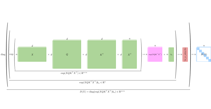
Figure 1: The visualization of the matrix $D(X)\in\mathbb{R}^{n\times n}$. Given $Q,K,V\in\mathbb{R}^{d\times d}$ and $X\in\mathbb{R}^{n\times d}$, we first compute $XQK^{\top}X^{\top}\in\mathbb{R}^{n\times n}$. Then, we find $\exp(XQK^{\top}X^{\top})\in\mathbb{R}^{n\times n}$. After that, we multiply $\exp(XQK^{\top}X^{\top})\in\mathbb{R}^{n\times n}$ with the vector ${\bf 1}_{n}\in\mathbb{R}^{n}$. Finally, we use $\operatorname{diag}(\cdot)$ to transform $\exp(XQK^{\top}X^{\top}){\bf 1}_{n}\in\mathbb{R}^{n}$ into a diagonal matrix, which is $D(X)\in\mathbb{R}^{n\times n}$. In this figure, green matrices/vectors represent the terms that are given; the purple matrix represents the term after one operation; the red vector represents the term after two operations; the blue matrix represents the term after three operations.

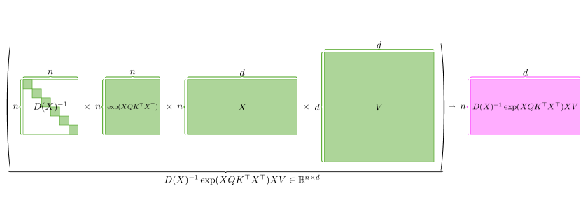
Figure 2: The visualization of the attention computation (see Eq. (15)). Since we present the visualization of how we get $D(X)\in\mathbb{R}^{n\times n}$ and $\exp(XQK^{\top}X^{\top})\in\mathbb{R}^{n\times n}$ in Figure 1, we regard them as given. Moreover, we are also given $V\in\mathbb{R}^{d\times d}$ and $X\in\mathbb{R}^{n\times d}$. We compute their product, namely $D(X)^{-1}\exp(XQK^{\top}X^{\top})XV$. In this figure, green matrices represent the terms that are given, and the purple matrix represents the term after one operation.

In [9, 14], they simplify the computation by treating $XQ$, $XK$, and $XV$ as $Q,K,V\in\mathbb{R}^{n\times d}$ so that they get

$$D^{-1}\exp(QK^{\top})V$$ (16)

where $D=\mathrm{diag}(\exp(QK^{\top}){\bf 1}_{n})$.

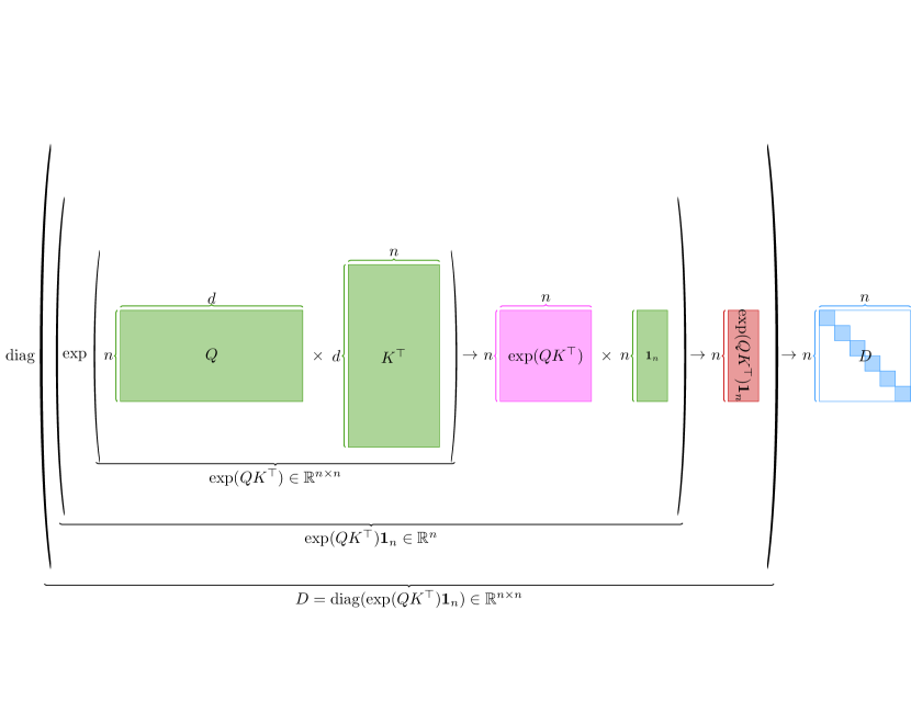
Figure 3: The visualization of the matrix $D\in\mathbb{R}^{n\times n}$. Given $Q,K,V\in\mathbb{R}^{n\times d}$, we first compute $QK^{\top}\in\mathbb{R}^{n\times n}$. Then, we find $\exp(QK^{\top})\in\mathbb{R}^{n\times n}$. After that, we multiply $\exp(QK^{\top})\in\mathbb{R}^{n\times n}$ with the vector ${\bf 1}_{n}\in\mathbb{R}^{n}$. Finally, we use $\operatorname{diag}(\cdot)$ to transform $\exp(QK^{\top}){\bf 1}_{n}\in\mathbb{R}^{n}$ into a diagonal matrix, which is $D\in\mathbb{R}^{n\times n}$. In this figure, green matrices/vectors represent the terms that are given; the purple matrix represents the term after one operation; the red vector represents the term after two operations; the blue matrix represents the term after three operations.

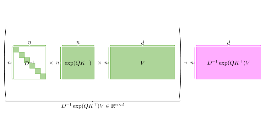
Figure 4: The visualization of the simplified version of attention computation in [9, 14] (see Eq. (16)). Since we present the visualization of how we get $D\in\mathbb{R}^{n\times n}$ and $\exp(QK^{\top})\in\mathbb{R}^{n\times n}$ in Figure 3, we regard them as given. Moreover, we are also given $V\in\mathbb{R}^{n\times d}$. We compute their product, namely $D^{-1}\exp(QK^{\top})V\in\mathbb{R}^{n\times d}$. In this figure, green matrices represent the terms that are given, and the purple matrix represents the term after one operation.

Furthermore, in [38], they simplify the attention by another strategy, namely

$$D^{-1}\exp(QK^{\top}),$$ (17)

where $D,Q,K$ are defined same as above.

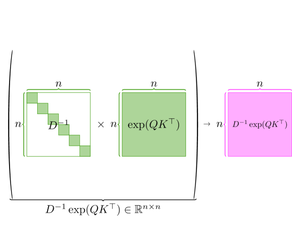
Figure 5: The visualization of the simplified version of attention computation in [38] (see Eq. (17)). Since we present the visualization of how we get $D\in\mathbb{R}^{n\times n}$ and $\exp(QK^{\top})\in\mathbb{R}^{n\times n}$ in Figure 3, we regard them as given. We compute their product, namely $D^{-1}\exp(QK^{\top})\in\mathbb{R}^{n\times n}$. In this figure, green matrices represent the terms that are given, and the purple matrix represents the term after one operation.

In addition, in [29], the attention is simplified into the form of

$$D^{-1}\exp(KK^{\top}),$$ (18)

where $D,Q,K$, for $(K=Q)$, are defined same as above.

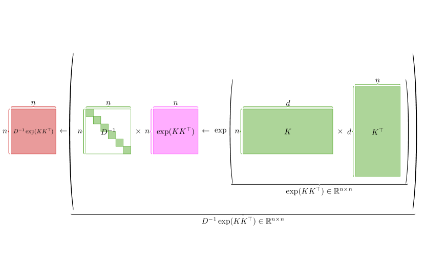
Figure 6: The visualization of the simplified version of attention computation in [29] (see Eq. (18)). Since we present the visualization of how we get $D\in\mathbb{R}^{n\times n}$ in Figure 3, we regard it as given. We are also given that $K\in\mathbb{R}^{n\times d}$, which implies that $K^{\top}\in\mathbb{R}^{d\times n}$. First, we compute their product, namely $KK^{\top}\in\mathbb{R}^{n\times n}$. Then, we find $\exp(KK^{\top})\in\mathbb{R}^{n\times n}$. Finally, we multiply $D^{-1}\in\mathbb{R}^{n\times n}$ with $\exp(KK^{\top})\in\mathbb{R}^{n\times n}$, which gives us $D^{-1}\exp(KK^{\top})\in\mathbb{R}^{n\times n}$. In this figure, green matrices represent the terms that are given; the purple matrix represents the term after one operation; the red matrix represents the term after two operations.

In this work, we provide a simplification of Eq. (15) from a different perspective, by ignoring the factor of $D^{-1}$ and $\exp$, so that we can get

$$XQK^{\top}X^{\top}XV$$

Further, we merge $QK^{\top}$ into one matrix $W$ and consider one column of $V$ a time,

$$XWX^{\top}Xv$$ (19)

where $v$ is a column of $V$.

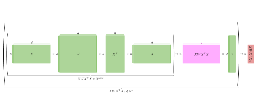
Figure 7: The visualization of the simplified version of attention computation that we analyze in this paper (see Eq. (19)). We are given that $X\in\mathbb{R}^{n\times d}$, $W\in\mathbb{R}^{d\times d}$, and $v\in\mathbb{R}^{d}$. First, we compute the product of the matrices, namely $XWX^{\top}X\in\mathbb{R}^{n\times d}$. Then, we multiply $XWX^{\top}X\in\mathbb{R}^{n\times d}$ with the vector $v\in\mathbb{R}^{d}$, which gives us $XWX^{\top}Xv\in\mathbb{R}^{n}$ In this figure, green matrices represent the terms that are given; the purple matrix represents the term after one operation; the red matrix represents the term after two operations.

Thus, we can obtain the following definition of attention computation.

Definition A.7.

Given $X\in\mathbb{R}^{n\times d}$, $W\in\mathbb{R}^{d\times d}$ and $y\in\mathbb{R}^{n}$, the goal is to solve the following regression problem

$$\min_{v\in\mathbb{R}^{d}}\|XWX^{\top}X\cdot v-y\|_{2}^{2}$$

Lemma A.8.

Solving problem A.7 is equivalent to problem A.9.

Proof.

Let $W=UU^{\top}$.

We define $\widetilde{X}$ and $\widetilde{v}$ as follows

$$\widetilde{X}:=XU$$

$$\widetilde{v}:=U^{-1}v$$

Then we have $X=\widetilde{X}U^{-1}$.

$$\min_{v\in\mathbb{R}^{d}}\|XWX^{\top}X\cdot v-y\|_{2}^{2}$$

is equivalent to

$$\min_{v\in\mathbb{R}^{d}}\|\widetilde{X}\widetilde{X}^{\top}\widetilde{X}U^{-1}v-y\|_{2}^{2}$$

is equivalent to

$$\min_{\widetilde{v}\in\mathbb{R}^{d}}\|\widetilde{X}\widetilde{X}^{\top}\widetilde{X}\widetilde{v}-y\|_{2}^{2}$$

Here we use that $U$ is full rank. ∎

The above problem is equivalent to solving the following problem

Definition A.9.

Given $X\in\mathbb{R}^{n\times d}$, $y\in\mathbb{R}^{n}$. The goal is to solve

$$\min_{v\in\mathbb{R}^{d}}\|XX^{\top}Xv-y\|_{2}^{2}$$

Appendix B Preliminary about Exp of Inner Product Kernel

In Section B.1, we provide a formal definition of the attention kernel. In Section B.2, we analyze the properties of the attention kernel.

B.1 Definition of Attention Kernel

Here, we start to present the definitions of the Gaussian Kernel and the Attention Kernel.

In this work, we will focus on $\exp(\langle,\rangle)$ inner product. It is similar to the Gaussian kernel, let us first review the definition of the Gaussian Kernel

Definition B.1 (Gaussian Kernel ).

Let $x,y\in\mathbb{R}^{d}$ be two data points.

Let $X\in\mathbb{R}^{d\times n}$.

Let $x_{i}$ be the $i$-th column of $X$.

Let $x_{j}$ be the $j$-th column of $X$.

We say $G$ is the Gaussian kernel between $x$ and $y$ if

$$G(x,y)=\exp(-\|x-y\|_{2}^{2}/2).$$

We say $G$ is the Gaussian kernel on $X$ if

$$G_{i,j}=\exp(-\|x_{i}-x_{j}\|_{2}^{2}/2).$$

We define the Attention kernel as follows

Definition B.2 (Attention Kernel).

Let $x,y\in\mathbb{R}^{d}$ be two data points.

Let $X\in\mathbb{R}^{d\times n}$.

Let $x_{i}$ be the $i$-th column of $X$.

Let $x_{j}$ be the $j$-th column of $X$.

We say $G$ is the Attention kernel between $x$ and $y$ if

$$G(x,y)=\exp(\langle x,y\rangle).$$

We say $G$ is the Attention kernel on $X$ if

$$G_{i,j}=\exp(\langle x_{i},x_{j}\rangle),$$

B.2 Property of Attention Kernel

After we define the attention kernel, we start to analyze its properties.

Fact B.3.

Let $B$ be a PSD matrix in $\mathbb{R}^{n\times n}$.

Then we have

$$B_{i,i}B_{j,j}\geq B_{i,j}^{2},~{}~{}~{}\forall i,j\in[n]\times[n]$$

Proof.

Let $x=a\cdot e_{i}+b\cdot e_{j}$.

For all arbitrary $a,b\in\mathbb{R}$, we can get

$$0\leq ~{}x^{\top}Bx$$

$$= ~{}\begin{bmatrix}a&b\end{bmatrix}\begin{bmatrix}B_{i,i}&B_{i,j}\\ B_{j,i}&B_{j,j}\end{bmatrix}\begin{bmatrix}a\\ b\end{bmatrix},$$ (20)

where the first step follows from the fact that $B$ is a PSD matrix and the second step follows from expanding the equation.

Note that for all arbitrary $a,b\in\mathbb{R}$, Eq. (B.2) holds.

Therefore,

$$\det(\begin{bmatrix}B_{i,i}&B_{i,j}\\ B_{j,i}&B_{j,j}\end{bmatrix})\geq 0$$

which is equivalent to say $B_{i,i}B_{j,j}\geq B_{i,j}^{2}$. ∎

Lemma B.4.

Let $X\in\mathbb{R}^{n\times d}$.

We define Attention kernel

$$A:=\exp(XX^{\top})\in\mathbb{R}^{n\times n}$$

where $\exp(\cdot)$ is applied entrywise.

Let $\epsilon\in(0,0.1)$ and $r>0$ satisfying the following conditions

• Condition 1. $\epsilon\leq\frac{1}{4}\exp(-4r).$

• Condition 2. $A_{i,j}\in[\exp(-r),\exp(r)]$ for $i,j\in[n]\times[n]$.

• Condition 3. $(1-\epsilon)\cdot A\preceq B\preceq(1+\epsilon)\cdot A$.

Then, we have

$$B_{i,j}\in[(1-\sqrt{\epsilon})\exp(-r),(1+\epsilon)\exp(r)].$$

Proof.

$B-(1-\epsilon)\cdot A$ is a PSD matrix.

Thus, we have

$$|B_{i,j}-(1-\epsilon)\cdot A_{i,j}|\leq ~{}\sqrt{(B_{i,i}-(1-\epsilon)\cdot A_{i,i})(B_{j,j}-(1-\epsilon)\cdot A_{j,j})}$$

$$\leq ~{}2\epsilon\sqrt{A_{i,i}A_{j,j}}$$

$$\leq ~{}2\epsilon\exp(r)$$ (21)

where the 1st step is by Lemma B.3, the 2nd step is due to $B_{i,i}\leq(1+\epsilon)A_{i,i}$ (By condition 3 in Lemma statement), and the 3rd step is because of the definition of $A_{i,j}$ from the lemma statement.

Based on the second condition from the Lemma statement, we have

$$(1-\epsilon)\cdot A_{i,j}\in ~{}[(1-\epsilon)\cdot\exp(-r),(1-\epsilon)\cdot\exp(r)],$$ (22)

Combining Eq. (B.2) and Eq. (22), we have

$$B_{i,j}\in ~{}[(1-\epsilon)\exp(-r)-2\epsilon\exp(r),(1+\epsilon)\exp(r)]$$ (23)

By using $(1+\epsilon)\cdot A-B$ is a PSD matrix, we may do a symmetric argument as follows:

$$B_{i,j}\in ~{}[(1+\epsilon)\exp(-r)-2\epsilon\exp(r),(1+3\epsilon)\exp(r)].$$ (24)

The intersection of Eq. (23) and Eq. (24) gives us:

$$B_{i,j}\in ~{}[(1+\epsilon)\exp(-r)-2\epsilon\exp(r),(1+\epsilon)\exp(r)]$$

We know that

$$(1+\epsilon)\exp(-r)-2\epsilon\exp(r)\geq ~{}\exp(-r)-2\epsilon\exp(r)$$

$$= ~{}\exp(-r)-2\sqrt{\epsilon}\cdot\sqrt{\epsilon}\cdot\exp(r)$$

$$\geq ~{}\exp(-r)-2\cdot\sqrt{\epsilon}\cdot\frac{1}{2}\exp(-2r)\cdot\exp(r)$$

$$= ~{}\exp(-r)-\sqrt{\epsilon}\exp(-r)$$

$$= ~{}(1-\sqrt{\epsilon})\cdot\exp(-r)$$

where the first step follows from $\epsilon\geq 0$, the second step follows from simple algebra, the third step follows from $\sqrt{\epsilon}\leq\frac{1}{2}\exp(-2r)$ (by condition 1 in Lemma statement), the fourth step follows from simple algebra, and the last step follows from simple algebra.

Thus, we have

$$B_{i,j}\in ~{}[(1-\sqrt{\epsilon})\exp(-r),(1-\epsilon)\exp(r)].$$

This completes the proof. ∎

Appendix C Preliminary about Standard Sketching

In Section C.1, we provide two formal definitions about the sketching matrices. In Section C.2, we introduce the formal definition of “subspace embedding”. In Section C.3, we interpret analyze the property of subsample embedding by different matrices. In Section C.4, we provide the definition of the Frobenius norm approximate matrix product.

C.1 Sketching Matrices

Now, we define subsampled randomized Hadamard transform ($\mathsf{SRHT}$) as follows.

Definition C.1 (Subsampled Randomized Hadamard Transform ($\mathsf{SRHT}$), see [55, 101]).

Let $H$ be the Hadamard matrix in $\mathbb{R}^{d\times d}$ (see Definition A.3).

Let $D$ be a diagonal matrix in $\mathbb{R}^{d\times d}$, which satisfies that each diagonal entry is either $-1$ or $1$ with the same probability.

Let $P$ be a matrix in $\{0,1\}^{m\times d}$, where each row of $P$ contains only one $1$ at a random entry.

We define the matrix $S\in\mathbb{R}^{m\times d}$ as

$$S:=\frac{1}{\sqrt{m}}PHD$$

and call $S$ the $\mathsf{SRHT}$ matrix.

We define $\mathsf{TensorSRHT}$ as follows:

Definition C.2 (Tensor Subsampled Randomized Hadamard Transform ($\mathsf{TensorSRHT}$), Definition 2.9 in [83]).

Let $P$ be a matrix in $\{0,1\}^{m\times d}$, where each row of $P$ contains only one $1$ at a random entry. $P$ can be regarded as the sampling matrix.

Let $H$ be the Hadamard matrix in $\mathbb{R}^{d\times d}$ (see Definition A.3).

Let $D_{1}$ and $D_{2}$ be diagonal matrices in $\mathbb{R}^{d\times d}$, which satisfy that each diagonal entry is either $-1$ or $1$ with the same probability. $D_{1}$ and $D_{2}$ are independent.

Then, we define $\mathsf{TensorSRHT}$ as a function $S:\mathbb{R}^{d}\times\mathbb{R}^{d}\to\mathbb{R}^{m}$, which is defined as

$$S:=\frac{1}{\sqrt{m}}P\cdot(HD_{1}\otimes HD_{2}).$$

C.2 Subspace embedding

We define subspace embedding as follows.

Definition C.3 (Subspace embedding $\mathsf{SE}(n,d,\epsilon,\delta)$).

Given a matrix $A\in\mathbb{R}^{n\times d}$, we say $S$ is an $(n,d,\epsilon,\delta)$ subspace embedding, if

$$\Pr[(1-\epsilon)\cdot\|Ax\|_{2}\leq\|SAx\|_{2}\leq(1+\epsilon)\cdot\|Ax\|_{2}]\geq 1-\delta.$$

We define a more general version of subspace embedding, this can be viewed as a variation of Definition 2 in [5].

Definition C.4 (Stable Rank Subspace Embedding $\mathsf{SSE}(n,d,\epsilon,\delta,\mu)$).

Given $\epsilon$, $\delta$, $\mu>0$ and integers $d$, $n\geq 1$, an $(n,d,\epsilon,\delta,\mu)$-Stable Rank Subspace Embedding ($\mathsf{SSE}$) is a distribution $\mathcal{D}$ over $m\times n$ matrices (for arbitrary $m$) such that, for $A\in\mathbb{R}^{n\times d}$ with $\mathrm{srank}(A^{\top}A)\leq\mu$, the following holds:

$$\Pr_{\Pi\sim D}[(1-\epsilon)\cdot(A^{\top}A)\preceq A^{\top}\Pi^{\top}\Pi A\preceq(1+\epsilon)\cdot(A^{\top}A)]\geq 1-\delta.$$

C.3 Subsapace embedding by different matrices

In this section, we analyze the property of the subspace embedding: subspace embedding by different matrices

Lemma C.5.

Given a matrix $A\in\mathbb{R}^{n\times d}$. The matrix $S\in\mathbb{R}^{m\times n}$ is an $\mathsf{SE}(n,d,\epsilon,\delta)$ subspace embedding if any of the following condition holds

• Let $S\in\mathbb{R}^{m\times n}$ denote a $\mathsf{SRHT}$ matrix with $m=O(\epsilon^{-2}d\log(n/\delta))$ rows. In addition, $SA$ can be computed in $O(nd\log(n/\delta))$ time.

• Let $S\in\mathbb{R}^{m\times n}$ denote $\mathsf{OSNAP}$ matrix with $m=O(\epsilon^{-2}d\log(d/\delta))$ rows and column sparsity $s=O(\epsilon^{-1}\log(d/\delta))$. In addition, $SA$ can be computed in $O(s\cdot\operatorname{nnz}(A))$ time.

C.4 Approximate Matrix Product

Here, we define the Frobenius Norm Approximate Matrix Product as follows.

Definition C.6 (Frobenius Norm Approximate Matrix Product).

Let $A\in\mathbb{R}^{n\times d_{1}},B\in\mathbb{R}^{d_{2}\times n}$ be two matrices. We say $S$ is Frobenius Norm Approximate Matrix Product $\mathsf{FAMP}(n,\epsilon,\delta)$ with respect to $A,B$ if

$$\Pr[\|A^{\top}B-A^{\top}S^{\top}SB\|_{F}\leq\epsilon\|A\|_{F}\|B\|_{F}]\geq 1-\delta$$

Appendix D Preliminary about High Precision Sketching

In Section D.1, we explain more useful facts. In Section D.2, we explain the small sanity check lemma. In Section D.3, we analyze the property of well-conditioned PSD regression. In Section D.4, we analyze the forward error for simple matrices. In Section D.5, we study the forward error for PSD matrices.

D.1 Facts

In this section, we introduce more facts.

Fact D.1.

The following two conditions are equivalent

• for all unit vector $x$, $(1-\epsilon)\leq\|Ax\|_{2}^{2}\leq(1+\epsilon)$

• $\|A^{\top}A-I\|\leq\epsilon$

Proof.

We know that,

$$\|A^{\top}A-I\|\leq\epsilon$$

is equivalent to

$$-\epsilon\leq x^{\top}(A^{\top}A-I)x\leq\epsilon,~{}~{}~{}\forall\|x\|_{2}=1$$

which is equivalent to

$$1-\epsilon\leq x^{\top}A^{\top}Ax\leq 1+\epsilon,~{}~{}~{}\forall\|x\|_{2}=1$$

which is equivalent to

$$1-\epsilon\leq\|Ax\|_{2}^{2}\leq 1+\epsilon,~{}~{}~{}\forall\|x\|_{2}=1$$

∎

D.2 Small Sanity Check Lemma

In this section, we present the small sanity check lemma.

Lemma D.2.

Given a matrix $A\in\mathbb{R}^{n\times d}$ and $b\in\mathbb{R}^{n}$, let $S\in\mathbb{R}^{n\times n}$ denote a sampling and rescaling diagonal matrix. Let $\epsilon\in(0,1)$ denote an accuracy parameter.

Suppose that

$$(1-\epsilon)\cdot A^{\top}A\preceq A^{\top}S^{\top}SA\preceq(1+\epsilon)\cdot A^{\top}A$$

Let $x^{*}\in\mathbb{R}^{d}$ denote $\arg\min_{x}\|A^{\top}Ax-b\|_{2}^{2}$ and $x^{\prime}\in\mathbb{R}^{d}$ denote $\arg\min_{x}\|A^{\top}S^{\top}SAx-b\|_{2}^{2}$.

Then we have

$$\|A^{\top}Ax^{\prime}-b\|_{2}\leq\epsilon\|b\|_{2}.$$

Proof.

We define

$$\Delta_{A}:=((A^{\top}A)^{1/2}(A^{\top}S^{\top}SA)(A^{\top}A)^{1/2}-I)$$ (25)

From the assumption in Lemma statement, we have

$$-\epsilon I\preceq\Delta_{A}\preceq\epsilon I.$$

We have

$$\|A^{\top}Ax^{\prime}-b\|_{2}= ~{}\|A^{\top}A(A^{\top}S^{\top}SA)^{-1}b-b\|_{2}$$

$$= ~{}\|(A^{\top}A(A^{\top}S^{\top}SA)^{-1}-I)b\|_{2}$$

$$= ~{}\|(A^{\top}A)^{1/2}((A^{\top}A)^{1/2}(A^{\top}S^{\top}SA)^{-1}(A^{\top}A)^{1/2}-I)(A^{\top}A)^{-1/2}b\|_{2}$$

$$= ~{}\|(A^{\top}A)^{1/2}\Delta_{A}(A^{\top}A)^{-1/2}b\|_{2},$$

where the first step comes from the definition of $x^{\prime}$ (see from the Lemma statement), the second and the third steps are due to simple algebra, and the last step is by the definition of $\Delta_{A}$ (see Eq. (25)).

Then we have

$$~{}\|(A^{\top}A)^{1/2}\Delta_{A}(A^{\top}A)^{-1/2}b\|_{2}^{2}$$

$$= ~{}b^{\top}(A^{\top}A)^{-1/2}\Delta_{A}(A^{\top}A)^{1/2}\cdot(A^{\top}A)^{1/2}\Delta_{A}(A^{\top}A)^{-1/2}b$$

$$= ~{}b^{\top}(A^{\top}A)^{-1/2}\Delta_{A}A^{\top}A\Delta_{A}(A^{\top}A)^{-1/2}b$$

$$\leq ~{}\epsilon^{2}b^{\top}(A^{\top}A)^{-1/2}A^{\top}A(A^{\top}A)^{-1/2}b$$

$$= ~{}\epsilon^{2}\|b\|_{2}^{2}$$

where the first step follows from the definition of the $\ell_{2}$ norm, the second step follows from simple algebra, the third step follows from $\Delta_{A}A^{\top}A\Delta_{A}\preceq\epsilon^{2}A^{\top}A$, and the last step follows from simple algebra (associative property of matrix multiplication).

Finally, we obtain,

$$\|A^{\top}Ax^{\prime}-b\|_{2}\leq ~{}\epsilon\|b\|_{2}.$$

Thus, we complete the proof. ∎

D.3 Well-conditioned PSD Regression

In this section, we consider the property of positive semidefinite (PSD) matrix.

Lemma D.3 (Well-conditioned PSD regression, Lemma B.2 in [13]).

Consider the regression problem

$$\min_{x\in\mathbb{R}^{d}}\|Bx-y\|_{2}^{2}.$$

Suppose $B\in\mathbb{R}^{d\times d}$ is a PSD matrix with

$$\frac{3}{4}\leq\|Bx\|_{2}\leq\frac{5}{4},~{}~{}~{}~{}\forall x\text{~{}such~{}that~{}}\|x\|_{2}=1.$$

Using gradient descent update

$$x_{t+1}=x_{t}-B^{\top}(Bx_{t}-y).$$

Then, after $t$ iterations, we obtain

$$\|B(x_{t}-x^{*})\|_{2}\leq c^{t}\|B(x_{0}-x^{*})\|_{2}$$

for some constant $c\in(0,0,9]$.

Proof.

The gradient at time $t$ is $B^{\top}(Bx_{t}-y)$ and

$$x_{t+1}=x_{t}-B^{\top}(Bx_{t}-y),$$ (26)

so we have

$$\|Bx_{t+1}-Bx^{*}\|_{2}= ~{}\|B(x_{t}-B^{\top}(Bx_{t}-y))-Bx^{*}\|_{2}$$

$$= ~{}\|B(x_{t}-x^{*})-BB^{\top}Bx_{t}+BB^{\top}Bx^{*}\|_{2}$$

$$= ~{}\|B(x_{t}-x^{*})-BB^{\top}B(x_{t}-x^{*})\|_{2}$$

$$= ~{}\|(I-BB^{\top})B(x_{t}-x^{*})\|_{2}$$

$$\leq ~{}\|(I-BB^{\top})\|\cdot\|B(x_{t}-x^{*})\|_{2}$$

$$\leq ~{}\frac{9}{16}\|B(x_{t}-x^{*})\|_{2},$$

where the first step follows from Eq. (26), the second step follows from $B^{\top}Bx^{*}=B^{\top}y$, the third step follows from simple algebra, the fourth step follows from simple algebra, the fifth step follows from $\|Ax\|_{2}\leq\|A\|\cdot\|x\|_{2}$, and the last step follows from the fact that the eigenvalue of $BB^{\top}$ belongs to $[\frac{9}{16},\frac{25}{16}]$ by our assumption.

Thus we complete the proof. ∎

D.4 Forwarded Error for Simple Matrix

In this section, we analyze the forwarded error for the simple matrix.

Lemma D.4 (Lemma 5.5 in [39]).

Given a matrix $A\in\mathbb{R}^{n\times d}$, a vector $b\in\mathbb{R}^{n}$. Suppose there is a vector $x^{\prime}\in\mathbb{R}^{d}$ such that

$$\|Ax^{\prime}-b\|_{2}\leq(1+\epsilon_{1})\min_{x\in\mathbb{R}^{d}}\|Ax-b\|_{2}$$

Let $x_{*}$ denote the exact solution to the regression problem, then it holds that

$$\|x^{\prime}-x_{*}\|_{2}\leq O(\sqrt{\epsilon_{1}})\cdot\frac{1}{\sigma_{\min}(A)}\cdot\|Ax_{*}-b\|_{2}.$$

For the completeness, we still provide a proof.

Proof.

Note that

$$\|Ax^{\prime}-Ax_{*}\|_{2}=\|Ax^{\prime}-b-(Ax_{*}-b)\|_{2},$$

so we can perform the following decomposition:

$$\|A(x^{\prime}-x_{*})\|_{2}^{2}= ~{}\|Ax^{\prime}-b-(Ax_{*}-b)\|_{2}^{2}$$

$$= ~{}\|Ax^{\prime}-b\|_{2}^{2}-\|Ax_{*}-b\|_{2}^{2}$$

$$\leq ~{}(1+\epsilon_{1})^{2}\|Ax_{*}-b\|_{2}^{2}-\|Ax_{*}-b\|_{2}^{2}$$

$$\leq ~{}4\epsilon_{1}\cdot\|Ax_{*}-b\|_{2}^{2},$$ (27)

where the first step follows from simple algebra, the second step follows from the Pythagorean theorem, the third step follows from the assumption in Lemma statement, and the fourth step follows from simple algebra.

Assuming $A$ has full column rank, then $A^{\dagger}A=I$.

Therefore, we have

$$\|x^{\prime}-x_{*}\|_{2}= ~{}\|A^{\dagger}A(x^{\prime}-x_{*})\|_{2}$$

$$\leq ~{}\|A(x^{\prime}-x_{*})\|_{2}\cdot\|A^{\dagger}\|$$

$$\leq ~{}2\sqrt{\epsilon_{1}}\cdot\|Ax_{*}-b\|_{2}\cdot\|A^{\dagger}\|$$

$$= ~{}\frac{2\sqrt{\epsilon_{1}}}{\sigma_{\min}(A)}\cdot\|Ax_{*}-b\|_{2},$$

where the first step follows from $A^{\dagger}A=I$, the second step follows from $\|ABx\|_{2}\leq\|Ax\|_{2}\|B\|$, the third step follows from Eq. (D.4), and the last step follows from $\|A^{\dagger}\|=\|A^{-1}\|=\frac{1}{\sigma_{\min}(A)}$ ∎

D.5 Forwarded Error PSD Matrices

In this section, we study the forwarded error for PSD matrices.

Lemma D.5 (PSD version of Lemma D.4).

Given a matrix $A\in\mathbb{R}^{n\times d}$, a vector $b\in\mathbb{R}^{d}$. Suppose there is a vector $x^{\prime}\in\mathbb{R}^{d}$ such that

$$\|A^{\top}Ax^{\prime}-b\|_{2}\leq\epsilon_{2}\|b\|_{2}$$

Let $x_{*}$ denote the exact solution to the regression problem, then it holds that

$$\|x^{\prime}-x_{*}\|_{2}\leq\epsilon_{2}\cdot\frac{1}{\sigma_{\min}(A)^{2}}\cdot\|b\|_{2}.$$

For completeness, we still provide proof.

Proof.

Note that

$$\|A^{\top}Ax^{\prime}-A^{\top}Ax_{*}\|_{2}=\|(A^{\top}Ax^{\prime}-b)-(A^{\top}Ax_{*}-b)\|_{2},$$

so we can perform the following decomposition:

$$\|A^{\top}A(x^{\prime}-x_{*})\|_{2}^{2}= ~{}\|(A^{\top}Ax^{\prime}-b)-(A^{\top}Ax_{*}-b)\|_{2}^{2}$$

$$= ~{}\|A^{\top}Ax^{\prime}-b\|_{2}^{2}-\|A^{\top}Ax_{*}-b\|_{2}^{2}$$

$$\leq ~{}\epsilon_{2}^{2}\|b\|_{2}^{2}$$ (28)

where the first step follows from simple algebra, the second step follows from the Pythagorean theorem, the third step follows from the assumption in Lemma statement.

Assuming $A$ has full column rank, then $(A^{\top}A)^{\dagger}(A^{\top}A)=I$.

Therefore, we have

$$\|x^{\prime}-x_{*}\|_{2}= ~{}\|(A^{\top}A)^{\dagger}A^{\top}A(x^{\prime}-x_{*})\|_{2}$$

$$\leq ~{}\|A^{\top}A(x^{\prime}-x_{*})\|_{2}\cdot\|(A^{\top}A)^{\dagger}\|$$

$$\leq ~{}\epsilon_{2}\cdot\|b\|_{2}\cdot\|(A^{\top}A)^{\dagger}\|$$

$$= ~{}\epsilon_{2}\cdot\sigma_{\min}(A)^{-2}\|b\|_{2}$$

where the first step follows from $(A^{\top}A)^{\dagger}(A^{\top}A)=I$, the second step follows from $\|ABx\|_{2}\leq\|Ax\|_{2}\|B\|$, the third step follows from Eq. (D.5), and the last step follows from Fact A.4. ∎

Appendix E From Attention Regression to Multiple Matrices Regression

In Section E.1, we introduce the background of the attention matrices. In Section E.2, we analyze the equivalence between $\mathsf{mid}$ version linear attention and $\mathsf{right}$ version linear attention.

E.1 Background on Attention Matrix

In this section, we review the standard attention computation model, e.g., see [9] as an example. We define attention matrix and attention computation as follows,

Definition E.1 (Attention Computation).

Given three matrices $Q,K,V\in\mathbb{R}^{n\times d}$ and outputs the following matrix

$$\operatorname{\mathrm{Att}}(Q,K,V):=D^{-1}AV$$

where $A\in\mathbb{R}^{n\times n}$

$$A:=\exp(QK^{\top})$$

and $D\in\mathbb{R}^{n\times n}$ is a diagonal matrix

$$D:=\operatorname{diag}(A{\bf 1}_{n}).$$

In actual Large Language Models (LLMs), we actually consider the following computation problem,

Definition E.2 (An alternative Attention Computation).

Given three matrices $Q,K,V\in\mathbb{R}^{d\times d}$.

For any input $X\in\mathbb{R}^{n\times d}$, we can define function $\operatorname{\mathrm{Att}}:\mathbb{R}^{n\times d}\rightarrow\mathbb{R}^{n\times d}$

$$\operatorname{\mathrm{Att}}(X):=D^{-1}AXV$$

where $A\in\mathbb{R}^{n\times n}$

$$A:=\exp(XQK^{\top}X^{\top})$$

and $D\in\mathbb{R}^{n\times n}$ is a diagonal matrix

$$D:=\operatorname{diag}(A{\bf 1}_{n}).$$

Mathematically, we can merge $QK^{\top}\in\mathbb{R}^{d\times d}$ into one unknow $d\times d$ matrix which is called $U\in\mathbb{R}^{d\times d}$.

Definition E.3 (Soft-max Attention Regression).

Let $\exp()$ denote the entry-wise exponential function. Given data points $\{x_{1},\cdots,x_{n}\}\subset\mathbb{R}^{d}$. Let $X=\begin{bmatrix}x_{1}&x_{2}&\cdots&x_{n}\end{bmatrix}^{\top}\in\mathbb{R}^{n\times d}$ denote that data matrix. Let $Y\in\mathbb{R}^{n\times d}$ denote the labels corresponding to $x_{1},\cdots,x_{n}$. Assume $v\in\mathbb{R}^{d}$ is fixed.

For $U\in\mathbb{R}^{d\times d}$, we define the loss function

$$L(U,V):=\|Y-D^{-1}AXV\|_{F}^{2}.$$

where matrix $A\in\mathbb{R}^{n\times n}$ and diagonal matrix $D\in\mathbb{R}^{n\times n}$ is defined as follows:

$$A:=\exp(XUX^{\top}),~{}~{}~{}D=\operatorname{diag}(A{\bf 1}_{n}).$$

If we drop the nonlinear units in the regression problem (e.g. $D^{-1}\exp()$ which is soft-max operator), then we can obtain

$$L(U,V)=\|Y-XUX^{\top}XV\|_{F}^{2}.$$

Usually, the standard way to solve this minimization is using alternative minimization [45, 39]. One step we fixed $U$ to solve $V$, and the other step, we fixed $V$ and to solve for $U$. This motivates us to define Definition E.4 and Definition E.5.

E.2 Equivalence Between $\mathsf{mid}$ Version Linear Attention and $\mathsf{right}$ Version Linear Attention

We define a simplified version attention regression problem which is essentially linear model. We call it is $\mathsf{mid}$ because the unknown variables we are trying to recover lies in the the middle.

Definition E.4 (Linear Attention Regression $\mathsf{mid}$ version).

Given data points $\{x_{1},\cdots,x_{n}\}\subset\mathbb{R}^{d}$, we let $X=\begin{bmatrix}x_{1}&x_{2}&\cdots&x_{n}\end{bmatrix}^{\top}\in\mathbb{R}^{n\times d}$ denote that data matrix.

Let $Y\in\mathbb{R}^{n\times d}$ denote the labels corresponding to $x_{1},\cdots,x_{n}$.

For $U\in\mathbb{R}^{d\times d}$, we define the loss function

$$L_{\mathsf{mid}}(U):=\|\underbrace{Y}_{n\times d}-\underbrace{X}_{n\times d}U\underbrace{X^{\top}}_{d\times n}\underbrace{X}_{n\times d}\|_{F}^{2}.$$

Similarly, we also define the $\mathsf{right}$ version of linear attention regression.

Definition E.5 (Linear Attention Regression $\mathsf{mid}$ version).

Given data points $\{x_{1},\cdots,x_{n}\}\subset\mathbb{R}^{d}$, we let $X=\begin{bmatrix}x_{1}&x_{2}&\cdots&x_{n}\end{bmatrix}^{\top}\in\mathbb{R}^{n\times d}$ denote that data matrix.

Let $Y\in\mathbb{R}^{n\times d}$ denote the labels corresponding to $x_{1},\cdots,x_{n}$.

For $v\in\mathbb{R}^{d\times d}$, we define the loss function

$$L_{\mathsf{right}}(V):=\|\underbrace{Y}_{n\times d}-\underbrace{X}_{n\times d}\underbrace{X^{\top}}_{d\times n}\underbrace{X}_{n\times d}\underbrace{V}_{d\times d}\|_{F}^{2}.$$

Lemma E.6.

If we restrict the output matrix to be PD matrix in Definition E.4 and Definition E.5. Then the $\mathsf{mid}$ version of linear attention regression and $\mathsf{right}$ version of linear attention regression are equivalent.

Proof.

The proof is straightforward, since the $XU^{1/2}$ in $L_{\mathsf{mid}}$ is the $X$ in $L_{\mathsf{right}}$. The $V$ in $L_{\mathsf{right}}$ is $U^{-1/2}$ (where $U$ is in $L_{\mathsf{mid}}$). ∎

Appendix F Linear Regression

In this section, we present the fast linear regression algorithm and analyze the property of it.

Algorithm 1 Fast Linear Regression. This solves $\min_{x}\|Ax-b_{1}\|_{2}$

1:procedure FastLinearRegression($A\in\mathbb{R}^{n\times d},b_{1}\in\mathbb{R}^{n},n\in\mathbb{Z}_{+},d\in\mathbb{Z}_{+},\epsilon_{1}\in(0,1),\delta_{1}\in(0,1)$)

2:     Compute a subspace embedding $S_{1}A$ $\triangleright$ Let $S_{1}$ denote a $\mathsf{SE}(n,d,\epsilon_{\mathrm{ose}}=0.1,\delta_{\mathrm{ose}}=\delta_{1}/2)$

3:     Compute $R$ such that $S_{1}AR$ are orthonormal columns via QR decomposition $R\in\mathbb{R}^{d\times d}$

4:     $T_{1}\leftarrow\Theta(\log(1/\epsilon_{1}))$

5:     $z_{0}\leftarrow\arg\min_{x}\|SARx-Sb_{1}\|_{2}$

6:     $t\leftarrow 0$

7:     while $\|ARz_{t}-b_{1}\|_{2}\geq\epsilon_{1}$ do

8:         $z_{t+1}\leftarrow z_{t}-(R^{\top}A^{\top})(ARz_{t}-b_{1})$

9:         $t\leftarrow t+1$

10:     end while

11:     return $Rz_{t}$

12:end procedure

Lemma F.1 (Dense and high accuracy regression, Lemma 5.4 in [39]).

Given a matrix $A\in\mathbb{R}^{n\times d}$ and a vector $b_{1}\in\mathbb{R}^{n}$, let $\epsilon_{1}\in(0,0.1)$ and $\delta_{1}\in(0,0.1)$, there exists an algorithm that takes time

$$O((nd+d^{3})\cdot\log(1/\epsilon_{1})\cdot\log^{2}(n/\delta_{1}))$$

and outputs $x^{\prime}\in\mathbb{R}^{d}$ such that

$$\|Ax^{\prime}-b_{1}\|_{2}\leq(1+\epsilon_{1})\min_{x\in\mathbb{R}^{d}}\|Ax-b_{1}\|_{2}$$

holds with probability $1-\delta_{1}$.

Proof.

Let us analyze Algorithm 1, first on its convergence then on its runtime.

Note that the $S$ we choose is an $(\epsilon_{\mathrm{ose}},\delta_{\mathrm{ose}})$-oblivious subspace embedding. Since $SA=QR^{-1}$ where $Q$ is orthonormal, we know the singular values of $AR$ are between $[1-\epsilon_{\mathrm{ose}},1+\epsilon_{\mathrm{ose}}]$.

Let $AR=U\Sigma V^{\top}$ be the SVD of $AR$ and $z^{*}$ denote the optimal solution to the regression $\min_{x\in\mathbb{R}^{d}}\|ARx-b_{1}\|_{2}$.

Let us consider

$$AR(z_{t+1}-z^{*})= ~{}AR(z_{t}+R^{\top}A^{\top}(b_{1}-ARz_{t})-z^{*})$$

$$= ~{}AR(z_{t}-z^{*})+ARR^{\top}A^{\top}b_{1}-ARR^{\top}A^{\top}ARz_{t}$$

$$= ~{}AR(z_{t}-z^{*})+ARR^{\top}A^{\top}ARz^{*}-ARR^{\top}A^{\top}ARz_{t}$$

$$= ~{}(AR-ARR^{\top}A^{\top}AR)(z_{t}-z^{*})$$

$$= ~{}(U\Sigma V^{\top}-U\Sigma^{3}V^{\top})(z_{t}-z^{*}),$$ (29)

where the first step follows from the definition of $z_{t+1}$ from Algorithm 1, the second step follows from simple algebra, the third step follows from $b_{1}=ARz^{*}$, the fourth step follows from simple algebra, the last step follows from the SVD, $AR=U\Sigma V^{\top}$.

Therefore,

$$\|AR(z_{t+1}-z^{*})\|_{2}= ~{}\|(U\Sigma V^{\top}-U\Sigma^{3}V^{\top})(z_{t}-z^{*})\|_{2}$$

$$= ~{}\|(\Sigma-\Sigma^{3})V^{\top}(z_{t}-z^{*})\|_{2}$$

$$\leq ~{}O(\epsilon_{\mathrm{ose}})\cdot\|V^{\top}(z_{t}-z^{*})\|_{2}$$

$$\leq ~{}\frac{O(\epsilon_{\mathrm{ose}})}{1-\epsilon_{\mathrm{ose}}}\|\Sigma V^{\top}(z_{t}-z^{*})\|_{2}$$

$$= ~{}O(\epsilon_{\mathrm{ose}})\cdot\|\Sigma V^{\top}(z_{t}-z^{*})\|_{2}$$

$$= ~{}O(\epsilon_{\mathrm{ose}})\cdot\|U\Sigma V^{\top}(z_{t}-z^{*})\|_{2}$$

$$= ~{}O(\epsilon_{\mathrm{ose}})\cdot\|AR(z_{t}-z^{*})\|_{2},$$

where the first step follows from Eq. (F), the second step follows from $U^{\top}U=I$, the third step follows from $\|AB\|\leq\|A\|\cdot\|B\|$, the fourth step follows from $(1-\epsilon_{\mathrm{ose}})\leq\|\Sigma\|$, the fifth step follows from $\epsilon_{\mathrm{ose}}\in(0,0.1)$, the sixth step follows from $U^{\top}U=I$, and the last step follows from the SVD, $AR=U\Sigma V^{\top}$.

This means the error shrinks by a factor of $O(\epsilon_{\mathrm{ose}})$ per iteration. After $T=O(\log(1/\epsilon_{1}))$ iterations, we have

$$\|AR(z_{T}-z^{*})\|_{2}\leq ~{}O(\epsilon_{1})\cdot\|AR(z_{0}-z^{*})\|_{2},$$ (30)

and recall for initial solution $z_{0}$, we have

$$\|ARz_{0}-b_{1}\|_{2}\leq ~{}(1+\epsilon_{\mathrm{ose}})\cdot\|ARz^{*}-b_{1}\|_{2}.$$

The above equation implies that

$$\|ARz_{0}-b_{1}\|_{2}^{2}-\|ARz^{*}-b_{1}\|_{2}^{2}\leq O(\epsilon_{\mathrm{ose}})\|ARz^{*}-b_{1}\|_{2}^{2}.$$ (31)

We can wrap up the proof as follows:

$$\|ARz_{T}-b_{1}\|_{2}^{2}= ~{}\|AR(z_{T}-z^{*})\|_{2}^{2}+\|ARz^{*}-b_{1}\|_{2}^{2}$$

$$\leq ~{}O(\epsilon_{1}^{2})\cdot\|AR(z_{0}-z^{*})\|_{2}^{2}+\|ARz^{*}-b_{1}\|_{2}^{2}$$

$$= ~{}O(\epsilon_{1}^{2})\cdot(\|ARz_{0}-b_{1}\|_{2}^{2}-\|ARz^{*}-b_{1}\|_{2}^{2})+\|ARz^{*}-b_{1}\|_{2}^{2}$$

$$\leq ~{}O(\epsilon_{1}^{2})\cdot(O(\epsilon_{\mathrm{ose}})\|ARz^{*}-b_{1}\|_{2}^{2})+\|ARz^{*}-b_{1}\|_{2}^{2}$$

$$= ~{}(1+O(\epsilon_{1}^{2}))\cdot\|ARz^{*}-b_{1}\|_{2}^{2},$$

where the first step follows from the Pythagorean theorem, the second step follows from Eq. (30), the third step follows from the Pythagorean theorem again, the fourth step follows from Eq. (31), and the fifth step follows from $\epsilon_{\mathrm{ose}}\leq 1$.

It remains to show the runtime. Applying $S$ to $A$ takes $O(nd\log n)$ time, the QR decomposition takes $O(m_{\mathrm{sk}}d^{2})=O(d^{3}\log^{2}(n/\delta_{\mathrm{ose}}))$ time.

Inverting $d\times d$ matrix $Q$ takes $O(d^{3})$ time. To solve for $z_{0}$, we need to multiply $SA$ with $R$ in $O(m_{\mathrm{sk}}d^{2})$ time and the solve takes $O(m_{\mathrm{sk}}d^{2})$ time as well. To implement each iteration, we multiply from right to left which takes $O(nd)$ time. Putting things together gives the desired runtime. ∎

Appendix G Fast PSD regression solver

In this section, we offer the fast PSD regression algorithm and analyze the property of it.

Algorithm 2 Fast PSD regression. This solves $\min_{x\in\mathbb{R}^{d}}\|A^{\top}Ax-b_{2}\|_{2}$

1:procedure FastPSDRegression($A\in\mathbb{R}^{n\times d},b_{2}\in\mathbb{R}^{d},n\in\mathbb{Z}_{+},d\in\mathbb{Z}_{+},\epsilon_{2}\in(0,1),\delta_{2}\in(0,1)$) $\triangleright$ Lemma G.1

2:     Compute a subspace embedding $S_{2}A$ $\triangleright$ Let $S_{2}$ denote a $\mathsf{SE}(n,d,\epsilon_{\mathrm{ose}}=0.1,\delta_{\mathrm{ose}}=\delta_{2}/2)$

3:     Compute $R$ such that $S_{2}AR$ orthonormal columns via QR decomposition $\triangleright$ $R\in\mathbb{R}^{d\times d}$

4:     $z_{0}\leftarrow{\bf 0}_{d}$

5:     $t\leftarrow 0$

6:     while $\|A^{\top}ARz_{t}-b_{2}\|_{2}\geq\epsilon_{2}$ do

7:         $z_{t+1}\leftarrow z_{t}-(R^{\top}A^{\top}AR)^{\top}(R^{\top}A^{\top}ARz_{t}-R^{\top}b_{2})$

8:         $t\leftarrow t+1$

9:     end while

10:     return $Rz_{t}$

11:end procedure

Lemma G.1 (Formal version of Lemma 4.2, Lemma B.1 in [13]).

Given a matrix $A\in\mathbb{R}^{n\times d}$, let $\kappa$ denote the condition number of $A$, i.e. $\kappa=\sigma_{\max}(A)/\sigma_{\min}(A)$, consider the following regression problem

$$\min_{x\in\mathbb{R}^{d}}\|A^{\top}Ax-b_{2}\|_{2}.$$ (32)

There is an algorithm that runs in time

$$O((nd+d^{3})\cdot\log(\kappa/\epsilon_{2})\cdot\log^{2}(n/\delta_{2})).$$

and outputs $x^{\prime}\in\mathbb{R}^{d}$ such that

$$\|A^{\top}Ax^{\prime}-b_{2}\|_{2}\leq\epsilon_{2}\|b_{2}\|_{2}$$

holds with probability $1-\delta_{2}$.

Proof.

Let $S_{2}\in\mathbb{R}^{s_{2}\times n}$ be a $\mathsf{SE}(n,d,\epsilon_{\mathrm{ose}}=0.1,\delta)$ (Definition C.3) for $A$, then with probability $1-\delta$, the following holds for any $x\in\mathbb{R}^{d}$

$$\|S_{2}Ax\|_{2}=(1\pm\epsilon_{\mathrm{ose}})\|Ax\|_{2}.$$ (33)

Suppose $R\in\mathbb{R}^{d\times d}$ is computed so that $SAR$ has orthonormal columns, e.g., via QR decomposition.

We use $R$ as a preconditioner for matrix $A$.

Formally, for any $x\in\mathbb{R}^{d}$ satisfying $\|x\|_{2}=1$, we have

$$\|ARx\|_{2}= ~{}(1\pm\epsilon_{\mathrm{ose}})\|S_{2}ARx\|_{2}$$

$$= ~{}(1\pm\epsilon_{\mathrm{ose}}),$$ (34)

where the first step follows from Eq. (33) and the second step follows from the fact that $S_{2}AR$ has orthonormal columns.

Taking the squares on both sides, we have

$$\|ARx\|_{2}^{2}=(1\pm 3\epsilon_{\mathrm{ose}}).$$

By Fact D.1, then above equation implies the following

$$\|R^{\top}A^{\top}AR-I\|\leq 3\epsilon_{\mathrm{ose}}$$

Hence, using the definition of spectral norm, we know for any $\|x\|_{2}=1$,

$$\|R^{\top}A^{\top}ARx\|_{2}\leq ~{}(1+3\epsilon_{\mathrm{ose}}),$$

Similarly, we can prove the other direction

$$\|R^{\top}A^{\top}ARx\|_{2}\geq(1-3\epsilon_{\mathrm{ose}})$$

We choose $\epsilon_{\mathrm{ose}}=0.1$, and consider the regression problem

$$\min_{z\in\mathbb{R}^{n}}\|R^{\top}A^{\top}ARz-R^{\top}b_{2}\|_{2}.$$ (35)

By lemma D.3, using gradient descent, after $T_{2}=\log{(1/\epsilon_{2})}$ iterations, we can find $z_{t}$ satisfying

$$\|R^{\top}A^{\top}AR(z_{t}-z^{*})\|_{2}\leq\epsilon\|R^{\top}A^{\top}AR(z_{0}-z^{*})\|_{2},$$ (36)

where

$$z^{*}=(R^{\top}A^{\top}AR)^{-1}R^{\top}b_{2}$$ (37)

is the optimal solution to Eq. (35).

We are going to show that

$$x_{t}=Rz_{t}$$ (38)

is an $2\kappa\epsilon$-approximate solution to the original regression problem (Eq. (32)), i.e.,

$$\|A^{\top}Ax_{t}-b_{2}\|_{2}\leq\kappa\epsilon_{2}\|b_{2}\|_{2}.$$

Loading Eq. (37) into Eq. (36), we obtain

$$\|R^{\top}A^{\top}ARz_{t}-R^{\top}b_{2}\|_{2}\leq\epsilon_{2}\|R^{\top}A^{\top}ARz_{0}-R^{\top}b_{2}\|_{2}$$

Loading the definition of $z_{0}=0$ and Eq. (38), we have

$$\|R^{\top}A^{\top}Ax_{t}-R^{\top}b_{2}\|_{2}\leq ~{}\epsilon_{2}\cdot\|R^{\top}b_{2}\|_{2}$$

$$\leq ~{}\epsilon_{2}\cdot\sigma_{\max}(R)\cdot\|b_{2}\|_{2},$$ (39)

where the second step follows from the definition of $\sigma_{\max}(R)$.

On the other hand, we have

$$\|R^{\top}A^{\top}Ax_{t}-R^{\top}b_{2}\|_{2}= ~{}\|R^{\top}(A^{\top}Ax_{t}-b_{2})\|_{2}$$

$$\geq ~{}\sigma_{\min}(R^{\top})\|A^{\top}Ax_{t}-b_{2}\|_{2},$$ (40)

where the first step follows from simple algebra and the second step follows from the definition of $\sigma_{\min}(R^{\top})$.

Putting it all together, we have

$$\|A^{\top}Ax_{t}-b_{2}\|_{2}\leq ~{}\epsilon_{2}\kappa(R^{\top})\|b_{2}\|_{2}$$

$$= ~{}\epsilon_{2}\kappa(R)\|b_{2}\|_{2}$$

$$\leq ~{}\epsilon_{2}\kappa(AR)\kappa(A)\|b_{2}\|_{2}$$

$$\leq ~{}2\epsilon_{2}\kappa(A)\|b_{2}\|_{2},$$

where the first step follows from Eq. (G) and Eq. (G), the second step follows from $R$ is a square matrix and thus $\kappa(R)=\kappa(R^{\top})$, the third step follows from Fact A.4, and the last step follows from Eq. (G).

For the running time, the preconditioning time is ${\widetilde{O}}(nd+d^{3})$, the number of iteration for gradient descent is $\log{(\kappa/\epsilon_{2})}$, the running time per iteration is ${\widetilde{O}}(nd)$, so the total running time is

$$O((nd+d^{3})\cdot\log(\kappa/\epsilon_{2})\cdot\log^{2}(n/\delta_{2})).$$

∎

Appendix H Fast Attention regressions

In this section, we propose the fast attention regression algorithm and analyze its correctness and running time.

Algorithm 3 We want to solve regression problem $\min_{x}\|AA^{\top}Ax-b_{3}\|_{2}$

1:procedure FastAttentionRegression($A\in\mathbb{R}^{n\times d},b_{3}\in\mathbb{R}^{n},n\in\mathbb{Z}_{+},d\in\mathbb{Z}_{+},\epsilon_{3}\in(0,1),\delta_{3}\in(0,1)$)

2:     $\epsilon_{1}\leftarrow 0.1\epsilon_{3}$

3:     $\delta_{1}\leftarrow\delta_{3}/2$

4:     $b_{2}\leftarrow\textsc{FastLinearRegression}(A\in\mathbb{R}^{n\times d},b_{3}\in\mathbb{R}^{n},n,d,\epsilon_{1},\delta_{1})$ $\triangleright$ $b_{2}\in\mathbb{R}^{d}$

5:     $\epsilon_{2}\leftarrow\epsilon_{3}/\kappa(A)$

6:     $\delta_{2}\leftarrow\delta_{3}/2$

7:     $x^{\prime}\leftarrow\textsc{FastPSDRegression}(A\in\mathbb{R}^{n\times d},b_{2}\in\mathbb{R}^{d},n,d,\epsilon_{2},\delta_{2})$

8:     return $x^{\prime}$

9:end procedure

Lemma H.1.

Let $A\in\mathbb{R}^{n\times d}$ be a matrix and $b_{3}\in\mathbb{R}^{n}$ be a vector.

Let $\kappa$ denote the condition number of $A$ (see Definition A.2), i.e. $\kappa=\sigma_{\max}(A)/\sigma_{\min}(A)$

Consider the regression problem (defined in Definition 1.1)

$$\min_{x\in\mathbb{R}^{d}}\|AA^{\top}Ax-b_{3}\|_{2}.$$

There exists an algorithm (Algorithm 3) that runs in time

$$O((nd+d^{3})\cdot\log(\kappa/\epsilon_{3})\cdot\log^{2}(n/\delta_{3}))$$

and outputs a vector $x^{\prime}\in\mathbb{R}^{d}$ such that

$$\|AA^{\top}Ax^{\prime}-b_{3}\|_{2}\leq(1+\epsilon_{3})\min_{x\in\mathbb{R}^{d}}\|AA^{\top}Ax-b_{3}\|_{2}+\epsilon_{3}\|b_{3}\|_{2}.$$

holds with probability $1-\delta_{3}$.

Proof.

We define $\operatorname{OPT}$ as

$$\operatorname{OPT}:=\min_{x\in\mathbb{R}^{d}}\|AA^{\top}Ax-b_{3}\|_{2}.$$

First, we use Algorithm 1 to solve

$$\min_{y\in\mathbb{R}^{d}}\|Ay-b_{3}\|_{2}.$$ (41)

Let $y_{*}$ denote the exact solution to this regression problem.

By Lemma F.1, we can get $y^{\prime}\in\mathbb{R}^{d}$ such that the following holds with probability $1-\delta_{1}$,

$$\|Ay^{\prime}-b_{3}\|_{2}\leq ~{}(1+\epsilon_{1})\cdot\min_{y\in\mathbb{R}^{d}}\|Ay-b_{3}\|_{2}$$

$$\leq ~{}(1+\epsilon_{1})\cdot\operatorname{OPT},$$ (42)

where the last step follows from the $A^{\top}Ax$ might not be able to do a better job than minimizer $y$ (in terms of minimizing cost).

This step takes time

$$O((nd+d^{3})\cdot\log(1/\epsilon_{1})\cdot\log^{2}(n/\delta_{1})).$$

By the triangle inequality, we can show

$$\|y^{\prime}\|_{2}= ~{}\|y^{\prime}-y_{*}+y_{*}\|_{2}$$

$$\leq ~{}\|y^{\prime}-y_{*}\|_{2}+\|y_{*}\|_{2}.$$ (43)

To bound the first term of Eq. (H), we have

$$\|y^{\prime}-y_{*}\|_{2}\leq ~{}O(\sqrt{\epsilon_{1}})\cdot\sigma_{\min}(A)^{-1}\|Ay_{*}-b_{3}\|_{2}$$

$$\leq ~{}O(\sqrt{\epsilon_{1}})\cdot\sigma_{\min}(A)^{-1}\operatorname{OPT},$$ (44)

where the first step follows from Lemma D.4 and the second step follows from Eq. (H).

To bound the second term of Eq. (H), we have

$$\|y_{*}\|_{2}= ~{}\|A^{\dagger}b_{3}\|_{2}$$

$$\leq ~{}\|A^{\dagger}\|\cdot\|b_{3}\|_{2}$$

$$\leq ~{}\sigma_{\min}(A)^{-1}\cdot\|b_{3}\|_{2},$$ (45)

where the first step follows from $y_{*}=A^{\dagger}b_{3}$, the second step follows from $\|Ax\|_{2}\leq\|A\|\|x\|_{2}$, and the third step follows from $\|A^{\dagger}\|=\sigma_{\min}(A)^{-1}$.

By plugging Eq. (H) and Eq. (H) into Eq. (H), we have

$$\|y^{\prime}\|_{2}\leq O(\sqrt{\epsilon_{1}})\cdot\sigma_{\min}(A)^{-1}\operatorname{OPT}+\sigma_{\min}(A)^{-1}\|b_{3}\|_{2}.$$ (46)

Let $b_{2}=y^{\prime}\in\mathbb{R}^{d}$.

Let $x^{\prime}\in\mathbb{R}^{d}$.

Then, using Algorithm 2, we solve

$$\min_{x^{\prime}\in\mathbb{R}^{d}}\|A^{\top}Ax^{\prime}-b_{2}\|_{2}.$$

By Lemma G.1, we find an $x^{\prime}\in\mathbb{R}^{d}$ such that

$$\|A^{\top}Ax^{\prime}-b_{2}\|_{2}\leq\epsilon_{2}\|b_{2}\|_{2}$$ (47)

holds with probability $1-\delta_{2}$.

This step takes time in

$$O((nd+d^{3})\cdot\log(\kappa/\epsilon_{2})\cdot\log^{2}(n/\delta_{2})).$$

Correctness.

To bound $\|AA^{\top}Ax^{\prime}-b_{3}\|_{2}$, we have

$$\|AA^{\top}Ax^{\prime}-b_{3}\|_{2}= ~{}\|AA^{\top}Ax^{\prime}-Ay^{\prime}+Ay^{\prime}-b_{3}\|_{2}$$

$$\leq ~{}\|AA^{\top}Ax^{\prime}-Ay^{\prime}\|_{2}+\|Ay^{\prime}-b_{3}\|_{2}$$

$$\leq ~{}\|AA^{\top}Ax^{\prime}-Ay^{\prime}\|_{2}+(1+\epsilon_{1})\cdot\operatorname{OPT},$$ (48)

where the first step follows from adding and subtracting the same thing, the second step follows from triangle inequality, and the third step follows from Eq. (H).

Let’s consider the first term of Eq. (H).

We have

$$\|AA^{\top}Ax^{\prime}-Ay^{\prime}\|_{2}= ~{}\|A(A^{\top}Ax^{\prime}-y^{\prime})\|_{2}$$

$$\leq ~{}\|A\|\cdot\|A^{\top}Ax^{\prime}-y^{\prime}\|_{2}$$

$$\leq ~{}\|A\|\cdot\epsilon_{2}\|y^{\prime}\|_{2}$$

$$\leq ~{}\|A\|\cdot\epsilon_{2}\left(O(\sqrt{\epsilon_{1}})\cdot\sigma_{\min}(A)^{-1}\operatorname{OPT}+\sigma_{\min}(A)^{-1}\|b_{3}\|_{2}\right)$$

$$= ~{}\|A\|\cdot\epsilon_{2}O(\sqrt{\epsilon_{1}})\cdot\sigma_{\min}(A)^{-1}\operatorname{OPT}+\|A\|\cdot\epsilon_{2}\sigma_{\min}(A)^{-1}\|b_{3}\|_{2},$$ (49)

where the first step follows from simple algebra, the second step follows from $\|Ax\|_{2}\leq\|A\|\|x\|_{2}$, the third step follows from Eq. (47), the fourth step follows from Eq. (46), and the last step follows from simple algebra.

Then, to bound the first term of Eq. (H), we have

$$\|A\|\cdot\epsilon_{2}O(\sqrt{\epsilon_{1}})\cdot\sigma_{\min}(A)^{-1}\operatorname{OPT}\leq ~{}\sigma_{\max}(A)\sigma_{\min}(A)^{-1}\cdot\epsilon_{2}O(\sqrt{\epsilon_{1}})\cdot\operatorname{OPT}$$

$$= ~{}\sigma_{\max}(A)\sigma_{\min}(A)^{-1}\cdot O(\sqrt{\epsilon_{1}}\epsilon_{2})\cdot\operatorname{OPT}$$

$$= ~{}O(\sqrt{\epsilon_{1}}\epsilon_{2})\kappa(A)\operatorname{OPT}$$

$$= ~{}O(\sqrt{\epsilon_{1}}\epsilon_{3})\operatorname{OPT},$$ (50)

where the first step follows from $\|A\|\leq\sigma_{\max}(A)$, the second step follows from the property of $O(\cdot)$, the third step follows from the definition of $\kappa(A)$ (see Definition A.2), and the last step follows from $\epsilon_{2}=\epsilon_{3}/\kappa(A)$.

Similarly, to bound the second term of Eq. (H), we get

$$\|A\|\cdot\epsilon_{2}\sigma_{\min}(A)^{-1}\|b_{3}\|_{2}\leq ~{}\sigma_{\max}(A)\sigma_{\min}(A)^{-1}\cdot\epsilon_{2}\|b_{3}\|_{2}$$

$$= ~{}\kappa(A)\cdot\epsilon_{2}\|b_{3}\|_{2}$$

$$= ~{}\epsilon_{3}\|b_{3}\|_{2},$$ (51)

where the first step follows from $\|A\|\leq\sigma_{\max}(A)$, the second step follows from the definition of $\kappa(A)$ (see Definition A.2), and the last step follows from $\epsilon_{2}=\epsilon_{3}/\kappa(A)$.

Plugging Eq. (H) and Eq. (H) into Eq. (H), we get

$$\|AA^{\top}Ax^{\prime}-Ay^{\prime}\|_{2}\leq O(\sqrt{\epsilon_{1}}\epsilon_{3})\operatorname{OPT}+\epsilon_{3}\|b_{3}\|_{2}.$$ (52)

Therefore, by plugging Eq. (52) into (H), we have

$$\|AA^{\top}Ax^{\prime}-b_{3}\|_{2}\leq ~{}O(\sqrt{\epsilon_{1}}\epsilon_{3})\operatorname{OPT}+\epsilon_{3}\|b_{3}\|_{2}+(1+\epsilon_{1})\cdot\operatorname{OPT}$$

$$\leq ~{}(1+\epsilon_{3})\cdot\operatorname{OPT}+\epsilon_{3}\|b_{3}\|_{2},$$

where the last step follows from $O(\epsilon_{1})\leq 1/10$ and $\epsilon_{1}<\epsilon_{3}/10$.

Therefore, we complete bounding $\|AA^{\top}Ax^{\prime}-b_{3}\|_{2}$.

Running time

The overall running time is

$$O((nd+d^{3})\log(\kappa/\epsilon_{3})\cdot\log^{2}(n/\delta_{3}))$$

Failure probability.

By taking a union over two events, the failure probability is at most $\delta_{1}+\delta_{2}=\delta_{3}$. ∎

Appendix I Four Matrices

In this section, we provide the four matrices algorithm and analyze its correctness and running time.

Algorithm 4 We want to solve regression problem $\min_{x\in\mathbb{R}^{d}}\|A^{\top}AA^{\top}Ax-b_{4}\|_{2}$

1:procedure FourMatrices($A\in\mathbb{R}^{n\times d},b_{4}\in\mathbb{R}^{d},n\in\mathbb{Z}_{+},d\in\mathbb{Z}_{+},\epsilon_{4}\in(0,1),\delta_{4}\in(0,1)$)

2:     $\epsilon_{2}\leftarrow 0.1\epsilon_{4}/\kappa(A)^{2}$

3:     $\delta_{2}\leftarrow\delta_{4}/2$

4:     $b_{2}\leftarrow\textsc{FastPSDRegression}(A\in\mathbb{R}^{n\times d},b_{4}\in\mathbb{R}^{d},n,d,\epsilon_{2},\delta_{2})$

5:     $x^{\prime}\leftarrow\textsc{FastPSDRegression}(A\in\mathbb{R}^{n\times d},b_{2}\in\mathbb{R}^{d},n,d,\epsilon_{2},\delta_{2})$

6:     return $x^{\prime}$

7:end procedure

Lemma I.1.

Let $A\in\mathbb{R}^{n\times d}$ be a matrix and $b_{4}\in\mathbb{R}^{d}$ be a vector.

Let $\kappa$ denote the condition number of $A$.

Consider the regression problem

$$\min_{x\in\mathbb{R}^{d}}\|A^{\top}AA^{\top}Ax-b_{4}\|_{2}.$$

There exists an algorithm that runs in time

$$O((nd+d^{3})\cdot\log(\kappa/\epsilon_{4})\cdot\log^{2}(n/\delta_{4}))$$

and outputs a vector $x^{\prime}\in\mathbb{R}^{d}$ such that

$$\|A^{\top}AA^{\top}Ax^{\prime}-b_{4}\|_{2}\leq\epsilon_{4}\|b_{4}\|_{2}.$$

holds with probability $1-\delta_{4}$.

Proof.

First, we use Algorithm 2 to solve

$$\min_{y\in\mathbb{R}^{d}}\|A^{\top}Ay-b_{4}\|_{2}.$$

Let $y_{*}$ denote the exact solution to this regression problem.

By Lemma G.1, we get

$$\|A^{\top}Ay^{\prime}-b_{4}\|_{2}\leq ~{}\epsilon_{2}\|b_{4}\|_{2}.$$ (53)

This step takes time

$$O((nd+d^{3})\cdot\log(\kappa/\epsilon_{2})\cdot\log^{2}(n/\delta_{2})).$$

By the triangle inequality, we can show that

$$\|y^{\prime}\|_{2}\leq ~{}\|y^{\prime}-y_{*}+y_{*}\|_{2}$$

$$\leq ~{}\|y^{\prime}-y_{*}\|_{2}+\|y_{*}\|_{2}.$$ (54)

To bound the first term of Eq. (I), we have

$$\|y^{\prime}-y_{*}\|_{2}\leq\epsilon_{2}\cdot\sigma_{\min}(A)^{-2}\cdot\|b_{4}\|_{2}.$$ (55)

where the last step follows from Lemma D.5.

To bound the second term of Eq. (I), we have

$$\|y_{*}\|_{2}= ~{}\|(A^{\top}A)^{\dagger}b_{4}\|_{2}$$

$$= ~{}\|(A^{\top}A)^{\dagger}\|\cdot\|b_{4}\|_{2}$$

$$\leq ~{}\sigma_{\min}(A)^{-2}\cdot\|b_{4}\|_{2},$$ (56)

where the first step follows from the definition of $y_{*}$, the second step follows from $\|Ax\|_{2}\leq\|A\|\|x\|_{2}$, the last step follows from Fact A.4.

Then, plugging Eq. (55) and Eq. (I) into Eq. (I), we have

$$\|y^{\prime}\|_{2}\leq ~{}(\epsilon_{2}+1)\sigma_{\min}(A)^{-2}\|b_{4}\|_{2}$$

$$\leq ~{}2\sigma_{\min}(A)^{-2}\|b_{4}\|_{2},$$ (57)

where the first step follows from simple algebra and the second step follows from $\epsilon_{2}<1$.

Let $b_{2}=y^{\prime}\in\mathbb{R}^{d}$.

Let $x^{\prime}\in\mathbb{R}^{d}$.

Then, using Algorithm 2 again, we solve

$$\min_{y\in\mathbb{R}^{d}}\|A^{\top}Ax^{\prime}-b_{2}\|_{2}.$$

By Lemma G.1, we can find $x^{\prime}\in\mathbb{R}^{d}$ such that

$$\|A^{\top}Ax^{\prime}-b_{2}\|_{2}\leq\epsilon_{2}\|b_{2}\|_{2}$$ (58)

holds with probability $1-\delta_{2}$.

This step takes time

$$O((nd+d^{3})\cdot\log(\kappa/\epsilon_{2})\cdot\log^{2}(n/\delta_{2})).$$

Correctness.

To bound $\|A^{\top}AA^{\top}Ax^{\prime}-b_{4}\|_{2}$, we have

$$\|A^{\top}AA^{\top}Ax^{\prime}-b_{4}\|_{2}= ~{}\|A^{\top}AA^{\top}Ax^{\prime}-A^{\top}Ay^{\prime}+A^{\top}Ay^{\prime}-b_{4}\|_{2}$$

$$\leq ~{}\|A^{\top}AA^{\top}Ax^{\prime}-A^{\top}Ay^{\prime}\|_{2}+\|A^{\top}Ay^{\prime}-b_{4}\|_{2}$$

$$\leq ~{}\|A^{\top}AA^{\top}Ax^{\prime}-A^{\top}Ay^{\prime}\|_{2}+\epsilon_{2}\|b_{4}\|_{2}$$ (59)

where the first step follows from adding and subtracting the same thing, the second step follows from triangle inequality, and the third step follows from Eq. (53).

Let’s consider the first term of Eq. (I).

We have

$$\|A^{\top}AA^{\top}Ax^{\prime}-A^{\top}Ay^{\prime}\|_{2}= ~{}\|A^{\top}A(A^{\top}Ax^{\prime}-y^{\prime})\|_{2}$$

$$\leq ~{}\|A^{\top}A\|\cdot\|A^{\top}Ax^{\prime}-y^{\prime}\|_{2}$$

$$\leq ~{}\|A^{\top}A\|\cdot\epsilon_{2}\|y^{\prime}\|_{2}$$

$$\leq ~{}\|A^{\top}A\|\cdot\epsilon_{2}\cdot(2\sigma_{\min}(A)^{-2}\|b_{4}\|_{2})$$

$$\leq ~{}\sigma_{\max}(A)^{2}\cdot\epsilon_{2}\cdot(2\sigma_{\min}(A)^{-2}\|b_{4}\|_{2})$$

$$\leq ~{}2\kappa(A)\epsilon_{2}\|b_{4}\|_{2},$$ (60)

where the first step follows from simple algebra, the second step follows from $\|Ax\|_{2}\leq\|A\|\|x\|_{2}$, the third step follows from Eq. (58), the fourth step follows from Eq. (I), the fifth step follows from Fact A.4, and the last step follows from the definition of $\kappa$ (see Definition A.2).

Therefore, we complete bounding $\|A^{\top}AA^{\top}Ax^{\prime}-b_{4}\|_{2}$.

Running time

The total running time is

$$O((nd+d^{3})\cdot\log(\kappa/\epsilon_{4})\cdot\log^{2}(n/\delta_{4})).$$

Failure probability

By taking a union over two events, the failure probability is at most $\delta_{2}+\delta_{2}=\delta_{4}$. ∎

Appendix J Even Number of Matrices Regression

In this section, we formulate Algorithm 5, which can solve the regression problem with even number of matrices. In Section J.1, we prove five important properties of our induction hypothesis. In Section J.2, we combine these properties and utilize mathematical induction to show the correctness and running time of this algorithm.

J.1 Induction Hypothesis

In this section, we present our induction hypothesis and its proof.

Algorithm 5 We want to solve regression problem $\min_{x\in\mathbb{R}^{d}}\|(A^{\top}A)^{j}x-b\|_{2}$

1:procedure EvenPowers($A\in\mathbb{R}^{n\times d},b\in\mathbb{R}^{d},n\in\mathbb{Z}_{+},d\in\mathbb{Z}_{+},j\in\mathbb{Z}_{+},\epsilon_{\mathrm{final}}\in(0,1),\delta_{\mathrm{final}}\in(0,1)$)

2:     $b_{0}\leftarrow b$

3:     for $k=1\to j$ do

4:         $\delta_{k}\leftarrow\delta_{\mathrm{final}}/k$

5:         $\epsilon_{k}\leftarrow\epsilon_{\mathrm{final}}\cdot 0.5^{j-k}$

6:         $b_{k}\leftarrow\textsc{FastPSDRegression}(A\in\mathbb{R}^{n\times d},b_{k-1}\in\mathbb{R}^{d},n,d,\epsilon_{k}/\kappa(A)^{2k},\delta_{k})$

7:     end for

8:     $x^{\prime}\leftarrow b_{j}$

9:     return $x^{\prime}$

10:end procedure

Lemma J.1 (Induction Hypothesis).

Let $C>1000$ denote a sufficiently large constant. If for all $i\in[k]$, we have

• $\|(A^{\top}A)^{i}b_{i}-b_{0}\|_{2}\leq\epsilon_{i}\|b_{0}\|_{2}$

• $\|b_{i}\|_{2}\leq 2\sigma_{\min}(A)^{-2i}\|b_{0}\|_{2}$

• $\epsilon_{i}\leq 0.5\epsilon_{i-1}$

• The running time is $C\cdot((nd+d^{3})\cdot k\cdot\log(\kappa(A)/\epsilon_{k})\cdot\log(1/\delta_{k}))$

• The failure probability is $\delta_{1}+\delta_{2}+\cdots+\delta_{k}$

Then for $i=k+1$, we have

• $\|(A^{\top}A)^{k+1}b_{k+1}-b_{0}\|_{2}\leq\epsilon_{k+1}\|b_{0}\|_{2}$

• $\|b_{k+1}\|_{2}\leq 2\sigma_{\min}(A)^{-2(k+1)}\|b_{0}\|_{2}$

• $\epsilon_{k+1}\leq 0.5\epsilon_{k}$

• The running time is $C\cdot((nd+d^{3})\cdot(k+1)\cdot\log(\kappa(A)/\epsilon_{k+1})\cdot\log(1/\delta_{k+1}))$

• The failure probability is $\delta_{1}+\delta_{2}+\cdots+\delta_{k+1}$

Proof.

Proof of Part 1.

Running our two matrices version PSD regression, we can obtain $b_{k+1}$ which is the approximate solution of

$$\min_{x\in\mathbb{R}^{d}}\|A^{\top}Ax-b_{k}\|_{2}$$

then we have

$$\|A^{\top}Ab_{k+1}-b_{k}\|_{2}\leq 0.1\epsilon_{k+1}\kappa(A)^{-2k}\|b_{k}\|_{2}$$ (61)

The running time for this additional step is

$$0.1C\cdot((nd+d^{3})\cdot\log(\kappa(A)^{k}/\epsilon_{k+1})\cdot\log^{2}(n/\delta_{k+1})).$$

We have

$$\|(A^{\top}A)^{k+1}b_{k+1}-b_{0}\|_{2}= ~{}\|(A^{\top}A)^{k+1}b_{k+1}-(A^{\top}A)^{k}b_{k}+(A^{\top}A)^{k}b_{k}-b_{0}\|_{2}$$

$$\leq ~{}\|(A^{\top}A)^{k+1}b_{k+1}-(A^{\top}A)^{k}b_{k}\|_{2}+\|(A^{\top}A)^{k}b_{k}-b_{0}\|_{2}$$

$$= ~{}\|(A^{\top}A)^{k}(A^{\top}Ab_{k+1}-b_{k})\|_{2}+\|(A^{\top}A)^{k}b_{k}-b_{0}\|_{2}$$

$$\leq ~{}\|(A^{\top}A)^{k}\|\cdot\|A^{\top}Ab_{k+1}-b_{k}\|_{2}+\|(A^{\top}A)^{k}b_{k}-b_{0}\|_{2}$$

$$\leq ~{}\|(A^{\top}A)^{k}\|\cdot\|A^{\top}Ab_{k+1}-b_{k}\|_{2}+\epsilon_{k}\|b_{0}\|_{2}$$

$$= ~{}\sigma_{\max}(A)^{2k}\cdot\|A^{\top}Ab_{k+1}-b_{k}\|_{2}+\epsilon_{k}\|b_{0}\|_{2}$$

$$\leq ~{}\sigma_{\max}(A)^{2k}\cdot 0.1\epsilon_{k+1}\kappa(A)^{-2k}\|b_{k}\|_{2}+\epsilon_{k}\|b_{0}\|_{2}$$

$$\leq ~{}0.2\epsilon_{k+1}\|b_{0}\|_{2}+\epsilon_{k}\|b_{0}\|_{2}$$

$$\leq ~{}\epsilon_{k+1}\|b_{0}\|_{2},$$ (62)

where the first step follows from adding and subtracting the same thing, the second step follows from the triangle inequality, the third step follows from simple algebra, the fourth step follows from $\|Ax\|_{2}\leq\|A\|\|x\|_{2}$, the fifth step follows from the assumption in the Lemma statement, the sixth step follows from Fact A.4, the seventh step follows from Eq. (61), the eighth step follows from the assumption in the Lemma statement, and the last step follows from $\epsilon_{k}\leq 0.5\epsilon_{k+1}$.

Proof of Part 2.

We have

$$\|(A^{\top}A)^{k+1}b_{k+1}\|_{2}\leq ~{}\|(A^{\top}A)^{k+1}b_{k+1}-b_{0}\|_{2}+\|b_{0}\|_{2}$$

$$\leq ~{}(1+\epsilon_{k+1})\|b_{0}\|_{2}$$

$$\leq ~{}2\|b_{0}\|_{2},$$ (63)

where the first step follows triangle inequality, the second step follows from Part 1, and the third step follows from $\epsilon_{k+1}\leq 1$.

Thus,

$$\|b_{k+1}\|_{2}\leq ~{}\|((A^{\top}A)^{k+1})^{-1}\cdot(A^{\top}A)^{k+1}b_{k+1}\|_{2}$$

$$\leq ~{}\|((A^{\top}A)^{k+1})^{-1}\|\cdot\|(A^{\top}A)^{k+1}b_{k+1}\|_{2}$$

$$\leq ~{}\|((A^{\top}A)^{k+1})^{-1}\|\cdot 2\|b_{0}\|$$

$$\leq ~{}2\sigma_{\min}(A)^{-2(k+1)}\|b_{0}\|_{2},$$

where the first step follows from $((A^{\top}A)^{k+1})^{-1}\cdot(A^{\top}A)^{k+1}=I$, the second step follows from $\|Ax\|_{2}=\|A\|\|x\|_{2}$, the third step follows from Eq. (J.1), and the last step follows from Fact A.4.

Proof of Part 3.

We can choose $\epsilon$ to satisfy these conditions. Thus, it automatically holds.

Proof of Part 4.

The proof follows by adding the time from the previous step and this step.

Proof of Part 5.

It follows from taking union bound.

∎

J.2 Main Result

In this section, we present and prove our main result.

Theorem J.2.

Let $A\in\mathbb{R}^{n\times d}$ be a matrix and $b\in\mathbb{R}^{d}$ be a vector.

Let $\kappa$ denote the condition number of $A$.

Consider the regression problem

$$\min_{x\in\mathbb{R}^{d}}\|(A^{\top}A)^{j}x-b\|_{2}.$$

Let $\epsilon_{\mathrm{final}}\in(0,0.1)$ denote the accuracy parameter. Let $\delta_{\mathrm{final}}\in(0,0.1)$ denote the failure probability.

There exists an algorithm that runs in time

$$O((nd+d^{3})\cdot j\cdot\log(\kappa/\epsilon_{\mathrm{final}})\cdot\log^{2}(jn/\delta_{\mathrm{final}}))$$

and outputs a vector $x^{\prime}\in\mathbb{R}^{d}$ such that

$$\|(A^{\top}A)^{j}x^{\prime}-b\|_{2}\leq\epsilon_{\mathrm{final}}\|b\|_{2}.$$

holds with probability $1-\delta_{\mathrm{final}}$.

Proof.

We use mathematical induction to prove this.

Base case:

When $j=0$, we have

$$\min_{x\in\mathbb{R}^{d}}\|A^{\top}A(A^{\top}A)^{0}x-b\|_{2}=\min_{x\in\mathbb{R}^{d}}\|A^{\top}Ax-b\|_{2}.$$

The base case follows from Lemma G.1

Inductive case:

We use

$$\delta_{1}=\delta_{2}=\cdots=\delta_{j}=\delta_{\mathrm{final}}/j$$

For each $k\in[j]$, we choose $\epsilon_{k}=\epsilon_{\mathrm{final}}\cdot 0.5^{j-k}$. ∎

Appendix K Odd Number of Matrices Regression

In this section, we provide the odd power algorithm and analyze its correctness and running time.

Algorithm 6 We want to solve regression problem $\min_{x\in\mathbb{R}^{d}}\|A(A^{\top}A)^{j}x-b\|_{2}$

1:procedure OddPowers($A\in\mathbb{R}^{n\times d},b\in\mathbb{R}^{n},n\in\mathbb{Z}_{+},d\in\mathbb{Z}_{+},j\in\mathbb{Z}_{+},\epsilon_{\mathrm{final}}\in(0,1),\delta_{\mathrm{final}}\in(0,1)$)

2:     $\epsilon_{1}\leftarrow 0.1\epsilon_{\mathrm{final}}$

3:     $\delta_{1}\leftarrow\delta_{\mathrm{final}}/2$

4:     $b_{1}\leftarrow\textsc{FastLinearRegression}(A\in\mathbb{R}^{n\times d},b\in\mathbb{R}^{n},n,d,\epsilon_{1},\delta_{1})$ $\triangleright$ $b_{1}\in\mathbb{R}^{d}$

5:     $\epsilon_{\mathrm{even}}\leftarrow\epsilon_{\mathrm{final}}/\kappa(A)$

6:     $\delta_{\mathrm{even}}\leftarrow\delta_{\mathrm{final}}/2$

7:     $x^{\prime}\leftarrow\textsc{EvenPowers}(A\in\mathbb{R}^{n\times d},b_{1}\in\mathbb{R}^{d},n,d,j,\epsilon_{\mathrm{even}},\delta_{\mathrm{even}})$

8:     return $x^{\prime}$

9:end procedure

Theorem K.1.

Let $A\in\mathbb{R}^{n\times d}$ be a matrix and $b\in\mathbb{R}^{n}$ be a vector.

Let $\kappa$ denote the condition number of $A$.

Consider the regression problem

$$\min_{x\in\mathbb{R}^{d}}\|A(A^{\top}A)^{j}x-b\|_{2}.$$

Let $\epsilon_{\mathrm{final}}\in(0,0.1)$ denote the accuracy parameter. Let $\delta_{\mathrm{final}}\in(0,0.1)$ denote the failure probability.

There exists an algorithm that runs in time

$$O((nd+d^{3})\cdot j\cdot\log(\kappa/\epsilon_{\mathrm{final}})\cdot\log^{2}(jn/\delta_{\mathrm{final}}))$$

and outputs a vector $x^{\prime}\in\mathbb{R}^{d}$ such that

$$\|(A^{\top}A)^{j}x^{\prime}-b\|_{2}\leq\epsilon_{\mathrm{final}}\|b\|_{2}.$$

holds with probability $1-\delta_{\mathrm{final}}$.

Proof.

For convenient, we use $b_{\mathrm{odd}}$ to denote $b$.

We define $\operatorname{OPT}$ as

$$\operatorname{OPT}:=\min_{x\in\mathbb{R}^{d}}\|A(A^{\top}A)^{j}x-b_{\mathrm{odd}}\|_{2}.$$

First, we use Algorithm 1 to solve

$$\min_{y\in\mathbb{R}^{d}}\|Ay-b_{\mathrm{odd}}\|_{2}.$$ (64)

By Lemma F.1, we can get $y^{\prime}\in\mathbb{R}^{d}$ such that the following holds with probability $1-\delta_{1}$,

$$\|Ay^{\prime}-b_{\mathrm{odd}}\|_{2}\leq ~{}(1+\epsilon_{1})\cdot\min_{y\in\mathbb{R}^{d}}\|Ay-b_{\mathrm{odd}}\|_{2}$$

$$\leq ~{}(1+\epsilon_{1})\cdot\operatorname{OPT},$$ (65)

where the last step follows from the $A^{\top}Ax$ might not be able to do a better job than minimizer $y$ (in terms of minimizing cost).

This step takes time

$$O((nd+d^{3})\cdot\log(1/\epsilon_{1})\cdot\log^{2}(n/\delta_{1})).$$

By the triangle inequality, we can show

$$\|y^{\prime}\|_{2}= ~{}\|y^{\prime}-y_{*}+y_{*}\|_{2}$$

$$\leq ~{}\|y^{\prime}-y_{*}\|_{2}+\|y_{*}\|_{2}.$$ (66)

To bound the first term of Eq. (K), we have

$$\|y^{\prime}-y_{*}\|_{2}\leq ~{}O(\sqrt{\epsilon_{1}})\cdot\sigma_{\min}(A)^{-1}\|Ay_{*}-b_{\mathrm{odd}}\|_{2}$$

$$\leq ~{}O(\sqrt{\epsilon_{1}})\cdot\sigma_{\min}(A)^{-1}\operatorname{OPT},$$ (67)

where the first step follows from Lemma D.4 and the second step follows from Eq. (K).

To bound the second term of Eq. (K), we have

$$\|y_{*}\|_{2}= ~{}\|A^{\dagger}b_{\mathrm{odd}}\|_{2}$$

$$\leq ~{}\|A^{\dagger}\|\cdot\|b_{\mathrm{odd}}\|_{2}$$

$$\leq ~{}\sigma_{\min}(A)^{-1}\cdot\|b_{\mathrm{odd}}\|_{2},$$ (68)

where the first step follows from $y_{*}=A^{\dagger}b_{\mathrm{odd}}$, the second step follows from $\|Ax\|_{2}\leq\|A\|\|x\|_{2}$, and the third step follows from $\|A^{\dagger}\|=\sigma_{\min}(A)^{-1}$.

By plugging Eq. (K) and Eq. (K) into Eq. (K), we have

$$\|y^{\prime}\|_{2}\leq O(\sqrt{\epsilon_{1}})\cdot\sigma_{\min}(A)^{-1}\operatorname{OPT}+\sigma_{\min}(A)^{-1}\|b_{\mathrm{odd}}\|_{2}.$$ (69)

Let $b_{\mathrm{even}}=y^{\prime}\in\mathbb{R}^{d}$.

Let $x^{\prime}\in\mathbb{R}^{d}$.

Then, using Algorithm 5, we solve

$$\min_{x^{\prime}\in\mathbb{R}^{d}}\|(A^{\top}A)^{j}x^{\prime}-b_{\mathrm{even}}\|_{2}.$$

By Lemma G.1, we find an $x^{\prime}\in\mathbb{R}^{d}$ such that

$$\|(A^{\top}A)^{j}x^{\prime}-b_{\mathrm{even}}\|_{2}\leq\epsilon_{\mathrm{even}}\|b_{\mathrm{even}}\|_{2}$$ (70)

holds with probability $1-\delta_{2}$.

This step takes time in

$$O((nd+d^{3})\cdot j\cdot\log(\kappa/\epsilon_{\mathrm{even}})\cdot\log^{2}(n/\delta_{\mathrm{even}})).$$

Correctness.

To bound $\|A(A^{\top}A)^{j}x^{\prime}-b_{\mathrm{odd}}\|_{2}$, we have

$$\|A(A^{\top}A)^{j}x^{\prime}-b_{\mathrm{odd}}\|_{2}= ~{}\|A(A^{\top}A)^{j}x^{\prime}-Ay^{\prime}+Ay^{\prime}-b_{\mathrm{odd}}\|_{2}$$

$$\leq ~{}\|A(A^{\top}A)^{j}x^{\prime}-Ay^{\prime}\|_{2}+\|Ay^{\prime}-b_{\mathrm{odd}}\|_{2}$$

$$\leq ~{}\|A(A^{\top}A)^{j}x^{\prime}-Ay^{\prime}\|_{2}+(1+\epsilon_{1})\cdot\operatorname{OPT},$$ (71)

where the first step follows from adding and subtracting the same thing, the second step follows from the triangle inequality, and the third step follows from Eq. (K).

Let’s consider the first term of Eq. (K).

We have

$$\|A(A^{\top}A)^{j}x^{\prime}-Ay^{\prime}\|_{2}= ~{}\|A((A^{\top}A)^{j}x^{\prime}-y^{\prime})\|_{2}$$

$$\leq ~{}\|A\|\cdot\|(A^{\top}A)^{j}x^{\prime}-y^{\prime}\|_{2}$$

$$\leq ~{}\|A\|\cdot\epsilon_{\mathrm{even}}\|y^{\prime}\|_{2}$$

$$\leq ~{}\|A\|\cdot\epsilon_{\mathrm{even}}\left(O(\sqrt{\epsilon_{1}})\cdot\sigma_{\min}(A)^{-1}\operatorname{OPT}+\sigma_{\min}(A)^{-1}\|b_{\mathrm{odd}}\|_{2}\right)$$

$$= ~{}\|A\|\cdot\epsilon_{\mathrm{even}}O(\sqrt{\epsilon_{1}})\cdot\sigma_{\min}(A)^{-1}\operatorname{OPT}+\|A\|\cdot\epsilon_{\mathrm{even}}\sigma_{\min}(A)^{-1}\|b_{\mathrm{odd}}\|_{2},$$ (72)

where the first step follows from simple algebra, the second step follows from $\|Ax\|_{2}\leq\|A\|\|x\|_{2}$, the third step follows from Eq. (70), the fourth step follows from Eq. (69), and the last step follows from simple algebra.

Then, to bound the first term of Eq. (K), we have

$$\|A\|\cdot\epsilon_{\mathrm{even}}O(\sqrt{\epsilon_{1}})\cdot\sigma_{\min}(A)^{-1}\operatorname{OPT}\leq ~{}\sigma_{\max}(A)\sigma_{\min}(A)^{-1}\cdot\epsilon_{\mathrm{even}}O(\sqrt{\epsilon_{1}})\cdot\operatorname{OPT}$$

$$= ~{}\sigma_{\max}(A)\sigma_{\min}(A)^{-1}\cdot O(\sqrt{\epsilon_{1}}\epsilon_{\mathrm{even}})\cdot\operatorname{OPT}$$

$$= ~{}O(\sqrt{\epsilon_{1}}\epsilon_{\mathrm{even}})\kappa(A)\operatorname{OPT}$$

$$= ~{}O(\sqrt{\epsilon_{1}}\epsilon_{\mathrm{final}})\operatorname{OPT},$$ (73)

where the first step follows from $\|A\|\leq\sigma_{\max}(A)$, the second step follows from the property of $O(\cdot)$, the third step follows from the definition of $\kappa(A)$ (see Definition A.2), and the last step follows from $\epsilon_{\mathrm{even}}=\epsilon_{\mathrm{final}}/\kappa(A)$.

Similarly, to bound the second term of Eq. (K), we get

$$\|A\|\cdot\epsilon_{\mathrm{even}}\sigma_{\min}(A)^{-1}\|b_{\mathrm{odd}}\|_{2}\leq ~{}\sigma_{\max}(A)\sigma_{\min}(A)^{-1}\cdot\epsilon_{\mathrm{even}}\|b_{\mathrm{odd}}\|_{2}$$

$$= ~{}\kappa(A)\cdot\epsilon_{\mathrm{even}}\|b_{\mathrm{odd}}\|_{2}$$

$$= ~{}\epsilon_{\mathrm{final}}\|b_{\mathrm{odd}}\|_{2},$$ (74)

where the first step follows from $\|A\|\leq\sigma_{\max}(A)$, the second step follows from the definition of $\kappa(A)$ (see Definition A.2), and the last step follows from $\epsilon_{\mathrm{even}}=\epsilon_{\mathrm{final}}/\kappa(A)$.

Plugging Eq. (K) and Eq. (K) into Eq. (K), we get

$$\|A(A^{\top}A)^{j}x^{\prime}-Ay^{\prime}\|_{2}\leq O(\sqrt{\epsilon_{1}}\epsilon_{\mathrm{final}})\operatorname{OPT}+\epsilon_{\mathrm{final}}\|b_{\mathrm{odd}}\|_{2}.$$ (75)

Therefore, by plugging Eq. (75) into (K), we have

$$\|A(A^{\top}A)^{j}x^{\prime}-b_{\mathrm{odd}}\|_{2}\leq ~{}O(\sqrt{\epsilon_{1}}\epsilon_{\mathrm{final}})\operatorname{OPT}+\epsilon_{\mathrm{final}}\|b_{\mathrm{odd}}\|_{2}+(1+\epsilon_{1})\cdot\operatorname{OPT}$$

$$\leq ~{}(1+\epsilon_{\mathrm{final}})\cdot\operatorname{OPT}+\epsilon_{\mathrm{final}}\|b_{\mathrm{odd}}\|_{2},$$

where the last step follows from $O(\epsilon_{1})\leq 1/10$ and $\epsilon_{1}<\epsilon_{\mathrm{final}}/10$.

Therefore, we complete bounding $\|A(A^{\top}A)^{j}x^{\prime}-b_{\mathrm{odd}}\|_{2}$.

Running time

The overall running time is

$$O((nd+d^{3})\cdot j\cdot\log(\kappa/\epsilon_{\mathrm{final}})\cdot\log^{2}(n/\delta_{\mathrm{final}})).$$

Failure probability.

By taking a union over two events, the failure probability is at most $\delta_{1}+\delta_{\mathrm{even}}=\delta_{\mathrm{final}}$. ∎

Appendix L Attention Kernel

In Section L.1, we discuss fast regression for the gaussian kernel (see Algorithm 7) and analyze its properties. In Section L.2, we discuss our algorithm for sketching the vector $x^{\otimes p}$ with limited randomness (see Algorithm 8) and analyze its properties.

Theorem L.1 (Theorem 3 in [5]).

For every positive integers $p,d,n$, every $\epsilon,s_{\lambda}>0$, there exists a distribution on linear sketches $\Pi^{p}\in\mathbb{R}^{m\times d^{p}}$ such that

1. If

   $$m=\widetilde{\Omega}(ps_{\lambda}^{2}\epsilon^{-2}),$$

   then $\Pi^{p}$ is an $(n,d^{p},\epsilon,1/\operatorname{poly}(n),s_{\lambda})$-$\mathsf{SSE}$ (see Definition C.4).

2. If

   $$m=\widetilde{\Omega}(p\epsilon^{-2}),$$

   then $\Pi^{p}$ has the $\mathsf{FAMP}(n,\epsilon,1/\operatorname{poly}(n))$ (Definition C.6).

Moreover, in the setting of 1., for any $X\in\mathbb{R}^{d\times n}$, if $A\in\mathbb{R}^{d^{p}\times n}$ is the matrix whose columns are obtained by a $p$-fold self-tensoring of each column of $X$, then the matrix $\Pi^{p}A$ can be computed in time

$$\widetilde{O}(pnm+p^{3/2}s_{\lambda}\epsilon^{-1}\operatorname{nnz}(X)).$$

L.1 Theorem D.1

In this section, we discuss Algorithm 7 and its properties.

Algorithm 7 Fast Regression for the Gaussian Kernel

1:procedure PreconditionedGradientDescent($X,y,\beta$) $\triangleright$ Theorem L.3

2:     $\triangleright$ $X\in\mathbb{R}^{d\times n},y\in\mathbb{R}^{n}$, $\beta$ is an upper bound on ${\rm srank}(G)$

3:     $m\leftarrow O(\beta\log^{2}(nd/\epsilon\delta)\log(n/\delta)/\epsilon^{2})$

4:     $s\leftarrow\Omega(m\log(mn/\epsilon_{0}\delta)\log(n/\delta)/\epsilon_{0}^{2})$

5:     Let $W_{g}(X)\in\mathbb{R}^{m\times n}$ be the approximate Gaussian kernel in Theorem L.8

6:     Let $S\in\mathbb{R}^{s\times n}$ be an $\mathsf{SRHT}$ matrix

7:     Compute the SVD of $SW_{g}(X)^{\top}=U\Sigma V^{\top}$

8:     $R\leftarrow U\Sigma^{-2}\in\mathbb{R}^{s\times m}$

9:     $z_{0}\leftarrow\mathbf{0}_{m}\in\mathbb{R}^{m}$

10:     while $\|W_{g}(X)^{\top}W_{g}(X)S^{\top}Rz_{t}-y\|_{2}\geq\epsilon$ do

11:         $z_{t+1}\leftarrow z_{t}-(R^{\top}SW_{g}(X)^{\top}W_{g}(X)S^{\top}R)^{\top}(R^{\top}SW_{g}(X)^{\top}W_{g}(X)S^{\top}Rz_{t}-R^{\top}Sy)$

12:     end while

13:     return $S^{\top}Rz_{t}$

14:end procedure

Lemma L.2 (Theorem 2.4 in [101]).

Let $T$ be an $\mathsf{SRHT}$ matrix defined in Definition C.1.

If

$$m=O(\epsilon^{-2}n\log(nd/\delta)),$$

then $T$ is an $(n,d,\epsilon,\delta)$-$\mathsf{SE}$.

Theorem L.3 ( Formal version of Theorem 1.6 ).

Let $G\in\mathbb{R}^{n\times n}$ be the Attention kernel matrix (Definition B.2) for $X\in\mathbb{R}^{d\times n}$.

Write $G=Z^{\top}Z$.

Let $\kappa$ denote the condition number of $Z$.

If we assume that for all $i\in[n]$, $\|x_{i}\|_{2}\leq 1$, then Algorithm 7, with probability at least $1-\delta$, computes an $\widehat{x}$ satisfying the following:

$$\|G\widehat{x}-y\|_{2}\leq\epsilon\|y\|_{2}.$$

Moreover, let

$$m=O(\epsilon^{-2}\beta\log^{2}(nd/\epsilon\delta)\log(n/\delta)),$$

where $\beta$ is an upper bound of ${\rm srank}(G)$ (see Definition A.5), the vector $\widehat{x}\in\mathbb{R}^{n}$ can be computed in time

$$O(mn+\epsilon^{-2}nd+m^{\omega}),$$

where $\omega$ is the matrix multiplication exponent.

Proof.

Throughout the proof, we will set $\widehat{\epsilon}=\epsilon/4$.

By Theorem L.8, we can compute an $\epsilon$-approximation to $Z$ and $W_{g}(X)$ in time

$$O(\epsilon^{-2}d^{2}\cdot\operatorname{poly}(\log(nd/\epsilon\delta))+nd\log(nd/\epsilon\delta))$$

If we solve the problem:

$$\min_{x\in\mathbb{R}^{n}}\|W_{g}(X)^{\top}W_{g}(X)x-y\|_{2}$$

with solution $\widehat{x}$, then we have

$$\|W_{g}(X)^{\top}W_{g}(X)\widehat{x}-y\|_{2}\leq(1+\widehat{\epsilon})\min_{x\in\mathbb{R}^{n}}\|Z^{\top}Zx-y\|_{2}.$$

This means the optimal solution for the sketched problem gives a $\widehat{\epsilon}$-approximation to the optimal solution to the original problem. We will now show that Algorithm 7 computes the desired solution. By Lemma L.2, with probability at least $1-\delta$, for any $x\in\mathbb{R}^{m}$, we have:

$$\|\underbrace{S}_{s\times n}\underbrace{W_{g}(X)^{\top}}_{n\times m}x\|_{2}=(1\pm\epsilon_{0})\cdot\|\underbrace{W_{g}(X)^{\top}}_{n\times m}x\|_{2}.$$

Note that from Algorithm 7, we have

$$\underbrace{S}_{s\times n}\underbrace{W_{g}(X)^{\top}}_{n\times m}= ~{}\underbrace{U}_{s\times m}\underbrace{\Sigma}_{m\times m}\underbrace{V^{\top}}_{m\times m}$$ (76)

$$\underbrace{R}_{s\times m}= ~{}\underbrace{U}_{s\times m}\underbrace{\Sigma^{-2}}_{m\times m}$$ (77)

We know that

$$\kappa(R^{\top}SW_{g}(X)^{\top})= ~{}\kappa(\Sigma^{-2}U^{\top}U\Sigma V^{\top})$$

$$= ~{}\kappa(\Sigma^{-1}V^{\top})$$

$$= ~{}\kappa(\Sigma^{-1})$$

$$= ~{}\kappa(\Sigma)$$

$$\leq ~{}2\kappa(W_{g}(X)),$$ (78)

where the first step follows from Eq. (76) and Eq. (77), the second step follows from $U^{\top}U=I$, the third step follows from Fact A.4 and $V$ is an orthonormal basis, the fourth step follows from the Fact A.4, and the last step follows from $S$ is a $(n,d,\epsilon_{0},\delta)$-$\mathsf{SE}$ (see Lemma L.2).

We have

$$\kappa(R^{\top}S)\leq ~{}\kappa(R^{\top}SW_{g}(X)^{\top})\cdot\kappa(W_{g}(X))$$

$$\leq ~{}2\kappa(W_{g}(X))^{2}$$ (79)

where the first step follows from Fact A.4, the second step follows from Eq. (L.1).

For any unit vector $x\in\mathbb{R}^{n}$, from the above formulation, we know that

$$\|SW_{g}(X)^{\top}W_{g}(X)S^{\top}Rx\|_{2}= ~{}\|U\Sigma V^{\top}V\Sigma U^{\top}U\Sigma^{-2}x\|_{2}$$

$$= ~{}\|U\Sigma\Sigma\Sigma^{-2}x\|_{2}$$

$$= ~{}\|Ux\|_{2}$$

$$= ~{}\|x\|_{2}$$

$$= ~{}1,$$ (80)

where the first step follows from Eq. (76), the second step follows from $V^{\top}V=I$ and $U^{\top}U=I$, the third step follows from simple algebra, the fourth step follows Fact A.4, the last step follows from $\|x\|_{2}=1$.

We need to obtain a bound on $\|W_{g}(X)^{\top}W_{g}(X)S^{\top}Rx\|_{2}$:

$$\|W_{g}(X)^{\top}W_{g}(X)S^{\top}Rx\|_{2}= ~{}(1\pm\epsilon_{0})^{-1}\cdot\|SW_{g}(X)^{\top}W_{g}(X)S^{\top}Rx\|_{2}$$

$$= ~{}(1\pm\epsilon_{0})^{-1}$$

$$= ~{}1\pm 2\epsilon_{0},$$

where first step follows from $S$ is $(n,d,\epsilon_{0},\delta)$-$\mathsf{SE}$ (see Lemma L.2) of $W_{g}(X)^{\top}$, the second step follows from Eq. (L.1), the third step follows from $\epsilon_{0}\in(0,0.1)$.

Now, pick $\epsilon_{0}=0.1$ and solve the following regression problem:

$$\min_{z\in\mathbb{R}^{n}}\|\underbrace{R^{\top}}_{m\times s}\underbrace{S}_{s\times n}\underbrace{W_{g}(X)^{\top}}_{n\times m}\underbrace{W_{g}(X)}_{m\times n}\underbrace{S^{\top}}_{n\times s}\underbrace{R}_{s\times m}z-\underbrace{R^{\top}}_{m\times s}\underbrace{S}_{s\times n}y\|_{2}.$$ (81)

For convenient, we define $\Phi\in\mathbb{R}^{m\times m}$ as follows

$$\Phi:=R^{\top}SW_{g}(X)^{\top}W_{g}(X)S^{\top}R$$

Notice that Algorithm 7 implements gradient descent.

Using Lemma D.3, after $t=\log(1/\widehat{\epsilon})$ iterations, we have

$$\|\Phi\cdot(z_{t}-z^{*})\|_{2}\leq\widehat{\epsilon}\cdot\|\Phi\cdot(z_{0}-z^{*})\|_{2},$$ (82)

where

$$z^{*}=\Phi^{-1}R^{\top}Sy$$ (83)

is the optimal solution to Eq. (81).

We define

$$x_{t}:=S^{\top}Rz_{t}$$ (84)

We will show the following for $x_{t}$ (in Eq. (84)):

$$\|W_{g}(X)^{\top}W_{g}(X)x_{t}-y\|_{2}\leq\kappa\widehat{\epsilon}\|y\|_{2}.$$

We get

$$\|R^{\top}SW_{g}(X)^{\top}W_{g}(X)x_{t}-R^{\top}Sy\|_{2}= ~{}\|\Phi\cdot z_{t}-R^{\top}Sy\|_{2}$$

$$= ~{}\|\Phi\cdot(z_{t}-z^{*})\|_{2}$$

$$\leq ~{}\widehat{\epsilon}\cdot\|\Phi(z_{0}-z^{*})\|_{2}$$

$$= ~{}\widehat{\epsilon}\cdot\|\Phi z^{*}\|_{2}$$

$$= ~{}\widehat{\epsilon}\cdot\|R^{\top}Sy\|_{2}$$

$$\leq ~{}\widehat{\epsilon}\cdot\sigma_{\max}(R^{\top}S)\cdot\|y\|_{2},$$ (85)

where the first step follows follows from definition of $\Phi$ and Eq. (84), the second step follows from Eq. (83), the third step follows from Eq. (82), the fourth step follows from $z_{0}={\bf 0}_{m}$, the fifth step follows from the definition of $z^{*}$, the last step follows from Fact A.4.

On the other hand,

$$\|R^{\top}SW_{g}(X)^{\top}W_{g}(X)x_{t}-R^{\top}Sy\|_{2}= ~{}\|R^{\top}S(W_{g}(X)^{\top}W_{g}(X)x_{t}-y)\|_{2}$$

$$\geq ~{}\sigma_{\min}(R^{\top}S)\cdot\|W_{g}(X)^{\top}W_{g}(X)x_{t}-y\|_{2},$$ (86)

where the first step follows from simple algebra and the second step follows from Fact A.4.

Putting everything together, we get

$$\|W_{g}(X)^{\top}W_{g}(X)x_{t}-y\|_{2}^{2}\leq ~{}\widehat{\epsilon}\kappa(R^{\top}S)\|y\|_{2}$$

$$\leq ~{}2\kappa(W_{g}(X))^{2}\widehat{\epsilon}\|y\|_{2},$$

where the first step follows from Eq. (L.1) and Eq. (L.1), the second step follows from Eq. (L.1).

This means by setting the number of iterations to

$$t=\log(\kappa(W_{g}(X))/\epsilon),$$

we obtain

$$\|W_{g}(X)^{\top}W_{g}(X)x_{t}-y\|_{2}\leq 2\widehat{\epsilon}\|y\|_{2}.$$ (87)

Now, recall that for any $x,y\in\mathbb{R}^{n}$, we have,

$$\|W_{g}(X)^{\top}W_{g}(X)x-y\|_{2}\leq(1+\widehat{\epsilon})\|Z^{\top}Zx-y\|_{2}.$$

As a consequence,

$$\|Z^{\top}Zx_{t}-y\|_{2}\leq ~{}(1+\widehat{\epsilon})\|W_{g}(X)^{\top}W_{g}(X)x_{t}-y\|_{2}$$

$$\leq ~{}(1+\widehat{\epsilon})2\widehat{\epsilon}\|y\|_{2}$$

$$\leq ~{}\epsilon\|y\|_{2},$$

the second step follows from Eq. (87), and the third step follows from $\widehat{\epsilon}\leq 0.1\epsilon$

Now we analyze the runtime.

• Computing $W_{g}(X)$, by Theorem L.8, takes time

  $$\epsilon^{-2}n\beta\cdot\operatorname{poly}(\log(nd/\epsilon\delta))+nd\log(nd/\epsilon\delta).$$

• Applying $S$ to $W_{g}(X)$, using the FFT algorithm, takes time

  $$\epsilon^{-2}n\beta\cdot\operatorname{poly}(\log(nd/\epsilon\delta)).$$

• The SVD of $SW_{g}(X)^{\top}$ can be computed in time

  $$(\epsilon^{-2}\beta)^{\omega}\cdot\operatorname{poly}(\log(nd/\epsilon/\delta))$$

The cost of each iteration is bounded by the cost of taking a matrix-vector product, which is at most $\widetilde{O}(n\beta/\epsilon^{2})$, and there are $O(\log{(\kappa/\epsilon)})$ iterations in total. Thus, we obtain a final runtime of

$$\epsilon^{-2}n\beta\cdot\operatorname{poly}(\log(nd/\epsilon\delta))\cdot\log(\kappa/\epsilon)+(nd+(\epsilon^{-2}\beta)^{\omega})\cdot\log(nd/\epsilon\delta).$$

∎

L.2 Tensor Tools

In this section, we discuss Algorithm 8 and its properties.

Algorithm 8 Our algorithm for sketching the vector $x^{\otimes p}$ with limited randomness.

1:procedure TensorSketchViaLimRand($x\in\mathbb{R}^{d}$, $p\in(1,\infty)$, $S\in\mathbb{R}^{m\times m^{2}}$, $T\in\mathbb{R}^{m\times d}$) $\triangleright$ Theorem L.5 and L.6

2:     $q\leftarrow 2^{\lfloor\log_{2}p\rfloor}$

3:     $w_{0}\leftarrow Tx$ $\triangleright$ $T$ can be $\mathsf{SRHT}$ (Definition C.1)

4:     for $l=1$ to $\log_{2}q$ do

5:         $w_{l}\leftarrow S(w_{l-1}^{\otimes 2})$ $\triangleright$ $S$ can be $\mathsf{TensorSRHT}$ (Definition C.2)

6:     end for

7:     $\triangleright$ Let $b$ be the binary representation of $p$, and let $E=\{i:b_{i}=1,i\in\{0,\dots,\log_{2}p\}\}$

8:     $\triangleright$ Let $z=w_{j}$, where $j$ is the lowest bit of $b$ where $b_{j}=1$

9:     for $i$ in $E\setminus\{j\}$ do

10:         $z=S(z\times w_{i})$

11:     end for

12:     return $z$ $\triangleright$ $z\in\mathbb{R}^{m}$

13:end procedure

Definition L.4.

Let

$$S\in\mathbb{R}^{m^{2}}\to\mathbb{R}^{m}$$

and

$$T:\mathbb{R}^{d}\to\mathbb{R}^{m}$$

be base sketches.

Let $X\in\mathbb{R}^{d\times n}$ be an input matrix.

We define $\mathcal{Z}(S,T,X)$ to be the matrix for which we apply Algorithm 8 on each column of $X$, with base sketches $S$ and $T$.

Theorem L.5 (Theorem 4.8 in [83]).

Let

$$S:\mathbb{R}^{m^{2}}\to\mathbb{R}^{m}$$

be an $(n,d,\epsilon,\delta,0)$-$\mathsf{SSE}$ (see Definition C.4) for degree-2 tensors and

$$T:\mathbb{R}^{d}\to\mathbb{R}^{m}$$

be an $(n,d,\epsilon,\delta)$-$\mathsf{SE}$.

Let $p$ be a positive integer.

Let $Z=\mathcal{Z}(S,T,X)$ be the matrix as defined in Definition L.4.

Then for any $y\in\mathbb{R}^{n}$, we have

$$(1-\epsilon)^{3p}\cdot\|X^{\otimes p}y\|_{2}\leq\|Zy\|_{2}\leq(1+\epsilon)^{3p}\cdot\|X^{\otimes p}y\|_{2}.$$

Theorem L.6.

Let $p\in\mathbb{Z}_{+}$.

Let $\epsilon,\delta\in(0,1)$.

Then for every $X\in\mathbb{R}^{d\times n}$, there exists a distribution over oblivious linear sketches $\Pi:\mathbb{R}^{d^{p}}\to\mathbb{R}^{m}$ such that if

$$m=\Theta(\epsilon^{-2}np^{2}),$$

we have

$$(\Pi X^{\otimes^{p}})^{\top}\Pi X^{\otimes^{p}}\approx_{\epsilon}(X^{\otimes^{p}})^{\top}X^{\otimes^{p}}.$$

Moreover, using Algorithm 8,

$$\Pi X^{\otimes^{p}}=\mathcal{Z}(S,T,X)$$

can be computed in time

$$O(nd+\epsilon^{-2}n^{2}p^{2}).$$

Definition L.7 (Statistical Dimension, Definition 1 in [5]).

Given $\lambda\geq 0$, for every positive semidefinite matrix $K\in\mathbb{R}^{n\times n}$, we define the $\lambda$-statistical dimension of $K$ to be

$$s_{\lambda}(K):=\operatorname{tr}[K(K+\lambda I_{n})^{-1}].$$

Theorem L.8 (Theorem 5 in [5]).

For every $r>0$, every positive integers $n,d$, and every $X\in\mathbb{R}^{d\times n}$ such that $\|x_{i}\|_{2}\leq r$ for all $i\in[n]$, where $x_{i}$ is the $i$-th column of $X$, suppose $K\in\mathbb{R}^{n\times n}$ is the attention kernel matrix i.e.,

$$G_{j,k}=e^{\langle x_{j},x_{k}\rangle}$$

for all $j,k\in[n]$.

There exists an algorithm which computes $W_{g}(X)\in\mathbb{R}^{m\times n}$ in time

$$\widetilde{O}(q^{3}\epsilon^{-2}n\beta+nd\log(nd/\epsilon\delta))$$

such that for every $\epsilon>0$,

$$\Pr_{W_{g}}[(1-\epsilon)K\preceq(W_{g}(X))^{\top}W_{g}(X)\preceq(1+\epsilon)K]\geq 1-\frac{1}{\operatorname{poly}(n)},$$

where

$$m=\widetilde{\Theta}(q^{3}\beta/\epsilon^{2})$$

and

$$q=\Theta(r^{2}+\log(n/\epsilon))$$

and $\beta$ is an upper bound on the stable rank of $K$.

Proof.

Recall we define the attention kernel as

$$\exp(XX^{\top})$$

for $X\in\mathbb{R}^{n\times d}$ (see Definition B.2). Define a matrix $K\in\mathbb{R}^{n\times n}$ such that

$$K_{i,j}= ~{}\exp(x_{i}^{\top}x_{j})$$

Note that the Taylor series expansion for kernel $K$ gives

$$K=\sum\limits_{l=0}^{\infty}\frac{(X^{\otimes l})^{\top}X^{\otimes l}}{l!}.$$

Let

$$q=C\cdot(r^{2}+\log(n/\epsilon))$$

for a sufficiently large constant $C$.

Let

$$Q=\sum_{l=0}^{q}\frac{(X^{\otimes l})^{\top}X^{\otimes l}}{l!}$$

be the first $q$ terms of $K$.

By the triangle inequality, we have:

$$\|K-Q\|\leq ~{}\sum_{l>q}\|\frac{(X^{\otimes l})^{\top}X^{\otimes l}}{l!}\|$$

$$\leq ~{}\sum_{l>q}\|\frac{(X^{\otimes l})^{\top}X^{\otimes l}}{l!}\|_{F}$$

$$\leq ~{}\sum_{l>q}\frac{n\cdot r^{2l}}{l!}$$

$$\leq ~{}\frac{\epsilon}{2}\cdot\|K\|,$$

where the first step follows from the definition of $Q$, the second step follows from $\|A\|\leq\|A\|_{F}$ for all matrix $A$, the third step follows from the upper bounding the Frobenious norm, and the last step follows from the choice of $q$ and $\|K\|\leq n\exp(r)$.

For each term $(X^{\otimes l})^{\top}X^{\otimes l}$ in $Q$, we run Algorithm 8 to approximate $X^{\otimes l}$.

Let $Z_{l}\in\mathbb{R}^{m_{l}\times n}$ be the resulting matrix $\mathcal{Z}(S,T,X)$, where

$$m_{l}=\Omega(\epsilon^{-2}\beta l^{2}\log^{2}(nd/\epsilon\delta)\log(n/\delta)).$$

Then by Theorem L.6, we get

$$(1-\epsilon/2)(X^{\otimes l})^{\top}X^{\otimes l}\preceq(\Pi^{l}X^{\otimes l})^{\top}\Pi^{l}X^{\otimes l}\preceq(1+\epsilon/2)(X^{\otimes l})^{\top}X^{\otimes l}$$ (88)

with probability at least $1-\frac{\delta}{q+1}$.

Moreover, $Z_{l}$ can be computed in time

$$O(\epsilon^{-2}n\beta l^{2}\cdot\log^{2}(nd/\epsilon\delta)\cdot\log(\frac{n}{\delta})).$$

Our algorithm will simply compute $Z_{l}$ from $l=0$ to $q$, normalize each $Z_{l}$ by $\frac{1}{\sqrt{l!}}$.

More precisely, the approximation $W_{g}(X)$ will be

$$W_{g}(X)=(\oplus_{l=0}^{q}\frac{Z_{l}}{\sqrt{l!}}),$$

Notice $W_{g}(X)\in\mathbb{R}^{m\times n}$.

The following holds for $W_{g}(X)^{\top}W_{g}(X)$:

$$W_{g}(X)^{\top}W_{g}(X)= ~{}\sum_{l=0}^{q}\frac{Z_{l}^{\top}Z_{l}}{l!}.$$

By combining terms in Eq. (88) and using a union bound over all $0\leq l\leq q$, we obtain that with probability at least $1-\delta$, we have the following:

$$(1-\epsilon/2)\cdot Q\preceq W_{g}(X)^{\top}W_{g}(X)\preceq(1+\epsilon/2)\cdot Q.$$

Thus, we conclude that

$$(1-\epsilon)\cdot K\preceq W_{g}(X)^{\top}W_{g}(X)\preceq(1+\epsilon)\cdot K.$$

Note the target dimension of $W_{g}$ is

$$m= ~{}\sum_{i=0}^{q}m_{i}$$

$$= ~{}\Omega(\epsilon^{-2}nq^{3}\cdot\log^{2}(nd/\epsilon\delta)\cdot\log(n/\delta)),$$

where the first step follows from the construction of $W_{g}(X)$ and the second step follows from simple algebra.

Also, by Theorem L.6, the time to compute $W_{g}(X)$ is

$$t= ~{}\sum_{j=0}^{q}t_{j}$$

$$= ~{}O(\epsilon^{-2}n\beta q^{3}\cdot\log^{2}(nd/\epsilon\delta)\cdot\log(n/\delta)).$$

Notice that we will have to add the term $nd\log(nd/\epsilon\delta)$ due to line 2 of Algorithm 8 when applying the $\mathsf{SRHT}$ to $X$. However, we only need to perform this operation once for the term with the highest degree or for the terms with lower degree that can be formed by combining nodes computed with the highest degree. Therefore, the final runtime is:

$$O(\epsilon^{-2}n\beta q^{3}\cdot\log^{2}(nd/\epsilon\delta)\cdot\log(n/\delta)+nd\log(nd/\epsilon\delta)).$$

∎

References

- AC [06] Nir Ailon and Bernard Chazelle. Approximate nearest neighbors and the fast johnson-lindenstrauss transform. In Proceedings of the thirty-eighth annual ACM symposium on Theory of computing, pages 557–563, 2006.
- Adc [77] R. J. Adcock. Note on the method of least squares. Analyst, 4:183–184, 1877.
- AFK+ [01] Yossi Azar, Amos Fiat, Anna Karlin, Frank McSherry, and Jared Saia. Spectral analysis of data. In Proceedings of the thirty-third annual ACM symposium on Theory of computing, pages 619–626, 2001.
- AFKM [01] Dimitris Achlioptas, Amos Fiat, Anna R Karlin, and Frank McSherry. Web search via hub synthesis. In Proceedings 42nd IEEE Symposium on Foundations of Computer Science, pages 500–509. IEEE, 2001.
- AKK+ [20] Thomas D Ahle, Michael Kapralov, Jakob BT Knudsen, Rasmus Pagh, Ameya Velingker, David P Woodruff, and Amir Zandieh. Oblivious sketching of high-degree polynomial kernels. In Proceedings of the Fourteenth Annual ACM-SIAM Symposium on Discrete Algorithms, pages 141–160. SIAM, 2020.
- ALS+ [22] Josh Alman, Jiehao Liang, Zhao Song, Ruizhe Zhang, and Danyang Zhuo. Bypass exponential time preprocessing: Fast neural network training via weight-data correlation preprocessing. arXiv preprint arXiv:2211.14227, 2022.
- AM [05] Dimitris Achlioptas and Frank McSherry. On spectral learning of mixtures of distributions. In Learning Theory: 18th Annual Conference on Learning Theory, COLT 2005, Bertinoro, Italy, June 27-30, 2005. Proceedings 18, pages 458–469. Springer, 2005.
- ANW [14] Haim Avron, Huy Nguyen, and David Woodruff. Subspace embeddings for the polynomial kernel. In Z. Ghahramani, M. Welling, C. Cortes, N. D. Lawrence, and K. Q. Weinberger, editors, Advances in Neural Information Processing Systems 27, pages 2258–2266. 2014.
- AS [23] Josh Alman and Zhao Song. Fast attention requires bounded entries. arXiv preprint arXiv:2302.13214, 2023.
- BC [22] Lennart Bramlage and Aurelio Cortese. Generalized attention-weighted reinforcement learning. Neural Networks, 145:10–21, 2022.
- BDMI [14] Christos Boutsidis, Petros Drineas, and Malik Magdon-Ismail. Near-optimal column-based matrix reconstruction. SIAM Journal on Computing, 43(2):687–717, 2014.
- BMR+ [20] Tom Brown, Benjamin Mann, Nick Ryder, Melanie Subbiah, Jared D Kaplan, Prafulla Dhariwal, Arvind Neelakantan, Pranav Shyam, Girish Sastry, Amanda Askell, et al. Language models are few-shot learners. Advances in neural information processing systems, 33:1877–1901, 2020.
- BPSW [21] Jan van den Brand, Binghui Peng, Zhao Song, and Omri Weinstein. Training (overparametrized) neural networks in near-linear time. In ITCS, 2021.
- BSZ [23] Jan van den Brand, Zhao Song, and Tianyi Zhou. Algorithm and hardness for dynamic attention maintenance in large language models. arXiv preprint arXiv:2304.02207, 2023.
- BW [14] Christos Boutsidis and David P Woodruff. Optimal cur matrix decompositions. In Proceedings of the 46th Annual ACM Symposium on Theory of Computing (STOC), pages 353–362. ACM, 2014.
- CBS+ [15] Jan K Chorowski, Dzmitry Bahdanau, Dmitriy Serdyuk, Kyunghyun Cho, and Yoshua Bengio. Attention-based models for speech recognition. Advances in neural information processing systems, 28, 2015.
- CDW+ [21] Beidi Chen, Tri Dao, Eric Winsor, Zhao Song, Atri Rudra, and Christopher Ré. Scatterbrain: Unifying sparse and low-rank attention. Advances in Neural Information Processing Systems, 34:17413–17426, 2021.
- CLD+ [20] Krzysztof Choromanski, Valerii Likhosherstov, David Dohan, Xingyou Song, Andreea Gane, Tamas Sarlos, Peter Hawkins, Jared Davis, Afroz Mohiuddin, Lukasz Kaiser, et al. Rethinking attention with performers. arXiv preprint arXiv:2009.14794, 2020.
- CLP+ [21] Beidi Chen, Zichang Liu, Binghui Peng, Zhaozhuo Xu, Jonathan Lingjie Li, Tri Dao, Zhao Song, Anshumali Shrivastava, and Christopher Re. Mongoose: A learnable lsh framework for efficient neural network training. In International Conference on Learning Representations, 2021.
- CLS [21] Michael B Cohen, Yin Tat Lee, and Zhao Song. Solving linear programs in the current matrix multiplication time. Journal of the ACM (JACM), 68(1):1–39, 2021.
- CW [17] Kenneth L Clarkson and David P Woodruff. Low-rank approximation and regression in input sparsity time. Journal of the ACM (JACM), 63(6):1–45, 2017.
- DCLT [18] Jacob Devlin, Ming-Wei Chang, Kenton Lee, and Kristina Toutanova. Bert: Pre-training of deep bidirectional transformers for language understanding. arXiv preprint arXiv:1810.04805, 2018.
- DFK+ [04] Petros Drineas, Alan Frieze, Ravi Kannan, Santosh Vempala, and Vishwanathan Vinay. Clustering large graphs via the singular value decomposition. Machine learning, 56:9–33, 2004.
- DJS+ [19] Huaian Diao, Rajesh Jayaram, Zhao Song, Wen Sun, and David Woodruff. Optimal sketching for kronecker product regression and low rank approximation. Advances in neural information processing systems, 32, 2019.
- DKOD [20] Giannis Daras, Nikita Kitaev, Augustus Odena, and Alexandros G Dimakis. Smyrf-efficient attention using asymmetric clustering. Advances in Neural Information Processing Systems, 33:6476–6489, 2020.
- DKR [02] Petros Drineas, Iordanis Kerenidis, and Prabhakar Raghavan. Competitive recommendation systems. In Proceedings of the thiry-fourth annual ACM symposium on Theory of computing, pages 82–90, 2002.
- DLS [23] Yichuan Deng, Zhihang Li, and Zhao Song. Attention scheme inspired softmax regression. arXiv preprint arXiv:2304.10411, 2023.
- DLY [21] Sally Dong, Yin Tat Lee, and Guanghao Ye. A nearly-linear time algorithm for linear programs with small treewidth: A multiscale representation of robust central path. In Proceedings of the 53rd Annual ACM SIGACT Symposium on Theory of Computing, pages 1784–1797, 2021.
- DMS [23] Yichuan Deng, Sridhar Mahadevan, and Zhao Song. Randomized and deterministic attention sparsification algorithms for over-parameterized feature dimension. arXiv preprint arXiv:2304.04397, 2023.
- DSSW [18] Huaian Diao, Zhao Song, Wen Sun, and David Woodruff. Sketching for kronecker product regression and p-splines. In International Conference on Artificial Intelligence and Statistics, pages 1299–1308. PMLR, 2018.
- DSW [22] Yichuan Deng, Zhao Song, and Omri Weinstein. Discrepancy minimization in input-sparsity time. arXiv preprint arXiv:2210.12468, 2022.
- Gle [81] Leon Jay Gleser. Estimation in a multivariate” errors in variables” regression model: large sample results. The Annals of Statistics, pages 24–44, 1981.
- GMS [23] Yeqi Gao, Sridhar Mahadevan, and Zhao Song. An over-parameterized exponential regression. arXiv preprint arXiv:2303.16504, 2023.
- GQSW [22] Yeqi Gao, Lianke Qin, Zhao Song, and Yitan Wang. A sublinear adversarial training algorithm. arXiv preprint arXiv:2208.05395, 2022.
- GS [22] Yuzhou Gu and Zhao Song. A faster small treewidth sdp solver. arXiv preprint arXiv:2211.06033, 2022.
- [36] Yeqi Gao, Zhao Song, and Xin Yang. Differentially private attention computation. arXiv preprint arXiv:2305.04701, 2023.
- [37] Yeqi Gao, Zhao Song, and Junze Yin. An iterative algorithm for rescaled hyperbolic functions regression. arXiv preprint arXiv:2305.00660, 2023.
- [38] Yeqi Gao, Zhao Song, Xin Yang, and Ruizhe Zhang. Fast quantum algorithm for attention computation. arXiv preprint arXiv:2307.08045, 2023.
- [39] Yuzhou Gu, Zhao Song, Junze Yin, and Lichen Zhang. Low rank matrix completion via robust alternating minimization in nearly linear time. In arXiv preprint. https://arxiv.org/abs/2302.11068, 2023.
- GVL [80] Gene H Golub and Charles F Van Loan. An analysis of the total least squares problem. SIAM journal on numerical analysis, 17(6):883–893, 1980.
- GXL+ [22] Meng-Hao Guo, Tian-Xing Xu, Jiang-Jiang Liu, Zheng-Ning Liu, Peng-Tao Jiang, Tai-Jiang Mu, Song-Hai Zhang, Ralph R Martin, Ming-Ming Cheng, and Shi-Min Hu. Attention mechanisms in computer vision: A survey. Computational Visual Media, 8(3):331–368, 2022.
- JL [84] William B Johnson and Joram Lindenstrauss. Extensions of lipschitz mappings into a hilbert space. Contemporary mathematics, 26(189-206):1, 1984.
- JLL+ [20] Shuli Jiang, Dongyu Li, Irene Mengze Li, Arvind V Mahankali, and David Woodruff. An efficient protocol for distributed column subset selection in the entrywise norm. 2020.
- JLL+ [21] Shuli Jiang, Dennis Li, Irene Mengze Li, Arvind V Mahankali, and David Woodruff. Streaming and distributed algorithms for robust column subset selection. In International Conference on Machine Learning, pages 4971–4981. PMLR, 2021.
- JNS [13] Prateek Jain, Praneeth Netrapalli, and Sujay Sanghavi. Low-rank matrix completion using alternating minimization. In Proceedings of the forty-fifth annual ACM symposium on Theory of computing, pages 665–674, 2013.
- JPWZ [21] Shuli Jiang, Hai Pham, David Woodruff, and Richard Zhang. Optimal sketching for trace estimation. Advances in Neural Information Processing Systems, 34:23741–23753, 2021.
- JSWZ [21] Shunhua Jiang, Zhao Song, Omri Weinstein, and Hengjie Zhang. A faster algorithm for solving general lps. In Proceedings of the 53rd Annual ACM SIGACT Symposium on Theory of Computing, pages 823–832, 2021.
- JYS+ [19] Xiaoqi Jiao, Yichun Yin, Lifeng Shang, Xin Jiang, Xiao Chen, Linlin Li, Fang Wang, and Qun Liu. Tinybert: Distilling bert for natural language understanding. arXiv preprint arXiv:1909.10351, 2019.
- KKL [20] Nikita Kitaev, Łukasz Kaiser, and Anselm Levskaya. Reformer: The efficient transformer. arXiv preprint arXiv:2001.04451, 2020.
- Kle [99] Jon M Kleinberg. Authoritative sources in a hyperlinked environment. Journal of the ACM (JACM), 46(5):604–632, 1999.
- KN [14] Daniel M Kane and Jelani Nelson. Sparser johnson-lindenstrauss transforms. Journal of the ACM (JACM), 61(1):1–23, 2014.
- Koo [37] Tjalling Charles Koopmans. Linear regression analysis of economic time series, volume 20. De erven F. Bohn nv, 1937.
- KPST [94] Philip Klein, Serge Plotkin, Clifford Stein, and Eva Tardos. Faster approximation algorithms for the unit capacity concurrent flow problem with applications to routing and finding sparse cuts. SIAM Journal on Computing, 23(3):466–487, 1994.
- KSV [08] Ravindran Kannan, Hadi Salmasian, and Santosh Vempala. The spectral method for general mixture models. SIAM Journal on Computing, 38(3):1141–1156, 2008.
- LDFU [13] Yichao Lu, Paramveer Dhillon, Dean P Foster, and Lyle Ungar. Faster ridge regression via the subsampled randomized hadamard transform. Advances in neural information processing systems, 26, 2013.
- LEW+ [22] Xiaoyun Liu, Daniel Esser, Brandon Wagstaff, Anna Zavodni, Naomi Matsuura, Jonathan Kelly, and Eric Diller. Capsule robot pose and mechanism state detection in ultrasound using attention-based hierarchical deep learning. Scientific Reports, 12(1):21130, 2022.
- LGTCV [15] Valero Laparra, Diego Marcos Gonzalez, Devis Tuia, and Gustau Camps-Valls. Large-scale random features for kernel regression. In 2015 IEEE International Geoscience and Remote Sensing Symposium (IGARSS), pages 17–20. IEEE, 2015.
- LSZ [19] Yin Tat Lee, Zhao Song, and Qiuyi Zhang. Solving empirical risk minimization in the current matrix multiplication time. In Conference on Learning Theory, pages 2140–2157. PMLR, 2019.
- [59] Zhihang Li, Zhao Song, and Tianyi Zhou. Solving regularized exp, cosh and sinh regression problems. arXiv preprint arXiv:2303.15725, 2023.
- [60] S. Cliff Liu, Zhao Song, Hengjie Zhang, Lichen Zhang, and Tianyi Zhou. Space-efficient interior point method, with applications to linear programming and maximum weight bipartite matching. In International Colloquium on Automata, Languages and Programming (ICALP), pages 88:1–88:14, 2023.
- McS [01] Frank McSherry. Spectral partitioning of random graphs. In Proceedings 42nd IEEE Symposium on Foundations of Computer Science, pages 529–537. IEEE, 2001.
- MS [21] Linjian Ma and Edgar Solomonik. Fast and accurate randomized algorithms for low-rank tensor decompositions. Advances in Neural Information Processing Systems, 34:24299–24312, 2021.
- NN [13] Jelani Nelson and Huy L Nguyên. Osnap: Faster numerical linear algebra algorithms via sparser subspace embeddings. In 2013 ieee 54th annual symposium on foundations of computer science, pages 117–126. IEEE, 2013.
- Pag [13] Rasmus Pagh. Compressed matrix multiplication. ACM Transactions on Computation Theory (TOCT), 5(3):1–17, 2013.
- Pea [01] Karl Pearson. Liii. on lines and planes of closest fit to systems of points in space. The London, Edinburgh, and Dublin philosophical magazine and journal of science, 2(11):559–572, 1901.
- PP [13] Ninh Pham and Rasmus Pagh. Fast and scalable polynomial kernels via explicit feature maps. In Proceedings of the 19th ACM SIGKDD international conference on Knowledge discovery and data mining, pages 239–247, 2013.
- PTRV [98] Christos H Papadimitriou, Hisao Tamaki, Prabhakar Raghavan, and Santosh Vempala. Latent semantic indexing: A probabilistic analysis. In Proceedings of the seventeenth ACM SIGACT-SIGMOD-SIGART symposium on Principles of database systems, pages 159–168, 1998.
- QJS+ [22] Lianke Qin, Rajesh Jayaram, Elaine Shi, Zhao Song, Danyang Zhuo, and Shumo Chu. Adore: Differentially oblivious relational database operators. arXiv preprint arXiv:2212.05176, 2022.
- QRS+ [22] Lianke Qin, Aravind Reddy, Zhao Song, Zhaozhuo Xu, and Danyang Zhuo. Adaptive and dynamic multi-resolution hashing for pairwise summations. In 2022 IEEE International Conference on Big Data (Big Data), pages 115–120. IEEE, 2022.
- QSW [23] Lianke Qin, Zhao Song, and Yitan Wang. Fast submodular function maximization. arXiv preprint arXiv:2305.08367, 2023.
- QSY [23] Lianke Qin, Zhao Song, and Yuanyuan Yang. Efficient sgd neural network training via sublinear activated neuron identification. arXiv preprint arXiv:2307.06565, 2023.
- QSZ [23] Lianke Qin, Zhao Song, and Ruizhe Zhang. A general algorithm for solving rank-one matrix sensing. arXiv preprint arXiv:2303.12298, 2023.
- QSZZ [23] Lianke Qin, Zhao Song, Lichen Zhang, and Danyang Zhuo. An online and unified algorithm for projection matrix vector multiplication with application to empirical risk minimization. In AISTATS, 2023.
- RNS+ [18] Alec Radford, Karthik Narasimhan, Tim Salimans, Ilya Sutskever, et al. Improving language understanding by generative pre-training. 2018.
- RSZ [22] Aravind Reddy, Zhao Song, and Lichen Zhang. Dynamic tensor product regression. In NeurIPS, 2022.
- RWC+ [19] Alec Radford, Jeffrey Wu, Rewon Child, David Luan, Dario Amodei, Ilya Sutskever, et al. Language models are unsupervised multitask learners. OpenAI blog, 1(8):9, 2019.
- Sar [06] Tamas Sarlos. Improved approximation algorithms for large matrices via random projections. In 2006 47th annual IEEE symposium on foundations of computer science (FOCS’06), pages 143–152. IEEE, 2006.
- SG [22] Aleksandros Sobczyk and Efstratios Gallopoulos. pylspack: Parallel algorithms and data structures for sketching, column subset selection, regression, and leverage scores. ACM Transactions on Mathematical Software, 48(4):1–27, 2022.
- SMP [21] Ghada Sokar, Decebal Constantin Mocanu, and Mykola Pechenizkiy. Self-attention meta-learner for continual learning. arXiv preprint arXiv:2101.12136, 2021.
- SSX [23] Anshumali Shrivastava, Zhao Song, and Zhaozhuo Xu. Sublinear least-squares value iteration via locality sensitive hashing. In AISTATS. arXiv preprint arXiv:2105.08285, 2023.
- SSZ [23] Ritwik Sinha, Zhao Song, and Tianyi Zhou. A mathematical abstraction for balancing the trade-off between creativity and reality in large language models. arXiv preprint arXiv:2306.02295, 2023.
- Sta [82] J Staar. Concepts for reliable modelling of linear systems with application to on-line identification of multivariable state space descriptions. Doct. Th., Kat. Univ. Leuven, Belgium, 1982.
- SWYZ [21] Zhao Song, David Woodruff, Zheng Yu, and Lichen Zhang. Fast sketching of polynomial kernels of polynomial degree. In International Conference on Machine Learning, pages 9812–9823. PMLR, 2021.
- SWYZ [23] Zhao Song, Yitan Wang, Zheng Yu, and Lichen Zhang. Sketching for first order method: Efficient algorithm for low-bandwidth channel and vulnerability. In ICML, 2023.
- [85] Zhao Song, David Woodruff, and Peilin Zhong. Towards a zero-one law for column subset selection. Advances in Neural Information Processing Systems, 32, 2019.
- [86] Zhao Song, David P Woodruff, and Peilin Zhong. Relative error tensor low rank approximation. In Proceedings of the Thirtieth Annual ACM-SIAM Symposium on Discrete Algorithms, pages 2772–2789. SIAM, 2019.
- SXYZ [22] Zhao Song, Zhaozhuo Xu, Yuanyuan Yang, and Lichen Zhang. Accelerating frank-wolfe algorithm using low-dimensional and adaptive data structures. arXiv preprint arXiv:2207.09002, 2022.
- SXZ [22] Zhao Song, Zhaozhuo Xu, and Lichen Zhang. Speeding up sparsification using inner product search data structures. arXiv preprint arXiv:2204.03209, 2022.
- SY [21] Zhao Song and Zheng Yu. Oblivious sketching-based central path method for linear programming. In International Conference on Machine Learning, pages 9835–9847. PMLR, 2021.
- SYY [21] Zhiqing Sun, Yiming Yang, and Shinjae Yoo. Sparse attention with learning to hash. In International Conference on Learning Representations, 2021.
- SYYZ [22] Zhao Song, Xin Yang, Yuanyuan Yang, and Tianyi Zhou. Faster algorithm for structured john ellipsoid computation. arXiv preprint arXiv:2211.14407, 2022.
- [92] Zhao Song, Xin Yang, Yuanyuan Yang, and Lichen Zhang. Sketching meets differential privacy: fast algorithm for dynamic kronecker projection maintenance. In International Conference on Machine Learning (ICML), pages 32418–32462. PMLR, 2023.
- [93] Zhao Song, Mingquan Ye, Junze Yin, and Lichen Zhang. A nearly-optimal bound for fast regression with guarantee. In International Conference on Machine Learning (ICML), pages 32463–32482. PMLR, 2023.
- SYZ [21] Zhao Song, Shuo Yang, and Ruizhe Zhang. Does preprocessing help training over-parameterized neural networks? Advances in Neural Information Processing Systems, 34:22890–22904, 2021.
- SZZ [21] Zhao Song, Lichen Zhang, and Ruizhe Zhang. Training multi-layer over-parametrized neural network in subquadratic time. arXiv preprint arXiv:2112.07628, 2021.
- VHV [88] Sabine Van Huffel and Joos Vandewalle. Analysis and solution of the nongeneric total least squares problem. SIAM journal on matrix analysis and applications, 9(3):360–372, 1988.
- VSP+ [17] Ashish Vaswani, Noam Shazeer, Niki Parmar, Jakob Uszkoreit, Llion Jones, Aidan N Gomez, Łukasz Kaiser, and Illia Polosukhin. Attention is all you need. Advances in neural information processing systems, 30, 2017.
- WDCX [21] Yuanchao Wang, Wenji Du, Chenghao Cai, and Yanyan Xu. Explaining the attention mechanism of end-to-end speech recognition using decision trees. arXiv preprint arXiv:2110.03879, 2021.
- WE [06] Joseph Wang and David Eppstein. Fast approximation of centrality. Graph algorithms and applications, 5(5):39, 2006.
- WLRT [08] Franco Woolfe, Edo Liberty, Vladimir Rokhlin, and Mark Tygert. A fast randomized algorithm for the approximation of matrices. Applied and Computational Harmonic Analysis, 25(3):335–366, 2008.
- Woo [14] David P Woodruff. Sketching as a tool for numerical linear algebra. Foundations and Trends® in Theoretical Computer Science, 10(1–2):1–157, 2014.
- XSS [21] Zhaozhuo Xu, Zhao Song, and Anshumali Shrivastava. Breaking the linear iteration cost barrier for some well-known conditional gradient methods using maxip data-structures. Advances in Neural Information Processing Systems, 34:5576–5589, 2021.
- Yor [66] Derek York. Least-squares fitting of a straight line. Canadian Journal of Physics, 44(5):1079–1086, 1966.
- Zha [22] Lichen Zhang. Speeding up optimizations via data structures: Faster search, sample and maintenance. Master’s thesis, Carnegie Mellon University, 2022.
- ZHDK [23] Amir Zandieh, Insu Han, Majid Daliri, and Amin Karbasi. Kdeformer: Accelerating transformers via kernel density estimation. arXiv preprint arXiv:2302.02451, 2023.
- ZWG+ [20] Mengqi Zhang, Shu Wu, Meng Gao, Xin Jiang, Ke Xu, and Liang Wang. Personalized graph neural networks with attention mechanism for session-aware recommendation. IEEE Transactions on Knowledge and Data Engineering, 34(8):3946–3957, 2020.