Rule-Based Error Detection and Correction to Operationalize Movement Trajectory Classification

Abstract

Classification of movement trajectories has many applications in transportation. Supervised neural models represent the current state-of-the-art. Recent security applications require this task to be rapidly employed in environments that may differ from the data used to train such models for which there is little training data. We provide a neuro-symbolic rule-based framework to conduct error correction and detection of these models to support eventual deployment in security applications. We provide a suite of experiments on several recent and state-of-the-art models and show an accuracy improvement of 1.7% over the SOTA model in the case where all classes are present in training and when 40% of classes are omitted from training, we obtain a 5.2% improvement (zero-shot) and 23.9% (few-shot) improvement over the SOTA model without resorting to retraining of the base model.

1 Introduction

The identification of a mode of travel for a time-stamped sequence of global position system (GPS) known as “movement trajectories” has important applications in travel demand analysis (Huang, Cheng, and Weibel 2019), transport planning (Lin and Hsu 2014), and analysis of sea vessel movement (Fikioris et al. 2023). The current state-of-the-art has relied on supervised neural models (Kim, Kim, and Lee 2022). More recently this problem has been of interest for security applications such as leading to efforts such as the IARPA HAYSTAC program. In this domain, models may be deployed in environments with different geography, transportation infrastructure, and socio-cultural dynamics than in the training data and expected to adapt to such environments with little or no labeled data specific to those circumstances. Further, such deployments may happen rapidly, precluding extensive data engineering or model retraining.

In this paper, we extend the current supervised neural methods with a lightweight error detection and correction rule (EDCR) framework providing an overall neurosymbolic system. The key intuition is that training and operation data can be used to learn rules that predict errors and correct errors in the supervised model. Once trained, the rules are employed operationally in two phases: first detection rules identify potentially misclassified movement trajectories. A second type of rule to re-classify the trajectories (“correction rules”) is then used to re-assign the sample to a new class. Our key contributions are as follows: (1.) We present a strong theoretical framework for EDCR rooted in logic and rule mining and formally prove how quantities related to learned rules (e.g., confidence and support) are related to changes in class-level machine learning metrics like precision and recall. (2.) We conduct experiments where rules trained on the same data as the original model can improve machine learning metrics across a variety of settings and model types, including the state-of-the-art LRCN model. Specifically, the employment of EDCRs leads to 1.7% improvement in accuracy over the original LRCN model when data leakage between training and testing is minimized (3.) By excluding 40% of the classes during the training process, we achieve an enhancement of 5.2% (zero-shot) and a substantial 23.9% improvement (few-shot) compared to the state-of-the-art (SOTA) model. This progress is accomplished without necessitating any retraining of the underlying base model. (4.) As a side result, we extend the LRCN state-of-the-art model of (Kim, Kim, and Lee 2022) with attention mechanisms that establish a new SOTA baseline in certain cases without error detection/correction. This model is also improved with error detection and correction.

The rest of the paper is outlined as follows. In Section 2, we describe the movement trajectory classification problem (MTCP) problem and associated classification approaches, including our new “LRCN with attention” (LRCNa) model. Then we introduce our error detecting and correcting rule framework (Section 3) which formalizes our strategy for error detection and correction and provides analytical results that support our algorithm development. This is followed by experimental results in Section 4 followed by a discussion on related work and future directions. Additional details supporting the reproducibility of both formal results (e.g., proofs) and experiments (e.g., data preprocessing and experimental details) along with code can be found in an online appendix available at https://github.com/lab-v2/Error-Detection-and-Correction.

2 Technical Preliminaries

In this section, we introduce MTCP, describe the vector embeddings used for a neural based classifier (Dabiri and Heaslip 2018; Kim, Kim, and Lee 2022) as well as the three neural architectures utilized for the problem including CNN (Dabiri and Heaslip 2018), Long-term Recurrent Convolutional Network (LRCN) (Kim, Kim, and Lee 2022), and (newly introduced in this work) LRCN with attention (LRCNa).

Movement Trajectory Classification Problem. We define the MTCP problem as given a sequence of GPS points, $\omega$, and assign a movement class from $\mathcal{C}$. The number of classes in $\mathcal{C}$ is $n$. In this work, as per others (e.g., (Kim, Kim, and Lee 2022; Dabiri and Heaslip 2018) we define $\mathcal{C}=\{\textsf{walk},\textsf{bike},\textsf{bus},\textsf{drive},\textsf{train}\}$, though we will typically not refer to specific classes outside of the description of the experiments for purposes of generalizability. The current paradigm for the MTCP problem is to create a neural model $f_{\theta}$ that maps sequences to movement classes using a set of weights, $\theta$. In this approach traditional methods (i.e., gradient descent) are used to find a set of parameters such that a loss function is minimized based on some training set $\mathcal{T}$ (where each sample $\omega\in\mathcal{T}$ is associated with a ground truth class $gt(\omega)$). Formally: $\arg\min_{\theta}\mathbb{E}_{\omega\in\mathcal{T}}\mathit{Loss}(f_{\theta}(\omega),gt(\omega))$. We also note that with each sample, $\omega$ we will associate three predicates for each class $i$: $pred_{i}$, $corr_{i}$, and $error_{i}$ that we will later use to describe a logic for reasoning about error correction. Intuitively, these refer to if the model predicted class $i$: $pred_{i}(\omega)$ is true iff $f_{\theta}(\omega)=i$, the correct movement class for $\omega$: $corr_{i}(\omega)$ is true iff $gt(\omega)=i$, and if the model had an error: $error_{i}(\omega)$ is true iff $f_{\theta}(\omega)\neq gt(\omega)$.

Vector Embedding. The current state-of-the-art approaches that we examine for $f_{\theta}$ rely on an embedding of a given sequence $\omega$ that consists of a stack of vectors describing the velocity, acceleration, jerk, and bearing rate. In this paper, we based these calculations on prior work and included details in the appendix.

CNN (Dabiri and Heaslip 2018). Utilizing a convolutional neural network (CNN) presents a viable solution for inferring mobility modes from GPS trajectories, as it can autonomously extract highly efficient features (Dabiri and Heaslip 2018). The CNN network utilized in this research incorporates a comprehensive set of layers, including the input layer, convolutional layers, pooling layers, fully-connected layers, and dropout layers.

LRCN (Kim, Kim, and Lee 2022). To further enhance the accuracy of extracting mobility modes from GPS trajectories, the application of a Long-term Recurrent Convolutional Network (LRCN) proves beneficial(Kim, Kim, and Lee 2022). The layers of the LRCN model follow a hierarchical structure with three components, proceeding from bottom to top: the convolutional layers, LSTM layers, and fully connected layers.

LRCN with Attention (new in this paper). We note that existing work has not employed the transformer architecture (Vaswani et al. 2017). However, due to the notable performance improvement this architecture has provided on related problems, we felt it would be important to include a transformer-based approach. Hence, we created a simple extension to LRCN that utilizes attention. We shall refer to this architecture as LRCNa. We provide an overview in Figure 1. LRCNa is a neural network architecture comprising several essential components, including convolutional layers, employed for feature extraction purposes, LSTM layers and an attention layer, which collaboratively contribute to sequence learning, and lastly, fully connected layers, strategically utilized for effective classification tasks.

Figure 1: The LRCNa architecture introduced in this paper.

3 Error Detection and Correction Rules

A key issue with the deployment of model $f_{\theta}$ is that it may encounter sequences whose distribution differs from the data used to train the model. Further, in our target application, there may not be sufficient labeled data or time to properly retrain $f_{\theta}$. We also note that in some cases, $f_{\theta}$ may be inaccessible for fine-tuning (e.g., behind an API). Additionally, understanding why the results of $f_{\theta}$ change is also important for our envisioned security application. As such, we are employing a rule-based approach to correcting $f_{\theta}$. The intuition is that, using limited data, we will learn a set of rules (denoted $\Pi$) that will be able to detect and correct errors of $f_{\theta}$ by logical reasoning (Aditya et al. 2023). Then, upon deployment for some new sequence $\omega$, we would first compute the class $f_{\theta}(\omega)$ and then use the rules in set $\Pi$ to conclude if the result of $f_{\theta}$ should be accepted and if not, provide an alternate class in an attempt to correct the mistake. In this section, we formalize the error correcting framework with a simple first order logic (FOL) and provide analytical results relating aspects of learned rules that inform our analytical approach to learning such error detecting and correcting rules. We complete the section with a discussion on how various potential “failure conditions” are extracted to create the rules to correct errors.

Throughout this section, we shall assume a set $\mathcal{O}$ of operational sequences encountered after model training. The size of set $\mathcal{O}$ is $N$ and generally, this is expected to be much smaller than $\mathcal{T}$ (the set of training data). Later, in our experiments, we look at cases where $\mathcal{O}=\mathcal{T}$ and $\mathcal{T}\subseteq\mathcal{O}$ - however these are not requirements as our results are based on model performance on $\mathcal{O}$ - and we envision use-cases where $\mathcal{O}$ is significantly different from $\mathcal{T}$. On these samples, for each class $i$, the model ($f_{\theta}$) returns class $i$ for $N_{i}$ of the samples, and for each class $i$ we have the number of true positives, false positives, true negatives, and false negatives $TP_{i},FP_{i},TN_{i},FN_{i}$. We have precision $P_{i}=(TP_{i}+FP_{i})/N_{i}$, recall $R_{i}=TP_{i}/(TP_{i}+FN_{i})$, and prior of predicting class $i$: $\mathbf{\mathcal{P}}_{i}=N_{i}/N$.

Language. We assume simple first-order language where samples are represented by constant symbols and we have unary predicates associated with each sample. This language includes (for each movement class) the predicates $pred_{i},corr_{i},error_{i}$ described earlier in addition to set $C$ of $m$ “condition” predicates $cond_{1},\ldots,cond_{m}$ associated with each sample that can be either true or false.

Rules. The set of rules $\Pi$ will consist of two rules for each class: one “error detecting” and one “error correcting.” Error detecting rules which will determine if a prediction by $f_{\theta}$ is not valid. In essence, we can think of such a rule as changing the movement class assigned by $f_{\theta}$ to some sample $\omega$ from $i$ to “unknown.” For a given class $i$, we will have an associated set of detection conditions $DC_{i}$ that is a subset of conditions, the disjunction of which is used to determine if $f_{\theta}$ gave an incorrect classification.

$$error_{i}(\omega)\leftarrow pred_{i}(\omega)\wedge\bigvee_{j\in DC_{i}}cond_{j}(\omega)$$ (1)

After the application of the error detection rules for each class, we may consider re-assigning the samples to another class using a second type of rule called the “corrective rule.” Such rules are formed based on a subset of conditions-class pairs $CC_{i}\subseteq C\times\mathcal{C}$.

$$corr_{i}(\omega)\leftarrow\bigvee_{q,r\in CC_{i}}\left(cond_{q}(\omega)\wedge pred_{r}(\omega)\right)$$ (2)

Associated with the rules of both types are the following values - both are defined as zero if there are no conditions.

Support ($s$): fraction of samples in $\mathcal{O}$ where the body is true.

Support w.r.t. class $i$ ($s_{i}$): given the subset of samples where the model predicts class $i$, the fraction of those samples where the body is true (note the denominator is $N_{i}$).

Confidence ($c$): the number of times the body and head are true together divided by the number of times the body is true.

Now we present some analytical results that inform our learning algorithms. Our strategy for learning involves first learning detection rules (which establish conditions for which a given classification decision by $f_{\theta}$ is deemed incorrect) and then learning correction rules (which then correct the detected errors by assigning a new movement class to the sample). We formalize these two tasks as follows.

Improvement by error detecting rule. For a given class $i$, find a set of conditions $DC_{i}$ such that precision is maximized and recall decreases by, at most $\epsilon$.

Improvement by error correcting rule. For a given class $i$, find a subset $CC_{i}$ of $C\times\mathcal{C}$ such that either precision or recall is maximized.

Properties of Detection Rules. First, we examine the effect on precision and recall when an error detecting rule is used. Our first result is we show a bound on precision improvement. If class support ($s_{i}$) is less than $1-P_{i}$, which we would expect (as the rule would be designed to detect the $1-P_{i}$ portion of results that failed), then we can also show that the quantity $c\cdot s_{i}$ gives us a lower bound on the improvement in precision. In the appendix, we also note that precision will always increase under a reasonable condition (specifically when $c\geq 1-P_{i}$). The proof of this and all other formally stated results can be found in the appendix.

Theorem 1.

Under the condition $s_{i}\leq 1-P_{i}$, the precision of model $f_{\theta}$ for class $i$, with initial precision $P_{i}$, after applying an error correcting rule with support $s_{i}$ and confidence $c$ increases by a function of $s_{i}$ and $c$ and is greater than or equal to $c\cdot s_{i}$.

The error detecting rules can cause the recall to stay the same or decrease. Our next result tells us precisely how much recall will decrease.

Theorem 2.

After applying the rule to correct errors, the recall will decrease by $(1-c)s_{i}\frac{R_{i}}{P_{i}}$.

It turns out that both quantities identified in these theorems are submodular and monotonic - a property we can use algorithmically (formal statements and proofs are included in the appendix). Specifically, we can see that the selection of a set of rules to maximize $c\cdot s_{i}$ subject to the constraint that $(1-c)s_{i}\frac{R_{i}}{P_{i}}\leq\epsilon$ is a special case of the “Submodular Cost Submodular Knapsack” (SCSK) problem and can be approximated with a simple greedy algorithm (Iyer and Bilmes 2013) with approximation guarantee (Theorem 4.7 of (Iyer and Bilmes 2013)). Our algorithm GreedyRuleSelect is an instantiation of such an approach for the purpose of creating an error detecting rule for a given class. As this algorithm will only select conditions for error detecting rules for a given movement class $i$ that ensure that recall does not decrease more than epsilon, we can be assured it meets our requirement for recall. Here $POS_{DC},NEG_{DC}$ are simply the number of samples that satisfy the conditions for some set $DC$ as well as satisfy $error_{i}(\omega)$ (for $POS_{DC}$) and $corr_{i}(\omega)\wedge pred_{i}(\omega)$ (for $NEG_{DC}$) respectively. $P_{i},R_{i}$ are precision and recall for class $i$ while $N_{i}$ is the number of samples that the model classifies as class $i$.

Algorithm 1 DetRuleLearn

Class $i$, Recall reduction threshold $\epsilon$, Condition set $C$

Subset of conditions $DC_{i}$

$DC_{i}:=\emptyset$

$DC^{*}:=\{c\in C\textit{ s.t. }NEG_{\{c\}}\leq\epsilon\cdot\frac{N_{i}P_{i}}{R_{i}}\}$

while $DC^{*}\neq\emptyset$ do

     $c_{best}=\arg\max_{c\in DC^{*}}POS_{DC_{i}\cup\{c\}}$

     Add $c_{best}$ to $DC_{i}$

     $DC^{*}:=\{c\in C\setminus DC_{i}\textit{ s.t. }NEG_{DC_{i}\cup\{c\}}\leq\epsilon\cdot\frac{N_{i}P_{i}}{R_{i}}\}$

end while

return $DC_{i}$

Properties of Corrective Rules. In what follows, we shall examine the results for corrective rules. Here, the error correcting rule with predicate $corr_{j}$ in the head will have a disjunction of elements of set $CC_{i}\subseteq C\times\mathcal{C}$. Also, note that here the support $s$ is used instead of class support ($s_{i}$). Here we find that both precision and recall increase with rule confidence (Theorem 3). In the appendix, we show a corollary that ensures that recall is always non-decreasing for corrective rules and that precision increases when the rule confidence exceeds $P_{i}$.

Theorem 3.

For the application of error correcting rules, both precision and recall increase if and only if rule confidence ($c$) increases.

It is clear that confidence is the right quantity to optimize for error correcting rules. However, while this is not a monotonic function over $CC_{i}$, it is submodular (a formal statement and proof can be found in the appendix). With these results in mind, we can optimize both precision and recall using an error correcting rule (with respect to the class specified in the rule head) but optimizing for confidence. Note that this does not consider the precision and recall for the class specified in the rule body (however, we shall assume that the impact on precision and recall for the class in the body was handled with the application of the initial error detection rules). The property of submodularity allows us to utilize known optimization approaches. However, it is noteworthy that confidence is not monotonic as we add conditions to set $CC_{i}$ as the precision can decrease. We will consider an initial set of condition-class pairs $CC_{all}$ that is a subset of $C\times\mathcal{C}$. For a given class for which we create an error correcting rule, we select $CC_{i}$ from this larger set. To do so, we adapt the simple “Deterministic USM” algorithm of (Buchbinder et al. 2012) for non-monotonic submodular optimization that we call CorrRuleLearn. Based on the results of (Buchbinder et al. 2012), we can prove an approximation factor for CorrRuleLearn. Note here $POS_{CC}$ is the number of samples that satisfy the rule body and head ($corr_{i}(\omega)$ in this case) given a set of condition-class pairs $CC$ while $BOD_{CC}$ is the number of samples that satisfy the body formed with set $CC$.

Algorithm 2 CorrRuleLearn

Class $i$, Set of condition-class pairs $CC_{all}$

Subset of condition-class pairs $CC_{i}$

$CC_{i}:=\emptyset$

$CC_{i}^{\prime}:=CC_{all}$

Sort each $(c,j)\in CC_{all}$ from greatest to least by $\frac{POS_{\{(c,j)\}}}{BOD_{\{(c,j)\}}}$

for $(c,j)\in CC_{all}$ selected in order of the sorted list do

     $a:=\frac{POS_{CC_{i}\cup\{(c,j)\}}}{BOD_{CC_{i}\cup\{(c,j)\}}}-\frac{POS_{CC_{i}}}{BOD_{CC_{i}}}$

     $b:=\frac{POS_{CC_{i}^{\prime}\setminus\{(c,j)\}}}{BOD_{CC_{i}^{\prime}\setminus\{(c,j)\}}}-\frac{POS_{CC_{i}^{\prime}}}{BOD_{CC_{i}^{\prime}}}$

     if $a\geq b$ then

         $CC_{i}:=CC_{i}\cup\{(c,j)\}$

     else

         $CC_{i}^{\prime}:=CC_{i}^{\prime}\setminus\{(c,j)\}$

     end if

end for

if $\frac{POS_{CC_{i}}}{BOD_{CC_{i}}}\leq P_{i}$ then

     $CC_{i}:=\emptyset$

end if

return $CC_{i}$

Learning Detection and Correction Rules Together. Error correcting rules created using CorrRuleLearn will provide optimal improvement to precision and recall for the rule in the target class, but in the case of multi-class problems, it will cause recall to drop for some other classes. However, we can combine both error detecting and correcting rules to overcome this difficulty. The intuition is to first create error detecting rules for each class, which effectively re-assigns any sample into a “unknown” class. Then, we create a set $CC_{all}$ (used as input for CorrRuleLearn) based on the conditions selected by the error detecting rules. In this way, we will not decrease recall beyond what occurs in the application of error detecting rules.

Algorithm 3 DetCorrRuleLearn

Recall reduction threshold $\epsilon$, Condition set $C$

Set of rules $\Pi$

$\Pi:=\emptyset$

$CC_{all}:=\emptyset$

for Each class $i$ do

     $DC_{i}:=\textsf{DetRuleLearn}(i,\epsilon,C)$

     if $DC_{i}\neq\emptyset$ then

         $\Pi:=\Pi\cup$

          $\{error_{i}(\omega)\leftarrow pred_{i}(\omega)\wedge\bigvee_{j\in DC_{i}}cond_{j}(\omega)\}$

     end if

     for $cond\in DC_{i}$ do

         $CC_{all}:=CC_{all}\cup\{(cond,i)\}$

     end for

end for

for Each class $i$ do

     $CC_{i}:=\textsf{CorrRuleLearn}(i,CC_{all})$

     if $CC_{i}\neq\emptyset$ then

         $\Pi:=\Pi\cup$

          $\{corr_{i}(\omega)\leftarrow\bigvee_{q,r\in CC_{i}}\left(cond_{q}(\omega)\wedge pred_{r}(\omega)\right)\}$

     end if

end for

return $\Pi$

Conditions for Error Detection and Correction

In this section, we describe the various methods we used to create conditions (set $C$) from dataset $\mathcal{O}$.

Domain knowledge. Harnessing domain expertise in outlier analysis can yield valuable insights and conditions. Specifically, our attention was drawn to the maximum velocity records within our dataset. Consequently, for each class denoted as $i$, we formulated a set of conditions encapsulated by $s_{i}$, each of which is linked to the maximum velocity criterion. So, for a given sample $\omega$, $s_{i}(\omega)$ is true if the velocity for $\omega$ is greater than the maximum velocity observed in set $\mathcal{O}$ and false otherwise.

Model based. A more coarse-grain model can also provide insight into the conditions. As such, we utilized a binary classifier for each class for a given sample. Hence, given class $i$, we have a binary classifier $g_{i}$ which returns “true” for sample $\omega$ if $g_{i}$ assigns it as $i$ and “false” otherwise. In this way, for each sample $\omega$ we have a $g_{i}(\omega)$ condition for each of the classes. We used the LRCNa architecture for the binary classifier.

4 Experimental Evaluation

GeoLife Dataset. The proposed methodology is validated and assessed using GPS trajectories obtained from the GeoLife project, which involved data collected from 69 users (Zheng et al. 2008). Details on the preprocessing of the data can be found in the appendix.

	No Overlap		Segment Overlap		Data point Overlap
	Random	Sequential	Random	Sequential	Random	Sequential
		(least leakage)	(prev. studies)
LRCNa (ours)	0.747	0.751	0.971	0.758	0.921	0.760
LRCNa+EDCR (ours)	0.759 (+1.6%)	0.763 (+1.6%)	0.971 ($\pm$ 0%)	0.769 (+1.5%)	0.921 ($\pm$ 0%)	0.780 (+2.6%)
LRCN (prev. SOTA)	0.749	0.747	0.952	0.767	0.887	0.774
LRCN+EDCR (ours)	0.761 (+1.6%)	0.760 (+1.7%)	0.952 ($\pm$ 0%)	0.768 (+0.1%)	0.889 (+0.2%)	0.783 (+1.1%)
CNN	0.742	0.755	0.851	0.763	0.853	0.779
CNN+EDCR (ours)	0.743 (+0.1%)	0.755 ($\pm$ 0%)	0.866 (+1.8%)	0.763 ($\pm$ 0%)	0.862 (+1.0%)	0.779 ($\pm$ 0%)

Table 1: Accuracy when all classes are represented in training and test sets under various data leakage cases. EDCR means “error detecting and correcting rules” were used on the model output and numbers in parens show the percent change in accuracy from EDCR over the base model. Bold numbers are the best in each case.

Training and Test Splits. Previous work such as (Kim, Kim, and Lee 2022) is known to have data leakage based on the split between training and test primarily due to segments of a movement sequence existing in both training and test sets resulting from ransom assignment to each. To address this data leakage issue, we examine our algorithms under various conditions based on ordering and overlap. For ordering, we examine random (which can allow previous behavior of the same agent in the training set, as in previous work) and sequential (which orders the agents to avoid this issue). For overlap, we examine no overlap between the training and test sets, segment overlap that allows training and test samples to overlap each other(as in previous work), and data point overlap (that allows for data points of a trajectory to span both training and test).

Compute and Implementation. All experiments were performed on a 2000 MHz AMD EPYC 7713 CPU, and a NVIDIA GA100 GPU using Python 3.10 with PyTorch.

All Classes Observed. In our first set of experiments, we examined how error detecting and correcting rules (EDCR) can affect the performance of the underlying model. In Table 1 we examine the accuracy of each model, both with and without EDCR. Models enabled with EDCR performed the same or better with improvement most noticeable when samples are sequential (which has less data leakage between training and test). In terms of overall performance, LRCNa with EDCR performed the best in five of six cases with LRCN with EDCR performing the best in the sixth. Of particular importance, in the “no overlap - sequential” case - the least likely to exhibit data leakage - EDCR improves the performance of both LRCNa and LRCN, 1.6% and 1.7% respectively.

Hyperparameter Sensitivity. In the “all classes observed” set of experiments, we also examined hyperparameter sensitivity for $\epsilon$. Recall that $\epsilon$ is interpreted as the maximum decrease in recall. We observed and validated the theoretical reduction(TR) in recall empirically and the experiments show us that in all cases, recall was no lower than the threshold specified by the hyperparameter $\epsilon$ though recall decreases as $\epsilon$ increases. In many cases, the experimental evaluation reduced recall significantly less than expected. In Figure 2, as the value of $\epsilon$ (x-axis) ranges from 0 to 0.10, it is evident that the decline in recall for all classes remains within the confines of 0.10. Likewise, precision only increases with $\epsilon$, which is aligned with our theoretical results. We show precision, recall, and F1 by class for the “no overlap - sequential” of LRCNa in Figure 2. Though the algorithm DetCorrRuleLearn calls for a single $\epsilon$ hyperparameter, it is possible to set it differently for each class (e.g., lower values for classes where recall is important, higher values for classes where false positives are expensive). This may be beneficial as F1 for different classes seemed to peak for different values of $\epsilon$. We leave the study of heterogeneous $\epsilon$ settings to future work.

Figure 2: LRCNa Results for application of error detection and correction rules as a function of $\epsilon$ (no overlaps with sequential selection). TR in Recall is the theoretical reduction in recall based on analytic results.

Removal of Movement Classes from Training. Our experimental focus was on assessing how the introduction of EDCR impacts model performance in scenarios where certain movement classes are excluded from training. In Figure 3, we trained the CNN, LRCN, and LRCNa models without incorporating the walk and drive classes. Remarkably, employing EDCR without any supplementary data yielded a 5.2%(zero-shot) improvement over the base models, and a 23.9% (few-shot) improvement over the SOTA model without resorting to retraining of the base model, with even more pronounced results than in the initial experiment set. Utilizing a mere 30% of data from previously unseen classes, EDCR demonstrates a 21.3% to elevate the performance of the baseline model, all achieved without the need for direct access to the model itself. This outcome implies the potential for conducting few-shot learning, enabling the adaptation of $f_{\theta}$ to novel scenarios with impressive efficacy. This enhancement significantly boosts accuracy using limited data for unseen samples, without extensive model modifications. This is crucial when direct model access is limited, like through an API.

5 Related Work and Conclusion

As described earlier, the MTCP problem was previously studied in (Dabiri and Heaslip 2018; Kim, Kim, and Lee 2022) which introduces the LRCN and CNN architectures respectively. Earlier work has also explored this problem with other machine learning approaches (Zheng et al. 2008; Wang et al. 2017; Simoncini et al. 2018). Note that error detection and correction have not previously been explored in these earlier works. Also note that both this prior work and this paper differ from trajectory generation (Janner, Li, and Levine 2021; Chen et al. 2021; Itkina and Kochenderfer 2022) - which differs from trajectory classification.

Earlier work on machine learning introspection (Daftry et al. 2016; Ramanagopal et al. 2018) examined error detection on various perceptual models. Unlike this work, these approaches were not applied to the MTCP, only focused on error detection, and did not provide theoretical guarantees of improvement. Another area of related work is machine learning verification that (Ivanov et al. 2021; Jothimurugan et al. 2021; Ma et al. 2020)) that looks to ensure the output of an ML model meets a logical specification. Like our work, some of these contributions (e.g. (Ma et al. 2020)) adjust the output of a machine learning model to meet a logic-based specification. However, to our knowledge, there has been no work on the use of machine learning verification to correct a machine learning model as this work does. Other related areas include meta-learning and domain generalization (Hospedales et al. 2021; Zhou et al. 2022; Vanschoren 2018) which attempt to account for changes in the distribution of data and/or selection of a model that was trained on data similar to the current problem. While our approach can use additional data, it does not depend on training data generated by different distributions. To our knowledge, these other methods have not been applied to MTCP.

Conclusion. There are several directions for future work. A key near-term direction for future work is the employment of these methods in government-administered tests of the IARPA HAYSTAC program which will provide an assessment of utility more closely related to real-world use cases. Likewise, an extension related to the aforementioned IARPA program would be to identify a sequence of movement classes in the case where an agent’s mode of transit may change. For example, here we would look to apply our error detection and correction framework to recently introduced models such as those described in (Zeng et al. 2023). Separately, we framed rule learning as pair of submodular maximization problems, but there are several options for algorithms beyond this paper. Finally, the use of rules for error detection and correction of machine learning models presented here may be useful in domains such as vision.

6 Acknowledgments

This research is supported by the Intelligence Advanced Research Projects Activity (IARPA) via the Department of Interior/ Interior Business Center (DOI/IBC) contract number 140D0423C0032. The U.S. Government is authorized to reproduce and distribute reprints for Governmental purposes notwithstanding any copyright annotation thereon. Disclaimer: The views and conclusions contained herein are those of the authors and should not be interpreted as necessarily representing the official policies or endorsements, either expressed or implied, of IARPA, DOI/IBC, or the U.S. Government. Additionally, some of the authors are supported by ONR grant N00014-23-1-2580 as well as internal funding from ASU Fulton Schools of Engineering.

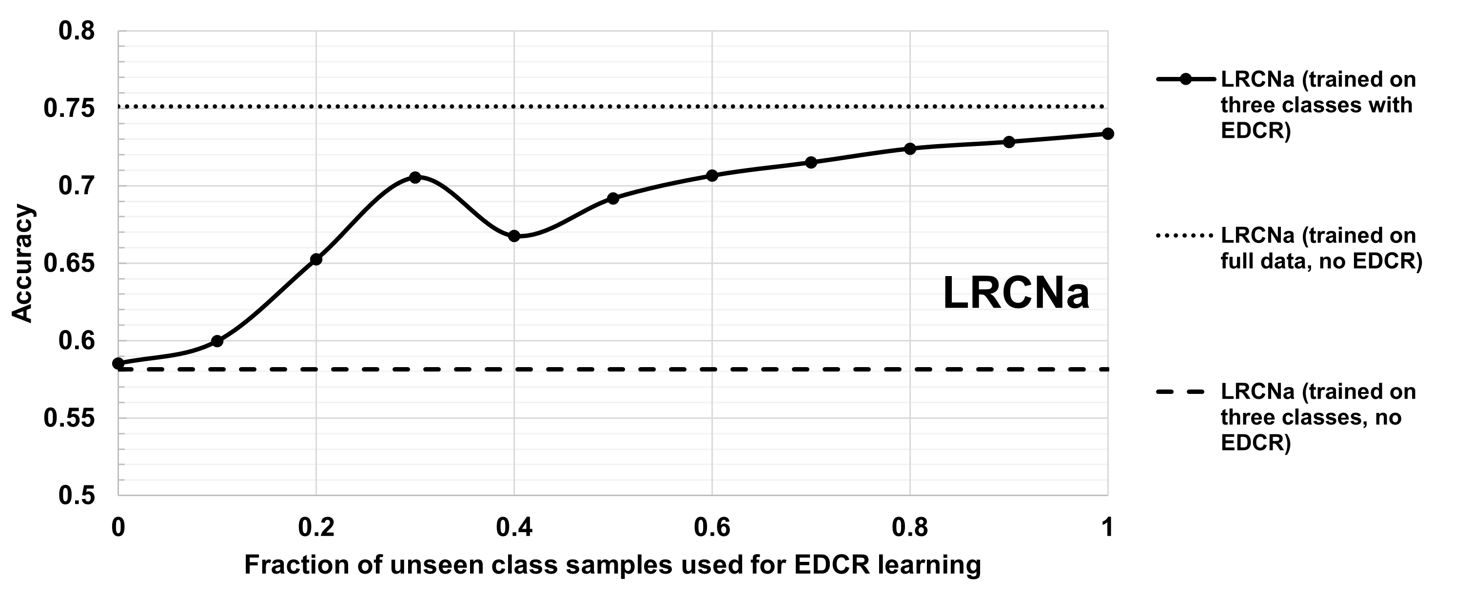
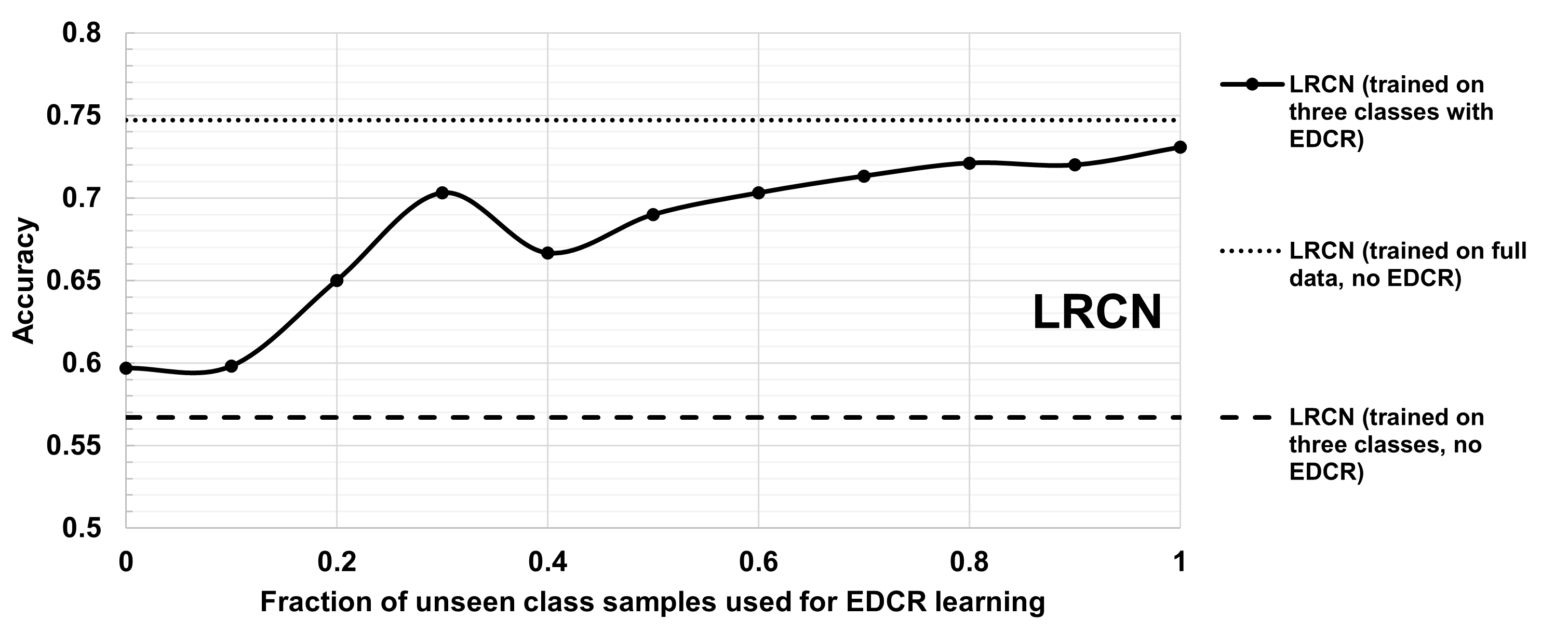
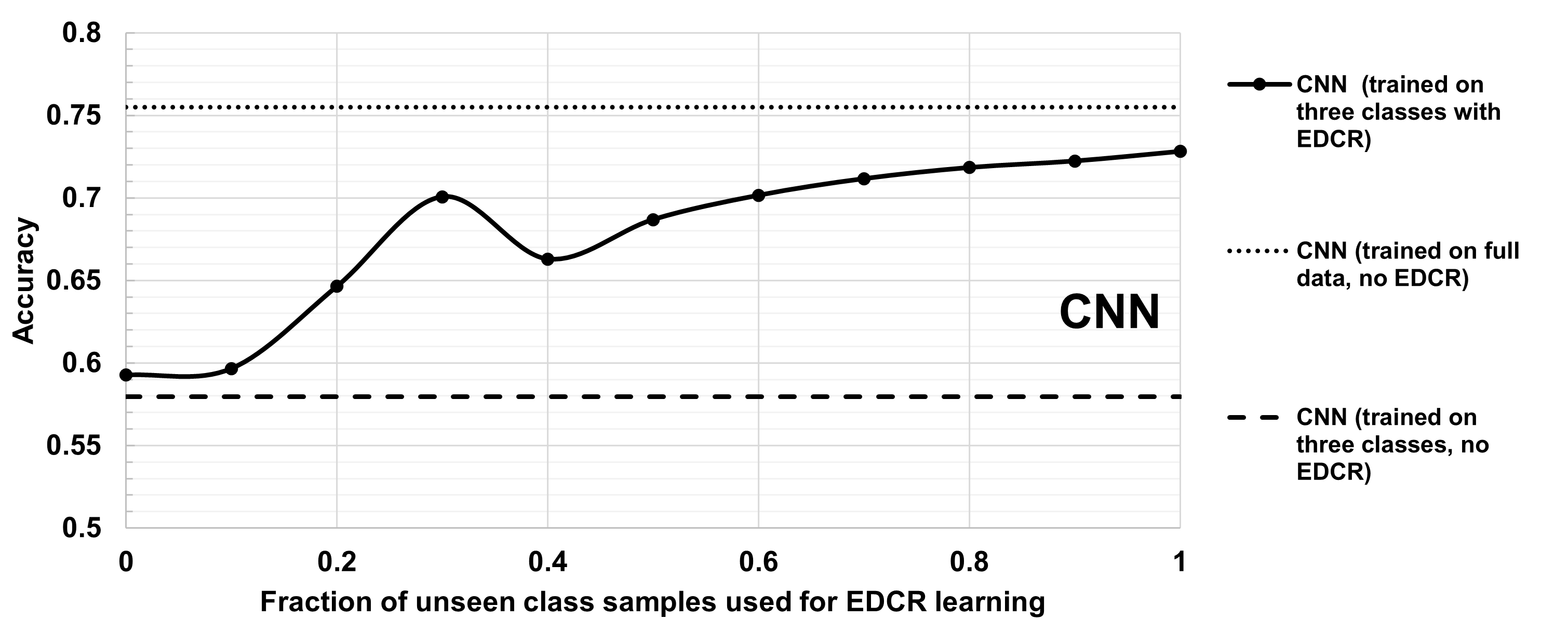
Figure 3: Results for experiments with two movement classes removed from training.

Appendix A Appendix

Details on Vector Embedding of Sequences

We begin with a set of GPS points where each point is a tuple of timestamp ($t$), latitude ($lat$), and longitude ($long$), $P_{i}=(t_{i},P^{lat}_{i},P^{long}_{i})$. Each point $P_{i}$ also has an associated class label $c\in\mathcal{C}$. To embed these tuples as vector embeddings that can be consumed by the neural model $f_{\theta}$, three essential preprocessing steps must be performed. These steps include normalizing the data size to meet the input requirements, extracting movement behaviors from the GPS points, and refining the data. In this section, we draw upon previous approaches (Zheng et al., 2008a,b; Dabiri et al., 2018; Kim, 2022) to guide the data preprocessing process.

As part of the data size normalization step we sequentially group chronologically ordered GPS points into uniform lengths of $40$. The class label $c$ of every point in this sequence is the same and the entire sequence represents the movement trajectory of that class for $40$ time units. The resulting sequence $\omega\in S$, where $S$ is the set of all sequences that are curated.

To capture patterns of movement behaviors from GPS points the distance time-series vector is computed as follows. $D^{j}_{i}$ is the distance between two GPS point tuples $P^{j}_{i}$ and $P^{j}_{i-1}$, where $j\in S$ and $i\in\omega$, and is computed using the Vincenty Distance formula  (Vincenty 1975). Here $D^{3}_{10}$ represents the distance between two points $P_{10}$ and $P_{9}$ from the $3^{rd}$ sequence. There could be cases where a distance time-series vector falls short of $40$ data points. To maintain a consistent length of sequence $\omega$ we pad the shorter $D^{j}$ vector with zeros.

Additionally, we extract the velocity ($V$), acceleration ($A$), jerk ($J$) and bearing rate ($BR$) time-series vectors for each sequence as follows:

$$V^{j}_{i}=\frac{\operatorname{Vincenty}\left(P^{j}_{i-1},P^{j}_{i}\right)}{t_{i}-t_{i-1}}$$ (1)

$$A^{j}_{i}=\frac{V^{j}_{i}-V^{j}_{i-1}}{t_{i}-t_{i-1}}$$ (2)

$$J^{j}_{i}=\frac{A^{j}_{i}-A^{j}_{i-1}}{t_{i}-t_{i-1}}$$ (3)

$$BR^{j}_{i}=\mid\text{ Bearing }_{i}-\text{ Bearing }_{i-1}\mid$$ (4)

$$\text{ where Bearing }_{i}=\arctan(y,x)$$ (5)

$$y=\sin\left(P_{i}^{\text{long }}-P_{i-1}^{\text{long }}\right)^{*}\cos\left(P_{i}^{\text{lat }}\right)$$ (6)

$$x=\cos\left(P_{i-1}^{\text{lat }}\right)*\sin\left(P_{i}^{\text{lat }}\right)-\sin\left(P_{i-1}^{\text{lat }}\right)*$$ (7)

$$\cos\left(P_{i}^{\text{lat }}\right)*\cos\left(P_{i}^{\text{long }}-P_{i-1}^{\text{long }}\right)$$

We finally stack the vectors $V^{j}$, $A^{j}$, $J^{j}$ and $BR^{j}$ for each sequence $\omega$, which is passed as the input to the neural model $f_{\theta}$ as detailed in section 2.

Formal Statements of Additional Theorems Corollaries for Error Detection Rules

Corollary 1.

If and only if $c\geq 1-P_{i}$ then the rule will cause precision not to decrease.

Corollary 2.

If $P_{i}\geq 1-c$ (the minimum condition for precision improvement from Corollary 1 then recall decreases by at most $s_{i}R_{i}$.

Theorem 4.

For a given error detecting rule, the quantity $c\cdot s_{i}$ is a normalized polymatroid function w.r.t. set $DC$.

Corollary 3.

The quantity $(1-c)s_{i}\frac{R_{i}}{R_{i}}$ (decrease in recall) is a normalized polymatroid function w.r.t. set $DC$.

Corollary 4.

GreedyRuleSelect provides an approximation of $cs$ that is within $1/|C|$ of optimal.

Formal Statements of Additional Theorems Corollaries for Error Correction Rules

Corollary 5.

Precision increases for class $i$ with the application of an error correcting rule if and only if $c>P_{i}$.

Corollary 6.

Recall is non-decreasing for class $i$ with the application of an error correcting rule.

Theorem 5.

Confidence is submodular with respect to $CC_{i}$.

Corollary 7.

For an arbitrarily small constant $\epsilon$, DetUSMPosRuleSelect provides a $1/3+\epsilon$ approximation of confidence if the returned confidence is greater than the initial precision.

Proof of Theorem 1

Under the condition $s_{i}\leq 1-P_{i}$, the precision of model $f_{\theta}$ for class $i$, with initial precision $P_{i}$, after applying an error correcting rule with support $s_{i}$ and confidence $c$ increases by a function of $s_{i}$ and $c$ and is greater than or equal to $c\cdot s_{i}$.

Proof.

CLAIM 1: The precision of model $f_{\theta}$ for class $i$, with initial precision $P_{i}$, after applying an error correcting rule with support $s_{i}$ and confidence $c$ increases by:

$$\frac{s_{i}}{1-s_{i}}(c+P_{i}-1)$$ (8)

The total number of items that $f_{\theta}$ will attempt to classify as $i$ before error correction is $N_{i}=TP_{i}+FP_{i}$. Out of those, $s_{i}\cdot N_{i}$ will be corrected by the rule. However, a fraction of $(1-c)$ will be samples that would have been true positives if not corrected. Hence, the new precision can be written as follows:

$$\frac{TP_{i}-(1-c)s_{i}\cdot N_{i}}{N_{i}-s_{i}\cdot N_{i}}$$ (9)

As $P_{i}\cdot N_{i}=TP_{i}$, we have:

$$\frac{P_{i}\cdot N_{i}-(1-c)s_{i}\cdot N_{i}}{N_{i}(1-s_{i})}$$ (10)

$$=\frac{P_{i}-(1-c)s_{i}}{(1-s_{i})}$$ (11)

Now we subtract from that quantity the initial precision.

$$\frac{P_{i}-(1-c)s_{i}}{(1-s_{i})}-P_{i}$$ (12)

$$=\frac{P_{i}-(1-c)s_{i}}{(1-s_{i})}-]\frac{(1-s_{i})P_{i}}{1-s_{i}}$$ (13)

$$=\frac{-s_{i}+s_{i}c+P_{i}s_{i}}{1-s_{i}}$$ (14)

$$=\frac{s_{i}}{1-s_{i}}(c+P_{i}-1)$$ (15)

CLAIM 2: If $s_{i}\leq 1-P_{i}$ then then $c\cdot s_{i}$ is a lower bound on the improvement in precision.

BWOC, then by Claim 1 we have.

$$\frac{s_{i}}{1-s_{i}}(c+P_{i}-1)>c\cdot s_{i}$$ (16)

$$c+P_{i}-1>c(1-s_{i})$$ (17)

$$c+P_{i}-1>c-c\cdot s_{i}$$ (18)

$$c\cdot s_{i}>1-P_{i}$$ (19)

$$c\cdot s_{i}>s_{i}$$ (20)

However, as $c\leq 1$ this is a contradiction.

The proof of the theorem then follows directly from claim 2. ∎

Proof of Corollarly 1

If and only if $c\geq 1-P_{i}$ then the rule will cause precision not to decrease.

Proof.

Suppose, BWOC, the statement is false. By Theorem 1 then the following must be true.

$$\frac{P_{i}-s_{i}(1-c)}{1-s_{i}}-P_{i}<0$$ (21)

$$P_{i}-s_{i}(1-c)<P(1-s_{i})$$ (22)

$$s_{i}c-s_{i}<-P_{i}s_{i}$$ (23)

$$P_{i}<1-c$$ (24)

However, as $P_{i}\geq 1-c$ this cannot hold.

Likewise, suppose BWOC that $c<1-P_{i}$ and BWOC the statement is false:

$$\frac{P_{i}-s_{i}(1-c)}{1-s_{i}}-P_{i}>0$$ (25)

$$P_{i}-s_{i}(1-c)>P(1-s_{i})$$ (26)

$$s_{i}c-s_{i}>-P_{i}s_{i}$$ (27)

$$P_{i}>1-c$$ (28)

Again, a contradiction. ∎

Proof of Theorem 4

For a given error detecting rule, the quantity $c\cdot s_{i}$ is a normalized polymatroid function w.r.t. set $DC$.

Proof.

CLAIM 1: $c\cdot s_{i}=POS/N_{i}$ where $POS$ is the number of samples where both the rule body and head are satisfied.
Let $BOD$ be the number of samples that the body of the rule is true. This gives us $c\cdot s_{i}=\frac{POS}{BOD}\frac{BOD}{N_{i}}$ which is equivalent to the statement of the claim. CLAIM 2: The quantity $c\cdot s_{i}$ is submodular w.r.t. set $DC$.
We show this by the subodularitiy of $POS$ as $N_{i}$ is a constant as well as the result of Claim 1. BWOC, $POS$ is not submodular for some set $DC$. We use the symbol $POS(DC)$ to denote this and assume the exsitence of two sets of conditions $DC_{1},DC_{2}$. Then, the following must be true:

$$POS(DC_{1})+POS(DC_{2})<POS(DC_{1}\cup DC_{2})$$ (29)

Which can be re-written as:

$$|\bigcup_{cond\in DC_{1}}\{x|cond(\omega)\wedge pred(\omega)\}|+$$ (30)

$$|\bigcup_{cond\in DC_{2}}\{x|cond(\omega)\wedge pred(\omega)\}|$$ (31)

This quantity is less than the following:

$$|\bigcup_{cond\in DC_{1}\cup DC_{2}}\{x|cond(\omega)\wedge pred_{x}\}|$$ (32)

However, this would imply there is at least one element in $DC_{1}\cup DC_{2}$ not in either $DC_{1}$ or $DC_{2}$ which is a contradiction. CLAIM 3: $c\cdot s_{i}$ monotonically increases with $DC$.
By claim 1, as the quantity equals $POS/N_{i}$ and $N_{i}$ is a constant, we just need to show monotonicity of $POS$. Clearly $POS$ increases monotonically as additional elements in $DC$ can only make it increase. CLAIM 4: When $DC=\emptyset$, $c\cdot s_{i}=0$.
Follows directly from the fact that we define $s_{i}$ as zero is no conditions are used.

Proof of theorem. Follows directly from claims 2-4. ∎

Proof of Theorem 2

After applying the rule to correct errors, the recall will decrease by

$$(1-c)s_{i}\frac{R_{i}}{P_{i}}$$ (33)

Proof.

The number of corrections made by the rule is $s_{i}(TP_{i}+FP_{i})$ with $(1-c)$ fraction of these being incorrect (increasing false negatives). Note that the sum $TP_{i}+FN$ does not change after error correction, as any “corrected” false positive becomes a false negative, and false negatives do not otherwise change from error correction. Therefore, the new recall is:

$$\frac{TP_{i}-s(1-c)(TP_{i}+FP_{i})}{TP_{i}+FN_{i}}$$ (34)

When this quantity is subtracted from the original recall ($R_{i}$), we obtain:

$$s_{i}(1-c)\left(R_{i}+\frac{FP_{i}}{TP_{i}+FN_{i}}\right)$$ (35)

We note that $FP_{i}=\frac{TP_{i}}{P_{i}}-TP_{i}=\frac{TP_{i}-P\cdot TP_{i}}{P_{i}}$ which gives us:

$$s_{i}(1-c)\left(R_{i}+\frac{TP_{i}}{P(TP_{i}+FN_{i})}-\frac{TP_{i}\cdot P_{i}}{P_{i}(TP_{i}+FN_{i})}\right)$$ (37)

$$=s_{i}(1-c)\left(R_{i}+\frac{R_{i}}{P_{i}}-R_{i}\right)$$ (38)

$$=(1-c)s_{i}\frac{R_{i}}{P_{i}}$$ (39)

∎

Proof of Corollary 2

If $P_{i}\geq 1-c$ (the minimum condition for precision improvement from Corollary 1 then recall decreases by at most $s_{i}R_{i}$.

Proof.

Suppose BWOC the statement is false. By Theorem 2, recall decrease by $(1-c)s_{i}\frac{R_{i}}{P_{i}}$. This gives us:

$$(1-c)s_{i}\frac{R_{i}}{P_{i}}>s_{i}R_{i}$$ (40)

Precision cannot be less than $1-c$, so recall must then decrease by:

$$(1-c)s_{i}\frac{R_{i}}{1-c}>s_{i}R_{i}$$ (41)

$$s_{i}R_{i}>s_{i}R_{i}$$ (42)

∎

Proof of Corollary 3

The quantity $(1-c)s_{i}\frac{R_{i}}{R_{i}}$ (decrease in recall) is a normalized polymatroid function w.r.t. set $DC$.

Proof.

Note that $BOD$ is the number of samples that satisfy the body, while $POS$ is the number of samples that satisfy the body and head, $NEG=POS-BOD$.

$$(1-c)s_{i}\frac{R_{i}}{P_{i}i}= \left(1-\frac{POS}{BOD}\right)\frac{BOD}{N_{i}}\frac{R_{i}}{P_{i}}$$ (43)

$$= \frac{NEG}{BOD}\frac{BOD}{N}\frac{R_{i}}{P_{i}}$$ (44)

$$= NEG\frac{1}{N_{i}}\frac{R_{i}}{P_{i}}$$ (45)

As $\frac{1}{N_{i}}\frac{R_{i}}{P_{i}}$ is a constant, we need to show the submodularity of $NEG$ which follows the same argument for $POS$ as per Claim 2 of Theorem 4. Likewise, $NEG$ is montonic (mirroring the argument of Claim 3 of Theorem 4) and normalized by the defintion of $s_{i}$ in the case where there are no conditions. The statement of the theorem follows. ∎

Proof of Theorem 3

For application of positive rules, precision increases if and only if rule confidence ($c$) increases.

Proof.

CLAIM 1: Precision increases by $\frac{cs-P_{i}s}{\mathbf{\mathcal{P}}_{i}+s}$.

The new precision is equal to the following:

$$\frac{TP_{i}+csN}{M_{i}+sN}$$ (46)

The improvement of the precision can be derived as follows.

$$\frac{TP_{i}+csN}{M_{i}+sN}-P_{i}=$$ (47)

$$= \frac{TP_{i}+csN-P_{i}M_{i}-P_{i}sN}{M_{i}+sN}$$ (48)

$$= \frac{TP_{i}+csN-TP_{i}-P_{i}sN}{M_{i}+sN}$$ (49)

$$= \frac{csN-P_{i}sN}{M_{i}+sN}$$ (50)

$$= \frac{cs-P_{i}s}{\mathbf{\mathcal{P}}_{i}+s}$$ (51)

CLAIM 2: If count of samples satisfying both rule body and head (the numerator of confidence) increases, then precision increases.

Suppose BWOC the claim is not true. Then for some value of $POS$ for which the improvement in precision is greater than $POS^{\prime}=POS+1$. Note that, in this case, the number of samples satisfying the body also increases by $1$. First, we know that we can re-write the result of claim 1 as follows.

$$\frac{POS-P_{i}BOD}{M_{i}+BOD}$$ (52)

Therefore, using the result from Claim 1, the following relationship must hold.

$$\frac{POS-P_{i}BOD}{M_{i}+BOD}>\frac{POS+1-P_{i}BOD-P_{i}}{M_{i}+BOD+1}$$ (53)

$$POS-P_{i}BOD>M_{i}(1-P_{i})+BOD(1-P_{i})$$ (54)

$$POS>M(1-P_{i})+BOD$$ (55)

This gives us a contradiction, as $M(1-P_{i})\geq 0$ and $POS\leq BOD$ by definition.

CLAIM 3: If the difference in precision increases, the number of samples satisfying both rule body and head must increase.
By definition, the only way for this to occur is if $BOD$ increases and $POS$ does not - as they can both increase or only $BOD$ increase. If neither there is no change, and it is not possible for $POS$ to increase without $BOD$. Therefore the following must be true.

$$\frac{POS-P_{i}BOD}{M_{i}+BOD}<\frac{POS-P_{i}BOD-P_{i}}{M_{i}+BOD+1}$$ (56)

However, this is clearly a contradiction the expression on the right is clearly smaller (the numerator is smaller as $P_{i}$ is positive, and the denominator is larger).

CLAIM 4: Precision increases if and only if $c$ increases.

Follows directly from claims 1-3.

CLAIM 5: When adding more samples that satisfy the body of the rule, confidence increases if and only if $POS$ increases.

Note that confidence is defined as $POS/BOD$. Clearly, there confidence decreases if $BOD$ increases but not $POS$ and it is not possible for $POS$ to increase alone. Therefore, BWOC, the following must hold true.

$$\frac{POS+k}{BOD+k}<\frac{POS}{BOD}$$ (57)

$$BODk<POSk$$ (58)

$$BOD<POS$$ (59)

This is a contradiction as $BOD\geq POS$.

Going other way, suppose BWOC confidence increases but POS does not. We get:

$$c_{2}>c_{1}$$ (60)

$$\frac{POS}{BOD_{2}}>\frac{POS}{BOD_{1}}$$ (61)

$$BOD_{1}>BOD_{2}$$ (62)

However, by the statement, as we add more samples that satisfy the body of the rule, we must have $BOD_{1}\leq BOD_{2}$. Hence a cotnradiction.

CLAIM 6: Recall increases if and only if $POS$ increases.

As we can write the new recall in this case simply as the following, the claim immediately follows.

$$\frac{TP_{i}+POS}{TP_{i}+FN_{i}}$$ (63)

CLAIM 7: Recall increases if and only if $c$ increases.

Follows directly from claims 5-6.

Proof of theorem.

Follows directly from claims 4 and 7. ∎

Proof of Theorem 5

Confidence is submodular with respect to $CC_{i}$.

Proof.

From claim 2 of Theorem 4 we showed $POS$ is submodular. The same proof can shwo quantity $BOD$ is submodular as well. We will use the symbol $BOD_{CC},POS_{CC}$ to denote $POS$ and $BOD$ with respect to set $CC$. BWOC assume confidence ($POS/BOD$) is not submodular. In what follows, we assume $C_{1}\subseteq C_{2}$. Therefore we get:

$$\frac{POS_{CC_{1}}}{BOD_{CC_{1}}}+\frac{POS_{CC_{2}}}{BOD_{CC_{2}}}<\frac{POS_{CC_{1}\cup CC_{2}}}{BOD_{CC_{1}\cup CC_{2}}}$$ (64)

$$\frac{POS_{CC_{1}}}{BOD_{CC_{2}}}+\frac{POS_{CC_{2}}}{BOD_{CC_{2}}}<\frac{POS_{CC_{1}\cup CC_{2}}}{BOD_{CC_{1}\cup CC_{2}}}$$ (65)

$$\frac{POS_{CC_{1}\cup CC_{2}}}{BOD_{CC_{2}}}<\frac{POS_{CC_{1}\cup CC_{2}}}{BOD_{CC_{1}\cup CC_{2}}}$$ (66)

$$BOD_{CC_{1}\cup CC_{2}}<BOD_{CC_{2}}$$ (67)

However, this is clearly a contradiction, completing the proof. ∎

Proof of Corollary 4

GreedyRuleSelect provides an approximation of $cs$ that is within $1/|C|$ of optimal.

Proof.

Follows directly from Theorem 4.7 of (Iyer and Bilmes 2013). ∎

Proof of Corollary 7

For an arbitrarily small constant $\epsilon$, DetUSMPosRuleSelect provides a $1/3+\epsilon$ approximation of confidence if the returned confidence is greater than the initial precision.

Proof.

Follows directly from the fact that confidence is zero when $CC_{i}=\emptyset$ and Theorem 2.3 of (Buchbinder et al. 2012). ∎

Conditions for Error Detection and Correction

In this section, we describe the various methods we used to create conditions (set $C$) in detail with examples.

Domain knowledge. Leveraging domain knowledge pertaining to outliers, we focused on the maximum velocity values present in our dataset. Notably, the highest speed records were associated with the drive labels. To ensure fair and consistent comparisons across the dataset, we conducted data normalization based on the maximum speed observed in the drive data. The highest velocity recorded in our dataset is 1, associated with the label drive.” Following closely is the train label, exhibiting a maximum velocity of 0.751.

In our datasets, any sample with a speed exceeding the maximum speed recorded for the train (0.751 in our dataset) is unambiguously classified as a drive. In a broader context, we apply the following condition: For instance, if a sample’s maximum speed measures 0.73—falling below both the maximum speeds of 0.751 attributed to the train class and 1 associated with the drive class, yet surpassing those of other categories—it indicates that the sample is likely to be categorized as either drive or train. we proceed to assess its multiclass prediction values. The class with the higher prediction value will ultimately determine our final classification for the sample.

Model based. In this study, we employed multiple models, denoted as $M$, each corresponding to a specific class. These models were constructed using our LRCNa architecture, as detailed in this paper. However, during the training process, we adapted the model $M$ to perform binary class classification. To illustrate, for the drive class, we divided the training data $\mathcal{T}$ into two distinct datasets: one exclusively containing samples labeled as drive, and the other encompassing samples labeled as walk, bike, bus, train, collectively forming the non_drive class. We employ this binary class classification approach to establish a set of conditions C.

References

- Aditya et al. (2023) Aditya, D.; Mukherji, K.; Balasubramanian, S.; Chaudhary, A.; and Shakarian, P. 2023. PyReason: Software for Open World Temporal Logic. In AAAI Spring Symposium.
- Buchbinder et al. (2012) Buchbinder, N.; Feldman, M.; Naor, J.; and Schwartz, R. 2012. A Tight Linear Time (1/2)-Approximation for Unconstrained Submodular Maximization. In 2012 IEEE 53rd Annual Symposium on Foundations of Computer Science, 649–658.
- Chen et al. (2021) Chen, L.; Lu, K.; Rajeswaran, A.; Lee, K.; Grover, A.; Laskin, M.; Abbeel, P.; Srinivas, A.; and Mordatch, I. 2021. Decision Transformer: Reinforcement Learning via Sequence Modeling. CoRR, abs/2106.01345.
- Dabiri and Heaslip (2018) Dabiri, S.; and Heaslip, K. 2018. Inferring transportation modes from GPS trajectories using a convolutional neural network. Transportation research part C: emerging technologies, 86: 360–371.
- Daftry et al. (2016) Daftry, S.; Zeng, S.; Bagnell, J. A.; and Hebert, M. 2016. Introspective Perception: Learning to Predict Failures in Vision Systems. .
- Fikioris et al. (2023) Fikioris, G.; Patroumpas, K.; Artikis, A.; Pitsikalis, M.; and Paliouras, G. 2023. Optimizing vessel trajectory compression for maritime situational awareness. GeoInformatica, 27(3): 565–591.
- Hospedales et al. (2021) Hospedales, T.; Antoniou, A.; Micaelli, P.; and Storkey, A. 2021. Meta-learning in neural networks: A survey. IEEE transactions on pattern analysis and machine intelligence, 44(9): 5149–5169.
- Huang, Cheng, and Weibel (2019) Huang, H.; Cheng, Y.; and Weibel, R. 2019. Transport mode detection based on mobile phone network data: A systematic review. Transportation Research Part C: Emerging Technologies, 101: 297–312.
- Itkina and Kochenderfer (2022) Itkina, M.; and Kochenderfer, M. J. 2022. Interpretable Self-Aware Neural Networks for Robust Trajectory Prediction. arXiv:2211.08701.
- Ivanov et al. (2021) Ivanov, R.; Carpenter, T.; Weimer, J.; Alur, R.; Pappas, G.; and Lee, I. 2021. Verisig 2.0: Verification of Neural Network Controllers Using Taylor Model Preconditioning. In Computer Aided Verification: 33rd International Conference, CAV 2021, Virtual Event, July 20–23, 2021, Proceedings, Part I, 249–262. Springer-Verlag. ISBN 978-3-030-81684-1.
- Iyer and Bilmes (2013) Iyer, R.; and Bilmes, J. 2013. Submodular Optimization with Submodular Cover and Submodular Knapsack Constraints. In Proceedings of the 26th International Conference on Neural Information Processing Systems - Volume 2, NIPS’13, 2436–2444. Red Hook, NY, USA: Curran Associates Inc.
- Janner, Li, and Levine (2021) Janner, M.; Li, Q.; and Levine, S. 2021. Offline Reinforcement Learning as One Big Sequence Modeling Problem. In Advances in Neural Information Processing Systems.
- Jothimurugan et al. (2021) Jothimurugan, K.; Bansal, S.; Bastani, O.; and Alur, R. 2021. Compositional Reinforcement Learning from Logical Specifications. In Advances in Neural Information Processing Systems.
- Kim, Kim, and Lee (2022) Kim, J.; Kim, J. H.; and Lee, G. 2022. GPS data-based mobility mode inference model using long-term recurrent convolutional networks. Transportation Research Part C: Emerging Technologies, 135: 103523.
- Lin and Hsu (2014) Lin, M.; and Hsu, W.-J. 2014. Mining GPS data for mobility patterns: A survey. Pervasive and mobile computing, 12: 1–16.
- Ma et al. (2020) Ma, M.; Gao, J.; Feng, L.; and Stankovic, J. 2020. STLnet: Signal temporal logic enforced multivariate recurrent neural networks. Advances in Neural Information Processing Systems, 33: 14604–14614.
- Ramanagopal et al. (2018) Ramanagopal, M. S.; Anderson, C.; Vasudevan, R.; and Johnson-Roberson, M. 2018. Failing to Learn: Autonomously Identifying Perception Failures for Self-driving Cars. 3(4): 3860–3867.
- Simoncini et al. (2018) Simoncini, M.; Taccari, L.; Sambo, F.; Bravi, L.; Salti, S.; and Lori, A. 2018. Vehicle classification from low-frequency GPS data with recurrent neural networks. Transportation Research Part C: Emerging Technologies, 91: 176–191.
- Vanschoren (2018) Vanschoren, J. 2018. Meta-learning: A survey. arXiv preprint arXiv:1810.03548.
- Vaswani et al. (2017) Vaswani, A.; Shazeer, N.; Parmar, N.; Uszkoreit, J.; Jones, L.; Gomez, A. N.; Kaiser, Ł.; and Polosukhin, I. 2017. Attention is all you need. In Advances in Neural Information Processing Systems, 5998–6008.
- Vincenty (1975) Vincenty, T. 1975. Direct and inverse solutions of geodesics on the ellipsoid with application of nested equations. Survey review, 23(176): 88–93.
- Wang et al. (2017) Wang, H.; Liu, G.; Duan, J.; and Zhang, L. 2017. Detecting transportation modes using deep neural network. IEICE TRANSACTIONS on Information and Systems, 100(5): 1132–1135.
- Zeng et al. (2023) Zeng, J.; Yu, Y.; Chen, Y.; Yang, D.; Zhang, L.; and Wang, D. 2023. Trajectory-as-a-Sequence: A novel travel mode identification framework. 146: 103957.
- Zheng et al. (2008) Zheng, Y.; Li, Q.; Chen, Y.; Xie, X.; and Ma, W.-Y. 2008. Understanding mobility based on GPS data. In Proceedings of the 10th international conference on Ubiquitous computing, 312–321.
- Zhou et al. (2022) Zhou, K.; Liu, Z.; Qiao, Y.; Xiang, T.; and Loy, C. C. 2022. Domain generalization: A survey. IEEE Transactions on Pattern Analysis and Machine Intelligence.