Statistical Inference on Grayscale Images via the Euler-Radon Transform

Abstract

Tools from topological data analysis have been widely used to represent binary images in many scientific applications. Methods that aim to represent grayscale images (i.e., where pixel intensities instead take on continuous values) have been relatively underdeveloped. In this paper, we introduce the Euler-Radon transform, which generalizes the Euler characteristic transform to grayscale images by using o-minimal structures and Euler integration over definable functions. Coupling the Karhunen–Loève expansion with our proposed topological representation, we offer hypothesis-testing algorithms based on the $\chi^{2}$ distribution for detecting significant differences between two groups of grayscale images. We illustrate our framework via extensive numerical experiments and simulations.

1 Introduction

The analysis of grayscale images is important in many fields. In medical imaging, data can be derived from different modalities including magnetic resonance imaging (MRI), computed tomography (CT), positron emission tomography (PET), and micro-computed tomography (Micro-CT). Analyzing the variation among pixel intensities in these images can help diagnose diseases, detect abnormalities in human tissues, and monitor the effectiveness of different treatment strategies (e.g., see Figure 1). Beyond medicine, grayscale imaging is essential in astronomy for capturing details in celestial bodies and other phenomena (Howell, 2006), in geology for studying rock and mineral compositions using electron microscopy (Reed, 2005), and in meteorology for interpreting satellite imagery to predict weather patterns (Kidder and Haar, 1995).

There is an important distinction between binary and grayscale images. Unlike binary images, where pixels are exactly one of two colors (usually black and white), pixels in grayscale images take on continuous values. A binary image can be modeled as a binary-valued function which is often expressed in the following form

$$\mathbbm{1}_{K}(x)=\left\{\begin{aligned} 1,\ \ &\mbox{ if the color of point (pixel) $x$ is white},\\ 0,\ \ &\mbox{ if the color of point (pixel) $x$ is black},\end{aligned}\right.$$ (1.1)

where the subscript $K$ denotes the region of white points in the image (which we will refer to as a “shape” throughout this paper). In contrast, a grayscale image must be modeled as a real-valued function. Specifically, the grayscale intensity of each pixel is represented as the function value at that corresponding point.

Many methods in the field of topological data analysis (TDA) (Carlsson, 2009, Vishwanath et al., 2020) have been developed for analyzing binary images (equivalently, shapes). Some of these works include the persistent homology transform (PHT) (Turner et al., 2014), the Euler characteristic transform (ECT) (Turner et al., 2014, Ghrist et al., 2018), and the smooth Euler characteristic transform (SECT) (Crawford et al., 2020) — all of which are proposed statistics used to represent shapes while preserving the complete information they contain. Crawford et al. (2020) applied the SECT on MRI-derived binary images taken from tumors of glioblastoma multiforme (GBM) patients. Here, the authors used the resulting summary statistics from the SECT in a class of Gaussian process regression models to predict survival-based outcomes. Wang et al. (2021) utilized the ECT for sub-image analysis which aims to identify geometric features that are important for distinguishing various classes of shapes. Marsh et al. (2022) recently presented the DETECT: an extension of the ECT to analyze temporal changes in shapes. The authors demonstrated their approach by studying the growth of mouse small intestine organoid experiments from segmented videos. Lastly, Meng et al. (2022) recently used the SECT framework to introduce a $\chi^{2}$ distribution-based approach to test hypotheses on random shapes, with the corresponding mathematical foundation being established therein through algebraic topology, functional analysis with Sobolev embeddings (Brezis, 2011), and probability theory using the Karhunen–Loève expansion (Alexanderian, 2015).

Previous TDA methods that use Euler characteristic-based invariants are well suited for binary images and shapes with clearly defined boundaries (e.g., the region $K$ of white points defined via the binary-valued function in Eq. (1.1)). Grayscale images, on the other hand, are arrays of 2-dimensional pixel or 3-dimensional voxel intensities that represent varying levels of brightness in a continuous space (e.g., see Figures 1 and 2). These images lack the clear boundaries that can be used to define and compute the Euler characteristic. Consequently, due to the inherent continuous nature of grayscale images, both the Euler characteristic and the corresponding TDA methods that leverage it are not immediately applicable.

One natural way to apply the Euler characteristic to grayscale images is through binary image segmentation (BIS) — a process that divides points in a grayscale image into foreground (the shape of interest) and background. That is, BIS can serve as a preprocessing step to convert a grayscale image into a binary format, facilitating the application of the Euler characteristic. Numerous state-of-the-art applications of Euler characteristic-based TDA methods to grayscale images rely on BIS. For example, Crawford et al. (2020) used the computer-assisted program MITKats (Chen and Rabadán, 2017) to threshold MRI scans of GBM tumors and convert them to binary formats for their analyses with the SECT (refer to Figure 3 in Crawford et al. (2020)). Unfortunately, there are several challenges associated with BIS that can impede on the effectiveness and accuracy of downstream analyses with TDA methods. One of the primary challenges is selecting an appropriate threshold to distinguish between foreground and background points. Improper choice of a BIS threshold may result in the issue of over- or under-segmentation. Moreover, pinpointing a proper threshold is often not straightforward (especially when the images have low image contrast, large noise, or complex heterogeneity) and can be computationally demanding. This selection process can be especially challenging for medical images of soft tissues (including organs, tumors, and blood vessels). Most importantly, performing BIS inevitably causes a loss of information in images of interest. By generalizing Euler characteristic-based statistics and enabling them to be directly applicable to grayscale images without the need for BIS, we will increase their utility for better powered shape analyses.

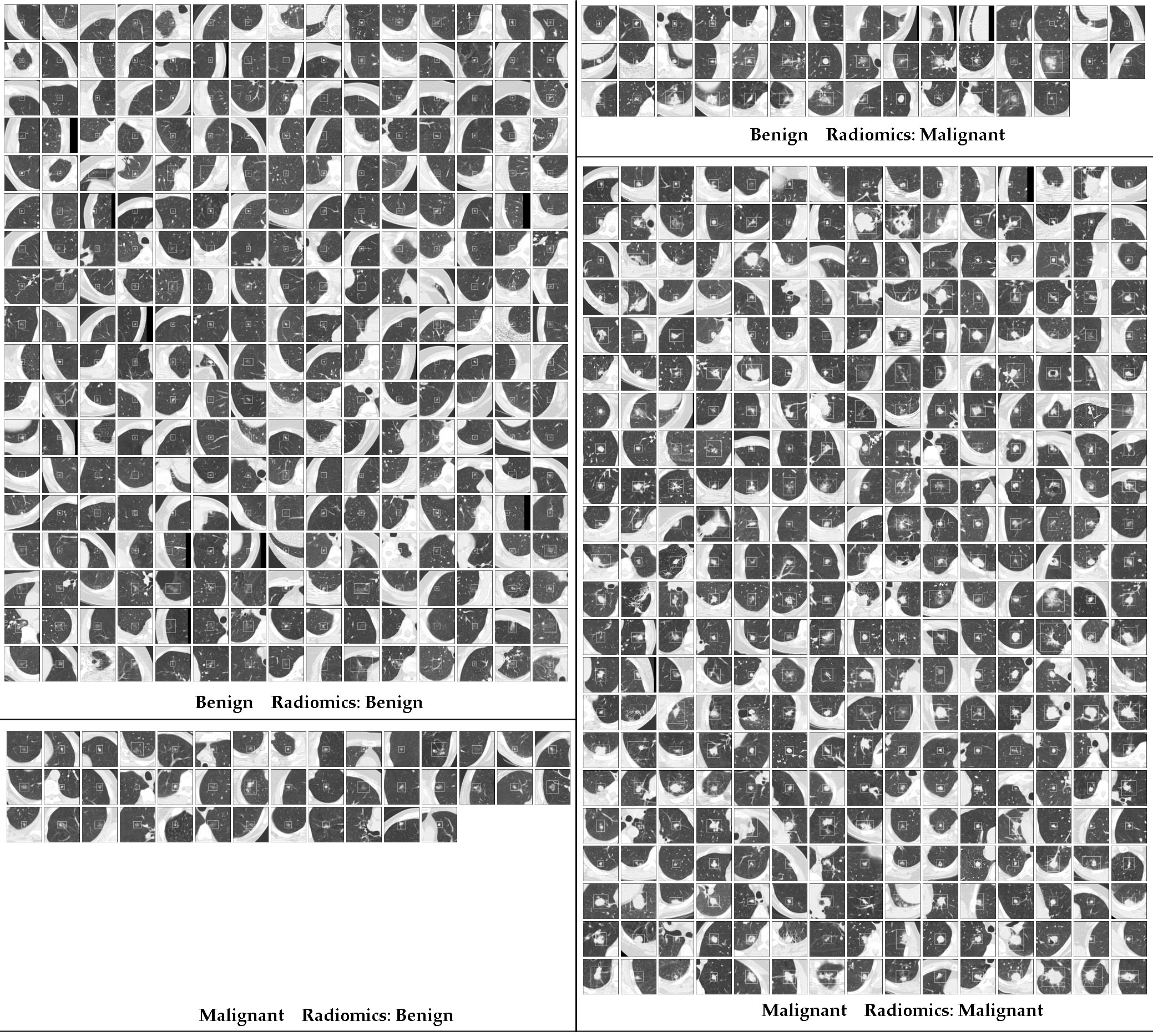
Figure 1: CT scans of lung cancer tumors labeled as “benign” or “malignant.” This figure has been previously published in Maldonado et al. (2021). The details of this figure are provided therein.

Radiomics (Aerts et al., 2014) has been used to estimate features from grayscale images to predict outcomes of interest, such as patient survival time in cancer. Most commonly used radiomics approaches are based on estimating parameters that describe various image intensity features, which are then employed for prediction. For example, Just (2014) described the estimation of moments of intensity histograms, Brooks and Grigsby (2013) proposed a pixel-based distance-dependent approach using the deviation from a linear intensity gradation, and Eloyan et al. (2020) described an approach for estimation of intensity histogram and shape features taking into account the correlation structure of pixel intensities. Additionally, Aerts et al. (2014) showed the computation of shape and texture features from the image intensities. While radiomic features computed from grayscale images can be used to compare populations of images, they also inevitably lose information about the grayscale images of interest. This loss reduces the power of downstream statistical analyses.

The major contributions that we present in this paper all center around developing a generalization of the ECT for grayscale images. A summary of these include:

1. Utilizing o-minimal structures (van den Dries, 1998) and the framework proposed in Baryshnikov and Ghrist (2010) for Euler integration over definable functions, we introduce the Euler-Radon transform (ERT). This ERT serves as a topological summary statistic that aims to unify the ECT (Turner et al., 2014, Ghrist et al., 2018), the weighted Euler curve transform (WECT) (Jiang et al., 2020), and the marginal Euler curve (MEC) (Kirveslahti and Mukherjee, 2023). Notably, when the ERT is employed on binary images, it coincides with the ECT. Moreover, akin to the framework presented in Kirveslahti and Mukherjee (2023), our ERT does not rely on the diffeomorphism assumption posited in many state-of-the-art methods (e.g., Ashburner, 2007). Lastly, unlike previous TDA-based methods that rely on BIS and standard radiomic approaches, the “Schapira inversion formula” (Schapira, 1995) guarantees that our proposed ERT summary preserves all information within the pixel intensity arrays of grayscale images.

2. Using the proposed ERT as a building block, we also introduce the smooth Euler-Radon transform (SERT). When applied to binary images, the SERT coincides with the SECT (Crawford et al., 2020, Meng et al., 2022). Importantly, the SERT represents the grayscale images as functional data. Numerous tools from functional data analysis (FDA) (Hsing and Eubank, 2015) and functional analysis (Brezis, 2011) are applicable with the SERT (e.g., the Karhunen–Loève expansion Alexanderian, 2015).

3. Using the ERT and SERT, we propose several statistical algorithms aimed at detecting significant differences between paired collections of grayscale images (e.g., analyzing CT scans of malignant and benign tumors from Figure 1). Particularly, our proposed algorithms combine the Karhunen–Loève expansion with a permutation-based approach. Using simulations, we show that our hypothesis test is uniformly powerful across various scenarios and does not suffer from type I error inflation. These algorithms are a generalization of results presented in Meng et al. (2022).

Beyond the contributions outlined above, due to the resemblance between the ECT and our proposed ERT, this paper paves the way for generalizing a series of ECT-based methods (Crawford et al., 2020, Wang et al., 2021, Marsh et al., 2022) from binary images to grayscale images.

The remainder of this paper is organized as follows. In Section 2, we review some existing representations of grayscale images. In Section 3, we first review the basics of Euler calculus that have been described in van den Dries (1998), Baryshnikov and Ghrist (2010), and Ghrist (2014). Then, using Euler calculus, we define the ERT and detail its properties. In Section 4, we comprehensively describe the relationship between our proposed ERT and existing topological representations of grayscale images (Jiang et al., 2020, Kirveslahti and Mukherjee, 2023). Section 5 offers a proof-of-concept example that illustrates the behavior of our proposed SERT. In Section 6, we propose an ERT-based alignment approach for preprocessing grayscale images prior to statistical inference without relying on correspondences between them. In Section 7, we propose several statistical algorithms designed to differentiate between two sets of grayscale images. The performance of the proposed algorithms is presented in Section 8 using simulations. Lastly, we conclude this paper in Section 9 and discuss several future research directions. The proofs of all theorems in this paper are provided in Appendix A unless otherwise stated.

2 Representations of Grayscale Images

The statistical inference on grayscale images necessitates an appropriate representation of grayscale images. For the application of statistical methods akin to the ECT-based methods in Crawford et al. (2020), Wang et al. (2021), Meng et al. (2022), and Marsh et al. (2022), it is imperative that our proposed representation of grayscale images aligns as closely as possible with the ECT. Prior to delving into our proposed approach, this section offers a review of some existing representations of grayscale images.

In an attempt to employ an ECT-like method to grayscale images of GBM tumors, Jiang et al. (2020) transformed each grayscale image into the discrete representation $\sum a_{\sigma}\cdot\mathbbm{1}_{\sigma}(x)$ in their preprocessing step, where $\sum$ denotes a finite sum, each $\sigma$ is a simplicial complex, and each weight $a_{\sigma}$ belongs to $\mathbb{N}:=\{0,1,2,\ldots\}$. In other words, each grayscale image is transformed into a weighted sum of a finite set of simplexes (referred to as a “weighted complex” therein). Subsequently, Jiang et al. (2020) introduced the weighted Euler curve transform (WECT) tailored for weighted complexes. A limitation of the WECT method is the dependency of data analysis results on the discretization $\sum a_{\sigma}\cdot\mathbbm{1}_{\sigma}(x)$, unless the original image is discrete and can be exactly depicted as a weighted complex. When dealing with a high-resolution grayscale image, the deviation between the original image and its weighted complex discretization can be substantial. Importantly, the reliance of data analysis on the discretization complicates theoretical analysis, which necessitates discretization-free representations of grayscale images.

Many state-of-the-art methods for analyzing grayscale images rely on the diffeomorphism assumption that the grayscale images being analyzed are diffeomorphic (e.g., Ashburner, 2007). To obviate the diffeomorphism assumption, Kirveslahti and Mukherjee (2023) introduced two novel representations called the lifted Euler characteristic transform (LECT) and the super LECT (SELECT) utilizing a lifting technique. In contrast to the approach proposed by Jiang et al. (2020), neither the LECT nor SELECT depends on the discretization preprocessing for grayscale images. However, the lifting procedure used in both the LECT and SELECT introduces an additional dimension. For example, the LECT represents a $d$-dimensional grayscale image as a function on a $(d+1)$-dimensional manifold (see Eq. (4.1) for details). This increase in dimensionality distinguishes the LECT and SELECT distinctly from the ECT, precluding straightforward theoretical and methodological generalizations of ECT-based methods to grayscale images (Ghrist et al., 2018, Crawford et al., 2020, Wang et al., 2021, Meng et al., 2022, Marsh et al., 2022). Additionally, the augmented dimensionality elevates the computational expense associated with subsequent statistical inference.

A grayscale image can also be represented using function values where $g(x)$ is used to denote the grayscale intensity at point (pixel) $x$. One straightforward approach to quantify differences between two images can then be done using the Lebesgue integral $\int|g^{(1)}(x)-g^{(2)}(x)|^{2}\,dx$ for grayscale images represented by functions $g^{(1)}$ and $g^{(2)}$. Representing grayscale images through topological invariants presents distinct advantages compared to using function values. These advantages have been documented by Kirveslahti and Mukherjee (2023). As a toy example, the Euler characteristic of a singular point is 1; whereas, its Lebesgue integral is 0.

3 Euler-Radon Transform of Grayscale Functions

In this section, we generalize the ECT from binary images to grayscale images via the Euler calculus (Baryshnikov and Ghrist, 2010, Ghrist, 2014). This generalization does not depend on the discretization of grayscale images nor does it introduce an additional dimension. More precisely, we introduce the Euler-Radon transform (ERT) as a means to perform statistical inference on grayscale images. This approach serves as a natural extension of both the ECT and WECT, and has a direct connection to the LECT and SELECT. Furthermore, to apply functional data analysis, we propose a smooth version of the ERT — the smooth Euler-Radon transform (SERT), which is a generalization of the SECT.

3.1 Outline

To elucidate the conceptual foundation of our ERT as an extension of the ECT, we revisit the ECT of shapes $K$ from the viewpoint of Euler calculus. The discussion in this subsection primarily serves a heuristic purpose; a thorough and precise exposition is given in Section 3.3.

Without loss of generality, we assume $K\subseteq B_{\mathbb{R}^{d}}(0,R):=\{x\in\mathbb{R}^{d}:\|x\|<R\}$ for a prespecified radius $R>0$ and $K$ is compact. The ECT of $K$ is a collection of Euler characteristics $\{\chi(K_{t}^{\nu}):\,(\nu,t)\in\mathbb{S}^{d-1}\times[0,2R]\}$, where $\chi\left(K_{t}^{\nu}\right)\text{ is the Euler characteristic of }K_{t}^{\nu}$ and $K_{t}^{\nu}:=\{x\in K:\,x\cdot\nu\leq t-R\}$ (also Meng et al., 2022). The Euler characteristic $\chi\left(K_{t}^{\nu}\right)$ can be represented as follows using the Euler functional $\int(\cdot)d\chi$ (e.g., Ghrist et al., 2018)

$$\begin{aligned} &\chi\left(K_{t}^{\nu}\right)=\int\mathbbm{1}_{K}(x)\cdot R(x,\nu,t)\,d\chi(x),\\ &\text{where }\ \ R(x,\nu,t):=\mathbbm{1}\left\{\left(x,\nu,t\right)\in B_{\mathbb{R}^{d}}(0,R)\times\mathbb{S}^{d-1}\times[0,T]\,:\,x\cdot\nu\leq t-R\right\}\text{ and }T:=2R.\end{aligned}$$ (3.1)

In essence, this formulation can be viewed as a generalized Radon transform of the function $\mathbbm{1}_{K}$ (Schapira, 1995, Baryshnikov et al., 2011, Ghrist et al., 2018). Here, the indicator function $\mathbbm{1}_{K}$ represents a binary image, as referenced in Eq. (1.1). In the development of the ERT, our primary objective is to substitute the indicator function $\mathbbm{1}_{K}$ in Eq. (3.1) with a real-valued function $g$ representing a grayscale image.

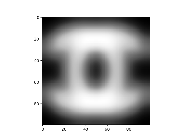
(a)

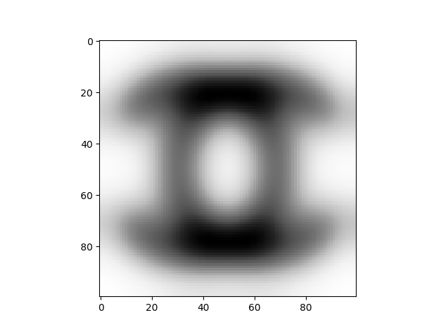
(b)

Figure 2: Panel (a) shows a grayscale image represented by a function $g$ in the form of Eq. (3.2). Here, each white pixel corresponds to value 1 and each black pixel corresponds to 0. Panel (b) presents a rescaled version of $g$, where the negative coefficient $\lambda$ induces a “white-to-black” transition. In this image, each white pixel corresponds to value 0 and each black pixel corresponds to value -0.5.

A conventional approach to modeling a grayscale image $g$ takes the form

$$g(x)=\left\{\begin{aligned} &1,\ \ \ \mbox{ if the color at point (pixel) $x$ is white},\\ &\#,\ \ \ \mbox{the value of the grayscale intensity at point (pixel) $x$ scaled between 0 and 1,}\\ &0,\ \ \ \mbox{ if the color at point (pixel) $x$ is black}.\end{aligned}\right.$$ (3.2)

For reference, we encourage readers to compare Eq. (3.2) with Eq. (1.1). An example of a grayscale image is presented in Figure 2(a). In many applications, it becomes important to rescale a grayscale image where $g(x)\mapsto\lambda\cdot g(x)$ for $\lambda\in\mathbb{R}$. However, the configuration in Eq. (3.2) is not invariant under this rescaling transform. Therefore, we will no longer view a grayscale image as a function taking values between $[0,1]$. Instead, throughout this paper, we will treat each grayscale image generally as a bounded function $g$, which we subsequently term a grayscale function (see Section 3.3 for details). Obviously, a rescaled bounded function is still bounded, although it may take values outside $[0,1]$. Furthermore, for negative $\lambda$, this rescaling inverts the grayscale spectrum, reminiscent of a “white-to-black” transition (an example of this is available in Figure 2(b)). By encompassing general bounded functions — beyond those merely within the $[0,1]$ range — our approach broadens its applicability, encapsulating scalar fields that are beyond the structure posited in Eq. (3.2) (e.g., the realizations of Gaussian random fields) (Adler et al., 2007, Bobrowski and Borman, 2012).

As previously mentioned, the key to generalizing the ECT to the ERT is replacing the indicator function $\mathbbm{1}_{K}$ in Eq. (3.1) with a real-valued function $g$ representing a grayscale image. That is, the ERT of a $d$-dimensional grayscale image $g$ can be heuristically expressed as follows

$$\int g(x)\cdot R(x,\nu,t)\,d\chi(x),$$ (3.3)

which is a function of $(\nu,t)$ on the $d$-dimensional manifold $\mathbb{S}^{d-1}\times[0,T]$. If the grayscale function $g$ in Eq. (3.3) takes only finitely many values in $\mathbb{Z}$ (e.g., $g$ is a discretized version of some underlying high-resolution grayscale image), the integration in Eq. (3.3) can be easily defined via the Euler integration over constructible functions (see Section 3.6 of Ghrist (2014)) and is equal to the WECT under some tameness conditions (Jiang et al., 2020). When the grayscale function $g$ has an “infinitely fine resolution” (i.e., $g$ is generally real-valued), the rigorous definition of the integration in Eq. (3.3) necessitates the techniques developed in Baryshnikov and Ghrist (2010). A more elaborate discussion on this, using o-minimal structures, will be discussed in Section 3.2.

3.2 Euler Calculus via O-minimal Structures

The primary objective of this subsection is to revisit Euler calculus — to prepare for a rigorous version of the heuristic integration presented in Eq. (3.3). This will result in the precise definition of the ERT which we detail in Section 3.3.

O-minimal Structures and Definable Functions.

Euler calculus has been extensively examined in the literature (Baryshnikov and Ghrist, 2010, Ghrist, 2014). Lebesgue integration is established for measurable functions. In a manner similar to Lebesgue integration, Euler integration begins by determining a set of functions that act as integrands for Euler integrals. These specific functions are termed “definable functions” and are specified through o-minimal structures. The definition of o-minimal structures is available in van den Dries (1998) and rephrased as follows:

Definition 3.1.

An o-minimal structure on $\mathbb{R}$ is a sequence $\mathcal{O}=\{\mathcal{O}_{n}\}_{n\geq 1}$ satisfying the following axioms:
(i) for each $n$, the collection $\mathcal{O}_{n}$ is a Boolean algebra of subsets of $\mathbb{R}^{n}$;
(ii) $A\in\mathcal{O}_{n}$ implies $A\times\mathbb{R}\in\mathcal{O}_{n+1}$ and $\mathbb{R}\times A\in\mathcal{O}_{n+1}$;
(iii) $\{(x_{1},\ldots,x_{n})\in\mathbb{R}^{n}\,:\,x_{i}=x_{j}\}\in\mathcal{O}_{n}$ for all $1\leq i<j\leq n$;
(iv) $A\in\mathcal{O}_{n+1}$ implies $\pi(A)\in\mathcal{O}_{n}$, where $\pi:\mathbb{R}^{n+1}\rightarrow\mathbb{R}^{n}$ is the projection map on the first $n$ coordinates;
(v) $\{r\}\in\mathcal{O}_{1}$ for all $r\in\mathbb{R}$, and $\{(x,y)\in\mathbb{R}^{2}\,:\,x<y\}\in\mathcal{O}_{2}$;
(vi) the only sets in $\mathcal{O}_{1}$ are the finite unions of open intervals (with $\pm\infty$ endpoints allowed) and points.
A set $K$ is said to be definable with respect to $\mathcal{O}$ if $K\in\mathcal{O}$ (i.e., there exists an $n$ such that $K\in\mathcal{O}_{n}$).

A typical example of o-minimal structures is the collection of semialgebraic sets which is defined as: a set $K\subseteq\mathbb{R}^{n}$ is said to be a semialgebraic subset of $\mathbb{R}^{n}$ if it is a finite union of sets of the following form

$$\Big{\{}x\in\mathbb{R}^{n}\,:\,p_{1}(x)=0,\,\ldots,\,p_{k}(x)=0,\,q_{1}(x)>0,\,\ldots,\,q_{l}(x)>0\Big{\}},$$

where $k$ and $l$ are positive integers, and $p_{1},\ldots,p_{k},q_{1},\ldots,q_{l}$ are real polynomial functions on $\mathbb{R}^{n}$ (also see Chapter 2 of van den Dries (1998)). Specifically, if we let $\mathcal{O}_{n}=$ the collection of semialgebraic subsets of $\mathbb{R}^{n}$, then $\mathcal{O}=\{\mathcal{O}_{n}\}_{n\geq 1}$ is an o-minimal structure. Since the unit sphere $\mathbb{S}^{n-1}=\{x\in\mathbb{R}^{n}:\,\|x\|^{2}-1=0\}$ is defined using the polynomial $\|x\|^{2}-1$, it is definable with respect to this o-minimal structure. It is also true for the open ball $B_{\mathbb{R}^{n}}(0,R)=\left\{x\in\mathbb{R}^{n}:\,\|x\|^{2}-R<0\right\}$ centered at the origin with radius $R>0$. Throughout this paper, to include many common sets in our framework, we assume the o-minimal structures $\mathcal{O}$ of interest to satisfy the following assumption:

Assumption 1.

The o-minimal structure $\mathcal{O}$ of interest contains all semialgebraic sets.

Importantly, under Assumption 1, we are able to apply the “triangulation theorem” and the “trivialization theorem” as presented in van den Dries (1998). In particular, the “triangulation theorem” (see Chapter 8 of van den Dries (1998)) indicates that each definable set is homeomorphic to a polyhedron, which subsequently suggests that each definable set is Borel-measurable (see “Definition 1.21” of Klenke (2020)).

In addition to o-minimal structures, we need the concepts in the following definition, which are also available in Baryshnikov and Ghrist (2010).

Definition 3.2.

Suppose we have an o-minimal structure $\mathcal{O}$ on $\mathbb{R}$. Let $X$ be definable and $Y\subseteq\mathbb{R}^{N}$ for some positive integer $N$.

1. A function $g:X\rightarrow Y$ is said to be definable if its graph $\Gamma(g):=\{(x,y)\in X\times Y:y=g(x)\}$ is definable (i.e., $\Gamma(g)\in\mathcal{O}$).

2. Let $\operatorname{Def}(X;Y)$ denote the collection of compactly supported definable functions $g:X\rightarrow Y$. Denote $\operatorname{Def}(X):=\operatorname{Def}(X;\mathbb{R})$.

3. Denote $\operatorname{CF}(X):=\operatorname{Def}(X;\,\mathbb{Z})$. Any function in $\operatorname{CF}(X)$ is called a constructible function.

4. If a definable set is also compact, we call this set a constructible set; the collection of all constructible subsets of $X$ is denoted by $\operatorname{CS}(X)$. Obviously, for any constructible subset $K\subseteq X$, $K\mapsto\mathbbm{1}_{K}$ is an injective map from $\operatorname{CS}(X)$ to $\operatorname{CF}(X)$.

It is simple to verify that, under Assumption 1, the function $R(x,\nu,t)$ defined in Eq. (3.1) is a constructible function where $R\in\operatorname{CF}(\mathbb{R}^{2d+1})$, and $\{(x,\nu,t)\in\mathbb{R}^{2d+1}\,:\,R(x,\nu,t)=1\}$ is a constructible set.

The term “tameness” is frequently used in the TDA literature. While “tame” is often used synonymously with “definable,” certain works (e.g., Bobrowski and Borman, 2012) attribute “tameness” to a notion that slightly diverges from the definability outlined in Definition 3.2. To ensure clarity, we will use “definable” in lieu of “tame.” An in-depth exploration of the interplay between definability and tameness can be found in Appendix B.

Euler Characteristic.

In Euler calculus, the Euler characteristic $\chi(\cdot)$ plays a role analogous to the Lebesgue measure in the Lebesgue integral theory. For any definable set $K\in\mathcal{O}$, the cell decomposition theorem (CDT) indicates that there exists a partition $\mathcal{P}$ of $K$, where $\mathcal{P}$ is a finite collection of cells (see Chapter 3 of van den Dries (1998) for the definition of cells and CDT). Then, the Euler characteristic $\chi(K)$ of the definable set $K$ is defined as follows

$$\chi(K):=\sum_{C\in\mathcal{P}}(-1)^{\operatorname{dim}(C)},$$ (3.4)

where $\operatorname{dim}(C)$ denotes the dimension of the cell $C$ (see Chapter 4 of van den Dries (1998) for the definition of dimensions). One can also show that the value $\chi(K)$ does not depend on the choice of partition $\mathcal{P}$ (see Chapter 4 of van den Dries (1998), Section 2 therein). As discussed at the beginning of Baryshnikov and Ghrist (2010), the Euler characteristic in Eq. (3.4) is equivalently defined via the Borel-Moore homology, where $\chi(K)=\sum_{n\in\mathbb{Z}}(-1)^{n}\cdot\operatorname{dim}H_{n}^{BM}(K;\mathbb{R})$ with $H_{*}^{BM}$ denoting the Borel-Moore homology (Bredon, 2012). Note that $\chi(K)$ is a homotopy invariant if $K$ is compact but is only a homeomorphism invariant in general.

Euler Integration over Constructible Functions.

For any constructible function $g\in\operatorname{CF}(X)$, its Euler integral is defined as follows (also see Section 3.6 of Ghrist (2014))

$$\int_{X}g(x)\,d\chi(x):=\sum_{n=-\infty}^{+\infty}n\cdot\chi\left(\{x\in X:\,g(x)=n\}\right).$$ (3.5)

Particularly, $\int_{X}\mathbbm{1}_{K}(x)\,d\chi(x)=\chi(K)$ for all $K\in\operatorname{CS}(X)$. Using the Euler integration $\int(\cdot)\,d\chi$ defined in Eq. (3.5), we may represent the ECT by the following^†

$$\begin{aligned} \operatorname{ECT}:\ \ &\operatorname{CS}\left(B_{\mathbb{R}^{d}}(0,R)\right)\rightarrow\mathbb{Z}^{\mathbb{S}^{d-1}\times[0,T]},\\ &K\mapsto\operatorname{ECT}(K)=\left\{\chi(K_{t}^{\nu})=\int_{B_{\mathbb{R}^{d}}(0,R)}\mathbbm{1}_{K}(x)\cdot R(x,\nu,t)\,d\chi(x)\right\}_{(\nu,t)\in\mathbb{S}^{d-1}\times[0,T]},\end{aligned}$$ (3.6)

where $T=2R$ and $R(x,\nu,t)$ is the indicator function defined in Eq. (3.1). Eq. (3.6) is a rigorous version of Eq. (3.1) in the sense that Eq. (3.6) specifies the collection of shapes for which the ECT is well-defined. Furthermore, $\chi(K_{t}^{\nu})$ varies “definably” with respect to $(\nu,t)$, which is precisely presented by the following theorem.

Theorem 3.1.

Suppose $K\in\operatorname{CS}(B_{\mathbb{R}^{d}}(0,R))$. Then, we have the following:

1. $\chi(K_{t}^{\nu})$ takes only finitely many values as $(\nu,t)$ runs through $\mathbb{S}^{d-1}\times[0,T]$. In addition, for each integer $z\in\mathbb{Z}$, the set $\{(\nu,t)\in\mathbb{S}^{d-1}\times[0,T]:\,\chi(K_{t}^{\nu})=z\}$ is definable; hence, the function $(\nu,t)\mapsto\chi(K_{t}^{\nu})$ is a definable function.

2. The function $(\nu,t)\mapsto\chi(K_{t}^{\nu})$ is Borel-measurable.

3. For each fixed direction $\nu\in\mathbb{S}^{d-1}$, the function $t\mapsto\chi(K_{t}^{\nu})$ has at most finitely many discontinuities. More precisely, there are points $a_{1}<\ldots<a_{k}$ in $(0,T)$ such that on each interval $(a_{j},a_{j+1})$ with $a_{k+1}=T$, the function is constant.

The proof of Theorem 3.1 is given in Appendix A.2. The third result of Theorem 3.1 indicates that the “tameness assumption” in (an old version of) Meng et al. (2022) is redundant if the shapes of interest are definable. Recall that the SECT of $K\in\operatorname{CS}(B_{\mathbb{R}^{d}}(0,R))$ is defined by the following (Crawford et al., 2020, Meng et al., 2022)

$$\operatorname{SECT}(K)(\nu,t):=\int_{0}^{t}\chi(K_{\tau}^{\nu})\,d\tau-\frac{t}{T}\int_{0}^{T}\chi(K_{\tau}^{\nu})\,d\tau,\ \ \ \text{for all }(\nu,t)\in\mathbb{S}^{d-1}\times[0,T].$$ (3.7)

Theorem 3.1 also guarantees that the Lebesgue integrals in Eq. (3.7) are well-defined and that the map $(\nu,t)\mapsto\operatorname{SECT}(K)(\nu,t)$ is Borel-measurable.

Euler Integration over Definable Functions.

The Euler integration $\int_{X}(\cdot)d\chi$ defined in Eq. (3.5) is exclusively tailored for integer-valued functions within $\operatorname{CF}(X)=\operatorname{Def}(X;\mathbb{Z})$ (e.g., the indicator function $\mathbbm{1}_{K}$ that represents a binary image). Consequently, it cannot accommodate real-valued grayscale functions $g$ possessing infinitely fine resolutions (e.g., see Figures 1 and 2). Therefore, to provide a rigorous definition of the integrals in Eq. (3.3), we need a framework that extends beyond the scope of Eq. (3.5).

When the integrands are real-valued functions, one needs step-function approximations. We first review the definitions of floor and ceiling functions. For any real number $s$, $\lfloor s\rfloor:=$ the greatest integer less than or equal to $s$, and $\lceil s\rceil:=$ the least integer greater than or equal to $s$. Based on the functional $\int_{X}(\cdot)d\chi$ in Eq. (3.5), Baryshnikov and Ghrist (2010) proposed the Euler integration functionals $\int_{X}(\cdot)\,\lfloor d\chi\rfloor$, $\int_{X}(\cdot)\,\lceil d\chi\rceil$, and $\int_{X}(\cdot)\,[d\chi]$ for real-valued definable function $g\in\operatorname{Def}(X;\mathbb{R})$ as follows

$$\begin{aligned} \text{(floor version)}\ \ \ \ \ &\int_{X}g(x)\,\lfloor d\chi(x)\rfloor:=\lim_{n\rightarrow\infty}\left\{\frac{1}{n}\int_{X}\lfloor n\cdot g(x)\rfloor\,d\chi(x)\right\},\\ \text{(ceiling version)}\ \ \ \ \ &\int_{X}g(x)\,\lceil d\chi(x)\rceil:=\lim_{n\rightarrow\infty}\left\{\frac{1}{n}\int_{X}\lceil n\cdot g(x)\rceil\,d\chi(x)\right\},\\ \text{(averaged version)}\ \ \ \ \ &\int_{X}g(x)\,[d\chi(x)]:=\frac{1}{2}\left(\int_{X}g(x)\,\lfloor d\chi(x)\rfloor+\int_{X}g(x)\,\lceil d\chi(x)\rceil\right).\end{aligned}$$ (3.8)

Baryshnikov and Ghrist (2010) (“Lemma 3” therein) showed that the limits in Eq. (3.8) exist; hence, the functionals in Eq. (3.8) are well-defined. The following equation indicates that the functionals defined in Eq. (3.8) are generalizations of $\int_{X}(\cdot)\,d\chi$ where

$$\begin{aligned} \int_{X}\mathbbm{1}_{K}(x)\,\lfloor d\chi(x)\rfloor=\int_{X}\mathbbm{1}_{K}(x)\,\lceil d\chi(x)\rceil&=\int_{X}\mathbbm{1}_{K}(x)\,[d\chi(x)]=\int_{X}\mathbbm{1}_{K}(x)\,d\chi(x)=\chi(K),\end{aligned}$$ (3.9)

for all $K\in\operatorname{CS}(X)$. The proof of Eq. (3.9) is in Appendix A.1. However, for general integrands, $\int_{X}g(x)\,\lfloor d\chi(x)\rfloor$ and $\int_{X}g(x)\,\lceil d\chi(x)\rceil$ are not equal (see “Lemma 1” of Baryshnikov and Ghrist (2010)). Neither $\int_{X}(\cdot)\,\lfloor d\chi\rfloor$ nor $\int_{X}(\cdot)\,\lceil d\chi\rceil$ is linear. What is more, neither of them is homogeneous — they are only positively homogeneous (see Baryshnikov and Ghrist (2010) for details). Fortunately, the “averaged version” $\int_{X}(\cdot)\,[d\chi]$ is homogeneous. This means that $\int_{X}\lambda\cdot g(x)\,[d\chi(x)]=\lambda\cdot\int_{X}g(x)\,[d\chi(x)]$ for all $\lambda\in\mathbb{R}$, which is implied by “Lemmas 4 and 6” of Baryshnikov and Ghrist (2010).

Within the trio of functionals outlined in Eq. (3.8), our study predominantly employs the averaged version, $\int_{X}(\cdot)[d\chi]$, to ensure the homogeneity of the proposed ERT. To elucidate, consider the ERT denoted as $\operatorname{ERT}:g\mapsto\operatorname{ERT}(g)$. Our objective is to maintain homogeneity such that $\operatorname{ERT}(\lambda\cdot g)=\lambda\cdot\operatorname{ERT}(g)$ holds universally for any $\lambda\in\mathbb{R}$. This homogeneity property is validated using the averaged version $\int_{X}(\cdot)[d\chi]$ as detailed in Theorem 3.2 in Section 3.3. This choice not only streamlines the theoretical presentation but also yields computational efficiency in practical applications. For example, suppose we need to rescale (and maybe also white-to-black transition as presented in Figure 2) the grayscale function $g$ post $\operatorname{ERT}(g)$ computation. In that case, we may directly rescale the computed ERT — meaning that we can compute $\lambda\cdot\operatorname{ERT}(g)$ instead of computing the ERT of the rescaled image $\lambda\cdot g$. Rescaling a computed ERT is much more efficient than computing the ERT of a rescaled image.

3.3 Euler-Randon Transform

In this subsection, we introduce the precise definition of the ERT for grayscale images. Without loss of generality, we postulate that all functions representing grayscale images of interest are defined on the open ball $B_{\mathbb{R}^{d}}(0,R)$ with a prespecified radius $R<\infty$ (after all, there is no infinitely large image in practice). We model grayscale images/functions by the following definition.

Definition 3.3.

Any element in the function class $\mathfrak{D}_{R,d}$ defined as follows is called a grayscale function or grayscale image

$$\mathfrak{D}_{R,d}:=\left\{g\in\operatorname{Def}\left(B_{\mathbb{R}^{d}}(0,R)\,;\,\mathbb{R}\right)\,:\,\sup_{x}|g(x)|<\infty\text{ and }\operatorname{dist}\Big{(}\operatorname{supp}(g),\partial B_{\mathbb{R}^{d}}(0,R)\Big{)}>0\right\},$$

where $\operatorname{dist}(A,B):=\inf\{\|a-b\|:\,a\in A\text{ and }b\in B\}$ denotes the distance between two sets.

The condition $\operatorname{dist}\left(\operatorname{supp}(g),\partial B_{\mathbb{R}^{d}}(0,R)\right)>0$ in Definition 3.3 means that the support of every grayscale function is strictly smaller than the domain $B_{\mathbb{R}^{d}}(0,R)$. This condition simplifies the proofs of Theorem 3.4 and Eq. (3.16) and can be easily satisfied (e.g., we can always enlarge the radius $R$ and extend $g$ by zero to satisfy the condition).

Definition of the ERT.

Using the Euler integration $\int_{X}(\cdot)\,[d\chi]$ defined in Eq. (3.6), we define the ERT of grayscale functions as follows

$$\begin{aligned} \operatorname{ERT}:\ \ &\mathfrak{D}_{R,d}\rightarrow\mathbb{R}^{\mathbb{S}^{d-1}\times[0,T]},\\ &g\mapsto\operatorname{ERT}(g)=\left\{\operatorname{ERT}(g)(\nu,t)\right\}_{(\nu,t)\in\mathbb{S}^{d-1}\times[0,T]},\\ &\text{where }\ \operatorname{ERT}(g)(\nu,t):=\int_{B_{\mathbb{R}^{d}}(0,R)}g(x)\cdot R(x,\nu,t)\,[d\chi(x)],\end{aligned}$$ (3.10)

and $T=2R$. We may also replace the averaged version $\int(\cdot)\,[d\chi]$ in Eq. (3.10) with the floor version $\int(\cdot)\,\lfloor d\chi\rfloor$ or ceiling version $\int(\cdot)\,\lceil d\chi\rceil$; the transforms corresponding to $\int(\cdot)\,\lfloor d\chi\rfloor$ and $\int(\cdot)\,\lceil d\chi\rceil$ are denoted as $\lfloor\operatorname{ERT}\rfloor(g)$ and $\lceil\operatorname{ERT}\rceil(g)$, respectively. Eq. (3.9) indicates that the ERT, as well as $\lfloor\operatorname{ERT}\rfloor(g)$ and $\lceil\operatorname{ERT}\rceil(g)$, is a generalization of the ECT in the following sense

$$\operatorname{ERT}(\mathbbm{1}_{K})=\lfloor\operatorname{ERT}\rfloor(\mathbbm{1}_{K})=\lceil\operatorname{ERT}\rceil(\mathbbm{1}_{K})=\operatorname{ECT}(K),\ \ \ \text{ for all }K\in\operatorname{CS}\left(B_{\mathbb{R}^{d}}(0,R)\right).$$ (3.11)

Properties of the ERT.

Here, we present several properties of the ERT that will be utilized in later sections. First, the homogeneity of $\int(\cdot)\,[d\chi]$ and “Lemma 6” of Baryshnikov and Ghrist (2010) directly imply the following theorem (its proof is omitted)

Theorem 3.2.

Suppose $g\in\mathfrak{D}_{R,d}$. Then, we have the following:

1. $\lfloor\operatorname{ERT}\rfloor$ and $\lceil\operatorname{ERT}\rceil$ are positively homogeneous, such that $\lfloor\operatorname{ERT}\rfloor(\lambda\cdot g)=\lambda\cdot\lfloor\operatorname{ERT}\rfloor(g)$ and $\lceil\operatorname{ERT}\rceil(\lambda\cdot g)=\lambda\cdot\lceil\operatorname{ERT}\rceil(g)$ for all $\lambda>0$.

2. $\operatorname{ERT}$ is homogeneous, such that $\operatorname{ERT}(\lambda\cdot g)=\lambda\cdot\operatorname{ERT}(g)$ for all $\lambda\in\mathbb{R}$.

Secondly, we have the following theorem on the measurability of the function $(\nu,t)\mapsto\operatorname{ERT}(g)(\nu,t)$.

Theorem 3.3.

Suppose $g\in\mathfrak{D}_{R,d}$. Then, the function $(\nu,t)\mapsto\operatorname{ERT}(g)(\nu,t)$ is Borel-measurable, which holds for $\lfloor\operatorname{ERT}\rfloor$ and $\lceil\operatorname{ERT}\rceil$ as well.

Theorem 3.3 will be a straightforward result of a later Theorem 4.2.

Definition of the SERT.

Theorem 3.3 allows us to define the smooth Euler-Radon transform (SERT) as follows,

$$\begin{aligned} \operatorname{SERT}:\ \ &\mathfrak{D}_{R,d}\rightarrow\mathbb{R}^{\mathbb{S}^{d-1}\times[0,T]},\\ &g\mapsto\operatorname{SERT}(g)=\left\{\operatorname{SERT}(g)(\nu,t)\right\}_{(\nu,t)\in\mathbb{S}^{d-1}\times[0,T]},\\ &\text{where }\ \operatorname{SERT}(g)(\nu,t):=\int_{0}^{t}\operatorname{ERT}(g)(\nu,\tau)\,d\tau-\frac{t}{T}\int_{0}^{T}\operatorname{ERT}(g)(\nu,\tau)\,d\tau.\end{aligned}$$ (3.12)

Theorem 3.3 implies that the Lebesgue integrals in Eq. (3.12) are well-defined, and the function $(\nu,t)\mapsto\operatorname{SERT}(g)(\nu,t)$ is Borel-measurable. Transforms $\lfloor\operatorname{SERT}\rfloor$ and $\lceil\operatorname{SERT}\rceil$ are defined via $\lfloor\operatorname{ERT}\rfloor$ and $\lceil\operatorname{ERT}\rceil$, respectively, in a similar way; they also have the referred properties of $\operatorname{SERT}$. Furthermore, Eq. (3.11) implies that $\operatorname{SERT}(\mathbbm{1}_{K})=\lfloor\operatorname{SERT}\rfloor(\mathbbm{1}_{K})=\lceil\operatorname{SERT}\rceil(\mathbbm{1}_{K})=\operatorname{SECT}(K)$ for all $K\in\operatorname{CS}\left(B_{\mathbb{R}^{d}}(0,R)\right)$.

Comparing the ERT and SERT.

The following theorem indicates that the SERT preserves all information about the ERT under a regularity condition.

Theorem 3.4.

Suppose $g\in\mathfrak{D}_{R,d}$. If $t\mapsto\operatorname{ERT}(g)(\nu,t)$ is a right continuous function for each fixed $\nu\in\mathbb{S}^{d-1}$, then $\operatorname{ERT}(g)$ can be expressed in terms of $\operatorname{SERT}(g)$; hence, $\operatorname{ERT}(g)$ and $\operatorname{SERT}(g)$ determine each other.

The proof of Theorem 3.4 is given in Appendix A.3. We selected right continuity over left continuity in Theorem 3.4 for four reasons. The first reason is to align with Morse theory (see Remark 2.4 in Milnor (1963), on page 20 therein, for a right-continuity result). The second reason is that $t\mapsto\operatorname{ERT}(g)(\nu,t)$ is not left continuous in general (see Appendix E for examples with right-continuity). The third reason comes from probability theory. When $g$ is random, the function $t\mapsto\operatorname{ERT}(g)(\nu,t)$ is a stochastic process for each fixed $\nu\in\mathbb{S}^{d-1}$; if $t\mapsto\operatorname{ERT}(g)(\nu,t)$ is right continuous, it automatically becomes a stochastic process whose sample paths are right continuous with left limit (RCLL). Stochastic processes with RCLL sample paths are well studied in probability theory (e.g., see Section 21.4 of Klenke (2020)). The fourth reason is rooted in the following deliberation: if we view the Euler characteristic $\chi$ as an analog of a probability measure $\mathbb{P}$, then $\operatorname{ERT}(\mathbbm{1}_{K})(\nu,t)=\chi(\{x\in K;\,x\cdot\nu+R\leq t\})$ is an analog of the cumulative distribution function $F_{X}(t):=\mathbb{P}(X\leq t)$ of a random variable $X$ and the function $t\mapsto F_{X}(t)$ is right continuous.

Invertibility of the ERT and SERT.

In practical applications, grayscale images must be discretized into arrays of pixel intensities (or their higher-dimensional counterparts such as voxels) for storage on electronic devices. Consequently, we can represent grayscale images utilized in these contexts as members of the following piecewise-constant function class

$$\mathfrak{D}_{R,d}^{pc}:=\left\{g\in\mathfrak{D}_{R,d}:\,g\text{ takes finitely many values in }\mathbb{R}\right\}.$$ (3.13)

For any piecewise-constant grayscale image $g$ in $\mathfrak{D}_{R,d}^{pc}$, the following theorem indicates that $\operatorname{ERT}(g)$ does not lose any information about the image $g$ and, as a result, justifies the implementation of the ERT in practical applications.

Theorem 3.5.

(i) The restriction of $\operatorname{ERT}$ on $\mathfrak{D}_{R,d}^{pc}$ is invertible for all dimensions $d$. (ii) The restriction of $\operatorname{SERT}$ on $\{g\in\mathfrak{D}_{R,d}^{pc}:\text{ the function $t\mapsto\operatorname{ERT}(g)(\nu,t)$ is right continuous for each fixed }\nu\}$ is invertible for all dimensions $d$.

Theorem 3.5 extends the invertibility findings of the ECT and SECT in “Corollary 1” of Ghrist et al. (2018). A comprehensive proof for Theorem 3.5 can be found in Appendix A.4. The piecewise constant constraint in Theorem 3.5 can be slightly relaxed. Namely, the invertibility of the ERT holds for all grayscale functions $g\in\mathfrak{D}_{R,d}$ that satisfy the “Fubini condition” (see Appendix C). The invertibility of the ERT on $\mathfrak{D}_{R,d}$, instead of $\mathfrak{D}_{R,d}^{pc}$, is still an open problem and is discussed in detail in Appendix C. The main obstacle in solving the open problem is that the “Fubini theorem” in Euler calculus (Ghrist, 2014, Section 3.8) does not hold over real-valued Euler integrands.

3.4 Dual Euler-Radon Transform

As a remark on the invertibility of the ERT presented in Theorem 3.5, we introduce the dual Euler-Radon transform (DERT). Let $R^{\prime}$ be the dual kernel of $R(x,v,t)$ (see Eq. (3.1)) given by

$$R^{\prime}(\nu,t,x)\coloneqq\mathbbm{1}\left\{\left(\nu,t,x\right)\in\mathbb{S}^{d-1}\times[0,T]\times B_{\mathbb{R}^{d}}(0,R)\,:\,x\cdot\nu\geq t-R\right\}.$$ (3.14)

We define the DERT as follows

$$\begin{aligned} \operatorname{DERT}:\ \ &\operatorname{Def}(\mathbb{S}^{d-1}\times[0,T])\rightarrow\mathbb{R}^{B_{\mathbb{R}^{d}}(0,R)},\\ &h\mapsto\operatorname{DERT}(h)=\left\{\operatorname{DERT}(h)(x):=\int_{\mathbb{S}^{d-1}\times[0,T]}h(\nu,t)\cdot R^{\prime}(\nu,t,x)\,[d\chi(\nu,t)]\right\}_{x\in B_{\mathbb{R}^{d}}(0,R)}.\end{aligned}$$ (3.15)

Using the DERT, the following provides an inversion formula for recovering $g\in\mathfrak{D}_{R,d}^{pc}$ from $\operatorname{ERT}(g)$

$$g(x^{\prime})=\frac{1}{(-1)^{d+1}}\cdot(\operatorname{DERT}\circ\operatorname{ERT})(g)(x^{\prime})-\lim_{\xi\rightarrow\partial B_{\mathbb{R}^{d}}(0,R)}\frac{1}{(-1)^{d+1}}\cdot(\operatorname{DERT}\circ\operatorname{ERT})(g)(\xi),$$ (3.16)

where $\lim_{\xi\rightarrow\partial B_{\mathbb{R}^{d}}(0,R)}$ means that $\xi$ converges to a point on the sphere $\partial B_{\mathbb{R}^{d}}(0,R)=\{x\in\mathbb{R}^{d}:\,\|x\|=R\}$. The details and proof of Eq. (3.16) are given in Appendix C.

4 Existing Frameworks

In Section 3.3, we demonstrated that the introduced ERT and SERT serve as generalizations of the ECT and SECT, respectively. In this section, we discuss the relationship between our proposed framework and other established transforms: the WECT, LECT, SELECT, and the marginal Euler curve (MEC).

LECT and SELECT.

Kirveslahti and Mukherjee (2023) introduced the LECT and SELECT for the analysis of scalar fields (including grayscale images), motivated by the idea of super-level sets implemented in the topology of Gaussian random fields (Adler et al., 2007, Taylor and Worsley, 2008). Using the notations introduced in Section 3.3, the LECT can be represented as follows

$$\begin{aligned} \operatorname{LECT}:\ \ &\mathfrak{D}_{R,d}\rightarrow\mathbb{Z}^{\mathbb{S}^{d-1}\times[0,T]\times[0,1]},\\ &g\mapsto\operatorname{LECT}(g):=\left\{\operatorname{LECT}(g)(\nu,t,s)\right\}_{(\nu,t,s)\in\mathbb{S}^{d-1}\times[0,T]\times[0,1]},\\ &\text{where }\ \operatorname{LECT}(g)(\nu,t,s):=\chi\left(\left\{x\in B_{\mathbb{R}^{d}}(0,R):\,x\cdot\nu\leq t-R\text{ and }g(x)=s\right\}\right).\end{aligned}$$ (4.1)

That is, the LECT transforms $d$-dimensional grayscale images into integer-valued functions defined on a $(d+1)$-dimensional manifold. Inspired by Morse theory (Milnor, 1963) and considerations of statistical robustness, the SELECT can be represented as follows

$$\begin{aligned} \operatorname{SELECT}:\ \ &\mathfrak{D}_{R,d}\rightarrow\mathbb{Z}^{\mathbb{S}^{d-1}\times[0,T]\times[0,1]},\\ &g\mapsto\operatorname{SELECT}(g):=\left\{\operatorname{SELECT}(g)(\nu,t,s)\right\}_{(\nu,t,s)\in\mathbb{S}^{d-1}\times[0,T]\times[0,1]},\\ &\text{where }\ \operatorname{SELECT}(g)(\nu,t,s):=\chi\left(\left\{x\in B_{\mathbb{R}^{d}}(0,R):\,x\cdot\nu\leq t-R\text{ and }g(x)\geq s\right\}\right).\end{aligned}$$ (4.2)

We have the following result on the functions $(\nu,t,s)\mapsto\operatorname{LECT}(g)(\nu,t,s)$ and $(\nu,t,s)\mapsto\operatorname{SELECT}(g)(\nu,t,s)$, which is an analog of Theorem 3.1.

Theorem 4.1.

Suppose $g\in\mathfrak{D}_{R,d}$. Then, we have the following:

1. $\operatorname{LECT}(g)(\nu,t,s)$ and $\operatorname{SELECT}(g)(\nu,t,s)$ take only finitely many values as $(\nu,t,s)$ runs through $\mathbb{S}^{d-1}\times[0,T]\times[0,1]$. In addition, for each integer $z\in\mathbb{Z}$, the sets $\{(\nu,t)\in\mathbb{S}^{d-1}\times[0,T]\times[0,1]:\,\operatorname{LECT}(g)(\nu,t,s)=z\}$ and $\{(\nu,t)\in\mathbb{S}^{d-1}\times[0,T]\times[0,1]:\,\operatorname{SELECT}(g)(\nu,t,s)=z\}$ are definable; hence, the functions $(\nu,t,s)\mapsto\operatorname{LECT}(g)(\nu,t,s)$ and $(\nu,t,s)\mapsto\operatorname{SELECT}(g)(\nu,t,s)$ are definable.

2. The functions $(\nu,t,s)\mapsto\operatorname{LECT}(g)(\nu,t,s)$ and $(\nu,t,s)\mapsto\operatorname{SELECT}(g)(\nu,t,s)$ are Borel-measurable.

Since the proof of Theorem 4.1 is similar to that of Theorem 3.1, we omit it.

MEC.

Kirveslahti and Mukherjee (2023) also proposed the marginal Euler curve (MEC) $M_{\nu}^{g}(t)$ which is defined via the SELECT as follows

$$M_{\nu}^{g}(t):=\int_{\mathbb{R}}\operatorname{SELECT}(g)(\nu,t,s)\,ds,\ \ \ \text{ for all }(\nu,t)\in\mathbb{S}^{d-1}\times[0,T].$$ (4.3)

Theorem 4.1 guarantees that the Lebesgue integral in Eq. (4.3) is well-defined.

Relationship with the ERT.

The subsequent theorem establishes a connection between our proposed ERT and the LECT and SELECT — thereby also linking the ERT to both the MEC and WECT.

Theorem 4.2.

Suppose $g\in\mathfrak{D}_{R,d}$. Then, we have the following Euler integration representation of the $\operatorname{ERT}$ via the $\operatorname{LECT}$

$$\operatorname{ERT}(g)(\nu,t)=\int_{\mathbb{R}}s\cdot\operatorname{LECT}(g)(\nu,t,s)\,[d\chi(s)],\ \ \ \text{for all }(\nu,t)\in\mathbb{S}^{d-1}\times[0,T].$$ (4.4)

In addition, we have the following Lebesgue integration representations of the $\lfloor\operatorname{ERT}\rfloor$ and $\lceil\operatorname{ERT}\rceil$ via the $\operatorname{LECT}$ and $\operatorname{SELECT}$

$$\begin{aligned} &\lfloor\operatorname{ERT}\rfloor(g)(\nu,t)=\int_{0}^{\infty}\operatorname{SELECT}(g)(\nu,t,s)-\operatorname{SELECT}(-g)(\nu,t,s)+\operatorname{LECT}(-g)(\nu,t,s)\,ds,\\ &\lceil\operatorname{ERT}\rceil(g)(\nu,t)=\int_{0}^{\infty}\operatorname{SELECT}(g)(\nu,t,s)-\operatorname{LECT}(g)(\nu,t,s)-\operatorname{SELECT}(-g)(\nu,t,s)\,ds.\end{aligned}$$ (4.5)

In particular, we have the following Lebesgue integration representation of the $\operatorname{ERT}$

$$\begin{aligned} \operatorname{ERT}(g)(\nu,t)=&\int_{0}^{\infty}\left\{\operatorname{SELECT}(g)(\nu,t,s)-\operatorname{SELECT}(-g)(\nu,t,s)\right\}\,ds\\ &+\frac{1}{2}\int_{0}^{\infty}\left\{\operatorname{LECT}(-g)(\nu,t,s)-\operatorname{LECT}(g)(\nu,t,s)\right\}\,ds.\end{aligned}$$ (4.6)

The proof of Theorem 4.2 is in Appendix A.5. Theorem 4.1 guarantees that the Euler integral and Lebesgue integrals in Eqs. (4.4)-(4.6) are well-defined. The representations in Theorem 4.2 will be used to compute the ERT in the next section. Furthermore, with the Fubini theorem, the Lebesgue integration representations in Eq. (4.5) and Eq. (4.6) imply the result in Theorem 3.3.

The representations in Theorem 4.2 connect to our proposed ERT to the MEC and WECT in the following ways:

1. If $g(x)\geq 0$ for all $x$, then we have $\{x\in B_{\mathbb{R}^{d}}(0,R):\,x\cdot\nu\leq t-R\text{ and }-g(x)\geq s\}=\emptyset$ for all $s>0$. Hence, $\lfloor\operatorname{ERT}\rfloor(g)(\nu,t)=\int_{0}^{\infty}\operatorname{SELECT}(g)(\nu,t,s)\,ds=M_{\nu}^{g}(t)$ — meaning that the $\lfloor\operatorname{ERT}\rfloor$ is equal to the MEC specified in Eq. (4.3) for nonnegative grayscale functions.

2. If $g$ is nonnegative and $\operatorname{LECT}(g)(\nu,t,s)=0$ for almost every $s$ with respect to the Lebesgue measure, Eq. (4.6) implies that $\operatorname{ERT}(g)(\nu,t)=M_{\nu}^{g}(t)$. From this viewpoint, we can easily show that the WECT proposed in Jiang et al. (2020) is a special case of our proposed ERT. Jiang et al. (2020) models each grayscale image as a “weighted simplicial complex” in the form $g=\sum_{\sigma\in\mathfrak{S}}a_{\sigma}\cdot\mathbbm{1}_{\sigma}$ for a finite sum (each $\sigma$ is a simplex, $a_{\sigma}\in\mathbb{N}$, and $\mathfrak{S}$ is a finite collection of simplexes), assuming the “consistency condition” $a_{\sigma}=\max\{a_{\tau}:\tau\in\mathfrak{S}\text{ and $\sigma$ is a face of $\tau$}\}$ for all $\sigma\in\mathfrak{S}$. The WECT of $g$ is defined as follows

   $$\operatorname{WECT}(g)(\nu,t):=\sum_{d=0}^{\max\{\operatorname{dim}(\sigma):\,\sigma\in\mathfrak{S}\}}(-1)^{d}\cdot\left(\sum_{\sigma\in\mathfrak{S},\,\operatorname{dim}(\sigma)=d,\,\text{and }\sigma\subseteq\{x\in\mathbb{R}^{d}:x\cdot\nu\leq t-R\}}a_{\sigma}\right).$$

   Kirveslahti and Mukherjee (2023) show that the WECT of $g$ coincides with the MEC of $g$ where $\operatorname{WECT}(g)(\nu,t)=M_{\nu}^{g}(t)$. Furthermore, the definition of the LECT in Eq. (4.1) indicates that $\operatorname{LECT}(g)(\nu,t,s)=0$ unless $s=a_{\sigma}\in\mathbb{N}$ for some simplex $\sigma$. Therefore, $\int_{0}^{1}\operatorname{LECT}(h)(\nu,t,s)\,ds=0$. Hence, we have $\operatorname{WECT}(g)(\nu,t)=M_{\nu}^{g}(t)=\operatorname{ERT}(g)(\nu,t)$ for all $(\nu,t)\in\mathbb{S}^{d-1}\times[0,T]$, if $g=\sum_{\sigma}a_{\sigma}\cdot\mathbbm{1}_{\sigma}$ with $a_{\sigma}\in\mathbb{N}$.

Dissimilarities between Grayscale Images.

Lastly, we may use the ERT and SERT to measure the (dis-)similarity between two grayscale functions. Inspired by the dissimilarity quantities defined in the literature (Turner et al., 2014, Crawford et al., 2020, Meng et al., 2022, Marsh and Beers, 2023, Wang et al., 2023), we introduce the following (semi-)distances between grayscale functions $g_{1},g_{2}\in\mathfrak{D}_{R,d}$

$$\begin{aligned} &\operatorname{dist}^{\operatorname{ERT}}_{p,q}(g_{1},g_{2}):=\left\|\,\operatorname{ERT}(g_{1})-\operatorname{ERT}(g_{2})\,\right\|_{L_{\nu}^{q}L_{t}^{p}},\\ &\operatorname{dist}^{\operatorname{SERT}}_{p,q}(g_{1},g_{2}):=\left\|\,\operatorname{SERT}(g_{1})-\operatorname{SERT}(g_{2})\,\right\|_{L_{\nu}^{q}L_{t}^{p}},\end{aligned}$$ (4.7)

where $1\leq p,q\leq\infty$, and the $L_{\nu}^{q}L_{t}^{p}$-norm $\|f\|_{L_{\nu}^{q}L_{t}^{p}}$ of a function $(\nu,t)\mapsto f(\nu,t)$ is defined in a two-step process. Initially, we take the $L^{p}$-norm $\|f(\nu,\cdot)\|_{L_{t}^{p}}$ with respect to $t\in[0,T]$; then we next take the $L^{q}$-norm with respect to $\nu\in\mathbb{S}^{d-1}$ (regarding the spherical measure $d\nu$ on $\mathbb{S}^{d-1}$). Theorem 3.3 implies that the $L_{\nu}^{q}L_{t}^{p}$-norm used in Eq. (4.7) is well-defined. Theorem 3.5 indicates that $\operatorname{dist}^{\operatorname{ERT}}_{p,q}$ is a distance, rather than just a semi-distance, on the space $\mathfrak{D}_{R,d}^{pc}$ defined in Eq. (3.13). Let $K_{1}$ and $K_{2}$ belong to $\operatorname{CS}(B_{\mathbb{R}^{d}}(0,R))$. Then, we have the following:

• $\operatorname{dist}^{\operatorname{SERT}}_{p,p}(\mathbbm{1}_{K_{1}},\mathbbm{1}_{K_{2}})$ agrees with the SECT distance stated in Crawford et al. (2020);

• $\operatorname{dist}^{\operatorname{ERT}}_{p,p}(\mathbbm{1}_{K_{1}},\mathbbm{1}_{K_{2}})$ agrees with the ECT distance stated in Curry et al. (2022);

• $\operatorname{dist}^{\operatorname{ERT}}_{2,\infty}(\mathbbm{1}_{K_{1}},\mathbbm{1}_{K_{2}})$ agrees with the distance stated in Meng et al. (2022), which underpins the generation of the Borel algebra implemented in that work;

• $\operatorname{dist}^{\operatorname{ERT}}_{1,\infty}(\mathbbm{1}_{K_{1}},\mathbbm{1}_{K_{2}})$ aligns with the distance stated in Marsh and Beers (2023) for the examination of the stability of the ECT;

• $\operatorname{dist}^{\operatorname{SERT}}_{2,\infty}(\mathbbm{1}_{K_{1}},\mathbbm{1}_{K_{2}})$ agrees with the distance utilized in Wang et al. (2023) for permutation test.

Futhermore, the distances defined in Eq. (4.7) are the analogs of the following distances proposed in Kirveslahti and Mukherjee (2023)

$$\begin{aligned} &\operatorname{dist}^{\operatorname{SELECT}}_{p}(g_{1},g_{2}):=\left(\int_{\mathbb{S}^{d-1}}\int_{0}^{T}\int_{\mathbb{R}}\left|\,\operatorname{SELECT}(g_{1})(\nu,t,s)-\operatorname{SELECT}(g_{2})(\nu,t,s)\right|^{p}\,ds\,dt\,d\nu\right)^{1/p},\\ &\operatorname{dist}^{\operatorname{MEC}}_{p}(g_{1},g_{2}):=\left(\int_{\mathbb{S}^{d-1}}\int_{0}^{T}\left|\,M_{\nu}^{g_{1}}(t)-M_{\nu}^{g_{2}}(t)\,\right|^{p}\,dt\,d\nu\right)^{1/p},\end{aligned}$$ (4.8)

for $1\leq p<\infty$. Theorem 4.1 implies that the Lebesgue integrals implemented in the $L^{p}$-norms in Eq. (4.8) are well-defined. We will compare the performance of all the referred distances from a statistical inference perspective in Section 8.

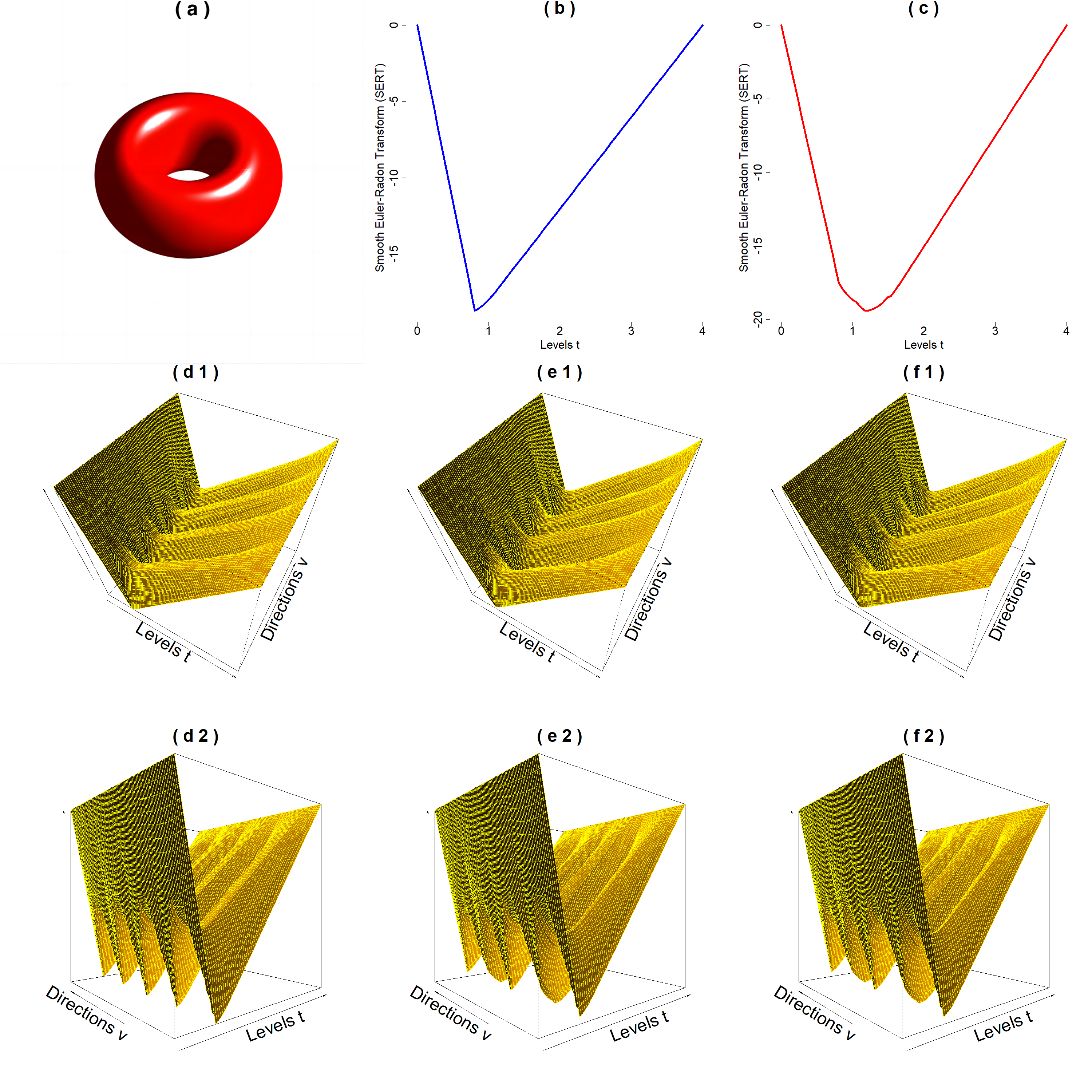
Figure 3: The torus in panel (a) presents the level set $\{x\in\mathbb{R}^{3}:\,g(x)=0.0834\}$, where $g$ is defined in Eq. (5.1). Panel (b) presents curve $t\mapsto\operatorname{SERT}(g)(\nu,t)$ with $\nu=(0,1,0)^{\intercal}$. Panel (c) presents curve $t\mapsto\operatorname{SERT}(g)(\nu,t)$ with $\nu=(0,0,1)^{\intercal}$. Panels (d1, d2, e1, e2, f1, f2) present the surfaces $(\theta,t)\mapsto\operatorname{SERT}(g)(\nu,t)$ with different directions $\nu$ as in Eq. (5.2). Panels (d1, d2) present the same surface from different angles. Similar for panels (e1, e2) and (f1, f2).

5 A Proof-of-Concept Example

Our proposed SERT plays an important role in the statistical inference discussed in Section 5, given its ability to convert grayscale images into functional data. Before delving into the SERT-based statistical inference, in this section, we illustrate the SERT via a proof-of-concept example. Here, we focus on dimensionality $d=3$ and the following scalar field

$$g(x):=\left\{\left(\sqrt{\frac{3}{4}\left(x_{1}^{2}+x_{2}^{2}\right)}-\frac{1}{2}\right)^{2}+\frac{3x_{3}^{2}}{4}\right\}\cdot\mathbbm{1}_{\{-1\leq x_{1},\,x_{2},\,x_{3}\leq 1\}},\ \ \ \text{ where }x=(x_{1},x_{2},x_{3})^{\intercal}.$$ (5.1)

The $g$ in Eq. (5.1) is a grayscale function (in the sense of Definition 3.3), where $g\in\mathfrak{D}_{R,d}$ with $d=3$ and $R=2$. A level set $\{x\in\mathbb{R}^{3}:\,g(x)=0.0834\}$ of $g$ is presented in Figure 3 (the level 0.0834 was specifically chosen to make the visualization of the level set look like a torus). We computed the ERT of the $g$ in a sequential manner. We first compute the LECT and SELECT using the MATLAB isosurface procedure. Next, we compute the ERT utilizing the Lebesgue integration representation in Eq. (4.6). Finally, the SERT is derived from the ERT via a standard numerical integration method.

The SERT of the $3$-dimensional grayscale image $g$ defined in Eq. (5.1) is a scalar field over the 3-dimensional product manifold $\mathbb{S}^{2}\times[0,4]$, where $(\nu,t)\mapsto\operatorname{SERT}(g)(\nu,t)$ with $\nu=(\nu_{1},\nu_{2},\nu_{3})^{\intercal}\in\mathbb{S}^{2}$. We visualize the following segments of the scalar field

$$\begin{aligned} &(\theta,t)\mapsto\operatorname{SERT}(g)(\nu,t)\ \text{with}\ \nu=(\cos\theta,\,\sin\theta,\,0)^{\intercal}\ \text{in Figure \ref{fig: Merged_document}(d1, d2)};\\ &(\theta,t)\mapsto\operatorname{SERT}(g)(\nu,t)\ \text{with}\ \nu=(\cos\theta,\,0,\,\sin\theta)^{\intercal}\ \text{in see Figure \ref{fig: Merged_document}(e1, e2)};\\ &(\theta,t)\mapsto\operatorname{SERT}(g)(\nu,t)\ \text{with}\ \nu=(0,\,\cos\theta,\,\sin\theta)^{\intercal}\ \text{in Figure \ref{fig: Merged_document}(f1, f2)};\end{aligned}$$ (5.2)

where $\theta\in[0,2\pi]$ and $t\in[0,4]$. The maps in Eq. (5.2) are scalar fields over $[0,2\pi]\times[0,4]$ and are presented in the second and third rows of Figure 3.

In Figure 3, the surfaces corresponding to $(\theta,t)\mapsto\operatorname{SERT}(g)(\nu,t)$ consistently exhibit an approximate periodicity of $\pi/2$ in the variable $\theta$ (indicated by the axis label “Direction $\nu$”). This approximate periodicity is fundamentally derived from the “box-shape” indicator function $\mathbbm{1}_{\{-1\leq x_{1},,x_{2},,x_{3}\leq 1\}}$ in Eq. (5.1). The surfaces depicted in Figures 3(e1, e2) and 3(f1, f2) are indistinguishable, which is a characteristic attributed to the $x_{1}$-$x_{2}$ symmetry of the grayscale function $g$ defined in Eq. (5.1). The surfaces presented in Figure 3(d1, d2) exhibit subtle distinctions from those in 3(e1, e2, f1, f2). The curves and surfaces in Figure 3, as well as the scalar field $(\nu,t)\mapsto\operatorname{SERT}(g)(\nu,t)$, suggest a potential association of the SERT with manifold learning (Yue et al., 2016, Dunson and Wu, 2021, Meng and Eloyan, 2021, Li et al., 2022).

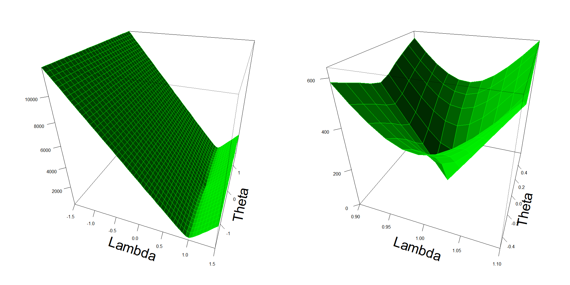
Figure 4: The left panel presents the surface of the function defined in Eq. (6.7) for $\theta\in[-\pi/2,\,\pi/2]$ and $\lambda\in[-3/2,\,3/2]$. Notably, we have also considered the negative scaling parameters $\lambda<0$, which correspond to the “white-to-black” transition. The right panel presents the same function with $\theta\in[-0.45,\,0.45]$ and $\lambda\in[0.9,\,1.1]$. Both surfaces indicate that the function in Eq. (6.7) is minimized when $\lambda=1$ and $\theta=0$.

6 Alignment of Images and Invariance of the ERT

In various applications, images are typically aligned before analysis (e.g., Bankman, 2008). Wang et al. (2021) utilized an ECT-based approach to align shapes (equivalently, binary images) through orthogonal actions. The primary aim of the ECT-based strategy is to lessen the difference between a pair of shapes resulting from the orthogonal movements. An in-depth exposition of the ECT-based method, along with a proof-of-concept example, can be found in Supplementary Section 4 of Wang et al. (2021). Analogous correspondence free alignment techniques are also needed for grayscale images. Kirveslahti and Mukherjee (2023) examined the invariance of the LECT with respect to orthogonal alignments and introduced an LECT/SELECT-based alignment method tailored for grayscale images. Motivated by the studies in both Wang et al. (2021) and Kirveslahti and Mukherjee (2023), in this section, we introduce an ERT-based alignment approach. This approach will serve as a preprocessing step for the ERT-based statistical inference detailed in Section 7.

Let $g^{\diamondsuit}$ represent a reference image designated as a template. For any source image $g$ under consideration, we consider a collection of transforms, denoted by $\mathscr{T}$, encompassing all transformations $T$ of interest. From $\mathscr{T}$, we select the transformation $T^{\blacklozenge}\in\mathscr{T}$ such that the transformed image $T^{\blacklozenge}(g)$ is the most similar to $g^{\diamondsuit}$ based on a specified dissimilarity metric. Subsequent analysis is then conducted on the aligned image $T^{\blacklozenge}(g)$ instead of the original source image $g$. A potential choice for the dissimilarity metric can be one of the distances defined in Eq.(4.7), denoted as $\operatorname{dist}$. This can be summarized as follows

$$T^{\blacklozenge}:=\operatorname*{arg\,min}_{T\in\mathscr{T}}\,\operatorname{dist}\Big{(}g^{\diamondsuit},T(g)\Big{)}.$$ (6.1)

Beyond the orthogonal actions implemented in Wang et al. (2021) and Kirveslahti and Mukherjee (2023), we also consider scaling transforms of grayscale images, including the “white-to-black” transition. In this paper, we focus on the following collection of transforms

$$\mathscr{T}=\left\{T:\,(Tg)(x)=\lambda\cdot g(\boldsymbol{A}^{-1}x),\text{ where }\lambda\in\mathbb{R}\text{ and }\boldsymbol{A}\in\operatorname{O}(d)\right\},$$ (6.2)

where $\operatorname{O}(d)$ denotes the orthogonal group in dimension $d$, and it contains all the rotations and reflections in $\mathbb{R}^{d}$. For ease of notation, we define the dual $\boldsymbol{A}_{*}$ of $\boldsymbol{A}$ by $(\boldsymbol{A}_{*}g)(x):=g\left(\boldsymbol{A}^{-1}x\right)$. The goal of employing minimization across the collection in Eq. (6.2) is to mitigate disparities between two images arising from orthogonal movements and variations in pixel intensity scales.

A challenge in using the criterion presented in Eq. (6.1), combined with any of the dissimilarity metrics in Eq.(4.7), is the computational cost of obtaining $\operatorname{ERT}(T(g))$ for all $T\in\mathscr{T}$. More specifically, the computation of $\operatorname{ERT}(\lambda\cdot\boldsymbol{A}_{*}g)$ is required for every $\lambda\in\mathbb{R}$ and $\boldsymbol{A}\in\operatorname{O}(d)$. Fortunately, the homogeneity of the ERT (see Theorem 3.2) implies $\operatorname{ERT}(\lambda\cdot\boldsymbol{A}_{*}g)=\lambda\cdot\operatorname{ERT}(\boldsymbol{A}_{*}g)$ for all $\lambda\in\mathbb{R}$. Therefore, we can simply calculate $\operatorname{ERT}(\boldsymbol{A}_{*}g)$ and get the $\operatorname{ERT}(\lambda\cdot\boldsymbol{A}_{*}g)$ for all $\lambda\in\mathbb{R}$ by simply scaling the computed $\operatorname{ERT}(\boldsymbol{A}_{*}g)$. Similarly, if we further have the “$\boldsymbol{A}_{*}$-homogeneity”, where “$\operatorname{ERT}(\boldsymbol{A}_{*}g)=\boldsymbol{A}_{*}\operatorname{ERT}(g)$,” the amount of computation required in Eq. (6.1) is further reduced. The “$\boldsymbol{A}_{*}$-homogeneity” is true and accurately presented by the following result.

Theorem 6.1.

For any $g\in\mathfrak{D}_{R,d}$ and $\boldsymbol{A}\in\operatorname{O}(d)$, we have $\operatorname{ECT}(\boldsymbol{A}_{*}g)(\nu,t)=\operatorname{ECT}(g)(\boldsymbol{A}^{-1}\nu,t)=:\boldsymbol{A}_{*}\operatorname{ECT}(g)(\nu,t)$ for all $\nu\in\mathbb{S}^{d-1}$ and $t\in[0,T]$.

Theorem 6.1 is a direct result of “Proposition 2.18” of Kirveslahti and Mukherjee (2023) via Eq. (4.6); hence, we omit its proof. Combining the scalar homogeneity and $\boldsymbol{A}_{*}$-homogeneity, we have the following

$$\operatorname{ECT}(\lambda\cdot\boldsymbol{A}_{*}g)(\nu,t)=\lambda\cdot\operatorname{ECT}(g)(\boldsymbol{A}^{-1}\nu,t)=:\lambda\cdot\boldsymbol{A}_{*}\operatorname{ECT}(g)(\nu,t),$$ (6.3)

for all $g\in\mathfrak{D}_{R,d}$, $\nu\in\mathbb{S}^{d-1}$, and $t\in[0,T]$. Using $\operatorname{dist}=\operatorname{dist}^{\operatorname{ERT}}_{p,q}$ as an example (see Eq. (4.7) for the definition of $\operatorname{dist}^{\operatorname{ERT}}_{p,q}$), an optimal transformation across the collection in Eq. (6.2) can be represented via Eq. (6.3) as follows

$$\operatorname*{arg\,min}_{\lambda\in\mathbb{R}\text{ and }\boldsymbol{A}\in\operatorname{O}(d)}\,\left\|\,\operatorname{ERT}(g)-\lambda\cdot\boldsymbol{A}_{*}\operatorname{ERT}(g)\,\right\|_{L_{\nu}^{q}L_{t}^{p}}.$$ (6.4)

In Eq. (6.4), we only need to compute the ERT of $g^{\diamondsuit}$ and $g$ instead of all the $\lambda\cdot\boldsymbol{A}_{*}g$ for all $\lambda\in\mathbb{R}$ and $\boldsymbol{A}\in\operatorname{O}(d)$. Notably, when both $g^{\diamondsuit}$ and $g$ are indicator functions representing constructible sets, the alignment method detailed in Eq. (6.4) is equivalent to the ECT-based alignment method proposed in Wang et al. (2021).

To illustrate the performance of the alignment approach described in Eq. (6.4), we present a proof-of-concept example. Our benchmark criterion for assessing the efficacy of the alignment approach is its ability to eliminate differences between images arising from rotation and scaling. Let $g$ denote the grayscale function defined in Eq. (5.1). We will study the scaled and rotated version $\lambda\cdot\boldsymbol{A}_{\theta,*}g$ of $g$, where $\boldsymbol{A}_{\theta,*}$ denotes the dual of the rotation matrix $\boldsymbol{A}_{\theta}$ defined as

$$\boldsymbol{A}_{\theta}:=\begin{pmatrix}\cos\theta&0&\sin\theta\\ 0&1&0\\ -\sin\theta&0&\cos\theta\end{pmatrix},$$ (6.5)

which represents rotation on the $(x_{1},x_{3})$-plane by angle $\theta$. Obviously, the differences between the source image $\lambda\cdot\boldsymbol{A}_{\theta,*}g$ and the reference image $g$ vanish if and only if $\theta=0$ and $\lambda=1$ (i.e., no rotation or scaling). Hence, in this example, our proposed alignment approach is effective if

$$(0,1)=\operatorname*{arg\,min}_{(\theta,\lambda)}\left\{\left\|\,\operatorname{ERT}(g)-\lambda\cdot\boldsymbol{A}_{\theta,*}\operatorname{ERT}(g)\,\right\|_{L_{\nu}^{2}L_{t}^{2}}\right\}.$$ (6.6)

To validate Eq. (6.6), we analyze the surface of the following function of $(\theta,\lambda)$

$$(\theta,\lambda)\mapsto\left\|\,\operatorname{ERT}(g)-\lambda\cdot\boldsymbol{A}_{\theta,*}\operatorname{ERT}(g)\,\right\|_{L_{\nu}^{2}L_{t}^{2}},$$ (6.7)

which is presented in Figure 4. The surfaces presented in Figure 4 confirm the minimization in Eq. (6.6) — the minimum point of the surface corresponds to the coordinates $(\theta,\lambda)=(0,1)$, implying that our alignment approach delineated in Eq. (6.4) is effective.

To illustrate the performance of the proposed alignment approach in our proof-of-concept example, we consider the $g$ defined in Eq. (5.1) as the reference image, as depicted in Figure 5(a). Next, $\lambda\cdot\mathbf{A}_{\theta,*}g(x)$ with parameters $(\theta,\lambda)=(\pi/6,\,1/5)$ is selected as the source image, as illustrated in Figure 5(b). The source image is a rotated and scaled version of the reference image. Aligning the source image with respect to the reference yields the post-aligned source image shown in Figure 5(c). The reference image in Figure 5(a) and post-aligned source image in Figure 5(c) are nearly congruent. This similarity underscores the efficacy of the proposed alignment methodology in mitigating discrepancies attributable to rotations and scaling.

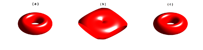
Figure 5: In panel (a), the level set $\{x\in\mathbb{R}^{3}:g(x)=0.0834\}$ is illustrated with $g$ being defined as in Eq. (5.1). Panel (b) depicts the level set $\{x\in\mathbb{R}^{3}:\lambda\cdot\mathbf{A}_{\theta,*}g(x)=0.0834\}$ for parameters $\lambda=1/5$ and $\theta=\pi/6$. Here, we consider $g$ to be the reference image and $\lambda\cdot\mathbf{A}_{\theta,*}g(x)$ with $(\theta,\lambda)=(\pi/6,\,1/5)$ representing the source image that is under investigation. Panels (a) and (b) show that the reference and source images are drastically different. Employing the methodology from Eq. (6.4), we align $\lambda\cdot\mathbf{A}_{\theta,*}g(x)$ which results in the aligned image denoted as $\tilde{g}$. Panel (c) showcases the level set $\{x\in\mathbb{R}^{3}:\tilde{g}(x)=0.0834\}$, closely mirroring the level set displayed in panel (a).

7 Statistical Inference of Grayscale Functions

We now provide our second major contribution — approaches for statistical inference on grayscale images. The grayscale functions presented in the previous sections of this work have been viewed as deterministic. In this section, we now view grayscale functions as random where we assume that they are generated from underlying distributions satisfying some regularity conditions (see Assumptions 2 and 3 in Section 7.1). Let $\Omega$ denote the collection of grayscale functions of interest, and assume that $\Omega$ is equipped with a $\sigma$-field $\mathscr{F}$. Next, suppose that there are two underlying grayscale function-generating distributions (probability measures), $\mathbb{P}^{(1)}$ and $\mathbb{P}^{(2)}$, defined on the sample space $(\Omega,\mathscr{F})$. Our data are two collections of random grayscale functions sampled from the two distributions: $\{g_{i}^{(1)}\}_{i=1}^{n}\overset{iid}{\sim}\mathbb{P}^{(1)}$ and $\{g_{i}^{(2)}\}_{i=1}^{n}\overset{iid}{\sim}\mathbb{P}^{(2)}$. Here, we provide approaches to testing if the two collections of functions are significantly different. More precisely, we propose methods of testing the following hypotheses

$$H_{0}^{*}:\ \ \mathbb{P}^{(1)}=\mathbb{P}^{(2)}\ \ \ \text{vs.}\ \ \ H_{1}^{*}:\ \ \mathbb{P}^{(1)}\neq\mathbb{P}^{(2)}.$$ (7.1)

Without loss of generality, hereafter, we assume that the grayscale images $\{g_{i}^{(1)}\}_{i=1}^{n}$ and $\{g_{i}^{(2)}\}_{i=1}^{n}$ have been aligned using the ERT-based alignment method proposed in Section 6.

7.1 $\chi^{2}$-test via the Karhunen–Loève Expansion

In this subsection, we propose $\chi^{2}$-based hypothesis testing procedures via the Karhunen–Loève expansion and central limit theorem (CLT). These can be as generalizations of results presented in Meng et al. (2022) for the SECT and binary images. Testing the hypotheses in Eq. (7.1) is a highly nonparametric problem, and the $\chi^{2}$-test approaches transform it into a parametric problem.

Suppose the grayscale image $g$ is random and $g\sim\mathbb{P}^{(j)}$ for either $j=1$ or $j=2$. For each fixed $(\nu,t)\in\mathbb{S}^{d-1}\times[0,T]$, we have $\operatorname{SERT}(g)(\nu,t)$ as a real-valued random variable. Hence, for each fixed direction $\nu\in\mathbb{S}^{d-1}$, $\operatorname{SECT}(g)(\nu):=\{\operatorname{SERT}(g)(\nu,t)\}_{t\in[0,T]}$ is a stochastic process. Note that it is straightforward that the sample paths of the stochastic process are continuous (see Eq. (3.12)). In this section, we assume the following regarding $\mathbb{P}^{(1)}$ and $\mathbb{P}^{(2)}$.

Assumption 2.

For each $j\in\{1,2\}$ and $(\nu,t)\in\mathbb{S}^{d-1}\times[0,T]$, we have the finite second moment $\mathbb{E}^{(j)}\left|\operatorname{SERT}(\nu,t)\right|^{2}:=\int_{\Omega}|\operatorname{SERT}(g)(\nu,t)|^{2}\,\mathbb{P}^{(j)}(dg)<\infty$.

Under Assumption 2, we define the mean and covariance functions of $\operatorname{SECT}(g)(\nu)$ as follows

$$m_{\nu}^{(j)}(t):=\mathbb{E}^{(j)}\left\{\operatorname{SERT}(\nu,t)\right\}=\int_{\Omega}\operatorname{SERT}(g)(\nu,t)\,\mathbb{P}^{(j)}(dg),$$

$$\kappa_{\nu}^{(j)}(s,t):=\int_{\Omega}\Big{(}\operatorname{SERT}(g)(\nu,s)-m_{\nu}^{(j)}(s)\Big{)}\cdot\Big{(}\operatorname{SERT}(g)(\nu,t)-m_{\nu}^{(j)}(t)\Big{)}\,\mathbb{P}^{(j)}(dg),$$

for $j\in\{1,2\}$, $\nu\in\mathbb{S}^{d-1}$, and $s,t\in[0,T]$, where $\mathbb{E}^{(j)}$ denotes the expectation associated with the probability measure $\mathbb{P}^{(j)}$. Furthermore, we need the following assumption on the covariance functions.

Assumption 3.

For each $j\in\{1,2\}$ and fixed $\nu\in\mathbb{S}^{d-1}$, the function $(s,t)\mapsto\kappa_{\nu}^{(j)}(s,t)$ is continuous on the product space $[0,T]\times[0,T]$.

Under Assumption 3, the stochastic process $\operatorname{SECT}(g)(\nu)$ is mean-square continuous, which is a direct result of “Lemma 4.2” of Alexanderian (2015). The mean-square continuity implies that $t\mapsto m_{\nu}^{(j)}(t)$ is a continuous function over the compact interval $[0,T]$.

Distinguishing the two collections of grayscale images, $\{g_{i}^{(1)}\}_{i=1}^{n}\overset{iid}{\sim}\mathbb{P}^{(1)}$ and $\{g_{i}^{(2)}\}_{i=1}^{n}\overset{iid}{\sim}\mathbb{P}^{(2)}$, is done by rejecting the null hypothesis $H_{0}^{*}$ in Eq. (7.1). To reject the null $H_{0}^{*}$ in Eq. (7.1), it suffices to reject the null hypothesis $H_{0}$ in the following test

$$\begin{aligned} &H_{0}:\,m_{\nu^{*}}^{(1)}(t)=m_{\nu^{*}}^{(2)}(t)\text{ for all }t\in[0,T]\ \ \ vs.\ \ \ H_{1}:\,m_{\nu^{*}}^{(1)}(t^{\prime})=m_{\nu^{*}}^{(2)}(t^{\prime})\text{ for some }t^{\prime}\in[0,T],\\ &\text{where }\ \ \nu^{*}:=\operatorname*{\arg\!\max}_{\nu\in\mathbb{S}^{d-1}}\left\{\sup_{t\in[0,T]}\left|m_{\nu^{*}}^{(1)}(t)-m_{\nu^{*}}^{(2)}(t)\right|\right\}.\end{aligned}$$ (7.2)

We need the following assumption to perform a $\chi^{2}$-test for the hypotheses in Eq. (7.2).

Assumption 4.

$\kappa_{\nu^{*}}^{(1)}=\kappa_{\nu^{*}}^{(2)}$ where the direction $\nu^{*}$ is defined in Eq. (7.2).

Assumption 4 is true under the null $H_{0}^{*}:\mathbb{P}^{(1)}=\mathbb{P}^{(2)}$ in Eq. (7.1). Under Assumption 4, we denote $\kappa:=\kappa_{\nu^{*}}^{(1)}=\kappa_{\nu^{*}}^{(2)}$. Under Assumption 3, we have $\kappa\in L^{2}([0,T]\times[0,T])$ which further implies that the integral operator $f\mapsto\int_{0}^{T}f(s)\cdot\kappa(s,\cdot)\,ds$ defined on $L^{2}(0,T)$ is a compact, positive, and self-adjoint (see “Lemma 5.1” of Alexanderian (2015)). The Hilbert-Schmidt theorem (see “Theorem VI.16” of Reed (2012)) indicates that this integral operator has countably many orthonormal eigenfunctions $\{\phi_{l}\}_{l=1}^{\infty}$ and nonnegative eigenvalues $\{\lambda_{l}\}_{l=1}^{\infty}$. Without loss of generality, we assume $\lambda_{1}\geq\lambda_{2}\geq\ldots\geq 0$. Following the proof of the “Karhunen-Loève expansion” in Meng et al. (2022), one can show the following result.

Theorem 7.1.

Suppose $g^{(1)}\sim\mathbb{P}^{(1)}$ and $g^{(2)}\sim\mathbb{P}^{(2)}$ are independent. Let $\mathbb{P}^{(1)}\otimes\mathbb{P}^{(2)}$ denote a product probability measure. For each fixed $l\in\mathbb{N}$, the following identity holds with probability one

$$\frac{1}{\sqrt{2\lambda_{l}}}\int_{0}^{T}\left\{\,\operatorname{SERT}(g^{(1)})(\nu^{*},t)-\operatorname{SERT}(g^{(2)})(\nu^{*},t)\,\right\}\cdot\phi_{l}(t)\,dt=\theta_{l}+\left(\frac{Z_{l}^{(1)}(g^{(1)})-Z_{l}^{(2)}(g^{(1)})}{\sqrt{2}}\right),$$ (7.3)

that is, $\mathbb{P}^{(1)}\otimes\mathbb{P}^{(2)}\left\{\text{Eq.\leavevmode\nobreak\ \eqref{eq: Karhunen–Loève expansion} holds}\right\}=1$, where,

$$\begin{aligned} &\theta_{l}:=\frac{1}{\sqrt{2\lambda_{l}}}\int_{0}^{T}\left\{\,m_{\nu^{*}}^{(1)}(t)-m_{\nu^{*}}^{(2)}(t)\,\right\}\cdot\phi_{l}(t)\,dt,\\ &Z_{l}^{(j)}(g)=\frac{1}{\sqrt{\lambda_{l}}}\int_{0}^{T}\left\{\,\operatorname{SECT}(g)(\nu^{*},t)-m_{\nu^{*}}^{(j)}(t)\,\right\}\cdot\phi_{l}(t)\,dt,\ \ \ \text{ for }j\in\{1,2\}.\end{aligned}$$ (7.4)

Furthermore, for each $j\in\{1,2\}$, random variables $\{Z_{l}^{(j)}\}_{l=1}^{\infty}$ are defined on the probability space $(\Omega,\mathscr{F},\mathbb{P}^{(j)})$, mutually uncorrelated, and have mean 0 and variance 1.

Following the discussion in Meng et al. (2022), one can show that the null hypothesis $H_{0}$ in Eq. (7.2) is equivalent to $\theta_{l}=0$ for all $l=1,2,3,\ldots$. It is infeasible to check $\theta_{l}$ for all positive integers $l$. In addition, a small $\lambda_{l}$ in the denominator (e.g., see Eq. (7.4)) induces numerical instability. Therefore, we only consider $\theta_{l}$ for $l=1,2,\ldots,L$, where $L$ is given as the following

$$L:=\min\left\{\,k\in\mathbb{N}\,:\,\frac{\sum_{k^{\prime}=1}^{k}\lambda_{k^{\prime}}}{\sum_{k^{\prime\prime}=1}^{\infty}\lambda_{k^{\prime\prime}}}>0.99\right\}.$$ (7.5)

Here, 0.99 can be replaced with any value in $(0,\,1)$; we take 0.99 as an example. The $L$ defined in Eq. (7.5) is motivated by principal component analysis (Jolliffe, 2002) and indicates that we maintain at least $99\%$ of the cumulative variance in the data. Hence, to test the hypotheses in Eq. (7.2), we may test the following approximate hypotheses

$$\widehat{H_{0}}:\,\theta_{0}=\theta_{1}=\cdots=\theta_{L}=0\ \ \ vs.\ \ \ \widehat{H_{1}}:\,\text{there exists }k^{\prime}\in\{1,2,\ldots,L\}\text{ such that }\theta_{k^{\prime}}\neq 0.$$ (7.6)

Given data $\{g^{(1)}_{i}\}_{i=1}^{n}\overset{iid}{\sim}\mathbb{P}^{(1)}$ and $\{g^{(2)}_{i}\}_{i=1}^{n}\overset{iid}{\sim}\mathbb{P}^{(2)}$, the approximate hypotheses in Eq. (7.6) can be tested using the random variables $\{\xi_{l,i}:\,l=1,\ldots,L\text{ and }i=1,\ldots,n\}$ defined as follows

$$\xi_{l,i} :=\frac{1}{\sqrt{2\lambda_{l}}}\int_{0}^{T}\left\{\,\operatorname{SERT}(g_{i}^{(1)})(\nu^{*},t)-\operatorname{SERT}(g_{i}^{(2)})(\nu^{*},t)\,\right\}\cdot\phi_{l}(t)\,dt=\theta_{l}+\left(\frac{Z_{l}^{(1)}(g_{i}^{(1)})-Z_{l}^{(2)}(g_{i}^{(1)})}{\sqrt{2}}\right).$$

Theorem 7.5 implies that the random variables $\xi_{l,i}$ satisfy the following properties:

• For each $l\in\{1,\ldots,L\}$ and $i\in\{1,\ldots,n\}$, the random variable $\xi_{l,i}$ has mean $\theta_{l}$ and variance 1.

• For each fixed $i\in\{1,\ldots,n\}$, the random variables $\xi_{1,i},\ldots,\xi_{L,i}$ are mutually uncorrelated.

• For each fixed $l\in\{1,\ldots,L\}$, the random variables $\xi_{l,1},\ldots,\xi_{l,n}$ are iid.

The properties above indicate:

1. For each fixed $l\in\{1,\ldots,L\}$, the standardized $\frac{1}{\sqrt{n}}\sum_{i=1}^{n}\xi_{l,i}$ asymptotically follows a standard Gaussian distribution $N(0,1)$ under the null hypothesis $\widehat{H_{0}}$ in Eq. (7.6).

2. The asymptotic normality implies that random variables $\frac{1}{\sqrt{n}}\sum_{i=1}^{n}\xi_{1,i},\ldots,\frac{1}{\sqrt{n}}\sum_{i=1}^{n}\xi_{L,i}$ are asymptotically independent.

Hence, $\sum_{l=1}^{L}\left(\frac{1}{\sqrt{n}}\sum_{i=1}^{n}\xi_{l,i}\right)^{2}$ is asymptotically $\chi^{2}_{L}$ under the null hypothesis $\widehat{H_{0}}$ in Eq. (7.6), and we reject $\widehat{H_{0}}$ with asymptotic significance $\alpha\in(0,1)$ if

$$\sum_{l=1}^{L}\left(\frac{1}{\sqrt{n}}\sum_{i=1}^{n}\xi_{l,i}\right)^{2}>\chi_{L,1-\alpha}^{2}=\text{ the $1-\alpha$ lower quantile of the $\chi^{2}_{L}$ distribution}.$$ (7.7)

Overall, we summarize our hypothesis testing problem as follows. Our goal is to test the hypotheses in Eq. (7.1). Through the Karhunen–Loève expansion (see Theorem 7.1), it suffices to test the approximate hypotheses in Eq. (7.6), which can be achieved by the $\chi^{2}$-test in Eq. (7.7).

Suppose we have two groups of grayscale functions, $\{g^{(1)}_{i}\}_{i=1}^{n}\overset{iid}{\sim}\mathbb{P}^{(1)}$ and $\{g^{(2)}_{i}\}_{i=1}^{n}\overset{iid}{\sim}\mathbb{P}^{(2)}$. We calculate the discretized SERT of the grayscale images, denoted as $\mathcal{D}^{(j)}:=\{\operatorname{SERT}(g_{i}^{(j)})(\nu_{p},t_{q}):\,p=1,\ldots,\Gamma\text{ and }q=1,\ldots,\Delta\}_{i=1}^{n}$ for $j\in\{1,2\}$. Then, we apply $\mathcal{D}^{(1)}$ and $\mathcal{D}^{(2)}$ as our input data to test the hypotheses in Eq. (7.2), which are approximated by that in Eq. (7.6). We may apply “Algorithm 1” in Meng et al. (2022) to test the hypotheses in Eq. (7.6) by simply replacing the “SECT of two collections of shapes” therein with the “SERT of two collections of grayscale functions”. The replacing of the SECT with SERT approach is explicitly summarized in Algorithm 1.

Algorithm 1 : $\chi^{2}$-test

1:(i) Two collections $\{g_{i}^{(1)}\}_{i=1}^{n}$ and $\{g_{i}^{(2)}\}_{i=1}^{n}$ of grayscale functions; (ii) desired asymptotic confidence level $1-\alpha$ with asymptotic significance $\alpha\in(0,1)$.

2:Accept or Reject the null hypothesis $\widehat{H_{0}}$ in Eq. (7.6). (Rejecting the $\widehat{H_{0}}$ implies rejecting the null hypothesis $H_{0}^{*}$ in Eq. (7.1).)

3:Compute the discretized SERT $\{\operatorname{SERT}(g_{i}^{(j)})(\nu_{p},t_{q}):\,p=1,\ldots,\Gamma\text{ and }q=1,\ldots,\Delta\}_{i=1}^{n}$ for $j\in\{1,2\}$ of the input grayscale functions.

4:Replace the input “SECT” in “Algorithm 1” of Meng et al. (2022) with the SERT computed in the previous step.

5:Implement “Algorithm 1” of Meng et al. (2022) and get the output.

Although the null hypothesis in Eq. (7.1) theoretically implies Assumption 4, the finite sample size $n<\infty$ may numerically violate Assumption 4 due to the inaccuracy in the estimation of covariance functions. The (numerical) violation of Assumption 4 tends to lead to type-I error inflation. To reduce the type-I error rate, we apply a permutation technique (Good, 2013). That is, we first apply Algorithm 1 to our original grayscale images $g_{i}^{(j)}$ and then repeatedly re-apply Algorithm 1 to the grayscale images with shuffled group labels $j$. Next, we compare how the $\chi^{2}$ statistic derived from the original data (see Eq. (7.7)) differs from that computed on the shuffled data. The idea behind the permutation approach is that shuffling the group labels $j$ of images $g_{i}^{(j)}$ should not significantly change the test statistic under the null hypothesis. The combination of the permutation technique and Algorithm 1 is an analog of the permutation test proposed in Meng et al. (2022). We summarize this method in Algorithm 2. Among the algorithms we propose throughout, we particularly recommend using Algorithm 2 in practice — this is also supported by simulation study results presented in Section 8. Specifically, we will show that Algorithm 2 is uniformly powerful under the alternative hypotheses and does not suffer from type I error inflation.

Algorithm 2 : Permutation-based $\chi^{2}$-test

1:(i) Two collections $\{g_{i}^{(1)}\}_{i=1}^{n}$ and $\{g_{i}^{(2)}\}_{i=1}^{n}$ of grayscale functions; (ii) desired asymptotic confidence level $1-\alpha$ with asymptotic significance $\alpha\in(0,1)$; (iii) the number of permutations $\Pi$.

2:Accept or Reject the null hypothesis $\widehat{H_{0}}$ in Eq. (7.6). (Rejecting the $\widehat{H_{0}}$ implies rejecting the null hypothesis $H_{0}^{*}$ in Eq. (7.1).)

3:Compute the discretized SERT $\{\operatorname{SERT}(g_{i}^{(j)})(\nu_{p},t_{q}):\,p=1,\ldots,\gamma\text{ and }q=1,\ldots,\Delta\}_{i=1}^{n}$ for $j\in\{1,2\}$ of the input grayscale functions.

4:Replace the input “SECT” in “Algorithm 2” of Meng et al. (2022) with the SERT computed in the previous step.

5:Implement “Algorithm 2” of Meng et al. (2022) and get the output.

7.2 Full Permutation Test

In Section 7.1, we proposed two parametric-based approaches — Algorithms 1 and 2 — to testing the hypotheses in Eq. (7.1). Although Algorithm 2 involves a permutation-like technique, it still heavily depends on the $\chi^{2}$-test in Eq. (7.7). In contrast, we also propose a full permutation hypothesis test. We will also compare this approach with Algorithms 1 and 2 using simulations in Section 8. The simulation studies therein indicate that our proposed Algorithms 1 and 2 tend to be more powerful than the fully permutation-based test. Following a strategy proposed by Robinson and Turner (2017), we apply the full permutation test based on the following loss function

$$L\left(\{g_{i}^{(1)}\}_{i=1}^{n},\,\{g_{i}^{(2)}\}_{i=1}^{n}\right):=\frac{1}{2n(n-1)}\sum_{k,l=1}^{n}\left\{\,\operatorname{dist}\left(\,g_{k}^{(1)},\,g_{l}^{(1)}\,\right)+\operatorname{dist}\left(\,g_{k}^{(2)},\,g_{l}^{(2)}\,\right)\,\right\},$$ (7.8)

where $\operatorname{dist}\in\{\operatorname{dist}^{\operatorname{ERT}}_{p,q},\operatorname{dist}^{\operatorname{SERT}}_{p,q},\operatorname{dist}^{\operatorname{SELECT}}_{p},\operatorname{dist}^{\operatorname{MEC}}_{p}\}$ (see Eq. (4.7) and Eq. (4.8)). The full permutation test based on Eq. (7.8) is summarized in Algorithm 3.

Algorithm 3 : Full Permutation Test

1:(i) Two collections $\{g_{i}^{(1)}\}_{i=1}^{n}$ and $\{g_{i}^{(2)}\}_{i=1}^{n}$ of grayscale functions; (ii) desired asymptotic confidence level $1-\alpha$ with $\alpha\in(0,1)$; (iii) the number $\Pi$ of permutations; (iv) distance function $\operatorname{dist}\in\{\operatorname{dist}^{\operatorname{ERT}}_{p,q},\operatorname{dist}^{\operatorname{SERT}}_{p,q},\operatorname{dist}^{\operatorname{SELECT}}_{p},\operatorname{dist}^{\operatorname{MEC}}_{p}\}$ with prespecified parameters $p$ and $q$.

2:Accept or Reject the null hypothesis $H_{0}^{*}$ in Eq. (7.1).

3:Apply Eq. (7.8) to the original input grayscale functions and compute the value of the loss

$$\mathfrak{S}_{0}:=L\left(\{g_{i}^{(1)}\}_{i=1}^{n},\,\{g_{i}^{(2)}\}_{i=1}^{n}\right).$$

4:for all $k=1,\cdots,\Pi$,  do

5:   Randomly permute the group labels $j\in\{1,2\}$ of the input grayscale functions where the permuted grayscale functions are denoted as $\{\tilde{g}_{i}^{(1)}\}_{i=1}^{n}$ and $\{\tilde{g}_{i}^{(2)}\}_{i=1}^{n}$.

6:   Apply Eq. (7.8) to the permuted grayscale functions and compute the value of the loss

$$\mathfrak{S}_{k}:=L\left(\{\tilde{g}_{i}^{(1)}\}_{i=1}^{n},\,\{\tilde{g}_{i}^{(2)}\}_{i=1}^{n}\right).$$

7:end for

8:Compute $k^{*}:=\lfloor\alpha\cdot\Pi\rfloor:=$ the largest integer smaller than $\alpha\cdot\Pi$.

9:Reject the null hypothesis $H_{0}$ if $\mathfrak{S}_{0}<\mathfrak{S}_{k^{*}}$ and report the output.

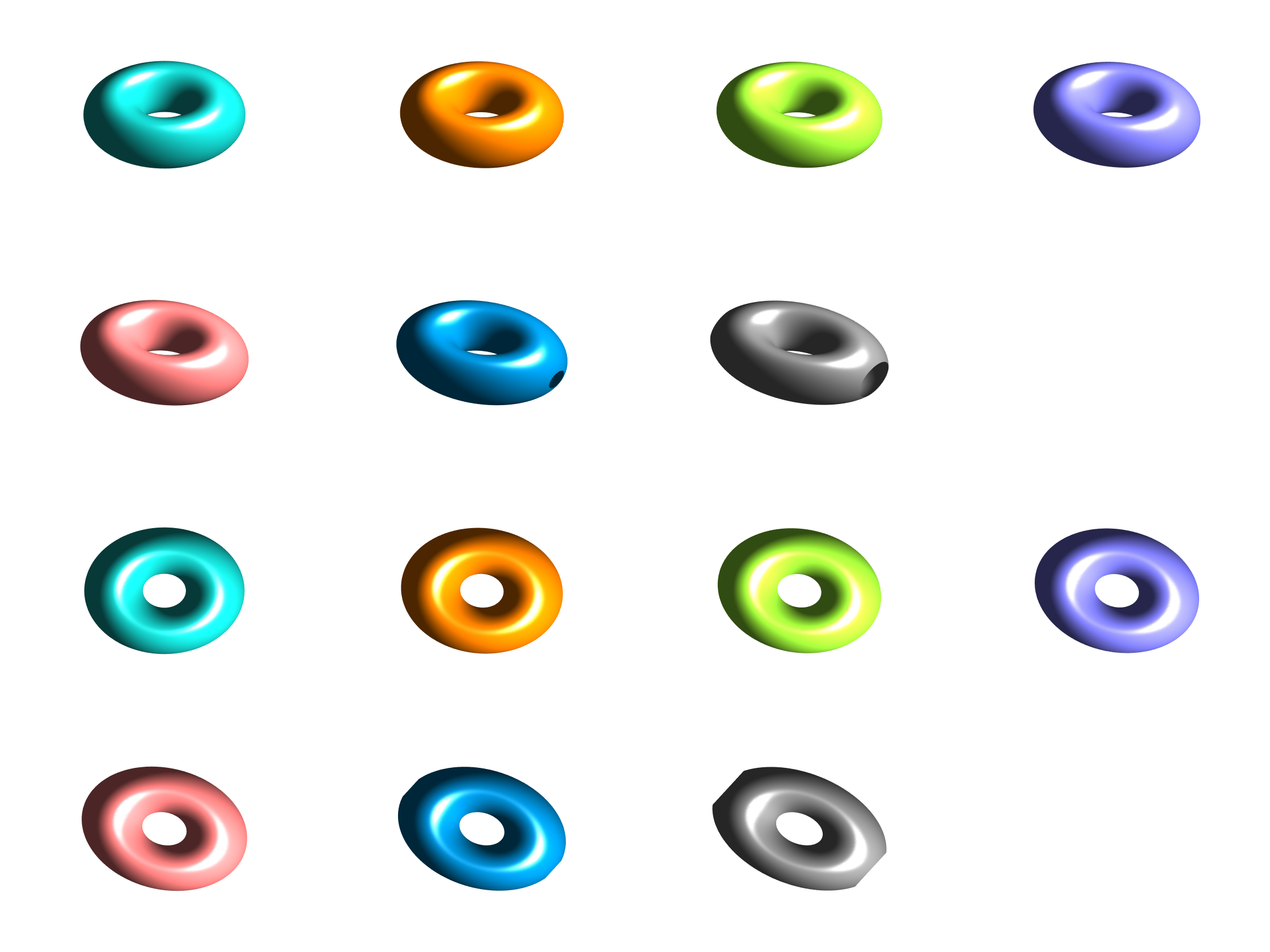
Figure 6: The first two rows and the last two rows present the same collection of seven surfaces from different angles. The seven surfaces in each collection represent the level set $\{x\in\mathbb{R}^{3}:\,h^{(\epsilon)}(x)=0.0834\}$ for seven indices $\epsilon\in\{0.7,\,0.8,\,0.85,\,0.875,\,0.9,\,0.95,\,1\}$, respectively.

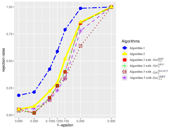
Figure 7: Rejection rates of Algorithms 1, 2, and 3 across different indices $\epsilon$. The verticle axis indicates the rejection rates across the 100 data replicates and the horizontal axis indicates $1-\epsilon$. In the figure, the label “Algorithm 3 with $\operatorname{dist}_{2,2}^{\operatorname{ERT}}$” refers to the implementation of Algorithm 3 where the input is $\operatorname{dist}=\operatorname{dist}_{2,2}^{\operatorname{ERT}}$. Analogously, labels with $\operatorname{dist}_{2,2}^{\operatorname{SERT}}$, $\operatorname{dist}_{2}^{\operatorname{SELECT}}$, and $\operatorname{dist}_{2}^{\operatorname{MEC}}$ function in the same manner.

8 Numerical Experiments

In this section, we show the performance of our proposed Algorithms 1, 2, and 3 using simulations. Specifically, we generate grayscale functions from a family of random fields and apply our proposed algorithms to them. Motivated by the simulation designs in Meng et al. (2022) and Kirveslahti and Mukherjee (2023), we apply Algorithms 1-3 to the following family of random grayscale functions

$$h^{(\epsilon)}(x_{1},x_{2},x_{3}):=\left\{\left(\sqrt{\frac{\alpha}{\epsilon}\cdot x_{1}^{2}+\epsilon\cdot\beta\cdot x_{2}^{2}}-\delta\right)^{2}+\gamma\cdot x_{3}^{2}\right\}\cdot\mathbbm{1}_{\{-1\leq x_{1},x_{2},x_{3}\leq 1\}},\ \ \ \text{ for }\epsilon\in[0.7,\,1].$$

where $\epsilon$ is a deterministic index, $\alpha,\beta,\gamma$ are iid $\operatorname{Unif}(0.5,1)$ random variables, $\delta\sim\operatorname{Unif}(0.4,0.6)$, and all the random variables are independent. Let $\mathbb{P}^{(\epsilon)}$ denote the underlying distribution corresponding to $h^{(\epsilon)}$. All the realizations of $h^{(\epsilon)}$ belong to $\mathfrak{D}_{R,d}$ with $R=2$ and $d=3$. The level sets $\{x\in\mathbb{R}^{3}:\,h^{(\epsilon)}(x)=0.0834\}$ for different indices $\epsilon\in\{0.7,\,0.8,\,0.85,\,0.875,\,0.9,\,0.95,\,1\}$ are presented in Figure 6.

Table 1: Rejection rates (RRs) of Algorithms 1, 2, and 3 across different indices $\varepsilon$. In the table, the label “Algorithm 3 with $\operatorname{dist}_{2,2}^{\operatorname{ERT}}$” refers to the implementation of Algorithm 3 where the input is $\operatorname{dist}=\operatorname{dist}_{2,2}^{\operatorname{ERT}}$. Analogously, labels with $\operatorname{dist}_{2,2}^{\operatorname{SERT}}$, $\operatorname{dist}_{2}^{\operatorname{SELECT}}$, and $\operatorname{dist}_{2}^{\operatorname{MEC}}$ function in the same manner.

	Null $\boldsymbol{H_{0}}$	Alternative $\boldsymbol{H_{1}}$
Indices $\boldsymbol{(1-\varepsilon)}$	0.000	0.050	0.100	0.125	0.150	0.200	0.300
RRs of Algorithm 1	0.18	0.21	0.43	0.59	0.79	0.99	1.00
RRs of Algorithm 2	0.05	0.08	0.22	0.30	0.52	0.86	1.00
RRs of Algorithm 3 with $\operatorname{dist}^{\operatorname{ERT}}_{2,2}$	0.05	0.02	0.16	0.27	0.40	0.86	1.00
RRs of Algorithm 3 with $\operatorname{dist}^{\operatorname{SERT}}_{2,2}$	0.05	0.06	0.14	0.23	0.34	0.78	1.00
RRs of Algorithm 3 with $\operatorname{dist}^{\operatorname{SELECT}}_{2}$	0.04	0.02	0.14	0.27	0.34	0.64	1.00
RRs of Algorithm 3 with $\operatorname{dist}^{\operatorname{MEC}}_{2}$	0.05	0.02	0.16	0.27	0.40	0.86	1.00

We apply our proposed algorithms to test the following hypotheses

$$H_{0}:\ \ \mathbb{P}{{}^{(1)}}=\mathbb{P}{{}^{(\epsilon)}}\ \ vs.\ \ H_{1}:\ \ \mathbb{P}{{}^{(1)}}\neq\mathbb{P}{{}^{(\epsilon)}}.$$ (8.1)

The null hypothesis $H_{0}$ in Eq. (8.1) is true if and only if $\epsilon=1$. We generate $n=30$ realizations of $h^{(1)}$. Then, for each $\epsilon\in[0.7,1]$, we generate $n=30$ realizations of $h^{(\epsilon)}$. We apply Algorithms 1, 2, and 3 to the two collections of generated grayscale functions to test the hypotheses in Eq. (8.1) with significance $0.05$ (i.e., the expected type I error rate is 0.05). We repeat this procedure 100 times, go through values of $\epsilon\in[0.7,1]$, and present the rejection rates across the 100 repetitions in Table 1 and Figure 7. The numerical experiment results can be summarized as follows:

1. Among all the algorithms, Algorithm 1 is the most powerful under the alternative hypothesis where $\epsilon\neq 1$. However, it suffers from type I error inflation — meaning that the expected rejection rate when $\epsilon=1$ is 0.05 but the rejection rate of Algorithm 1 is higher. As previously mentioned, the type I error inflation of Algorithm 1 stems from the numerical violation of Assumption 4.

2. Algorithm 2, which is a combination of the permutation technique and Algorithm 1, does not suffer from type I error inflation. While the power of Algorithm 2 is lower than that of Algorithm 1 under the alternative hypothesis, it is still uniformly more powerful than the full permutation test in Algorithm 3 with all the four distance inputs $\{\operatorname{dist}^{\operatorname{ERT}}_{2,2},\operatorname{dist}^{\operatorname{SERT}}_{2,2},\operatorname{dist}^{\operatorname{SELECT}}_{2},\operatorname{dist}^{\operatorname{MEC}}_{2}\}$.

3. The four distance inputs for Algorithm 3 result in comparable hypothesis testing performance. Particularly, the $\operatorname{dist}^{\operatorname{ERT}}_{2,2}$ and $\operatorname{dist}^{\operatorname{MEC}}_{2}$ result in the same performances when we apply them to Algorithm 3, which results from the similarity between the ERT and MEC. One theoretical advantage of the ERT over the MEC is that the ERT is homogeneous (i.e., $\operatorname{ERT}(\lambda\cdot g)=\lambda\cdot\operatorname{ERT}(g)$ for all $\lambda\in\mathbb{R}$).

The results described above are similar to those shown in Meng et al. (2022) for numerical experiments conducted on random binary images. Based on the experiment results concluded above, we recommend Algorithm 2 in applications for the following reason: it is uniformly powerful (compared with the fully permutation-based Algorithm 3) and does not suffer from type I error inflation.

9 Discussion

The ultimate goal of our study is to generalize a series of ECT-based methods (Crawford et al., 2020, Wang et al., 2021, Meng et al., 2022, Marsh et al., 2022) to the analysis of grayscale images. In this paper, we took an initial step towards this goal by proposing an ECT-like topological summary, the ERT. The framework proposed in Baryshnikov and Ghrist (2010) provides solid mathematical foundations for our proposed ERT. Building upon the ERT, we introduced the SERT as a generalization of the SECT (Crawford et al., 2020, Meng et al., 2022). Importantly, the SERT represents grayscale images as functional data. By applying the Karhunen–Loève expansion to the SERT, we have proposed effective statistical algorithms (see Algorithms 1-3) designed to detect significant differences between two sets of grayscale images. Particularly, Algorithm 2 was shown in simulations to be uniformly powerful while not suffering from type I error inflation.

There are many motivating questions for future research. A few of them from the biomedical perspective include:

1. Significantly different images usually correspond to different clinical outcomes (e.g., survival rates). Crawford et al. (2020) used the SECT on binary images of GBM tumors as the predictors in statistical inference. Here, the authors showed that the SECT has the power to predict clinical outcomes better than existing tumor quantification approaches. A natural generalization of the approach in Crawford et al. (2020) is the development of an SECT-like statistic designed for grayscale images which could prove to be powerful in terms of predicting clinical outcomes. For instance, one may consider analyzing the grayscale images in Figure 1 to predict the clinical outcomes of the corresponding lung cancer patients.

2. Suppose grayscale images can successfully predict a clinical outcome of interest. In that case, a subsequent question from the sub-image analysis viewpoint is: can we identify the physical features in the grayscales image that are most relevant to the clinical outcome? For binary images (equivalently, shapes), Wang et al. (2021) proposed an efficient method of seeking the desired physical features of shapes via the ECT. One may consider generalizing the method in Wang et al. (2021) to deal with grayscale images.

3. Tumors change over time. Hence, having the ability to study dynamically changing/longitudinal grayscale images is an area of interest. Using the ECT and SECT, Marsh et al. (2022) introduced the DETECT framework to analyze the dynamic changes in shapes. One may consider generalizing the DETECT approach to analyze the dynamic changes in grayscale images.

Lastly, another future direction would be to employ statistical methods analogous to those described in Section 7 for the analysis of networks using curvature-based approaches (Wu et al., 2022).

Software Availability

Code for implementing the Euler-Radon transform (ERT), the smooth Euler-Radon transform (SERT), as well as the lifted Euler characteristic transform (LECT) and the super lifted Euler characteristic transform (SELECT) is freely available at https://github.com/JinyuWang123/ERT.

Statements and Declarations

The authors declare no competing interests.

Appendix A Proofs

A.1 Proof of Eq. (3.9)

Proof.

For any $g\in\operatorname{CF}(X)$ and $n\in\mathbb{Z}$, we have $\lceil n\cdot g\rceil=n\cdot g=\lfloor n\cdot g\rfloor$. Hence,

$$\int_{X}g(x)\lceil\,d\chi(x)\rceil =\lim_{n\to\infty}\frac{1}{n}\int_{X}\lceil n\cdot g(x)\rceil\,d\chi(x)$$

$$=\lim_{n\to\infty}\frac{1}{n}\int_{X}n\cdot g(x)\,d\chi(x)$$

$$=\lim_{n\to\infty}\int_{X}g(x)\,d\chi(x)$$

$$=\int_{X}g(x)\,d\chi(x).$$

Similarly, we have that $\int_{X}g(x)\lfloor d\chi(x)\rfloor=\int_{X}g(x)d\chi(x)$. Therefore, we have $\int_{X}g(x)[d\chi(x)]=\int_{X}g(x)d\chi(x)$. Since $\mathbbm{1}_{K}\in\operatorname{CF}(X)$ for all $K\in\operatorname{CS}(X)$, we obtain Eq. (3.9). $\square$

A.2 Proof of Theorem 3.1

We need the following lemma in van den Dries (1998).

Lemma A.1 (rephrased “(2.10) Proposition,” Chapter 4 of van den Dries (1998)).

Let $S\subseteq\mathbb{R}^{m+d}$ be definable and $S_{a}:=\{x\in\mathbb{R}^{d}:\,(a,x)\in S\}$ for each $a\in\mathbb{R}^{m}$. Then, $\chi(S_{a})$ takes only finitely many values as $a$ runs through $\mathbb{R}^{m}$. Furthermore, for each integer $z$, the set $\{a\in\mathbb{R}^{m}:\,\chi(S_{a})=z\}$ is definable.

With Lemma A.1, we provide the proof of Theorem 3.1 as follows

Proof.

(Proof of Theorem 3.1.) We implement Lemma A.1 by defining the following

1. $m:=d+1$;

2. $a=(\nu,t)\in\mathbb{S}^{d-1}\times[0,T]\subseteq\mathbb{R}^{m}=\mathbb{R}^{d}\times\mathbb{R}$;

3. $S:=\left\{(\nu,t,x)\in\mathbb{R}^{d}\times\mathbb{R}\times\mathbb{R}^{d}:x\in K\text{ and }x\cdot\nu\leq t-R\right\}$. Since $S=\mathbb{R}^{d}\times\mathbb{R}\times K\cap\{(\nu,t,x)\in\mathbb{R}^{d}\times\mathbb{R}\times\mathbb{R}^{d}:\,x\cdot\nu-t+R\leq 0\}$, the set $S$ is definable under Assumption 1.

Then, for each fixed $a=(\nu,t)\in\mathbb{R}^{d}\times\mathbb{R}=\mathbb{R}^{m}$, we have

$$S_{a}=S_{(\nu,t)}=\{x\in K:\,x\cdot\nu\leq t-R\}=K_{t}^{\nu}.$$

Lemma A.1 implies that $\chi(S_{a})=\chi(K_{t}^{\nu})$ takes only finitely many values as $a=(\nu,t)$ runs through $\mathbb{R}^{m}=\mathbb{R}^{d}\times\mathbb{R}$. Therefore, $\chi(K_{t}^{\nu})$ takes only finitely many values as $(\nu,t)$ runs through $\mathbb{S}^{d-1}\times[0,T]$.

Furthermore, Lemma A.1 indicates that $\{(\nu,t)\in\mathbb{R}^{m}:\,\chi(K_{t}^{\nu})=z\}$ is definable for every integer $z$. Because $\mathbb{S}^{d-1}\times[0,T]$ is definable (under Assumption 1), we have that $\{(\nu,t)\in\mathbb{S}^{d-1}\times[0,T]:\,\chi(K_{t}^{\nu})=z\}=\mathbb{S}^{d-1}\times[0,T]\cap\{(\nu,t)\in\mathbb{R}^{m}:\,\chi(K_{t}^{\nu})=z\}$ is definable for every integer $z$. The proof of the first result of Theorem 3.1 is completed.

The second result is a straightforward corollary of the first. The third result of Theorem 3.1 is implied by the first result and the “monotonicity theorem” in Chapter 3 of van den Dries (1998). $\square$

A.3 Proof of Theorem 3.4

Proof.

It is straightforward that $\operatorname{ERT}(g)$ determines $\operatorname{SERT}(g)$. It suffices to show that $\operatorname{SERT}(g)$ determines $\operatorname{ERT}(g)$.

For every fixed direction $\nu\in\mathbb{S}^{d-1}$, the definition of $\operatorname{SERT}(g)$ implies

$$\frac{d}{dt}\operatorname{SERT}(g)(\nu,t)=\operatorname{ERT}(g)(\nu,t)+\left(-\frac{1}{T}\int_{0}^{T}\operatorname{ERT}(g)(\nu,\tau)\,d\tau\right),$$

for all $t\in[0,T]$ that are not discontinuities of $t\mapsto\operatorname{ERT}(g)(\nu,t)$. Recall that the support of $g$ is strictly smaller than the domain $B_{\mathbb{R}^{d}}(0,R)$. For any $t^{*}<\operatorname{dist}\left(\operatorname{supp}(g),\partial B_{\mathbb{R}^{d}}(0,R)\right)$, we have $g(x)\cdot R(x,\nu,t^{*})=0$ for all $x\in B_{\mathbb{R}^{d}}(0,R)$, which indicates that $\operatorname{ERT}(g)(\nu,t^{*})=\int_{B_{\mathbb{R}^{d}}(0,R)}g(x)\cdot R(x,\nu,t^{*})\,[d\chi(x)]=0$. Hence,

$$\lim_{t\rightarrow 0+}\frac{d}{dt}\operatorname{SERT}(g)(\nu,t)=-\frac{1}{T}\int_{0}^{T}\operatorname{ERT}(g)(\nu,\tau)\,d\tau,$$

which implies

$$\operatorname{ERT}(g)(\nu,t)=\frac{d}{dt}\operatorname{SERT}(g)(\nu,t)-\lim_{t\rightarrow 0+}\frac{d}{dt}\operatorname{SERT}(g)(\nu,t),$$ (A.1)

for all $t\in[0,T]$ that are not discontinuities of $t\rightarrow\operatorname{ERT}(g)(\nu,t)$. The right continuity of $t\mapsto\operatorname{ERT}(g)(\nu,t)$ implies that Eq. (A.1) holds for all $t\in[0,T]$. That is, $\operatorname{SERT}(g)$ determines $\operatorname{ERT}(g)$ through Eq. (A.1). The proof is completed. $\square$

A.4 Proof of Theorem 3.5

Before the proof of Theorem 3.5, we suggest the audiences read Appendix C, especially Proposition C.1, as a prerequisite for the proof. A takeaway message from Appendix C is that the ERT is invertible if the “Fubini condition” (Eq. (C.2)) is satisfied. In addition to Appendix C, we need the following lemma as a prerequisite

Lemma A.2.

If $f,g\in\operatorname{CF}(X)$, we have

$$\int_{X}\left\{a\cdot f(x)+b\cdot g(x)\right\}\,[d\chi(x)]=a\cdot\int_{X}f(x)\,d\chi(x)+b\cdot\int_{X}g(x)\,d\chi(x)$$

for all $a,b\in\mathbb{R}$.

Proof.

Both $a\cdot f(x)$ and $b\cdot g(x)$ are compactly supported real-valued definable functions; the images of $a\cdot f(x)$ and $b\cdot g(x)$ are both finite-point sets in $\mathbb{R}$. The equality above then follows from Lemma B.1 and the homogeneity of $[d\chi]$. $\square$

The following lemma implies the Fubini condition is satisfied by piecewise constant definable functions with compact support.

Lemma A.3.

Suppose $X$ is a definable set and $Y$ is a bounded subset of $\mathbb{R}^{N}$ for some positive integer $N$. If function $f\in\operatorname{Def}(X;\mathbb{R})$ takes finitely many values, we have the following

$$\int_{Y}\left(\int_{F^{-1}(y)}f(x)\,[d\chi(x)]\right)[d\chi(y)]=\int_{X}f(x)[d\chi(x)]$$

for all $F\in\operatorname{Def}(X;Y)$.

Proof.

Suppose $f$ takes values in $\{a_{i}\}_{i=1}^{m}$ with $m<\infty$. Denote $D_{i}:=\{x\in X:f(x)=a_{i}\}$ for $i=1,\ldots,m$ and $\mathcal{D}:=\{D_{i}\}_{i=1}^{m}$. By the “cell decomposition theorem” (see Chapter 3 of van den Dries (1998)), there exists a finite decomposition $\mathcal{E}$ of $X$ such that, for each $E\in\mathcal{E}$, the restriction $F|_{E}$ is continuous. Denote $\mathcal{G}:=\{D\cap E:\,D\in\mathcal{D}\text{ and }E\in\mathcal{E}\}=:\{G_{i}\}_{i=1}^{n}$; obviously, $\mathcal{G}$ is a finite definable partition of $X$. Furthermore, for every component $G_{i}\in\mathcal{G}$, $F$ is continuous on $G_{i}\in\mathcal{G}$ and $f$ is a constant (say $b_{i}$) on $G_{i}$.

For each $i=1,\ldots,n$, define the restriction $F_{i}:=F|_{G_{i}}:G_{i}\to Y$. Since $F_{i}$ is continuous on $G_{i}$, the “trivialization theorem” (see Chapter 9 of van den Dries (1998)) implies that there exists a finite definable partition $\{Y_{ij}\}_{j}$ of $Y$ such that $F_{i}$ is definably trivial over $Y_{ij}$ for each $j$. That is, for each $j$, there exists a definable set $U_{ij}\subseteq\mathbb{R}^{N}$ for some $N$ and a definable map $\lambda_{ij}:F_{i}^{-1}(Y_{ij})\rightarrow U_{ij}$ such that $h_{ij}:=(F_{i}|_{F_{i}^{-1}(Y_{ij})},\,\lambda_{ij}):F_{i}^{-1}(Y_{ij})\rightarrow Y_{ij}\times U_{ij}$ is a homeomorphism; furthermore, $F_{i}|_{F_{i}^{-1}(Y_{ij})}=\pi\circ h_{ij}$, where $\pi:Y_{ij}\times U_{ij}\rightarrow Y_{ij}$ is a projection map, and $F_{i}^{-1}(y)$ is definably homeomorphic to $U_{ij}$ for each $y\in Y_{ij}$.

The additivity of Euler characteristics implies

$$\int_{Y}\left(\int_{F^{-1}(y)}f(x)\,[d\chi(x)]\right)[d\chi(y)] =\int_{Y}\sum_{i=1}^{n}\left(\int_{F_{i}^{-1}(y)}f(x)\,[d\chi(x)]\right)[d\chi(y)]$$

$$=\int_{Y}\sum_{i=1}^{n}b_{i}\cdot\chi\left(F_{i}^{-1}(y)\right)[d\chi(y)]$$

Lemma A.1 implies that $y\mapsto\chi(F_{i}^{-1}(y))=\chi(\{x\in X:F_{i}(x)=y\})$ is a constructible function defined on $Y$. Therefore, Lemma A.2, together with the additivity of Euler characteristics, implies the following

$$\int_{Y}\left(\int_{F^{-1}(y)}f(x)\,[d\chi(x)]\right)[d\chi(y)] =\sum_{i=1}^{n}b_{i}\int_{Y}\chi\left(F_{i}^{-1}(y)\right)d\chi(y)$$

$$=\sum_{i=1}^{n}b_{i}\sum_{j}\int_{Y_{ij}}\chi\left(F_{i}^{-1}(y)\right)d\chi(y)$$

Since all fibers $F_{i}^{-1}(y)$ for $y\in Y_{ij}$ are all definably homeomorphic to $U_{ij}$, we have $\chi\left(F_{i}^{-1}(y)\right)=\chi(U_{ij})$ for all $y\in Y_{ij}$. Hence, we have

$$\int_{Y}\left(\int_{F^{-1}(y)}f(x)\,[d\chi(x)]\right)[d\chi(y)] =\sum_{i=1}^{n}b_{i}\sum_{j}\int_{Y_{ij}}\chi(U_{ij})\,[d\chi(y)]$$

$$=\sum_{i=1}^{n}b_{i}\sum_{j}\chi(Y_{ij})\cdot\chi(U_{ij})$$

$$=\sum_{i=1}^{n}b_{i}\sum_{j}\chi(Y_{ij}\times U_{ij})$$

$$=\sum_{i=1}^{n}b_{i}\sum_{j}\chi\left(F_{i}^{-1}(Y_{ij})\right).$$

Since, for each $i$, $\{Y_{ij}\}_{j}$ is a partition of $Y$, we have

$$\int_{Y}\left(\int_{F^{-1}(y)}f(x)\,[d\chi(x)]\right)[d\chi(y)] =\sum_{i=1}^{n}b_{i}\chi\left(F_{i}^{-1}(Y)\right)$$

$$=\sum_{i=1}^{n}b_{i}\chi\left(G_{i}\right)$$

$$=\sum_{i=1}^{n}b_{i}\int_{X}\mathbbm{1}_{G_{i}}(x)\,d\chi(x).$$

Applying Lemma A.2 again, we have

$$\int_{Y}\left(\int_{F^{-1}(y)}f(x)\,[d\chi(x)]\right)[d\chi(y)] =\int_{X}\sum_{i=1}^{n}b_{i}\cdot\mathbbm{1}_{G_{i}}(x)\,[d\chi(x)]$$

$$=\int_{X}f(x)\,[d\chi(x)]$$

This concludes the proof. $\square$

Proof of Theorem 3.5.

Our goal is to prove that Eq. (C.2) is true if $g\in\mathfrak{D}_{R,d}^{pc}$, which implies the desired invertibility via Proposition C.1.

For the ease of notations, we will denote $S=B_{\mathbb{R}^{d}}(0,R)$ and $T=\mathbb{S}^{d-1}\times[0,T]$. Let $x^{\prime}$ be any point in $S$ and fixed. The kernel functions $R(x,\nu,t)$ and $R^{\prime}(\nu,t,x^{\prime})$ are defined in Eq. (3.1) and Eq. (3.14), respectively. Let $g\in\mathfrak{D}_{R,d}^{pc}$. Then, the function $(x,\nu,t)\mapsto g(x)\cdot R(x,\nu,t)\cdot R^{\prime}(\nu,t,x^{\prime})$ belongs to $\operatorname{Def}(S\times T;\mathbb{R})$ and takes finitely many values. Consider the standard projection maps $p_{1}:S\times T\to S$ and $p_{2}:S\times T\to T$ as follows

1. Applying Lemma A.3 to $p_{1}$, we have the following

   $$\int_{S\times T}g(x)\cdot R(x,\nu,t)\cdot R^{\prime}(\nu,t,x^{\prime})\,[d\chi(x,\nu,t)]$$

   $$=\int_{S}\left(\int_{p_{1}^{-1}(x)}g(x)\cdot R(x,\nu,t)\cdot R^{\prime}(\nu,t,x^{\prime})\,[d\chi(x,\nu,t)]\right)[d\chi(x)]$$

   $$=\int_{S}\left(\int_{\{x\}\times T}g(x)\cdot R(x,\nu,t)\cdot R^{\prime}(\nu,t,x^{\prime})\,[d\chi(x,\nu,t)]\right)[d\chi(x)]$$

   $$=\int_{S}g(x)\left(\int_{T}R(x,\nu,t)\cdot R^{\prime}(\nu,t,x^{\prime})\,[d\chi(\nu,t)]\right)[d\chi(x)].$$

2. Applying Lemma A.3 to $p_{2}$, we have the following

   $$\int_{S\times T}g(x)\cdot R(x,\nu,t)\cdot R^{\prime}(\nu,t,x^{\prime})\,[d\chi(x,\nu,t)]$$

   $$=\int_{T}\left(\int_{p_{2}^{-1}(\nu,t)}g(x)\cdot R(x,\nu,t)\cdot R^{\prime}(\nu,t,x^{\prime})\,[d\chi(x,\nu,t)]\right)[d\chi(\nu,t)]$$

   $$=\int_{T}\left(\int_{S\times\{(\nu,t)\}}g(x)\cdot R(x,\nu,t)\cdot R^{\prime}(\nu,t,x^{\prime})\,[d\chi(x,\nu,t)]\right)[d\chi(\nu,t)]$$

   $$=\int_{T}\left(\int_{S}g(x)\cdot R(x,\nu,t)\cdot R^{\prime}(\nu,t,x^{\prime})\,[d\chi(x)]\right)[d\chi(\nu,t)]$$

   $$=\int_{T}\left(\int_{S}g(x)\cdot R(x,\nu,t)\,[d\chi(x)]\right)R^{\prime}(\nu,t,x^{\prime})\,[d\chi(\nu,t)].$$

Combining the two equations above gives the desired Eq. (C.2).

Lastly, the invertibility of the SERT follows from Theorem 3.4. The proof is completed. $\square$

A.5 Proof of Theorem 4.2

Proof.

Denote $S_{\nu,t}:=B_{\mathbb{R}^{d}}(0,R)\cap\{x\in\mathbb{R}^{d}:x\cdot\nu\leq t-R\}$. A direct computation shows that

$$\int_{\mathbb{R}}s\cdot\operatorname{LECT}(g)(\nu,t,s)\,[d\chi(s)] =\int_{\mathbb{R}}s\cdot\chi\left(\left\{x\in B_{\mathbb{R}^{d}}(0,R):\,x\cdot\nu\leq t-R\text{ and }g(x)=s\right\}\right)\,[d\chi(s)]$$

$$=\int_{\mathbb{R}}s\cdot\chi\left(\left\{x\in S_{\nu,t}:g(x)=s\right\}\right)\,[d\chi(s)].$$

“Corollary 8” of Baryshnikov and Ghrist (2010) implies the following

$$\int_{\mathbb{R}}s\cdot\chi\left(\left\{x\in S_{\nu,t}:g(x)=s\right\}\right)\,[d\chi(s)] =\int_{S_{\nu,t}}g(x)\,[d\chi(x)]$$

$$=\int_{B_{\mathbb{R}^{d}}(0,R)}g(x)\cdot R(x,\nu,t)\,[d\chi(x)]$$

$$=\operatorname{ERT}(g)(\nu,t).$$

Then, Eq. (4.4) follows.

We can write “Proposition 2” of Baryshnikov and Ghrist (2010) using the LECT and SELECT as follows

$$\lfloor\operatorname{ERT}\rfloor(g)(\nu,t) =\int_{B_{\mathbb{R}^{d}}(0,R)}g(x)\cdot R(x,\nu,t)\,\lfloor d\chi(x)\rfloor$$

$$=\int_{S_{\nu,t}}g(x)\,\lfloor d\chi(x)\rfloor$$

$$=\int_{0}^{\infty}\operatorname{SELECT}(g)(\nu,t,s)-\operatorname{SELECT}(-g)(\nu,t,s)+\operatorname{LECT}(-g)(\nu,t,s)\,ds.$$

Similarly, we have

$$\lceil\operatorname{ERT}\rceil(g)(\nu,t)=\int_{0}^{\infty}\operatorname{SELECT}(g)(\nu,t,s)-\operatorname{LECT}(g)(\nu,t,s)-\operatorname{SELECT}(-g)(\nu,t,s)\,ds.$$

Thus, the proof of Eq. (4.5) is completed. Taking the average of the two expressions in Eq. (4.5) gives Eq. (4.6). $\square$

Appendix B Definability vs. Tameness of Functions

In the literature on TDA, one may often come across the concept of tameness. The word “tame” is also often used interchangeably with “definable.” The concept of definability is presented in Definition 3.2, and the concept of tameness can be found in Bobrowski and Borman (2012). In this section, we analyze the relationship between them. To avoid confusion, we will not interchange the words “definable” and “tame” in this paper.

B.1 Tameness

We first go through the concept of tameness as follows, which is a generalized version of “Definition 2.2” in Bobrowski and Borman (2012).

Definition B.1.

Let $X$ be a topological space with finite $\chi(X)$ and $f:X\to\mathbb{R}$ a continuous bounded function. For each $\alpha\in\mathbb{R}$, we define the super-level set at $\alpha$ as $X_{\alpha^{+}}^{f}\coloneqq\{x\in X:\ f(x)\geq\alpha\}$ and the sub-level set $\alpha$ $X_{\alpha^{-}}^{f}\coloneqq\{x\in X:\ f(x)\leq\alpha\}$. The function $f$ is said to be tame if it satisfies the following two conditions

• The homotopy types of $X_{\alpha^{+}}^{f}$ and $X_{\alpha^{-}}^{f}$ change finitely many times as $\alpha$ varies through $\mathbb{R}$;

• the homology groups of $X_{\alpha^{+}}^{f}$ and $X_{\alpha^{-}}^{f}$ are all finitely generated for all $\alpha\in\mathbb{R}$.

Similar to Definition B.1, we define the following

Definition B.2.

Let $X$ be a topological space with finite $\chi(X)$. A (not necessarily continuous) bounded function $f:X\to\mathbb{R}$ is said to be EC-tame if the Euler characteristics $\chi(X_{\alpha^{+}}^{f})$ and $\chi(X_{\alpha^{-}}^{f})$ are finite for all $\alpha\in\mathbb{R}$ and change only finitely many times as $\alpha$ varies through $\mathbb{R}$.

Note that the definition of “tame functions” in Bobrowski and Borman (2012) are equivalent to continuous EC-tame functions on compact topological space $X$ in our context.

B.2 Relationship between Tameness and Definability

In general, it is not the case that a tame function is definable in the o-minimal sense, which is illustrated by the following example.

Example B.1.

Let $W$ denote the Warsaw circle (see Figure 8) defined as the union of the closed topologist’s sine curve and an arc $J$ “joining” the two ends of the topologist’s sine curve:

$$W\coloneqq\{(x,\sin(\frac{2\pi}{x})\ |\ x\in(0,1]\}\cup\{(0,y)\ |\ -1\leq y\leq 1\}\cup J$$

$$J\coloneqq\{(0.5+R\cos(t),-2+R\sin(t)\ |\ \beta\leq t\leq 2\pi+\alpha\}\}$$

$$R\coloneqq\sqrt{(\frac{1}{2})^{2}+2^{2}},\alpha\coloneqq\arctan(\frac{2}{0.5}),\beta=\pi-\alpha$$

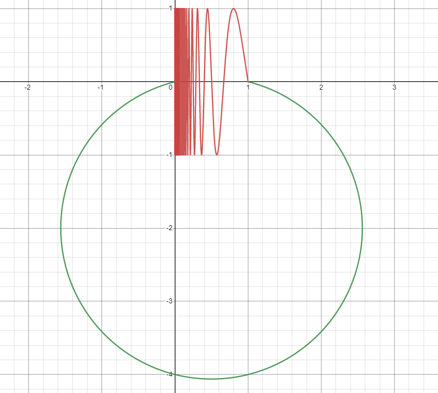
Figure 8: The Warsaw Circle $W$

$W$ itself is not definable. However, $W$ is compact as it is bounded and is the union of two closed sets (the closed topologist’s sine curve and $J$). Now consider the constant continuous function $f:W\to\mathbb{R}$ that sends every point to $0$ - the graph of this function is $W\times\{0\}\subseteq\mathbb{R}^{3}$ and is not definable. Hence, $f$ is not definable.

On the other hand, the function is a tame function. This is because the Warsaw Circle is known to be simply connected and has all trivial homology groups beyond dimension $0$.

Remark B.1.

If $f:X\to Y$ is a tame function between two definable sets, would $f$ be definable? The answer is no. Consider the indicator function $\mathbbm{1}_{W}:\mathbb{R}^{2}\to\mathbb{R}$ on the Warsaw circle $W$.

Conversely, a function that is definable in the o-minimal sense does not have to be tame either. The most obvious obstruction comes from the distinction that definable functions need not be continuous nor bounded. However, when we remove the trivial distinctions between the two, we do have the following result:

Proposition B.1.

Suppose $X\subseteq\mathbb{R}^{n}$ is definable. If the function $f:X\to\mathbb{R}$ is continuous, bounded, and definable, then $f$ is tame.

Proof.

Let $\Gamma(f)\subset X\times\mathbb{R}$ be the graph of $f$ and let $\pi:\mathbb{R}^{n}\times\mathbb{R}\to\mathbb{R}^{n}$ be the standard projection function, we observe that $X_{\alpha^{+}}^{f}$ is the set $\pi(\Gamma(f)\cap X\times[\alpha,+\infty))$ and is thus definable.

By the triangulation theorem (see Chapter 8 of van den Dries (1998)), it follows that $X_{\alpha^{+}}^{f}$ is definably homeomorphic to a subcollection of open simplices in some finite Euclidean simplicial complex, which implies that the homology groups of $X_{\alpha^{+}}^{f}$ are all finitely generated. The case for $X_{\alpha^{-}}^{f}$ is similar.

Since $f:X\to\mathbb{R}$ is a continuous definable function between definable sets, the “trivialization theorem” (see Chapter 9 of van den Dries (1998)) asserts that there exists a definable partition of $\mathbb{R}$ into finitely many definable sets $R_{1},...,R_{n}$ such that, for any $i\in\{1,...,n\}$, there exists a definable set $Y_{i}\subseteq\mathbb{R}^{N}$, for some dimension $N$, making the following diagram commute

where $f_{i}$ is the function $f$ restricted to $f^{-1}(R_{i})$ with $f_{i}:=f|_{f^{-1}(R_{i})}$, $h_{i}$ is a homeomorphism, $\lambda_{i}:f^{-1}(R_{i})\rightarrow Y_{i}$ is a continuous map, and $\pi_{i}:R_{i}\times Y_{i}\rightarrow R_{i}$ is the standard projection map.

It is straightforward to have the following disjoint union

$$\begin{aligned} X_{\alpha^{+}}^{f}&=\{x\in X:\ f(x)\geq\alpha\}\\ &=\bigcup_{i=1}^{n}\left\{x\in f^{-1}(R_{i}):\,f_{i}(x)\geq\alpha\right\}\\ &=\bigcup_{i=1}^{n}\left\{x\in f^{-1}(R_{i}):\,\pi_{i}\circ h_{i}(x)\geq\alpha\right\}\\ &=\bigcup_{i=1}^{n}\left\{\xi\in h_{i}\left(f^{-1}(R_{i})\right):\,\pi_{i}(\xi)\geq\alpha\right\}\\ &=\bigcup_{i=1}^{n}\left\{\xi\in R_{i}\times Y_{i}:\,\pi_{i}(\xi)\geq\alpha\right\}.\end{aligned}$$ (B.1)

To show that the homotopy type of $X_{\alpha^{+}}^{f}$ changes finitely many times, Eq. (B.1) indicates that it suffices to verify that, for each projection map $\pi_{i}$, the homotopy type of the super-level sets of $\pi_{i}$ changes finitely many times. Indeed, since $R_{i}\in\mathcal{O}_{1}$, the set $R_{i}$ is a finite union of points and open intervals. The homotopy type of $\left\{\xi\in R_{i}\times Y_{i}:\,\pi_{i}(\xi)\geq\alpha\right\}$ changes only when $\alpha$ crosses the isolated points and boundary points of $R_{i}$. The verification for the sub-level sets is similar. Hence, $f$ is a tame function. $\square$

B.3 A Useful Formula

We use Proposition B.1 to prove a variant of “Proposition 7.2” in Bobrowski and Borman (2012), which will be implemented in Appendix C.

Lemma B.1.

Suppose the topological space $X$ is definable, and functions $h,f:X\to\mathbb{R}$ are definable. If the image of $h$ is discrete and $f$ is bounded, then we have the following formula

$$\int_{X}(h+f)\lceil d\chi\rceil=\int_{X}h\lceil d\chi\rceil+\int_{X}f\lceil d\chi\rceil$$

The formula holds similarly for $\lfloor d\chi\rfloor$.

Proof.

Since $h(X)$ belongs to $\mathcal{O}_{1}$ and is discrete, $h(X)$ must be a finite point set, say $\{a_{1},...,a_{n}\}$. We can then partition $X$ into $A_{1},...,A_{n}$ such that

$$h(x)=\sum_{i=1}^{n}a_{i}\mathbbm{1}_{A_{i}}(x).$$

In addition, the “cell decomposition theorem” (see Chapter 3 of van den Dries (1998)) indicates that there exists a cell decomposition $\mathcal{D}$ of $X$ such that $f$ is continuous on each cell in $\mathcal{D}$. Hence, without loss of generality, we may assume that $f$ is continuous on each $A_{i}$.

By additivity of Euler characteristics, we can decompose $\int_{X}(h+f)\lceil d\chi\rceil$ as follows

$$\int_{X}(h+f)\lceil d\chi\rceil =\int_{X}\sum_{i=1}^{n}(a_{i}+f)\cdot\mathbbm{1}_{A_{i}}\lceil d\chi\rceil$$

$$=\lim_{k\rightarrow\infty}\frac{1}{k}\int_{X}\left\lceil\sum_{i=1}^{n}k\cdot(a_{i}+f)\cdot\mathbbm{1}_{A_{i}}\right\rceil\,d\chi$$

$$=\lim_{k\rightarrow\infty}\frac{1}{k}\int_{X}\sum_{i=1}^{n}\left\lceil k\cdot(a_{i}+f)\right\rceil\cdot\mathbbm{1}_{A_{i}}\,d\chi$$

$$=\lim_{k\rightarrow\infty}\frac{1}{k}\sum_{i=1}^{n}\int_{X}\left\lceil k\cdot(a_{i}+f)\right\rceil\cdot\mathbbm{1}_{A_{i}}\,d\chi$$

$$=\sum_{i=1}^{n}\lim_{k\rightarrow\infty}\frac{1}{k}\int_{A_{i}}\left\lceil k\cdot(a_{i}+f)\right\rceil\,d\chi$$

$$=\sum_{i=1}^{n}\int_{A_{i}}(a_{i}+f)\lceil d\chi\rceil.$$

It then suffices to verify $\int_{A_{i}}a_{i}+f\lceil d\chi\rceil=\int_{A_{i}}f\lceil d\chi\rceil+\int_{A_{i}}a_{i}\lceil d\chi\rceil$. Since $a_{i}+f$ is continuous on $A_{i}$ for each $i$, Proposition B.1 implies that $(a_{i}+f)|_{A_{i}}$ is tame. Then, it follows from “Proposition 2.4” of Bobrowski and Borman (2012) that

$$\int_{A_{i}}(a_{i}+f)\,\lceil d\chi\rceil =\sum_{v\in\operatorname*{CV}(a_{i}+f)}\Delta_{\chi}(a_{i}+f,v)v$$

$$=\sum_{v\in\operatorname*{CV}(f)}\Delta_{\chi}(f,v)(v+a_{i})$$

$$=\sum_{v\in\operatorname*{CV}(f)}\Delta_{\chi}(f,v)v+a_{i}\sum_{v\in\operatorname*{CV}(f)}\Delta_{\chi}(f,v)$$

$$=\int_{A_{i}}f\lceil d\chi\rceil+a_{i}\sum_{v\in\operatorname*{CV}(f)}\Delta_{\chi}(f,v)$$

where $\operatorname*{CV}(f)$ is the set of values $\alpha$ (referred to as critical values) at which the homotopy type of $\{x\in A_{i}:\,f(x)\leq\alpha\}$ changes; and $\Delta_{\chi}(f,v)$ is the change in Euler characteristic:

$$\Delta_{\chi}(f,v)=\chi(\{x\in A_{i}:\,f(x)\leq v+\varepsilon\})-\chi(\{x\in A_{i}:\,f(x)\leq v-\varepsilon\})$$ (B.2)

for sufficiently small $\varepsilon$.

Since $f$ is bounded, so there exists $a\leq b$ such that $\{x\in A_{i}:\,f(x)\leq b\}=X$ and $\{x\in A_{i}:\,f(x)\leq a\}=\emptyset$. The sum $\sum_{v\in\operatorname*{CV}(f)}\Delta_{\chi}(f,v)$ then collapse as a telescoping sum to $\chi(A_{i})-\chi(\emptyset)=\chi(A_{i})$ (see Eq. (B.2)), hence

$$\int_{A_{i}}a_{i}+f\lceil d\chi\rceil=\int_{A_{i}}f\lceil d\chi\rceil+a_{i}\chi(A_{i})=\int_{A_{i}}f\lceil d\chi\rceil+\int_{A_{i}}a_{i}\lceil d\chi\rceil$$

The proof is completed. $\square$

Appendix C Discussions on the Invertibility of the ERT

In this section, we discuss the invertibility of the ERT, especially its dependence on the “Fubini condition.” This section provides a prerequisite for the proof of Theorem 3.5.

Let $\mu=1-(-1)^{d}$ and $\lambda=1$. Schapira (1995) and the proof of “Theorem 5” in Ghrist et al. (2018) show the following

$$\int_{\mathbb{S}^{d-1}\times[0,T]}R(x,\nu,t)\cdot R^{\prime}(\nu,t,x^{\prime})\,d\chi(\nu,t)=(\mu-\lambda)\delta_{\Delta}(x,x^{\prime})+\lambda,$$ (C.1)

where $R^{\prime}(\nu,t,x^{\prime})$ is the dual kernel defined in Eq. (3.14), and $\delta_{\Delta}(x,x^{\prime})=1$ if $x=x^{\prime}$ and is $0$ otherwise.

We recall the dual Euler-Radon transform (DERT) in Equation 3.15 as follows

$$\begin{aligned} \operatorname{DERT}:\ \ &\operatorname{Def}(\mathbb{S}^{d-1}\times[0,T])\rightarrow\mathbb{R}^{B_{\mathbb{R}^{d}}(0,R)},\\ &h\mapsto\operatorname{DERT}(h)=\left\{\operatorname{DERT}(h)(x):=\int_{\mathbb{S}^{d-1}\times[0,T]}h(\nu,t)\cdot R^{\prime}(\nu,t,x)\,[d\chi(\nu,t)]\right\}_{x\in B_{\mathbb{R}^{d}}(0,R)}.\end{aligned}$$

The following proposition shows the relationship between the ERT and DERT, which is the core of the proof of Theorem 3.5.

Proposition C.1.

Suppose $g\in\mathfrak{D}_{R,d}$. If the following condition (referred to as the “Fubini condition” hereafter) holds

$$\begin{aligned} &\int_{\mathbb{S}^{d-1}\times[0,T]}\left(\int_{B_{\mathbb{R}^{d}}(0,R)}g(x)\cdot R(x,\nu,t)[d\chi(x)]\right)R^{\prime}(\nu,t,x^{\prime})[d\chi(v,t)]\\ &=\int_{B_{\mathbb{R}^{d}}(0,R)}g(x)\left(\int_{\mathbb{S}^{d-1}\times[0,T]}R(x,\nu,t)\cdot R^{\prime}(\nu,t,x^{\prime})\,d\chi(\nu,t)\right)[d\chi(x)],\end{aligned}$$ (C.2)

we have the following formula

$$(\operatorname{DERT}\circ\operatorname{ERT})(g)(x^{\prime})=(\mu-\lambda)\cdot g(x^{\prime})+\lambda\left(\int_{B_{\mathbb{R}^{d}}(0,R)}g[d\chi]\right),\ \ \ \text{for all }x^{\prime}\in B_{\mathbb{R}^{d}}(0,R),$$ (C.3)

where $\mu=1-(-1)^{d}$ and $\lambda=1$.

Before providing the proof of Proposition C.1, we explain how Eq. (C.3) implies the invertibility of the ERT. Since $g$ has compact support, we have $\lim_{\xi\rightarrow R\mathbb{S}^{d-1}}g(\xi)=0$, where $\lim_{\xi\rightarrow R\mathbb{S}^{d-1}}$ means that $\xi$ converges to a point on the sphere $R\mathbb{S}^{d-1}=\{x\in\mathbb{R}^{d}:\,\|x\|=R\}$. Therefore, we have

$$\lim_{\xi\rightarrow R\mathbb{S}^{d-1}}\frac{1}{\mu-\lambda}\cdot(\operatorname{DERT}\circ\operatorname{ERT})(g)(\xi)=\lim_{\xi\rightarrow R\mathbb{S}^{d-1}}g(\xi)+\frac{\lambda}{\mu-\lambda}\left(\int_{B_{\mathbb{R}^{d}}(0,R)}g[d\chi]\right)=\frac{\lambda}{\mu-\lambda}\left(\int_{B_{\mathbb{R}^{d}}(0,R)}g[d\chi]\right).$$

The limit above implies

$$g(x^{\prime})=\frac{1}{\mu-\lambda}\cdot(\operatorname{DERT}\circ\operatorname{ERT})(g)(x^{\prime})-\lim_{\xi\rightarrow R\mathbb{S}^{d-1}}\frac{1}{\mu-\lambda}\cdot(\operatorname{DERT}\circ\operatorname{ERT})(g)(\xi),$$

which is the inversion formula in Eq. (3.16) and shows the invertibility of the ERT.

We provide the proof of Proposition C.1 as follows

Proof of Proposition C.1.

For ease of notation, let $X=B_{\mathbb{R}^{d}}(0,R)$ and $Y=\mathbb{S}^{d-1}\times[0,T]$. Then, we have

$$\left(\operatorname{DERT}\circ\operatorname{ERT}\right)(g)(x^{\prime}) =\operatorname{DERT}\left(\int_{X}g(x)\cdot R(x,\cdot,\cdot)\,[d\chi(x)]\right)(x^{\prime})$$

$$=\int_{Y}\left(\int_{X}g(x)\cdot R(x,\nu,t)[d\chi(x)]\right)R^{\prime}(\nu,t,x^{\prime})\,[d\chi(\nu,t)].$$

The Fubini condition in Eq. (C.2) implies

$$\left(\operatorname{DERT}\circ\operatorname{ERT}\right)(g)(x^{\prime}) =\int_{X}g(x)\left(\int_{Y}R(x,\nu,t)R^{\prime}(\nu,t,x^{\prime})[d\chi(\nu,t)]\right)\,[d\chi(x)].$$

Eq. (C.1) indicates the following

$$\left(\operatorname{DERT}\circ\operatorname{ERT}\right)(g)(x^{\prime}) =\int_{X}g(x)\left\{(\mu-\lambda)\delta_{\Delta}(x,x^{\prime})+\lambda\right\}\,[d\chi(x)]$$

$$=\int_{X}(\mu-\lambda)\cdot g(x)\cdot\delta_{\Delta}(x,x^{\prime})+\lambda\cdot g(x)\,[d\chi(x)]$$

For each fixed $x^{\prime}$, the function $(\mu-\lambda)g(x)\delta_{\Delta}(x,x^{\prime})$ of $x$ is clearly discrete. Then, Lemma B.1 implies

$$\left(\operatorname{DERT}\circ\operatorname{ERT}\right)(g)(x^{\prime})=\int_{X}(\mu-\lambda)g(x)\delta_{\Delta}(x,x^{\prime})[d\chi(x)]+\int_{X}\lambda g(x)[d\chi(x)].$$

Evaluating the two integrals above and keeping in mind that $\int(\cdot)[d\chi(x)]$ is homogeneous, we have that

$$(\operatorname{DERT}\circ\operatorname{ERT})(h)(x^{\prime})=(\mu-\lambda)g(x^{\prime})+\lambda\left(\int_{B_{\mathbb{R}^{d}}(0,R)}g[d\chi]\right),$$

that is, the proof of Eq. (C.3) is completed. $\square$

The Fubini condition specified above does fail in general. Plenty of examples are given in “Corollary 6” of Baryshnikov and Ghrist (2010). In “Theorem 7” of Baryshnikov and Ghrist (2010), this condition does hold when the definable function preserves fibers, ie. if $F:X\to Y$ is definable and $h\in\operatorname*{Def}(X,\mathbb{R})$ is constant on the fibers of $F$, then

$$\int_{X}h[d\chi(x)]=\int_{Y}\left(\int_{F^{-1}(y)}h(x)[d\chi(x)]\right)[d\chi(y)]$$

Unfortunately, this does not help much in the discussion of invertibility. The typical Fubini’s Theorem for $d\chi$ that swaps the order of integration

$$\int_{X}\int_{Y}f(x,y)d\chi(y)d\chi(x)=\int_{Y}\int_{X}f(x,y)d\chi(x)d\chi(y)$$

is a consequence of choosing $F$ to be the projection maps $p_{X}:X\times Y\to X$ and $p_{Y}:X\times Y\to Y$. However, if we additionally impose the constraint that $f$ is constant on the fibers of $p_{X}$ and $p_{Y}$, this is the same as requiring $f$ to be identically constant on $X\times Y$.

Appendix D Discussion on $\lim_{\sigma\rightarrow 0}\operatorname{ERT}(\phi_{\sigma}*\mathbbm{1}_{K})$

Let $\phi_{\sigma}$ be a kernel function with a bandwidth $\sigma$ (e.g., see Eq. (D.1)), and $\phi_{\sigma}*\mathbbm{1}_{K}$ the convolution of two functions. Although $\lim_{\sigma\rightarrow 0}\phi_{\sigma}*\mathbbm{1}_{K}(x)=\mathbbm{1}_{K}(x)$ almost everywhere (e.g., see “Theorem 4.1” of Stein and Shakarchi (2011)), it is not generally true that $\lim_{\sigma\rightarrow 0}\operatorname{ERT}(\phi_{\sigma}*\mathbbm{1}_{K})=\operatorname{ERT}(\mathbbm{1}_{K})=\operatorname{ECT}(K)$. This phenomenon is symbolic of the general principle that a set of Lebesgue measure zero may not be of Euler characteristic zero.

Let $\phi_{\sigma}$ be a kernel function with a bandwidth $\sigma$. For example

$$\begin{aligned} &\phi_{\sigma}(x)=\begin{cases}\frac{C_{d}}{\sigma^{d}}\cdot\exp\left(-\frac{\sigma^{2}}{\sigma^{2}-\|x\|^{2}}\right),&\|x\|<\sigma\\ 0,&\|x\|\geq\sigma\end{cases},\\ &\text{where }C_{d}=\left(\int_{\|x\|<1}e^{-\frac{1}{1-\|x\|^{2}}}dx\right)^{-1}.\end{aligned}$$ (D.1)

Let $g_{\sigma}:=\phi_{\sigma}*\mathbbm{1}_{K}$ denote the convolution of two functions,

$$g_{\sigma}(x):=\phi_{\sigma}*\mathbbm{1}_{K}(x)=\int_{\mathbb{R}^{d}}\phi_{\sigma}(y)\cdot\mathbbm{1}_{K}(x-y)dy.$$

Furthermore, we set $\sigma\in[0,\frac{1}{10}]$, $d=2$, and $R=2$ for $\mathfrak{D}_{R,d}$.

Although $\lim_{\sigma\rightarrow 0}\phi_{\sigma}*\mathbbm{1}_{K}(x)=\mathbbm{1}_{K}(x)$ almost everywhere (e.g., see “Theorem 4.1” of Stein and Shakarchi (2011)), the following limit is generally not true

$$\lim_{\sigma\rightarrow 0}\operatorname{ERT}(\phi_{\sigma}*\mathbbm{1}_{K})=\operatorname{ERT}(\mathbbm{1}_{K})=\operatorname{ECT}(K)$$ (D.2)

The failure of Eq. (D.2) is emblematic of the general principle that a set of Lebesgue measure zero may not be of Euler characteristic zero. The failure of Eq. (D.2) is illustrated by the following example.

Example D.1.

Consider the shape $K$ defined by the following where

$$K=\left\{x\in\mathbb{R}^{2}\,:\,\inf_{y\in S}\|x-y\|\leq\frac{1}{10}\right\},$$

$$\text{where }\ \ S=\left\{\left(\frac{9}{10}\cos t,\frac{9}{10}\sin t\right)\,:\,0\leq t\leq 2\pi\right\}.$$

Figure 9: The grayscale image of $\phi_{\sigma}*\mathbbm{1}_{K}$ with small $\sigma$

Choose $\nu=(0,1)\in\mathbb{R}^{2}$ and any $t\in(2-\frac{1}{100},2+\frac{1}{100})$, then $K\cap\{\nu\cdot x\leq t-R\}=K\cap\{\nu\cdot x\leq t-2\}$ has the homotopy type of $[0,1]$. Hence, $\operatorname{ECT}(K)((0,1),t)=1$.

On the other hand, since $0\leq\phi_{\sigma}*\mathbbm{1}_{K}\leq 1$, it follows from Theorem 4.2 that,

$$\begin{aligned} &\operatorname{ERT}(\phi_{\sigma}*\mathbbm{1}_{K})((0,1),t)\\ &=\int_{0}^{1}\left\{\operatorname{SELECT}(\phi_{\sigma}*\mathbbm{1}_{K})((0,1),t,s)-\frac{1}{2}\operatorname{LECT}(\phi_{\sigma}*\mathbbm{1}_{K})((0,1),t,s)\right\}\,ds.\end{aligned}$$ (D.3)

Omitting endpoint behaviors, for $0<s<1$ and sufficiently small $\sigma$ (see Figure 9), the level set for $\operatorname{LECT}(\phi_{\sigma}*\mathbbm{1}_{K})$ has the homotopy type of the disjoint union of two circular arcs, hence its Euler characteristic is $2$. On the other hand, the super-level set for $\operatorname{SELECT}(\phi_{\sigma}*\mathbbm{1}_{K})$ has the homotopy type of a solid circular arc, hence its Euler characteristic is $1$. Thus, we find that

$$\operatorname{ERT}(\phi_{\sigma}*\mathbbm{1}_{K})((0,1),t)=\int_{0}^{1}1-\frac{1}{2}(2)\,ds=0,\ \ \ \text{ for all }t\in(2-\frac{1}{100},2+\frac{1}{100}).$$

That is, $0=\lim_{\sigma\rightarrow 0}\operatorname{ERT}(\phi_{\sigma}*\mathbbm{1}_{K})((0,1),t)\neq\operatorname{ERT}(\mathbbm{1}_{K})((0,1),t)=\operatorname{ECT}(K)((0,1),t)=1$ for all $t\in(2-\frac{1}{100},2+\frac{1}{100})$.

Appendix E $\operatorname{ERT}(g)(\nu,-)$ is not left continuous

In this section, we provide two simple examples that $\operatorname{ERT}(g)(\nu,-):[0,T]\to\mathbb{R}$ is not left continuous for some fixed direction $\nu\in\mathbb{S}^{d-1}$.

Example E.1.

Let $R=2$ and consider the indicator function on $K\coloneqq\{(x_{1},x_{2})\in\mathbb{R}^{2}\ |\ x_{1}^{2}+x_{2}^{2}=1\}$. Since the input function is integer-valued, we have that $\operatorname{ERT}(\mathbbm{1}_{K})(\nu,-)=\operatorname{ECT}(K)(\nu,-)$ for any direction $\nu$. Computing $\operatorname{ECT}(K)(\nu,t)$ for all $t\in[0,4]$, we have that $\operatorname{ECT}(K)(\nu,t)=0$ for $t\in[0,1)\cup[3,4]$ and $\operatorname{ECT}(K)(\nu,t)=1$ for $t\in[1,3)$. In particular, this shows that $\operatorname{ERT}(g)(\mathbbm{1}_{K})(\nu,-)$ is right continuous but not left continuous.

Example E.2.

Let $R=2$ and $\nu=(1,0)$. We consider the grayscale function defined as follows

$$g:B_{\mathbb{R}^{2}}(0,2)\to\mathbb{R},\quad g(x_{1},x_{2})=\begin{cases}x_{1}+2,\quad(x_{1},x_{2})\in\mathbb{D}^{2}\coloneqq\{(a,b)\in\mathbb{R}^{2}\ |\ a^{2}+b^{2}\leq 1\}\\ 0,\quad\text{otherwise.}\end{cases}$$

Clearly, $g(x_{1},x_{2})=0$ whenever $x_{1}<-1$. For $t\in[0,1)$, we have $g(x_{1},x_{2})\cdot\mathbbm{1}_{\{x_{1}\leq t-2\}}=0$ for all $(x_{1},x_{2})\in B_{\mathbb{R}^{2}}(0,2)$. Therefore, $\operatorname{ERT}(g)(\nu,t)=0$ for all $t\in[0,1)$.

Now for $t\in[1,3)$, since $0\leq g\leq 3$, by Eq. (4.6), we can write

$$\operatorname{ERT}(g)(\nu,t)=\int_{0}^{3}\operatorname{SELECT}(g)(\nu,t,s)-\frac{1}{2}\operatorname{LECT}(g)(\nu,t,s)\,ds.$$

Recall from Equation 4.1 that

$$\operatorname{LECT}(g)(\nu,t,s)=\chi\left(\left\{x\in B_{\mathbb{R}^{2}}(0,R):\,x_{1}\leq t-R\text{ and }g(x)=s\right\}\right).$$ (E.1)

For any $t\in[1,3)$ and $s\in(0,3)$, the level set in Eq. (E.1) is either the empty set or is compact contractible. Specifically, we have the following

$$\operatorname{LECT}(g)(\nu,t,s)=0,\ \ \text{ for all }t\in[1,3)\text{ and }s\in(0,1),$$

$$\operatorname{LECT}(g)(\nu,t,s)=1,\ \ \text{ for all }t\in[1,3)\text{ and }s\in[1,t],$$

$$\operatorname{LECT}(g)(\nu,t,s)=0,\ \ \text{ for all }t\in[1,3)\text{ and }s\in(t,3).$$

Similarly, from Equation 4.2, we have that

$$\operatorname{SELECT}(g)(\nu,t,s)=1,\ \ \text{for all }t\in[1,3)\text{ and }s\in(0,t),$$

$$\operatorname{SELECT}(g)(\nu,t,s)=0,\ \ \text{for all }t\in[1,3)\text{ and }s\in(t,3).$$

It follows that for $t\in[1,3)$,

$$\operatorname{ERT}(g)(\nu,t)=\int_{0}^{1}(1-0)ds+\int_{1}^{t}(1-\frac{1}{2}(1))ds=1+\frac{t-1}{2}=\frac{t+1}{2}.$$

Finally, for $t\in[3,4]$, we have $g(x_{1},x_{2})\cdot\mathbbm{1}_{x_{1}\leq t-2}=g(x_{1},x_{2})$. Hence, $\operatorname{ERT}(g)(\nu,t)=\operatorname{ERT}(g)(\nu,3)=\frac{3+1}{2}=2$. We conclude that $\operatorname{ERT}(g)(\nu,-)$ is right continuous but not left continuous.

References

- Adler et al. (2007) R. J. Adler, J. E. Taylor, et al. Random fields and geometry, volume 80. Springer, 2007.
- Aerts et al. (2014) H. J. Aerts, E. R. Velazquez, R. T. Leijenaar, C. Parmar, P. Grossmann, S. Carvalho, J. Bussink, R. Monshouwer, B. Haibe-Kains, D. Rietveld, et al. Decoding tumour phenotype by noninvasive imaging using a quantitative radiomics approach. Nature communications, 5(1):4006, 2014.
- Alexanderian (2015) A. Alexanderian. A brief note on the Karhunen-Loève expansion. arXiv preprint arXiv:1509.07526, 2015.
- Ashburner (2007) J. Ashburner. A fast diffeomorphic image registration algorithm. Neuroimage, 38(1):95–113, 2007.
- Bankman (2008) I. Bankman. Handbook of medical image processing and analysis. Elsevier, 2008.