Continuous families of non-Hermitian surface solitons

Abstract

We show that surface solitons form continuous families in one-dimensional complex optical potentials of a certain shape. This result is illustrated by non-Hermitian gap-surface solitons at the interface between a uniform conservative medium and a complex periodic potential. Surface soliton families are parameterized by a real propagation constant. The range of possible propagation constants is constrained by the relation between the continuous spectrum of the uniform medium and the band-gap structure of the periodic potential.

Surface soliton is a localized wave propagating along an interface between linear and nonlinear optical media or between two different nonlinear media. Early research in this field, overviewed in e.g. Akhmediev ; Boardman ; Mihalache , was mainly focused on surface modes at the boundary between two homogeneous media. Important developments have been made by introducing the concepts of discrete surface solitons Makris2005 and gap-surface solitons Karta2006 at the interface between a layered (i.e., periodic) medium and a homogeneous one. Surface solitons of these types have been studied thoroughly and observed in a series of experiments, see reviews Lederer2008 ; Karta2009 . More recently, the steadily growing interest in non-Hermitian physics has motivated intensive research of gain-guided and dissipative surface waves and, in particular, surface solitons supported by complex (i.e., non-Hermitian) optical potentials. It is well-known that the introduction of non-Hermiticity can heavily impact the entire body of solitons propagating in the system AA ; Rosanov ; KYZ . In conservative systems, solitary waves usually form continuous families which can be parameterized by a continuous change of a real propagation constant, an energy flow, or another characteristics of the soliton. However, in a generic complex potential, the set of possible solitons is typically much scarcer: instead of the continuous families, gain-guided solitary waves most usually exist as isolated points, i.e., they can be found only at some discrete values of the propagation constant. Dynamical properties of such essentially dissipative solitons are dramatically different from their conservative counterparts: in particular, stable gain-guided solitons dynamically behave as attractors and can be excited (by a nonresonant or resonant pump) starting from a broad range of initial conditions that belong to the basin of the corresponding attractor. This is not the case of conservative solitons whose propagation is constrained by the energy flow conservation. In the meantime, there exist two overlapping classes of non-Hermitian potentials, where continuous families of solitons can exist. These classes correspond to the well-known ${\cal PT}$-symmetric potentials KYZ ; Feng2017 and to the less studied Wadati potentials which will be discussed below.

Essentially dissipative nonlinear surface modes and solitons have been studied in a variety of previous publications, see e.g. Mihalache2008 ; Karta2010 ; Karta2012 ; Li2014 ; Karta2017 ; Chen2018 ; Dobrykh2018 ; Huang2019 ; Karta2019 ; KartaResonant2019 . It is remarkable that even for surface solitons at the interface of the truncated ${\cal PT}$-symmetric potential, the found solutions still exist as isolated points Karta2012 , because the surface disrupts the global symmetry. In the geometry with two transverse directions, families of stable surface modes have been found only in the case when the waveguide is ${\cal PT}$ symmetric along the interface direction Li2014 . The main goal of the present Letter is to highlight that there exists a broad class of one-dimensional (1D) complex optical potentials, where continuous families of surface solitons exist.

We model the propagation of the dimensionless light field amplitude $\Psi(z,x)$ in the $z$-direction with the commonly used normalized nonlinear Schrödinger-type equation:

$$i\Psi_{z}=-\Psi_{xx}-U(x)\Psi+g|\Psi|^{2}\Psi.$$ (1)

In Eq. (1), complex-valued function $U(x)$ is the optical potential which describes weak modulation of the refractive index along the transverse $x$-direction. Subscripts $z$ and $x$ mean derivatives with respect to the corresponding variables, and $i$ is the imaginary unit. Our study builds from the potentials of the form

$$U(x)=w^{2}(x)+iw_{x}(x),$$ (2)

where $w(x)$ is some real-valued differentiable function. We call optical landscapes of the form (2) Wadati potentials, after the author of Ref. Wadati , where the relevance of Eq. (2) was emphasized in the context of ${\cal PT}$ symmetry. At the same time, it should be noted that complex potentials of the form (2) also appeared in much earlier literature. In particular, in the soliton theory potentials of this shape were discussed as being closely related to the Miura transformation and to the Zakharov-Shabat spectral problem, see Newell (Ch. 1) andLamb (Ch. 5).

For an even function $w(x)$ the potential $U(x)$ given by Eq. (2) is ${\cal PT}$ symmetric [recall that the standard definition of ${\cal PT}$-symmetry implies that $U(x)=U^{*}(-x)$, where the asterisk means complex conjugation]. At the same time, for a generic choice of function $w(x)$, the corresponding potential is not ${\cal PT}$ symmetric. Realization of Wadati potentials for light propagating in coherent atomic media was recently suggested in HHWadati . It is known that, when considered in the entire real axis $x\in\mathbb{R}$, Wadati potentials can support continuous families of nonlinear localized modes and solitons Tsoy ; KonZez14 ; Yang20 . This peculiarity of Wadati potentials can be understood using the language of dynamical systems. Let us briefly recall (and, at the same time, generalize) the arguments of Ref. KonZez14 . We look for stationary modes in the form $\Psi(z,x)=e^{i\beta z}\psi(x)$, where $\beta$ is a real propagation constant, and use the following representation: $\psi(x)=\rho(x)\exp\{i\int v(x)dx\}$, where $\rho(x)\geq 0$ and $v(x)$ are real-valued functions. Using this substitution in Eq. (1) with a Wadati potential (2), we obtain a system of coupled differential equations for $\rho(x)$ and $v(x)$:

$$\rho_{xx}-\beta\rho+w^{2}\rho-g\rho^{3}-v^{2}\rho=0,\quad 2\rho_{x}v+\rho v_{x}+w_{x}\rho=0.$$

Treating these equations as a dynamical system where $x$ plays the role of an evolution variable, we find an integral of motion:

$$I=\rho_{x}^{2}+\rho^{2}(v+w)^{2}-\beta\rho^{2}-g\rho^{4}/2,\quad dI/dx=0.$$ (3)

For a localized mode with $\rho(x)$ and $\rho_{x}(x)$ rapidly decaying to zero as $x\to\pm\infty$, this quantity must be zero: $I=0$.

We fix some value of the propagation constant $\beta$ and assume that any solution $\psi_{+}(x)$ that tends to zero at $x\to+\infty$ [resp., $\psi_{-}(x)\to 0$ at $x\to-\infty$] obeys the asymptotic formula $\psi_{+}(x)=\Psi_{+}(x;\beta)(C_{+}+o(1)_{x\to+\infty})$ [resp., $\psi_{-}(x)=\Psi_{-}(x;\beta)(C_{-}+o(1)_{x\to-\infty})$], where $\Psi_{\pm}=o(1)_{x\to\pm\infty}$ are known functions, and $C_{\pm}$ are arbitrary constants. Due to the phase-rotational invariance of the nonlinear Schrödinger equation, it is sufficient to consider only real $C_{+}$ and $C_{-}$. To find a solution $\psi(x)$ which tends to zero both at $x\to+\infty$ and $x\to-\infty$, it is necessary and sufficient to find a pair $(C_{+},C_{-})$ such that the following three equations hold:

$$\rho_{+}(0)=\rho_{-}(0),\quad\rho_{+,x}(0)=\rho_{-,x}(0),\quad v_{+}(0)=v_{-}(0).$$ (4)

At first glance, system (4) seems overdetermined. However, the integral (3) imposes additional relations between the functions:

$$\rho_{\pm,x}^{2}(0)+\rho^{2}_{\pm}(0)(v(0)+w(0))^{2}-\beta\rho_{\pm}^{2}(0)-g\rho_{\pm}^{4}(0)/2=0.$$ (5)

These constraints imply that if any two equations (say the first two) of system (4) are satisfied, then one of the following situations must take place:

$$v_{+}(0)=v_{-}(0)\quad\mbox{or}\quad v_{+}(0)+w(0)=-v_{-}(0)-w(0).$$ (6)

The former case corresponds to a valid solution, and the latter case is a spurious solution which can be easily filtered out in a practical realization of the numerical procedure. Therefore, specifically for just Wadati potentials, system (4) is not overdetermined and can have a solution or several solutions that correspond to physically meaningful solitons. Moreover, since the described procedure can be performed for any real propagation constant $\beta$, a continuous family (or multiple families) of localized modes can be constructed.

The above considerations have been previously used to find continuous families of nonlinear modes in asymmetric complex potentials KonZez14 . Those families branched off from linear eigenmodes of the potential. However, it has not yet been appreciated that Wadati potentials can also be used to create a medium that supports families of surface modes. For instance, choosing a function $w(x)$ which is constant for $x<0$ and periodic for $x>0$, one can find surface gap solitons which, in contrast to the analogous solutions in generic complex potentials, exist as continuous families, rather than as isolated attractors. Moreover, the above arguments can be easily extended on a more general class of potentials composed of two Wadati functions:

$$U(x)=\left\{\begin{array}[]{cc}w_{1}^{2}(x)+iw_{1,x}(x)\quad\mbox{for $x<0$},\\ w_{2}^{2}(x)+iw_{2,x}(x)\quad\mbox{for $x>0$},\end{array}\right.$$ (7)

where $w_{1}(x)$ and $w_{2}(x)$ satisfy the continuity condition:

$$w_{1}(0)=w_{2}(0).$$ (8)

Condition (8) means that the real part Re $U(x)$ is a continuous function, while the imaginary part Im $U(x)$ may have a jump at the interface, i.e., at $x=0$. Treating the semiaxes $x<0$ and $x>0$ separately, we find that in each semiaxis the system has the integral of motion (3), where $w$ should be replaced with $w_{1}$ or $w_{2}$. Then, in view of Eq. (8), any two equations of system (4) again imply that the third equation automatically holds (up to a spurious solution mentioned above). The piecewise-defined potential in Eq. (7) can be generalized to an arbitrary number of functions $w_{1}(x),w_{2}(x),w_{3}(x)\ldots$ which are concatenated at arbitrary points $x_{1}<x_{2}<\ldots$, provided that all functions satisfy the conditions $w_{1}(x_{1})=w_{2}(x_{1})$, $w_{2}(x_{2})=w_{3}(x_{2})$, etc.

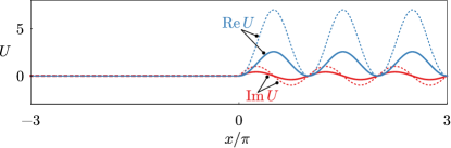
Figure 1: Real and imaginary parts of the potential $U(x)$ chosen for the numerical illustration. Solid and dotted lines correspond to $\gamma=0.4$ and $\gamma=1$, respectively. Real parts are shown up to irrelevant additive constant (which can be absorbed by a shift of the propagation constant).

For a numerical illustration, we focus on surface solitons at the interface of a complex periodic potential by choosing the Wadati potential given by (7) with $w_{1}(x)=\alpha/2$ and $w_{2}(x)=\alpha/2+\gamma\sin^{2}x$, where $\alpha$ is an auxiliary constant parameter that tunes the real background of the potential, and $\gamma>0$ is the amplitude of periodic modulation (see Fig. 1 for plots of the potential). The left semiaxis $x<0$ corresponds to a uniform conservative medium. The right halfspace $x>0$ is occupied by a complex-valued potential which (if considered on the entire real axis) is $\pi$-periodic and ${\cal PT}$ symmetric. The existence range of surface solitons is constrained by the combination of two different requirements. In the left semiaxis, the existence of a localized beam is possible only under the following requirement $\tilde{\beta}:=\beta-\alpha^{2}/4>0$. If the latter inequality holds, the asymptotic behavior of the decaying tail can be easily found as $\Psi_{-}(x;\beta)=e^{\sqrt{\tilde{\beta}}x}$. In the right semiaxis, a necessary requirement for the solution to be localized implies that $\tilde{\beta}$ belongs to a spectral gap of the complex periodic potential. By the Floquet theorem, in this case the asymptotic behavior is given as $\Psi_{+}(x;\beta)=e^{\lambda(\tilde{\beta})x}u(x;\tilde{\beta})$, where $\lambda(\tilde{\beta})$ is the characteristic exponent (Re $\lambda<0$), and $u(x;\tilde{\beta})$ is a $\pi$-periodic function of $x$. For each $\tilde{\beta}$ in the gap, $\lambda(\tilde{\beta})$ and corresponding function $u(x;\tilde{\beta})$ can be found numerically with the monodromy matrix approach. Using the established asymptotic behaviors, one can approximate the solutions for some $x=\pm L$, where $L\gg 1$ is a sufficiently large number, and use the Runge-Kutta method to compute $(\rho_{\pm}(0),\rho_{x,\pm}(0),v_{\pm}(0))$ for any $C_{+}$ and $C_{-}$.

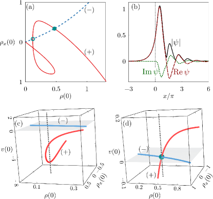
Figure 2: (a) Dependencies $(\rho_{\pm}(0),\rho_{\pm,x}(0),v_{\pm}(0))$ plotted as 2D curves (labelled with “$+$” and “$-$”, respectively) on the plane $(\rho(0),\rho_{x}(0))$. There are two intersections, one of which (marked with the open circle) corresponds to a spurious solution, and another one (marked with the filled circle) is a valid solution corresponding to a surface soliton. Panels (c,d) show the same dependencies in the 3D space (only the volumes close to the intersections are zoomed in): for the spurious solution there is no intersection in the 3D space (c), and for the valid solution there is a 3D intersection (d). Panel (b) illustrates the spatial profile of the surface soliton obtained from the valid intersection. Modulus of function $\psi$, its real and imaginary parts are labelled as $|\psi|$, $\mathrm{Re}\,\psi$, and $\mathrm{Im}\,\psi$, respectively. In this figure, $g=1$, $\alpha=6$, $\gamma=0.4$, $\tilde{\beta}=0.4$.

To illustrate the procedure of finding of surface solitons, in Fig. 2(a) we display a representative example of a diagram obtained with our numerical approach for a particular value of the propagation constant $\tilde{\beta}=0.4$ and for coefficients $C_{\pm}$ varying within the following intervals: $C_{+}\in[0,1.6]$, $C_{-}\in[0,0.8]$. The 2D diagram on the plane $(\rho(0),\rho_{x}(0))$ has two intersections, one of which corresponds to a spurious solution [no intersection in 3D diagram plotted in Fig. 2(c)], and another one is indeed a valid solution that corresponds to a surface soliton [there is a 3D intersection in Fig. 2(d)]. The surface soliton obtained from the valid intersection is shown in Fig. 2(b). It has complex internal structure with nontrivial real and imaginary parts. However, for $x\leq 0$, the imaginary part is identically zero, because the corresponding halfspace is conservative.

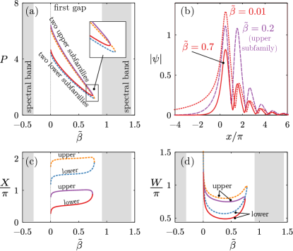
Figure 3: (a) Two families of surface solitons in the first finite gap plotted as the dependencies of the energy flow $P$ on the shifted propagation constant $\tilde{\beta}$. Each family consists of an upper and a lower subfamily which merge at a cutoff propagation constant (see the inset). Panels (c,d) display the same (sub)families plotted as dependencies of the center-of-mass $X$ and meanwidth $W$ on $\tilde{\beta}$. The correspondence between different subfamilies in (a,c,d) can be established using the labels “upper” and “lower”, solid and dashed lines, and colors (in the online version). Panel (b) shows moduli $|\psi|$ of two solitons from the lower subfamily closest to the interface at $\tilde{\beta}=0.7$ and $0.01$ and one soliton from the corresponding upper subfamily at $\tilde{\beta}=0.2$. In this figure, $g=1$, $\alpha=6$, $\gamma=0.4$.

Solution plotted in Fig. 2(b) belongs to a continuous family of surface solitons which can be obtained by varying the propagation constant and repeating the described procedure. Moreover, we have found that extending the range of parameters $C_{+}$ and $C_{-}$ it is possible to find multiple coexisting solutions and, respectively, multiple coexisting soliton families. Some of the found families, obtained in the defocusing medium for propagation constant lying in the first spectral gap, are presented in Fig. 3(a) as the dependencies of the energy flow $P=\int_{-\infty}^{\infty}|\psi|^{2}dx$ on the propagation constant. Each family consists of two subfamilies (“upper” and “lower”) with different values of $P$. The found families have different right cutoff values where the upper and lower subfamilies merge and disappear [see the inset in Fig. 3(a)]. Thus, similar to surface gap solitons in a conservative medium Karta2006 , our solutions exist only if the energy flow exceeds some nonzero threshold value. The found solitons can be also characterized using the center-of-mass $X=P^{-1}\int_{-\infty}^{\infty}x|\psi|^{2}dx$ and meanwidth $W=\sqrt{P^{-1}\int_{-\infty}^{\infty}(x-X)^{2}|\psi|^{2}dx}$, plotted in Fig. 3(c,d). Figure 3(c) indicates that there exists a sequence of families consisting of solitons whose centers are situated at different distances from the interface position $x=0$. In Fig. 3 we show only two families (resp., four subfamilies) that consist of solitons centered closest to the surface; there exist other families with larger positive values of center-of-mass $X$. Solitons from these large-$X$ families are effectively situated in the bulk periodic medium and hence become similar to the conventional gap solitons. For this reason they are not shown in Fig. 3.

Surface solitons from lower subfamilies are single-peaked, while solitons from the upper subfamilies contain two out-of-phase peaks with close amplitudes [see an example with $\tilde{\beta}=0.2$ in Fig. 3(b)]. As the propagation constant decreases, the surface solitons cease to exist in the limit $\tilde{\beta}\to+0$, where the left ‘halfsoliton’ loses the localization, while the right tail of the soliton remains well-localized [see an example with $\tilde{\beta}=0.01$ in Fig. 3(b)]. As a result, in the limit $\tilde{\beta}\to+0$ the solitons centers incline downwards in Fig. 3(c).

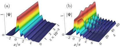
Figure 4: Propagation of stable (from the lower subfamily, panel a) and unstable (from the upper subfamily, panel b) surface solitons coexisting at $\tilde{\beta}=0.5$. Other parameters as in Fig. 3.

Linear stability analysis and dynamical simulations of soliton propagation indicate that solitons from upper subfamilies are strongly unstable, while those from lower subfamilies are stable. Examples of stable and unstable propagations are presented in Fig. 4. In this figure, each surface soliton has been initially perturbed by a $5\%$ complex-valued random noise and propagated according to Eq. (1).

Tuning the shape of the complex lattice in the right halfspace, it is possible to obtain a situation when the a priori left existence boundary $\tilde{\beta}=0$ belongs to the spectral band (and not to the gap as in Fig. 3). In this case, the decrease of the propagation constant continues the soliton families up to the band edge, where the right halfsoliton becomes delocalized, while the left tail remains localized, as illustrated in Fig. 5.

To conclude, we have demonstrated that non-Hermitian surface solitons form continuous families in complex potentials of a certain shape. This result has been illustrated for gap-surface solitons guided by an interface between a homogeneous medium and a ${\cal PT}$-symmetric potential. The surface solitons have complex-valued internal structure and feature different existence ranges and delocalization scenarious depending on the relationship between the edge of the continuous spectrum of the uniform medium and the band-gap structure of the periodic potential. Regarding the future research, our results can be immediately generalized to surface solitons at an interface of a non-${\cal PT}$-symmetric and/or nonperiodic potential. A generalization to a focusing medium is also straightforward. Wadati potentials can be conveniently used to study surface soliton families in lattices with modulated separation between the cells (similar to those in Karta2019 ). A generalization to two transverse directions is also possible. An important byproduct of our study is a previously unexplored class of layered Wadati potentials composed of several continuously concatenated functions. These potentials also admit soliton families and are worth further study.

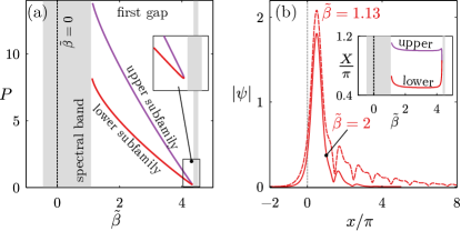
Figure 5: Families of surface solitons when the a priori left existence boundary $\tilde{\beta}=0$ lies inside a spectral band (a) and examples of soliton profiles from the lower subfamily (b). Inset in (b) shows the centers-of-mass [compare with Fig. 3(c)]. In this figure, $g=1$, $\alpha=6$, $\gamma=1$.

Funding. Ministry of Science and Higher Education of Russian Federation, goszadanie no. 2019-1246.

References

- (1) D. Mihalache, M. Bertolotti, and C. Sibilia, Prog. Opt. 27, 229–313 (1989).
- (2) A. D. Boardman, P. Egan, F. Lederer, U. Langbein, and D. Mihalache, in Nonlinear Surface Electromagnetic Phenomena, H. E. Ponath and G. I. Stegeman, eds. (North-Holland, 1991), p. 73.
- (3) N. N. Akhmediev and A. Ankiewicz, Solitons: Nonlinear Pulses and Beams (Chapman & Hall, 1997).
- (4) K. G. Makris, S. Suntsov, D. N. Christodoulides, and G. I. Stegeman, Opt. Lett. 30, 2466 (2005).
- (5) Y. V. Kartashov, V. A. Vysloukh, and Ll. Torner, Phys. Rev. Lett. 96, 073901 (2006).
- (6) F. Lederer, G. I. Stegeman, D. N. Christodoulides, G. Assanto, M. Segev, and Y. Silberberg, Phys. Rep. 463, 1–126 (2008).
- (7) Y. V. Kartashov, B. A. Malomed, and Ll. Torner, Rev. Mod. Phys. 83, 247 (2009).
- (8) N. Akhmediev and A. Ankiewicz, Three sources and three component parts of the concept of dissipative solitons. In: Akhmediev N, Ankiewicz A, eds. Dissipative Solitons: From Optics to Biology and Medicine. Springer-Verlag; 2008: 1–29.
- (9) N. N. Rozanov, J. Opt. Technol. 76, 187 (2009).
- (10) V. V. Konotop, J. Yang, and D. A. Zezyulin, Rev. Mod. Phys. 88, 035002 (2016).
- (11) L. Feng, R. El-Ganainy, and L. Ge, Nat. Photon. 11, 752–762 (2017).
- (12) D. Mihalache, D. Mazilu, F. Lederer, and Yu. S. Kivshar, Phys. Rev. A 77, 043828 (2008).
- (13) Y. V. Kartashov, V. V. Konotop, V. A. Vysloukh, EPL 91, 34003 (2010).
- (14) Y. He, D. Mihalache, X. Zhu, L. Guo, and Y. V. Kartashov, Opt. Lett. 37, 2526 (2012).
- (15) Huagang Li, Zhiwei Shi, Xiujuan Jiang, Xing Zhu, Tianshu Lai, and Chaohong Lee, Opt. Lett. 39, 5154–5157 (2014).
- (16) Y. V. Kartashov and D. V. Skryabin, Phys. Rev. Lett. 119, 253904 (2017).
- (17) Ting-Wei Che and Szu-Cheng Cheng, Phys. Rev. E 98, 032212 (2018).
- (18) D. A. Dobrykh, A. V. Yulin, A. P. Slobozhanyuk, A. N. Poddubny, and Yu. S. Kivshar, Phys. Rev. Lett. 121, 163901 (2018).
- (19) C. Huang and L. Dong, Opt. Lett. 44, 5438–5441 (2019).
- (20) Y. V. Kartashov and V. A. Vysloukh, Opt. Lett. 44, 791 (2019).
- (21) Y. V. Kartashov, V. A. Vysloukh, Opt. Lett. 44, 5469 (2019).
- (22) M. Wadati, J. Phys. Soc. Jpn. 77, 074005 (2008).
- (23) A. C. Newell, Solitons in Mathematics and Physics (SIAM, 1985).
- (24) G. L. Lamb, Jr., Elements of Soliton Theory (Wiley, 1980).
- (25) C. Hang, G. Gabadadze, and G. Huang, Phys. Rev. A 95, 023833 (2017).
- (26) E. N. Tsoy, I. M. Allayarov, and F. Kh. Abdullaev, Opt. Lett. 39, 4215 (2014).
- (27) V. V. Konotop and D. A. Zezyulin, Opt. Lett. 39, 5535 (2014).
- (28) J. Yang, Stud. Appl. Math. 147, 4 (2021).