Realtime dynamics of hyperon spin correlations
from string fragmentation in a deformed four-flavor Schwinger model

Abstract

Self-polarizing weak decays of $\Lambda$-hyperons provide unique insight into the role of entanglement in the fragmentation of QCD strings through measurements of the spin correlations of $\Lambda{\bar{\Lambda}}$-pairs produced in collider experiments. The simplest quantum field theory representing the underlying parton dynamics is the four-flavor massive Schwinger model plus an effective spin-flip term, where the flavors are mapped to light (up/down) and heavy (strange) quarks and their spins. This construction provides a novel way to explore hyperon spin-correlations in 1+1-dimensions. We investigate the evolution of these correlations for different string configurations that are sensitive to the rich structure of the model Hamiltonian.

An intriguing question in QCD and QCD-like theories is the role of entanglement in the confinement of quarks and gluons (partons) within hadrons Klebanov et al. (2008); Beane et al. (2019). In high energy QCD, features of entanglement were explored recently in the context of parton distributions in deeply inelastic scattering Kharzeev and Levin (2017); Armesto et al. (2019); Hentschinski and Kutak (2022); Dumitru and Kolbusz (2022); Dumitru et al. (2023); Hentschinski et al. (2023); Asadi and Vaidya (2023); Duan et al. (2023); Ramos and Machado (2020); Beane and Ehlers (2019) and in parton fragmentation into hadrons Berges et al. (2018a, b); Neill and Waalewijn (2019); Gong et al. (2022); Benito-Calviño et al. (2023); Barata et al. (2023a, b). A strong motivation is the promise of fresh insight from quantum information science (QIS) into these fundamental quantum many-body parton features of hadrons  Dvali and Venugopalan (2022); Dvali (2021); Kharzeev (2021); Kou et al. (2022); Klco and Savage (2021).

Several proposals have emerged for quantum entanglement and Bell-type inequality measures in the challenging environment of collider experiments Hao et al. (2010); Barr (2022); Fabbrichesi et al. (2021); Afik and de Nova (2023); Klco and Beck (2023); Ashby-Pickering et al. (2023); Florio et al. (2023). In Gong et al. (2022), two of us proposed that the self-polarizing weak decays of hyperons can be exploited to measure $\Lambda{\bar{\Lambda}}$ spin correlations in the fragmentation of QCD strings. Following earlier work Tornqvist (1981) on the Clauser-Horne-Shimony-Holt (CHSH) Clauser et al. (1969) for $\Lambda{\bar{\Lambda}}$ spin correlations, we constructed a modified CHSH inequality and entanglement measures of the string spin density matrix. Since $\Lambda$ (${\bar{\Lambda}}$) hyperons contain a flavor triplet of up, down and strange (anti)quarks, measurements of their spin correlations probe quantum features of parton dynamics within QCD strings. In particular, clean extraction of hyperon spin correlations Tu (2023) will be possible at the future Electron Ion Collider Accardi et al. (2016).

Further progress exploiting the potential of hyperon spin correlations requires a dynamical model of parton dynamics in the formation and fragmentation of QCD strings. Nonperturbative first principles quantum field theory (QFT) methods such as lattice QCD are inapplicable because of the intrinsically realtime dynamics of hadronization. Therefore phenomenological models are the state-of-the art in describing hadronization at colliders, the quintessential example being the Lund string model Andersson et al. (1983) implemented in the widely used event generator PYTHIA Sjöstrand et al. (2015). Since these models are semi-classical in nature, computations on quantum devices offer a promising path towards performing first principles simulations of string dynamics Bañuls et al. (2020); Di Meglio et al. (2023); Bauer et al. (2023). Due to the complexity of this program, efforts in this direction have focused on 1+1-d QFT’s. While the extension to QCD is challenging, such studies can help towards implementing QIS features in phenomenological frameworks in the near future Hunt-Smith and Skands (2020).

In this letter, we will outline the simplest 1+1-dimensional QFT that captures the rich flavor and spin dynamics of light and heavy partons in the QCD string, allowing us to model quantum features of $\Lambda{\bar{\Lambda}}$-correlations for the first time. Our work significantly extends the static string configuration study in Gong et al. (2022); these efforts are timely, motivating experimental measurements of hyperon spin correlations at colliders Vanek (2023). We will assume, as in the nonrelativistic quark model, that $\Lambda$-spin is carried by the heavy strange quark. The status of this ansatz is uncertain; for proposed experimental tests, see Burkardt and Jaffe (1993); Moretti (2018); Ellis and Hwang (2012); Metz and Vossen (2016); Tu (2023).

To construct our QFT model of parton dynamics in the QCD string, we start from the massive Schwinger model (1+1-d QED) with $N_{f}=4$ quark flavors . In temporal gauge $A_{0}=0$, this model is described by the Hamiltonian

$$H_{\rm Schwinger}=\int dx\,\frac{1}{2}E^{2}(x)$$

$$+ \sum_{f=1}^{N_{f}=4}\bar{\psi}_{f}(x)(-i\gamma^{1}\partial_{1}+g\gamma^{1}A_{1}(x)+m_{f})\psi_{f}(x)\,,$$ (1)

where $g$ is the dimensionful coupling constant and the electric field $E=-F^{01}=-\partial^{0}A^{1}$, with $A_{1}$ denoting the other component of the $U(1)$ gauge field. Note that there is no magnetic field in 1+1-dimensions. The two component fermion spinors $\psi_{f}$, with flavor indices $f=1,2,3,4$, satisfy the canonical commutation relations,

$$\{\psi_{f}(x),\psi_{l}(y)\}=0\,\,;\,\,\{\psi^{\dagger}_{f}(x),\psi_{l}(y)\}=\delta(x-y)\,\delta_{f,l}\,.$$ (2)

The electric field satisfies Gauss’ law, $\partial_{x}E=g\sum_{f}\psi_{f}^{\dagger}\psi_{f}$; it is not a dynamical degree of freedom and can be explicitly integrated out.

To adapt this model to our problem of hyperon spin correlations, we first make the simplifying assumption that since the ratio of the physical up and down quark masses is $m_{u}/m_{d}\sim\mathcal{O}(1)$ Workman et al. (2022), their dynamics are indistinguishable. Further, since the mass gap between the heavy strange flavor and these light flavors is $m_{s}/(m_{d}+m_{u})\sim\mathcal{O}(10)$, it is sufficient to simply consider a light and a heavy flavor fermion in our study. Because the structure of the Lorentz group dictates that there is no notion of spin in 1+1-dimensions, we will construct an effective model of spin dynamics using the map [flavor ($f$) $\to$ (species ($s$), spin ($\sigma$))]:

$$1\to(h,{\uparrow})\,\,;\,\,2\to(h,{\downarrow})\,\,;\,\,3\to(l,{\uparrow})\,\,;\,\,4\to(l,{\downarrow})\,,$$ (3)

where the $h,l$ indices denote the heavy and light fermions, with masses $m_{h}$ and $m_{l}\ll m_{h}$, while ${\uparrow},{\downarrow}$ correspond to their up or down spin state. Using this double label $(s,\sigma)$, we have therefore mapped the four two-component spinors to two four-component spinors, and Eq. (2) satisfies the 3+1-d QED anticommutation relations with $\delta_{l,f}\to\delta_{s,s^{\prime}}\delta_{\sigma,\sigma^{\prime}}$. Due to the large mass gap between fermionic species, the global flavor symmetry group of Eq. (Realtime dynamics of hyperon spin correlations from string fragmentation in a deformed four-flavor Schwinger model) reduces from ${\rm SU}_{f}(4)\to{\rm SU}_{h}(2)\times{\rm SU}_{l}(2)$.

An important difference from 3+1-d QED is the absence of magnetic fields in 1+1-d; there are therefore no Thomas precession or Larmor interaction terms. However we anticipate that such interactions would be suppressed for our problem of interest . The spin-dependent interactions of light and heavy flavors in the QCD string are therefore well-approximated by adding to Eq. (Realtime dynamics of hyperon spin correlations from string fragmentation in a deformed four-flavor Schwinger model) the effective spin Hamiltonian

$$H_{\rm spin} =\int dx\,g_{ll}^{0}\,\bar{\psi}_{l,{\uparrow}}\gamma^{0}\psi_{l,{\downarrow}}+g_{ll}^{1}\,\bar{\psi}_{l,{\uparrow}}\psi_{l,{\downarrow}}$$

$$+g_{lh}^{0}(\bar{\psi}_{h,{\uparrow}}\gamma^{0}\psi_{l,{\downarrow}}+\bar{\psi}_{h,{\downarrow}}\gamma^{0}\psi_{l,{\uparrow}})$$

$$+g_{lh}^{1}(\bar{\psi}_{h,{\uparrow}}\psi_{l,{\downarrow}}+\bar{\psi}_{h,{\downarrow}}\psi_{l,{\uparrow}})+{\rm h.c.}\,,$$ (4)

where we used the mapping in Eq. (3). The first two terms describe the spin-flip interactions between the light fermions with their respective coupling constants. The subsequent terms describe the spin interactions between light and heavy fermions. Direct heavy spin-flip interactions are assumed to be suppressed by their large mass . The addition of $H_{\rm spin}$ reduces the global symmetry of the $N_{f}=4$ Schwinger model from ${\rm SU}_{h}(2)\times{\rm SU}_{l}(2)\to{\rm SU}_{\rm spin}(2)$ corresponding to the symmetry group of light and heavy quarks in the QCD string .

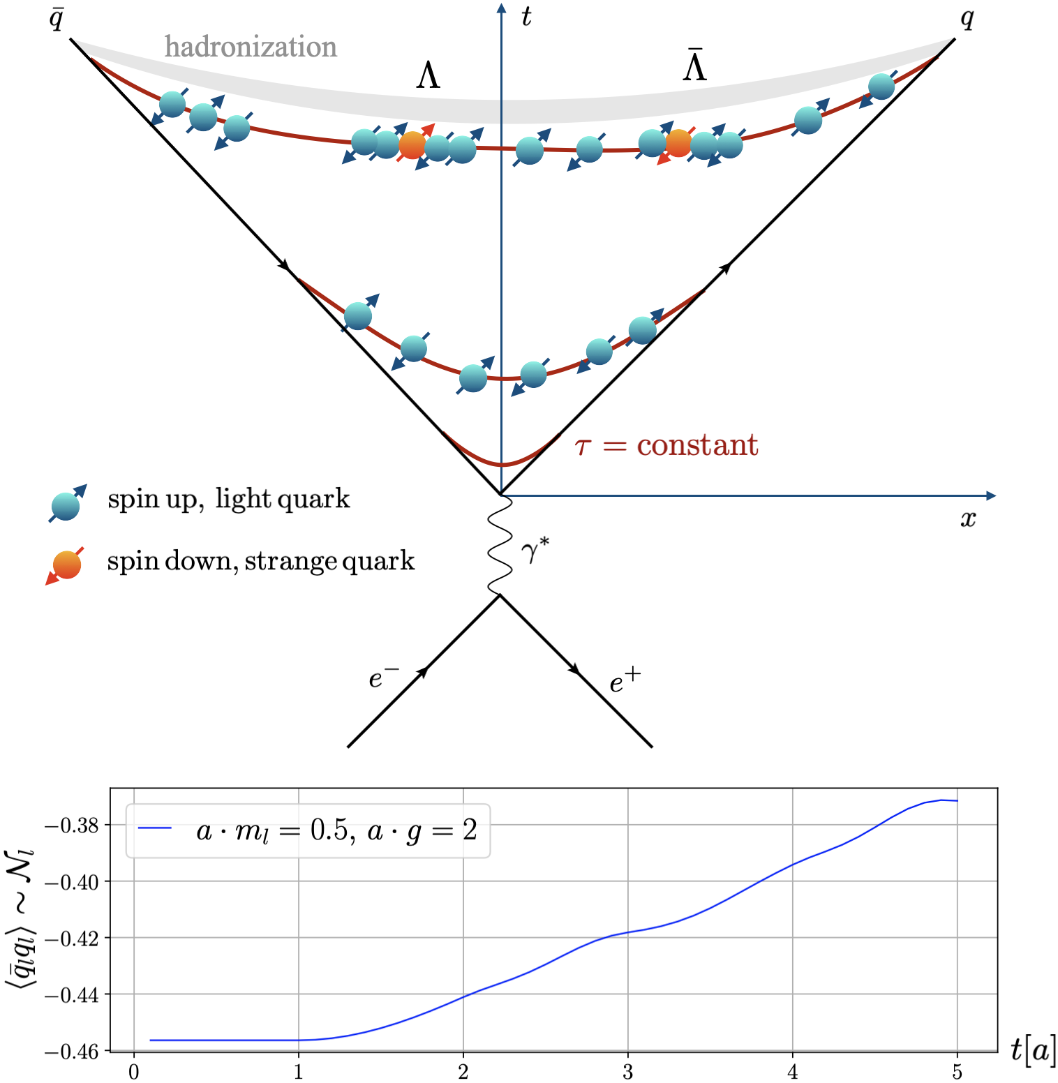
Figure 1: Top: Illustration of realtime evolution of the confining string described by the model Hamiltonian $H=H_{\rm Schwinger}+H_{\rm Spin}$. The string stretched between a $q\bar{q}$ pair moving along the forward light-cone is increasingly populated by light quarks with each proper time $\tau$ slice. The heavy quark multiplicity is suppressed due to its larger mass and its spin is modified primarily due to multiparticle interactions. Bottom: Lattice computation in the $N_{f}=1$ massive Schwinger model for the light quark correlator $\langle\bar{q}_{l}q_{l}\rangle$ correlator. For $m_{l}<g$, the increase of this observable is directly related to a larger multiplicity of light quarks $\mathcal{N}_{l}$ within the string as shown in the illustration. Details of figures in main text.

The model deformed Hamiltonian $H=H_{\rm Schwinger}+H_{\rm spin}$ can be employed to explore the realtime dynamics of spin correlations between heavy fermions in the dynamical process $e^{+}e^{-}\rightarrow{q{\bar{q}}}\rightarrow\Lambda{\bar{\Lambda}}+X$ illustrated in Fig. 1 (top). Recall that we treat strange quark (antiquark) spin as a proxy for $\Lambda$ (${\bar{\Lambda}}$) spin in our model. The qualitative picture of this process is as follows. The injection of energy from the virtual photon forms the primordial $q{\bar{q}}$ pair. Additional pair production taking place due to the Schwinger mechanism Grib et al. (1994); Schwinger (1951) is demonstrated by explicit computation using tensor network techniques (discussed below) for the $N_{f}=1$ case in Fig. 1 (bottom) for an expanding QCD string. As shown in Fig. 1 (top), the string should be mostly populated by light quarks. The light and strange quarks carry spin and their self-interactions generate nontrivial correlations between the rarer heavy strange quark pairs, with the multiparton quantum dynamics reflected in the $\Lambda\bar{\Lambda}$ spin correlations measured in hyperon weak decays.

This complex dynamical evolution can be captured by extending the gauge sector in Eq. (Realtime dynamics of hyperon spin correlations from string fragmentation in a deformed four-flavor Schwinger model) to Casher et al. (1974); Honda et al. (2022); Nagano et al. (2023)

$$\int dx\,E^{2}(x)\to\int dx\,(E(x)+E_{\rm ext.}(x))^{2}\,.$$ (5)

The external field $E_{\rm ext.}$ plays the role of the embedding string, see Fig. 1 (top), taking the form

$$E_{\rm ext.}=-|Q|\,\Theta(x^{<}(t)<x<x^{>}(t))\,,$$ (6)

with $|Q|$ the absolute value of the external charges (the $q\bar{q}$ pair in Fig. 1 (top)) generating the field and $x^{>(<)}=+(-)t$ referring to their right (left) dynamical spatial positions along the forward lightcone. For analogous detailed studies of realtime evolution of pair production, charge separation and screening for the $N_{f}=1$ Schwinger model, see  Hebenstreit et al. (2013a, b); Hebenstreit and Berges (2014); Lee et al. (2023); Florio et al. (2023).

We will now explore in our $N_{f}=4$ framework the quantitative realization of the picture we have outlined. We discretize $H$ employing staggered fermions Susskind (1977); Banks et al. (1976) on a lattice with $N=40$ sites and lattice spacing $a$. The staggered discretization of the dimensionful continuous two component spinor $\psi_{f}$ leads to the dimensionless single component spinor $\chi_{s,\sigma}(\tilde{n})$ on the lattice – see the supplemental material for details. The lattice index $\tilde{n}=1,2,\cdots\tilde{N}=10$ labels the staggered sites; for each one of these, there are four computational lattice sites, labeled by $n=1,2,\cdots,40$, that follow the ordering implicit in Eq. 3 , as seen in Fig. 2. The single component spinor $\chi_{s,\sigma}(\tilde{n})$ represents fermions on even sites and antifermions on odd sites and it satisfies the commutation relations

$$\{\chi_{s,\sigma}(\tilde{n}),\chi_{s^{\prime},\sigma^{\prime}}(\tilde{m})\}=0\,,$$

$$\{\chi_{s,\sigma}^{\dagger}(\tilde{n}),\chi_{s^{\prime},\sigma^{\prime}}(\tilde{m})\}=\delta_{\tilde{n},\tilde{m}}\delta_{s,s^{\prime}}\delta_{\sigma,\sigma^{\prime}}\,.$$ (7)

Since Gauss’ law, as noted previously, dictates that the electric field is not dynamical, all dependence on gauge fields can be integrated out, resulting in a (nonlocal) expression for $H_{\rm Schwinger}$ entirely in terms of $\chi$. This is also the case for $H_{\rm spin}$. The corresponding lattice expressions are provided in the supplemental material.

With the goal of simulating the model using tensor network methods, we further map the lattice Hamiltonian to a one-dimensional spin chain model via a multiflavor Jordan Wigner transform (JWt) Steinhardt (1977); Banks et al. (1976); Steinhardt (1977); Bañuls et al. (2017) which, for our particular case, can be expressed as

$$\chi_{h,\uparrow}(\tilde{n})=S(\tilde{n})\sigma^{-}_{h,\uparrow}(\tilde{n})\,;$$

$$\chi_{h,\downarrow}(\tilde{n})=iS(\tilde{n})\sigma^{z}_{h,\uparrow}(\tilde{n})\sigma^{-}_{h,\downarrow}(\tilde{n})\,;$$

$$\chi_{l,\uparrow}(\tilde{n})=-S(\tilde{n})\sigma^{z}_{h,\uparrow}(\tilde{n})\sigma^{z}_{h,\downarrow}(\tilde{n})\sigma^{-}_{l,\uparrow}(\tilde{n})\,;$$

$$\chi_{l,\downarrow}(\tilde{n})=-iS(\tilde{n})\sigma^{z}_{h,\uparrow}(\tilde{n})\sigma^{z}_{h,\downarrow}(\tilde{n})\sigma^{z}_{l,\uparrow}(\tilde{n})\sigma^{-}_{l,\downarrow}(\tilde{n})\,;$$ (8)

where we introduced the string operator

$$S(\tilde{n})\equiv\prod_{\tilde{k}<\tilde{n}}[\sigma^{z}_{h,\uparrow}(\tilde{k})\sigma^{z}_{h,\downarrow}(\tilde{k})\sigma^{z}_{l,\uparrow}(\tilde{k})\sigma^{z}_{l,\downarrow}(\tilde{k})]\,,$$ (9)

in terms of local Pauli operators $\sigma^{i}_{s,\sigma}(\tilde{n})$ acting on site $\tilde{n}$ of the staggered lattice. The subscript indicates the flavor and spin indices and the superscript denotes the direction in the Bloch sphere. With these identifications, our model Hamiltonian can be mapped to a spin chain with the Hamiltonian

$$H_{\rm lat} =\frac{1}{2}g^{2}a\sum_{\tilde{n}=1}^{\tilde{N}-1}\Big{[}\frac{1}{2}\sum_{s,\sigma}\sum_{\tilde{k}=1}^{\tilde{n}}(\sigma^{z}_{s,\sigma}(\tilde{k})+(-1)^{\tilde{k}})\Big{]}^{2}+\sum_{\tilde{n}=1}^{\tilde{N}}\sum_{s,\sigma}m_{s}(-1)^{\tilde{n}}\left(\frac{1+\sigma^{z}_{s,\sigma}(\tilde{n})}{2}\right)$$

$$+\frac{i}{2a}\sum_{n=1}^{N_{f}(\tilde{N}-1)}(\sigma^{+}(n)\sigma^{z}(n+1)\sigma^{z}(n+2)\sigma^{z}(n+3)\sigma^{-}(n+4)-\sigma^{+}(n+4)\sigma^{z}(n+3)\sigma^{z}(n+2)\sigma^{z}(n+1)\sigma^{-}(n))$$

$$+\sum_{\tilde{n}=1}^{\tilde{N}}(-i)(g_{ll}^{0}+g_{ll}^{1}(-1)^{\tilde{n}})(\sigma^{+}_{l,{\uparrow}}(\tilde{n})\sigma^{-}_{l,{\downarrow}}(\tilde{n})-\sigma^{+}_{l,{\downarrow}}(\tilde{n})\sigma^{-}_{l,{\uparrow}}(\tilde{n}))+i(g_{lh}^{0}+g_{lh}^{1}(-1)^{\tilde{n}})(\sigma^{+}_{h,{\uparrow}}(\tilde{n})\sigma^{z}_{h,{\downarrow}}(\tilde{n})\sigma^{z}_{l,{\uparrow}}(\tilde{n})\sigma^{-}_{l,{\downarrow}}(\tilde{n})$$

$$-\sigma^{+}_{l,{\downarrow}}(\tilde{n})\sigma^{z}_{l,{\uparrow}}(\tilde{n})\sigma^{z}_{h,{\downarrow}}(\tilde{n})\sigma^{-}_{h,{\uparrow}}(\tilde{n})+\sigma_{l,{\uparrow}}^{+}(\tilde{n})\sigma^{-}_{h,{\downarrow}}(\tilde{n})-\sigma_{h,{\downarrow}}^{+}(\tilde{n})\sigma^{-}_{l,{\uparrow}}(\tilde{n}))\,,$$ (10)

where $s={l,h}$, $\sigma={{\uparrow},{\downarrow}}$ and the second line is indexed with respect to the computational lattice. We can now employ tensor network methods to study the heavy flavor spin dynamics of $H_{\rm lat}$.

Due to the complexity of the process outlined in Fig. 1, and the well-known limitations of tensor networks in performing realtime evolution, we restrict ourselves to a simpler yet highly illustrative setup. Using our 40 site lattice, we first prepare the ground state of the system for $g_{ll}^{0}=g_{ll}^{1}=g_{lh}^{0}=g_{lh}^{0}=0$; this corresponds to the ground state of the four-flavor massive Schwinger model at finite coupling . We adopt a matrix product state (MPS) architecture using the density matrix renormalization group (DMRG) algorithm White (1992, 1993). We then time evolve the system under the full Hamiltonian with finite spin couplings, inserting a static external electric in the middle of the lattice (between lattice sites 9 and 32) as shown in Fig. 2. The evolution time is chosen to be $t=a$  and is performed using the time-dependent variational principle (TDVP) algorithm Haegeman et al. (2011, 2016). Observables are computed on the time evolved state in the region spanned by the external field; note that its spatial extent is chosen to minimize boundary effects due to open boundary conditions and to maximize the number of usable lattice points. All simulations are performed using the tensor network package ITensor Fishman et al. (2022) in Julia for the parameter set $a\cdot g=2$, $a\cdot m_{l}=0.5$ and $a\cdot m_{h}=7.5$. The bare fermions masses are chosen such that their ratio is of the order of $m_{s}/(m_{u}+m_{d})$ and they include the improvement term  discussed in Dempsey et al. (2022, 2023).

To illustrate the key features of our model, we begin by computing the one point fermion correlator $\langle\bar{\psi}\psi\rangle_{n}$; the subscript denotes the expectation value at site $n$. As illustrated in Fig. 2, the ground state is characterized by two condensates (in blue), for each of the two fermion species. The light fermions have a larger value for the condensate. After time evolution (in red), light fermion pairs are easily excited in the region where the electric field is activated (denoted by the gold $q$/$\bar{q}$ labels), and the heavy and light condensates disappear. For both species, the points are grouped in doublets; this reflects the residual ${\rm SU}_{\rm spin}(2)$ symmetry of the model.

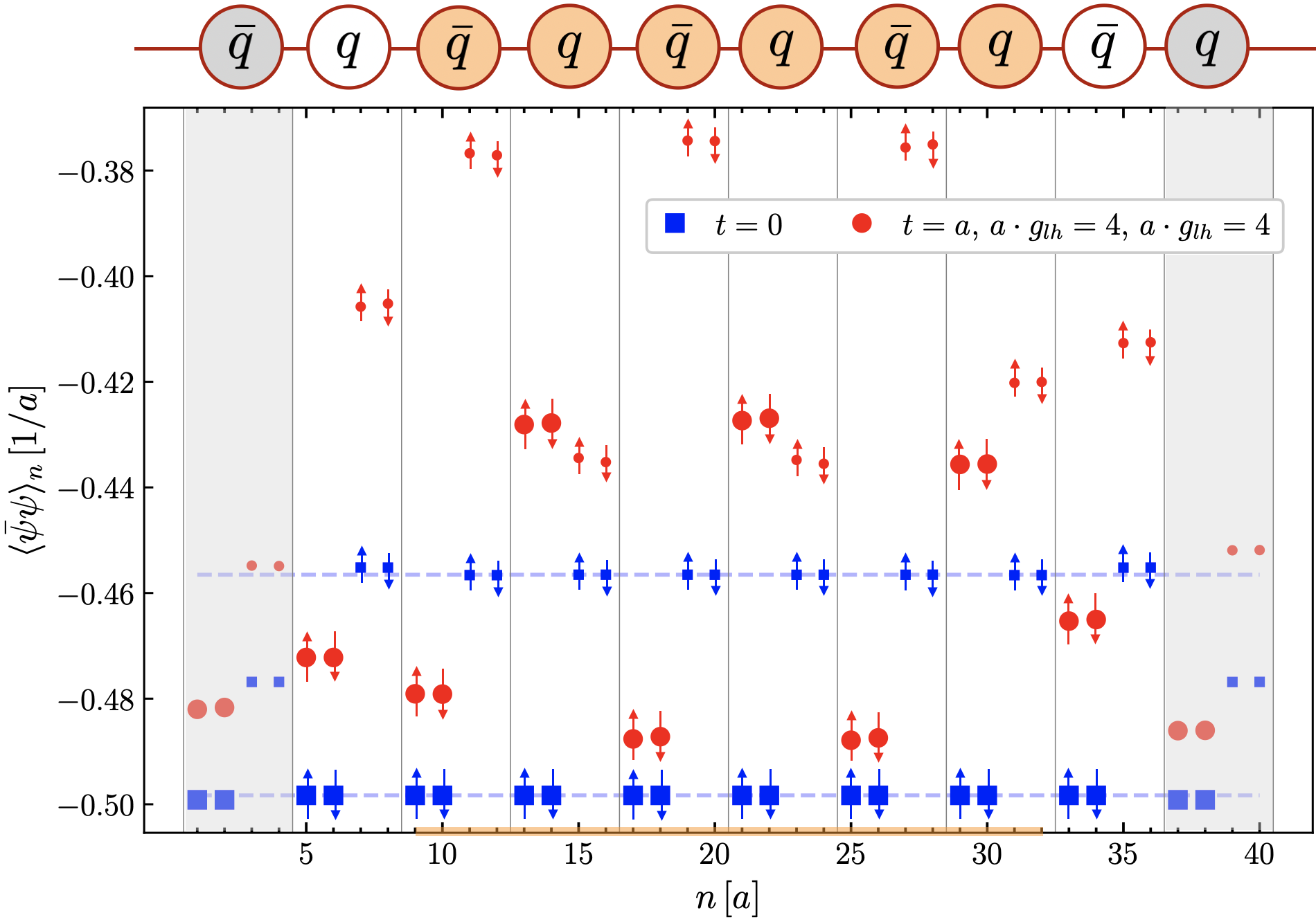
Figure 2: Lattice distribution of local one point function $\langle\bar{\psi}\psi\rangle_{n}$. At top is depicted the staggered construction alternating between fermions ($q$) and antifermions ($\bar{q}$). Each staggered site corresponds to four computational sites. Gray bands mark where lattice artifacts prevail. Gold band at the bottom (and gold $q$/$\bar{q}$ symbols) indicates where the external electric is active. Thick [thin] blue and red symbols represent heavy [light] fermion sites for ground ($t=0$) and excited ($t=a$) states respectively. Particle spins are denoted by $\uparrow\downarrow$. Dashed lines denote the ground state condensate for each particle species.

To study spin correlations of the heavy (strange) quarks, we introduce the fermion correlator

$$C_{\sigma,\sigma^{\prime}}(\Delta)\equiv\frac{\sum\limits_{\tilde{n},\tilde{m}}\langle\hat{c}_{\sigma}(\tilde{n})\hat{c}_{\sigma^{\prime}}(\tilde{m})\rangle_{\rm conn.}\,\delta_{\Delta,\tilde{n}-\tilde{m}}}{\sum\limits_{\tilde{n},\tilde{m}}\delta_{\Delta,\tilde{n}-\tilde{m}}}\,,$$ (11)

where $\Delta=1,2,3,\cdots$ is the spatial lattice separation, $\tilde{n}$, $\tilde{m}$ are chosen such that they correlate fermions with antifermions, with the operator

$$\hat{c}_{\sigma}(\tilde{n})=\bar{\psi}_{h,\sigma}\psi_{h,\sigma}-\langle\bar{\psi}_{h,\sigma}\psi_{h,\sigma}\rangle_{\rm\ket{\psi}_{t=0}}\,,$$ (12)

evaluated at the staggered site $\tilde{n}$. We subtract the ground state expectation value to minimize the dependence on the initial state; the connected correlator eliminates classical correlations.

In Fig. 3 we show numerical results for the $C_{{\uparrow},{\downarrow}}$ correlator. For the initial state (gray band), the correlator takes small values and vanishes for large lattice separations. The same occurs for $g_{lh}=0$ (red and pink curves) corresponding to no spin-flips between the two fermions species, or when $g_{ll}=0$ and at (small) finite $g_{lh}$ (black and gold circles). In the absence of direct spin interactions between the different species, there is no efficient mechanism to generate nontrivial correlations: the result is expected when $g_{ll}$ is nonzero; the fact it also holds when only the $g_{lh}$ coupling is activated indicates the system prefers to generate correlations between heavy fermions indirectly through spin exchanges via the light degrees of freedom. This is consistent what one would anticipate in QCD (see Fig. 1), where strange quark spin correlations are highly sensitive to the lighter degrees of freedom present in the string. Our conclusion is further supported by the other curves in Fig. 3. As $g_{lh}$ increases, generating stronger interactions between light and heavy fermions, short and long range correlations build up. Calculations performed for $C_{{\uparrow},{\downarrow}}$ exhibit quantitatively similar results. This is to be expected since our initial state is not prepared in a particular heavy fermion spin state.

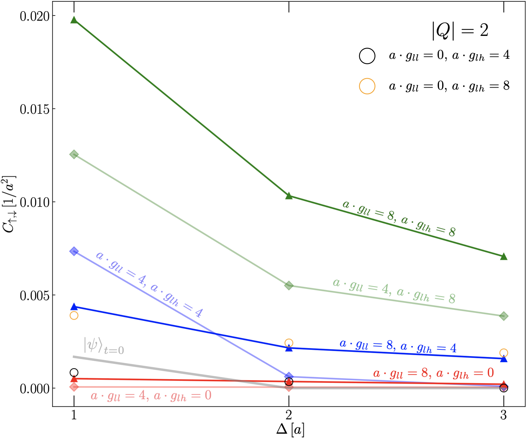
Figure 3: Heavy fermion correlator $C_{{\uparrow},{\downarrow}}$ as a function of the lattice separation $\Delta$. The electric field is generated with $|Q|=2$. The different colors depict the parameter sets used; the curve corresponding to the initial state is shown in gray.

Finally in Fig. 4, we plot the half-chain entanglement entropy, which can be easily extracted from the MPS. Since the initial state is not empty, we subtract the entropy present in the initial state: $\Delta S=S-S_{\ket{\psi}_{t=0}}$. As expected, larger values of the electric field result in a larger entanglement entropy, while $\Delta S$ also increases as a functions of $g_{lh}$. These results are in agreement with the behavior seen in Fig. 3, with larger correlations being reflected in larger $\Delta S$. However numerical simulations with other parameter sets show that the evolution of the entropy as a function of $g_{lh}$ can be nonmonotonic. This is not surprising since the connection between $\Delta S$ and correlation functions of the form of $C_{\sigma,\sigma^{\prime}}$ is in general nontrivial Gong et al. (2022); we leave a more in-depth study of the time dependence of $\Delta S$ to future work.

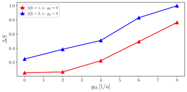
Figure 4: Half-chain entropy as a function of the $g_{lh}$ coupling.

In summary, ongoing studies of $\Lambda$ hyperon spin correlations at colliders offer unique insight into quantum features of fragmentation and hadronization in QCD strings. To model the underlying dynamics, we constructed and explored the simplest QFT that captures fundamental aspects of the formation and many-body dynamics of heavy and light flavors in a QCD string. Though relatively simple compared to QCD, this spin model has an extremely rich phase structure worthy of study in its own right.

Further progress is at present hindered on several fronts that deserve further attention. While our tensor network study can potentially be extended to larger lattices by further numerical optimization, time evolution still poses a challenge. Exact diagonalization can circumvent the latter; its application is however restricted to small lattices. Quantum computers have the potential to overcome both these constraints thereby demonstrating quantitative progress in a problem of fundamental interest in collider physics. We hope our manuscript spurs further developments in this direction.

Acknowledgments
J.B and R.V are supported by the U.S. Department of Energy under contract DE-SC0012704. This material is based upon work supported by the U.S. Department of Energy, Office of Science, National Quantum Information Science Research Centers, Co-design Center for Quantum Advantage (C2QA) under contract number DE-SC0012704. W.G is supported by the Center for Theoretical Physics at the Massachusetts Institute of Technology, the Paul and Daisy Soros Fellowship for New Americans, and the Hertz Foundation Fellowship. W.G would also like to thank the BNL Nuclear Theory Group and C2QA for their hospitality and support during the completion of this work. R.V.’s work on this topic was supported in part by the Simons Foundation under Award number 994318. He would like to thank Ross Dempsey and Igor Klebanov for valuable discussions. We are also grateful to Adrien Florio and Andreas Weichselbaum for clarifications of their work.

Supplemental Material

To obtain the lattice version of $H$, we discretize the fermionic and gauge degrees of freedom in an one-dimensional lattice indexed by $n$. For the gauge field, we introduce the reduced electric field operator $L\equiv E/g$ and link variables Hamer et al. (1997); Rothe (2012)

$$U(n)=e^{i\theta(n)}=e^{-iagA_{1}(n)}\,,$$ (13)

where we use a compact form of the gauge field such that $0<\theta(n)<2\pi$. Notice that while $\theta(n)$ is defined at the lattice site $n$, the link variable $U(n)$ and the reduced electric field $L(n)$ are formally defined in between sites $n$ and $n+1$. One can then show that the gauge field and the reduced electric field form an action-angle set of coordinates, such that Banks et al. (1976)

$$[\theta(n),L(m)]=i\delta_{m,n}\,.$$ (14)

As a consequence, the Hilbert space of each spatial link can be given in terms of the eigenstates of $L$, i.e. $L\ket{l}=l\ket{l}$ where $l=0,\pm 1,\pm 2,\cdots$. The link operator $U(n)$ is responsible for raising or lowering the value of the local electric field, $e^{i\theta}\ket{l}=U\ket{l}=\ket{l+1}$. In this formulation, and working in the charge zero sector, physical states satisfy the local constraint

$$G(n)\ket{\psi}=0\,,$$ (15)

for all $n$. This relation is given in terms of the local generators of gauge transformations which read Bañuls et al. (2017)

$$G(n) =L(n)-L(n-1)-\sum_{f}\Bigg{(}\chi_{f}^{\dagger}(n)\chi_{f}(n)$$

$$-\frac{1}{2}(1-(-1)^{n})\Bigg{)}\,.$$ (16)

We can use this relation to directly integrate out the gauge field on the lattice, when using open boundary conditions such that $L(0)=0$. Then, for each $n$, one can obtain the electric field on the $n$th link by iteration of the relation

$$L(n) =L(n-1)$$

$$+\sum_{f}\Bigg{(}\chi_{f}^{\dagger}(n)\chi_{f}(n)-\frac{1}{2}(1-(-1)^{n})\Bigg{)}\,.$$ (17)

The fermionic field is discretized using the staggered formulation Susskind (1977); Banks et al. (1976). This is generally described by the map between the continuum spinor field $\psi_{f}(x=na)$ and the lattice spinor $\chi_{f}(n)$

$$\psi_{f}(na)\to\frac{1}{\sqrt{a}}\begin{pmatrix}\chi_{f}(2n)\\ \chi_{f}(2n+1)\end{pmatrix}\,.$$ (18)

As explained in the main text, the flavor degeneracy for each lattice is lifted by creating $N_{f}$ copies of the same staggered site. Using Eq. (18), we can write the lattice versions of different elements of $H$; for the fermionic sector we have Susskind (1977):

$$\int dx\,m_{f}\bar{\psi}_{f}(x)\psi_{f}(x)\to\sum_{n=1}^{N}m_{f}(-1)^{n}\chi^{\dagger}_{f}(n)\chi_{f}(n)\,,$$ (19)

$$H_{\rm spin}\to\sum_{n=1}^{N}(g_{ll}^{0}+g_{ll}^{1}(-1)^{n})(\chi^{\dagger}_{l,{\uparrow}}(n)\chi_{l,{\downarrow}}(n))$$

$$+(g_{lh}^{0}+g_{lh}^{1}(-1)^{n})(\chi^{\dagger}_{h,{\uparrow}}(n)\chi_{l,{\downarrow}}(n)+\chi^{\dagger}_{h,{\downarrow}}(n)\chi_{l,{\uparrow}}(n))$$

$$+{\rm h.c.}\,,$$ (20)

$$\int dx\,\bar{\psi}_{f}(x) (-i\gamma^{1}\partial_{1}+g\gamma^{1}A_{1}(x))\psi_{f}(x)$$

$$\to-\frac{i}{2a}\sum_{n=1}^{N-1}\chi_{f}^{\dagger}(n)U(n)\chi_{f}(n+1)-{\rm h.c.}\,.$$ (21)

Here $U(n)$ ensures that the operator is invariant under gauge transformations and expanding $U(n)$ to leading order in $a$, it is straightforward to see that the covariant derivative structure is recovered in the continuum limit. Since we wish to work in a purely fermionic form of the theory, we perform a residual gauge transformation $\chi_{f}(n)\to\prod_{k<n}U(-k)\chi_{f}(n)$ Hamer et al. (1997), such that using open boundary conditions the gauge connection disappears from Eq. (Supplemental Material).

Finally, the purely gauge component can be written as

$$\frac{1}{2}\int dx\,E^{2}(x)\to\frac{1}{2}g^{2}a\sum_{n=1}^{N-1}L^{2}(n)\,.$$ (22)

Imposing Gauss’ law we can rewrite the gauge sector in terms of a long range potential term for the matter content, reading

$$\frac{1}{2}g^{2}a\sum_{n=1}^{N-1}\Big{[}\sum_{f}\sum_{k=1}^{n}\chi^{\dagger}_{f}(k)\chi_{f}(k)-\frac{1}{2}(1-(-1)^{k})\Big{]}^{2}\,.$$ (23)

After applying the Jordan Wigner transformation described in the main text and making a distinction between staggered ($\tilde{n}$) and computational ($n$) indices, one recovers Eq. (Realtime dynamics of hyperon spin correlations from string fragmentation in a deformed four-flavor Schwinger model).

References

- Klebanov et al. (2008) I. R. Klebanov, D. Kutasov, and A. Murugan, Nucl. Phys. B 796, 274 (2008), arXiv:0709.2140 [hep-th] .
- Beane et al. (2019) S. R. Beane, D. B. Kaplan, N. Klco, and M. J. Savage, Phys. Rev. Lett. 122, 102001 (2019), arXiv:1812.03138 [nucl-th] .
- Kharzeev and Levin (2017) D. E. Kharzeev and E. M. Levin, Phys. Rev. D 95, 114008 (2017), arXiv:1702.03489 [hep-ph] .
- Armesto et al. (2019) N. Armesto, F. Dominguez, A. Kovner, M. Lublinsky, and V. Skokov, JHEP 05, 025 (2019), arXiv:1901.08080 [hep-ph] .
- Hentschinski and Kutak (2022) M. Hentschinski and K. Kutak, Eur. Phys. J. C 82, 111 (2022), arXiv:2110.06156 [hep-ph] .
- Dumitru and Kolbusz (2022) A. Dumitru and E. Kolbusz, Phys. Rev. D 105, 074030 (2022), arXiv:2202.01803 [hep-ph] .
- Dumitru et al. (2023) A. Dumitru, A. Kovner, and V. V. Skokov, Phys. Rev. D 108, 014014 (2023), arXiv:2304.08564 [hep-ph] .
- Hentschinski et al. (2023) M. Hentschinski, D. E. Kharzeev, K. Kutak, and Z. Tu, (2023), arXiv:2305.03069 [hep-ph] .
- Asadi and Vaidya (2023) P. Asadi and V. Vaidya, Phys. Rev. D 107, 054028 (2023), arXiv:2211.14333 [nucl-th] .
- Duan et al. (2023) H. Duan, A. Kovner, and V. V. Skokov, (2023), arXiv:2301.05735 [quant-ph] .
- Ramos and Machado (2020) G. S. Ramos and M. V. T. Machado, Phys. Rev. D 101, 074040 (2020), arXiv:2003.05008 [hep-ph] .
- Beane and Ehlers (2019) S. R. Beane and P. Ehlers, Mod. Phys. Lett. A 35, 2050048 (2019), arXiv:1905.03295 [hep-ph] .
- Berges et al. (2018a) J. Berges, S. Floerchinger, and R. Venugopalan, Phys. Lett. B 778, 442 (2018a), arXiv:1707.05338 [hep-ph] .
- Berges et al. (2018b) J. Berges, S. Floerchinger, and R. Venugopalan, JHEP 04, 145 (2018b), arXiv:1712.09362 [hep-th] .
- Neill and Waalewijn (2019) D. Neill and W. J. Waalewijn, Phys. Rev. Lett. 123, 142001 (2019), arXiv:1811.01021 [hep-ph] .
- Gong et al. (2022) W. Gong, G. Parida, Z. Tu, and R. Venugopalan, Phys. Rev. D 106, L031501 (2022), arXiv:2107.13007 [hep-ph] .
- Benito-Calviño et al. (2023) G. Benito-Calviño, J. García-Olivares, and F. J. Llanes-Estrada, Nucl. Phys. A 1036, 122670 (2023), arXiv:2209.13225 [hep-ph] .
- Barata et al. (2023a) J. Barata, J.-P. Blaizot, and Y. Mehtar-Tani, (2023a), arXiv:2305.10476 [hep-ph] .
- Barata et al. (2023b) J. Barata, X. Du, M. Li, W. Qian, and C. A. Salgado, (2023b), arXiv:2307.01792 [hep-ph] .
- Dvali and Venugopalan (2022) G. Dvali and R. Venugopalan, Phys. Rev. D 105, 056026 (2022), arXiv:2106.11989 [hep-th] .
- Dvali (2021) G. Dvali, Phil. Trans. A. Math. Phys. Eng. Sci. 380, 20210071 (2021), arXiv:2107.10616 [hep-th] .
- Kharzeev (2021) D. E. Kharzeev, Phil. Trans. A. Math. Phys. Eng. Sci. 380, 20210063 (2021), arXiv:2108.08792 [hep-ph] .
- Kou et al. (2022) W. Kou, X. Wang, and X. Chen, Phys. Rev. D 106, 096027 (2022), arXiv:2208.07521 [hep-ph] .
- Klco and Savage (2021) N. Klco and M. J. Savage, Phys. Rev. Lett. 127, 211602 (2021), arXiv:2103.14999 [hep-th] .
- Hao et al. (2010) X.-Q. Hao, H.-W. Ke, Y.-B. Ding, P.-N. Shen, and X.-Q. Li, Chin. Phys. C 34, 311 (2010), arXiv:0904.1000 [hep-ph] .
- Barr (2022) A. J. Barr, Phys. Lett. B 825, 136866 (2022), arXiv:2106.01377 [hep-ph] .
- Fabbrichesi et al. (2021) M. Fabbrichesi, R. Floreanini, and G. Panizzo, Phys. Rev. Lett. 127, 161801 (2021), arXiv:2102.11883 [hep-ph] .
- Afik and de Nova (2023) Y. Afik and J. R. M. n. de Nova, Phys. Rev. Lett. 130, 221801 (2023), arXiv:2209.03969 [quant-ph] .
- Klco and Beck (2023) N. Klco and D. H. Beck, (2023), arXiv:2304.04143 [quant-ph] .
- Ashby-Pickering et al. (2023) R. Ashby-Pickering, A. J. Barr, and A. Wierzchucka, JHEP 05, 020 (2023), arXiv:2209.13990 [quant-ph] .
- Florio et al. (2023) A. Florio, D. Frenklakh, K. Ikeda, D. Kharzeev, V. Korepin, S. Shi, and K. Yu, Phys. Rev. Lett. 131, 021902 (2023), arXiv:2301.11991 [hep-ph] .
- Tornqvist (1981) N. A. Tornqvist, Found. Phys. 11, 171 (1981).
- Clauser et al. (1969) J. F. Clauser, M. A. Horne, A. Shimony, and R. A. Holt, Phys. Rev. Lett. 23, 880 (1969).
- Tu (2023) Z. Tu, (2023), arXiv:2308.09127 [hep-ph] .
- Accardi et al. (2016) A. Accardi et al., Eur. Phys. J. A 52, 268 (2016), arXiv:1212.1701 [nucl-ex] .
- Andersson et al. (1983) B. Andersson, G. Gustafson, G. Ingelman, and T. Sjöstrand, Physics Reports 97, 31 (1983).
- Sjöstrand et al. (2015) T. Sjöstrand, S. Ask, J. R. Christiansen, R. Corke, N. Desai, P. Ilten, S. Mrenna, S. Prestel, C. O. Rasmussen, and P. Z. Skands, Comput. Phys. Commun. 191, 159 (2015), arXiv:1410.3012 [hep-ph] .
- Bañuls et al. (2020) M. C. Bañuls et al., Eur. Phys. J. D 74, 165 (2020), arXiv:1911.00003 [quant-ph] .
- Di Meglio et al. (2023) A. Di Meglio et al., (2023), arXiv:2307.03236 [quant-ph] .
- Bauer et al. (2023) C. W. Bauer, Z. Davoudi, N. Klco, and M. J. Savage, Nature Rev. Phys. 5, 420 (2023).
- Hunt-Smith and Skands (2020) N. Hunt-Smith and P. Skands, Eur. Phys. J. C 80, 1073 (2020), arXiv:2005.06219 [hep-ph] .
- Vanek (2023) J. Vanek (STAR), (2023), arXiv:2307.07373 [nucl-ex] .
- Burkardt and Jaffe (1993) M. Burkardt and R. L. Jaffe, Phys. Rev. Lett. 70, 2537 (1993), arXiv:hep-ph/9302232 .
- Moretti (2018) A. Moretti (COMPASS), PoS SPIN2018, 138 (2018), arXiv:1901.01735 [hep-ex] .
- Ellis and Hwang (2012) J. Ellis and D. S. Hwang, Eur. Phys. J. C 72, 1877 (2012), arXiv:1108.5319 [hep-ph] .
- Metz and Vossen (2016) A. Metz and A. Vossen, Prog. Part. Nucl. Phys. 91, 136 (2016), arXiv:1607.02521 [hep-ex] .
- Note (1) The massive Schwinger model is qualitatively different from the case Coleman (1976); Steinhardt (1977); Hetrick et al. (1995); Delphenich and Schechter (1997). For generalizations, see Berruto et al. (1999a); Hosotani (1999); Berruto et al. (1999b); Hetrick et al. (1995); Delphenich and Schechter (1997).
- Workman et al. (2022) R. L. Workman et al. (Particle Data Group), PTEP 2022, 083C01 (2022).
- Note (2) These terms in the light-heavy system are suppressed by the large invariant mass, as are spin-flip interactions of ultrarelativistic light quarks. In this adiabatic approximation, spins live on a Bloch sphere with their directions corresponding to superpositions distinct flavor states.
- Note (3) Moreover, the smaller multiplicity of heavy relative to light quarks makes such interactions sub-dominant.
- Note (4) This only includes the minimal set of operators preserving , with operators such as disallowed.
- Grib et al. (1994) A. Grib, S. Mamayev, V. Mostepanenko, and V. Mostepanenko, Vacuum Quantum Effects in Strong Fields (Friedmann Laboratory Pub., 1994).
- Schwinger (1951) J. S. Schwinger, Phys. Rev. 82, 664 (1951).
- Casher et al. (1974) A. Casher, J. B. Kogut, and L. Susskind, Phys. Rev. D 10, 732 (1974).
- Honda et al. (2022) M. Honda, E. Itou, Y. Kikuchi, and Y. Tanizaki, PTEP 2022, 033B01 (2022), arXiv:2110.14105 [hep-th] .
- Nagano et al. (2023) L. Nagano, A. Bapat, and C. W. Bauer, (2023), arXiv:2302.10933 [hep-ph] .
- Hebenstreit et al. (2013a) F. Hebenstreit, J. Berges, and D. Gelfand, Phys. Rev. D 87, 105006 (2013a), arXiv:1302.5537 [hep-ph] .
- Hebenstreit et al. (2013b) F. Hebenstreit, J. Berges, and D. Gelfand, Phys. Rev. Lett. 111, 201601 (2013b), arXiv:1307.4619 [hep-ph] .
- Hebenstreit and Berges (2014) F. Hebenstreit and J. Berges, Phys. Rev. D 90, 045034 (2014), arXiv:1406.4273 [hep-ph] .
- Lee et al. (2023) K. Lee, J. Mulligan, F. Ringer, and X. Yao, (2023), arXiv:2308.03878 [quant-ph] .
- Susskind (1977) L. Susskind, Phys. Rev. D 16, 3031 (1977).
- Banks et al. (1976) T. Banks, L. Susskind, and J. B. Kogut, Phys. Rev. D 13, 1043 (1976).
- Note (5) One therefore identifies , using Eq. (3).
- Steinhardt (1977) P. J. Steinhardt, Phys. Rev. D 16, 1782 (1977).
- Bañuls et al. (2017) M. C. Bañuls, K. Cichy, J. I. Cirac, K. Jansen, and S. Kühn, Phys. Rev. Lett. 118, 071601 (2017), arXiv:1611.00705 [hep-lat] .
- Note (6) One could also prepare the ground state at finite couplings using the DMRG algorithm. However for the lattice size, and parameter range studied, one observes a slower convergence, with a larger maximal bond dimension compared to the pure Schwinger model case.
- White (1992) S. R. White, Phys. Rev. Lett. 69, 2863 (1992).
- White (1993) S. R. White, Phys. Rev. B 48, 10345 (1993).
- Note (7) For the parameters studied, longer evolution times require long computational times. Nevertheless, the time interval studied is sufficient to observe significant build up of the particle condensate and spin correlations.
- Haegeman et al. (2011) J. Haegeman, J. I. Cirac, T. J. Osborne, I. Pizorn, H. Verschelde, and F. Verstraete, Phys. Rev. Lett. 107, 070601 (2011), arXiv:1103.0936 [cond-mat.str-el] .
- Haegeman et al. (2016) J. Haegeman, C. Lubich, I. Oseledets, B. Vandereycken, and F. Verstraete, Phys. Rev. B 94, 165116 (2016).
- Fishman et al. (2022) M. Fishman, S. R. White, and E. M. Stoudenmire, SciPost Phys. Codebases , 4 (2022).
- Note (8) For even and , the lattice theory has a shift symmetry corresponding to a discrete chiral symmetry in the continuum Dempsey et al. (2022). Its effect is however not visible in our massive case for the parameter range studied.
- Dempsey et al. (2022) R. Dempsey, I. R. Klebanov, S. S. Pufu, and B. Zan, Phys. Rev. Res. 4, 043133 (2022), arXiv:2206.05308 [hep-th] .
- Dempsey et al. (2023) R. Dempsey, I. R. Klebanov, S. S. Pufu, B. T. Søgaard, and B. Zan, (2023), arXiv:2305.04437 [hep-th] .
- Coleman (1976) S. R. Coleman, Annals Phys. 101, 239 (1976).
- Hetrick et al. (1995) J. E. Hetrick, Y. Hosotani, and S. Iso, Phys. Lett. B 350, 92 (1995), arXiv:hep-th/9502113 .
- Delphenich and Schechter (1997) D. Delphenich and J. Schechter, Int. J. Mod. Phys. A 12, 5305 (1997), arXiv:hep-th/9703120 .
- Berruto et al. (1999a) F. Berruto, G. Grignani, G. W. Semenoff, and P. Sodano, Phys. Rev. D 59, 034504 (1999a), arXiv:hep-th/9809006 .
- Hosotani (1999) Y. Hosotani, Phys. Rev. B 60, 6198 (1999), arXiv:hep-th/9809066 .
- Berruto et al. (1999b) F. Berruto, G. Grignani, G. W. Semenoff, and P. Sodano, Annals Phys. 275, 254 (1999b), arXiv:hep-th/9901142 .
- Hamer et al. (1997) C. J. Hamer, W.-h. Zheng, and J. Oitmaa, Phys. Rev. D 56, 55 (1997), arXiv:hep-lat/9701015 .
- Rothe (2012) H. J. Rothe, Lattice Gauge Theories : An Introduction (Fourth Edition), Vol. 43 (World Scientific Publishing Company, 2012).