Efficient Learned Lossless JPEG Recompression

Abstract

JPEG is one of the most popular image compression methods. It is beneficial to compress those existing JPEG files without introducing additional distortion. In this paper, we propose a deep learning based method to further compress JPEG images losslessly. Specifically, we propose a Multi-Level Parallel Conditional Modeling (ML-PCM) architecture, which enables parallel decoding in different granularities. First, luma and chroma are processed independently to allow parallel coding. Second, we propose pipeline parallel context model (PPCM) and compressed checkerboard context model (CCCM) for the effective conditional modeling and efficient decoding within luma and chroma components. Our method has much lower latency while achieves better compression ratio compared with previous SOTA. After proper software optimization, we can obtain a good throughput of 57 FPS for 1080P images on NVIDIA T4 GPU. Furthermore, combined with quantization, our approach can also act as a lossy JPEG codec which has obvious advantage over SOTA lossy compression methods in high bit rate (bpp$>0.9$).

1 Introduction

Learned image compression has achieved remarkable progress in recent years and already outperforms existing traditional methods including JPEG [57], JPEG2000 [47], JPEG XL [10, 11], BPG [14], and even the latest intra coding of VVC/H.266 [43] by a large margin. However, JPEG is still the most popular compression technique because of its simplicity and flexibility. W3Techs [6] find that 75.2% of websites worldwide use JPEG image format as of July 2022. It is reasonable to worry that these JPEG images are not efficiently compressed, either because they are processed by discrete cosine transform (DCT) [9] followed by quantization which is hard to eliminate data redundancy adequately, or because JPEG uses Huffman code [33] whose theoretical compression bound is inferior to arithmetic code [59] and Asymmetric Numeral Systems (ANS) [18, 19]. One solution is to further compress these existing JPEG images losslessly, namely JPEG recompression (Figure 1).

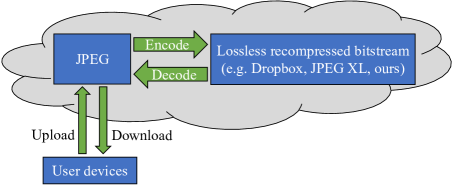
Figure 1: Lossless JPEG recompression is already adopted in real world (e.g. Dropbox Lepton [32]), saving storage without affecting the compatibility of JPEG on user side.

Several classical methods can be used to lossless compress JPEG images, e.g. Lepton [32] (already applied in Dropbox), JPEG XL [10, 11], and PAQ8PX [5], where the first two are designed for image compression while the last one for generic data compression.

Recently, learned lossless JPEG recompression has been studied using neural networks. Guo et al. [24] applies learning-based entropy model that operates on DCT domain to model data distribution and obtains about $30\%$ compression savings. Fan et al. [22] utilizes learned end-to-end lossy transform coding to reduce the redundancy of DCT coefficients in a compact representation domain and achieves about $21.49\%$ improvement. These two approaches have achieved superior compression savings on standard datasets than traditional methods, which shows the promise of learning-based JPEG recompression.

On the other hand, there are multiple subsampled formats in YCbCr colorspace for JPEG images, such as YCbCr 4:4:4 and YCbCr 4:2:0, namely the resolution of chroma components (i.e. Cb and Cr) is variable and may be equal to or $\frac{1}{4}$ of the luma component (i.e. Y). Current neural compressors, integrating these three color components along channel dimension as input, are incapable of supporting YCbCr 4:4:4 and YCbCr 4:2:0 using the same model. Another limitation is that their structure is not conducive to optimize throughput, which hinders real-world applications.

In this paper, we propose a more lightweight and flexible neural compressor composed of two neural networks, i.e. Y-Net and CbCr-Net in Figure 2, where Y-Net is used to compress luma component (i.e. Y) while CbCr-Net to chroma components (i.e. Cb and Cr). In this case, our compressor not only is compatible with a variety of JPEG formats, but also has higher computation efficiency due to luma and chroma being coded in parallel. We design two efficient context models for luma and chroma components respectively, namely pipeline parallel context model (PPCM) and compressed checkerboard context model (CCCM).

In conclusion, our contributions include:

• We propose a novel Multi-Level Parallel Conditional Modeling (ML-PCM) architecture for lossless JPEG recompression, which is compatible with various JPEG formats and enables parallel decoding in different granularities.

• Experiments show that ML-PCM achieves state-of-the-art performance on benchmark datasets with faster running speed (Table 1 and Table 2).

• ML-PCM can be extended to JPEG lossy compression and achieves significantly better RD performance than previous SOTA lossy compression method under higher bit rates (Figure 10).

• ML-PCM is designed to be friendly to multi-threading and streaming (Figure 9), reaching astonishing throughput after proper software optimization (Table 3), which can provide new insight for efficient learned image or video compression.

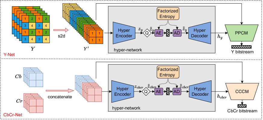
Figure 2: Overview of our Multi-Level Parallel Conditional Modeling (ML-PCM) architecture.

2 Related work

2.1 Overview of JPEG compression

JPEG first converts image from RGB sources to YCbCr colorspace and then selects a format for subsampling, including YCbCr 4:4:4, YCbCr 4:2:2, YCbCr 4:2:0 and so on. Subsequently, each component is divided into multiple $8\times 8$ blocks and each block is transformed by discrete cosine transform (DCT) into frequency coefficients (i.e. DCT coeficients). Specially, the coefficient with zero frequency is called DC coefficient while the remaining 63 coefficients are called AC coefficients. Next, these three color components are quantized by quantization tables to filter out information insensitive for human visual system, especially high frequencies and color details stored in chroma components. Finally, quantized coefficients are compressed by Huffman code with a probability model defined by Huffman tables.

2.2 JPEG recompression methods

Traditional. There are some traditional methods devoted to recompress JPEG images. Mozjpeg [3, 4] improves the encoder of JPEG to achieve smaller file size while maintaining compatibility with those already deployed JPEG decoders. It losslessly reduces file size by 10% on average for a sample of 1500 JPEG images from Wikimedia.

In addition, general data compression programs can also further compress JPEG images, such as PAQ8 [38] and CMIX [1]. PAQ8 is a series of compressor archivers, including famous PAQ8PX [5]. In fact, PAQ8PX is also adopted in CMIX. Though these compressors are different, they all employ a key technique called context mixing, where massive context models independently predict the next bit of input and then pick the most precise prediction for current step. Therefore, these methods achieve higher savings (about 23%), while they are considerably slower and consume more computation and memory.

Recently, more practical traditional compressors have emerged, e.g. Lepton [32] and JPEG XL [10, 11]. Lepton replaces Huffman code in JPEG with more efficient arithmetic code [59] and uses a sophisticated adaptive probability model which produces more accurate predictions. It achieves about 22% compression savings after recompressing JPEG losslessly. JPEG XL achieves further compression of JPEG file by extending the $8\times 8$ DCT to variable-size DCT, e.g. allowing block size to be one of 8, 16 or 32. And it uses ANS [19] in place of Huffman code.

Learning-based Guo et al. [24] directly learns a probability model by learning-based entropy model on DCT domain, which efficiently reduces the mismatch between estimated data distribution and true distribution. They achieve about 30% savings and outperform traditional compressors by a large margin. Fan et al. [22] points out that there exists considerable redundancy among DCT coefficients because discrete cosine transform is unable to eliminate redundant data adequately. They transform DCT coefficients into a compact representation by learned end-to-end lossy transform, and then code this representation and the residual between lossy recovery and original coefficients. They achieve about $21.49\%$ savings over JPEG.

However, these two methods use integrated color components as input and are incapable of supporting different JPEG subsample formats with single model. And their latency and throughput are not good enough for practical applications. Our multi-level parallel design is more effective and efficient, and is more compatible with software optimization techniques like multi-threading and streaming.

2.3 End-to-end lossless image compression

Actually, learned lossless JPEG recompression is a special use case of end-to-end lossless image compression. In theory, data can be compressed into bitstreams losslessly by entropy code with a probability model. According to Shannon’s source coding theory [52], the lower bound of the bitstream length is limited by the entropy of data’s ground truth distribution. However, the true distribution is unkown, entropy coder is generally applied with estimated distribution. Mismatch between the approximate distribution and the true distribution will bring overhead, i.e. the preciser the probability model is, the shorter the bitstream will be.

Recently, deep generative models (DGMs) have shown the powerful ability of approximating distribution. It is not surprising that many compression algorithms based on DGMs have emerged and obtain the recent state-of-the-art performance in terms of compression ratio. These algorithms can be roughly categorized into four groups: autoregressive model [16, 25, 44, 45, 48, 50, 56, 61] , variational autoencoder [23, 34, 36, 40, 51, 53, 54] , flow model [29, 31, 55, 58, 62] , and diffusion model [13, 30, 35]. Except for DGMs, some neural lossless compressor [15, 49, 60] uses context based entropy model for distribution approximation, which essentially is the improved variant of the autoregressive model in computational complexity. Moverover, some methods learn lossless compressor by compressing the residual of lossy compressors, such as [12, 41].

Those lossless compressors all operate on RGB domain and are designed to compress images stored in PNG format. According to Guo et al. [24], these methods are not effective when used to losslessly compress JPEG images. We provide an analysis to show that DCT domain is indeed preferred for JPEG lossless recompression.

3 Method

3.1 Overview

We apply the same data processing as Guo et al. [24] to rearrange each color component from $(h\times 8,w\times 8)$ to $(h,w,64)$. To support multiple subsampled formats, we design two independent networks for chroma components and luma component respectively in Figure 2. Each network is composed of a hyper-network (i.e. hyper encoder and hyper decoder) and a parallel context model (i.e. CCCM or PPCM), where hyper-network extracts side information to learn global correlation while context model captures more local details from decoded adjacent symbols to further reduce redundancy. The DCT coefficients of Y component is first transformed into $\bm{Y}^{\prime}$ by space-to-depth (s2d) and then compressed by Y-Net (top of Figure 2). Meanwhile, the DCT coefficients of Cb and Cr components are concatenated at channel dimension and compressed by CbCr-Net (bottom of Figure 2). Specifically, the hyper-network in Y-Net or CbCr-Net is simple and has similar structure as the hyperprior network in previous lossy compression methods [42] (detailed in the appendix), while CCCM and PPCM are novel and specially designed according to the traits of different color components, which is detailed in Section 3.3.

3.2 Why DCT domain is preferred?

Guo et al. [24] empirically shows that DCT domain brings superior performance than pixel domain. In this paper, we provide theoretical justification under mild assumption. Denote the image in pixel domain as $\bm{x}$, and its DCT transform coefficient as $\bm{w}=A\bm{x}$, and the quantized coefficient with quantization step-size $\Delta$ as $\bm{\tilde{w}}=\Delta\lfloor\bm{w}/\Delta\rceil$, where $\lfloor.\rceil$ is the rounding operator. We follow the $\rho$-domain assumption, which is commonly adopted in video coding [28]. More specifically, we assume that the bitrate to encode quantized symbol is proportional to the number of non-zero dimension after quantization. More formally, denote $R(\bm{\tilde{w}})$ as the bitrate to encode quantized symbol $\bm{\tilde{w}}$, we have:

$$\vspace{-0.5em}R(\bm{\tilde{w}})\propto(1-\rho(\bm{\tilde{w}}))\textrm{, where }\rho(\bm{\tilde{w}})=\sum_{i=1}^{D}\mathbbm{1}_{\bm{\tilde{w}}^{i}=0}$$ (1)

Denote the inversely transformed pixel domain symbols as $\bm{\tilde{x}}=A^{-1}\bm{\tilde{w}},$we have the following property:

$$\vspace{-0.5em}\rho(\bm{\tilde{x}})=\sum_{i=1}^{D}\mathbbm{1}_{\bm{\tilde{x}}^{i}=0}=\sum_{i=1}^{D}\mathbbm{1}_{\sum_{j=1}^{D}A^{ij}\bm{\tilde{w}}^{j}=0}$$ (2)

It is obvious that $\rho(\bm{\tilde{x}})<\rho(\bm{\tilde{w}})$, as $p(\sum_{j=1}^{D}A^{ij}\bm{\tilde{w}}^{j}=0)$ is very small, unless for very special $A$ such as identity matrix. Then, it becomes obvious that $R(\bm{\tilde{w}})<R(\bm{\tilde{x}})$, given the original quantization happens on $\bm{w}$ instead of $\bm{x}$. If we assume this conclusion on CABAC [39] (an ad-hoc entropy model) also applies to our entropy model, then we can say that the DCT-domain coding is preferred.

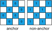
(a) Checkerboard [27]

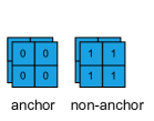
(b) CCCM

Figure 3: CCCM vs Checkerboard.

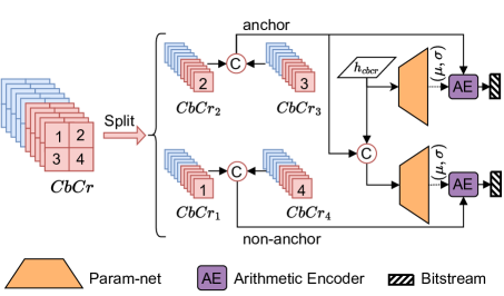
Figure 4: Compressing CbCr with CCCM and $\bm{h}_{cbcr}$. Param-net is detailed in the appendix.

Figure 5: Compressing Y with PPCM and $\bm{h}_{y}$. Param-net is detailed in the appendix.

3.3 Architecture

CCCM. He et al. [27] proposes a parallel context model with a two-pass decoding approach, where the symbol tensor is first decomposed into two groups (i.e. anchor and non-anchor in Figure 3(a)) by checkerboard-shaped mask, and then anchor serves as context of non-anchor to build conditional distribution. Although they eliminate the limitation of serial context model and speed up the decoding process, some redundant computation is involved because anchor and non-anchor use the same resolution as the symbol tensor. Therefore, we propose a compressed checkerboard context model (CCCM) for CbCr-Net by categorizing groups in a more compact way (Figure 3(b)). As shown in Figure 4, concatenated tensor of Cb and Cr is grouped into four groups $\bm{CbCr}_{i}$ ($i\in\left\{1,2,3,4\right\}$, denoting the location). Then, $\bm{CbCr}_{2}$ and $\bm{CbCr}_{3}$ are concatenated in the channel dimension as anchor , $\bm{CbCr}_{1}$ and $\bm{CbCr}_{4}$ as non-anchor. The anchor is compressed using a single Gaussian entropy model with mean and scale conditioned only on $\bm{h}_{cbcr}$ which is obtained by $\bm{\tilde{z}}_{cbcr}$ through the Hyper Decoder, while the entropy model for the non-anchor is conditioned on both $\bm{h}_{cbcr}$ and anchor.

PPCM. We propose a pipeline parallel context model (PPCM) to compress Y component, which enables more parallelism and less latency. As shown in Figure 5, $\bm{Y}^{\prime}$ (obtained by space-to-depth on $\bm{Y}$ ) is first split into matrix representation $\bm{y}^{(i)}_{j}$, $i\in\left\{1,2,3,4\right\}$ denotes row index, $j\in\left\{1,2,\dots,9\right\}$ denotes column index, and the lengths of each column $\bm{y}^{(i)}_{j}$ are set as 28, 8, 7, 6, 5, 4, 3, 2 and 1 respectively. Next, PPCM learns more powerful probability mass function (PMF) for each column using a single Gaussian entropy model with mean and scale conditioned on context and $\bm{h}_{y}$. Specially, the first block $\bm{y}^{(1)}_{1}$ is predicted only by $\bm{h}_{y}$ from the Hyper Decoder, while the entropy parameters for remaining columns in the first row (i.e. $\bm{y}^{(1)}_{j},j=2,3,\cdots,9$) are conditioned on all the decoded coefficients in previous columns ($\emph{i.e}.\hbox{}\left\{\bm{y}^{(1)}_{1},\cdots,\bm{y}^{(1)}_{j-1}\right\}$). The PMF for all columns in first row can be formulated as:

$$p\left(\bm{y}^{(1)}|\bm{\tilde{z}}\right)=\prod^{9}_{j=1}p\left(\bm{y}^{(1)}_{j}|\bm{C}^{(1)}\right)$$ (3)

$$p\left(\bm{y}^{(1)}_{j}|\bm{C}^{(1)}\right)=\prod^{m_{j}}_{k=1}p\left(\bm{y}^{(1)}_{jk}|\bm{C}^{(1)}\right)$$

$$p\left(\bm{y}^{(1)}_{jk}|\bm{C}^{(1)}\right)=\int_{\bm{y}^{(1)}_{jk}-\frac{1}{2}}^{\bm{y}^{(1)}_{jk}+\frac{1}{2}}\mathcal{N}(y^{\prime}|\mu_{\bm{y}^{(1)}_{jk}},b_{\bm{y}^{(1)}_{jk}})\,dy^{\prime}$$

where $\bm{C}^{(1)}=\left\{\bm{y}^{(1)}_{j-1},\cdots,\bm{y}^{(1)}_{1},\bm{\tilde{z}}\right\}$ denote the context for $\bm{y}^{(1)}_{j}$, $\bm{y}^{(1)}_{jk}$ is coefficient $k$ in column $j$ at first row $\bm{y}^{(1)}$, $m_{j}$ is the number of coefficients in column $j$, $j=1,2,\cdots,9$, and $k=1,2,\cdots,m_{j}$.

After first row is processed, they will be concatenated with $\bm{h}_{y}$ and then sent to a param-net network to acquire $\bm{prior}$ for $\bm{y}^{(2:4)}$. Unlike the strict processing order for columns in Guo et al. [24], the columns in $\bm{y}^{(2:4)}$ are conditioned on $\bm{prior}$ and previously decoded columns in a pipeline parallel manner. Specifically, entropy parameters of columns with same index $j$ (i.e. $\bm{y}^{(2:4)}_{j}$) can be calculated in parallel, and after these three context elements in column $j$ are compressed, they will be concatenated with $\bm{prior}$ and then sent to three param-net to obtain entropy parameters for $\bm{y}^{(2:4)}_{j+1}$. Repeat this operation until all columns in $\bm{y}^{(2:4)}$ are compressed. The calculation of PMF for all columns in $\bm{y}^{(2:4)}$ can be formulated as follows:

$$p\left(\bm{y}^{(2:4)}|\bm{y}^{(1)},\bm{\tilde{z}}\right)=\prod^{9}_{j=1}p\left(\bm{y}^{(2:4)}_{j}|\bm{C}^{(2)}\right)$$ (4)

$$p\left(\bm{y}^{(2:4)}_{j}|\bm{C}^{(2)}\right)$$

$$=p\left(\bm{y}^{(2)}_{j}|\bm{C}^{(2)}\right)p\left(\bm{y}^{(3)}_{j}|\bm{C}^{(2)}\right)p\left(\bm{y}^{(4)}_{j}|\bm{C}^{(2)}\right)$$

$$p\left(\bm{y}^{(i)}_{j}|\bm{C}^{(2)}\right)=\prod^{m_{j}}_{k=1}p\left(\bm{y}^{(i)}_{jk}|\bm{C}^{(2)}\right)$$

$$p\left(\bm{y}^{(i)}_{jk}|\bm{C}^{(2)}\right)=\int_{\bm{y}^{(i)}_{jk}-\frac{1}{2}}^{\bm{y}^{(i)}_{jk}+\frac{1}{2}}\mathcal{N}(y^{\prime}|\mu_{\bm{y}^{(i)}_{jk}},b_{\bm{y}^{(i)}_{jk}})\,dy^{\prime}$$

where $\bm{C}^{(2)}=\left\{\bm{y}_{j-1}^{(2:4)},\cdots,\bm{y}_{1}^{(2:4)},\bm{y}^{(1)},\bm{\tilde{z}}\right\}$ denote the context for $\bm{y}^{(2:4)}_{j}$, $\bm{y}^{(i)}_{jk}$ is coefficient $k$ in column $j$ at first row $\bm{y}^{(i)}$, $m_{j}$ is the number of coefficients in column $j$, $j=1,2,\cdots,9$, and $k=1,2,\cdots,m_{j}$.

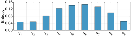
Figure 6: Entropy distribution along columns in Y-Net without shift context. $\bm{y}_{j}$ denotes total entropy of $\bm{y}_{j}^{(1:4)}$.

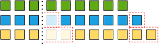
Figure 7: The shift context.

Shift Context. All coefficients in the same column of different rows (e.g. $\bm{y}^{(1:4)}_{j}$) represent the same frequency with different space location, while different columns in same rows (e.g. $\bm{y}^{(i)}_{1:9}$) represent different frequency with same space location. However, all columns in $\bm{y}^{(2:4)}$ rely on previous columns and are coded with same order, i.e. $\bm{y}^{(2:4)}_{1}\rightarrow\bm{y}^{(2:4)}_{2}\rightarrow\cdots\rightarrow\bm{y}^{(2:4)}_{9}$, which only explores the correlation across frequency. To exploit more correlation cross spatial dimension, we shift the coding order of columns in $\bm{y}^{(3)}$ and $\bm{y}^{(4)}$ to allow a subset of coefficients to learn from the coefficients at different space location in the same frequency, which is presented in Figure 7. As shown in Figure 6, entropy of the first three columns is much lower, which indicates that these columns have already been effectively compressed. Therefore, we shift the order from the fourth column, i.e. $\bm{y}^{(2:4)}_{1}\rightarrow\bm{y}^{(2:4)}_{2}\rightarrow\bm{y}^{(2:4)}_{3}\rightarrow\bm{y}^{(2)}_{4},\bm{y}^{(3)}_{5},\bm{y}^{(4)}_{6}\rightarrow\bm{y}^{(2)}_{5},\bm{y}^{(3)}_{6},\bm{y}^{(4)}_{7}\rightarrow\bm{y}^{(2)}_{6},\bm{y}^{(3)}_{7},\bm{y}^{(4)}_{8}\rightarrow\bm{y}^{(2)}_{7},\bm{y}^{(3)}_{8},\bm{y}^{(4)}_{9}\rightarrow\bm{y}^{(2)}_{8},\bm{y}^{(3)}_{9},\bm{y}^{(4)}_{4}\rightarrow\bm{y}^{(2)}_{9},\bm{y}^{(3)}_{4},\bm{y}^{(4)}_{5}$. Table 4 demonstrates that our Shift Context not only reduces FLOPs but also brings higher compression savings.

4 Experiments

Datasets. Following Guo et al. [24], we train our model on the largest 8000 images chosen from the ImageNet [17] validation set. We evaluate on four datasets, Kodak [37], DIV2K [8], CLIC [7] professional and CLIC mobile. We use torchjpeg.codec.quantize_at_quality [20] to extract quantized DCT coefficients with given JPEG quality level, and then feed these coefficients to model.

Implementation details. Training images are cropped randomly into $256\times 256$ patches and then quantized DCT coefficients are extracted. Y-Net and CbCr-Net are implemented in PyTorch [46] and optimized separately. We adopt Adam optimizer with learning-rate $10^{-4}$ and batch-size $16$. We apply gradient clipping (clip_max_norm = 0.5) for the sake of stability and decay learning rate to $10^{-5}$ for last 500 epochs. Y-Net is trained with three stages. We first train hyper-network to fully learn the global information, then train PPCM to capture detailed context, and finally finetune them together. Table 4 shows that Y-Net without three stage will deteriorate about 0.7% compression savings.

Deployment and software optimization. To better show the practicality of our method, We additionally deploy our model with TensorRT [2] library. We leverage 8-bit quantization [21] to further accelerate inference, which achieves comparable compression performance (only deteriorating about 1% savings for Y-Net and 0.7% for CbCr-Net) with the full precision model.

		BPP and Savings (%)
Source format	Method	Kodak	DIV2K	CLIC.mobile	CLIC.pro
JPEG 4:2:0	JPEG [57]	1.369	1.285	1.099	0.922
	Lepton [32]	1.102 $(19.50\%)$	1.017 $(20.86\%)$	0.863 $(21.47\%)$	0.701 $(23.97\%)$
	JPEG XL [10, 11]	1.173 $(14.30\%)$	1.072 $(16.58\%)$	0.908 $(17.38\%)$	0.744 $(19.30\%)$
	CMIX [1]	1.054 $(23.01\%)$	0.931 $(27.55\%)$	0.804 $(26.84\%)$	0.648 $(29.72\%)$
	Guo [24]	0.965 $(29.51\%)$	0.892 $(30.58\%)$	0.772 $(29.75\%)$	0.624 $(32.32\%)$
	Ours	0.959 $(29.96\%)$	0.887 $(31.0\%)$	0.755 $(31.32\%)$	0.608 $(34.06\%)$
JPEG 4:4:4	JPEG [57]	1.601	1.566	1.271	1.140
	Lepton [32]	1.261 $(21.27\%)$	1.220 $(22.10\%)$	0.964 $(24.11\%)$	0.844 $(25.98\%)$
	JPEG XL [10, 11]	1.348 $(15.81\%)$	1.272 $(18.78\%)$	1.013 $(20.28\%)$	0.881 $(22.70\%)$
	CMIX [1]	1.180 $(26.3\%)$	$--$	$--$	$--$
	Guo(dct444) [24]	1.122 $(29.90\%)$	1.088 $(30.54\%)$	0.888 $(30.14\%)$	0.769 $(32.59\%)$
	Ours	1.093 $(31.72\%)$	1.065 $(32.02\%)$	0.844 $(33.58\%)$	0.735 $(35.57\%)$

Table 1: Performance comparison on various datasets.

4.1 Performance

Performance comparison with other JPEG recompression methods. We compare the proposed model against other state-of-the-art methods for JPEG recompression on four test datasets mentioned above. Our model can not only be compatible with a variety of JPEG formats, but also achieve higher compression savings than previous SOTA. As shown in Table 1, with quality level set as 75, our method achieves lowest bit rate on all evaluation datasets and obtains around $30\%$ compression savings. Specially, for input in JPEG 4:4:4, CMIX is difficult to compress high resolution images (e.g. DIV2K, CLIC.mobile and CLIC.pro) beacuse of its high computation complexity.

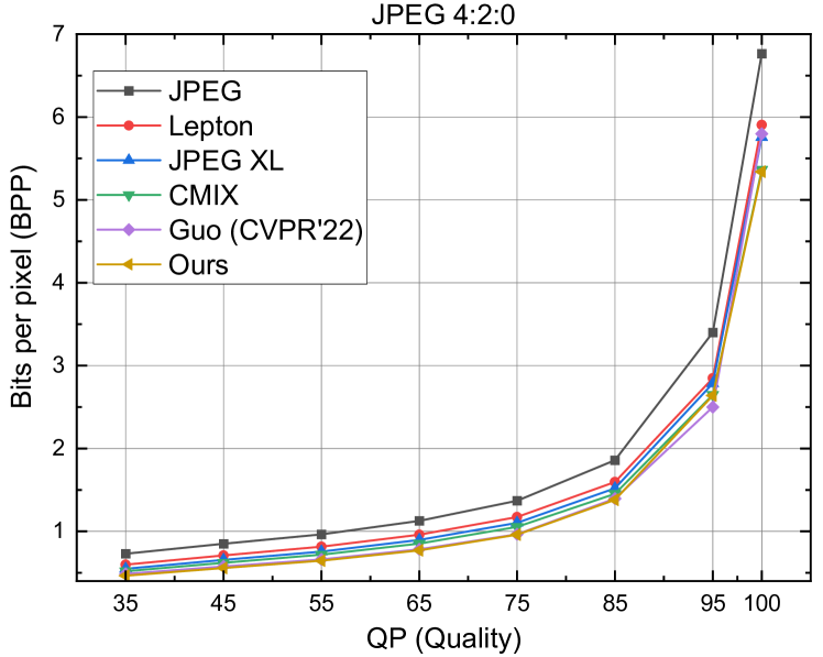
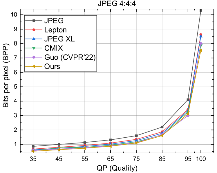
Figure 8: Comparison of bits per pixel (BPP) on Kodak dataset when recompressing JPEG images of different quality levels (QP). At QP$>85$, we use the model trained with mixed QP 96, 97, 98, 99 and 100. At other points, we use the model trained with QP 75.

Performance on different quality levels. We test our models on Kodak with two source formats at $8$ different JPEG quality levels (i.e. $quality=35,45,55,65,75,85,95,100$) in Figure 8. It shows that our method still outperforms other methods, which demonstrates our model, only using two sets of parameters, can well compress all quality levels including $QP>95$.

Network latency. Guo et al. [24] evaluated network latency of their model, L3C [40], IDF [31] and multi-scale [60], which shows their model is much faster. Table 2 shows that our model has achieved about 40% lower latency than Guo et al. [24] on decoding, even though our PyTorch implementation doesn’t do parallel optimization, i.e. all sub-models are computed in serial. Actually, we can achieve even lower latency with pipeline parallelism optimization. We compare the network operation with Guo et al. [24] during decompressing in Figure 9. All FLOPs in Guo et al. [24] have strict order and must be operated in serial. However, the FLOPs of Y-Net (in red box) and CbCr-Net in our model can be operated in parallel. Moreover, all FLOPs in PPCM for predicting columns $\bm{y}^{(2:4)}_{j}$ (in blue box) can be operated in parallel. Finally, our model’s operation ends at the red dotted line, while Guo et al. [24] at the purple dotted line.

Model	FLOPs	Latency (ms)
		Encode	Decode
Guo et al. [24]	136.11G	35.30	31.64
Ours	59.1G	22.52	18.98
Y-Net	30.84G	15.05	13.73
CbCr-Net	28.26G	7.46	5.25

Table 2: Comparison of network latency on Kodak dataset with JPEG 4:4:4 at QP 75. All results are test by PyTorch on single Nvidia GeForce GTX 1660 6GB (GPU).

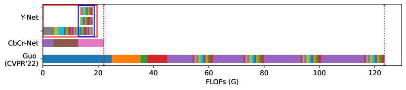
Figure 9: Comparison of network parallelism during decompressing. Horizontal bars (or rows) represent calculations executed on different pipelines, different colors represent different sub-modlues and length represents FLOPs per sub-modlue (evaluated on Kodak with JPEG 4:4:4 at QP 75). Our method is designed to be friendly to multi-threading and streaming.

Results of software optimization. As shown in Table 3, with proper software optimization, our method can obtain lower latency than JPEG XL, and achieves 57 FPS for 1080P images, which shows the promise of our method.

Model	device	Latency (ms)
		Encode	Decode
Lepton[32]	CPU	42.06	21.62
JPEG XL [10, 11]	CPU	52.79	68.50
CMIX [1]	CPU	4.1$\times 10^{5}$	4.2$\times 10^{5}$
Ours (int8)	GPU&CPU	52	54
Ours (fp16)	GPU&CPU	53	54
Model	device	Throughput (FPS)
		Encode	Decode
Lepton[32]	CPU	132.4	177.78
JPEG XL [10, 11]	CPU	103.09	141.64
Ours (int8)	GPU&CPU	57	57
Ours (fp16)	GPU&CPU	44.4	48

Table 3: Comparison of throughput and latency for 1080p images. CPU is Intel(R) Core(TM) i9-10900X CPU @ 3.70GHz and GPU is T4. Lepton (without decoding validation) and JPEG XL are tested on CPU with their optimal number of threads, i.e. 16 and 20 threads respectively. CMIX cannot set threads, so we use its default 1 thread. Our network inference runs on T4 GPU using TensorRT while entropy coder runs on CPU with 1 thread.

4.2 Comparison with lossy compression

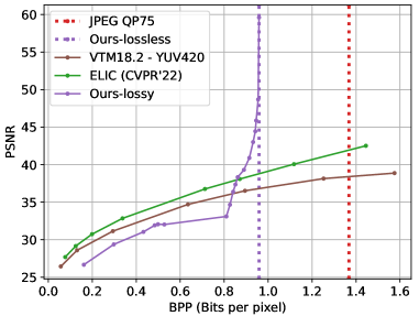
Figure 10: Comparison with lossy compression methods when taking JPEG images as input. The results are evaluated on Kodak with JPEG 4:2:0 at QP 75.

Lossy image compression focuses on the compression of images stored in lossless format like PNG, serving as replacement of JPEG. However, JPEG algorithm is more widely used in real application. If lossy compression methods are used to compress JPEG images, we will find an interesting discovery shown in Figure 10. For input images in JPEG format, after the bit rate exceeds a certain threshold, both learned (ELIC [26]) and non-learned (VTM, the latest intra coding from VVC/H.266 [43]) lossy compression methods reach higher bit rate than JPEG lossless recompression, and even higher than original JPEG file. In other words, lossy compression methods are not effective for JPEG lossy recompression under high bit rate.

We add some simple operations on DCT coefficients to make our method support lossy JPEG recompression without training. For example, for input DCT coefficients at QP 75, these coefficients are first dequantized, and then quantized again with quantization table at other QP, like QP 65 or QP 55 and so on. Then, the requantized coefficients are sent to our model and transcoded into bitstream. Finally, we achieve RD performance shown in purple solid line (marked as Ours-lossy) in Figure 10, which illustrates that this simple variant of our method can achieve significantly better RD performance than previous SOTA lossy compression method for JPEG input under higher bit rates, revealing the improvement space of lossy image compression.

4.3 Ablation study

PPCM. w/o ppcm drops the PPCM in Y-Net, which means there is only hyper-network to estimate the entropy parameters for Y component. Shown in Table 4, without PPCM, the bit rate of Y component increases severely (about 17%). Besides, w/ full parallel ppcm adapts PPCM into a fully parallel structure (more detailed architecture in appendix): $\bm{y}^{(1:4)}_{j}$ can be coded in parallel, and then be concatenated with $\bm{h}_{y}$ to help predicting next group. We find this variant deteriorates about 1.5% compression savings.

Method	Parameters	FLOPs	BPP
JPEG [57] (Y)	–	–	1.245
Y-Net	12.05M	30.84G	0.885
w/o ppcm	4.09M	6.434G	1.102
w/ full parallel ppcm	11.19M	28.19G	0.905
w/o shift context	12.08M	30.90G	0.892
w/o stage traning	12.05M	30.84G	0.894
JPEG [57] (Cb&Cr)	–	–	0.356
CbCr-Net	9.23M	28.26G	0.211
w/o cccm	4.20M	27.09G	0.248
w/ checkerboard	4.66M	38.21G	0.211

Table 4: Ablation study. We test a serial of models on Kodak with JPEG 4:4:4 at QP 75.

Shift Context. w/o shift context removes shift context from Y-Net. As shown in Table 4, we find shift context can not only further reduce about 0.56% bit rate , but also slightly save parameters and computation.

CCCM. Table 4 shows CCCM increases calculation slightly (about 1.17 GFLOPs), but helps chroma components reduce about 10% bit rate. We also replace CCCM with original checkerboard [27] and find checkerboard’s complexity is higher without compression benefits.

5 Conclusion

We propose a novel Multi-Level Parallel Conditional Modeling (ML-PCM) architecture for lossless recompression of existing JPEG images, which is compatible with various JPEG formats and achieves SOTA compression performance. Our model achieves at least 40% lower network latency than previous SOTA and reaches a good throughput after proper software optimization. Furthermore, for lossy JPEG recompression, a simple variant of our method obtains significantly better RD performance than previous SOTA lossy compression method in high bitrate.

References

- [1] Cmix. https://www.byronknoll.com/cmix.html.
- [2] Deep learning tensorrt documentation. https://docs.nvidia.com/deeplearning/tensorrt/.
- [3] Improved jpeg encoder. https://github.com/mozilla/mozjpeg.
- [4] Introducing the ‘mozjpeg’ project. https://research.mozilla.org/2014/03/05/introducing-the-mozjpeg-project/.
- [5] Paq8px compression archiver. https://github.com/hxim/paq8px.
- [6] W3techs - world wide web technology surveys. https://w3techs.com/.
- [7] Workshop and challenge on learned image compression. https://www.compression.cc/challenge/.
- [8] Eirikur Agustsson and Radu Timofte. Ntire 2017 challenge on single image super-resolution: Dataset and study. In Proceedings of the IEEE conference on computer vision and pattern recognition workshops, pages 126–135, 2017.
- [9] Nasir Ahmed, T_ Natarajan, and Kamisetty R Rao. Discrete cosine transform. IEEE transactions on Computers, 100(1):90–93, 1974.
- [10] Jyrki Alakuijala, Sami Boukortt, Touradj Ebrahimi, Evgenii Kliuchnikov, Jon Sneyers, Evgeniy Upenik, Lode Vandevenne, Luca Versari, and Jan Wassenberg. Benchmarking jpeg xl image compression. In Optics, Photonics and Digital Technologies for Imaging Applications VI, volume 11353, page 113530X. International Society for Optics and Photonics, 2020.
- [11] Jyrki Alakuijala, Ruud van Asseldonk, Sami Boukortt, Martin Bruse, Iulia-Maria Comșa, Moritz Firsching, Thomas Fischbacher, Evgenii Kliuchnikov, Sebastian Gomez, Robert Obryk, et al. Jpeg xl next-generation image compression architecture and coding tools. In Applications of Digital Image Processing XLII, volume 11137, page 111370K. International Society for Optics and Photonics, 2019.
- [12] Yuanchao Bai, Xianming Liu, Wangmeng Zuo, Yaowei Wang, and Xiangyang Ji. Learning scalable -constrained near-lossless image compression via joint lossy image and residual compression. arXiv preprint arXiv:2103.17015, 2021.
- [13] Tudor Barbu. Segmentation-based non-texture image compression framework using anisotropic diffusion models. Proceedings of the Romanian Academy, Series A: Mathematics, Physics, Technical Sciences, Information Science, 20(2):122–130, 2019.
- [14] Fabrice Bellard. Bpg image format. https://bellard.org/bpg.
- [15] Sheng Cao, Chao-Yuan Wu, and Philipp Krähenbühl. Lossless image compression through super-resolution. arXiv preprint arXiv:2004.02872, 2020.
- [16] Rewon Child, Scott Gray, Alec Radford, and Ilya Sutskever. Generating long sequences with sparse transformers. arXiv preprint arXiv:1904.10509, 2019.
- [17] Jia Deng, Wei Dong, Richard Socher, Li-Jia Li, Kai Li, and Li Fei-Fei. Imagenet: A large-scale hierarchical image database. In 2009 IEEE conference on computer vision and pattern recognition, pages 248–255. Ieee, 2009.
- [18] Jarek Duda. Asymmetric numeral systems: entropy coding combining speed of huffman coding with compression rate of arithmetic coding. arXiv preprint arXiv:1311.2540, 2013.
- [19] Jarek Duda, Khalid Tahboub, Neeraj J Gadgil, and Edward J Delp. The use of asymmetric numeral systems as an accurate replacement for huffman coding. In 2015 Picture Coding Symposium (PCS), pages 65–69. IEEE, 2015.
- [20] Max Ehrlich, Larry Davis, Ser-Nam Lim, and Abhinav Shrivastava. Quantization guided jpeg artifact correction. Proceedings of the European Conference on Computer Vision, 2020.
- [21] Steven K Esser, Jeffrey L McKinstry, Deepika Bablani, Rathinakumar Appuswamy, and Dharmendra S Modha. Learned step size quantization. In International Conference on Learning Representations, 2020.
- [22] Xiaoshuai Fan, Xin Li, and Zhibo Chen. Learned lossless jpeg transcoding via joint lossy and residual compression. arXiv preprint arXiv:2208.11673, 2022.
- [23] Gergely Flamich, Marton Havasi, and José Miguel Hernández-Lobato. Compressing images by encoding their latent representations with relative entropy coding. Advances in Neural Information Processing Systems, 33:16131–16141, 2020.
- [24] Lina Guo, Xinjie Shi, Dailan He, Yuanyuan Wang, Rui Ma, Hongwei Qin, and Yan Wang. Practical learned lossless jpeg recompression with multi-level cross-channel entropy model in the dct domain. In Proceedings of the IEEE/CVF Conference on Computer Vision and Pattern Recognition (CVPR), pages 5862–5871, June 2022.
- [25] Curtis Hawthorne, Andrew Jaegle, Catalina Cangea, Sebastian Borgeaud, Charlie Nash, Mateusz Malinowski, Sander Dieleman, Oriol Vinyals, Matthew M. Botvinick, Ian Simon, Hannah Sheahan, Neil Zeghidour, Jean-Baptiste Alayrac, João Carreira, and Jesse H. Engel. General-purpose, long-context autoregressive modeling with perceiver AR. In ICML, volume 162 of Proceedings of Machine Learning Research, pages 8535–8558. PMLR, 2022.
- [26] Dailan He, Ziming Yang, Weikun Peng, Rui Ma, Hongwei Qin, and Yan Wang. Elic: Efficient learned image compression with unevenly grouped space-channel contextual adaptive coding. In Proceedings of the IEEE/CVF Conference on Computer Vision and Pattern Recognition, pages 5718–5727, 2022.
- [27] Dailan He, Yaoyan Zheng, Baocheng Sun, Yan Wang, and Hongwei Qin. Checkerboard context model for efficient learned image compression. In Proceedings of the IEEE/CVF Conference on Computer Vision and Pattern Recognition, pages 14771–14780, 2021.
- [28] Zhihai He and Chang Wen Chen. [rho]-domain optimum bit allocation and accurate rate control for DCT video coding. In C.-C. Jay Kuo, editor, Visual Communications and Image Processing 2002, volume 4671, pages 734 – 745. International Society for Optics and Photonics, SPIE, 2002.
- [29] Jonathan Ho, Evan Lohn, and Pieter Abbeel. Compression with flows via local bits-back coding. Advances in Neural Information Processing Systems, 32:3879–3888, 2019.
- [30] Emiel Hoogeboom, Alexey A Gritsenko, Jasmijn Bastings, Ben Poole, Rianne van den Berg, and Tim Salimans. Autoregressive diffusion models. arXiv preprint arXiv:2110.02037, 2021.
- [31] Emiel Hoogeboom, Jorn Peters, Rianne van den Berg, and Max Welling. Integer discrete flows and lossless compression. Advances in Neural Information Processing Systems, 32:12134–12144, 2019.
- [32] Daniel Reiter Horn, Ken Elkabany, Chris Lesniewski-Laas, and Keith Winstein. The design, implementation, and deployment of a system to transparently compress hundreds of petabytes of image files for a file-storage service. In Proceedings of the 14th USENIX Conference on Networked Systems Design and Implementation, pages 1–15, 2017.
- [33] David A Huffman. A method for the construction of minimum-redundancy codes. Proceedings of the IRE, 40(9):1098–1101, 1952.
- [34] Ning Kang, Shanzhao Qiu, Shifeng Zhang, Zhenguo Li, and Shu-Tao Xia. Pilc: Practical image lossless compression with an end-to-end gpu oriented neural framework. In Proceedings of the IEEE/CVF Conference on Computer Vision and Pattern Recognition, pages 3739–3748, 2022.
- [35] Diederik Kingma, Tim Salimans, Ben Poole, and Jonathan Ho. Variational diffusion models. Advances in neural information processing systems, 34:21696–21707, 2021.
- [36] Friso Kingma, Pieter Abbeel, and Jonathan Ho. Bit-swap: Recursive bits-back coding for lossless compression with hierarchical latent variables. In International Conference on Machine Learning, pages 3408–3417. PMLR, 2019.
- [37] Eastman Kodak. Kodak lossless true color image suite (photocd pcd0992). http://r0k.us/graphics/kodak/, 1993.
- [38] Matt Mahoney. Data compression programs. http://mattmahoney.net/dc/.
- [39] D. Marpe, H. Schwarz, and T. Wiegand. Context-based adaptive binary arithmetic coding in the h.264/avc video compression standard. IEEE Transactions on Circuits and Systems for Video Technology, 13(7):620–636, 2003.
- [40] Fabian Mentzer, Eirikur Agustsson, Michael Tschannen, Radu Timofte, and Luc Van Gool. Practical full resolution learned lossless image compression. In Proceedings of the IEEE/CVF conference on computer vision and pattern recognition, pages 10629–10638, 2019.
- [41] Fabian Mentzer, Luc Van Gool, and Michael Tschannen. Learning better lossless compression using lossy compression. In Proceedings of the IEEE/CVF Conference on Computer Vision and Pattern Recognition, pages 6638–6647, 2020.
- [42] David Minnen, Johannes Ballé, and George D Toderici. Joint autoregressive and hierarchical priors for learned image compression. In Advances in Neural Information Processing Systems, pages 10771–10780, 2018.
- [43] Jens-Rainer Ohm and Gary J Sullivan. Versatile video coding–towards the next generation of video compression. In Picture Coding Symposium, volume 2018, 2018.
- [44] Aäron van den Oord, Nal Kalchbrenner, Oriol Vinyals, Lasse Espeholt, Alex Graves, and Koray Kavukcuoglu. Conditional image generation with pixelcnn decoders. In Proceedings of the 30th International Conference on Neural Information Processing Systems, pages 4797–4805, 2016.
- [45] Niki Parmar, Ashish Vaswani, Jakob Uszkoreit, Lukasz Kaiser, Noam Shazeer, Alexander Ku, and Dustin Tran. Image transformer. In International conference on machine learning, pages 4055–4064. PMLR, 2018.
- [46] Adam Paszke, Sam Gross, Francisco Massa, Adam Lerer, James Bradbury, Gregory Chanan, Trevor Killeen, Zeming Lin, Natalia Gimelshein, Luca Antiga, et al. Pytorch: An imperative style, high-performance deep learning library. In Advances in Neural Information Processing Systems, pages 8024–8035, 2019.
- [47] Majid Rabbani. Jpeg2000: Image compression fundamentals, standards and practice. Journal of Electronic Imaging, 11(2):286, 2002.
- [48] Scott Reed, Aäron Oord, Nal Kalchbrenner, Sergio Gómez Colmenarejo, Ziyu Wang, Yutian Chen, Dan Belov, and Nando Freitas. Parallel multiscale autoregressive density estimation. In International Conference on Machine Learning, pages 2912–2921. PMLR, 2017.
- [49] Hochang Rhee, Yeong Il Jang, Seyun Kim, and Nam Ik Cho. Lc-fdnet: Learned lossless image compression with frequency decomposition network. In Proceedings of the IEEE/CVF Conference on Computer Vision and Pattern Recognition, pages 6033–6042, 2022.
- [50] Aurko Roy, Mohammad Saffar, Ashish Vaswani, and David Grangier. Efficient content-based sparse attention with routing transformers. Transactions of the Association for Computational Linguistics, 9:53–68, 2021.
- [51] Tom Ryder, Chen Zhang, Ning Kang, and Shifeng Zhang. Split hierarchical variational compression. In Proceedings of the IEEE/CVF Conference on Computer Vision and Pattern Recognition, pages 386–395, 2022.
- [52] Shannon and E. C. A mathematical theory of communication. Bell Systems Technical Journal, 27(4):623–656, 1948.
- [53] James Townsend, Thomas Bird, and David Barber. Practical lossless compression with latent variables using bits back coding. In International Conference on Learning Representations, 2018.
- [54] James Townsend, Thomas Bird, Julius Kunze, and David Barber. Hilloc: Lossless image compression with hierarchical latent variable models. arXiv preprint arXiv:1912.09953, 2019.
- [55] Rianne van den Berg, Alexey A Gritsenko, Mostafa Dehghani, Casper Kaae Sønderby, and Tim Salimans. Idf++: Analyzing and improving integer discrete flows for lossless compression. In International Conference on Learning Representations, 2020.
- [56] Aaron Van Oord, Nal Kalchbrenner, and Koray Kavukcuoglu. Pixel recurrent neural networks. In International Conference on Machine Learning, pages 1747–1756. PMLR, 2016.
- [57] Gregory K Wallace. The jpeg still picture compression standard. IEEE transactions on consumer electronics, 38(1):xviii–xxxiv, 1992.
- [58] Siyu Wang, Jianfei Chen, Chongxuan Li, Jun Zhu, and Bo Zhang. Fast lossless neural compression with integer-only discrete flows. In International Conference on Machine Learning, pages 22562–22575. PMLR, 2022.
- [59] Ian H. Witten, Radford M. Neal, and John G. Cleary. Arithmetic coding for data compression. Commun. ACM, 30(6):520–540, June 1987.
- [60] Honglei Zhang, Francesco Cricri, Hamed R Tavakoli, Nannan Zou, Emre Aksu, and Miska M Hannuksela. Lossless image compression using a multi-scale progressive statistical model. In Proceedings of the Asian Conference on Computer Vision, 2020.
- [61] Mingtian Zhang, Andi Zhang, and Steven McDonagh. On the out-of-distribution generalization of probabilistic image modelling. In NeurIPS, pages 3811–3823, 2021.
- [62] Shifeng Zhang, Chen Zhang, Ning Kang, and Zhenguo Li. ivpf: Numerical invertible volume preserving flow for efficient lossless compression. In Proceedings of the IEEE/CVF Conference on Computer Vision and Pattern Recognition, pages 620–629, 2021.