Learn With Imagination:
Safe Set Guided State-wise Constrained Policy Optimization

Abstract

Deep reinforcement learning (RL) excels in various control tasks, yet the absence of safety guarantees hampers its real-world applicability. In particular, explorations during learning usually results in safety violations, while the RL agent learns from those mistakes. On the other hand, safe control techniques ensure persistent safety satisfaction but demand strong priors on system dynamics, which is usually hard to obtain in practice. To address these problems, we present Safe Set Guided State-wise Constrained Policy Optimization (S-3PO), a pioneering algorithm generating state-wise safe optimal policies with zero training violations, i.e., learning without mistakes. S-3PO first employs a safety-oriented monitor with black-box dynamics to ensure safe exploration. It then enforces a unique cost for the RL agent to converge to optimal behaviors within safety constraints. S-3PO outperforms existing methods in high-dimensional robotics tasks, managing state-wise constraints with zero training violation. This innovation marks a significant stride towards real-world safe RL deployment.

1 Introduction

Reinforcement Learning (RL) has showcased remarkable advancements in domains like control and games. However, its focus on reward maximization sometimes neglects safety, potentially leading to catastrophic outcomes (Gu et al. 2022). To rectify this, the concept of safe RL emerged, aiming to ensure safety throughout or after training. Initial endeavors centered on Constrained Markov Decision Processes, often emphasizing cumulative or chance constraints (Ray, Achiam, and Amodei 2019; Achiam et al. 2017; Liu, Halev, and Liu 2021). While effective, these approaches lack instantaneous safety guarantees, which is crucial for managing emergencies like collision avoidance in autonomous vehicles (Zhao et al. 2023c; He et al. 2023). Recent strides (Zhao et al. 2023b) leveraged the Maximum Markov Decision Process to ensure instantaneous safety by bounding violations while integrating trust region techniques for policy enhancement, resulting in simultaneous improvement of worst-case performance and adherence to cost constraints. However, these approaches still cannot ensure safety during learning due to potentially unsafe explorative behaviors.

Meanwhile, safe control methods to continuously meet stringent safety requirements in predictable environments are widely examined, with energy function-based methods being the most prevalent (Khatib 1986; Ames, Grizzle, and Tabuada 2014; Liu and Tomizuka 2014; Gracia, Garelli, and Sala 2013; Wei and Liu 2019). These methods establish energy functions assigning lower energy to safe states and project nominal control into energy dissipating control, hence persistently maintaining system safety. However, these approahces heavily rely on accessible white-box analytical models of system dynamics. The Implicit Safe Set Algorithm (ISSA) (Zhao, He, and Liu 2021) addresses this problem using black-box optimization over black-box dynamics models. Nevertheless, this method involves complex computation to monitor the RL policy and there is no guarantee that the RL policy itself learns to behave safely. These hamper the suitability of the algorithm for real-time safety critical applications.

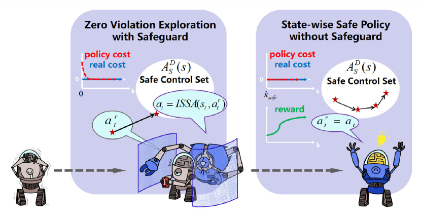
Figure 1: Overview of the principles of the S-3PO algorithm.

In summary, a pressing need arises for a method leveraging both the zero-training-time-violation ability of safe control and optimal convergence of safe RL. To bridge this gap, we introduce a novel Safe Set Guided State-wise Constrained Policy Optimization (S-3PO) algorithm. S-3PO safeguards the exploration of immature policies with a black-box safe control method and derives a novel formulation where RL learns an optimal safe policy by constraining the state-wise “imaginary" safety violations. An overview of the prescribed S-3PO principles is presented in Figure 1. Empirical validation underscores S-3PO’s efficacy in training neural network policies encompassing thousands of parameters for high-dimensional simulated robot locomotion tasks. Our contribution marks a substantial advancement in the realm of practical safe RL algorithms, poised to find applications in a multitude of real-world challenges.

2 Problem Formulation

2.1 Preliminaries

Dynamics

We consider a robot system described by its state $s_{t}\in\mathcal{S}\subset\mathbb{R}^{n_{s}}$ at time step $t$, with $n_{s}$ denoting the dimension of the state space $\mathcal{S}$, and its action input $a_{t}\in\mathcal{A}\subset\mathbb{R}^{n_{a}}$ at time step $t$, where $n_{a}$ represents the dimension of the control space $\mathcal{A}$. The system dynamics are defined as follows:

$$\begin{split}&s_{t+1}=f(s_{t},a_{t}),\\ \end{split}$$ (1)

where $f:\mathcal{S}\times\mathcal{A}\rightarrow\mathcal{S}$ is a deterministic function that maps the current robot state and control to the robot’s state in the next time step.

To maintain simplicity, our approach focuses on deterministic dynamics, although it is worth noting that the proposed method can be readily extended to accommodate stochastic dynamics (Zhao, He, and Liu 2021; Noren, Zhao, and Liu 2021). Additionally, we assume the access to the dynamics model $f$ is only in the training phase, and is restricted to an implicit black-box form, as exemplified by an implicit digital twin simulator or a deep neural network model (Zhao, He, and Liu 2021). We also assume there is no model mismatch, while model mismatch can be addressed by robust safe control (Wei et al. 2022) and is left for future work. Post training, the knowledge of the dynamics model is concealed, aligning with practical scenarios where digital twins of real-world environments are too costly to access during model deployment.

Markov Decision Process

In this research, our primary focus lies in ensuring safety for episodic tasks, which falls within the purview of finite-horizon Markov Decision Processes (MDP). An MDP is defined by a tuple $(\mathcal{S},\mathcal{A},\gamma,R,P,\mu)$. The reward function is denoted by $R:\mathcal{S}\times\mathcal{A}\mapsto\mathbb{R}$, the discount factor by $0\leq\gamma<1$, the initial state distribution by $\mu:\mathcal{S}\mapsto\mathbb{R}$, and the transition probability function by $P:\mathcal{S}\times\mathcal{A}\times\mathcal{S}\mapsto\mathbb{R}$.

The transition probability $P(s^{\prime}|s,a)$ represents the likelihood of transitioning to state $s^{\prime}$ when the previous state was $s$, and the agent executed action $a$ at state $s$. This paper assumes deterministic dynamics, implying that $P(s_{t+1}|s_{t},a_{t})=1$ when $s_{t+1}=f(s_{t},a_{t})$. We denote the set of all stationary policies as $\Pi$, and we further denote $\pi_{\theta}$ as a policy parameterized by the parameter $\theta$.

In the context of an MDP, our ultimate objective is to learn a policy $\pi$ that maximizes a performance measure $\mathcal{J}(\pi)$, computed via the discounted sum of rewards, as follows:

$$\mathcal{J}(\pi)=\mathbb{E}_{\tau\sim\pi}\left[\sum_{t=0}^{H}\gamma^{t}R(s_{t},a_{t},s_{t+1})\right],$$ (2)

where $H\in\mathbb{N}$ denotes the horizon, $\tau=[s_{0},a_{0},s_{1},\cdots]$, and $\tau\sim\pi$ indicates that the distribution over trajectories depends on $\pi$, i.e., $s_{0}\sim\mu$, $a_{t}\sim\pi(\cdot|s_{t})$, and $s_{t+1}\sim P(\cdot|s_{t},a_{t})$.

Safety Specification

The safety specification requires that the system state remains within a closed subset in the state space, denoted as the “safe set” $\mathcal{S}_{S}$. This safe set is defined by the zero-sublevel set of a continuous and piecewise smooth function $\phi_{0}:\mathbb{R}^{n_{s}}\rightarrow\mathbb{R}$, where $\mathcal{S}_{S}=\{s\mid\phi_{0}(s)\leq 0\}$. Users directly specify both $\mathcal{S}_{S}$ and $\phi_{0}$, which is easy to specify. For instance, for collision avoidance, $\phi_{0}$ can be specified as the negative closest distance between the robot and environmental obstacles.

2.2 Problem

We are interested in the safety imperative of averting collisions for mobile robots navigating 2D planes. We aim to persistently satisfy safety specifications at every time step while solving MDP, following the intuition of State-wise Constrained Markov Decision Process (SCMDP) (Zhao et al. 2023c). Formally, the set of feasible stationary policies for SCMDP is defined as

$$\bar{\Pi}_{C}=\{\pi\in\Pi\big{|}~{}\forall s_{t}\sim\tau,s_{t}\in\mathcal{S}_{S}\},$$ (3)

where $\tau\sim\pi$. Then, the objective for SCMDP is to find a feasible stationary policy from $\bar{\Pi}_{C}$ that maximizes the performance measure. Formally,

$$\max_{\theta}\mathcal{J}(\pi_{\theta}),\text{ s.t. }\pi_{\theta}\in\bar{\Pi}_{C}.$$ (4)

State-wise Safe Policy with Zero Violation Training

The primary focus of this paper centers on solving (4), i.e., ensuring no safety violation during the training process, while achieving convergence of the policy to the optimal solution of (4).

3 Prior Works

3.1 Safe Reinforcement Learning

Existing safe RL approaches either consider safety after convergence or safety during training (Zhao et al. 2023c). End-to-end approaches are usually used to ensure safety after convergence (Liang, Que, and Modiano 2018; Tessler, Mankowitz, and Mannor 2018; Bohez et al. 2019; Ma et al. 2021; He, Zhao, and Liu 2023). However, these approaches cannot avoid unsafe explorations. Safety in training is achieved by hierarchical approaches which uses a safeguard to filter out unsafe explorative actions. The safeguard relies on the knowledge on the system dynamics, which can be either learned dynamics (Dalal et al. 2018; Thananjeyan et al. 2021; Zhao, He, and Liu 2022), white-box dynamics (Fisac et al. 2018; Shao et al. 2021), or black-box dynamics (Zhao, He, and Liu 2021). Nevertheless, these methods cannot guarantee convergence of the RL policy.

The proposed approach is the first to address safety both during training and after convergence, which can potentially serve as a general framework to bridge these two types of approaches. In the following, we choose the most advanced method in each category to form the proposed approach, so that it relies on the least assumptions.

3.2 Implicit Safe Set Algorithm

Energy function-based methods  (Wei and Liu 2019) achieve safe control by designing an energy function offline such that 1) the low energy states are safe and 2) there always exists a feasible control input to dissipate the energy. A typical design (Liu and Tomizuka 2014) was proposed as $\phi=\phi_{0}^{*}+k_{1}\dot{\phi}_{0}+\cdots+k_{n}\phi_{0}^{(n)}$. It is shown in (Liu and Tomizuka 2014) that if the control input is unbounded ($\mathcal{A}=\mathbb{R}^{n_{a}}$), then there always exist a control input that satisfies the constraint $\dot{\phi}\leq 0\text{ when }\phi=0$; and if the control input always satisfies that constraint, then the set $\bar{\mathcal{S}}:=\{s\mid\phi(s)\leq 0\}\cap\{s\mid\phi_{0}(s)\leq 0\}$ is forward invariant. In practice, the actual control signal is computed through a quadratic projection of the nominal control $a^{r}$ to the control constraint

$$a= \mathop{\mathbf{argmin}}_{a\in\mathcal{A}}\|a-a^{r}\|^{2}\text{ s.t. }\dot{\phi}\leq-\eta(\phi),$$ (5)

where $\eta(\phi)$ is designed to be a positive constant when $\phi\geq 0$ and $-\infty$ when $\phi<0$ according to SSA (Liu and Tomizuka 2014). Here, we define the set of safe control as $\mathcal{A}_{S}(s):=\{a\in\mathcal{A}\mid\dot{\phi}\leq-\eta(\phi)\}$. To match the notion of MDP, we should consider discrete-time safe control set $\mathcal{A}_{S}^{D}(s):=\{a\in\mathcal{A}\mid\phi(f(s,a))\leq\max\{\phi(s)-\eta,0\}\}$.

Based on these, the implicit safe set algorithm (ISSA) (Zhao, He, and Liu 2021) was proposed to construct the black-box dynamics based safeguard ensuring persistent satisfication of safety specification. The black-box dynamics can be a digital twin or neural network. Under some mild assumptions, it first synthesizes a safety index to make sure $\mathcal{A}_{S}(s)$ is nonempty for all $s$ (details of the mild assumptions and safety index synthesis are summarized in Appendix A). Then it manages to project the reference action generated from RL policy $\pi_{\theta}$ into $\mathcal{A}_{S}(s)$ during policy training. In detail, the nominal control $a_{t}^{r}$ needs to be projected to $\mathcal{A}_{S}^{D}(s_{t})$ by solving the following optimization:

$$\begin{split}&\min_{a_{t}\in\mathcal{A}}\|a_{t}-a^{r}_{t}\|^{2}\\ &\text{s.t. }\phi(f(s_{t},a_{t}))\leq\max\{\phi(s_{t})-\eta,0\}.\end{split}$$ (6)

To solve (6), they first introduce a sample-efficient Adaptive Momentum Boundary Approximation (AdamBA) algorithm. Then, ISSA directly uses it to find the safe control with minimum deviation from the reference control along the boundaries of $\mathcal{A}_{S}^{D}(s)$. If the process fails to return a solution, grid sampling will be deployed to find a safe control; and AdamBA is deployed again to improve the solution optimality with respect to (6). We summarize details of AdamBA and ISSA in Algorithm 2 and Algorithm 3, respectively.

3.3 State-wise Constrained Policy Optimization

Safe RL algorithms under the framework of Constrained Markov Decision Process (CMDP) do not consider state-wise constraints. To address this gap, State-wise Constrained Policy Optimization (SCPO) was proposed (Zhao et al. 2023b) to provide guarantees for state-wise constraint satisfaction in expectation, which is under the framework of State-wise CMDP (SCMDP). To achieve this, SCPO directly constrain the expected maximum state-wise cost along the trajectory. And they introduced Maximum MDP (MMDP). In this setup, a running maximum cost value is associated with each state, and a non-discounted finite MDP is utilized to track and accumulate non-negative increments in cost. The format of MMDP will be introduced in Section 4.

4 Safety Index Guided State-wise Constrained Policy Optimization

The core idea of S-3PO is to enforce zero safety violation during training by projecting unsafe actions to the safe set, and then constrain the "imaginary" safety violation (i.e., what if the projection is not done) to ensure convergence of the policy to an optimal safe policy.

Zero Violation Exploration

To ensure zero violation exploration, we safeguard nominal control via solving (6) at every time step during policy training. In this paper, we adopt ISSA to solve (6). For the 2D collision avoidance problem considered in this paper, we choose the same safety index synthesis rule as [Section 4.1, (Zhao, He, and Liu 2021)], which is summarized in Appendix A. We show in Section 6 that with the safety index synthesis rule, ISSA is guaranteed to find a feasible solution of (6), making the system forward invariance in the set $\mathcal{\bar{S}}$.

Learning Safety Measures Safely

While eliminating safety violations during training is good, this also brings inevitable challenges for the policy learning as it directly eliminates the unsafe experience, making the policy unable to distinguish between safe and unsafe actions. To overcome this challenge, the main intuition we have is that instead of directly experiencing unsafe states, i.e. $s\notin\mathcal{S}_{S}$, policy can learn to act safely from “imagination", i.e., how unsafe it will be if the safeguard had not been triggered? The critical observation we rely upon is that:

Observation 1.

Define $\Delta\phi_{t}=\Delta\phi(s_{t},a_{t},s_{t+1})\doteq\phi(f(s_{t},a^{r}_{t}))-\phi(f(s_{t},a_{t}))$, i.e. the degree of required correction to safeguard $a_{t}^{r}$. Therefore, $\Delta\phi_{t}$ can be treated as an imagination on how unsafe the reference action would be, where $\Delta\phi_{t}\leq 0$ means $a_{t}^{r}\in\mathcal{A}_{S}^{D}(s_{t})$.

Following 1, Equation 4 can be translated to:

$$\max_{\theta}\mathcal{J}(\pi_{\theta}),\text{ s.t. }\pi_{\theta}\in\{\pi\in\Pi\big{|}~{}\forall\Delta\phi_{t}\sim\tau,\Delta\phi_{t}\leq 0\}.$$ (7)

Remark 1.

Policies satisfying (7) ensure there is no imaginary safety violation for any possible $a_{t}^{r}$, making $\pi_{\theta}$ a safe policy as required by (4).

Transfrom State-wise Constraint into Maximum Constraint

For (7), each state-action transition pair corresponds to a constraint, which is intractable to solve. Inspired by (Zhao et al. 2023c), we constrain the expected maximum state-wise $\Delta\phi$ along the trajectory instead of individual state-action transition $\Delta\phi$.

Next, by treating $\Delta\phi_{t}$ as an “imaginary” cost, we define a MMDP (Zhao et al. 2023c) by introducing (i) an up-to-now maximum state-wise cost $M$ within $\mathcal{M}\subset\mathbb{R}$, and (ii) a "cost increment" function $D$, where $D:(\mathcal{S},\mathcal{M})\times\mathcal{A}\times\mathcal{S}\mapsto[0,\mathbb{R}^{+}]$ maps the augmented state-action transition tuple to non-negative cost increments. We define the augmented state $\hat{s}=(s,M)\in(\mathcal{S},\mathcal{M})\doteq\hat{{\mathcal{S}}}$, where $\hat{{\mathcal{S}}}$ is the augmented state space. Formally,

$$D\big{(}\hat{s}_{t},a_{t},\hat{s}_{t+1}\big{)}=\max\{\Delta\phi(s_{t},a_{t},s_{t+1})-M,0\}.$$ (8)

By setting $D\big{(}\hat{s}_{0},a_{0},\hat{s}_{1}\big{)}=\Delta\phi(s_{0},a_{0},s_{1})$, we have $M=\sum_{k=0}^{t-1}D\big{(}\hat{s}_{k},a_{k},\hat{s}_{k+1}\big{)}$ for $t\geq 1$. Hence, we define expected maximum state-wise cost (or $D$-return) for $\pi$:

$$\mathcal{J}_{D}(\pi)=\mathbb{E}_{\tau\thicksim\pi}\Bigg{[}\sum_{t=0}^{H}D\big{(}\hat{s}_{t},a_{t},\hat{s}_{t+1}\big{)}\Bigg{]}.$$ (9)

With (9), (7) can be rewritten as:

$$\mathop{\underset{\pi}{\mathop{\mathbf{max}}}}\mathcal{J}(\pi),~{}\mathop{\mathbf{s.t.}}\mathcal{J}_{D}(\pi)\leq 0,$$ (10)

where $\mathcal{J}(\pi)=\mathbb{E}_{\tau\sim\pi}\left[\sum_{t=0}^{H}\gamma^{t}R(\hat{s}_{t},a_{t},\hat{s}_{t+1})\right]$ and $R(\hat{s},a,\hat{s}^{\prime})\doteq R(s,a,s^{\prime})$. With $R(\tau)$ being the discounted return of a trajectory, we define the on-policy value function as $V^{\pi}(\hat{s})\doteq\mathbb{E}_{\tau\sim\pi}[R(\tau)|\hat{s}_{0}=\hat{s}]$, the on-policy action-value function as $Q^{\pi}(\hat{s},a)\doteq\mathbb{E}_{\tau\sim\pi}[R(\tau)|\hat{s}_{0}=\hat{s},a_{0}=a]$, and the advantage function as $A^{\pi}(\hat{s},a)\doteq Q^{\pi}(\hat{s},a)-V^{\pi}(\hat{s})$. Lastly, we define on-policy value functions, action-value functions, and advantage functions for the cost increments in analogy to $V^{\pi}$, $Q^{\pi}$, and $A^{\pi}$, with $D$ replacing $R$, respectively. We denote those by $V_{D}^{\pi}$, $Q_{D}^{\pi}$ and $A_{D}^{\pi}$.

Remark 2.

Equation 7 is difficult to solve since there are as many constraints as the size of trajectory $\tau$. With (10), we turn all constraints in (7) into only a single constraint on the maximal $\Delta\phi$ along the trajectory, yielding a practically solvable problem.

S-3PO

To solve (10), we propose S-3PO inspired by recent trust region optimization methods (Schulman et al. 2015). S-3PO uses KL divergence distance to restrict the policy search in (10) within a trust region around the most recent policy $\pi_{k}$. Moreover, S-3PO uses surrogate functions for the objective and constraints, which can be easily estimated from sample trajectories by $\pi_{k}$. Mathematically, S-3PO updates policy via solving the following optimization:

$$\pi_{k+1}=\mathop{\underset{\pi\in\Pi_{\theta}}{\mathop{\mathbf{argmax}}}}\underset{\begin{subarray}{c}\hat{s}\sim d^{\pi_{k}}\\ a\sim\pi\end{subarray}}{\mathbb{E}}[A^{\pi_{k}}(\hat{s},a)]$$ (11)

$$\mathop{\mathbf{s.t.}}~{}~{}\mathbb{E}_{\hat{s}\sim\bar{d}^{\pi_{k}}}[\mathcal{D}_{KL}(\pi\|\pi_{k})[\hat{s}]]\leq\delta,$$

$$~{}~{}~{}~{}\mathcal{J}_{D}(\pi_{k})+\underset{\begin{subarray}{c}\hat{s}\sim\bar{d}^{\pi_{k}}\\ a\sim{\pi}\end{subarray}}{\mathbb{E}}\Bigg{[}A^{\pi_{k}}_{D}(\hat{s},a)\Bigg{]}+2(H+1)\epsilon_{D}^{\pi}\sqrt{\frac{1}{2}\delta}\leq 0.$$

where $\mathcal{D}_{KL}(\pi^{\prime}\|\pi)[\hat{s}]$ is KL divergence between two policy $(\pi^{\prime},\pi)$ at state $\hat{s}$, the set $\{\pi\in\Pi_{\theta}~{}:~{}\mathbb{E}_{\hat{s}\sim\bar{d}^{\pi_{k}}}[\mathcal{D}_{KL}(\pi\|\pi_{k})[\hat{s}]]\leq\delta\}$ is called trust region, $d^{\pi_{k}}\doteq(1-\gamma)\sum_{t=0}^{H}\gamma^{t}P(\hat{s}_{t}=\hat{s}|{\pi_{k}})$, $\bar{d}^{\pi_{k}}\doteq\sum_{t=0}^{H}P(\hat{s}_{t}=\hat{s}|{\pi_{k}})$ and $\epsilon^{{\pi}}_{D}\doteq\mathbf{max}_{\hat{s}}|\mathbb{E}_{a\sim{\pi}}[A^{\pi_{k}}_{D}(\hat{s},a)]|$.

Remark 3.

Despite the complex forms, the objective and constraints in (11) can be interpreted in two steps. First, maximizing the objective (expected reward advantage) within the trust region (marked by the KL divergence constraint) theoretically guarantees the worst performance degradation. Second, constraining the current cost advantage $A_{D}^{\pi_{k}}$ based on the previous value $\mathcal{J}_{D}(\pi_{k})$ guarantees that the worst-case “imagionary” cost is non-positive at all steps as in (7). In turn, the original safety constraint (4) is satisifed.

We then show in Section 6 that S-3PO achieves (i) state-wise safety guarantee of satisfying (3), and (ii) bounded worst case performance degradation for policy update, by establishing new bounds on the difference in returns between two stochastic policies $\pi$ and $\pi^{\prime}$ for MMDPs.

5 Practical Implementation

In this section, we summarize implementation techniques that helps with S-3PO’s practical performance. The pseudocode of S-3PO is give as algorithm 1.

Weighted loss for cost value targets

A critical step in S-3PO requires fitting of the cost increment value functions, denoted as $V_{D}^{\pi}(\hat{s}_{t})$. By definition, $V_{D}^{\pi}(\hat{s}_{t})$ is equal to the maximum cost increment in any future state over the maximal state-wise cost so far. In other words, $V_{D}^{\pi}(\hat{s}_{t})$ forms a non-increasing stair shape along the trajectory. Here we visualize an example of $V_{D}^{\pi}(\hat{s}_{t})$ in Figure 2. To enhance the accuracy of fitting this stair shape function, a weighted loss strategy is adopted, capitalizing on its monotonic property. Specifically, we define a weighted loss $L_{weight}$:

$$\begin{split}L_{weight}&=L(\hat{y}_{t}-y_{t})*(1+w*\text{1}[(\hat{y}_{t}-y_{t-1})>0])\end{split}$$

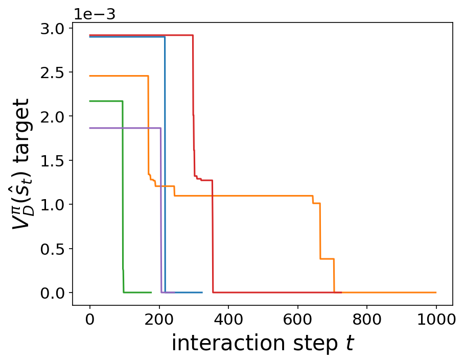
Figure 2: $V_{D}^{\pi}(\hat{s}_{t})$ target of five sampled episodes.

where $L$ denotes Mean Squared Error (MSE), $\hat{y}_{t}$ is the prediction, ${y}_{t}$ is the fitting target and ${w}$ is the penalty weight. To account for the initial step (${t=0}$), we set ${y_{t-1}}$ to sufficiently large, thereby disregarding the weighted term associated with the first step. In essence, the rationale is to penalize any prediction that violates the non-increasing characteristics of the target sequence, thereby leading to an improved fitting quality.

Line search scheduling

Note that in (11), there are two constraints: (a) the trust region and (b) the bound on expected advantages. In practice, due to approximation errors, constraints in (11) might become infeasible. In that case, we perform a recovery update that only enforces the cost advantage $A_{D}^{\pi}$ to decrease starting from early training steps (in first $k_{\mathrm{safe}}$ updates), and starts to enforce reward improvements of $A^{\pi}$ towards the end of training. This is different from (Zhao et al. 2023b), where the reward improvements are enforced at all times. This is because SCPO only guarantees safety (constraint satisfaction) after convergence, while S-3PO prioritizes constraining imaginary safety violation. With our line search scheduling, S-3PO is able to first grasp a safe policy, and then improve the reward performance. In that way, S-3PO achieves zero safety violation both during training and in testing with a worst-case performance degradation guarantee.

Algorithm 1 S-3PO

Input: Initial policy $\pi_{0}\in\Pi_{\theta}$.

for $k=0,1,2,\dots$ do

     for $t=0,1,2,\dots$ do

         Sample nominal action $a^{r}_{t}\sim\pi_{k}(s_{t})$

         Compute and execute $a_{t}=\mathrm{ISSA}(s_{t},a^{r}_{t})$

         Log $\tau\leftarrow\tau\cup\{(s_{t},a_{t},r_{t},s_{t+1},\Delta\phi_{t})\}$

     end for

     $g\leftarrow\left.\nabla_{\theta}\mathbb{E}_{\hat{s},a\sim\tau}\left[A^{\pi}(\hat{s},a)\right]\right\rvert_{\theta=\theta_{k}}$

     $b\leftarrow\left.\nabla_{\theta}\mathbb{E}_{\hat{s},a\sim\tau}\left[A^{\pi}_{D}(\hat{s},a)\right]\right\rvert_{\theta=\theta_{k}}$

     $c\leftarrow\mathcal{J}_{D}(\pi_{k})+2(H+1)\epsilon_{D}^{\pi}\sqrt{\delta/2}$

     $H\leftarrow\left.\nabla^{2}_{\theta}\mathbb{E}_{\hat{s}\sim\tau}[\mathcal{D}_{KL}(\pi\|\pi_{k})[\hat{s}]]\right\rvert_{\theta=\theta_{k}}$

     $\theta^{*}_{k+1}=\mathop{\underset{\theta}{\mathop{\mathbf{argmax}}}}~{}g^{\top}(\theta-\theta_{k})~{}\mathop{\mathbf{s.t.}}$

     $~{}~{}~{}\frac{1}{2}(\theta-\theta_{k})^{\top}H(\theta-\theta_{k})\leq\delta,c+b^{\top}(\theta-\theta_{k})\leq 0$

     Get search direction $\Delta\theta^{*}\leftarrow\theta^{*}_{k+1}-\theta_{k}$

     for $j=0,1,2,\dots$ do $\triangleright$ Line search

         $\theta^{\prime}\leftarrow\theta_{k}+\xi^{j}\Delta\theta^{*}$

         if  $\mathbb{E}_{\hat{s}\sim\tau}[\mathcal{D}_{KL}(\pi_{\theta^{\prime}}\|\pi_{k})[\hat{s}]]\leq\delta$ and

$\mathbb{E}_{\hat{s},a\sim\tau}\left[A^{\pi_{\theta^{\prime}}}_{D}(\hat{s},a)-A^{\pi_{k}}_{D}(\hat{s},a)\right]\leq\mathrm{max}(-c,0)$ and

$(k\leq k_{\mathrm{safe}}~{}\mathrm{or}~{}\mathbb{E}_{\hat{s},a\sim\tau}\left[A^{\pi_{\theta^{\prime}}}(\hat{s},a)\right]\geq\mathbb{E}_{\hat{s},a\sim\tau}\left[A^{\pi_{k}}(\hat{s},a)\right])$ then

              $\theta_{k+1}\leftarrow\theta^{\prime}$ $\triangleright$ Update policy

              break

         end if

     end for

end for

6 Theoretical Results

In this section, We present three theorems, including (i) zero violation exploration (Theorem 1), (ii) state-wise safety guarantee of S-3PO (Theorem 2), and (iii) worst case performance guarantee of S-3PO (Theorem 3). The proofs of the three theorems are summarized in Appendix C, Appendix D and Appendix E, respectively.

Theorem 1 (Zero Training Time Violation).

If the system satisfies Assumption 1, and the safety index design follows the rule described in (12), the implicit safe set algorithm ensures the system is forward invariant in $\mathcal{\bar{S}}\subset\mathcal{S}_{S}$.

Theorem 2 (Safety Guarantee of S-3PO).

If $\pi_{k},\pi_{k+1}$ are related by applying S-3PO and $s_{t}\in\mathcal{\bar{S}}$, then $s_{t+1}=f(s_{t},\pi_{k+1}(s_{t}))\in\mathcal{\bar{S}}$ in expectation.

Theorem 3 (Worst-case Performance Degradation in S-3PO.).

After $k_{safe}$ updates, suppose $\pi_{k},\pi_{k+1}$ are related by S-3PO update rules, with $\epsilon^{\pi_{k+1}}\doteq\mathbf{max}_{\hat{s}}|\mathbb{E}_{a\sim\pi_{k+1}}[A^{\pi_{k}}(\hat{s},a)]|$, then performance return for $\pi_{k+1}$ satisfies

$$\mathcal{J}(\pi_{k+1})-\mathcal{J}(\pi_{k})\geq-\frac{\sqrt{2\delta}\gamma\epsilon^{\pi_{k+1}}}{1-\gamma}.$$

Remark 4.

Theorem 1 shows zero safety violation exploration by proving the system state will never leave $\mathcal{\bar{S}}$ under the safeguard of ISSA. Theorem 2 shows that by satisfying the constraint of (11), the new policy is guaranteed to generate safe action, i.e. $a\in\mathcal{A}_{S}^{D}$, in expectation. Intuitively, Theorem 3 shows that with enough training epochs, the reward performance of S-3PO will not deteriorate too much after each update.

7 Experiments

In our experiments, we aim to answer the following questions: Q1: Does S-3PO achieve zero-violation during the training?
Q2: How does S-3PO without safeguard compare with other state-of-the-art safe RL methods?
Q3: Does S-3PO learn to act without safeguard?
Q4: How does weighted loss trick impact the performance of S-3PO?
Q5: Is “imaginary” cost necessary to achieve zero violation?
Q6: How does S-3PO scale to high dimensional robots?

7.1 Experiments Setup

To answer these questions, we conducted our experiments on the safe reinforcement learning benchmark GUARD (Zhao et al. 2023a) which is based on Mujoco and Gym interface.

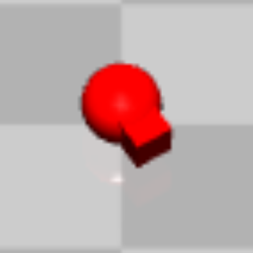
(a) Point

(b) Swimmer

(c) Ant

Figure 3: Robots for benchmark problems in our environment.

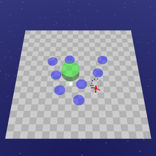
(a) Hazard

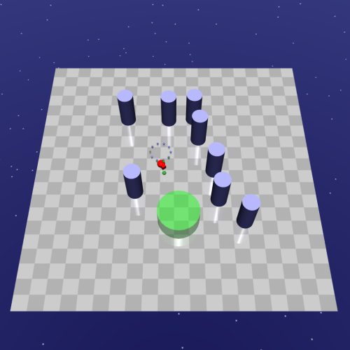
(b) Pillar

Figure 4: Constraints for benchmark problems in our environment.

Environment Setting

We design experimental environments with different task types, constraint types, constraint numbers and constraint sizes. We name these environments as {Task}_{Robot}_{Constraint Number}{Constraint Type}. All of environments are based on Goal where the robot must navigate to a goal.

Our experiments revolve around four distinct robotic entities that can be categorized into two primary types:

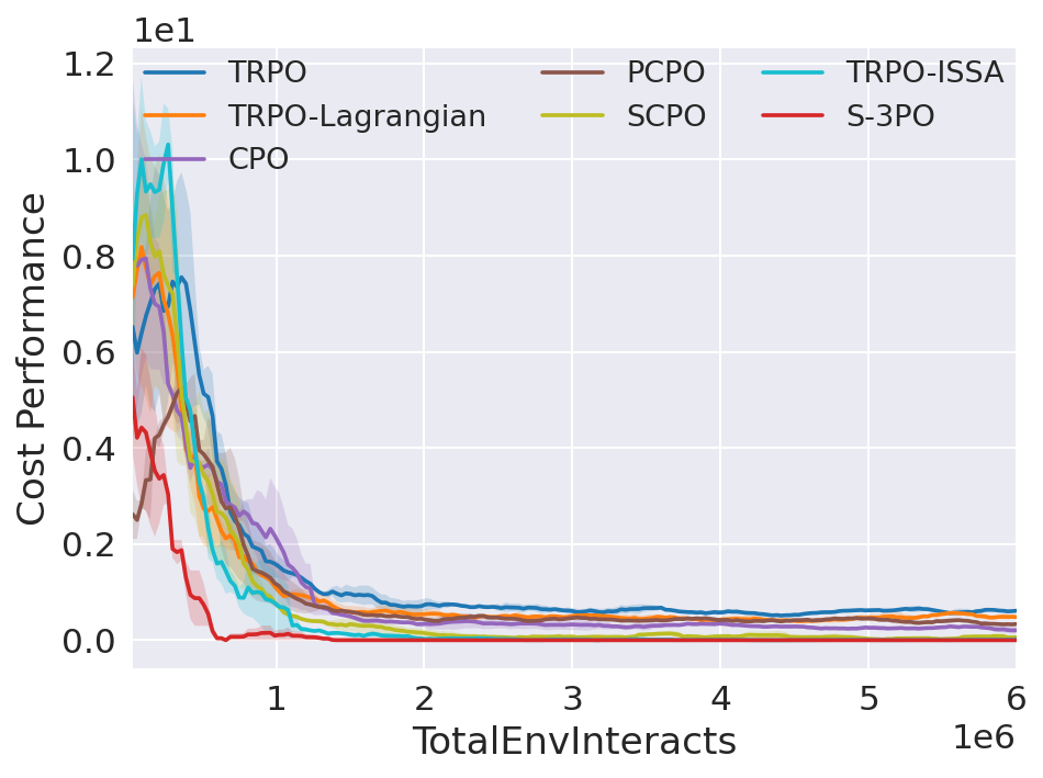
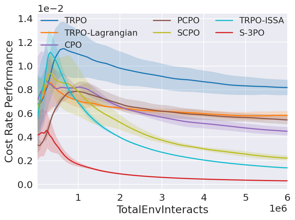
(a) Goal_Point_1Hazard

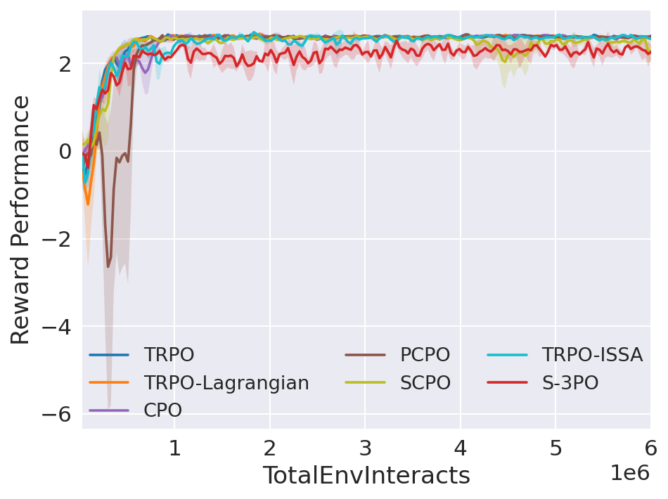
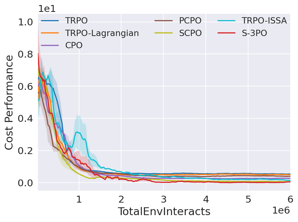
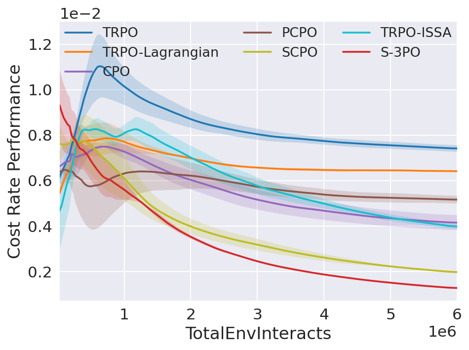
(b) Goal_Point_8Hazard

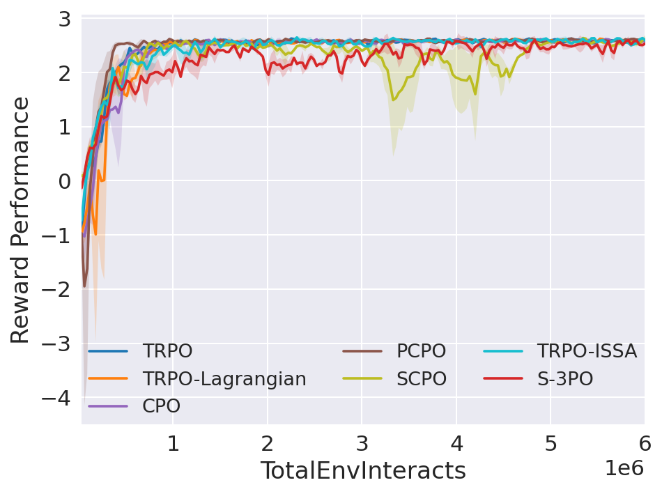
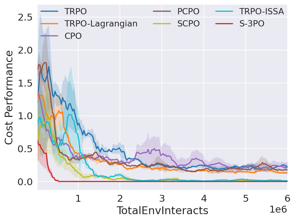
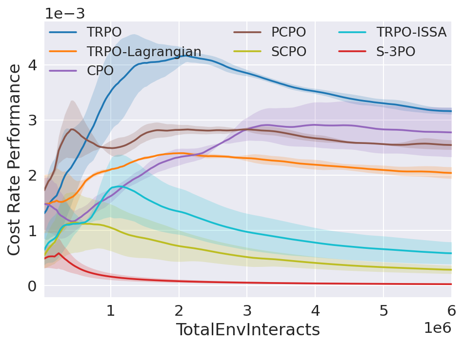
(c) Goal_Point_1Pillar

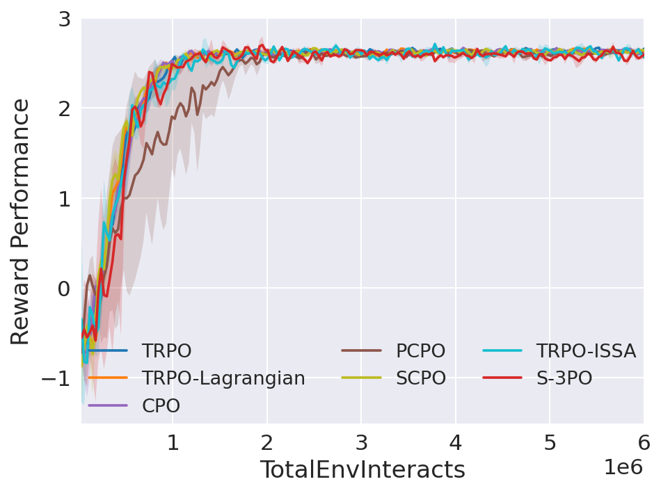
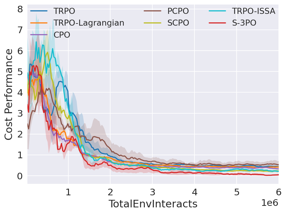
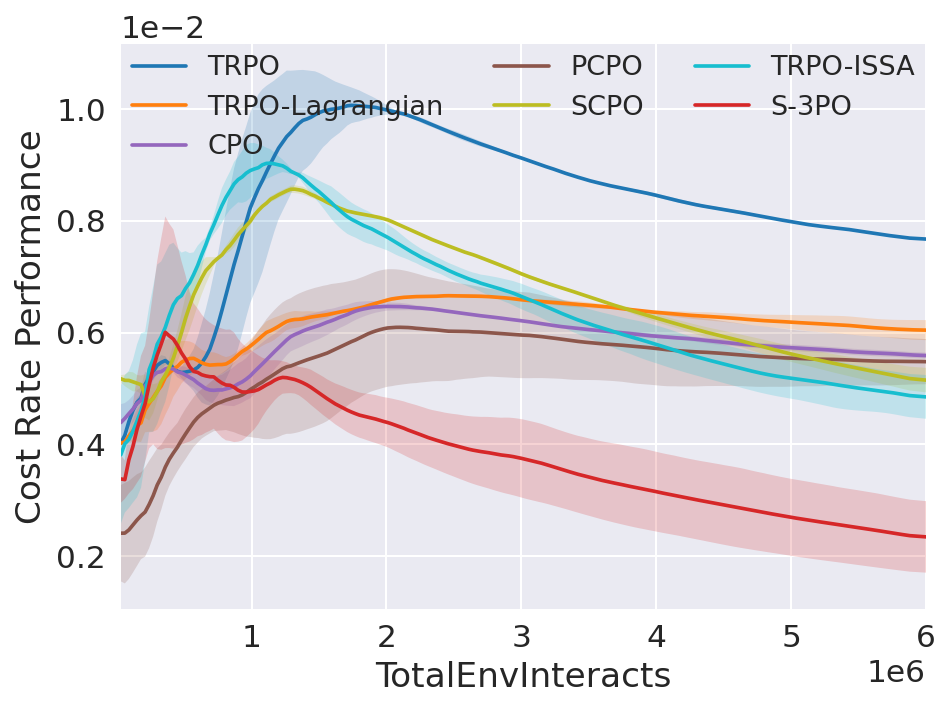
(d) Goal_Swimmer_1Hazard

Figure 6: Results from four representative test suites in low dimensional systems (evaluated without the safeguard).

1. Wheel Robot: this category encompasses robots that use wheels for locomotion, maintaining a continuous and seamless interaction with their surrounding environment. An example is the Point in fig. 3(a) which is designated as $\mathcal{A}\subseteq\mathbb{R}^{2}$.

2. Link Robot: this group includes robots composed of multiple connected links, which interact intermittently with their surroundings through the extremities of these links. Furthermore, the shape of these robots can undergo dynamic changes during these interactions. Specifically, in our environment, we have 1) Swimmer shown in fig. 3(b) as a three-link robot ($\mathcal{A}\subseteq\mathbb{R}^{2}$); 2) Ant shown in fig. 3(c) as a quadrupedal robot ($\mathcal{A}\subseteq\mathbb{R}^{8}$).

Two different types of constraints are considered.

1. Hazard: Dangerous areas shown in fig. 4(a). Hazards are trespassable circles on the ground. The agent is penalized for entering them.

2. Pillar: Fixed obstacles shown in  fig. 4(b). The agent is penalized for hitting them. More details about the experiments are discussed in Section F.1.

Comparison Group

The methods in the comparison group include: (i) unconstrained RL algorithm TRPO (Schulman et al. 2015) and TRPO-ISSA. (ii) end-to-end constrained safe RL algorithms CPO (Achiam et al. 2017), TRPO-Lagrangian (Bohez et al. 2019), PCPO (Yang et al. 2020), SCPO (Zhao et al. 2023b). (iii) We select TRPO as our baseline method since it is state-of-the-art and already has safety-constrained derivatives that can be tested off-the-shelf. For all experiments, the policy $\pi$, the value $(V^{\pi},V_{D}^{\pi})$ are all encoded in feedforward neural networks using two hidden layers of size (64,64) with tanh activations. The full list of parameters of all methods compared can be found in Section F.2.

Evaluation Metrics

For comparison, we evaluate algorithm performance based on (i) reward performance, (ii) average episode cost and (iii) cost rate. More details are provided in Section F.3. We set the limit of cost to 0 for all the safe RL algorithms since we aim to avoid any violation of the constraints.

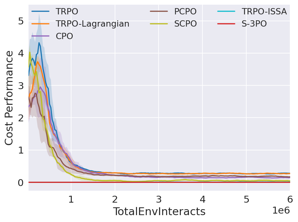
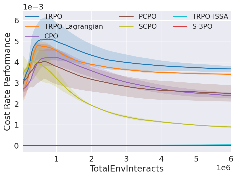
Figure 7: Cost performance of Goal_Point_4Hazard.

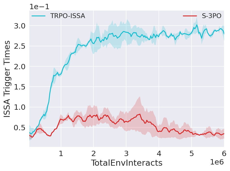
(a) Goal_Point_1Hazard

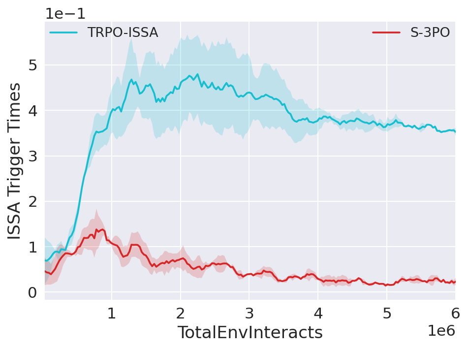
(b) Goal_Point_8Hazard

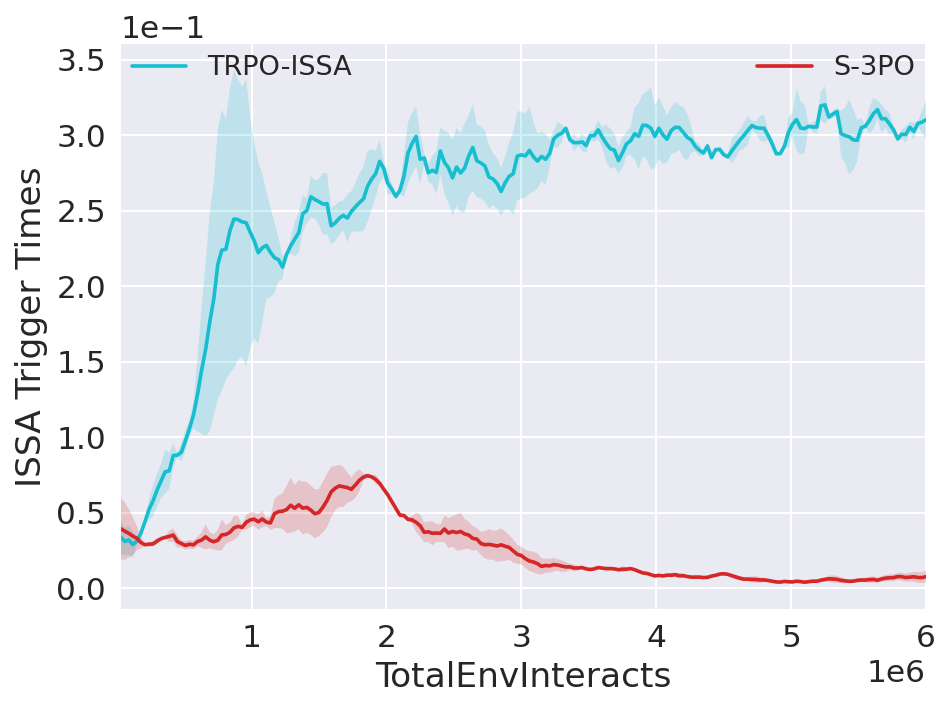
(c) Goal_Point_1Pillar

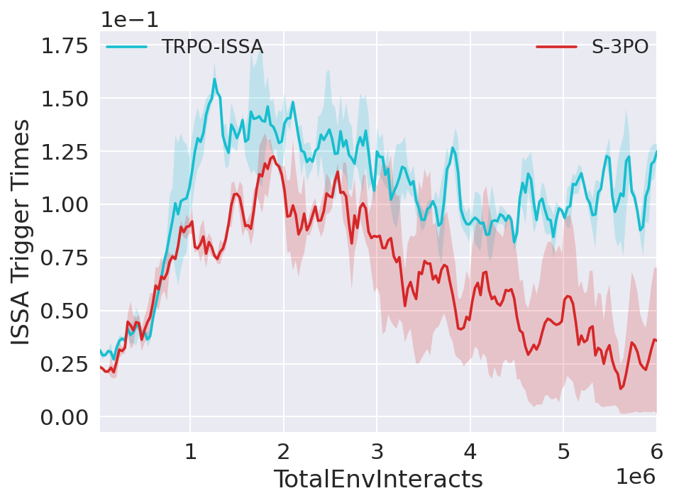
(d) Goal_Swimmer_1Hazard

Figure 9: Triggering frequency of the ISSA-based safeguard in four representative test suites in low dimensional systems.

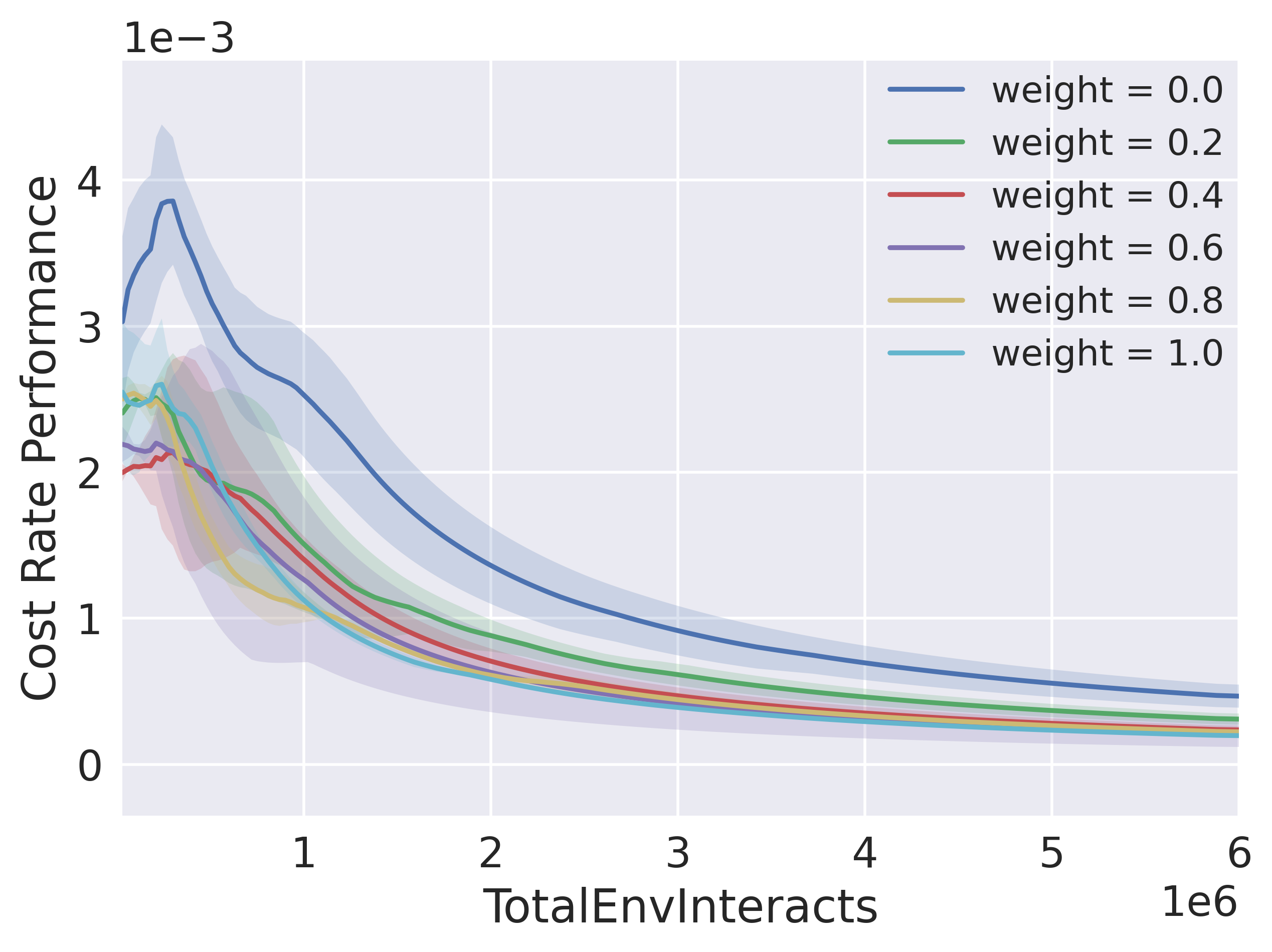
Figure 10: Comparison of cost rate performance with 6 different weights.

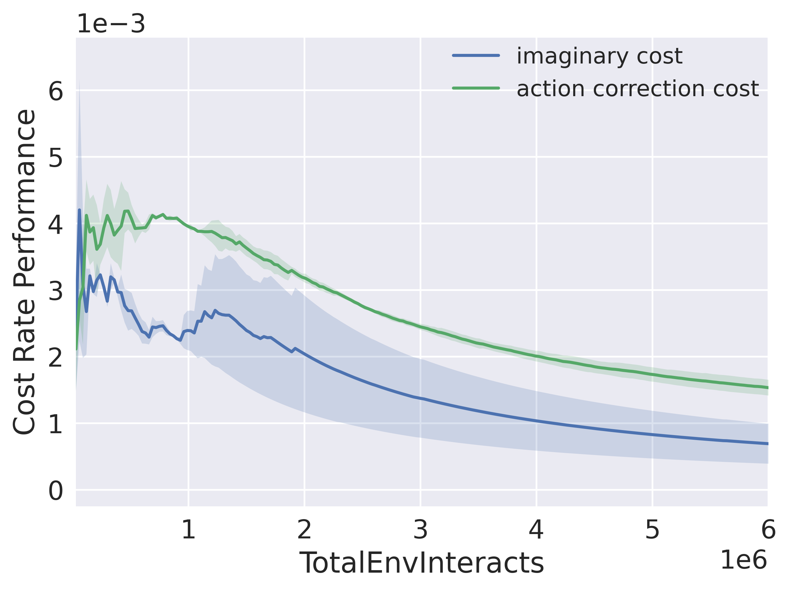
Figure 11: Comparison between “imaginary” cost and action correction cost.

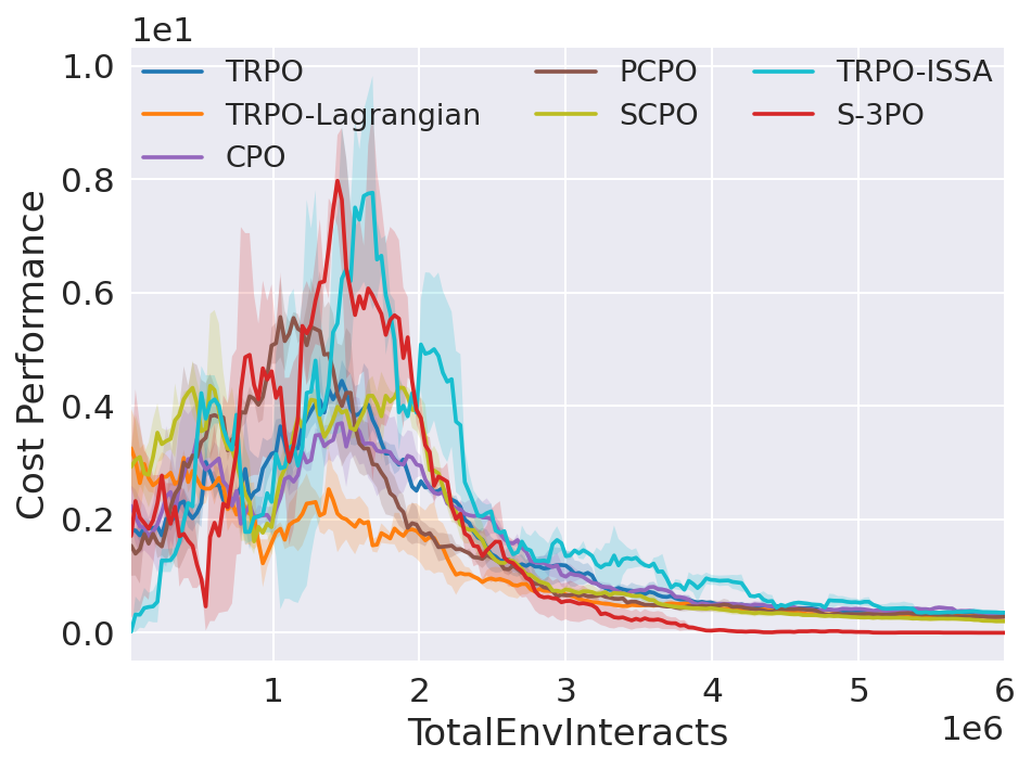
(a) Goal_Ant_1Hazard

(b) Goal_Swimmer_1Hazard

Figure 12: Cost performance of link robots.

7.2 Evaluating S-3PO and Comparison Analysis

Zero Violation during training

The performance results during training are summarized in Figure 7. It is evident that S-3PO algorithm outperforms other baseline methods by achieving zero violations, which is well-aligned with Theorem 1. This advantage is attributed to the adoption of ISSA-based safeguard, which effectively corrects unsafe actions at each step. Moreover, the reward performance continues to improve throughout the learning process and is comparable with state-of-the-art baselines. This unique characteristic of S-3PO enables safe RL with zero safety violation in real-world scenarios, which answers Q1.

State-wise Safety without safety monitor

To evaluate the policy performance of S-3PO without the presence of safeguard, we conduct evaluations at the end of each epoch. During evaluation, the S-3PO policy is evaluated without the safeguard for 10,000 steps. Hence, we can determine if S-3PO effectively learns state-wise safe policy via the guidance of safe set guided cost. The comparative results are shown in Figure 6. When contrasted with baseline safe RL approaches, S-3PO excels without safeguards, achieving (i) near-zero average episode cost and (ii) notably reduced cost rate while maintaining reward performance. The results align well with Theorem 2 and Theorem 3. Importantly, it showcases that through minimizing imaginary safety violation, the policy swiftly learn to act safely, which answers Q2.

Learn to Act without Safeguard

As pointed in 1, the core idea of penalizing imaginary safety violation is to minimize the triggering of the safeguard. To have a better understanding, we visualize in Figure 9 to show the average number of times that the ISSA-based safeguard is triggered per step. Note that TRPO-ISSA is included as a baseline. Figure 9 demonstrates S-3PO significantly reduces the triggering times of the safeguard to stay around 0, which indicates state-wise safe policy is learned and answers Q3.

Ablation on Weighted Loss for Fitting Cost Increment Value Targets

As pointed in Section 5, fitting $V_{D_{i}}(\hat{s}_{t})$ is a critical step towards solving S-3PO, which is challenging due to non-increasing stair shape of the target sequence. To elucidate the necessity of weighted loss for solving this challenge, we evaluate the cost rate of S-3PO under six distinct weight settings (0.0, 0.2, 0.4, 0.6, 0.8, 1.0) on Goal_Point_4Hazard test suite. The results shown in Figure 11 validates that a larger weight (hence higher penalty on predictions that violate the characteristics of value targets) results in better cost rate performance. This ablation study answers Q4.

Necessity of “Imaginary” Cost

To comprehend the significance of the proposed “imaginary” cost, we compare it with another cost that depends on the magnitude of action correction (Chen and Liu 2021). This empirical exploration is conducted in the Goal_Point_4Hazard test suite. As illustrated in Figure 11, it becomes evident that using “imaginary” cost yields superior cost rate performance. This observation implies that the “imaginary” cost can unearth a more profound understanding of the intricate interplay between the robot and its environment, which answers Q5.

Scale S-3PO to High-Dimensional Link Robots

To showcase S-3PO’s scalability and performance with complex, high-dimensional link robots, we conducted additional tests on Goal_Ant_1Hazard featuring 8 dimensional control spaces. The results in Figure 12 underscore S-3PO’s consistent trend of reducing cost to zero. Notably, the relatively lower-dimensional Swimmer robot outperforms other baselines faster than the Ant robot. These insights effectively address Q6 for high-dimensional link robots.

8 Conclusion and Future Prospectus

In this study, we introduce Safe Set Guided State-wise Constrained Policy Optimization (S-3PO), a novel algorithm pioneering state-wise safe optimal policies. This distinction is underlined by the absence of training violations, signifying an error-free learning paradigm. S-3PO employs a safeguard anchored in black-box dynamics to ensure secure exploration. Subsequently, it integrates a novel “imaginary” safety cost to guide the RL agent towards optimal safe policies. S-3PO outperforms existing methods in complex high-dimensional robotics tasks.

Nevertheless, a noteworthy limitation pertains to the potential costliness of acquiring a physical engine-based simulator (black-box dynamics model). A forward-looking perspective entails replacing the black-box dynamics model with a learned surrogate model, factoring in the nuances of errors in learned dynamics. This strategic move holds the promise of obliterating the final barrier impeding the seamless integration of safe RL training into real-world applications.

Appendix A Implicit Safe Set Algorithm Details

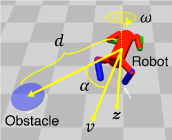
Figure 13: Notations.

Circumstances and Assumptions

In our treatment, both the robot and obstacles assume the form of point-mass circles, confined by finite collision radii. The safety criterion adopts the form $\phi_{0}=\max_{i}{\phi_{0}}_{i}$, with ${\phi_{0}}_{i}=d_{min}-d_{i}$. Here, $d_{i}$ captures the separation between the robot’s center and the $i$-th obstacle, encompassing both static and non-static entities. In this context, we introduce $z$ and $w$ to signify the relative acceleration and relative angular velocity of the robot, respectively, within the obstacle’s frame, as depicted in Figure 13. Importantly, the synthesis of the safety index for 2D collision evasion remains independent of specific dynamic models, but under the following assumption:

Assumption 1 (2D Collision Avoidance).

1) The state space is bounded, and the relative acceleration and angular velocity are bounded and both can achieve zeros, i.e., $w\in[w_{min},w_{max}]$ for $w_{min}\leq 0\leq w_{max}$ and $z\in[z_{min},z_{max}]$ for $z_{min}\leq 0\leq z_{max}$; 2) For all possible values of $z$ and $w$, there always exists a control $a$ to realize such $z$ and $w$; 3) The discrete-time system time step $dt\to 0$; 4) At any given time, there can at most be one obstacle becoming safety critical, such that $\phi-\eta\geq 0$ (Sparse Obstacle Environment).

The bounds in the first assumption will be directly used to synthesize $\phi$. The second assumption enables us to turn the question on whether these exists a feasible control in $\mathcal{A}_{S}^{D}$ to the question on whether there exists $z$ and $w$ to decrease $\phi$. The third assumption ensures that the discrete time approximation error is small. The last assumption enables safety index design rule applicable with multiple moving obstacles.

Safety Index Synthesis

Following the rules in (Liu and Tomizuka 2014), we parameterize the safety index as $\phi=\max_{i}\phi_{i}$, and $\phi_{i}=\sigma+d_{min}^{n}-d_{i}^{n}-k\dot{d}_{i}$, where all $\phi_{i}$ share the same set of tunable parameters $\sigma,n,k,\eta\in\mathbb{R}^{+}$. Our goal is to choose these parameters such that $\mathcal{A}_{S}^{D}(s)$ is always nonempty. By setting $\eta=0$, the parameterization rule of safety index design rule is defined as:

$$\frac{n(\sigma+d_{min}^{n}+kv_{max})^{\frac{n-1}{n}}}{k}\leq\frac{-z_{min}}{v_{max}}$$ (12)

where $v_{max}$ is the maximum relative velocity that the robot can achieve in the obstacle frame. Note that the kinematic constraints $v_{max},z_{min}$ can be obtained by sampling the environment (Zhao, He, and Liu 2021).

Appendix B Additional Algorithms

The main body of AdamBA algorithm is summarized in Algorithm 2, and the main body of ISSA algorithm is summarized in Algorithm 3. The inputs for AdamBA are the approximation error bound ($\epsilon$), learning rate ($\beta$), reference control ($a^{r}$), gradient vector covariance ($\Sigma$), gradient vector number ($n$), reference gradient vector ($\vec{v}^{r}$), safety status of reference control ($S$), and the desired safety status of control solution ($S_{goal}$). The inputs for ISSA are the approximation error bound ($\epsilon$), the learning rate ($\beta$), gradient vector covariance ($\Sigma$), gradient vector number ($n$) and reference unsafe control ($a^{r}$).

Algorithm 2 Adaptive Momentum Boundary Approximation

1:procedure AdamBA($\epsilon,\beta,\Sigma,n,a^{r},\vec{v}^{r},S,S_{goal}$)

2:     Initialize:

3:     if $\vec{v}^{r}$ is empty then

4:         Generate $n$ Gaussian distributed unit gradient vectors $\vec{v}_{i}\sim\mathcal{N}(0,\Sigma)$, $i=1,2,\ldots,n$

5:     else

6:         Initialize one unit gradient vector $\vec{v}_{1}=\frac{\vec{v}^{r}}{\|\vec{v}^{r}\|}$

7:     end if

8:     Approximation:

9:     for $i=1,2,\cdots,n$ do

10:         Initialize the approximated boundary point $P_{i}=a^{r}$, and stage = exponential outreach.

11:         while stage = exponential outreach do

12:              Set $P_{S}\leftarrow P_{i}$ and $P_{NS}\leftarrow P_{i}$

13:              $P_{i}=P_{i}+\vec{v}_{i}\beta$

14:              if $P_{i}$ is out of the control set then

15:                  break

16:              end if

17:              if $P_{i}$ safety status $\neq S$  then

18:                  Set $P_{NS}\leftarrow P_{i}$ , stage $\leftarrow$ exponential decay

19:                  break

20:              end if

21:              $\beta=2\beta$

22:         end while

23:         if stage = exponential decay then

24:              Apply Bisection method to locate boundary point until $\|P_{NS}-P_{S}\|<\epsilon$

25:              Set $P_{i}\leftarrow P_{S}$ if $S_{goal}=S$, $P_{i}\leftarrow P_{NS}$ otherwise

26:         end if

27:     end for

28:     Return Approximated Boundary Set $P$

29:end procedure

Algorithm 3 Implicit Safe Set Algorithm (ISSA)

1:procedure ISSA($\epsilon,\beta,\Sigma,n,a^{r}$)

2:     Phase 1: $\triangleright$ Phase 1

3:     Use AdamBA($\epsilon,\beta,\Sigma,n,a^{r},\emptyset,\textit{UNSAFE},\textit{SAFE}$) to sample a collection $\mathbb{S}$ of safe control on the boundary of $\mathcal{A}_{S}^{D}$.

4:     if $\mathbb{S}=\emptyset$ then

5:         Enter Phase 2

6:     else

7:         For each primitive action $a_{i}\in\mathbb{S}$, compute the deviation $d_{i}=\|a_{i}-a^{r}\|^{2}$

8:         return $\mathop{\mathbf{argmin}}_{a_{i}}d_{i}$

9:     end if

10:     

11:     Phase 2: $\triangleright$ Phase 2

12:     Use grid sampling by iteratively increasing sampling resolution to find an anchor safe control $a^{u}$, s.t. safety status of $a^{u}$ is SAFE.

13:     Use AdamBA($\epsilon,\frac{\|a^{r}-a^{u}\|}{4},\Sigma,1,a^{r},\frac{a^{u}-a^{r}}{\|a^{u}-a^{r}\|},\textit{UNSAFE},\textit{SAFE}$) to search for boundary point $a^{*}$

14:     if $a^{*}$ is not found then

15:         Use AdamBA($\epsilon,\frac{\|a^{r}-a^{u}\|}{4},\Sigma,1,a^{u},\frac{a^{r}-a^{u}}{\|a^{r}-a^{u}\|},\textit{SAFE},\textit{SAFE}$) to search for boundary point ${a^{u}}^{*}$

16:         Return ${a^{u}}^{*}$

17:     else

18:         Return $a^{*}$

19:     end if

20:end procedure

Appendix C Proof of Theorem 1

To prove the Theorem 1 we introduce two important corollaries to show that 1) the set of safe control is always nonempty if we choose a safety index that satisfies the design rule in (12); and 2) the proposed algorithm 3 is guaranteed to find a safe control if there exists one. With these two corollaries, it is then straightforward to prove the Theorem 1.

C.1 Feasibility of the Safety Index for Continuous-Time System

Corollary 1 (Non-emptiness of the set of safe control).

If 1) the dynamic system satisfies the conditions in Assumption 1; and 2) the safety index is designed according to the rule in Appendix A, then the robot system in 2D plane has nonempty set of safe control at any state, i.e., $\mathcal{A}_{S}^{D}(s)\neq\emptyset,\forall s$.

Note that the set of safe control $\mathcal{A}_{S}^{D}(s):=\{a\in\mathcal{A}\mid\phi(f(s,a))\leq\max\{\phi(s)-\eta,0\}\}$ is non-empty if and only if it is non-empty in the following two cases: $\phi(s)-\eta<0$ or $\phi(s)-\eta\geq 0$. In the following discussion, we first show that the safety index design rule guarantees a non-empty set of safe control if there’s only one obstacle when $\phi(s)-\eta\geq 0$ (Lemma 1). Then we show that the set of safe control is non-empty if there’s only one obstacle when $\phi(s)-\eta<0$ (Lemma 2). Finally, we leverage Lemma 1 and Lemma 2 to show $\mathcal{A}_{S}^{D}(s)$ is non-empty if there’re multiple obstacles at any state.

Lemma 1.

If the dynamic system satisfies the conditions in Assumption 1 and there is only one obstacle in the environment, then the safety index design rule in Appendix A ensures that $\mathcal{A}_{S}^{D}(s)\neq\emptyset$ for $x$ such that $\phi(s)-\eta\geq 0$.

Proof.

For $x$ such that $\phi(s)-\eta\geq 0$, the set of safe control becomes

$$\mathcal{A}_{S}^{D}(s)=\{a\in\mathcal{A}\mid\phi(f(s,a))\leq\phi(s)-\eta\}$$ (13)

According to the third condition in Assumption 1, we have $dt\rightarrow 0$. Therefore, the discrete-time approximation error approaches zero, i.e., $\phi(f(s,a))=\phi(s)+dt\cdot\dot{\phi}(s,a)+\Delta$, where $\Delta\rightarrow 0$. Then we can rewrite (13) as:

$$\mathcal{A}_{S}^{D}(s)=\{a\in\mathcal{A}\mid\dot{\phi}\leq-\eta/dt\}$$ (14)

According to the definition of $\phi$, we have $\dot{\phi}=-nd^{n-1}\dot{d}-k\ddot{d}$. We ignored the subscript $i$ since it is assumed that there is only one obstacle. Therefore, the non-emptiness of $\mathcal{A}_{S}^{D}(s)$ in (14) is equivalent to the following condition

$$\forall s\text{ s.t. }\phi(s)\geq\eta,\exists a,\text{s.t. }\ddot{d}\geq\frac{\eta/dt-nd^{n-1}\dot{d}}{k}.$$ (15)

Note that in the 2D problem, $\ddot{d}=-z\cos(\alpha)+v\sin{(\alpha)}w$ and $\dot{d}=-v\cos(\alpha)$. According to Assumption 1, there is a surjection from $a$ to $(z,w)\in W:=\{(z,w)\mid z_{min}\leq z\leq z_{max},w_{min}\leq w\leq w_{max}\}$. Moreover, according to the definition of safety index, $\phi$ for the 2D problem only depends on $\alpha$, $v$, and $d$. Hence condition $\forall s\text{ s.t. }\phi(s)\geq\eta$ can be translated to $\forall(\alpha,v,d)\text{ s.t. }\sigma+d_{min}^{n}-d^{n}-kv\cos(\alpha)\geq\eta$. Denote the later set as

$$\Phi:=\{(\alpha,v,d)\mid\sigma+d_{min}^{n}-d^{n}-kv\cos(\alpha)\geq\eta,v\in[0,v_{max}],d\geq 0,\alpha\in[0,2\pi)\}.$$ (16)

Consequently, condition (6) is equivalent to the following condition

$$\forall(\alpha,v,d)\in\Phi,\exists(z,w)\in W,\text{ s.t. }-z\cos(\alpha)+v\sin(\alpha)w \geq\frac{\eta/dt+nd^{n-1}v\cos(\alpha)}{k}.$$ (17)

According to the safety index design rule, we have $\eta=0$. Then we show (17) holds in different cases.

Case 1: $v=0$. In this case, we can simply choose $z=0$, then the inequality in (17) holds.

Case 2: $v\neq 0$ and $\cos(\alpha)\leq 0$. Note that velocity $v$ is always non-negative. Hence $v>0$. In this case, we just need to choose $z=w=0$, then the inequality in (17) holds, where the LHS becomes zero and the RHS becomes $\frac{nd^{n-1}v\cos(\alpha)}{k}$ which is non-positive.

Case 3: $v\neq 0$ and $\cos(\alpha)>0$. Dividing $v\cos(\alpha)$ on both sides of the inequality and rearranging the inequality, (17) is equivalent to

$$\forall(\alpha,v,d)\in\Phi,\exists(z,w)\in W,\text{ s.t. }-\frac{z}{v}+\tan(\alpha)w-\frac{nd^{n-1}}{k}\geq 0,$$ (18)

and (18) can be verified by showing:

$$\min_{(\alpha,v,d)\in\Phi}\max_{(z,w)\in W}(-\frac{z}{v}+\tan(\alpha)w-\frac{nd^{n-1}}{k})\geq 0.$$ (19)

Now let us expand the LHS of (19):

$$\min_{(\alpha,v,d)\in\Phi}\max_{(z,w)\in W}(-\frac{z}{v}+\tan(\alpha)w-\frac{nd^{n-1}}{k})$$ (20)

$$= \min_{(\alpha,v,d)\in\Phi}(-\frac{z_{min}}{v}+[\tan(\alpha)]_{+}w_{max}+[\tan(\alpha)]_{-}w_{min}-\frac{nd^{n-1}}{k})$$ (21)

$$= \min_{\alpha\in[0,2\pi),v\in(0,v_{max}]}(-\frac{z_{min}}{v}+[\tan(\alpha)]_{+}w_{max}+[\tan(\alpha)]_{-}w_{min}-\frac{n(\sigma+d_{min}^{n}+kv\cos(\alpha))^{\frac{n-1}{n}}}{k})$$ (22)

$$= -\frac{z_{min}}{v_{max}}-\frac{n(\sigma+d_{min}^{n}+kv_{max})^{\frac{n-1}{n}}}{k}.$$ (23)

The first equality eliminates the inner maximization where $[\tan(\alpha)]_{+}:=\max\{\tan(\alpha),0\}$ and $[\tan(\alpha)]_{-}:=\min\{\tan(\alpha),0\}$. The second equality eliminates $d$ according to the constraint in $\Phi$. The third equality is achieved when $\alpha=0$ and $v=v_{max}$. According to the safety index design rule in Appendix A, (23) is greater than or equal to zero. Hence (19) holds, which then implies that the inequality in (17) holds.

The three cases cover all possible situations. Hence (17) always hold and the claim in the lemma is verified. ∎

Lemma 2.

If the dynamic system satisfies the contidions in Assumption 1 and there is only one obstacle in the environment, then the safety index design rule in Appendix A ensures that $\mathcal{A}_{S}^{D}(s)=\mathcal{A}$ for any $s$ that $\phi(s)-\eta<0$.

Proof.

For $s$ such that $\phi(s)-\eta<0$, the set of safe control becomes

$$\mathcal{A}_{S}^{D}(s)=\{a\in\mathcal{A}\mid\phi(f(s,a))\leq 0\}$$ (24)

According to the third assumption in Assumption 1, we have $dt\rightarrow 0$. Therefore, the discrete-time approximation error approaches zero, i.e., $\phi(f(s,a))=\phi(s)+dt\cdot\dot{\phi}(s,a)+\Delta$, where $\Delta\rightarrow 0$. Then we can rewrite (24) as:

$$\mathcal{A}_{S}^{D}(s)=\{a\in\mathcal{A}\mid\dot{\phi}\leq-\phi/dt\}$$ (25)

Note that $\eta=0$ according to the safety index design rule, then $\phi(s)-\eta<0$ implies that $\phi(s)<0$. Hence $-\phi/dt\rightarrow\infty$ since $dt\rightarrow 0$. Then as long as $\dot{\phi}$ is bounded, $\mathcal{A}_{S}^{D}(s)=\mathcal{A}$.

Now we show that $\dot{\phi}$ is bounded. According to the definition of safety index design rule, $\dot{\phi}=-nd^{n-1}\dot{d}-k\ddot{d}$. We ignored the subscript $i$ since it is assumed that there is only one obstacle. According to Assumption 1, we have the state space is bounded, thus both $d$ and $\dot{d}$ are bounded, which implies that $nd^{n-1}\dot{d}$ is bounded. Moreover, we have for all possible values of $z$ and $w$, there always exists a control $a$ to realize such $z$ and $w$ according to Assumption 1, which indicates the mapping from $a$ to $(z,w)$ is surjective. Since $z$ and $w$ are bounded and both can achieve zeros according to Assumption 1, we have $\forall a$, the corresponding $(z,w)$ are bounded. Since $\ddot{d}=-z\cos(\alpha)+v\sin(\alpha)w$, then $\ddot{d}$ is bounded. Hence $\mathcal{A}_{S}^{D}(s)=\mathcal{A}$ any $s$ that $\phi(s)-\eta<0$ and the claim is true. ∎

Proof of Corollary 1.

Proof.

If there is one obstacle, then lemma 1 and lemma 2 have proved that $\mathcal{A}_{S}^{D}(s)\neq\emptyset$ for all $s$. Now we need to consider the case where there are more than one obstacle but the environment is sparse in the sense that at any time step, there is at most one obstacle which is safety critical, i.e. $\phi_{i}\geq 0$. To show nonemptiness of $\mathcal{A}_{S}^{D}(s)$, we consider the following two cases. In the following discussion, we set $\eta=0$ according to the safety index design rule.

Case 1: $\phi(s)=\max_{i}\phi_{i}(s)\geq 0$. Denote $j:=\arg\max_{i}\phi_{i}(s)$. Since there is at most one obstacle that is safety critical, then $\phi_{j}(s)\geq 0$ and $\phi_{k}(s)<0$ for all $k\neq j$.

Denote ${\mathcal{A}_{S}^{D}}_{j}(s):=\{a\in\mathcal{A}\mid\phi_{j}(f(s,a))\leq\phi_{j}(s)\}$. Lemma 1 ensures that ${\mathcal{A}_{S}^{D}}_{j}(s)$ is nonempty. Denote ${\mathcal{A}_{S}^{D}}_{k}(s):=\{a\in\mathcal{A}\mid\phi_{k}(f(s,a))\leq 0\}$ where $k\neq j$. Since $\phi_{k}(s)<0$, lemma 2 ensures that ${\mathcal{A}_{S}^{D}}_{k}(s)=\mathcal{A}$.

Note that the set of safe control can be written as:

$${\mathcal{A}_{S}^{D}}(s) :=\{a\in\mathcal{A}\mid\max_{i}\phi_{i}(f(s,a))\leq\max_{i}\phi_{i}(s)\}$$ (26a)

$$=\{a\in\mathcal{A}\mid\max_{i}\phi_{i}(f(s,a))\leq\phi_{j}(s)\}$$ (26b)

$$=\cap_{i}\{a\in\mathcal{A}\mid\phi_{i}(f(s,a))\leq\phi_{j}(s)\}$$ (26c)

$$={\mathcal{A}_{S}^{D}}_{j}(s)\neq\emptyset$$ (26d)

Note that the last equality is due to the fact that $\{a\in\mathcal{A}\mid\phi_{i}(f(s,a))\leq\phi_{j}(s)\}\supseteq\{a\in\mathcal{A}\mid\phi_{i}(f(s,a))\leq 0\}=\mathcal{A}\supseteq{\mathcal{A}_{S}^{D}}_{j}(s)$ for $i\neq j$.

Case 2: $\phi(s)=\max_{i}\phi_{i}(s)<0$. Therefore, we have $\phi_{i}(s)<0$ for all $i$. According to Lemma 2, $\{a\in\mathcal{A}\mid\phi_{i}(f(s,a))\leq 0\}=\mathcal{A}$. Hence the set of safe control satisfies the following relationship

$${\mathcal{A}_{S}^{D}}(s) :=\{a\in\mathcal{A}\mid\max_{i}\phi_{i}(f(s,a))\leq 0\}$$ (27a)

$$=\cap_{i}\{a\in\mathcal{A}\mid\phi_{i}(f(s,a))\leq 0\}$$ (27b)

$$=\mathcal{A}\neq\emptyset$$ (27c)

In summary, $\mathcal{A}_{S}^{D}(s)\neq\emptyset,\forall s$ and the claim holds. ∎

C.2 Feasibility of ISSA

Corollary 2 (Feasibility of Algorithm 3).

If the set of safe control is non-empty, Algorithm 3 can always find a sub-optimal solution of (6) with a finite number of iterations.

Algorithm 3 executes two phases consecutively where the second phase will be executed if no solution of (6) is returned in the first phase. Hence, Algorithm 3 can always find a sub-optimal solution of (6) (safe control on the boundary of $\mathcal{A}_{S}^{D}$) if the solution of (6) can always be found in phase 2.

Note that Phase 2 first finds an anchor safe control $a^{u}$, then use it with AdamBA (Algorithm 2) to find the solution of (6). In the following discussion, we first show that the safety index design rule guarantees $a^{u}$ can be found with finite iterations (Lemma 3). Then we show that AdamBA will return a solution if it enters the exponential decay phase (Lemma 4). Subsequently, we show that the evoked AdamBA procedures in phase 2 will definitely enter exponential decay phase (Lemma 5). Finally, we provide a upper bound of the computation iterations for Algorithm 3.

Lemma 3 (Existence).

If the synthesized safety index can guarantee a non-empty set of safe control, then we can find an anchor point in phase 2 of Algorithm 3 with finite iterations (line 11 in algorithm 3).

Proof.

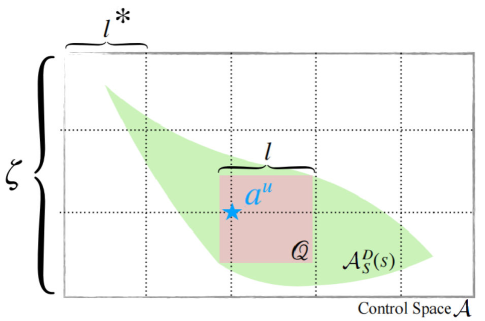
Figure 14: Illustration of the grid sampling to find an anchor control point.

If the synthesized safety index guarantees a non-empty set of safe control $\mathcal{A}^{D}_{S}$, then there exists a hypercube inside of $\mathcal{A}^{D}_{S}$, i.e. $\exists\mathcal{Q}\subset\mathcal{A}_{S}^{D}$, where $\mathcal{Q}$ is a $n_{u}$-dimensional hypercube with the same side length of $l>0$. Denote $\zeta_{[i]}=\max_{j,k}\|a_{[i]}^{j}-a_{[i]}^{k}\|$, where $a_{[i]}$ denotes the $i$-th dimension of control $a$, and $a^{j}\in\mathcal{A}^{D}_{S},a^{k}\in\mathcal{A}^{D}_{S}$.

By directly applying grid sampling in $\mathcal{A}^{D}_{s}$ with sample interval $l^{*}$ at each control dimension, such that $0<l^{*}<l$, the maximum sampling iteration $T^{a}$ for finding an anchor point in phase 2 satisfies the following condition:

$$T^{a}<\prod\limits_{i=1}^{n_{u}}\lceil\frac{\zeta_{[i]}}{l^{*}}\rceil~{},$$ (28)

where $T^{a}$ is a finite number since $l^{*}>0$. Then we have proved that we can find an anchor point in phase 2 of Algorithm 3 with finite iteration (i.e., finite sampling time). The grid sampling to find an anchor control point is illustrated in Figure 14.

∎

Lemma 4 (Convergence).

If AdamBA enters the exponential decay phase, then it can always return a boundary point approximation (with desired safety status) where the approximation error is upper bounded by $\epsilon$.

Proof.

According to Algorithm 2, exponential decay phase applies Bisection method to locate the boundary point $P_{b}$ until $\|P_{NS}-P_{S}\|<\epsilon$. Denote the returned approximated boundary point as $P_{return}$, according to line 25, $P_{return}$ is either $P_{NS}$ or $P_{S}$, thus the approximation error satisfies:

$$\|P_{return}-P_{b}\| \leq\max\{\|P_{NS}-P_{b}\|,\|P_{S}-P_{b}\|\}$$ (29)

$$\leq\|P_{NS}-P_{S}\|$$

$$<\epsilon.$$

∎

Lemma 5 (Feasibility).

If we enter the phase 2 of Algorithm 3 with an anchor safe control being sampled, we can always find a local optimal solution of (6).

Proof.

According to line 13-15, after an anchor safe control is being sampled, phase 2 of Algorithm 3 will evoke at most two AdamBA processes. Hence, Lemma 5 can be proved by showing one of the two AdamBA will return a local optimal solution for (6). Next we show Lemma 5 holds in two cases.

Case 1:

line 13 of Algorithm 3 finds a solution.

In this case, the first AdamBA process finds a safe control $a^{u}$ solution (the return of AdamBA is a set, whereas the set here has at most one element). According to Algorithm 2, a solution will be returned only if AdamBA enters exponential decay stage. Hence, according to Lemma 4, $a^{u}$ is close to the boundary of the set of safe control with approximation error upper bounded by $\epsilon$.

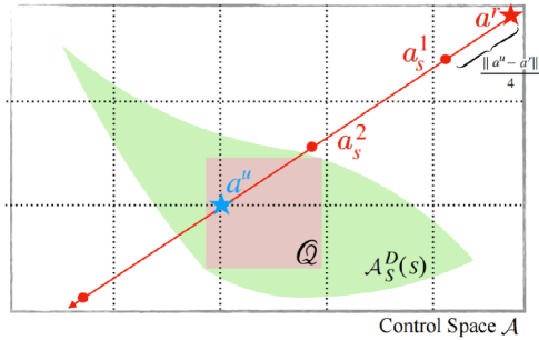
Figure 15: Illustration of the case when it is unable to find $u^{*}$.

Case 2:

line 13 of Algorithm 3 fails to find a solution.

In this case, the second AdamBA process is evoked (line 15 of Algorithm 3). Since no solution is returned from the first AdamBA process (13 of Algorithm 3), where we start from $a^{r}$ and exponentially outreach along the direction $\vec{v}_{a}=\frac{a^{u}-a^{r}}{||a^{u}-a^{r}||}$, then all the searched control point along $\vec{v}_{a}$ is UNSAFE.

Specifically, we summarize the aforementioned scenario in Figure 15, the searched control points are represented as red dots along $\vec{v}_{a}$ (red arrow direction). Note that the exponential outreach starts with step size $\beta=\frac{\|a^{u}-a^{r}\|}{4}$, indicating two points $\{a_{s}^{1}$, $a_{s}^{2}\}$ are sampled between $a^{r}$ and $a^{u}$ such that

$$\begin{cases}a_{s}^{1}=a^{r}+\frac{\|a^{u}-a^{r}\|}{4}\vec{v}_{a}=\frac{3a^{r}}{4}+\frac{a^{u}}{4}\\ a_{s}^{2}=a^{r}+\frac{3\|a^{u}-a^{r}\|}{4}\vec{v}_{a}=\frac{a^{r}}{4}+\frac{3a^{u}}{4}\end{cases}$$ (30)

where the safety statuses of both $a_{s}^{1}$ and $a_{s}^{2}$ are UNSAFE.

During the second AdamBA process (line 15 of Algorithm 3), we start from $a^{u}$ and exponentially outreach along the direction $\vec{v}_{r}=\frac{a^{r}-a^{u}}{||a^{r}-a^{u}||}$ with initial step size $\beta=\frac{\|a^{r}-a^{u}\|}{4}$. Hence, denote $\bar{a}_{s}^{1}$ as the first sample point along $\vec{v}_{r}$, and $\bar{a}_{s}^{1}$ satisfies

$$\bar{a}_{s}^{1}=a^{u}+\frac{\|a^{r}-a^{u}\|}{4}\vec{v}_{r}=\frac{a^{r}}{4}+\frac{3a^{u}}{4},$$ (31)

which indicates $\bar{a}_{s}^{1}=a_{s}^{2}$, and the safety status of $\bar{a}_{s}^{1}$ is UNSAFE. Since the safe status of $a^{u}$ is SAFE and a UNSAFE point can be sampled during the exponential outreach stage, the second AdamBA process (line 15 of Algorithm 3) will enter exponential decay stage. Therefore, according to Lemma 4, ${a^{u}}^{*}$ will always be returned and ${a^{u}}^{*}$ is close to the boundary of the set of safe control with approximation error upper bounded by $\epsilon$.

The two cases cover all possible situations. Hence, after an anchor safe control $a^{u}$ is sampled, phase 2 of Algorithm 3 can always find a local optima of (6).

∎

Proof of Corollary 2.

Proof.

According to Lemma 3 and Lemma 5, Algorithm 3 is able to find local optimal solution of (6). Next, we will prove Algorithm 3 can be finished within finite iterations.

According to Algorithm 3, ISSA include (i) one procedure to find anchor safe control $a_{a}$, and (ii) at most three AdamBA procedures. Firstly, based on Lemma 3, $a_{a}$ can be found within finite iterations. Secondly, each AdamBA procedure can be finished within finite iterations due to:

• exponential outreach can be finished within finite iterations since the control space is bounded.

• exponential decay can be finished within finite iterations since Bisection method will exit within finite iterations.

Therefore, ISSA can be finished within finite iterations.

∎

C.3 Proof of Theorem 1

Before we prove Theorem 1, we first define set $\mathcal{S}_{S}^{D}:=\{s|\phi(s)\leq 0\}$, and we start with a preliminary result regarding $\mathcal{S}_{S}^{D}$ that is useful for proving the main theorem:

Lemma 6 (Forward Invariance of $\mathcal{S}_{S}^{D}$).

If the control system satisfies Assumption 1, and the safety index design follows the rule described Appendix A, the implicit safe set algorithm guarantees the forward invariance to the set $\mathcal{S}_{S}^{D}$.

Proof.

If the control system satisfies the assumptions in Assumption 1, and the safety index design follows the rule described Appendix A, then we can ensure the system has nonempty set of safe control at any state by Corollary 1. By Corollary 2, the implicit safe set algorithm can always find local optima solution of (6). The local optima solution always satisfies the constraint $\phi(f(s_{t},a_{t}))\leq\max\{\phi(s_{t})-\eta,0\}$, which indicates that 1) if $\phi(s_{t_{0}})\leq 0$, then $\phi(s_{t})\leq 0,\forall t\geq t_{0}$. Note that $\phi(s)\leq 0$ demonstrates that $s\in\mathcal{S}_{S}^{D}$. ∎

Proof the Theorem 1

Proof.

Leveraging Lemma 6, we then proceed to prove that the forward invariance to the set $\mathcal{S}_{S}^{D}$ guarantees the forward invariance to the set $\mathcal{\bar{S}}\subseteq\mathcal{S}_{S}$ which $\mathcal{\bar{S}}=\mathcal{S}_{S}\cap\mathcal{S}_{S}^{D}$. Depending on the relationship between $\mathcal{S}_{S}^{D}$ and $\mathcal{S}_{S}$, there are two cases in the proof which we will discuss below.

Case 1: $\mathcal{S}_{S}^{D}=\{s|\phi(s)\leq 0\}$ is a subset of $\mathcal{S}_{S}=\{s|\phi_{0}(s)\leq 0\}$.

In this case, $\mathcal{\bar{S}}=\mathcal{S}_{S}^{D}$. According to Lemma 6, If the control system satisfies the assumptions in Assumption 1, and the safety index design follows the rule described Appendix A, the implicit safe set algorithm guarantees the forward invariance to the set $\mathcal{S}_{S}^{D}$ and hence $\mathcal{\bar{S}}$.

Case 2: $\mathcal{S}_{S}^{D}=\{s|\phi(s)\leq 0\}$ is NOT a subset of $\mathcal{S}_{S}=\{s|\phi_{0}(s)\leq 0\}$.

In this case, if $s_{t}\in\mathcal{\bar{S}}$, we have $\phi_{0}(s_{t})=\max_{i}{\phi_{0}}_{i}(s_{t})\leq 0$, which indicates $\forall i,{\phi_{0}}_{i}\leq 0$.

Firstly, we consider the case where ${\phi_{0}}_{i}(s_{t})<0$. Note that ${\phi_{0}}_{i}(s_{t+1})={\phi_{0}}_{i}(s_{t})+\dot{\phi_{0}}_{i}(s_{t})dt+\frac{\ddot{\phi_{0}}_{i}(s_{t})dt^{2}}{2!}+\cdots$, since the state space and control space are both bounded, and $dt\rightarrow 0$ according to Assumption 1, we have ${\phi_{0}}_{i}(s_{t+1})\rightarrow{\phi_{0}}_{i}(s_{t})\leq 0$.

Secondly, we consider the case where ${\phi_{0}}_{i}(s_{t})=0$. Since $s_{t}\in\mathcal{\bar{S}}$, we have $\max_{i}\phi_{i}(s_{t})\leq 0$, which indicates $\forall i,\sigma+d_{min}^{n}-d_{i}^{n}-k\dot{d}_{i}\leq 0$. Since ${\phi_{0}}_{i}(s_{t})=0$, we also have $d_{i}=d_{min}$. Therefore, the following condition holds:

$$\sigma-k\dot{d}_{i} \leq 0$$ (32)

$$\dot{d}_{i} \geq\frac{\sigma}{k}$$

According to the safety index design rule, we have $k,\sigma\in\mathbb{R}^{+}$, which indicates $\dot{d}_{i}>0$. Therefore, we have ${\phi_{0}}_{i}(s_{t+1})<0$.

Summarizing the above two cases, we have shown that if ${\phi_{0}}_{i}(s_{t})\leq 0$ then ${\phi_{0}}_{i}(s_{t+1})\leq 0$, which indicates if $\forall i,{\phi_{0}}_{i}(s_{t})\leq 0$ then $\forall i,{\phi_{0}}_{i}(s_{t+1})\leq 0$. Note that $\forall i,{\phi_{0}}_{i}(s_{t+1})\leq 0$ indicates that $\phi_{0}(s_{t+1})=\max_{i}{\phi_{0}}_{i}(s_{t+1})\leq 0$. Therefore, we have that if $s_{t}\in\mathcal{\bar{S}}$ then $s_{t+1}\in\mathcal{S}_{S}$. Thus, we also have $s_{t+1}\in\mathcal{\bar{S}}$ by Lemma 6. By induction, we have if $s_{t_{0}}\in\mathcal{\bar{S}}$, $s_{t}\in\mathcal{\bar{S}},\forall t>t_{0}$.

In summary, by discussing the two cases of whether $\mathcal{S}_{S}^{D}$ is the subset of $\mathcal{S}_{S}$, we have proven that if the control system satisfies the assumptions in Assumption 1, and the safety index design follows the rule described in Appendix A, the implicit safe set algorithm guarantees the forward invariance to the set $\mathcal{\bar{S}}\subseteq\mathcal{S}_{S}$. Thus, if the initial state is safe, then the following state will always stay in $\mathcal{\bar{S}}$ which means ISSA can ensure the safety during training.

∎

Appendix D Proof of Theorem 2

Mathematically, S-3PO requires the policy update at each iteration is bounded within a trust region, and updates policy via solving following optimization:

$$\pi_{k+1}=\mathop{\underset{\pi\in\Pi_{\theta}}{\mathop{\mathbf{argmax}}}}\underset{\begin{subarray}{c}\hat{s}\sim d^{\pi_{k}}\\ a\sim\pi\end{subarray}}{\mathbb{E}}[A^{\pi_{k}}(\hat{s},a)]$$ (33)

$$~{}~{}~{}~{}~{}\mathop{\mathbf{s.t.}}~{}~{}\mathbb{E}_{\hat{s}\sim\bar{d}^{\pi_{k}}}[\mathcal{D}_{KL}(\pi\|\pi_{k})[\hat{s}]]\leq\delta,$$

$$~{}~{}~{}~{}~{}~{}~{}~{}~{}~{}~{}~{}\mathcal{J}_{D}(\pi_{k})+\underset{\begin{subarray}{c}\hat{s}\sim\bar{d}^{\pi_{k}}\\ a\sim{\pi}\end{subarray}}{\mathbb{E}}\Bigg{[}A^{\pi_{k}}_{D}(\hat{s},a)\Bigg{]}+2(H+1)\epsilon_{D}^{\pi}\sqrt{\frac{1}{2}\delta}\leq 0$$

where $\mathcal{D}_{KL}(\pi^{\prime}\|\pi)[\hat{s}]$ is KL divergence between two policy $(\pi^{\prime},\pi)$ at state $\hat{s}$, the set $\{\pi\in\Pi_{\theta}~{}:~{}\mathbb{E}_{\hat{s}\sim\bar{d}^{\pi_{k}}}[\mathcal{D}_{KL}(\pi\|\pi_{k})[\hat{s}]]\leq\delta\}$ is called trust region, $d^{\pi_{k}}\doteq(1-\gamma)\sum_{t=0}^{H}\gamma^{t}P(\hat{s}_{t}=\hat{s}|{\pi_{k}})$, $\bar{d}^{\pi_{k}}\doteq\sum_{t=0}^{H}P(\hat{s}_{t}=\hat{s}|{\pi_{k}})$, and $\epsilon^{{\pi}}_{D}\doteq\mathbf{max}_{\hat{s}}|\mathbb{E}_{a\sim{\pi}}[A^{\pi_{k}}_{D}(\hat{s},a)]|$. In practice, if ISSA is triggered, we take $D(\hat{s}_{t},a_{t},\hat{s}_{t+1})=max\{(\phi(f(\hat{s}_{t},a_{t}^{r}))-\phi(f(\hat{s}_{t},a_{t})))-M,0\}=max\{\Delta\phi_{t},0\}$. Otherwise we take $D(\hat{s}_{t},a_{t},\hat{s}_{t+1})=0$ directly.

D.1 Preliminaries

$\dot{d}^{\pi}$ we used is defined as

$$\dot{d}^{\pi}(\hat{s})=\sum\limits_{t=0}^{H}\gamma^{t}P(\hat{s}_{t}=\hat{s}|\pi).$$ (34)

which has a little difference with $d^{\pi}$ and is used to ensure the continuity of function we used for proof later. Then it allows us to express the expected discounted total reward or cost compactly as:

$$\mathcal{J}_{g}(\pi)=\underset{\begin{subarray}{c}\hat{s}\sim\dot{d}^{\pi}\\ a\sim{\pi}\\ \hat{s}^{\prime}\sim P\end{subarray}}{\operatorname{E}}\left[g(\hat{s},a,\hat{s}^{\prime})\right],$$ (35)

where by $a\sim\pi$, we mean $a\sim\pi(\cdot|\hat{s})$, and by $\hat{s}^{\prime}\sim P$,we mean $\hat{s}^{\prime}\sim P(\cdot|\hat{s},a)$. $g(\hat{s},a,\hat{s}^{\prime})$ represents the cost or reward function. We drop the explicit notation for the sake of reducing clutter, but it should be clear from context that $a$ and $\hat{s}^{\prime}$ depend on $\hat{s}$.

Define $P(\hat{s}^{\prime}|\hat{s},a)$ is the probability of transitioning to state $\hat{s}^{\prime}$ given that the previous state was $\hat{s}$ and the agent took action $a$ at state $\hat{s}$, and $\hat{\mu}:\mathcal{\hat{\mathcal{S}}}\mapsto[0,1]$ is the initial augmented state distribution. Let $p_{\pi}^{t}\in\mathbb{R}^{|\hat{\mathcal{S}}|}$ denote the vector with components $p_{\pi}^{t}(\hat{s})=P(\hat{s}_{t}=\hat{s}|\pi)$, and let $P_{\pi}\in\mathbb{R}^{|\hat{\mathcal{S}}|\times|\hat{\mathcal{S}}|}$ denote the transition matrix with components $P_{\pi}(\hat{s}^{\prime}|\hat{s})=\int P(\hat{s}^{\prime}|\hat{s},a)\pi(a|\hat{s})da$; then $p_{\pi}^{t}=P_{\pi}p_{\pi}^{t-1}=P_{\pi}^{t}\hat{\mu}$ and

$$\dot{d}^{\pi} =\sum\limits_{t=0}^{H}(\gamma P_{\pi})^{t}\hat{\mu}$$ (36)

$$=(I-(\gamma P_{\pi})^{H+1})(I-\gamma P_{\pi})^{-1}\hat{\mu}$$

$$=(I-\gamma P_{\pi})^{-1}\hat{\mu}$$

Noticing that the finite MDP ends up at step $H$, thus $(P_{\pi})^{H+1}$ should be set to zero matrix.

This formulation helps us easily obtain the following lemma.

Lemma 7.

For any function $f:\hat{\mathcal{S}}\mapsto\mathbb{R}$ and any policy $\pi$,

$$\underset{\hat{s}\sim\hat{\mu}}{\operatorname{E}}[f(\hat{s})]+\underset{\begin{subarray}{c}\hat{s}\sim\dot{d}^{\pi}\\ a\sim{\pi}\\ \hat{s}^{\prime}\sim P\end{subarray}}{\operatorname{E}}[\gamma f(\hat{s}^{\prime})]-\underset{\hat{s}\sim\dot{d}^{\pi}}{\operatorname{E}}[f(\hat{s})]=0.$$ (37)

Proof.

Multiply both sides of (36) by $(I-\gamma P_{\pi})$ and take the inner product with the vector $f\in\mathbb{R}^{|\hat{\mathcal{S}}|}$. ∎

Combining Lemma 7 with (35), we obtain the following, for any function $f$ and any policy $\pi$:

$$\mathcal{J}_{g}(\pi)=\underset{\hat{s}\sim\hat{\mu}}{\operatorname{E}}\left[f(\hat{s})\right]+\underset{\begin{subarray}{c}\hat{s}\sim\dot{d}^{\pi}\\ a\sim\pi\\ \hat{s}^{\prime}\sim P\end{subarray}}{\operatorname{E}}\left[g(\hat{s},a,\hat{s}^{\prime})+\gamma f(\hat{s}^{\prime})-f(\hat{s})\right]$$ (38)

Lemma 8.

For any function $f\mapsto\mathbb{R}$ and any policies $\pi^{\prime}$ and $\pi$, define

$$L_{\pi,f}(\pi^{\prime})\doteq\underset{\begin{subarray}{c}\hat{s}\sim\dot{d}^{\pi}\\ a\sim\pi\\ \hat{s}^{\prime}\sim P\end{subarray}}{\operatorname{E}}\left[\left(\dfrac{\pi^{\prime}(a|\hat{s})}{\pi(a|\hat{s})}-1\right)(g(\hat{s},a,\hat{s}^{\prime})+\gamma f(\hat{s}^{\prime})-f(\hat{s}))\right],$$ (39)

and $\epsilon_{f}^{\pi\prime}\doteq\max_{\hat{s}}|\mathrm{E}_{a\sim\pi^{\prime},\hat{s}^{\prime}\sim P}[g(\hat{s},a,\hat{s}^{\prime})+\gamma f(\hat{s}^{\prime})-f(\hat{s})]|.$ Then the following bounds hold:

$$\mathcal{J}_{g}(\pi^{\prime})-\mathcal{J}_{g}(\pi)\geq L_{\pi,f}(\pi^{\prime})-\epsilon_{f}^{\pi^{\prime}}\left\|\dot{d}^{\pi^{\prime}}-\dot{d}^{\pi}\right\|_{1},$$ (40)

$$\mathcal{J}_{g}(\pi^{\prime})-\mathcal{J}_{g}(\pi)\leq L_{\pi,f}(\pi^{\prime})+\epsilon_{f}^{\pi^{\prime}}\left\|\dot{d}^{\pi^{\prime}}-\dot{d}^{\pi}\right\|_{1},$$ (41)

where $D_{TV}$ is the total variational divergence. Furthermore, the bounds are tight(when $\pi^{\prime}$ = $\pi$, the LHS and RHS are identically zero).

Proof.

First, for notational convenience, let $\delta_{f}(\hat{s},a,\hat{s}^{\prime})\doteq g(\hat{s},a,\hat{s}^{\prime})+\gamma f(\hat{s}^{\prime})-f(\hat{s})$. By (38), we obtain the identity

$$\mathcal{J}_{g}(\pi^{\prime})-\mathcal{J}_{g}(\pi)=\underset{\begin{subarray}{c}\hat{s}\sim\dot{d}^{\pi^{\prime}}\\ a\sim{\pi^{\prime}}\\ \hat{s}^{\prime}\sim P\end{subarray}}{E}[\delta_{f}(\hat{s},a,\hat{s}^{\prime})]-\underset{\begin{subarray}{c}\hat{s}\sim\dot{d}^{\pi}\\ a\sim\pi\\ \hat{s}^{\prime}\sim P\end{subarray}}{E}[\delta_{f}(\hat{s},a,\hat{s}^{\prime})]$$ (42)

Now, we restrict our attention to the first term in (42). Let $\dagger{\delta}_{f}^{\pi^{\prime}}\in\mathbb{R}^{|\hat{\mathcal{S}}|}$ denote the vector of components, where $\dagger{\delta}_{f}^{\pi^{\prime}}(\hat{s})=\mathbb{E}_{a\sim\pi^{\prime},\hat{s}^{\prime}\sim P}[\delta_{f}(\hat{s},a,\hat{s}^{\prime})|\hat{s}]$. Observe that

$$\underset{\begin{subarray}{c}\hat{s}\sim\dot{d}^{\pi^{\prime}}\\ a\sim{\pi^{\prime}}\\ \hat{s}^{\prime}\sim P\end{subarray}}{\operatorname{E}}[\delta_{f}(\hat{s},a,\hat{s}^{\prime})] =\left\langle\dot{d}^{\pi^{\prime}},\dagger{\delta}_{f}^{\pi^{\prime}}\right\rangle$$

$$=\left\langle\dot{d}^{\pi},\dagger{\delta}_{f}^{\pi^{\prime}}\right\rangle+\left\langle\dot{d}^{\pi^{\prime}}-\dot{d}^{\pi},\dagger{\delta}_{f}^{\pi^{\prime}}\right\rangle$$

With the Hölder’s inequality; for any $p,q\in[1,\infty]$ such that $\dfrac{1}{p}+\dfrac{1}{q}=1$, we have

$$\left\langle\dot{d}^{\pi},\dagger{\delta}_{f}^{\pi^{\prime}}\right\rangle+\left\|\dot{d}^{\pi^{\prime}}-\dot{d}^{\pi}\right\|_{p}\left\|\dagger{\delta}_{f}^{\pi^{\prime}}\right\|_{q}\geq\underset{\begin{subarray}{c}\hat{s}\sim\dot{d}^{\pi^{\prime}}\\ a\sim{\pi^{\prime}}\\ \hat{s}^{\prime}\sim P\end{subarray}}{\operatorname{E}}[\delta_{f}(\hat{s},a,\hat{s}^{\prime})]\geq\left\langle\dot{d}^{\pi},\dagger{\delta}_{f}^{\pi^{\prime}}\right\rangle-\left\|d^{\pi^{\prime}}-\dot{d}^{\pi}\right\|_{p}\left\|\dagger{\delta}_{f}^{\pi^{\prime}}\right\|_{q}$$ (43)

We choose $p=1$ and $q=\infty$; With $\left\|\dagger{\delta}_{f}^{\pi^{\prime}}\right\|_{\infty}=\epsilon_{f}^{\pi^{\prime}}$, and by the importance sampling identity, we have

$$\left\langle\dot{d}^{\pi},\dagger{\delta}_{f}^{\pi^{\prime}}\right\rangle =\underset{\begin{subarray}{c}\hat{s}\sim\dot{d}^{\pi}\\ a\sim{\pi^{\prime}}\\ \hat{s}^{\prime}\sim P\end{subarray}}{\operatorname{E}}[\delta_{f}(\hat{s},a,\hat{s}^{\prime})]$$ (44)

$$=\underset{\begin{subarray}{c}\hat{s}\sim\dot{d}^{\pi}\\ a\sim{\pi}\\ \hat{s}^{\prime}\sim P\end{subarray}}{\operatorname{E}}[\left(\frac{\pi^{\prime}(a|\hat{s})}{\pi(a|\hat{s})}\right)\delta_{f}(\hat{s},a,\hat{s}^{\prime})]$$

After bringing (44), $\left\|\dagger{\delta}_{f}^{\pi^{\prime}}\right\|_{\infty}$ into (43), then substract $\underset{\begin{subarray}{c}\hat{s}\sim\dot{d}^{\pi}\\ a\sim\pi\\ \hat{s}^{\prime}\sim P\end{subarray}}{E}[\delta_{f}(\hat{s},a,\hat{s}^{\prime})]$, the bounds are obtained. The lower bound leads to (40), and the upper bound leads to (41). ∎

Lemma 9.

The divergence between discounted future state visitation distributions, $||\dot{d}^{\pi^{\prime}}-\dot{d}^{\pi}||_{1}$, is bounded by an average divergence of the policies $\pi^{\prime}$ and $\pi$:

$$\|\dot{d}^{\pi^{\prime}}-\dot{d}^{\pi}\|_{1}\leq 2\sum_{t=0}^{H}\gamma^{t+1}\underset{\hat{s}\sim\dot{d}^{\pi}}{\operatorname{E}}\left[D_{TV}(\pi^{\prime}||\pi)[\hat{s}]\right],$$ (45)

where $D_{TV}(\pi^{\prime}||\pi)[\hat{s}]=\dfrac{1}{2}\sum_{a}|\pi^{\prime}(a|\hat{s})-\pi(a|\hat{s})|.$

Proof.

Firstly, we introduce an identity for the vector difference of the discounted future state visitation distributions on two different policies, $\pi^{\prime}$ and $\pi$. Define the matrices $G\doteq(I-\gamma P_{\pi})^{-1},\bar{G}\doteq(I-\gamma P_{\pi^{\prime}})^{-1}$, and $\Delta=P_{\pi^{\prime}}-P_{\pi}$. Then:

$$G^{-1}-\bar{G}^{-1} =(I-\gamma P_{\pi})-(I-\gamma P_{\pi^{\prime}})$$ (46)

$$=\gamma\Delta,$$

left-multiplying by $G$ and right-multiplying by $\bar{G}$, we obtain

$$\bar{G}-G=\gamma\bar{G}\Delta G.$$ (47)

Thus, the following equality holds:

$$\dot{d}^{\pi^{\prime}}-\dot{d}^{\pi} =(1-\gamma)\left(\bar{G}-G\right)\hat{\mu}$$ (48)

$$=\gamma(1-\gamma)\bar{G}\Delta G\hat{\mu}$$

$$=\gamma\bar{G}\Delta\dot{d}^{\pi}.$$

Using (48), we obtain

$$\|\dot{d}^{\pi^{\prime}}-\dot{d}^{\pi}\|_{1} =\gamma\|\bar{G}\Delta d^{\pi}\|_{1}$$ (49)

$$\leq\gamma\|\bar{G}\|_{1}\|\Delta\dot{d}^{\pi}\|_{1},$$

where $||\bar{G}||_{1}$ is bounded by:

$$\|\bar{G}\|_{1}=\|(I-\gamma P_{\pi^{\prime}})^{-1}\|_{1}\leq\sum\limits_{t=0}^{\infty}\gamma^{t}\|P_{\pi^{\prime}}^{t}\|_{1}=\sum\limits_{t=0}^{H}\gamma^{t}.$$ (50)

Next, we bound $\|\Delta\dot{d}^{\pi}_{1}\|$ as following:

$$\|\Delta\dot{d}^{\pi}\|_{1} =\quad\sum\limits_{\hat{s}^{\prime}}\left|\sum\limits_{\hat{s}}\Delta(\hat{s}^{\prime}|\hat{s})\dot{d}^{\pi}(\hat{s})\right|$$ (51)

$$\leq\quad\sum\limits_{\hat{s},\hat{s}^{\prime}}|\Delta(\hat{s}^{\prime}|\hat{s})|\dot{d}^{\pi}(\hat{s})$$

$$=\quad\sum_{\hat{s},\hat{s}^{\prime}}\left|\sum_{a}P(\hat{s}^{\prime}|\hat{s},a)\left(\pi^{\prime}(a|\hat{s})-\pi(a|\hat{s})\right)\right|\dot{d}^{\pi}(\hat{s})$$

$$\leq\quad\sum_{\hat{s},a,\hat{s}^{\prime}}P(\hat{s}^{\prime}|\hat{s},a)|\pi^{\prime}(a|\hat{s})-\pi(a|\hat{s})|\dot{d}^{\pi}(\hat{s})$$

$$=\quad\sum_{\hat{s},a}|\pi^{\prime}(a|\hat{s})-\pi(a|\hat{s})|\dot{d}^{\pi}(\hat{s})$$

$$=\quad 2\underset{\hat{s}\sim\dot{d}^{\pi}}{\operatorname{E}}[D_{TV}(\pi^{\prime}||\pi)[\hat{s}]].$$

By taking (51) and (50) into (49), this lemma is proved.

∎

The new policy improvement bound follows immediately.

Lemma 10.

For any function $f:\hat{\mathcal{S}}\mapsto\mathbb{R}$ and any policies $\pi^{\prime}$ and $\pi$, define $\delta_{f}(\hat{s},a,\hat{s}^{\prime})\doteq g(\hat{s},a,\hat{s}^{\prime})+\gamma f(\hat{s}^{\prime})-f(\hat{s})$,

$$\begin{gathered}\epsilon_{f}^{\pi^{\prime}}\doteq\operatorname*{max}_{\hat{s}}|\mathrm{E}_{a\sim\pi^{\prime},\hat{s}^{\prime}\sim P}[\delta_{f}(\hat{s},a,\hat{s}^{\prime})]|,\\ L_{\pi,f}(\pi^{\prime})\doteq\underset{\begin{subarray}{c}\hat{s}\sim\dot{d}^{\pi}\\ a\sim\pi\\ \hat{s}^{\prime}\sim P\end{subarray}}{\mathrm{E}}\left[\left(\frac{\pi^{\prime}(a|\hat{s})}{\pi(a|\hat{s})}-1\right)\delta_{f}(\hat{s},a,\hat{s}^{\prime})\right],and\\ D_{\pi,f}^{\pm}(\pi^{\prime})\doteq L_{\pi,f}(\pi^{\prime})\pm 2(\sum_{t=0}^{H}\gamma^{t+1})\epsilon_{f}^{\pi^{\prime}}\underset{\hat{s}\sim\dot{d}^{\pi}}{\operatorname{E}}[D_{TV}(\pi^{\prime}||\pi)[\hat{s}]],\end{gathered}$$

where $D_{TV}(\pi^{\prime}||\pi)[\hat{s}]=\frac{1}{2}\sum_{a}|\pi^{\prime}(a|\hat{s})-\pi(a|\hat{s})|$ is the total variational divergence between action distributions at $\hat{s}$. The following bounds hold:

$$D_{\pi,f}^{+}(\pi^{\prime})\geq\mathcal{J}_{g}(\pi^{\prime})-\mathcal{J}_{g}(\pi)\geq D_{\pi,f}^{-}(\pi^{\prime}).$$

Furthermore, the bounds are tight (when $\pi^{\prime}$ = $\pi$, all three expressions are identically zero)

Proof.

Begin with the bounds from lemma 8 and bound the divergence $D_{TV}(\dot{d}^{\pi^{\prime}}||\dot{d}^{\pi})$ by lemma 9. ∎

D.2 Safety invariance in expectation between S-3PO policies

Corollary 3 (SCPO Update Constraint Satisfaction).

Suppose $\mathcal{J}_{D}(\pi_{k})\leq 0$ and $\pi_{k},\pi_{k+1}$ are related by (33), then $D$-return for $\pi_{k+1}$ satisfies

$$\forall i,\mathcal{J}_{D}(\pi_{k+1})\leq 0.$$

Proof.

The choice of $f=\hat{V}_{D}^{\pi},g=D$ in lemma 10 leads to following inequality:

$$\mathcal{\hat{J}}_{D}(\pi^{\prime})-\mathcal{\hat{J}}_{D}(\pi)\leq\underset{\begin{subarray}{c}\hat{s}\sim\dot{d}^{\pi}\\ a\sim\pi^{\prime}\end{subarray}}{\mathbb{E}}\left[\hat{A}_{D}^{\pi}(\hat{s},a)+2(\sum_{t=0}^{H}\gamma^{t+1})\epsilon_{D}^{\pi^{\prime}}\mathcal{D}_{TV}(\pi^{\prime}||\pi)[\hat{s}]\right].$$ (52)

where $\mathcal{\hat{J}}_{D}(\pi)=\mathbb{E}_{\tau\thicksim\pi}\Bigg{[}\sum_{t=0}^{H}\gamma^{t}D\big{(}\hat{s}_{t},a_{t},\hat{s}_{t+1}\big{)}\Bigg{]}$, need to distinguish from $\mathcal{J}_{D}(\pi)$. And $\hat{V}_{D}^{\pi},\hat{A}_{D}^{\pi}$ are also the discounted version of $V_{D}^{\pi}$ and $A_{D}^{\pi}$. Note that according to Lemma 10 one can only get this the inequality holds when $\gamma\in(0,1)$.

Then we can define $\mathcal{F}(\gamma)=\underset{\begin{subarray}{c}\hat{s}\sim\dot{d}^{\pi}\\ a\sim\pi^{\prime}\end{subarray}}{\mathbb{E}}\left[\hat{A}_{D}^{\pi}(\hat{s},a)+2(\sum_{t=0}^{H}\gamma^{t+1})\epsilon_{D}^{\pi^{\prime}}\mathcal{D}_{TV}(\pi^{\prime}||\pi)[\hat{s}]\right]-\mathcal{\hat{J}}_{D}(\pi^{\prime})+\mathcal{\hat{J}}_{D}(\pi)$ with the following condition holds:

$$\mathcal{F}(\gamma)\geq 0,\text{when}~{}\gamma\in(0,1)$$ (53)

$$\mathcal{F}(\gamma)\text{'s domain of definition is }\mathcal{R}$$

$$\mathcal{F}(\gamma)\text{ is a polynomial function}$$

Because $\mathcal{F}(\gamma)$ is a polynomial function and coefficients are all limited, thus $\underset{\gamma\rightarrow 1^{-}}{\lim}\mathcal{F}(\gamma)$ exists and $\mathcal{F}(\gamma)$ is continuous at point $(1,\mathcal{F}(1)$). So $\mathcal{F}(1)=\underset{\gamma\rightarrow 1^{-}}{\lim}\mathcal{F}(\gamma)\geq 0$, which equals to:

$$\mathcal{J}_{D}(\pi^{\prime})-\mathcal{J}_{D}(\pi)\leq\underset{\begin{subarray}{c}\hat{s}\sim\bar{d}^{\pi}\\ a\sim\pi^{\prime}\end{subarray}}{\mathbb{E}}\left[A_{D}^{\pi}(\hat{s},a)+2(H+1)\epsilon_{D}^{\pi^{\prime}}\mathcal{D}_{TV}(\pi^{\prime}||\pi)[\hat{s}]\right].$$

where $\bar{d}^{\pi}=\sum_{t=0}^{H}P(\hat{s}_{t}=\hat{s}|\pi)$. Thus, following the inequality (33), the Corollary 3 is proofed.

∎

D.3 Proof of Theorem 2

If $s_{t}\in\mathcal{\bar{S}}\in\mathcal{S}_{S}^{D}$, then $\mathcal{J}_{D}(\pi_{t})\leq 0$ and $\phi(s_{t})\leq 0$. According to Corollary 3, we know that if policy $\pi_{t}$ is updated by solving (33), then we have $\mathcal{J}_{D}(\pi_{t+1})\leq 0$ which means:

$$\underset{\tau\sim\pi_{t+1}}{\mathbb{E}}\left[\phi(s_{t+1})\right]=\mathcal{J}_{D}(\pi_{t+1})+\phi(s_{t})\leq 0$$ (54)

Thus $s_{t+1}\in\mathcal{S}_{S}^{D}$ in expectation. According to the proof of Section C.3, we know that $s_{t+1}\in\mathcal{\bar{S}}\in\mathcal{S}_{S}^{D}$ in expectation.

Appendix E Proof of Theorem 3

E.1 KL Divergence Relationship Between $d^{\pi_{k}}$ and $\bar{d}^{\pi_{k}}$

Lemma 11.

$\underset{\hat{s}\sim d_{\pi}}{\mathrm{E}}[\mathcal{D}_{KL}(\pi^{\prime}\|\pi)[\hat{s}]]<\underset{\hat{s}\sim\bar{d}_{\pi}}{\mathrm{E}}[\mathcal{D}_{KL}(\pi^{\prime}\|\pi)[\hat{s}]]$

Proof.

$$\underset{\hat{s}\sim d_{\pi}}{\mathrm{E}}[\mathcal{D}_{KL}(\pi^{\prime}\|\pi)[\hat{s}]] =\sum_{\hat{s}}(1-\gamma)\sum\limits_{t=0}^{H}\gamma^{t}P(\hat{s}_{t}=\hat{s}|\pi)\mathcal{D}_{KL}(\pi^{\prime}\|\pi)[\hat{s}]$$

$$<\sum_{\hat{s}}\sum\limits_{t=0}^{H}\gamma^{t}P(\hat{s}_{t}=\hat{s}|\pi)\mathcal{D}_{KL}(\pi^{\prime}\|\pi)[\hat{s}]$$

$$<\sum_{\hat{s}}\sum\limits_{t=0}^{H}P(\hat{s}_{t}=\hat{s}|\pi)\mathcal{D}_{KL}(\pi^{\prime}\|\pi)[\hat{s}]$$

$$=\underset{\hat{s}\sim\bar{d}_{\pi}}{\mathrm{E}}[\mathcal{D}_{KL}(\pi^{\prime}\|\pi)[\hat{s}]].$$

∎

E.2 Trust Region Update Performance

Lemma 12.

For any policies $\pi^{\prime},\pi$, with $\epsilon^{\pi^{\prime}}\doteq max_{\hat{s}}|E_{a\sim\pi^{\prime}}[A^{\pi}(\hat{s},a)]|$, and define $d^{\pi}=(1-\gamma)\sum\limits_{t=0}^{H}\gamma^{t}P(\hat{s}_{t}=\hat{s}|\pi)$ as the discounted augmented state distribution using $\pi$, then the following bound holds:

$$\mathcal{J}(\pi^{\prime})-\mathcal{J}(\pi)>\frac{1}{1-\gamma}\underset{\begin{subarray}{c}\hat{s}\sim d^{\pi}\\ a\sim{\pi^{\prime}}\end{subarray}}{\mathbb{E}}\bigg{[}A^{\pi}(\hat{s},a)-\frac{2\gamma\epsilon^{\pi^{\prime}}}{1-\gamma}\mathcal{D}_{TV}({\pi^{\prime}}\|\pi)[\hat{s}]\bigg{]}$$ (55)

Proof.

The choice of $f=V_{\pi},g=R$ in lemma 10 leads to following inequality:

For any policies $\pi^{\prime},\pi$, with $\epsilon^{\pi^{\prime}}\doteq max_{\hat{s}}|E_{a\sim\pi^{\prime}}[A_{\pi}(\hat{s},a)]|$, the following bound holds:

$$\mathcal{J}(\pi^{\prime})-\mathcal{J}(\pi) \geq\underset{\begin{subarray}{c}\hat{s}\sim\dot{d}^{\pi}\\ a\sim\pi^{\prime}\end{subarray}}{\mathrm{E}}\left[A_{\pi}(\hat{s},a)-2(\sum_{t=0}^{H}\gamma^{t+1})\epsilon^{\pi^{\prime}}D_{TV}(\pi^{\prime}||\pi)[\hat{s}]\right]$$

$$>\frac{1}{1-\gamma}\underset{\begin{subarray}{c}\hat{s}\sim d^{\pi}\\ a\sim\pi^{\prime}\end{subarray}}{\mathrm{E}}\left[A_{\pi}(\hat{s},a)-\frac{2\gamma\epsilon^{\pi^{\prime}}}{1-\gamma}D_{TV}(\pi^{\prime}||\pi)[\hat{s}]\right]$$

At this point, the lemma 12 is proved.

∎

E.3 Proof of Theorem 3

Proof.

If ISSA will constantly be triggered, the safeguard should be treated as a component of the environment, which indicates the environment is non-stationary for policy $\pi$ after safeguard is disabled. According to Algorithm 1, we assume that ISSA will not be triggered after $k_{safe}$ updates, meaning the environment is stationary for policy $\pi$ with or without safeguard. Therefore, we can infer S-3PO worst performance degradation after $k_{safe}$ updates following the trust region results of finite-horizon MDPs. Utilizing Lemma 12 and the relationship between the total variation divergence and the KL divergence, we have:

$$\mathcal{J}(\pi^{\prime})-\mathcal{J}(\pi)>\frac{1}{1-\gamma}\underset{\begin{subarray}{c}\hat{s}\sim d^{\pi}\\ a\sim\pi^{\prime}\end{subarray}}{\mathbb{E}}\bigg{[}A^{\pi}(\hat{s},a)-\frac{2\gamma\epsilon^{\pi^{\prime}}}{1-\gamma}\sqrt{\frac{1}{2}\mathbb{E}_{\hat{s}\sim d^{\pi}}[\mathcal{D}_{KL}(\pi^{\prime}\|\pi)[\hat{s}]]}\bigg{]}.$$ (56)

In (33), the reward performance between two policies is associated with trust region, i.e.

$$\pi_{k+1}=\mathop{\underset{\pi\in\Pi_{\theta}}{\mathop{\mathbf{argmax}}}}\underset{\begin{subarray}{c}\hat{s}\sim d^{\pi_{k}}\\ a\sim\pi\end{subarray}}{\mathbb{E}}[A^{\pi_{k}}(\hat{s},a)]$$ (57)

$$~{}~{}~{}~{}~{}\mathop{\mathbf{s.t.}}~{}~{}\mathbb{E}_{\hat{s}\sim\bar{d}^{\pi_{k}}}[\mathcal{D}_{KL}(\pi\|\pi_{k})[\hat{s}]]\leq\delta.$$

Due to Lemma 11, if two policies are related with Equation 57, they are related with the following optimization:

$$\pi_{k+1}=\mathop{\underset{\pi\in\Pi_{\theta}}{\mathop{\mathbf{argmax}}}}\underset{\begin{subarray}{c}\hat{s}\sim d^{\pi_{k}}\\ a\sim\pi\end{subarray}}{\mathbb{E}}[A^{\pi_{k}}(\hat{s},a)]$$ (58)

$$~{}~{}~{}~{}~{}\mathop{\mathbf{s.t.}}~{}~{}\mathbb{E}_{\hat{s}\sim d^{\pi_{k}}}[\mathcal{D}_{KL}(\pi\|\pi_{k})[\hat{s}]]\leq\delta.$$

By (56) and (58), if $\pi_{k},\pi_{k+1}$ are related by (33), then performance return for $\pi_{k+1}$ satisfies

$$\mathcal{J}(\pi_{k+1})-\mathcal{J}(\pi_{k})>-\frac{\sqrt{2\delta}\gamma\epsilon^{\pi_{k+1}}}{1-\gamma}.$$

∎

Appendix F Expeiment Details

F.1 Environment Settings

Goal Task

In the Goal task environments, the reward function is:

$$\begin{split}&r(x_{t})=d^{g}_{t-1}-d^{g}_{t}+\mathbf{1}[d^{g}_{t}<R^{g}]~{},\\ \end{split}$$

where $d^{g}_{t}$ is the distance from the robot to its closest goal and $R^{g}$ is the size (radius) of the goal. When a goal is achieved, the goal location is randomly reset to someplace new while keeping the rest of the layout the same. The test suites of our experiments are summarized in Table 1.

Hazard Constraint

In the Hazard constraint environments, the cost function is:

$$\begin{split}&c(x_{t})=\max(0,R^{h}-d^{h}_{t})~{},\\ \end{split}$$

where $d^{h}_{t}$ is the distance to the closest hazard and $R^{h}$ is the size (radius) of the hazard.

Pillar Constraint

In the Pillar constraint environments, the cost $c_{t}=1$ if the robot contacts with the pillar otherwise $c_{t}=0$.

Additional high dimensional link robot

To scale our method to high dimensional link robots. We additionally adopt Walker shown in 16 as a bipedal robot ($\mathcal{A}\subseteq\mathbb{R}^{10}$) in our experiments.

Figure 16: Walker

State Space

The state space is composed of two parts. The internal state spaces describe the state of the robots, which can be obtained from standard robot sensors (accelerometer, gyroscope, magnetometer, velocimeter, joint position sensor, joint velocity sensor and touch sensor). The details of the internal state spaces of the robots in our test suites are summarized in Table 2. The external state spaces are describe the state of the environment observed by the robots, which can be obtained from 2D lidar or 3D lidar (where each lidar sensor perceives objects of a single kind). The state spaces of all the test suites are summarized in Table 3. Note that Vase and Gremlin are two other constraints in Safety Gym (Ray, Achiam, and Amodei 2019) and all the returns of vase lidar and gremlin lidar are zero vectors (i.e., $[0,0,\cdots,0]\in\mathbb{R}^{16}$) in our experiments since none of our test suites environments has vases.

Table 1: The test suites environments of our experiments

Task Setting	Low dimension		High dimension
	Point	Swimmer	Walker	Ant
Hazard-1	✓	✓	✓	✓
Hazard-4	✓
Hazard-8	✓
Pillar-1	✓
Pillar-4	✓
Pillar-8	✓

Table 2: The internal state space components of different test suites environments.

Internal State Space	Point	Swimmer	Walker	Ant
Accelerometer ($\mathbb{R}^{3}$)	✓	✓	✓	✓
Gyroscope ($\mathbb{R}^{3}$)	✓	✓	✓	✓
Magnetometer ($\mathbb{R}^{3}$)	✓	✓	✓	✓
Velocimeter ($\mathbb{R}^{3}$)	✓	✓	✓	✓
Joint position sensor ($\mathbb{R}^{n}$)	${n=0}$	${n=2}$	${n=10}$	${n=8}$
Joint velocity sensor ($\mathbb{R}^{n}$)	${n=0}$	${n=2}$	${n=10}$	${n=8}$
Touch sensor ($\mathbb{R}^{n}$)	${n=0}$	${n=4}$	${n=2}$	${n=8}$

Table 3: The external state space components of different test suites environments.

External State Space	Goal-Hazard	Goal-Pillar
Goal Compass ($\mathbb{R}^{3}$)	✓	✓
Goal Lidar ($\mathbb{R}^{16}$)	✓	✓
3D Goal Lidar ($\mathbb{R}^{60}$)	✗	✗
Hazard Lidar ($\mathbb{R}^{16}$)	✓	✗
3D Hazard Lidar ($\mathbb{R}^{60}$)	✗	✗
Pillar Lidar ($\mathbb{R}^{16}$)	✗	✓
Vase Lidar ($\mathbb{R}^{16}$)	✓	✓
Gremlin Lidar ($\mathbb{R}^{16}$)	✓	✓

Control Space

For all the experiments, the control space of all robots are continuous, and linearly scaled to [-1, +1].

F.2 Policy Settings

The hyper-parameters used in our experiments are listed in Table 4 as default.

Our experiments use separate multi-layer perception with ${tanh}$ activations for the policy network, value network and cost network. Each network consists of two hidden layers of size (64,64). All of the networks are trained using $Adam$ optimizer with learning rate of 0.01.

We apply an on-policy framework in our experiments. During each epoch the agent interact $B$ times with the environment and then perform a policy update based on the experience collected from the current epoch. The maximum length of the trajectory is set to 1000 and the total epoch number $N$ is set to 200 as default. In our experiments the Walker was trained for 250 epochs due to the high dimension.

The policy update step is based on the scheme of TRPO, which performs up to 100 steps of backtracking with a coefficient of 0.8 for line searching.

For all experiments, we use a discount factor of $\gamma=0.99$, an advantage discount factor $\lambda=0.95$, and a KL-divergence step size of $\delta_{KL}=0.02$.

For experiments which consider cost constraints we adopt a target cost $\delta_{c}=0.0$ to pursue a zero-violation policy.

Other unique hyper-parameters for each algorithms are hand-tuned to attain reasonable performance.

Each model is trained on a server with a 48-core Intel(R) Xeon(R) Silver 4214 CPU @ 2.2.GHz, Nvidia RTX A4000 GPU with 16GB memory, and Ubuntu 20.04.

Table 4: Important hyper-parameters of different algorithms in our experiments

Policy Parameter		TRPO	TRPO-ISSA	TRPO-Lagrangian	CPO	PCPO	SCPO	S-3PO
Epochs	$N$	200	200	200	200	200	200	200
Steps per epoch	$B$	30000	30000	30000	30000	30000	30000	30000
Maximum length of trajectory	$L$	1000	1000	1000	1000	1000	1000
Policy network hidden layers		(64, 64)	(64, 64)	(64, 64)	(64, 64)	(64, 64)	(64, 64)	(64, 64)
Discount factor	$\gamma$	0.99	0.99	0.99	0.99	0.99	0.99	0.99
Advantage discount factor	$\lambda$	0.97	0.97	0.97	0.97	0.97	0.97	0.97
TRPO backtracking steps		100	100	100	100	-	100	100
TRPO backtracking coefficient		0.8	0.8	0.8	0.8	-	0.8	0.8
Target KL	$\delta_{KL}$	0.02	0.02	0.02	0.02	0.02	0.02	0.02
Value network hidden layers		(64, 64)	(64, 64)	(64, 64)	(64, 64)	(64, 64)	(64, 64)	(64, 64)
Value network iteration		80	80	80	80	80	80	80
Value network optimizer		Adam	Adam	Adam	Adam	Adam	Adam	Adam
Value learning rate		0.001	0.001	0.001	0.001	0.001	0.001	0.001
Cost network hidden layers		-	-	(64, 64)	(64, 64)	(64, 64)	(64, 64)	(64, 64)
Cost network iteration		-	-	80	80	80	80	80
Cost network optimizer		-	-	Adam	Adam	Adam	Adam	Adam
Cost learning rate		-	-	0.001	0.001	0.001	0.001	0.001
Target Cost	$\delta_{c}$	-	-	0.0	0.0	0.0	0.0	0.0
Lagrangian learning rate		-	-	0.005	-	-	-	-
Cost reduction		-	-	-	0.0	-	0.0	0.0

F.3 Metrics Comparison

In Tables 5(c), 6(c) and 7, we report all the $9$ results of our test suites by three metrics:

• The average episode return $J_{r}$.

• The average episodic sum of costs $M_{c}$.

• The average cost over the entirety of training $\rho_{c}$.

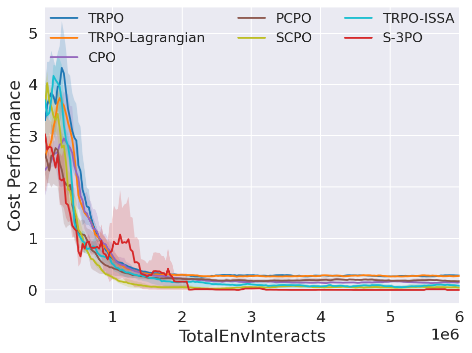
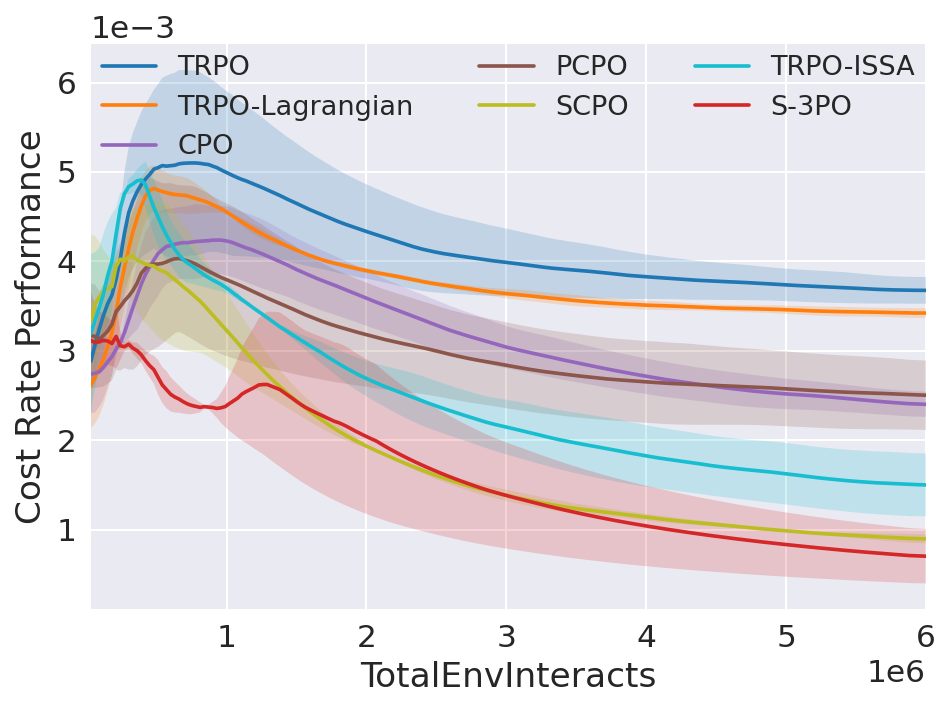
(b) Goal_Point_4Hazard

(c) Goal_Point_8Hazard

Figure 18: Evaluation performance of Goal_Point_Hazard

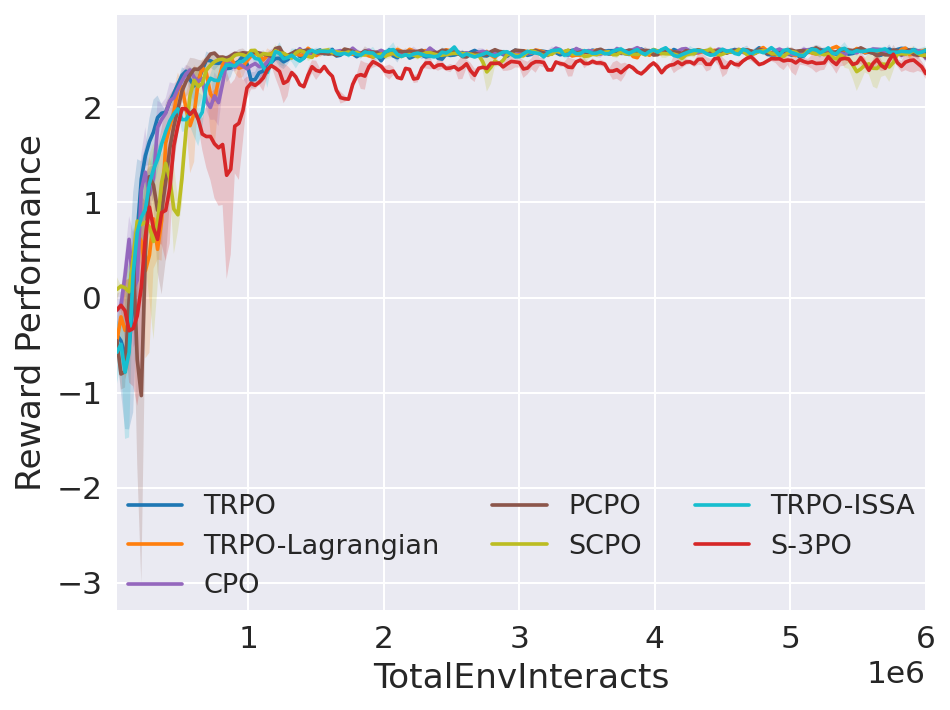
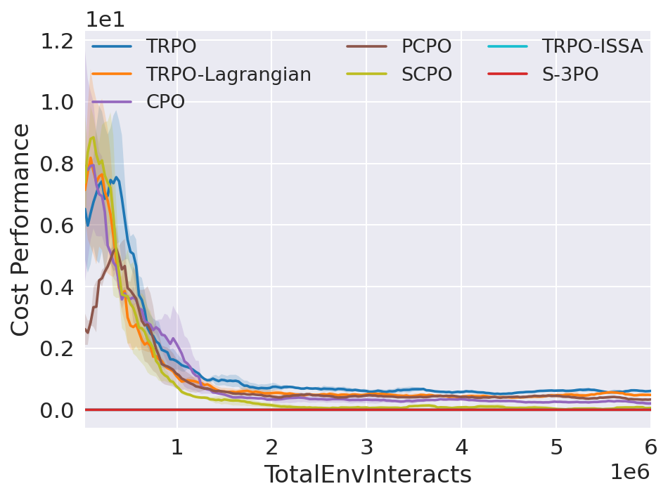
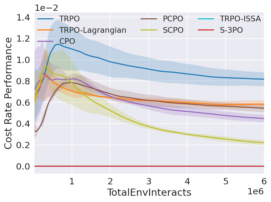
(a) Goal_Point_1Hazard

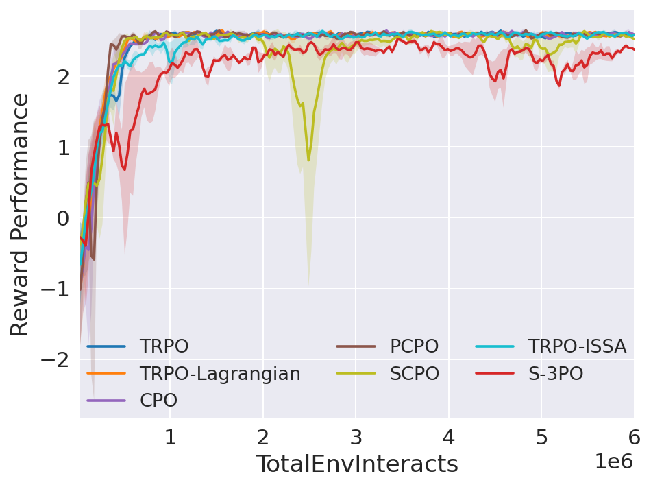
(b) Goal_Point_4Hazard

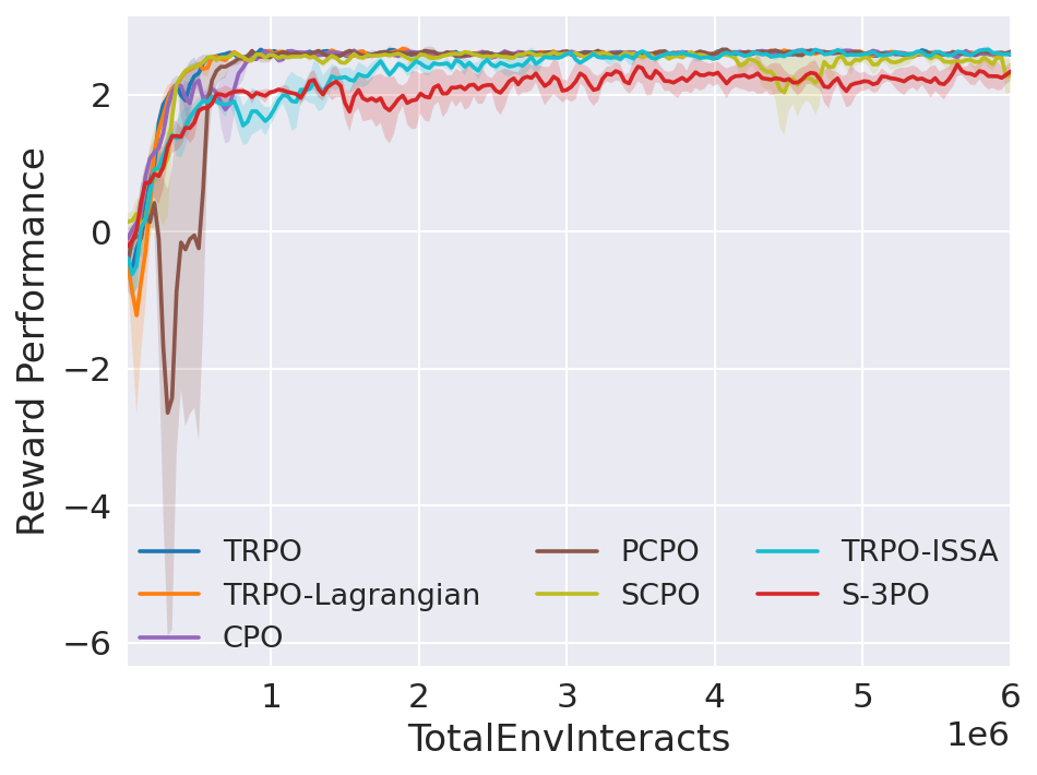
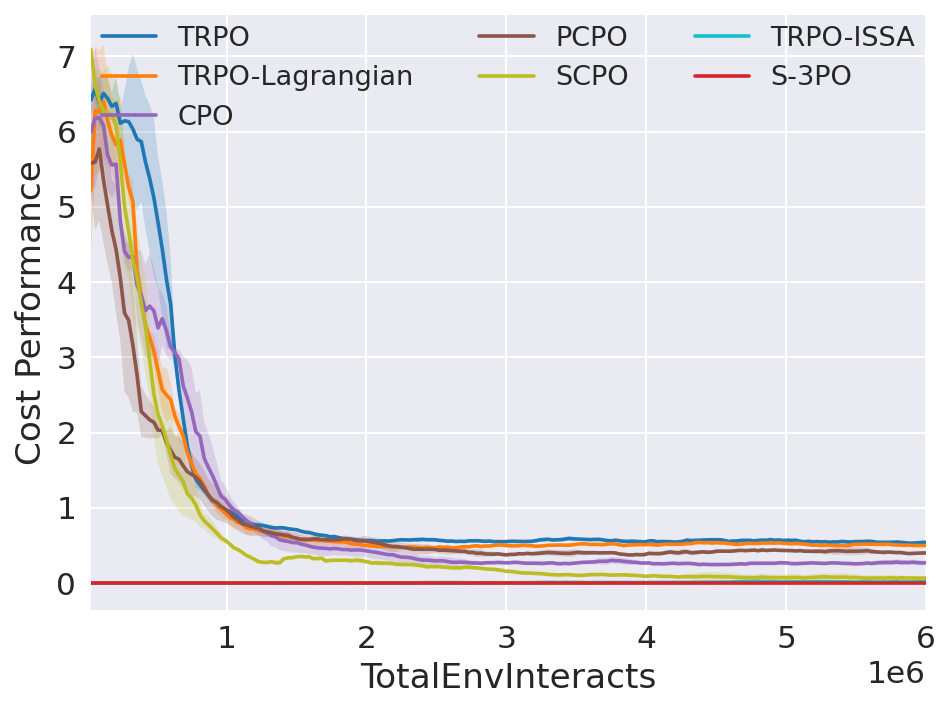
(c) Goal_Point_8Hazard

Figure 20: Training performance of Goal_Point_Hazard

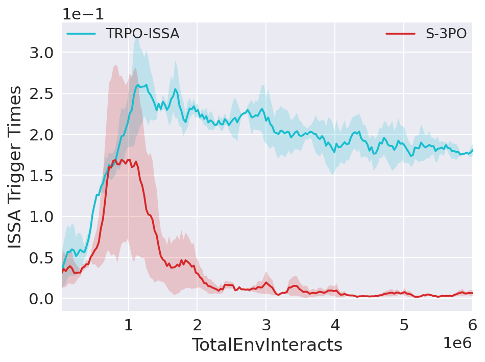
(b) Goal_Point_4Hazard

(c) Goal_Point_8Hazard

Figure 22: ISSA performance of Goal_Point_Hazard

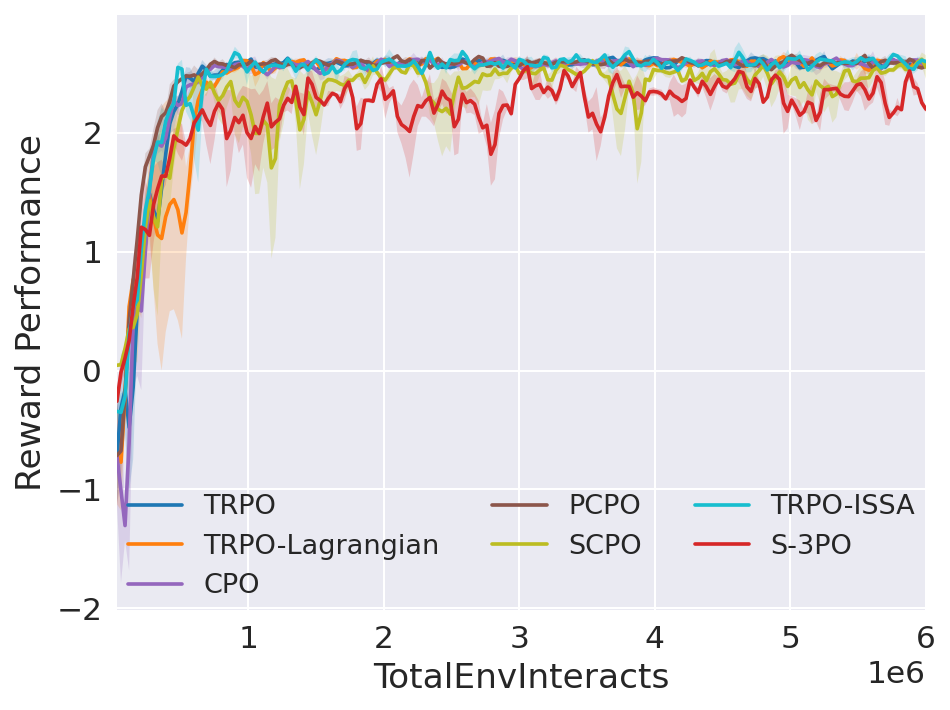
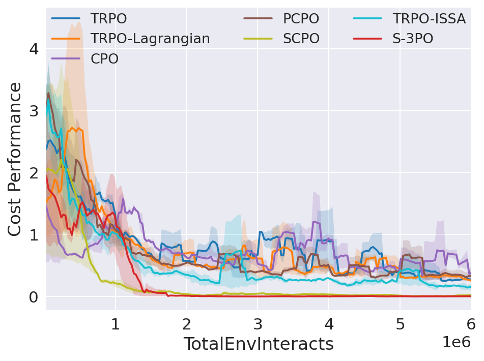
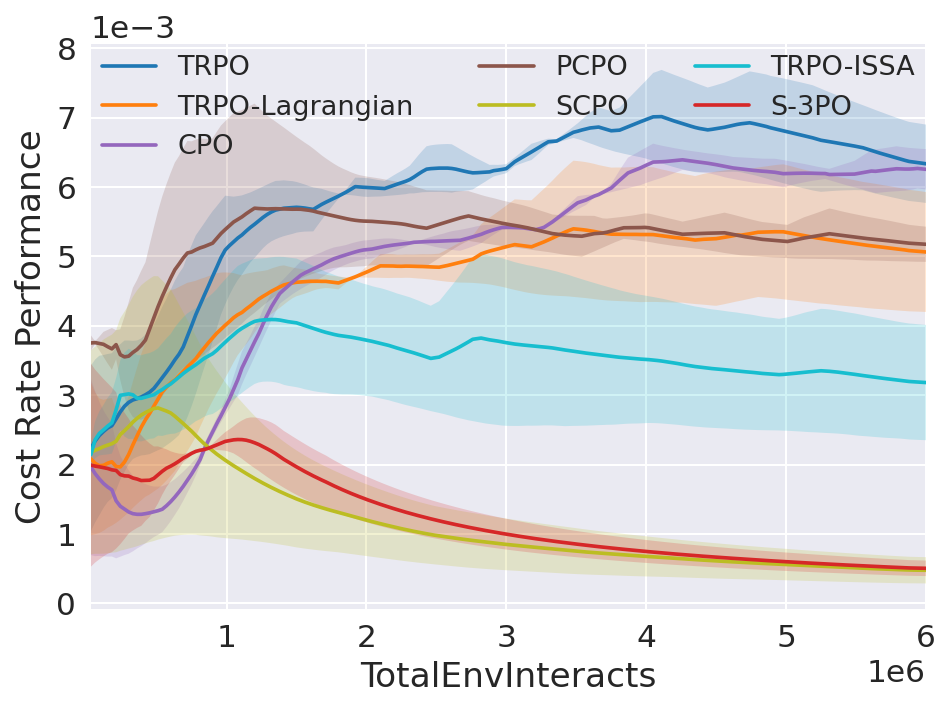
(b) Goal_Point_4Pillar

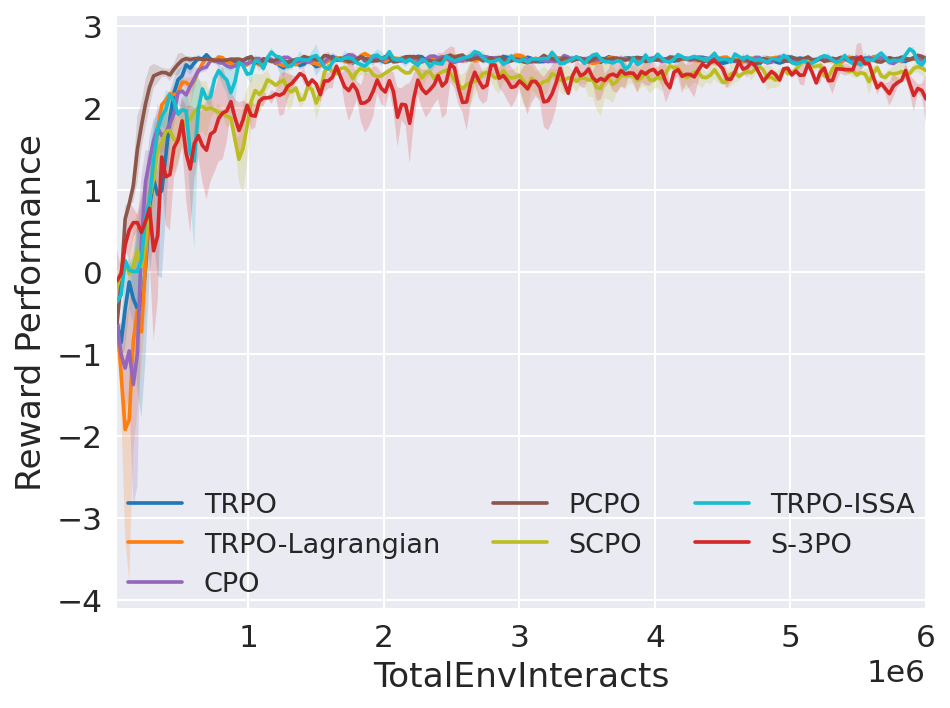
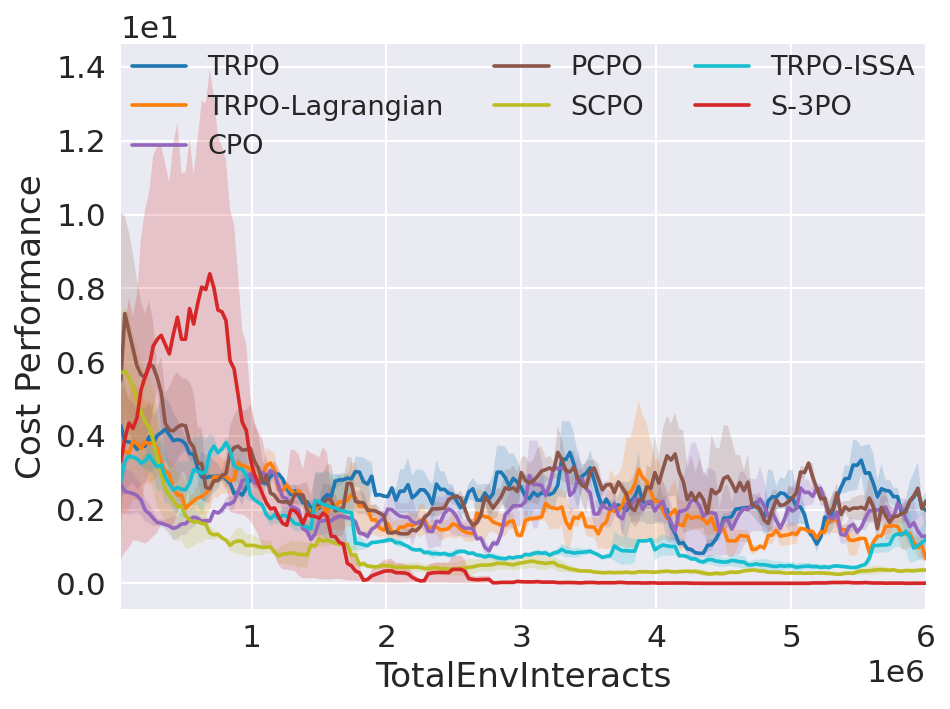
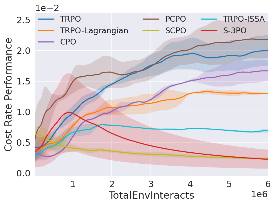
(c) Goal_Point_8Pillar

Figure 24: Evaluation performance of Goal_Point_Pillar

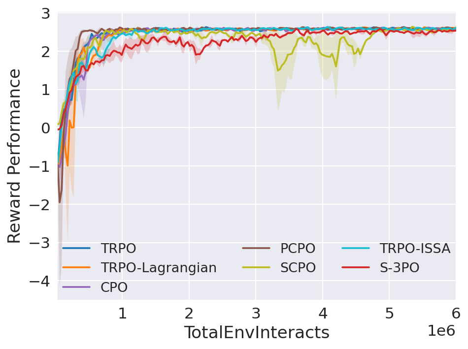
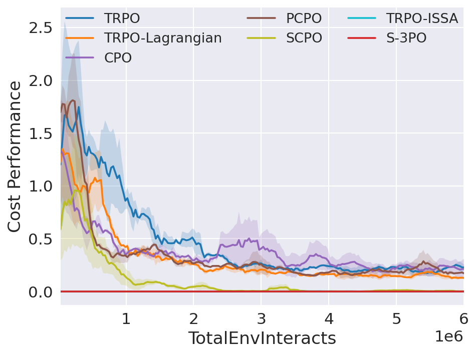
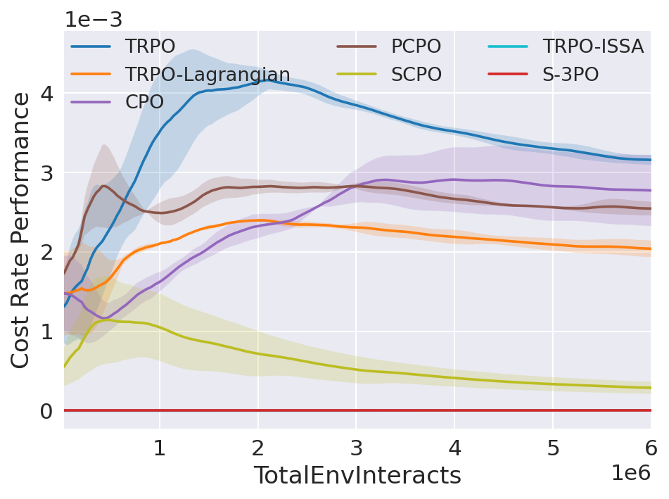
(a) Goal_Point_1Pillar

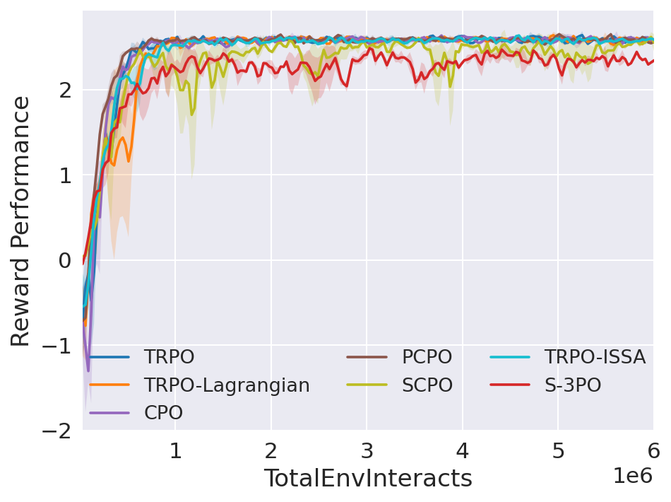
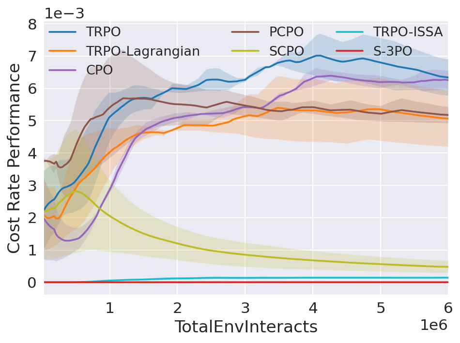
(b) Goal_Point_4Pillar

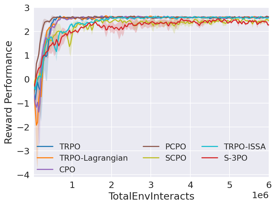
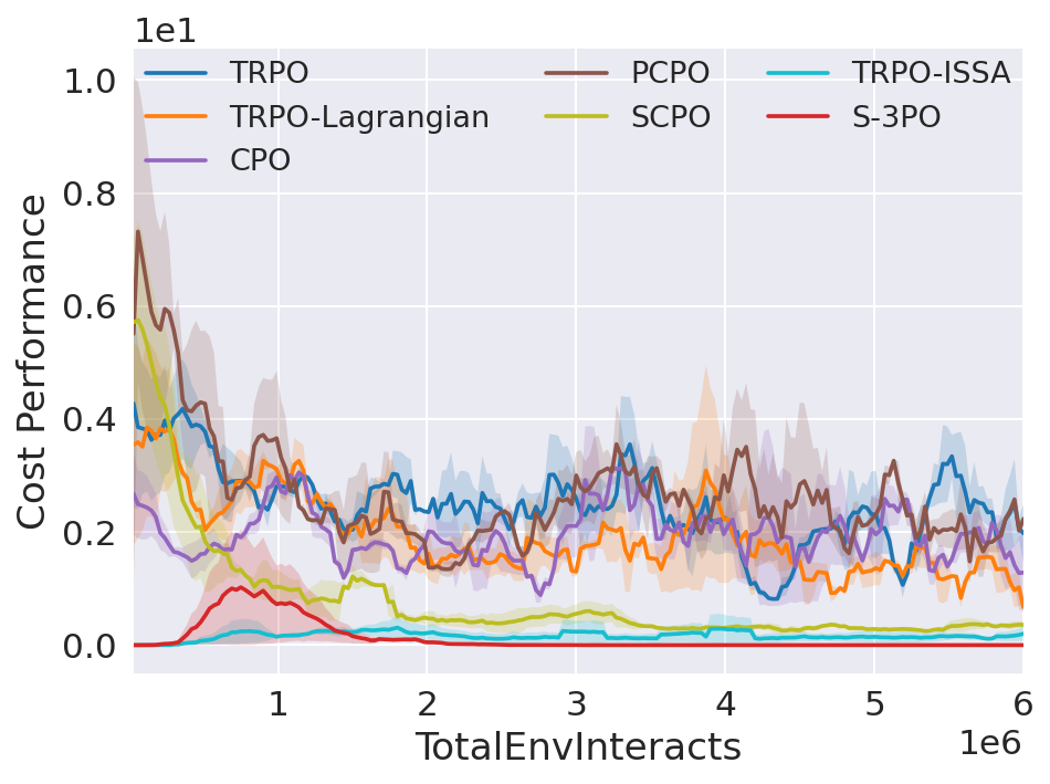
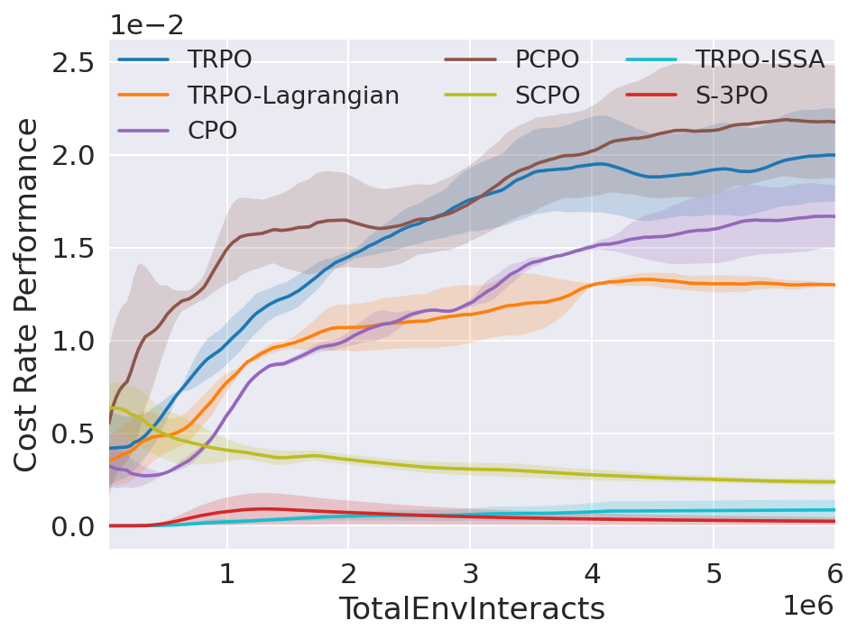
(c) Goal_Point_8Pillar

Figure 26: Training performance of Goal_Point_Pillar

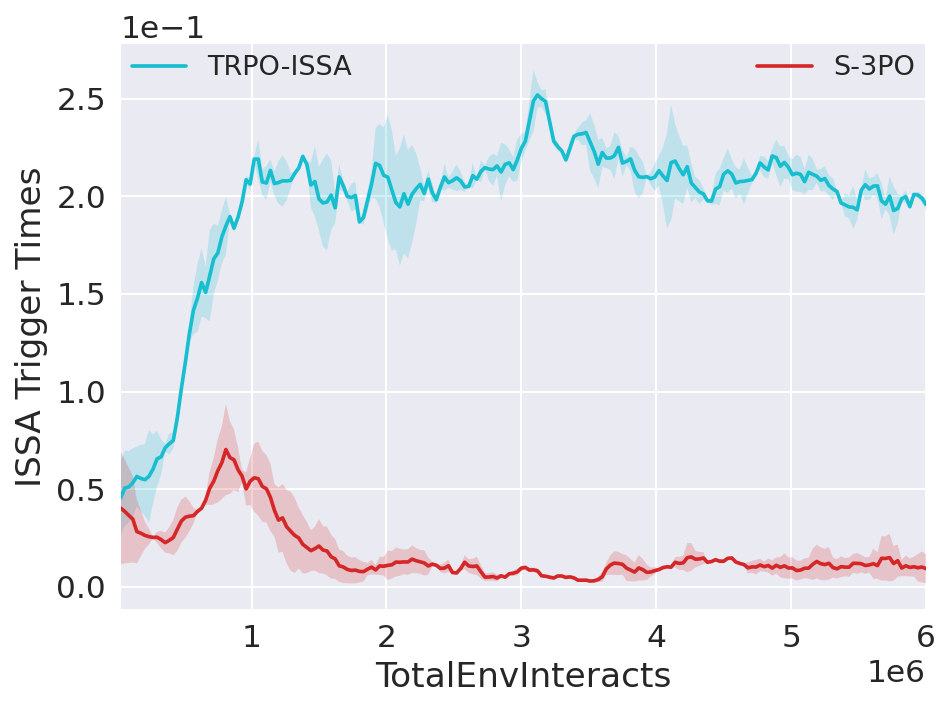
(b) Goal_Point_4Pillar

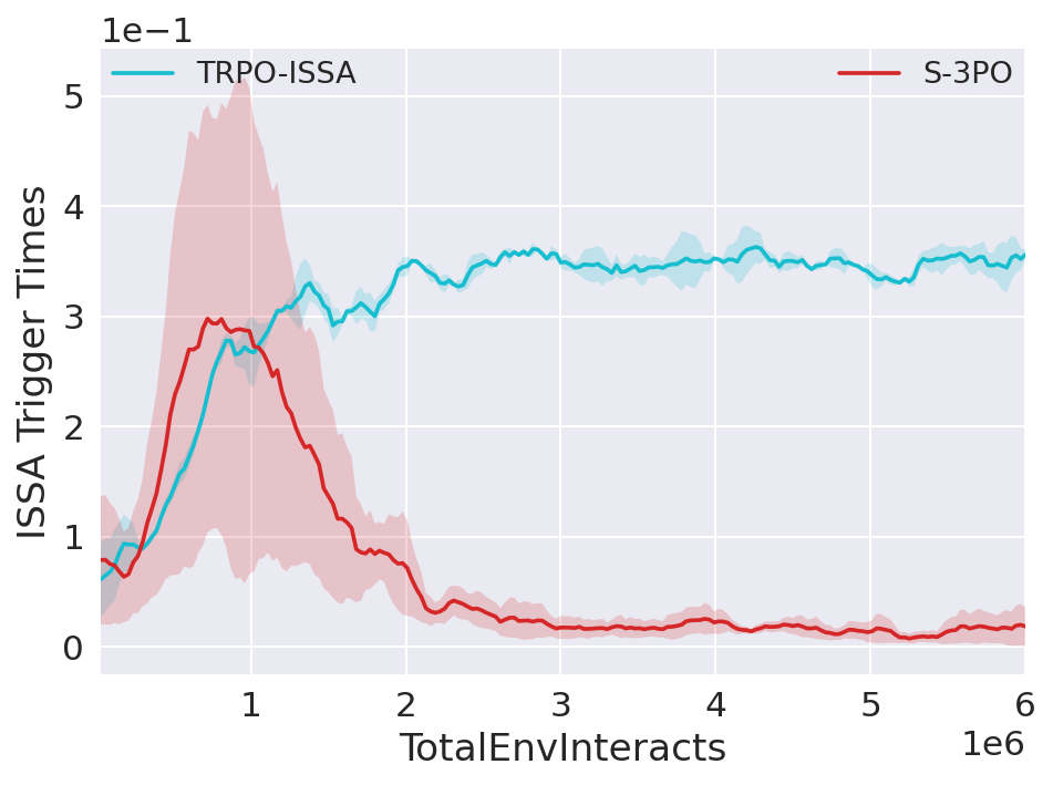
(c) Goal_Point_8Pillar

Figure 28: ISSA performance of Goal_Point_Pillar

Both the evaluation performance and training performance are reported based on the above metrics. Besides, we also report the ISSA triger times as ISSA performance of TRPO-ISSA and S-3PO. All of the metrics were obtained from the final epoch after convergence. Each metric was averaged over two random seed. The evaluation performance curves of all experiments are shown in Figures 18, 24 and 30, the training performance curves of all experiments are shown in Figures 20, 26 and 32 and the ISSA performance curves of all experiments are shown in Figures 22, 28 and 34

Table 5: Metrics of three Goal_Point_Hazard environments obtained from the final epoch.

(a) Goal_Point_1Hazard

Algorithm	Evaluation Performance			Training Performance			ISSA Performance
	$\bar{J}_{r}$	$\bar{M}_{c}$	$\bar{\rho}_{c}$	$\bar{J}_{r}$	$\bar{M}_{c}$	$\bar{\rho}_{c}$
TRPO	2.5738	0.5078	0.0082	2.5738	0.5078	0.0082	-
TRPO-Lagrangian	2.6313	0.5977	0.0058	2.6313	0.5977	0.0058	-
CPO	2.4988	0.1713	0.0045	2.4988	0.1713	0.0045	-
PCPO	2.4928	0.3765	0.0054	2.4928	0.3765	0.0054	-
SCPO	2.5457	0.0326	0.0022	2.5457	0.0326	0.0022	-
TRPO-ISSA	2.5113	0.0000	0.0000	2.5981	0.0000	0.0000	0.2714
S-3PO	2.4157	0.0000	0.0000	2.2878	0.0000	0.0000	0.0285

(b) Goal_Point_4Hazard

Algorithm	Evaluation Performance			Training Performance			ISSA Performance
	$\bar{J}_{r}$	$\bar{M}_{c}$	$\bar{\rho}_{c}$	$\bar{J}_{r}$	$\bar{M}_{c}$	$\bar{\rho}_{c}$
TRPO	2.6098	0.2619	0.0037	2.6098	0.2619	0.0037	-
TRPO-Lagrangian	2.5494	0.2108	0.0034	2.5494	0.2108	0.0034	-
CPO	2.5924	0.1654	0.0024	2.5924	0.1654	0.0024	-
PCPO	2.5575	0.1824	0.0025	2.5575	0.1824	0.0025	-
SCPO	2.5535	0.0523	0.0009	2.5535	0.0523	0.0009	-
TRPO-ISSA	2.5014	0.0712	0.0000	2.5977	0.0135	0.0000	0.1781
S-3PO	2.3868	0.0000	0.0000	2.3550	0.0000	0.0000	0.0117

(c) Goal_Point_8Hazard

Algorithm	Evaluation Performance			Training Performance			ISSA Performance
	$\bar{J}_{r}$	$\bar{M}_{c}$	$\bar{\rho}_{c}$	$\bar{J}_{r}$	$\bar{M}_{c}$	$\bar{\rho}_{c}$
TRPO	2.5535	0.5208	0.0074	2.5535	0.5208	0.0074	-
TRPO-Lagrangian	2.5851	0.5119	0.0064	2.5851	0.5119	0.0064	-
CPO	2.6440	0.2944	0.0041	2.6440	0.2944	0.0041	-
PCPO	2.6249	0.3843	0.0052	2.6249	0.3843	0.0052	-
SCPO	2.5126	0.0703	0.0020	2.5126	0.0703	0.0020	-
TRPO-ISSA	2.5862	0.0865	0.0000	2.5800	0.0152	0.0000	0.3431
S-3PO	2.4207	0.1710	0.0000	2.3323	0.0000	0.0000	0.0337

Table 6: Metrics of three Goal_Pillar_Hazard environments obtained from the final epoch.

(a) Goal_Point_1Pillar

Algorithm	Evaluation Performance			Training Performance			ISSA Performance
	$\bar{J}_{r}$	$\bar{M}_{c}$	$\bar{\rho}_{c}$	$\bar{J}_{r}$	$\bar{M}_{c}$	$\bar{\rho}_{c}$
TRPO	2.6065	0.2414	0.0032	2.6065	0.2414	0.0032	-
TRPO-Lagrangian	2.5772	0.1218	0.0020	2.5772	0.1218	0.0020	-
CPO	2.5464	0.2342	0.0028	2.5464	0.2342	0.0028	-
PCPO	2.5857	0.2088	0.0025	2.5857	0.2088	0.0025	-
SCPO	2.5928	0.0040	0.0003	2.5928	0.0040	0.0003	-
TRPO-ISSA	2.5985	0.0000	0.0000	2.5909	0.0020	0.0000	0.3169
S-3PO	2.5551	0.0000	0.0000	2.5241	0.0000	0.0000	0.0060

(b) Goal_Point_4Pillar

Algorithm	Evaluation Performance			Training Performance			ISSA Performance
	$\bar{J}_{r}$	$\bar{M}_{c}$	$\bar{\rho}_{c}$	$\bar{J}_{r}$	$\bar{M}_{c}$	$\bar{\rho}_{c}$
TRPO	2.5671	0.4112	0.0063	2.5671	0.4112	0.0063	-
TRPO-Lagrangian	2.6040	0.2786	0.0050	2.6040	0.2786	0.0050	-
CPO	2.5720	0.5523	0.0062	2.5720	0.5523	0.0062	-
PCPO	2.5709	0.3240	0.0052	2.5709	0.3240	0.0052	-
SCPO	2.5367	0.0064	0.0005	2.5367	0.0064	0.0005	-
TRPO-ISSA	2.5739	0.1198	0.0001	2.5881	0.0427	0.0001	0.2039
S-3PO	2.2513	0.0114	0.0000	2.3459	0.0000	0.0000	0.0116

(c) Goal_Point_8Pillar

Algorithm	Evaluation Performance			Training Performance			ISSA Performance
	$\bar{J}_{r}$	$\bar{M}_{c}$	$\bar{\rho}_{c}$	$\bar{J}_{r}$	$\bar{M}_{c}$	$\bar{\rho}_{c}$
TRPO	2.6140	3.1552	0.0201	2.6140	3.1552	0.0201	-
TRPO-Lagrangian	2.6164	0.6632	0.0129	2.6164	0.6632	0.0129	-
CPO	2.6440	0.5655	0.0166	2.6440	0.5655	0.0166	-
PCPO	2.5704	6.6251	0.0219	2.5704	6.6251	0.0219	-
SCPO	2.4162	0.2589	0.0024	2.4162	0.2589	0.0024	-
TRPO-ISSA	2.6203	0.6910	0.0009	2.5921	0.0709	0.0009	0.3517
S-3PO	2.0325	0.0147	0.0002	2.3371	0.0000	0.0002	0.0231

Table 7: Metrics of three link robots environments obtained from the final epoch.

(a) Goal_Swimmer_1Hazard

Algorithm	Evaluation Performance			Training Performance			ISSA Performance
	$\bar{J}_{r}$	$\bar{M}_{c}$	$\bar{\rho}_{c}$	$\bar{J}_{r}$	$\bar{M}_{c}$	$\bar{\rho}_{c}$
TRPO	2.7049	0.3840	0.0076	2.7049	0.3840	0.0076	-
TRPO-Lagrangian	2.6154	0.3739	0.0060	2.6154	0.3739	0.0060	-
CPO	2.5817	0.3052	0.0056	2.5817	0.3052	0.0056	-
PCPO	2.5418	0.6243	0.0055	2.5418	0.6243	0.0055	-
SCPO	2.6432	0.3919	0.0051	2.6432	0.3919	0.0051	-
TRPO-ISSA	2.5826	0.2595	0.0000	2.5955	0.0000	0.0000	0.1240
S-3PO	2.6032	0.0313	0.0000	2.6239	0.0001	0.0000	0.0378

(b) Goal_Ant_1Hazard

Algorithm	Evaluation Performance			Training Performance			ISSA Performance
	$\bar{J}_{r}$	$\bar{M}_{c}$	$\bar{\rho}_{c}$	$\bar{J}_{r}$	$\bar{M}_{c}$	$\bar{\rho}_{c}$
TRPO	2.6390	0.3559	0.0074	2.6390	0.3559	0.0074	-
TRPO-Lagrangian	2.5866	0.2169	0.0044	2.5866	0.2169	0.0044	-
CPO	2.6175	0.2737	0.0072	2.6175	0.2737	0.0072	-
PCPO	2.6103	0.2289	0.0076	2.6103	0.2289	0.0076	-
SCPO	2.6341	0.2384	0.0065	2.6341	0.2384	0.0065	-
TRPO-ISSA	2.6509	0.3831	0.0032	2.6318	0.3516	0.0032	0.0279
S-3PO	2.2047	0.0000	0.0002	2.2031	0.0000	0.0002	0.0001

(c) Goal_Walker_1Hazard

Algorithm	Evaluation Performance			Training Performance			ISSA Performance
	$\bar{J}_{r}$	$\bar{M}_{c}$	$\bar{\rho}_{c}$	$\bar{J}_{r}$	$\bar{M}_{c}$	$\bar{\rho}_{c}$
TRPO	2.5812	0.2395	0.0075	2.5812	0.2395	0.0075	-
TRPO-Lagrangian	2.6227	0.1666	0.0041	2.6227	0.1666	0.0041	-
CPO	2.6035	0.3068	0.0062	2.6035	0.3068	0.0062	-
PCPO	2.5775	0.2414	0.0059	2.5775	0.2414	0.0059	-
SCPO	2.6352	0.1423	0.0051	2.6352	0.1423	0.0051	-
TRPO-ISSA	2.6419	0.3544	0.0037	2.5787	0.2060	0.0037	0.0316
S-3PO	2.6117	0.3437	0.0025	2.6055	0.2665	0.0025	0.0319

(a) Goal_Point_1Hazard

(a) Goal_Point_1Hazard

(a) Goal_Point_1Pillar

(a) Goal_Point_1Pillar

(a) Goal_Swimmer_1Hazard

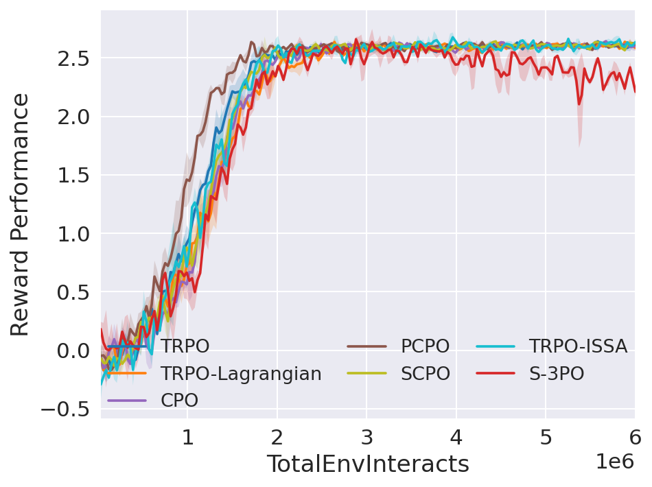
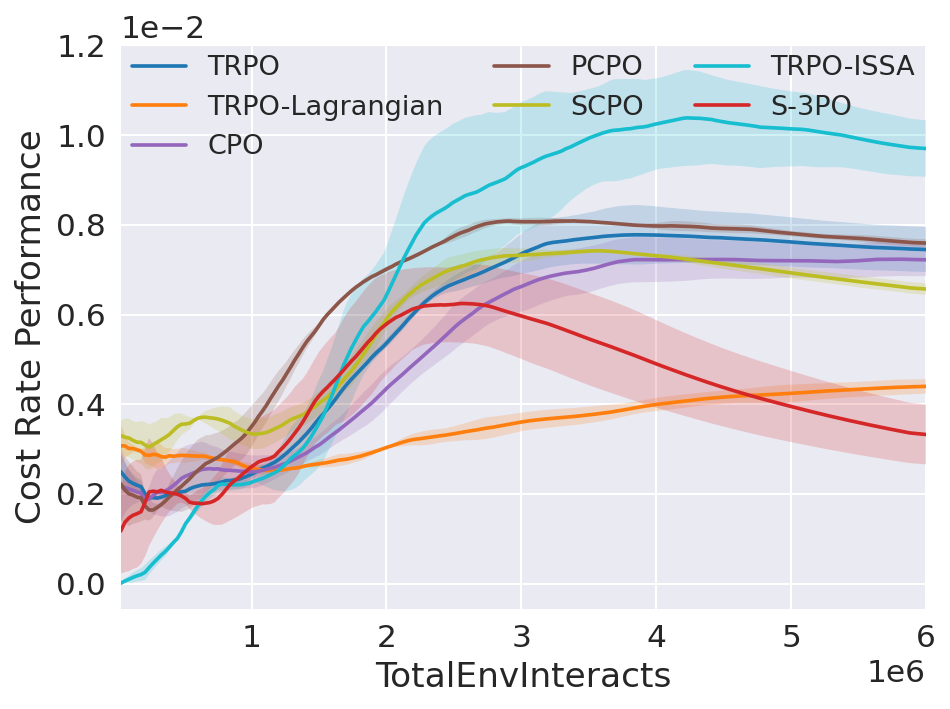
(b) Goal_Ant_1Hazard

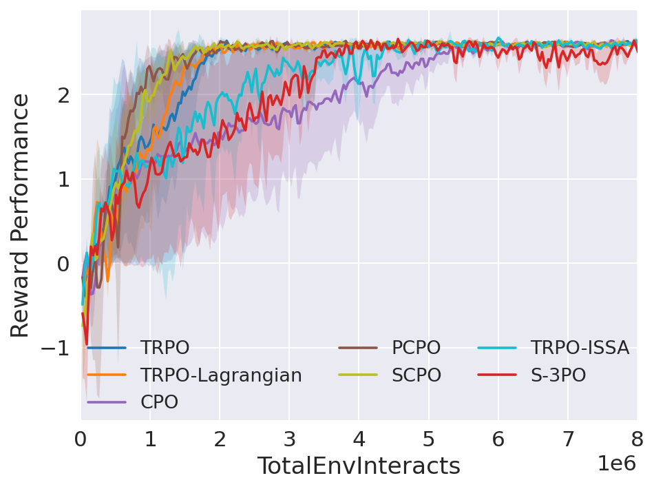
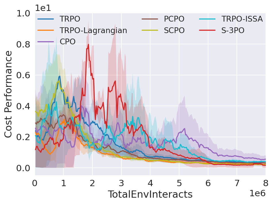
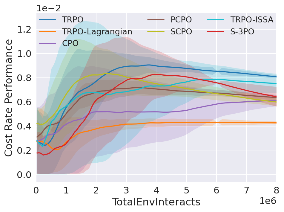
(c) Goal_Walker_1Hazard

Figure 30: Evaluation performance of link robots

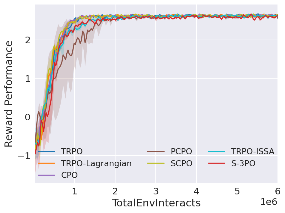
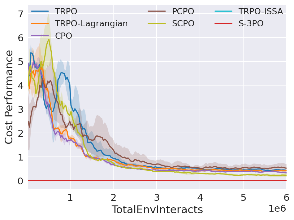
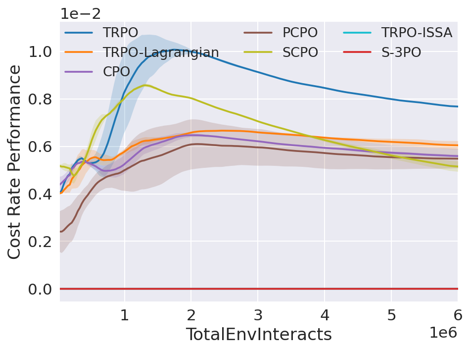
(a) Goal_Swimmer_1Hazard

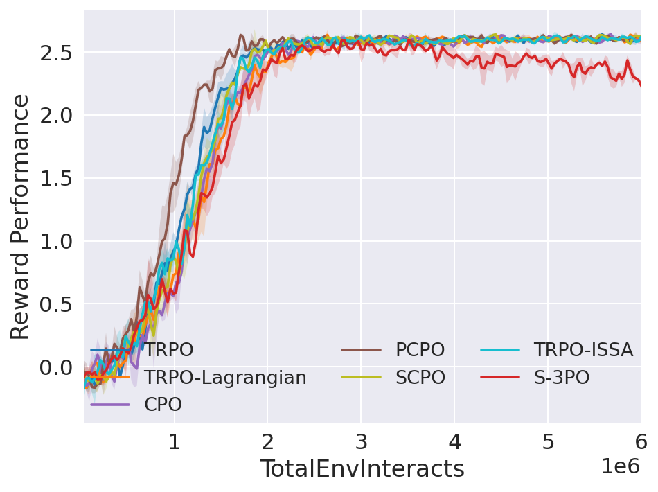
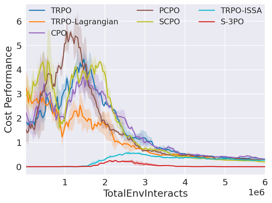
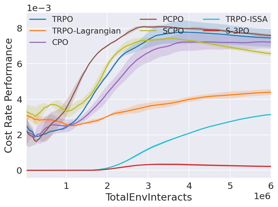
(b) Goal_Ant_1Hazard

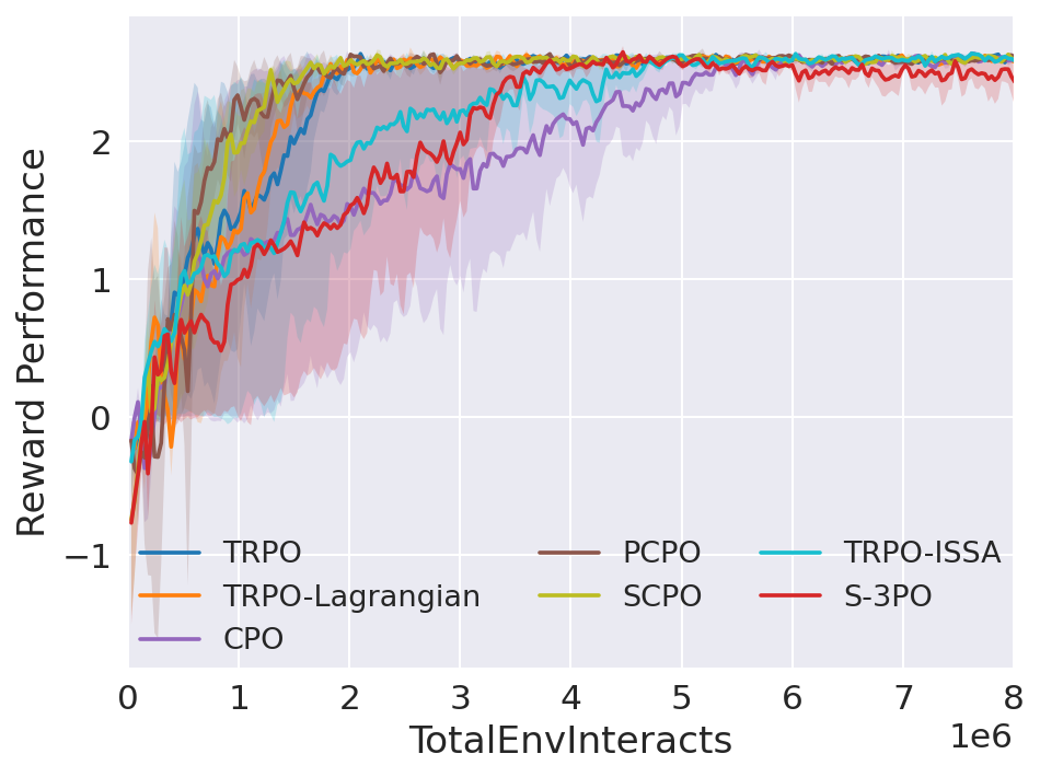
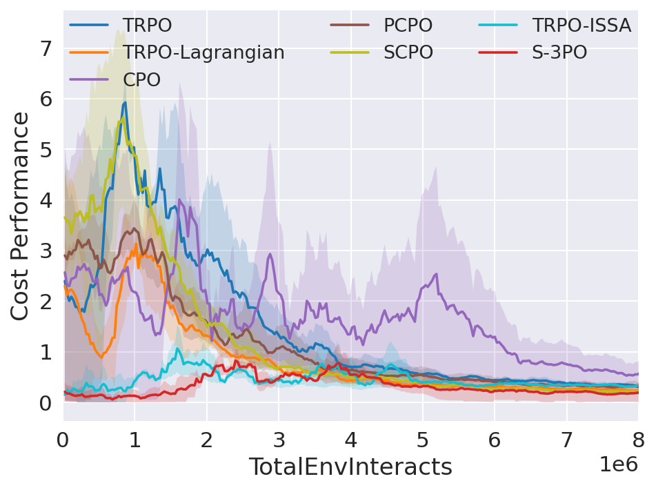
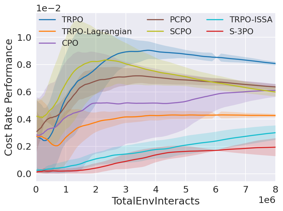
(c) Goal_Walker_1Hazard

Figure 32: Training performance of link robots

(a) Goal_Swimmer_1Hazard

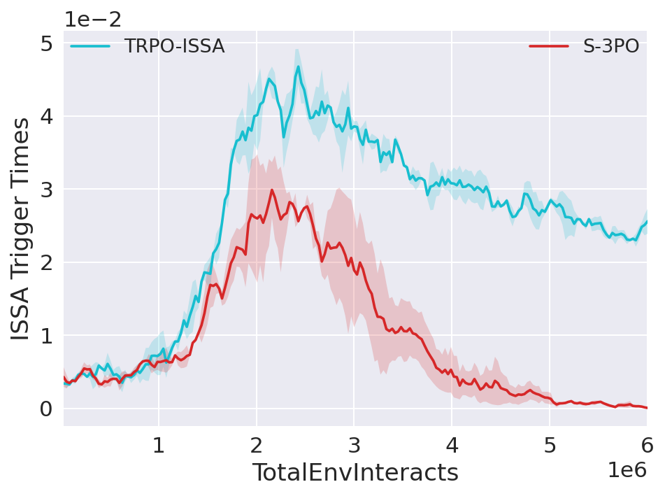
(b) Goal_Ant_1Hazard

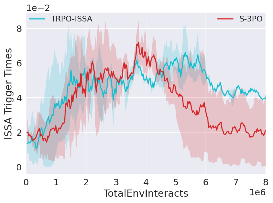
(c) Goal_Walker_1Hazard

Figure 34: ISSA performance of link robots

References

- Achiam et al. (2017) Achiam, J.; Held, D.; Tamar, A.; and Abbeel, P. 2017. Constrained policy optimization. In International conference on machine learning, 22–31. PMLR.
- Ames, Grizzle, and Tabuada (2014) Ames, A. D.; Grizzle, J. W.; and Tabuada, P. 2014. Control barrier function based quadratic programs with application to adaptive cruise control. In 53rd IEEE Conference on Decision and Control, 6271–6278. IEEE.
- Bohez et al. (2019) Bohez, S.; Abdolmaleki, A.; Neunert, M.; Buchli, J.; Heess, N.; and Hadsell, R. 2019. Value constrained model-free continuous control. arXiv preprint arXiv:1902.04623.
- Chen and Liu (2021) Chen, H.; and Liu, C. 2021. Safe and sample-efficient reinforcement learning for clustered dynamic environments. IEEE Control Systems Letters, 6: 1928–1933.
- Dalal et al. (2018) Dalal, G.; Dvijotham, K.; Vecerik, M.; Hester, T.; Paduraru, C.; and Tassa, Y. 2018. Safe exploration in continuous action spaces. CoRR, abs/1801.08757.
- Fisac et al. (2018) Fisac, J. F.; Akametalu, A. K.; Zeilinger, M. N.; Kaynama, S.; Gillula, J.; and Tomlin, C. J. 2018. A general safety framework for learning-based control in uncertain robotic systems. IEEE Transactions on Automatic Control, 64(7): 2737–2752.
- Gracia, Garelli, and Sala (2013) Gracia, L.; Garelli, F.; and Sala, A. 2013. Reactive sliding-mode algorithm for collision avoidance in robotic systems. IEEE Transactions on Control Systems Technology, 21(6): 2391–2399.
- Gu et al. (2022) Gu, S.; Yang, L.; Du, Y.; Chen, G.; Walter, F.; Wang, J.; Yang, Y.; and Knoll, A. 2022. A review of safe reinforcement learning: Methods, theory and applications. arXiv preprint arXiv:2205.10330.
- He et al. (2023) He, S.; Zhao, W.; Hu, C.; Zhu, Y.; and Liu, C. 2023. A hierarchical long short term safety framework for efficient robot manipulation under uncertainty. Robotics and Computer-Integrated Manufacturing, 82: 102522.
- He, Zhao, and Liu (2023) He, T.; Zhao, W.; and Liu, C. 2023. AutoCost: Evolving Intrinsic Cost for Zero-violation Reinforcement Learning. Proceedings of the AAAI Conference on Artificial Intelligence.
- Khatib (1986) Khatib, O. 1986. Real-time obstacle avoidance for manipulators and mobile robots. In Autonomous robot vehicles, 396–404. Springer.
- Liang, Que, and Modiano (2018) Liang, Q.; Que, F.; and Modiano, E. 2018. Accelerated primal-dual policy optimization for safe reinforcement learning. arXiv preprint arXiv:1802.06480.
- Liu and Tomizuka (2014) Liu, C.; and Tomizuka, M. 2014. Control in a safe set: Addressing safety in human-robot interactions. In ASME 2014 Dynamic Systems and Control Conference. American Society of Mechanical Engineers Digital Collection.
- Liu, Halev, and Liu (2021) Liu, Y.; Halev, A.; and Liu, X. 2021. Policy learning with constraints in model-free reinforcement learning: A survey. In The 30th International Joint Conference on Artificial Intelligence (IJCAI).
- Ma et al. (2021) Ma, H.; Liu, C.; Li, S. E.; Zheng, S.; Sun, W.; and Chen, J. 2021. Learn Zero-Constraint-Violation Policy in Model-Free Constrained Reinforcement Learning. arXiv preprint arXiv:2111.12953.
- Noren, Zhao, and Liu (2021) Noren, C.; Zhao, W.; and Liu, C. 2021. Safe Adaptation with Multiplicative Uncertainties Using Robust Safe Set Algorithm. In Modeling, Estimation and Control Conference.
- Ray, Achiam, and Amodei (2019) Ray, A.; Achiam, J.; and Amodei, D. 2019. Benchmarking safe exploration in deep reinforcement learning. CoRR, abs/1910.01708.
- Schulman et al. (2015) Schulman, J.; Levine, S.; Abbeel, P.; Jordan, M.; and Moritz, P. 2015. Trust region policy optimization. In International conference on machine learning, 1889–1897. PMLR.
- Shao et al. (2021) Shao, Y. S.; Chen, C.; Kousik, S.; and Vasudevan, R. 2021. Reachability-based trajectory safeguard (rts): A safe and fast reinforcement learning safety layer for continuous control. IEEE Robotics and Automation Letters, 6(2): 3663–3670.
- Tessler, Mankowitz, and Mannor (2018) Tessler, C.; Mankowitz, D. J.; and Mannor, S. 2018. arXiv preprint arXiv:1805.11074.
- Thananjeyan et al. (2021) Thananjeyan, B.; Balakrishna, A.; Nair, S.; Luo, M.; Srinivasan, K.; Hwang, M.; Gonzalez, J. E.; Ibarz, J.; Finn, C.; and Goldberg, K. 2021. Recovery rl: Safe reinforcement learning with learned recovery zones. IEEE Robotics and Automation Letters, 6(3): 4915–4922.
- Wei et al. (2022) Wei, T.; Kang, S.; Zhao, W.; and Liu, C. 2022. Persistently feasible robust safe control by safety index synthesis and convex semi-infinite programming. IEEE Control Systems Letters, 7: 1213–1218.
- Wei and Liu (2019) Wei, T.; and Liu, C. 2019. Safe control algorithms using energy functions: A unified framework, benchmark, and new directions. In 2019 IEEE 58th Conference on Decision and Control (CDC), 238–243. IEEE.
- Yang et al. (2020) Yang, T.-Y.; Rosca, J.; Narasimhan, K.; and Ramadge, P. J. 2020. Projection-based constrained policy optimization. arXiv preprint arXiv:2010.03152.
- Zhao et al. (2023a) Zhao, W.; Chen, R.; Sun, Y.; Liu, R.; Wei, T.; and Liu, C. 2023a. GUARD: A Safe Reinforcement Learning Benchmark. arXiv preprint arXiv:2305.13681.
- Zhao et al. (2023b) Zhao, W.; Chen, R.; Sun, Y.; Wei, T.; and Liu, C. 2023b. State-wise Constrained Policy Optimization. arXiv preprint arXiv:2306.12594.
- Zhao et al. (2023c) Zhao, W.; He, T.; Chen, R.; Wei, T.; and Liu, C. 2023c. State-wise safe reinforcement learning: A survey. arXiv preprint arXiv:2302.03122.
- Zhao, He, and Liu (2021) Zhao, W.; He, T.; and Liu, C. 2021. Model-free safe control for zero-violation reinforcement learning. In 5th Annual Conference on Robot Learning.
- Zhao, He, and Liu (2022) Zhao, W.; He, T.; and Liu, C. 2022. Probabilistic Safeguard for Reinforcement Learning Using Safety Index Guided Gaussian Process Models. arXiv preprint arXiv:2210.01041.