MatchXML: An Efficient Text-label Matching Framework for Extreme Multi-label Text Classification

Abstract

The eXtreme Multi-label text Classification (XMC) refers to training a classifier that assigns a text sample with relevant labels from an extremely large-scale label set (e.g., millions of labels). We propose MatchXML, an efficient text-label matching framework for XMC. We observe that the label embeddings generated from the sparse Term Frequency-Inverse Document Frequency (TF–IDF) features have several limitations. We thus propose label2vec to effectively train the semantic dense label embeddings by the Skip-gram model. The dense label embeddings are then used to build a Hierarchical Label Tree by clustering. In fine-tuning the pre-trained encoder Transformer, we formulate the multi-label text classification as a text-label matching problem in a bipartite graph. We then extract the dense text representations from the fine-tuned Transformer. Besides the fine-tuned dense text embeddings, we also extract the static dense sentence embeddings from a pre-trained Sentence Transformer. Finally, a linear ranker is trained by utilizing the sparse TF–IDF features, the fine-tuned dense text representations and static dense sentence features. Experimental results demonstrate that MatchXML achieves state-of-the-art accuracy on five out of six datasets. As for the speed, MatchXML outperforms the competing methods on all the six datasets. Our source code is publicly available at https://github.com/huiyegit/MatchXML.

I Introduction

The eXtreme Multi-label text Classification (XMC) refers to learning a classifier that can annotate an input text with the most relevant labels from an extremely large-scale label set (e.g., millions of labels). This problem has many real world applications, such as labeling a Wikipedia page with relevant tags [1], providing a customer query with related products in product search [2], and recommending the relevant items to a customer in recommendation systems [3].

To address the issue of the extremely large output space in XMC, the Hierarchical Label Tree (HLT) [2] is proposed to effectively reduce the computational complexity from $O(L)$ to $\log(L)$, where $L$ is the number of labels. Taking label embeddings as input, an HLT can be constructed by some partition algorithms [2, 4] based on the K-means clustering. Prior works [2, 4, 5, 6, 7] have applied the Positive Instance Feature Aggregation (PIFA) to compute label embeddings, where one label embedding is the summation of the TF–IDF features of the text samples when this label is positive. However, the label embeddings generated from PIFA have several limitations. First, current machine learning approaches are more efficient to process the data of small dense vectors than the large sparse vectors. Second, the TF–IDF features of the text data is a prerequisite for the PIFA to generate the label embeddings, which may not be always available and thus limits PIFA’s applications. Inspired by the word2vec [8, 9] in training word embeddings, we propose label2vec to learn the semantic dense label embeddings. We consider a set of labels assigned to a text sample as an unordered sequence, where each label can be treated as one word/token. We apply the Skip-gram model [8, 9] to train the embedding for each label. The label2vec approach has better generalization as it does not require to provide TF–IDF features. Besides, the dense label embeddings have smaller storage size and are more efficient to process by the downstream machine learning algorithms. Our experiments demonstrate that the dense label embeddings can better capture the semantic label relationships to generate an HLT than the sparse label embeddings, leading to better performance in the downstream XMC task.

Most of early works [10, 11, 12, 13, 14, 15, 16, 2, 17, 18, 19, 20, 21, 22] leverage the statistical bag-of-words (BOW) or Term Frequency-Inverse Document Frequency (TF–IDF) features as the text representations to train a text classifier. This type of text features is simple yet effective, but it can not capture the semantic meaning of the text document due to the ignorance of word order. Recent works [23, 24, 6, 25, 5] explore deep learning approaches to learn the dense vectors as the text representations. These methods are developed to make use of contextual information of words in text corpora. Therefore, the dense text representations usually lead to better classification accuracy. On the other hand, the recently proposed XR-Transformer [7] and CascadeXML [26] have showed that the sparse TF–IDF features and dense text features are not mutually exclusive to each other, but rather can be leveraged together as the text representations to boost the performance. Inspired by the strategy of XR-Transformer, we obtain the final text representations by taking advantage of sparse TF–IDF features and dense vector features. In addition, we propose a novel approach to improve the quality of dense vector features for XMC. That is, in the fine-tuning stage of the pre-trained Encoder Transformer, we formulate the multi-label text classification as a text-label matching problem in a bipartite graph. Through text-label alignment and label-text alignment in a bipartite graph, the fine-tuned Transformer can yield robust and effective dense text representations. Besides the dense text representations fine-tuned from the above method, we also utilize the static dense sentence embeddings obtained from pre-trained Sentence Transformers, which are widely used in many NLP tasks, such as classification, clustering, retrieval, paraphrase detection and semantic textual similarity. Compared with the sparse TF-IDF representations, the static dense sentence embeddings can capture the semantic meaning and facilitate downstream applications. We extract the static sentence embeddings from the Sentence-T5  [27] and integrate them into our MatchXML approach. We have found that this approach is very effective as shown in our ablation study.

The remainder of the paper is organized as follows. In Section II, we review the related works from the perspectives of extreme classification, cross-modal learning and contrastive learning. The proposed method MatchXML is presented in Section III, where its main components: label2vec, hierarchical label tree, text-label matching and linear ranker are introduced. Experimental results on six benchmark datasets are presented in Section IV, with comparisons to other algorithms currently in the literature. Conclusions and future work are discussed in Section V.

II Related Works

Extreme classification. A great number of works have been proposed to solve the extreme classification problem [28, 19, 29, 30, 31, 32, 33, 22, 34, 35, 21, 36, 37, 38, 39, 40, 41, 42, 43, 44, 45, 46, 47], which can be categorized to One-vs-All approaches, tree-based approaches, embedding-based approaches and deep learning approaches. The One-vs-All approaches, such as PDSparse [13], train one classifier for each label independently to improve classification accuracy. To speed up the computation, these approaches leverage the negative sampling and parallel computing to distribute the training over multiple cores or servers. The tree-based approaches, such as FastXML [10], train a hierarchical tree structure to divide the label set into small groups. These approaches usually have the advantage of fast training and inference. The embedding-based approaches, such as SLEEC [11], seek to lower the computational cost by projecting the high-dimensional label space into the low-dimensional one. However, information loss in the compression process undermines the classification accuracy.

Deep learning approaches leverage the raw text to learn semantic dense text representations instead of the statistical TF-IDF features. Recent works (e.g., X-Transformer [5], APLC-XLNet [25], LightXML [6]) fine-tune the pre-trained Encoder Transformers, including BERT [48], RoBERTa [49] and XLNet [50], to extract the dense text features. Besides, the clustering structure or shallow hierarchical tree structure is designed to deal with the large output label space rather than the traditional linear classifier layer. XR-Transformer [7] proposes a shallow balanced label tree to fine-tune the pre-trained Encoder Transformer in multiple stages. The dense vectors extracted from the last fine-tuning stage and sparse TF-IDF features are leveraged to train the final classifier. Compared with XR-Transformer, we generate the Hierarchical Label Tree by the label embeddings learned from label2vec rather than the TF-IDF features. Besides, we formulate the text classification problem as a text-label matching problem to learn the improved text representations in the fine-tuning stage. Furthermore, we extract the static dense sentence embeddings from the pre-trained Sentence Transformer for the classification task.

Cross-Modal Learning. In the setting of text-label matching, we consider the input texts (i.e., sentence one, sentence two) as the text modality, while the class labels (i.e., 1, 2, 3) as another number modality. Therefore, the line of prior research in cross-modal learning is relevant to our text-label matching approach. The tasks of cross-modal learning involve processing data across different modalities, such as text, image, audio, and video. Some typical Image-Text Matching tasks have been well studied in recent years, including Image-Text Retrieval [51, 52], Visual Question Answering [53, 54] and Text-to-Image Generation [55, 56, 57, 58, 59]. The general framework is to design one image encoder and one text encoder to extract the visual representations and textual representations, respectively, then fuse the cross-modal information to capture the relationships between them. In contrast to the framework of Image-Text Matching, we develop one text encoder for the text data and one embedding layer to extract the dense label representations. Furthermore, the relationship between image and text in Image-Text Matching usually belongs to an one-to-one mapping, while the relationship between text and label is many-to-many in multi-label text classification.

Contrastive Learning. Another line of research in contrastive learning is also related to our proposed method. Recently, self-supervised contrastive learning [60, 61, 62] has attracted great attention due to its remarkable performance in visual representation learning. Typically, a positive pair of images is constructed from two views of the same image, while a negative pair of images is formed from the views of different images. Then a contrastive loss is designed to push together the representations of positive pairs and push apart the ones of negative pairs. Following the framework of self-supervised contrastive learning, supervised contrastive learning [63] constructs additional positive pairs by utilizing the label information. The application of the supervised contrastive loss can be found in recent works [64, 65, 66, 67] to deal with text classification. In this paper, we leverage the supervised constrastive loss as the training objective for text-label matching, and we develop a novel approach to construct the positive and negative text-label pairs for XMC. MACLR [67] is a recent work that applies the contrastive learning for the Extreme Zero-Shot Learning, and thus is related to our MatchXML. First, the contrastive learning paradigm in MACLR belongs to self-supervised contrastive learning, while MatchXML is a supervised contrastive learning method. Specifically, MACLR constructs the positive text-text pair, where the latter text is a sentence randomly sampled from a long input sentence, while MatchXML constructs the positive text-label pair, where the label is one of the class labels of the input text. Secondly, MACLR utilizes the Inverse Cloze Task which is a frequently used pre-training task for the sentence encoder, while MatchXML is derived from the Cross-Modal learning task.

III Method

III-A Preliminaries

Given a training dataset with $N$ samples $\{(x_{i},y_{i})\}_{i=1}^{N}$, where $x_{i}$ denotes the text sample $i$ and $y_{i}$ is ground truth, which can be the expressed as the label vector with binary values 0 and 1. Let $y_{il}$, for $l\in\{1,\cdots,L\}$, denote the $l$th element of $y_{i}$, where $L$ is the cardinality of the label set. When $y_{il}=1$, label $l$ is relevant to text $i$, and not otherwise. In a typical XMC problem, the number of instances $N$ and the number of labels $L$ can be at the order of millions or even larger. The objective of XMC is to learn a classifier $f(x,l)$ from the training dataset, where the value of $f$ indicates the relevance score of text $x$ and label $l$, with a hope that $f$ can generalize well on test dataset $\{(x_{j},y_{j})\}_{j=1}^{N_{t}}$ with high accuracy and fast inference speed.

The training of MatchXML consists of four steps. In the first step, we train the dense label vectors by our proposed label2vec. In the second step, a preliminary Hierarchical Label Tree (HLT) is constructed using a Balanced K-means Clustering algorithm [4]. In the third step, a pre-trained Transformer model is fine-tuned recursively from the top layer to bottom layer through the HLT. Finally, we train a linear classifier by utilizing all three text representations: (1) sparse TF-IDF text features, (2) the dense text representations extracted from the fine-tuned Transformer, and (3) the static dense sentence features extracted from the pre-trained Sentence Transformer. As for the inference, the computational cost contains the feature extraction of input text from the fine-tuned Transformer and the beam search guided by the trained linear classifier through the refined HLT. Thus, the computational complexity of MatchXML inference can be expressed as

$$O(T_{1}+k_{b}d\log(L)),$$ (1)

where $T_{1}$ denotes the cost of extracting the dense text representation from the text encoder, $k_{b}$ is the size of beam search, $d$ is the dimension of the concatenated text representation. The details of MatchXML are elaborated as follows.

III-B label2vec

The Hierarchical Label Tree (HLT) plays a fundamental role in reducing the computational cost in XMC, while the high-quality label embeddings is critical to construct an HLT that can cluster the semantically similar labels together. In this section, we introduce label2vec to train the semantic dense label embeddings for the HLT. We note that the training label set $\{y_{i}\}_{i=1}^{N}$ contains a large amount of semantic information among labels. We therefore treat the positive labels in $y_{i}$ as a label sequence, just like the words/tokens in one sentence in word2vec. Then we adopt the Skip-gram model to train the label embeddings, which can effectively learn high-quality semantic word embeddings from large text corpora. The basic mechanism of the Skip-gram model is to predict the context words from the target word. The training objective is to minimize the following loss function:

$$-\log\sigma(w_{t}^{T}w_{c})-\sum_{i=1}^{k}E_{z_{i}\sim Z_{T}}\left[\log\sigma(-w_{t}^{T}w_{z_{i}})\right],$$ (2)

where $w_{t}$ and $w_{c}$ denote the input vector of target word and context word vector, respectively, and $z_{i}$ is one of the $k$ negative samples. To have the Skip-gram model adapt to the label2vec task, we simply make several necessary modifications as follows. First, in word2vec the $2n_{k}$ training target-context word pairs can be generated by setting a window size to $n_{k}$, consisting of $n_{k}$ context words before and after the target word. Basically, a small window size (i.e., $n_{k}$=2) tends to have the target word focus more on the nearby context words, while a large window size (i.e., $n_{k}$=10) can capture the semantic relationship between the target word and broad context words. The strategy of dynamic window size is adopted in the Skip-gram model to train word2vec. However, in label2vec there is no distance constraint between the target label and its context labels, since they have the semantic similarity if two labels co-occur in one training sample. Therefore, we set the window size $n_{k}$ to be the maximum number of labels among all training samples. Secondly, the subsampling technique is leveraged to mitigate the imbalance issue between the frequent and rare words in word2vec, as the frequent/stop words (e.g., “in”, “the”, and “a”) do not provide much semantic information to train word representations. In contrast, the frequent labels are usually as important as rare labels in XMC to capture the semantic relationships among labels in label2vec. Therefore, we do not apply the subsampling to the frequent labels in label2vec.

III-C Hierarchical Label Tree

Once we train the dense label vectors $W=\{w_{i}\}_{i=1}^{L}$ from $\{y_{i}\}^{N}_{i=1}$ with label2vec, we build a Hierarchical Label Tree (HLT) of depth $D$ from the label vectors $W$ by a Balanced K-means Clustering algorithm [4]. In the construction of HLT, the link relationships of nodes between two adjacent layers are organized as 2D matrices $C=\{C^{t}\}_{t=1}^{D}$ based on the clustering assignments. Then the ground truth label assignment of $t$-th layer $Y^{(t)}$ can be generated by the $(t+1)$-th layer $Y^{(t+1)}$ as follows:

$$Y^{(t)}=binarize(Y^{(t+1)}C^{(t+1)}).$$ (3)

The original ground truth $y_{i}$ corresponds to $Y^{(D)}$ in the bottom layer, then the ground truth label assignment $Y^{(t)}$ can be inferred from the bottom layer to the top according to Eq. 3. Subsequently, we fine-tune the pre-trained Transformer in multiple stages from the top layer to the bottom layer through the HLT.

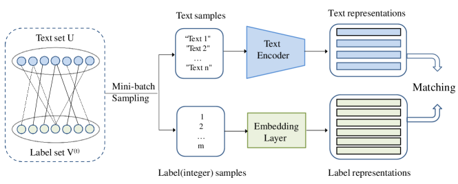
Figure 1: Architecture of text-label matching in a bipartite graph. In fine-tuning the pre-trained Encoder Transformer for the t-th layer of the Hierarchical Label Tree, we consider the input text set U(i.e. training samples X) as the text modality, while the label set $V^{(t)}$ (i.e. training labels $Y^{(t)}$) of the positive integer number format as another number modality.

III-D Text-label Matching

In this section, we present our text-label matching framework for XMC. In the fine-tuning stage, we consider the multi-label classification as a text-label matching problem. We model this matching problem in a bipartite graph $G(U,V^{(t)},E)$, where $U$ and $V^{(t)}$ denote a set of text samples and labels in the $t$-th layer, respectively, and $E$ is a set of edges connecting $U$ and $V^{(t)}$. If text $i$ has a positive label $j$, edge $e_{ij}$ is created between them. Figure 1 illustrates the framework of our approach. During training, we sample a mini-batch of training data, from which the text samples are fed to a text encoder to extract the text representations, and the corresponding labels are fed to an embedding layer to extract the label representations. We consider the text-label matching problem from two aspects: text-label alignment and label-text alignment.

Text-label alignment. In the text-label matching setting, one text sample aligns with multiple positive labels and contrasts with the negative labels in the mini-batch. We construct the set with multiple positive text-label pairs $\{(z_{i},e_{p})\}$, where $p$ is a positive label of text $i$. Following the previous work [7], we also mine the hard negative labels (e.g., negative labels with high output scores) to boost the performance. We then generate the set with a number of negative text-label pairs $\{(z_{i},e_{n})\}$, where $n$ is one of hard negative labels of text $i$. We utilize the dot product $(z_{i},e_{j})$ as the quantitative metric to measure the alignment of the text-label pair. To align the text with labels, we train our model to maximize the alignment scores of positive text-label pairs and minimize the ones of negative text-label pairs. The training objective of text-label alignment is defined as

$$\mathcal{L}_{tl}=\frac{1}{N_{b}}\sum_{i=1}^{N_{b}}\frac{1}{|P_{1}(i)|}\sum_{p\in P_{1}(i)}-\log\frac{\exp((z_{i},e_{p})/\tau)}{\displaystyle\sum_{a\in A_{1}(i)}\exp((z_{i},e_{a})/\tau)},$$ (4)

where ${N_{b}}$ denotes the batch size, $P_{1}(i)$ is the set of indices of positive labels related to text $i$, $|P_{1}(i)|$ is its cardinality, $A_{1}(i)$ is the set of indices of positive and negative labels corresponding to text $i$, and $\tau\in R^{+}$ is a scalar temperature parameter.

Label-text alignment. We also consider the label-text alignment in a reverse way for the text-label matching problem. In the text-label alignment discussed above, we mine a number of hard negative labels for each text to benefit the training process. On the contrary, if we form the label set by combining all the positive labels and hard negative labels within the mini-batch, the computational cost is likely to increase much due to the large cardinality of the label set. To reduce the computational cost, we construct the label set only from all the positive labels within a mini-batch. Similar to the previous text-label alignment, one label sample corresponds with several text samples and contrasts with the remaining text samples in the mini-batch. We generate the set with several positive label-text pairs $\{(e_{i},z_{p})\}$, where $i$ is a positive label for text $p$. Otherwise, they form the set with a number of negative label-text pairs $\{(e_{i},z_{n})\}$, where $i$ is a negative label for text $n$. To align the label with texts, we train our model to maximize the alignment scores of positive label-text pairs and minimize the ones of negative label-text pairs. Similarly, the training objective of label-text alignment is defined as

$$\mathcal{L}_{lt}=\frac{1}{M}\sum_{i=1}^{M}\frac{1}{|P_{2}(i)|}\sum_{p\in P_{2}(i)}-\log\frac{\exp((e_{i},z_{p})/\tau)}{\displaystyle\sum_{a\in A_{2}(i)}\exp((e_{i},z_{a})/\tau)},$$ (5)

where $M$ is the number of positive labels in the mini-batch, $P_{2}(i)$ is the set of indices of positive text samples related to label $i$, $|P_{2}(i)|$ is its cardinality, and $A_{2}(i)$ is the set of indices of text samples within the mini-batch.

Loss function. The overall loss function for text-label matching problem can be the linear combination of the two terms defined above

$$\mathcal{L}=\lambda\mathcal{L}_{tl}+(1-\lambda)\mathcal{L}_{lt},$$ (6)

with $\lambda$ $\in[0,1]$. Experiments show that the setting of hyperparameter $\lambda$ has a notable impact on the performance of MatchXML, and we thus tune it for different datasets.

TABLE I: Statistics of datasets. $N_{train}$ is the number of training samples, $N_{test}$ is the number of test samples, $D$ is the dimension of feature vector, $L$ is the cardinality of label set, $\bar{L}$ is the average number of labels per sample, $\hat{L}$ is the average samples per label.

Dataset $N_{train}$ $N_{test}$ $D$ $L$ $\bar{L}$ $\hat{L}$ EURLex-4k 15,449 3,865 186,104 3,956 5.30 20.79 AmazonCat-13k 1,186,239 306,782 203,882 13,330 5.04 448.57 Wiki10-31k 14,146 6,616 101,938 30,938 18.64 8.52 Wiki-500k 1,779,881 769,421 2,381,304 501,070 4.75 16.86 Amazon-670k 490,449 153,025 135,909 670,091 5.45 3.99 Amazon-3M 1,717,899 742,507 337,067 2,812,281 36.04 22.02

Algorithm 1 MatchXML Training

0:  Training dataset $\{X,Y\}=\{(x_{i},y_{i})\}_{i=1}^{N}$, TF-IDF features $\{\bar{X}\}=\{(\bar{x}_{i})\}_{i=1}^{N}$, static dense sentence embeddings $\{\check{X}\}=\{(\check{x}_{i})\}_{i=1}^{N}$, Skip-gram model $h$, text encoder $g$, the depth of HLT $D$

0:  Optimized text encoder $g$ and the hierarchical linear ranker $\{{R}^{(t)}\}_{t=1}^{{D}}$

1:  Generate label pairs $\{(l_{i}^{k},l_{j}^{k})\}_{k=1}^{K}$ from $\{Y\}=\{y_{i}\}_{i=1}^{N}$

2:  for {1, $\cdots$, # of training epochs} do

3:      for {1, $\cdots$, # of training steps} do

4:        Sample a mini-batch of label pairs $\{(l_{i},l_{j})\}$

5:        Update Skip-gram model $h$ to minimize Eq. 2

6:     end for

7:  end for

8:  Obtain dense label vectors $W=\{w_{i}\}_{i=1}^{L}$ $\leftarrow$ $h$

9:  $\{{C}^{(t)}\}_{t=1}^{{D}}$ $\leftarrow$ Balanced K-means Clustering($W$)

10:  Get hierarchical ground truth label assignment $\{{Y}^{(t)}\}_{t=1}^{{D}}$ by Eq. 3

11:  for {1, $\cdots$, $D$ } do

12:     Initialize label embedding layer $E^{(t)}$ by the Bootstrap

13:      for {1, $\cdots$, # of training steps} do

14:        Sample a mini-batch of training samples $\{(x_{i},y_{i}^{(t)}\}$

15:        Construct text-label pairs $\{(z_{i},e_{j}\}$

16:         Construct label-text pairs $\{(e_{\hat{i}},z_{\hat{j}})\}$

17:        Update Encoder $g$ and Embedding $E^{(t)}$ to minimize Eq. 6

18:     end for

19:  end for

20:  Obtain dense text features $\hat{X}=\{\hat{x}_{i}\}_{i=1}^{N}$ $\leftarrow$ $g(X)$

21:  Obtain final text features $\tilde{X}=\{\tilde{x}_{i}\}_{i=1}^{N}$ $\leftarrow$ $Concat(\hat{X},\bar{X},\check{X})$

22:  for {1, $\cdots$, $D$ } do

23:     Train the linear ranker ${R}^{(t)}$ of the t-th layer by Eq.  7

24:  end for

III-E Linear Ranker

Once the multi-stage fine-tuning with Eq. (6) is completed, we extract the dense text representations from the text encoder. The extracted dense representations are then concatenated with the static dense sentence embeddings from the Sentence Transformer and the sparse TF-IDF features as the final text representations $\{\tilde{x}_{i}\}_{i=1}^{N}$, which are used to train a linear ranking model based on XR-LINEAR [4]. Specifically, let $W^{(t)}$ denote the learnable parameter matrix of the ranker corresponding to the $t$-th layer of the HLT, $\hat{M}^{(t)}$ denote the matrix of sampled labels by the combination of the Teacher-Forcing Negatives (TFN) and Matcher-Aware Negatives (MAN), $Y^{(t)}$ denote the label assignment at the $t$-th layer. The linear ranker at the $t$-th layer can be optimized as:

$${\arg\min_{W^{(t)}}\sum_{\ell:\hat{M}^{(t)}_{i,\ell}\neq 0}\mathcal{L}(Y_{i\ell}^{(t)},W^{(t)\top}_{\ell}\tilde{x}_{i}))+\alpha\|W^{(t)}\|^{2},}$$ (7)

where $\alpha$ is the hyperparameter to balance the classification loss and the $L_{2}$ regularization on the parameter matrix $W^{(t)}$.

The training procedure of MatchXML is summarized in Algorithm 1.

TABLE II: Settings of hyperparameters to train label2vec on six datasets. $w_{size}$ denotes the window size, $ns$ denotes exponent value used to shape the negative sampling distribution, $n_{epoch}$ is the number of training epochs, $dim$ is the dimension of label vector, $n_{neg}$ is the number of negative labels, $lr_{max}$ and $lr_{min}$ denote the maximum and minimum learning rate in the training process, respectively, $r_{sample}$ is the downsampling threshold, and $sg=1$ refers to Skip-gram model.

Dataset $w_{size}$ $ns$ $n_{epoch}$ $dim$ $n_{neg}$ $lr_{max}$ $lr_{min}$ $r_{sample}$ $sg$ Eurlex-4K 24 0.5 20 100 20 2.5e-2 1e-4 0.1 $1$ Wiki10-31K 30 1.0 20 AmazonCat-13K 57 0.5 20 Wiki-500K 274 -1.0 50 Amazon-670K 7 0.5 50 Amazon-3M 100 -0.5 20

TABLE III: Setting of learning rates and training steps on six datasets. $lr_{t}$ and $lr_{l}$ denotes the learning rate of the text encoder and embedding layer, respectively. $n_{step}$ denotes the number of training steps.

Stage I Stage II Stage III Stage IV Dataset $lr_{t}$ $lr_{l}$ $n_{step}$ $lr_{t}$ $lr_{l}$ $n_{step}$ $lr_{t}$ $lr_{l}$ $n_{step}$ $lr_{t}$ $lr_{l}$ $n_{step}$ Eurlex-4K 5e-5 1e-3 480 5e-5 1e-3 620 5e-5 1e-3 600 – – – Wiki10-31K 5e-5 1e-3 500 5e-5 1e-3 520 5e-5 1e-3 350 – – – AmazonCat-13K 1e-4 1e-3 10,000 1e-4 1e-3 10,000 1e-4 1e-3 20,000 – – – Wiki-500K 1e-4 1e-3 10,000 1e-4 1e-3 10,000 1e-4 1e-3 20,000 1e-4 1e-3 20,000 Amazon-670K 5e-5 1e-3 4,000 5e-5 1e-3 4,000 2e-4 1e-3 12,000 – – – Amazon-3M 1.5e-4 5e-3 10,000 1.5e-4 5e-3 10,000 1.5e-4 5e-3 10,000 – – –

TABLE IV: Setting of hyperparameters for fine-tuning on six datasets. $NB_{trn}$ and $NB_{tst}$ denote the batch size for training and inference, respectively. $Length$ refers to the sequence length. $\tau$ is a scalar temperature defined in Eq. 4 and Eq. 5. $\lambda$ is the coefficient defined in Eq. 6. $emb$ denotes which type of label embeddings is leveraged for the construction of Hierarchical Label Tree. $w_{d}$, $betas$, $eps$ denotes the value of weight decay, betas and epsilon, respectively, for the optimizer.

Dataset $Encoder$ $NB_{trn}$ $NB_{tst}$ $Length$ $\tau$ $\lambda$ $emb$ $w_{d}$ $betas$ $eps$ Eurlex-4K BERT 128 256 128 0.05 1.0 TF-IDF 0.1 (0.9,0.98) 1e-6 Wiki10-31K RoBERTa 128 256 256 0.05 0 label2vec 0.1 (0.9,0.98) 1e-6 AmazonCat-13K BERT 128 256 256 0.05 1.0 label2vec 0.1 (0.9,0.98) 1e-6 Wiki-500K BERT 128 256 128 0.05 0.67 label2vec 0.1 (0.9,0.98) 1e-6 Amazon-670K RoBERTa 256 512 128 0.05 0.5 label2vec 0.1 (0.9,0.98) 1e-6 Amazon-3M BERT 256 512 128 0.05 0.9 label2vec 0.1 (0.9,0.98) 1e-6

TABLE V: Comparison of our approach with recent XMC methods on six public datasets.The best result among all the methods is in bold. The symbol ” _” denotes the second best result. The symbol ” $*$ ” refers to our reproduced result. The symbol ” – ” denotes that the result is not provided in the original paper.

Eurlex-4K Wiki10-31K AmazonCat-13K Method P@1 P@3 P@5 P@1 P@3 P@5 P@1 P@3 P@5 AnnexML [16] 79.66 69.64 53.52 86.46 74.28 64.20 93.54 78.36 63.30 DiSMEC [15] 83.21 70.39 58.73 84.13 74.72 65.94 93.81 79.08 64.06 PfastreXML [12] 73.14 60.16 50.54 83.57 68.61 59.10 91.75 77.97 63.68 Parabel [2] 82.12 68.91 57.89 84.19 72.46 63.37 93.02 79.14 64.51 eXtremeText [18] 79.17 66.80 56.09 83.66 73.28 64.51 92.50 78.12 63.51 Bonsai [20] 82.30 69.55 58.35 84.52 73.76 64.69 92.98 79.13 64.46 XR-Linear [4] 84.14 72.05 60.67 85.75 75.79 66.69 94.64 79.98 64.79 XML-CNN [23] 75.32 60.14 49.21 81.41 66.23 56.11 93.26 77.06 61.40 AttentionXML [24] 85.49 73.08 61.10 87.10 77.80 68.80 95.65 81.93 66.90 LightXML [6] 86.02^∗ 74.02^∗ 61.87^∗ 87.80 77.30 68.00 96.55^∗ 83.70^∗ 68.46^∗ APLC-XLNet [25] 83.60^∗ 70.20^∗ 57.90^∗ 88.76^∗ 79.11^∗ 69.63^∗ 96.14^∗ 82.86^∗ 67.58^∗ XR-Transformer [7] 87.22^∗ 74.39^∗ 61.69^∗ 88.00 78.70 69.10 96.25^∗ 82.72^∗ 67.01^∗ MatchXML(ours) 88.12 75.00 62.22 89.30 80.45 70.89 96.50 83.25 67.69 Wiki-500K Amazon-670K Amazon-3M Method P@1 P@3 P@5 P@1 P@3 P@5 P@1 P@3 P@5 AnnexML [16] 64.22 43.15 32.79 42.09 36.61 32.75 49.30 45.55 43.11 DiSMEC [15] 70.21 50.57 39.68 44.78 39.72 36.17 47.34 44.96 42.80 PfastreXML [12] 56.25 37.32 28.16 36.84 34.23 32.09 43.83 41.81 40.09 Parabel [2] 68.70 49.57 38.64 44.91 39.77 35.98 47.42 44.66 42.55 eXtremeText [18] 65.17 46.32 36.15 42.54 37.93 34.63 42.20 39.28 37.24 Bonsai [20] 69.26 49.80 38.83 45.58 40.39 36.60 48.45 45.65 43.49 XR-Linear [4] 65.59 46.72 36.46 43.38 38.40 34.77 47.40 44.15 41.87 XML-CNN [23] – – – 33.41 30.00 27.42 – – – AttentionXML [24] 75.10 56.50 44.40 45.70 40.70 36.90 49.08 46.04 43.88 LightXML [6] 76.30 57.30 44.20 47.30 42.20 38.50 – – – APLC-XLNet [25] 75.47^∗ 56.84^∗ 44.20^∗ 43.54^∗ 38.91^∗ 35.33^∗ – – – XR-Transformer [7] 78.10 57.60 45.00 49.10 43.80 40.00 52.60 49.40 46.90 MatchXML (ours) 79.80 59.28 46.03 50.83 45.37 41.30 54.22 50.84 48.27

IV Experiments

We conduct experiments to evaluate the performance of MatchXML on six public datasets [68], including EURLex-4K, Wiki10-31K, AmazonCat-13K, Wiki-500K, Amazon-670K, and Amazon-3M, which are the same datasets used by XR-Transformer [7]. The statistics of these datasets can be found in Table I. We consider EURLex-4K, Wiki10-31K, and AmazonCat-13K as medium-scale datasets, while Wiki-500K, Amazon-670K, and Amazon-3M as large-scale datasets. We are more interested in the performance on large-scale datasets since they more challenging XMC tasks.

IV-A Evaluation Metrics

The widely used evaluation metrics for XMC are the precision at $k$ (P@k) and ranking quality at $k$ (nDCG@k), which are defined as

P@k $$=\frac{1}{k}\sum_{l\in rank_{k}(\hat{\mathbf{y}})}\mathbf{y}_{l},$$ (8)

DCG@k $$=\frac{1}{k}\sum_{l\in rank_{k}(\hat{\mathbf{y}})}\frac{\mathbf{y}_{l}}{log(l+1)},$$ (9)

nDCG@k $$=\frac{\text{DCG@k}}{\sum_{l=1}^{min(k,||\mathbf{y}_{0}||)}\frac{1}{log(l+1)}},$$ (10)

where $\mathbf{y}\in\{0,1\}^{L}$ is the ground truth label, $\hat{\mathbf{y}}$ is the predicted score vector, and $rank_{k}(\hat{\mathbf{y}})$ returns the $k$ largest indices of $\hat{\mathbf{y}}$, ranked in the descending order.

For datasets that contain a large percentage of popular (head) labels, high P@k or nDCG@k may be achieved by simply predicting well on head labels. For performance evaluation on tail labels, the XCM methods are also recommended to evaluate with respect to the propensity-scored counterparts of the precision P@k and nDCG metrics (PSP and PSnDCG), which are defined as

PSP@k $$=\frac{1}{k}\sum_{l\in rank_{k}(\hat{\mathbf{y}})}\frac{\mathbf{y}_{l}}{p_{l}},$$ (11)

PSDCG@k $$=\frac{1}{k}\sum_{l\in rank_{k}(\hat{\mathbf{y}})}\frac{\mathbf{y}_{l}}{p_{l}\,log(l+1)},$$ (12)

PSnDCG@k $$=\frac{\text{PSDCG@k}}{\sum_{l=1}^{k}\frac{1}{log(l+1)}},$$ (13)

where $p_{l}$ is the propensity score of label $l$ that is used to make metrics unbiased with respect to missing labels [68]. For consistency, we use the same setting as XR-Transformer [7] for all datasets.

Following the prior works, we record the Wall-clock time of our program for speed comparison.

TABLE VI: Comparison of our approach and baselines in terms of ensemble model. The results of the baselines are cited from XR-Transformer. The suffix $-3$ and $-9$ denote the ensemble model has three and nine models, respectively. The underline symbol ”_” denotes the second best result.

Eurlex-4K Wiki10-31K AmazonCat-13K Method P@1 P@3 P@5 P@1 P@3 P@5 P@1 P@3 P@5 AttentionXML-3  [24] 86.93 74.12 62.16 87.34 78.18 69.07 95.84 82.39 67.32 X-Transformer-9 [5] 87.61 75.39 63.05 88.26 78.51 69.68 96.48 83.41 68.19 LightXML-3 [6] 87.15 75.95 63.45 89.67 79.06 69.87 96.77 83.98 68.63 XR-Transformer-3 [7] 88.41 75.97 63.18 88.69 80.17 70.91 96.79 83.66 68.04 MatchXML-3(ours) 88.85 76.02 63.30 89.74 81.51 72.18 96.83 83.83 68.20 Wiki-500K Amazon-670K Amazon-3M Method P@1 P@3 P@5 P@1 P@3 P@5 P@1 P@3 P@5 AttentionXML-3 [24] 76.74 58.18 45.95 47.68 42.70 38.99 50.86 48.00 45.82 X-Transformer-9 [5] 77.09 57.51 45.28 48.07 42.96 39.12 51.20 47.81 45.07 LightXML-3 [6] 77.89 58.98 45.71 49.32 44.17 40.25 - - - XR-Transformer-3 [7] 79.40 59.02 46.25 50.11 44.56 40.64 54.20 50.81 48.26 MatchXML-3(ours) 80.66 60.43 47.09 51.64 46.17 42.05 55.88 52.39 49.80

TABLE VII: Comparison of our approach with recent XMC methods on six public datasets.The best result among all the methods is in bold. The symbol ” _” denotes the second best result. The symbol ”–” denotes that the result is not provided in the original paper. The suffix $-3$ denotes the ensemble model has three models.

Eurlex-4K Wiki10-31K AmazonCat-13K Method N@1 N@3 N@5 N@1 N@3 N@5 N@1 N@3 N@5 AnnexML [16] 79.26 68.13 61.60 86.49 77.13 69.44 93.54 87.29 85.10 DiSMEC [15] 82.40 72.50 66.70 84.10 77.10 70.40 93.40 87.70 85.80 PfastreXML [12] 76.37 66.63 60.61 83.57 72.00 64.54 91.75 86.48 84.96 Parabel [2] 82.25 72.17 66.54 84.17 75.22 68.22 93.03 87.72 86.00 Bonsai [20] 82.96 73.15 67.41 84.69 76.25 69.17 92.98 87.68 85.92 XML-CNN [23] 76.38 66.28 60.32 81.42 69.78 61.83 93.26 86.20 83.43 AttentionXML-3 [24] 87.12 77.44 71.53 87.47 80.61 73.79 95.92 91.97 89.48 XR-Transformer-3 [7] 88.20 79.29 72.98 88.75 82.37 75.38 96.71 92.39 90.31 MatchXML-3(ours) 88.85 79.50 73.26 89.74 83.46 76.53 96.83 92.59 90.62 Wiki-500K Amazon-670K Amazon-3M Method N@1 N@3 N@5 N@1 N@3 N@5 N@1 N@3 N@5 AnnexML [16] 64.22 54.30 52.23 42.39 39.07 37.04 49.30 46.79 45.27 DiSMEC [15] 70.20 42.10 40.50 44.70 42.10 40.50 – – – PfastreXML [12] 59.20 30.10 28.70 39.46 37.78 36.69 43.83 42.68 41.75 Parabel [2] 67.50 38.50 36.30 44.89 42.14 40.36 47.48 45.73 44.53 Bonsai [20] 69.20 60.99 59.16 45.58 42.79 41.05 48.45 46.78 45.59 XML-CNN [23] 69.85 58.46 56.12 35.39 33.74 32.64 – – – AttentionXML-3 [24] 76.95 70.04 68.23 47.58 45.07 43.50 50.86 49.16 47.94 XR-Transformer-3 [7] 79.43 71.74 69.88 50.01 47.20 45.51 54.22 52.29 50.97 MatchXML-3 (ours) 80.66 73.28 71.20 51.63 48.81 47.04 55.88 53.90 52.58

IV-B Experimental Settings

We train the dense label embeddings by using the Skip-gram model of the Gensim library, which contains an efficient implementation of word2vec as described in the original paper [8]. We take the label sequences $\{y_{i}\}_{i=1}^{N}$ of training data as the input corpora, and set the dimension of label vector to $100$ and number of negative label samples to $20$. In word2vec, some rare words would be ignored if the frequency is less than a certain threshold. We keep all the labels in the label vocabulary regardless of the frequency. The settings of the Skip-gram model for the six datasets are listed in Table II.

Following the prior works, we utilize BERT [69] as the major text encoder in our experiments. Instead of using the same learning rate for the whole model, we leverage the discriminative learning rate [70, 25] to fine-tune our model, which assigns different learning rates for the text encoder and the label embedding layer, respectively. Following XR-Transformer, we use different optimizers AdamW [71] and SparseAdam for the text encoder and the label embedding layer, respectively. Since the size of parameters in the label embedding layer can be extremely large for large datasets, the SparseAdam optimizer is utilized to reduce the GPU memory consumption and improve the training speed. Further, prior Transformer-based approaches [5, 6, 25] have shown that the longer input text usually improves classification accuracy, but leads to more expensive computation. However, we find that the classification accuracy of MatchXML is less sensitive to the length of input text since MatchXML utilizes both dense feature vectors extracted from Transformer and the TF-IDF features for classification. We therefore truncate the input text to a reasonable length to balance the accuracy and speed. In the multi-stage fine-tuning process, we only apply the proposed text-label matching learning in the last stage, while we keep the original multi-label classification learning for the other fine-tuning stages. As shown in Table III, we set different learning rates for the text encoder and the label embedding layer in each fine-tuning stage. There is a three-stage process for fine-tuning the Transformer on five datasets, including Eurlex-4K, Wiki10-31K, AmazonCat-13K, Amazon-670K, and Amazon-3M, and a four-stage process on Wiki-500K. Table IV provides the further details of the hyperparameters. We extract the static sentence embeddings from the pre-trained Sentence-T5 model [27].

TABLE VIII: Comparison of our approach and baselines on three large datasets w.r.t. PSP@k. The results of XR-Transformer and MatchXML are from singe model. The symbol ” $*$ ” refers to our reproduced result. The underline symbol ” _” denotes the second best result. The suffix $-3$ denotes the ensemble model has three models.

	Wiki-500K			Amazon-670K			Amazon-3M
Method	PSP@1	PSP@3	PSP@5	PSP@1	PSP@3	PSP@5	PSP@1	PSP@3	PSP@5
Pfastrexml [12]	32.02	29.75	30.19	20.30	30.80	32.43	21.38	23.22	24.52
Parabel [2]	26.88	31.96	35.26	26.36	29.95	33.17	12.80	15.50	17.55
XR-Transformer-3 [7]	35.45∗	42.39∗	46.74∗	29.88∗	34.31∗	38.54∗	16.61∗	20.06∗	22.55∗
MatchXML-3(ours)	35.87	43.12	47.50	30.30	35.28	39.78	17.00	20.55	23.16

We compare our MatchXML with 12 state-of-the-art (SOTA) XMC methods: AnnexML [16], DiSMEC [15], PfastreXML [12], Parabel [2], eXtremeText [18], Bonsai [20], XML-CNN [23], XR-Linear [4], AttentionXML [24], LightXML [6], APLC-XLNet [25], and XR-Transformer [7]. For deep learning approaches (XML-CNN, AttentionXML, LightXML, APLC-XLNet, XR-Transformer, MatchXML), we list the results of the single model for a fair comparison. We also provide the results of ensemble model. The results of the baseline methods are cited from the XR-Transformer paper. For parts of the results are not available in XR-Transformer, we reproduce the results using the source code provided by the original papers. The original paper of APLC-XLNet has reported the results of another version of datasets, which are different from the ones in XR-Transformer. We therefore reproduce the results of APLC-XLNet by running the source code on the same datasets as XR-Transformer. Our experiments were conducted on a GPU server with 8 Tesla V100 GPUs and 64 CPUs, which has the same number of Tesla V100 GPUs and CPUs as the AWS p3.16xlarge utilized by XR-Transformer.

IV-C Experimental Results

Classification accuracy. Table V shows the classification accuracies of our MatchXML and the baseline methods over the six datasets. Overall, MatchXML has achieved state-of-the-art results on five out of six datasets. Especially, on three large-scale datasets: Wiki-500K, Amazon-670K, and Amazon-3M, and the gains are about $1.70\%$, $1.73\%$ and $1.62\%$ in terms of P@1, respectively, over the second best results. Compared with the baseline XR-Transformer, MatchXML has a better performance in terms of precision on all the six datasets. For the dataset AmazonCat-13K, our approach has achieved the second best result, with the performance gap of 0.05% compared with LightXML. Note that the number of labels for this dataset is not large (about 13K), indicating that it can be handled reasonably well by the linear classifier in LightXML, while our hierarchical structure is superior when dealing with datasets with extremely large outputs.

Results of ensemble models. We have the similar ensemble strategy as XR-Transformer. That is, three pre-trained text encoders (BERT, RoBERTa, XLNet) are utilized together as the ensemble model for three small datasets, including Eurlex-4K, Wiki10-31K, and AmazonCat-13K; and one text encoder with three different Hierarchical Label Trees are formed the ensemble model for three large datasets, including Wiki-500K, Amazon-670K, and Amazon-3M. As shown in Table VI, our MatchXML again achieves state-of-the-art results on four datasets: Wiki10-31K, Wiki-500K, Amazon-670K, and Amazon-3M in terms of three metrics P@1, P@3 and P@5, which is consistent with the results of the single model setting. For dataset Eurlex-4K, P@1 and P@3 of our approach are the best just like the single model, while the P@5 is the second best with a slight performance gap of 0.15, compared with the best result. For dataset AmazonCat-13K, P@1 of our approach achieves the best result, while P@3 and P@5 are the second best just like the ones in single model.

Table VII shows the performances in terms of the ranking metric nDCG@k of our MatchXML and the baselines over the six datasets. Similarly, our MatchXML achieves state-of-the-art results on all the six datasets. For the three medium-scale datasets, Eurlex-4K, Wiki10-31K, AmazonCat-13K, the performance gains of nDCG@1 are about $0.65\%$, $1.0\%$ and $0.12\%$ over the second best results, respectively. For the three large-scale datasets: Wiki-500K, Amazon-670K and Amazon-3M, the gains are about $1.23\%$, $1.62\%$ and $1.66\%$ over the second best results, respectively.

TABLE IX: Training time (in hours) of single model of our approach and recent deep learning methods on six public datasets. The symbol ” $*$ ” and ” – ” have the same meanings as in Table V.

Method Eurlex-4K Wiki10-31K AmazonCat-13K Wiki-500K Amazon-670K Amazon-3M AttentionXML [24] 0.30 0.50 8.1 12.5 8.1 18.27 X-Transformer [5] 0.83 1.57 16.4 61.9 57.2 60.2 LightXML [6] 5.63 8.96 103.6 90.4 53.0 – APLC-XLNet [25] 3.15^∗ 2.16^∗ 43.2^∗ 118.9^∗ 63.0^∗ – XR-Transformer [7] 0.26 0.50 13.2 12.5 3.4 9.7 MatchXML (ours) 0.20 0.22 6.6 11.1 3.3 8.3

Results of propensity scored precision. We compute the propensity scored precision (PSP@k) to measure the performance of MatchXML on tail labels. The results of the baselines: PfastreXML and Parabel are cited from the official website. The results reported in the XR-Transformer paper are computed using a different version of source code. We reproduce the results of XR-Transformer and compute the PSP@k using the official source code. As shown in Table VIII, our MatchXML again achieves state-of-the-art results on two out of three large datasets Wiki-500K and Amazon-670K in terms of three metrics PSP@1, PSP@3 and PSP@5. For dataset Amazon-3M, our approach has achieved the second best performance. Note that Parabel has developed the specific techniques to boost the performance on tail labels, and has the best performance on tail labels of Amazon-3M. However, as shown in Table V, the performance of Parabel on general labels is about 6% lower than our approach.

TABLE X: Training time (in hours) of label2vec.

Eurlex-4K Wiki10-31K AmazonCat-13K Wiki-500K Amazon-670K Amazon-3M label2vec 0.01 0.02 0.05 0.27 0.08 3.60

TABLE XI: Comparison of the embedding sizes (in Mb) between TF-IDF features and dense vectors on six datasets.

Eurlex-4K Wiki10-31K AmazonCat-13K Wiki-500K Amazon-670K Amazon-3M TF-IDF 29.1 344.5 179.9 7,109.2 783.8 7,422.4 label2vec 1.6 12.4 5.1 200.4 268.0 1,073.0

Computation Cost. Table IX reports the training costs of our MatchXML and other deep learning based approaches. The baseline results of training time are cited from XR-Transformer. For the unavailable training cost of a single model, we calculate it by dividing the time of ensemble model by the number of models in the ensemble. In XR-Transformer, $13.2$ hour is the reported training time of the ensemble of three models for AmazonCat-13K. We have checked the sequence length (which is 256) and the number of training steps (which is 45,000). We believe this cost should be the training time of single model. Overall, our approach has shown the fastest training speed on all the six datasets. We fine-tune the text encoder in three stages from the top layer to the bottom layer through the HLT. Furthermore, we leverage several training techniques, such as discriminative learning rate, small batch size and less training steps, to improve the convergence rate of our approach. Our MatchXML has the same strategy for inference as XR-Transformer. The inference time on six datasets can be found in Appendix A.4.2 of XR-Transformer [7].

TABLE XII: Ablation study of our MatchXML. ”l2v” refers to the label2vec method, ”tlm” refers to the text label matching method and ”sen” denotes the static sentence embeddings. The best result among all the methods is in bold.

l2v tlm sen Eurlex-4K P@1 P@3 P@5 1 87.99 74.76 61.98 2 $\surd$ 87.35 (- 0.64) 74.89 (+ 0.13) 62.05 (+ 0.07) 3 $\surd$ $\surd$ 87.66 (  + 0.31) 75.27 (  + 0.38) 62.54 (  + 0.49) 4 $\surd$ $\surd$ $\surd$ 87.87 (    + 0.21) 74.94 (    - 0.33) 62.25 (    - 0.29) l2v tlm sen Wiki10-31K P@1 P@3 P@5 1 88.80 80.17 70.41 2 $\surd$ 89.10 (+ 0.30) 80.22 (+ 0.05) 70.69 (+ 0.28) 3 $\surd$ $\surd$ 89.21 (  + 0.11) 80.13 (  - 0.09) 70.24 (  - 0.45) 4 $\surd$ $\surd$ $\surd$ 89.30 (    + 0.09) 80.45 (    + 0.32) 70.89 (    + 0.65) l2v tlm sen AmazonCat-13K P@1 P@3 P@5 1 96.42 83.18 67.63 2 $\surd$ 96.41 (- 0.01) 83.19 (+ 0.01) 67.63 (+ 0) 3 $\surd$ $\surd$ 96.48 (  + 0.07) 83.24 (  + 0.05) 67.69 (  + 0.06) 4 $\surd$ $\surd$ $\surd$ 96.50 (    + 0.02) 83.25 (    + 0.01) 67.69 (    + 0) l2v tlm sen Wiki-500K P@1 P@3 P@5 1 78.65 58.02 45.24 2 $\surd$ 78.84 (+ 0.19) 58.46 (+ 0.44) 45.49 (+ 0.25) 3 $\surd$ $\surd$ 79.14 (  + 0.30) 58.56 (  + 0.10) 45.51 (  + 0.02) 4 $\surd$ $\surd$ $\surd$ 79.80 (    + 0.66) 59.28 (    + 0.72) 46.03 (    + 0.52) l2v tlm sen Amazon-670K P@1 P@3 P@5 1 49.33 43.91 40.01 2 $\surd$ 49.53 (+ 0.20) 44.21 (+ 0.30) 40.36 (+ 0.35) 3 $\surd$ $\surd$ 50.44 (  + 0.91) 44.94 (  + 0.73) 41.00 (  + 0.64) 4 $\surd$ $\surd$ $\surd$ 50.83 (    + 0.39) 45.37 (    + 0.43) 41.30 (    + 0.30) l2v tlm sen Amazon-3M P@1 P@3 P@5 1 52.92 49.67 47.22 2 $\surd$ 53.11 (+ 0.19) 49.88 (+ 0.21) 47.39 (+ 0.17) 3 $\surd$ $\surd$ 53.27 (  + 0.16) 49.96 (  + 0.08) 47.44 (  + 0.05) 4 $\surd$ $\surd$ $\surd$ 54.22 (    + 0.95) 50.84 (    + 0.88) 48.27 (    + 0.83)

IV-D Ablation study

Performance of label2vec. Table XII reports the performance comparison of label2vec (number $2$) and TF-IDF (number $1$) in terms of precision for the downstream XMC task. On the small datasets, e.g., Eurlex-4K, Wiki10-31K and AmazonCat-13K, the performances of label embeddings from label2vec are comparable to the ones from TF-IDF features. However, on the large datasets, e.g., Wiki-500K, Amazon-670K and Amazon-3M, label2vec outperforms TF-IDF, indicating that a large training corpus is essential to learn high-quality dense label embeddings. Our experimental results show that label2vec is more effective than TF-IDF to utilize the large-scale datasets.

Table X reports the training time of label2vec on the six datasets. The training of label2vec is highly efficient on five of them, including Eurlex-4K, Wiki10-31K, AmazonCat-13K, Wiki-500K and Amazon-670K, as the cost is less than $0.3$ hours. The training time on Amazon-3M is about $3.6$ hours, which is the result of large amount of training label pairs. As shown in Table I, the number of instances $N_{train}$ and the average number of positive labels per instance $\overline{L}$ are the two factors that determine the size of training corpus. Note that we do not add the training time of label2vec into the classification task, as we consider the label2vec task as the preprocessing step for the downstream task.

Table XI compares the sizes of label embedding from label2vec and TF-IDF. The dense label vectors have much smaller size than that of the sparse TF-IDF label representations. Especially, on the large dataset, such as Wiki-500K, the size of label embeddings can be reduced by $35\times$ (from $7,109.2$MB to $200.4$MB), which benefits the construction of HLT significantly.

Performance of text-label matching. Table XII reports the performance of our text-label matching (number $3$) on the six datasets. The baseline objective is the weighted squared hinge loss [7] (number $2$). Our text-label matching approach outperforms the baseline method on five out of six datasets, including Eurlex-4K, Amazoncat-13K, Wiki-500K, Amazon-670K and Amazon-3M. For dataset Wiki10-31K, the metric P@1 is still better than the baseline, while P@3 and P@5 are slightly worse. On the three large-scale datasets, the text-label matching has achieved the largest gain of about 0.91% on Amazon-670K, while the small gain of about 0.16% on Amazon-3M.

Performance of static sentence embedding. Table XII also reports the performance of static dense sentence embedding (number $4$) on the six datasets. The technique has achieved performance gains in 16 out of 18 metrics over the six datasets, with two performance drops of P@3 and P@5 on Eurlex-4K. On the three large-scale datasets: Wiki-500K, Amazon-670K and Amazon-3M, the performance gains in P@1 are $0.66\%$, $0.39\%$ and $0.95\%$, respectively. There are three types of text features in our proposed MatchXML: sparse TF-IDF features, dense text features fine-tuned from pre-trained Transformer, and the static dense sentence embeddings extracted from Sentence-T5. The sparse TF-IDF features contains the global statistical information of input text, but it does not capture the semantic information. The dense text features fine-tuned from pre-trained Transformer are likely to lose parts of textual information due to the truncation operation. The static dense sentence embeddings can be considered as the effective complement to the sparse TF-IDF features and dense text features fine-tuned from pre-trained Transformer. Therefore, including the static dense sentence embeddings boosts the performance of MatchXML consistently as shown in Table XII (number 4).

V Conclusion

This paper proposes MatchXML, a novel text-label matching framework, for the task of XMC. We introduce label2vec to train the dense label embeddings to construct the Hierarchical Label Tree (HLT), where the dense label vectors have shown superior performance over the sparse TF-IDF label representations. In the fine-tuning stage of MatchXML, we formulate the multi-label text classification as the text-label matching problem within a mini-batch, leading to robust and effective dense text representations for the XMC task. In addition, we extract the static sentence embeddings from the pre-trained Sentence Transformer and incorporate them into our MatchXML to boost the performance further. Empirical study has demonstrated the superior performance of MatchXML in terms of classification accuracy and speed over six benchmark datasets. However, the training of MatchXML consists of four stages: training of label2vec, construction of HLT, fine-tuning the text encoder and training a linear classifier. As of future work, we plan to explore an end-to-end training approach to improve the performance of XMC further.

References

- [1] O. Dekel and O. Shamir, “Multiclass-multilabel classification with more classes than examples,” in Proceedings of the Thirteenth International Conference on Artificial Intelligence and Statistics, 2010, pp. 137–144.
- [2] Y. Prabhu, A. Kag, S. Harsola, R. Agrawal, and M. Varma, “Parabel: Partitioned label trees for extreme classification with application to dynamic search advertising,” in WWW, 2018.
- [3] P. Covington, J. Adams, and E. Sargin, “Deep neural networks for youtube recommendations,” in Proceedings of the 10th ACM conference on recommender systems, 2016, pp. 191–198.
- [4] H.-F. Yu, K. Zhong, J. Zhang, W.-C. Chang, and I. S. Dhillon, “Pecos: Prediction for enormous and correlated output spaces,” Journal of Machine Learning Research, vol. 23, no. 98, pp. 1–32, 2022.
- [5] W.-C. Chang, H.-F. Yu, K. Zhong, Y. Yang, and I. S. Dhillon, “Taming pretrained transformers for extreme multi-label text classification,” in Proceedings of the 26th ACM SIGKDD International Conference on Knowledge Discovery & Data Mining, 2020, pp. 3163–3171.
- [6] T. Jiang, D. Wang, L. Sun, H. Yang, Z. Zhao, and F. Zhuang, “LightXML: Transformer with dynamic negative sampling for high-performance extreme multi-label text classification,” in AAAI, 2021.
- [7] J. Zhang, W.-c. Chang, H.-f. Yu, and I. Dhillon, “Fast multi-resolution transformer fine-tuning for extreme multi-label text classification,” Advances in Neural Information Processing Systems, vol. 34, 2021.
- [8] T. Mikolov, I. Sutskever, K. Chen, G. S. Corrado, and J. Dean, “Distributed representations of words and phrases and their compositionality,” in Advances in neural information processing systems, 2013, pp. 3111–3119.
- [9] T. Mikolov, K. Chen, G. Corrado, and J. Dean, “Efficient estimation of word representations in vector space,” arXiv preprint arXiv:1301.3781, 2013.
- [10] Y. Prabhu and M. Varma, “Fastxml: A fast, accurate and stable tree-classifier for extreme multi-label learning,” in KDD, 2014.
- [11] K. Bhatia, H. Jain, P. Kar, M. Varma, and P. Jain, “Sparse local embeddings for extreme multi-label classification,” in NIPS, 2015.
- [12] H. Jain, Y. Prabhu, and M. Varma, “Extreme multi-label loss functions for recommendation, tagging, ranking & other missing label applications,” in KDD, 2016.
- [13] I. E. Yen, X. Huang, K. Zhong, P. Ravikumar, and I. S. Dhillon, “PD-Sparse: A primal and dual sparse approach to extreme multiclass and multilabel classification,” in International Conference on Machine Learning (ICML), 2016.
- [14] I. E. Yen, X. Huang, W. Dai, P. Ravikumar, I. Dhillon, and E. Xing, “PPDsparse: A parallel primal-dual sparse method for extreme classification,” in KDD. ACM, 2017.
- [15] R. Babbar and B. Schölkopf, “DiSMEC: distributed sparse machines for extreme multi-label classification,” in WSDM, 2017.
- [16] Y. Tagami, “AnnexML: Approximate nearest neighbor search for extreme multi-label classification,” in Proceedings of the 23rd ACM SIGKDD international conference on knowledge discovery and data mining, 2017, pp. 455–464.
- [17] W. Siblini, P. Kuntz, and F. Meyer, “CRAFTML, an efficient clustering-based random forest for extreme multi-label learning,” in Proceedings of the 35th International Conference on Machine Learning, 2018.
- [18] M. Wydmuch, K. Jasinska, M. Kuznetsov, R. Busa-Fekete, and K. Dembczynski, “A no-regret generalization of hierarchical softmax to extreme multi-label classification,” in NIPS, 2018.
- [19] H. Jain, V. Balasubramanian, B. Chunduri, and M. Varma, “SLICE: Scalable linear extreme classifiers trained on 100 million labels for related searches,” in Proceedings of the Twelfth ACM International Conference on Web Search and Data Mining. ACM, 2019, pp. 528–536.
- [20] S. Khandagale, H. Xiao, and R. Babbar, “BONSAI-diverse and shallow trees for extreme multi-label classification,” arXiv preprint arXiv:1904.08249, 2019.
- [21] K. Dahiya, A. Agarwal, D. Saini, K. Gururaj, J. Jiao, A. Singh, S. Agarwal, P. Kar, and M. Varma, “Siamesexml: Siamese networks meet extreme classifiers with 100m labels,” in International Conference on Machine Learning. PMLR, 2021, pp. 2330–2340.
- [22] K. Dahiya, D. Saini, A. Mittal, A. Shaw, K. Dave, A. Soni, H. Jain, S. Agarwal, and M. Varma, “DeepXML: A deep extreme multi-label learning framework applied to short text documents,” in Proceedings of the 14th ACM International Conference on Web Search and Data Mining, 2021, pp. 31–39.
- [23] J. Liu, W.-C. Chang, Y. Wu, and Y. Yang, “Deep learning for extreme multi-label text classification,” in Proceedings of the 40th International ACM SIGIR Conference on Research and Development in Information Retrieval. ACM, 2017, pp. 115–124.
- [24] R. You, Z. Zhang, Z. Wang, S. Dai, H. Mamitsuka, and S. Zhu, “AttentionXML: Label tree-based attention-aware deep model for high-performance extreme multi-label text classification,” in Advances in Neural Information Processing Systems, 2019, pp. 5812–5822.
- [25] H. Ye, Z. Chen, D.-H. Wang, and B. Davison, “Pretrained generalized autoregressive model with adaptive probabilistic label clusters for extreme multi-label text classification,” in International Conference on Machine Learning. PMLR, 2020, pp. 10 809–10 819.
- [26] S. Kharbanda, A. Banerjee, E. Schultheis, and R. Babbar, “Cascadexml: Rethinking transformers for end-to-end multi-resolution training in extreme multi-label classification,” in Advances in Neural Information Processing Systems, 2022.
- [27] J. Ni, G. H. Abrego, N. Constant, J. Ma, K. Hall, D. Cer, and Y. Yang, “Sentence-t5: Scalable sentence encoders from pre-trained text-to-text models,” in Findings of the Association for Computational Linguistics: ACL 2022, 2022, pp. 1864–1874.
- [28] I. Evron, E. Moroshko, and K. Crammer, “Efficient loss-based decoding on graphs for extreme classification,” Advances in Neural Information Processing Systems, vol. 31, 2018.
- [29] A. Jalan and P. Kar, “Accelerating extreme classification via adaptive feature agglomeration,” in Proceedings of the 28th International Joint Conference on Artificial Intelligence, 2019, pp. 2600–2606.
- [30] I. Chalkidis, E. Fergadiotis, P. Malakasiotis, and I. Androutsopoulos, “Large-scale multi-label text classification on eu legislation,” in Proceedings of the 57th Annual Meeting of the Association for Computational Linguistics, 2019, pp. 6314–6322.
- [31] T. Medini, Q. Huang, Y. Wang, V. Mohan, and A. Shrivastava, “Extreme classification in log memory using count-min sketch: a case study of amazon search with 50m products,” in Proceedings of the 33rd International Conference on Neural Information Processing Systems, 2019, pp. 13 265–13 275.
- [32] Y. Prabhu, A. Kag, S. Gopinath, K. Dahiya, S. Harsola, R. Agrawal, and M. Varma, “Extreme multi-label learning with label features for warm-start tagging, ranking & recommendation,” in Proceedings of the Eleventh ACM International Conference on Web Search and Data Mining. ACM, 2018, pp. 441–449.
- [33] A. Mittal, K. Dahiya, S. Agrawal, D. Saini, S. Agarwal, P. Kar, and M. Varma, “DECAF: Deep extreme classification with label features,” in Proceedings of the 14th ACM International Conference on Web Search and Data Mining, 2021, pp. 49–57.
- [34] A. Mittal, N. Sachdeva, S. Agrawal, S. Agarwal, P. Kar, and M. Varma, “ECLARE: Extreme classification with label graph correlations,” in Proceedings of The ACM International World Wide Web Conference, April 2021.
- [35] D. Saini, A. Jain, K. Dave, J. Jiao, A. Singh, R. Zhang, and M. Varma, “GalaXC: Graph neural networks with labelwise attention for extreme classification,” in Proceedings of The Web Conference, April 2021.
- [36] N. Gupta, S. Bohra, Y. Prabhu, S. Purohit, and M. Varma, “Generalized zero-shot extreme multi-label learning,” in Proceedings of the 27th ACM SIGKDD Conference on Knowledge Discovery & Data Mining, 2021, pp. 527–535.
- [37] A. Mittal, K. Dahiya, S. Malani, J. Ramaswamy, S. Kuruvilla, J. Ajmera, K.-h. Chang, S. Agarwal, P. Kar, and M. Varma, “Multi-modal extreme classification,” in Proceedings of the IEEE/CVF Conference on Computer Vision and Pattern Recognition, 2022, pp. 12 393–12 402.
- [38] K. Dahiya, N. Gupta, D. Saini, A. Soni, Y. Wang, K. Dave, J. Jiao, P. Dey, A. Singh, D. Hada et al., “Ngame: Negative mining-aware mini-batching for extreme classification,” in Proceedings of the Sixteenth ACM International Conference on Web Search and Data Mining, 2023, pp. 258–266.
- [39] R. Babbar and B. Schölkopf, “Data scarcity, robustness and extreme multi-label classification,” Machine Learning, pp. 1–23, 2019.
- [40] M. Wydmuch, K. Jasinska-Kobus, R. Babbar, and K. Dembczynski, “Propensity-scored probabilistic label trees,” in Proceedings of the 44th International ACM SIGIR Conference on Research and Development in Information Retrieval, 2021, pp. 2252–2256.
- [41] M. Qaraei, E. Schultheis, P. Gupta, and R. Babbar, “Convex surrogates for unbiased loss functions in extreme classification with missing labels,” in Proceedings of the Web Conference 2021, 2021, pp. 3711–3720.
- [42] E. Schultheis and R. Babbar, “Speeding-up one-versus-all training for extreme classification via mean-separating initialization,” Machine Learning, pp. 1–24, 2022.
- [43] E. Schultheis, M. Wydmuch, R. Babbar, and K. Dembczynski, “On missing labels, long-tails and propensities in extreme multi-label classification,” in Proceedings of the 28th ACM SIGKDD Conference on Knowledge Discovery and Data Mining, 2022, pp. 1547–1557.
- [44] J.-Y. Jiang, W.-C. Chang, J. Zhang, C.-J. Hsieh, and H.-F. Yu, “Relevance under the iceberg: Reasonable prediction for extreme multi-label classification,” in Proceedings of the 45th International ACM SIGIR Conference on Research and Development in Information Retrieval, 2022, pp. 1870–1874.
- [45] T. Z. Baharav, D. L. Jiang, K. Kolluri, S. Sanghavi, and I. S. Dhillon, “Enabling efficiency-precision trade-offs for label trees in extreme classification,” in Proceedings of the 30th ACM International Conference on Information & Knowledge Management, 2021, pp. 3717–3726.
- [46] X. Liu, W.-C. Chang, H.-F. Yu, C.-J. Hsieh, and I. Dhillon, “Label disentanglement in partition-based extreme multilabel classification,” Advances in Neural Information Processing Systems, vol. 34, pp. 15 359–15 369, 2021.
- [47] D. Zong and S. Sun, “Bgnn-xml: Bilateral graph neural networks for extreme multi-label text classification,” IEEE Transactions on Knowledge and Data Engineering, 2022.
- [48] J. D. M.-W. C. Kenton and L. K. Toutanova, “Bert: Pre-training of deep bidirectional transformers for language understanding,” in Proceedings of NAACL-HLT, 2019, pp. 4171–4186.
- [49] Y. Liu, M. Ott, N. Goyal, J. Du, M. Joshi, D. Chen, O. Levy, M. Lewis, L. Zettlemoyer, and V. Stoyanov, “RoBERTa: A robustly optimized BERT pretraining approach,” arXiv preprint arXiv:1907.11692, 2019.
- [50] Z. Yang, Z. Dai, Y. Yang, J. Carbonell, R. Salakhutdinov, and Q. V. Le, “XLNet: Generalized autoregressive pretraining for language understanding,” in NIPS, 2019.
- [51] L. Wang, Y. Li, and S. Lazebnik, “Learning deep structure-preserving image-text embeddings,” in Proceedings of the IEEE conference on computer vision and pattern recognition, 2016, pp. 5005–5013.
- [52] K.-H. Lee, X. Chen, G. Hua, H. Hu, and X. He, “Stacked cross attention for image-text matching,” in Proceedings of the European Conference on Computer Vision (ECCV), 2018, pp. 201–216.
- [53] Y.-C. Chen, L. Li, L. Yu, A. E. Kholy, F. Ahmed, Z. Gan, Y. Cheng, and J. Liu, “Uniter: Universal image-text representation learning,” in ECCV, 2020.
- [54] H. Tan and M. Bansal, “Lxmert: Learning cross-modality encoder representations from transformers,” in Proceedings of the 2019 Conference on Empirical Methods in Natural Language Processing and the 9th International Joint Conference on Natural Language Processing (EMNLP-IJCNLP), 2019, pp. 5100–5111.
- [55] T. Xu, P. Zhang, Q. Huang, H. Zhang, Z. Gan, X. Huang, and X. He, “Attngan: Fine-grained text to image generation with attentional generative adversarial networks,” in Proceedings of the IEEE conference on computer vision and pattern recognition, 2018, pp. 1316–1324.
- [56] M. Zhu, P. Pan, W. Chen, and Y. Yang, “Dm-gan: Dynamic memory generative adversarial networks for text-to-image synthesis,” in Proceedings of the IEEE/CVF Conference on Computer Vision and Pattern Recognition, 2019, pp. 5802–5810.
- [57] G. Yin, B. Liu, L. Sheng, N. Yu, X. Wang, and J. Shao, “Semantics disentangling for text-to-image generation,” in Proceedings of the IEEE/CVF conference on computer vision and pattern recognition, 2019, pp. 2327–2336.
- [58] H. Zhang, J. Y. Koh, J. Baldridge, H. Lee, and Y. Yang, “Cross-modal contrastive learning for text-to-image generation,” in Proceedings of the IEEE/CVF Conference on Computer Vision and Pattern Recognition, 2021, pp. 833–842.
- [59] H. Ye, X. Yang, M. Takac, R. Sunderraman, and S. Ji, “Improving text-to-image synthesis using contrastive learning,” The 32nd British Machine Vision Conference (BMVC), 2021.
- [60] K. He, H. Fan, Y. Wu, S. Xie, and R. Girshick, “Momentum contrast for unsupervised visual representation learning,” in Proceedings of the IEEE/CVF conference on computer vision and pattern recognition, 2020, pp. 9729–9738.
- [61] X. Chen, H. Fan, R. Girshick, and K. He, “Improved baselines with momentum contrastive learning,” arXiv preprint arXiv:2003.04297, 2020.
- [62] T. Chen, S. Kornblith, M. Norouzi, and G. Hinton, “A simple framework for contrastive learning of visual representations,” in International conference on machine learning. PMLR, 2020, pp. 1597–1607.
- [63] P. Khosla, P. Teterwak, C. Wang, A. Sarna, Y. Tian, P. Isola, A. Maschinot, C. Liu, and D. Krishnan, “Supervised contrastive learning,” Advances in Neural Information Processing Systems, vol. 33, pp. 18 661–18 673, 2020.
- [64] Q. Chen, R. Zhang, Y. Zheng, and Y. Mao, “Dual contrastive learning: Text classification via label-aware data augmentation,” arXiv preprint arXiv:2201.08702, 2022.
- [65] B. Gunel, J. Du, A. Conneau, and V. Stoyanov, “Supervised contrastive learning for pre-trained language model fine-tuning,” arXiv preprint arXiv:2011.01403, 2020.
- [66] H. Sedghamiz, S. Raval, E. Santus, T. Alhanai, and M. Ghassemi, “Supcl-seq: Supervised contrastive learning for downstream optimized sequence representations,” in Findings of the Association for Computational Linguistics: EMNLP 2021, 2021, pp. 3398–3403.
- [67] Y. Xiong, W.-C. Chang, C.-J. Hsieh, H.-F. Yu, and I. Dhillon, “Extreme zero-shot learning for extreme text classification,” Proceedings of the 2021 Conference of the North American Chapter of the Association for Computational Linguistics, 2022.
- [68] K. Bhatia, K. Dahiya, H. Jain, P. Kar, A. Mittal, Y. Prabhu, and M. Varma, “The extreme classification repository: Multi-label datasets and code,” 2016. [Online]. Available: http://manikvarma.org/downloads/XC/XMLRepository.html
- [69] J. Devlin, M.-W. Chang, K. Lee, and K. Toutanova, “BERT: Pre-training of deep bidirectional transformers for language understanding,” in Proceedings of the 2019 Conference of the North American Chapter of the Association for Computational Linguistics (NAACL), 2019.
- [70] J. Howard and S. Ruder, “Universal language model fine-tuning for text classification,” in Proceedings of the 56th Annual Meeting of the Association for Computational Linguistics (Volume 1: Long Papers), 2018, pp. 328–339.
- [71] I. Loshchilov and F. Hutter, “Decoupled weight decay regularization,” arXiv preprint arXiv:1711.05101, 2017.