The Dusty Rossby Wave Instability (DRWI): Linear Analysis and Simulations of Turbulent Dust-Trapping Rings in Protoplanetary Discs

Abstract

Recent numerical simulations have revealed that dust clumping and planetesimal formation likely proceed in ring-like disc substructures, where dust gets trapped in weakly turbulent pressure maxima. The streaming instability has difficulty operating in such rings with external turbulence and no pressure gradient. To explore potential paths to planetesimal formation in this context, we analyse the stability of turbulent dust-trapping ring under the shearing sheet framework. We self-consistently establish the pressure maximum and the dust ring in equilibrium, the former via a balance of external forcing versus viscosity and the latter via dust drift versus turbulent diffusion. We find two types of $\gtrsim H$-scale instabilities ($H$ being the pressure scale height), which we term the dusty Rossby wave instability (DRWI). Type I is generalised from the standard RWI, which is stationary at the pressure maximum and dominates in relatively sharp pressure bumps. Type II is a newly identified travelling mode that requires the presence of dust. It can operate in relatively mild bumps, including many that are stable to the standard RWI, and its growth rate is largely determined by the equilibrium gas and dust density gradients. We further conduct two-fluid simulations that verify the two types of the DRWI. While Type I leads strong to dust concentration into a large gas vortex similar to the standard RWI, the dust ring is preserved in Type II, and meanwhile exhibiting additional clumping within the ring. The DRWI suggests a promising path towards formation of planetesimals/planetary embryos and azimuthally asymmetric dust structure from turbulent dust-trapping rings.

1 Introduction

It has recently been established that ring-like substructures are ubiquitous among extended protoplanetary discs (PPDs), as revealed by ALMA (ALMA Partnership et al. 2015; Andrews et al. 2018; for a review, see Andrews 2020). While the formation mechanisms of such ring-like substructures are debated (see, e.g., Bae et al., 2022, for a review), they are believed to reflect dust trapping in turbulent pressure bumps (e.g., Dullemond et al., 2018; Rosotti et al., 2020). Such dust-trapping sites not only retain the dust by preventing or slowing down radial drift (e.g., Pinilla et al., 2012), but also allow dust density to build up, and it has been speculated to be preferred sites for planetesimal formation (e.g., Pinilla & Youdin, 2017; Dullemond et al., 2018).

Conventionally, planetesimal formation is believed to be triggered by the streaming instability (SI; Youdin & Goodman, 2005) between gas and marginally or weakly coupled dust as a result of reciprocal dust-gas aerodynamic drag. The source of free energy behind the SI arises from the background radial pressure gradient, which induces relative drift between gas and dust. Once the dust abundance (vertically-integrated dust-to-gas mass ratio) exceeds a certain threshold (depending on dust size, typically $\gtrsim 0.02$, Bai & Stone 2010; but see Li & Youdin 2021), the SI is found in simulations to lead to efficient dust clumping, with clumps dense enough to form planetesimals directly by gravitational collapse (e.g., Johansen et al., 2009; Carrera et al., 2015; Yang et al., 2017). However, if turbulent dust-trapping ring-like substructures are common as found in observations, the streaming instability paradigm for planetesimal formation in such dust rings faces two challenges. First, most existing simulations did not include external turbulence, but studies have found that modest turbulence of viscous parameter $\alpha\sim 10^{-3}$ suffices to impede the development of the SI (Chen & Lin, 2020; Umurhan et al., 2020) and SI-induced clumping (Umurhan et al., 2020). Second, the SI does not operate at the pressure maxima where most of the dust is concentrated (but see Auffinger & Laibe, 2018; Hsu & Lin, 2022), although SI-induced dust clumping remains efficient in low-pressure-gradient regions near pressure bumps (Carrera et al., 2021, without external turbulence).

More realistic models of dust rings should incorporate turbulence as well as a certain driving mechanism that leads to ring formation, and recent simulations along this line suggested instabilities beyond the SI paradigm. For instance, Huang et al. (2020) found “meso-scale” instability triggered by dust feedback in a pressure bump where the disc transitions between low and high viscosity mimicking the dead zone outer boundary, which leads to the the formation of dust clumps. Similar instability has also been found at planetary gap edges (Surville et al., 2020; Yang & Zhu, 2020). In the presence of turbulence due to the vertical shear instability (VSI), Lehmann & Lin (2022) found strongly enhanced dust-trapping into VSI-induced vortices when there is an initial pressure bump. Moreover, Xu & Bai (2022a, b) conducted hybrid particle-gas non-ideal magnetohydrodynamic (MHD) simulations in outer PPDs and found efficient dust clumping in the presence of a ring-like pressure maximum, which was formed by zonal flows or external forcing. The dust rings are also observed to split into finer-scale filaments. With dust clumping found in environments unfavorable to the SI, these results imply additional mechanisms could be responsible to trigger instabilities that potentially lead to dust clumping.

A closely related physical process in the context of the dust ring is the Rossby wave instability (RWI; Lovelace et al., 1999). Planet-induced radial pressure variations are found to give rise to the RWI (de Val-Borro et al., 2007; Lyra et al., 2009; Lin, 2014; Bae et al., 2016; Cimerman & Rafikov, 2023), which requires the presence of a local vortensity (also known as potential vorticity) minimum (Li et al., 2000). Ono et al. (2016) conducted detailed linear parametric studies in a global 2D barotropic disc, showing the necessary and sufficient condition for the onset and a physical interpretation of the RWI. The linear behaviour of this instability in the presence of turbulence and dust, however, has not been rigorously explored.

In this work, we analyse the stability of turbulent dust-trapping rings. Our analysis generalises the work of Ono et al. (2016) in a local shearing-sheet setting, and consider several additional physical ingredients for a self-consistent and realistic dusty ring model. Specifically, similar to Xu & Bai (2022b), we simultaneously introduce external forcing and gas viscosity (to mimick turbulence), the balance of which sustains a pressure bump that models an axisymmetric ring. We include an additional dust fluid, particularly incorporating the two-way drag between dust and gas, and the new formulation of dust concentration diffusion that properly ensures momentum conservation and Galilean invariance. Although limited in a local shearing sheet, our analysis represents a major first step towards a comprehensive understanding of dust-trapping rings.

This work is organised as follows. In Section 2, we formulate and assemble the physical ingredients of our analysis. We obtain equilibrium solutions of the dust-trapping rings in Section 3, which serves as the basis of the linear perturbation developed in Section 4. In Section 5, we show the two types of Rossby wave-like instabilities emerging from our linear analysis, describing their phenomenology, parametric dependence and important physical ingredients. We name them the "dusty Rossby wave instability" (DRWI). The DRWI is then numerically tested in Section 6, in which we also briefly explore its nonlinear evolution. We summarise our findings and discuss implications, caveats and future work in Section 7.

2 Theory

2.1 Formation of a Pressure Bump from Forcing

We take a shearing-sheet formulation, which is constructed by following fluid motion around a reference radius $R_{0}$ from the central object, and writing down equations in the corotating frame with respect to this radius in Cartesian coordinates. By doing so, it ignores curvature and only applies to regions around $R_{0}\pm\Delta L$ with $\Delta L\ll R$. This is applicable for thin discs whose pressure scale height $H\ll R$, and has been widely used for local models of accretion discs. In this radially narrow region, we also ignore the disc background pressure gradient, assuming that the local bump forms a pressure maximum on which our local sheet is centered. This assumption also implies no net dust radial flux through the bump region (an “isolated” bump), suitable if another dust trap resides outside the bump in question. We will return to these assumptions in Section 7.1.

We customarily choose the $x$ axis along the radial, $y$ axis along the azimuthal, and $z$ axis along the vertical directions. In particular, at the reference radius $R_{0}$, we set $x=0$, where the angular velocity is denoted by $\Omega_{0}$. For simplicity, we assume an isothermal equation of state with isothermal sound speed $c_{s}$. The pressure is given by $P=\rho_{g}c_{s}^{2}$, and the pressure scale height $H=c_{s}/\Omega_{0}$. The fluid equations including viscosity now read

$$\frac{\partial\rho_{g}}{\partial t}+\nabla\cdot(\rho_{g}{\bm{v}}_{g})=0\ ,$$ (1)

$$\frac{\partial{\bm{v}}_{g}}{\partial t}+({\bm{v}}_{g}\cdot\nabla){\bm{v}}_{g}=-\frac{\nabla P}{\rho_{g}}+[2{\bm{v}}_{g}\times{\bm{\Omega}_{0}}+3\Omega_{0}^{2}x{\bm{e}}_{x}]+\nu\nabla^{2}{\bm{v}}_{g}+f_{0}(x){\bm{e}}_{y}\ ,$$ (2)

where we have also included a forcing term $f_{0}(x)$, to be discussed later. We use the subscript $``_{g}"$ to denote gas quantities, to be distinguished later from dust and combined one-fluid quantities. Note that the form of viscosity adopted here differs from the standard Naiver-Stokes viscosity, which captures the essence of viscosity without complicating the analysis. Here we consider a 2D system and ignore the vertical dimension (i.e., being vertically-integrated), and $\rho_{g}$ essentially represents a surface density.

We consider a unit system such that time is normalised to $\Omega_{0}^{-1}$ and velocity is normalised to $c_{s}$. Then, the natural units for length is $H$. We simply choose $\Omega_{0}=c_{s}=H=1$. The standard $\alpha-$prescription for viscosity takes the form $\nu=\alpha c_{s}H$, where $\alpha$ is taken to be a constant and for protoplanetary discs, it is expected that $\alpha\sim 10^{-4}$ to $10^{-3}$ (see, e.g., Lesur et al., 2022, for a review), but there is also evidence for stronger turbulence in some systems (e.g., Flaherty et al., 2020).

We further subtract background Keplerian shear from the velocity, or ${\bm{v}}={\bm{v}}^{\prime}-(3/2)\Omega_{0}{\bm{e}}_{y}$ (known as orbital advection, or the FARGO algorithm, Masset, 2000; Stone & Gardiner, 2010). The equations then become

$$\frac{\partial\rho_{g}}{\partial t}+\nabla\cdot(\rho_{g}{\bm{v}}^{\prime}_{g})-\frac{3}{2}\Omega_{0}x\frac{\partial\rho_{g}}{\partial y}=0\ ,$$ (3)

$$\frac{\partial{\bm{v}}^{\prime}_{g}}{\partial t}+({\bm{v}}^{\prime}_{g}\cdot\nabla){\bm{v}}^{\prime}_{g}-\frac{3}{2}\Omega_{0}x\frac{\partial{\bm{v}}^{\prime}_{g}}{\partial y}=-\frac{\nabla P}{\rho_{g}}+\nu\nabla^{2}{\bm{v}}^{\prime}_{g}+$$

$$\quad[2\Omega_{0}v^{\prime}_{gy}{\bm{e}}_{x}-\frac{1}{2}\Omega_{0}v^{\prime}_{gx}{\bm{e}}_{y}]+f_{0}(x){\bm{e}}_{y}\ .$$ (4)

In equilibrium without forcing, i.e., $f_{0}(x)=0$ for all $x$, we simply have $\rho_{g}=$ const., ${\bm{v}}^{\prime}_{g}=0$.

Now consider adding forcing by imposing a positive torque at $x<0$ and a negative torque at $x>0$, which is achieved by applying a force $f_{0}(x)$ in the $\hat{y}$ direction, being an odd function about $x=0$. This would modify the equilibrium state to create a pressure bump in the center of the box. In reality, it mimics the effect of zonal flows or the presence of a planet, both of which will drive a density bump in the disc. The new equilibrium state is the background state that we shall consider for linear stability analysis, and for this state we include a subscript $``_{0}"$. Clearly, there is no radial flow, thus $v^{\prime}_{x0}=0$. The solution for $\rho_{g}$ and $v^{\prime}_{y}$ is determined by the forcing profile according to

$$c_{s}^{2}\frac{\partial}{\partial x}\ln\rho_{g0}=2\Omega_{0}v^{\prime}_{0y}\ ,$$ (5)

$$f_{0}(x)+\nu\frac{\partial^{2}}{\partial x^{2}}v^{\prime}_{0y}=0\ .$$ (6)

It is straightforward to see that the relation between forcing and the resulting density profile is given by

$$f_{0}(x)=-\frac{\nu c_{s}^{2}}{2\Omega_{0}}\frac{\partial^{3}}{\partial x^{3}}\ln\rho_{g0}\ .$$ (7)

Assuming pressure varies on scales of $H$, an order-of-magnitude estimate shows that the forcing term is $f_{0}\sim\alpha c_{s}\Omega_{0}$, while the pressure gradient term is on the order of $\nabla P/\rho_{g}\sim c_{s}\Omega_{0}$. Therefore, for $\alpha\ll 1$ which is expected to apply in protoplanetary discs, very modest forcing can drive substantial pressure variation. In practice, we consider a Gaussian bump, given by

$$\rho_{g0}=\rho_{b}[1+A\exp(-x^{2}/2\Delta w^{2})]\ ,$$ (8)

where $\rho_{b}$ is the background density. From here one can determine the forcing profile. However, after taking logarithm, evaluation of the third order derivative results in substantial complication. Instead, we may consider the limit where $A$ is relatively small ($A\lesssim 1$), and instead assert

$$\rho_{g0}=\rho_{b}\exp[A\exp(-x^{2}/2\Delta w^{2})]\ ,$$ (9)

and this will yield

$$f_{0}(x)=\frac{A}{2}\alpha c_{s}\Omega_{0}\bigg{(}\frac{H}{\Delta w}\bigg{)}^{3}\bigg{(}\frac{x^{3}}{\Delta w^{3}}-\frac{3x}{\Delta w}\bigg{)}\exp(-x^{2}/2\Delta w^{2})\ .$$ (10)

With this setup, the only parameters are $A$ and $\Delta w$ for the bump profile, and $\alpha$ for viscosity.

2.2 Dust Diffusion and Concentration

Dust is considered as a pressureless fluid, subjecting to gas drag and turbulent diffusion. The gas drag is characterised by a stopping time $t_{s}$, which depends on dust size. This is usually non-dimentionalised by defining a Stokes number $St\equiv\Omega_{0}t_{s}$. The equations of dust fluid motion read

$$\frac{\partial\rho_{d}}{\partial t}+\nabla\cdot(\rho_{d}{\bm{v}}^{\prime}_{d})-\frac{3}{2}\Omega_{0}x\frac{\partial\rho_{d}}{\partial y}=0\ ,$$ (11)

$$\frac{\partial{\bm{v}}^{\prime}_{d}}{\partial t}+({\bm{v}}^{\prime}_{d}\cdot\nabla){\bm{v}}^{\prime}_{d}-\frac{3}{2}\Omega_{0}x\frac{\partial{\bm{v}}^{\prime}_{d}}{\partial y}=\frac{1}{\rho_{d}}\nabla\cdot(\rho_{d}{\bm{v}_{\rm dif}}{\bm{v}_{\rm dif}})+$$

$$\quad 2\Omega_{0}v^{\prime}_{dy}{\bm{e}}_{x}-\frac{1}{2}\Omega_{0}v^{\prime}_{dx}{\bm{e}}_{y}-\frac{{\bm{v}}^{\prime}_{d}-{\bm{v}}^{\prime}_{g}}{t_{s}}\ ,$$ (12)

the dust diffusion velocity $\bm{v}_{\rm dif}$ defined by

$$\bm{v}_{\rm dif}=-\frac{\rho_{g}}{\rho_{d}}D\nabla\left(\frac{\rho_{d}}{\rho_{g}}\right)=\frac{D}{f_{d}}\nabla\ln f_{g}\ ,$$ (13)

where $D$ denotes the dust diffusion coefficient, and

$$f_{g}=1-f_{d}\equiv\rho_{g}/(\rho_{g}+\rho_{d})$$ (14)

is the gas mass fraction. Note that what is being diffused is dust concentration, rather than dust density, so that diffusion drives the dust to achieve constant dust-to-gas density ratio.

Different from usual treatments, we represent dust concentration diffusion in the momentum equation while keeping the dust density conserved. This formulation is motivated by Tominaga et al. (2019); Huang & Bai (2022), who pointed out the inconsistencies in the conventional treatment of adding the concentration diffusion term in the continuity equation that violates momentum conservation and Galilean invariance. Our treatment closely follows that of Huang & Bai (2022), exemplified in their Equation (A1), but with one difference in that our dust velocity term includes $\bm{v}_{\rm dif}$ in itself, i.e., our ${\bm{v}}_{d}$ now represents their ${\bm{v}}_{d}+{\bm{v}}_{\rm dif}$ on the left hand side. Note that the drag term is proportional to ${\bm{v}}^{\prime}_{d}-{\bm{v}}^{\prime}_{g}$ which involves the dust concentration diffusion velocity.

The concentration diffusion coefficient $D$ is generally closely related to the turbulent gas kinematic viscosity (on the same order), at least for tightly coupled particles. While our formulation leaves flexibility for the specific expression of $D$, for the rest of the paper, we assume that the coefficient is simply proportional to the gas mass fraction (mimicking the reduction of turbulence strength in the presence of strong dust mass loading, cf., Xu & Bai 2022b), or

$$D(f_{g})=\nu f_{g}=\alpha c_{s}Hf_{g}\ .$$ (15)

We also experimented an alternative expression of $D=\nu(\rm const.)$, which yields qualitatively the same results for the equilibrium solutions and linear perturbation behaviours.

As the aerodynamic drag affects the dust, the gas must feel the backreaction (i.e., feedback) from the dust as well, and the momentum equation of the gas is modified to

$$\frac{\partial{\bm{v}}^{\prime}_{g}}{\partial t}+({\bm{v}}^{\prime}_{g}\cdot\nabla){\bm{v}}^{\prime}_{g}-\frac{3}{2}\Omega_{0}x\frac{\partial{\bm{v}}^{\prime}_{g}}{\partial y}=-\frac{\nabla P}{\rho_{g}}+\nu\nabla^{2}{\bm{v}}^{\prime}_{g}+$$

$$\quad 2\Omega_{0}v^{\prime}_{gy}{\bm{e}}_{x}-\frac{1}{2}\Omega_{0}v^{\prime}_{gx}{\bm{e}}_{y}+\frac{\rho_{d}}{\rho_{g}}\frac{{\bm{v}}^{\prime}_{d}-{\bm{v}}^{\prime}_{g}}{t_{s}}+f_{0}(x){\bm{e}}_{y}\ .$$ (16)

The force difference between gas and dust mainly results from the fact that gas is subject to its own pressure whereas dust is not. It can be shown that when the dust is strongly coupled to gas, meaning $St\ll 1$, the dust reaches a terminal velocity given by (Jacquet et al., 2011; Laibe & Price, 2014)

$${\bm{v}}_{d}={\bm{v}}_{g}+\bm{v}_{\rm dif}+t_{s}\frac{\nabla P}{\rho_{g}}\ ,$$ (17)

which describes that dust always drifts towards pressure maxima. Note that the original derivation ignores dust diffusion and external forcing. We supplement the right-hand side with $\bm{v}_{\rm dif}$ in response to our implicit incorporation of this term in $\bm{v}_{d}$, while our earlier analysis shows that the forcing term should be negligible compared with the pressure gradient term; see argument following Equation (7). Therefore, this expression is valid for our applications.

In the presence of a pressure maxima in the gas, dust would drift indefinitely into the pressure bump, leading to infinite concentration. However, this is prevented by turbulent diffusion. If feedback is ignored, then gas and dust dynamics are decoupled, and the dust distribution simply achieves an equilibrium profile whose width is set by a balance between concentration and diffusion. When considering feedback, however, the situation is much more involved. As a first investigation, we reduce the mathematical complexity by considering a single-fluid formalism below.

2.3 Single-fluid Formalism

When assuming dust particles are strongly coupled with $St\ll 1$, the problem can be cast into a one-fluid framework (Laibe & Price, 2014; Lin & Youdin, 2017), where the single-fluid density and velocity are defined as

$$\rho=\rho_{g}+\rho_{d}\ ,\quad{\bm{v}}=\frac{\rho_{g}{\bm{v}}_{g}+\rho_{d}{\bm{v}}_{d}}{\rho_{g}+\rho_{d}}\ .$$ (18)

Since dust is pressureless, total pressure is still gas pressure

$$P=\rho_{g}c_{s}^{2}=\rho c_{s}^{2}f_{g}\ .$$ (19)

This equation relates the gas fraction $f_{g}$ to the equation of state.

We derive the equations of the single-fluid system as follows. Firstly, the addition of Equation (3) and (11) gives the continuity equation:

$$\frac{\partial\rho}{\partial t}+\nabla\cdot(\rho\bm{v}^{\prime})-\frac{3}{2}\Omega_{0}x\frac{\partial\rho}{\partial y}=0\ .$$ (20)

As for the momentum equation, we simplify the derivation by assuming ${\bm{v}}^{\prime}_{g}\sim{\bm{v}}^{\prime}_{d}$. We multiply both sides of Equations (16)(12) by $\rho_{g}$ and $\rho_{d}$ respectively and then directly add them up, finally arriving at

$$\frac{\partial\bm{v}^{\prime}}{\partial t}+(\bm{v}^{\prime}\cdot\nabla)\bm{v}^{\prime}-\frac{3}{2}\Omega_{0}x\frac{\partial\bm{v}^{\prime}}{\partial y}=-\frac{1}{\rho}\nabla P+\nu f_{g}\nabla^{2}\bm{v}^{\prime}+$$

$$\quad\frac{1}{\rho}\nabla\cdot(\rho_{d}\bm{v}_{\rm dif}\bm{v}_{\rm dif})+2\Omega_{0}v^{\prime}_{y}\bm{e}_{x}-\frac{1}{2}\Omega_{0}v^{\prime}_{x}\bm{e}_{y}+f_{g}f_{0}(x){\bm{e}}_{y}\ .$$ (21)

Despite the simplification, we maintain Equation (17) to account for the dust-gas drag.

We further represent the equation of state in the form of the pressure diffusion equation, derived from Equations (3)(13)(17)(19):

$$\frac{\partial P}{\partial t}+\nabla\cdot(P\bm{v}^{\prime})-\frac{3}{2}\Omega_{0}x\frac{\partial P}{\partial y}=c_{s}^{2}t_{s}\nabla\cdot(f_{d}\nabla P)+\nabla\cdot(DP\nabla\ln f_{g})\ .$$ (22)

Here, dust drift behaves as nonlinear thermal conduction (first term on the right hand side), as pointed out in Lin & Youdin (2017). The additional dust concentration diffusion flux gives rise to the last (nonlinear) term.

3 Equilibrium states of the single-fluid system

In this section, we numerically solve the single-fluid equations above for an equilibrium state of the system, on top of which we will further conduct linear perturbation analysis. From now on, we add a subscript $``_{0}"$ to quantities in the steady state. We have introduced this subscript in Section 2.1, and the notations in two places are consistent with each other.

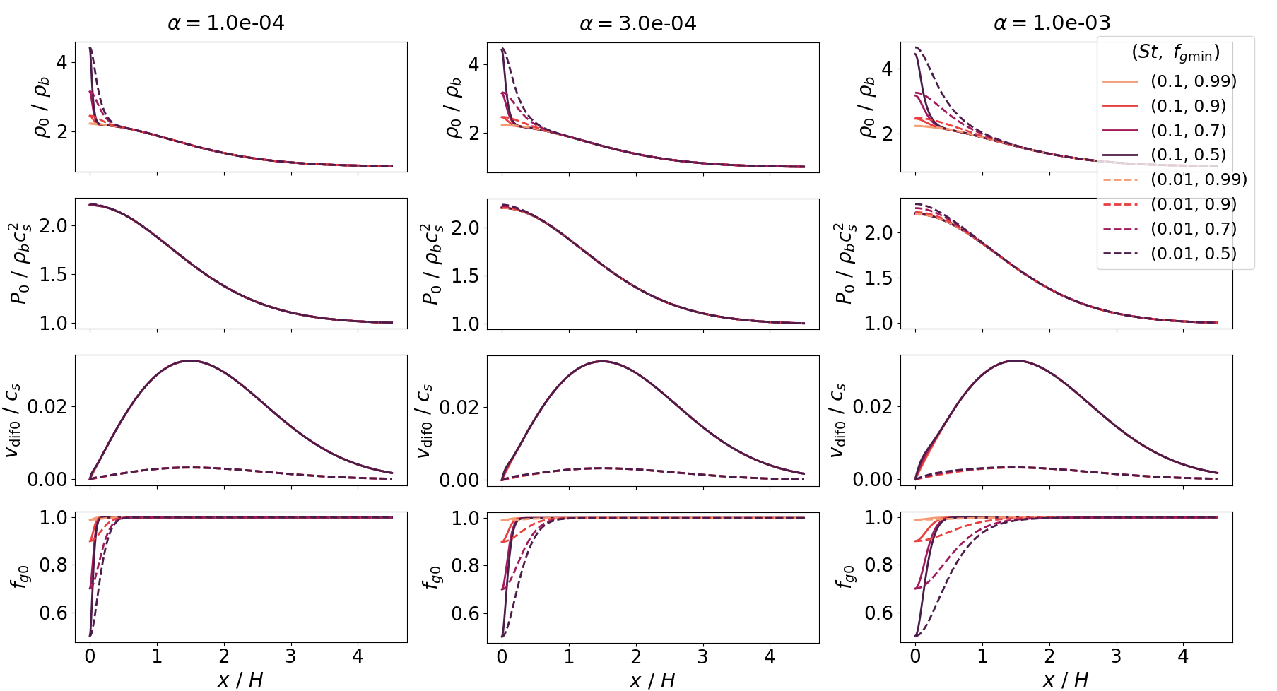
Figure 1: Equilibrium solutions for different combination of parameters. Only the $x>0$ region is plotted; $\rho_{0}$, $P_{0}$ and $f_{g0}$ are even functions in $x$ whereas $v_{\rm dif0}$ is odd. Each row presents $\rho_{0}$, $P_{0}$, $v_{\rm dif0}$ and $f_{g0}$ respectively. For all plots here, $A=0.8$ and $\Delta w/H=1.5$. Three columns correspond to different $\alpha$, as noted on the top. Colors represent different $f_{g{\rm min}}$ while line styles represent different $St$ values.

3.1 Derivation of steady-state equations

In equilibrium, we expect axisymmetry and therefore no dependence on $y$. The radial velocity of the single fluid is also zero: the gas stays at rest, while the bulk velocity of the dust, which drifts towards pressure maxima, is balanced by outward diffusion, giving an overall effect of $\bm{v}^{\prime}_{d0}=0$. The absence of any bulk radial motion reflects the equilibrium state with an isolated dust trap, which is unlike the conventional scenario with dust/gas drifting inward/outward in the presence of a background pressure gradient. Therefore, after separating all vectors into $x$ and $y$ components, we drop the partial derivatives of $t$ and $y$ as well as terms involving $\bm{v}^{\prime}_{0}$ from Equations (20)(21)(22) to obtain

$$v^{\prime}_{0x}=0\ ,$$ (23)

$$c_{s}^{2}t_{s}f_{d0}\frac{\partial P_{0}}{\partial x}+D_{0}P_{0}\frac{\partial\ln f_{g0}}{\partial x}=0\ ,$$ (24)

$$-\frac{1}{\rho_{0}}\frac{\partial P_{0}}{\partial x}+2\Omega_{0}v^{\prime}_{0y}+\frac{1}{\rho_{0}}\frac{\partial}{\partial x}\left[D_{0}^{2}\frac{\rho_{0}^{2}}{\rho_{d0}}\left(\frac{\partial\ln f_{g0}}{\partial x}\right)^{2}\right]=0\ ,$$ (25)

$$\nu f_{g0}\frac{\partial^{2}v^{\prime}_{0y}}{\partial x^{2}}+f_{g0}f_{0}(x)=0\quad\Rightarrow\quad v^{\prime}_{0y}=-\frac{c_{s}^{2}A}{2\Omega_{0}(\Delta w)^{2}}x{\rm e}^{-x^{2}/2(\Delta w)^{2}}\ ,$$ (26)

where we use the fact that $P_{0}(x)$ and $f_{g0}(x)$ have no spatial gradient far from the pressure bump in obtaining Equation (24), which is derived from Equation (22). Note that if there were no forcing, the equilibrium solution would become trivial, where all velocities would vanish and the dust-to-gas ratio would become uniform.

3.2 Numerical solution

We solve the equilibrium equations as an initial value problem by specifying conditions at $x=0$. Due to the symmetry of our setting, $\rho_{0}(x)$ and $P_{0}(x)$ are even functions with respect to $x=0$ and thus we only solve the equations for $x>0$. Our methods are described in detail in Appendix B. We obtain equilibrium solutions with five dimensionless physical parameters, of which the information, fiducial values and the ranges explored in this work are summarised in Table 1.

Among the parameters, $St=0.1$, corresponding to mm- to cm-sized dust for typical disc models in the outer disc, would be an upper bound for our single-fluid formalism to remain approximately valid, which assumes strongly coupled dust and gas. The minimum gas fraction $f_{g{\rm min}}$ is the gas mass fraction at the center of the bump. We choose this parameter rather than a global dust-to-gas ratio by convention because $f_{g{\rm min}}$ is numerically easier to control. Our lower bound of $f_{g{\rm min}}=0.5$ is chosen to correspond to the extreme situation with a $1:1$ gas-to-dust mass ratio in the bump center, which may be the case in some systems such as in HD 142527 (being 1.7, Boehler et al., 2017).

We show in Figure 1 the equilibrium solution in terms of the radial profiles of $P_{0}(x)$, $f_{g0}(x)$ and $v_{\rm dif0}(x)$ for a bump with $A=0.8$ and $\Delta w/H=1.5$. In all combination of parameters below, the density and pressure form a bump close to $x=0$ and quickly approaches the background value as $x$ exceeds $\Delta w$. The density excess close to $x=0$ and the minimum in the gas fraction profile indicate significant increase of dust concentration at the pressure maximum. We call this region a "dust bump" as opposed to the wider gas bump. As can be seen from either $\rho_{0}$ or $f_{g0}$, the width of the equilibrium dust bump depends heavily on $St$ and $\alpha$: the dust bump is considerably narrower than the gas bump if the gas and dust are not well-coupled and/or if the concentration diffusion that balances the dust drift is weak. Tightly coupled systems give a slightly higher maximal pressure, which reflects the dust feedback to the gas.

It is of interest to translate $f_{g{\rm min}}$ to an averaged gas fraction through a ring. We define the mean gas and dust mass fraction $\overline{f_{g}}$ and $\overline{f_{d}}$ as

$$\overline{f_{g}}=1-\overline{f_{d}}=\frac{\int_{-x_{B}}^{x_{B}}P(x)dx}{c_{s}^{2}\int_{-x_{B}}^{x_{B}}\rho(x)dx}\ ,$$ (27)

where $x_{B}$ specifies the radial range of interest. A minimum gas fraction of 0.7 in our fiducial setting corresponds to $\overline{f_{g}}=0.980$ integrated from $x/\Delta w=-4$ to $+4$. In other words, if a bump quasi-statically evolved from a uniform mixture of gas and dust with $\overline{f_{g}}=0.98$ ($\overline{f_{d}}=0.02$), which is a reasonable condition, and if the bump could attract all the dust in a range of $\pm 4\Delta w=\pm 6H$, the equilibrium $f_{g{\rm min}}$ would be equal to our fiducial value. For $f_{g\rm min}=0.7$, a combination of large dust particles and low viscosity ($St=0.1,\alpha=3\times 10^{-5}$) gives $\overline{f_{g}}=0.996$, while $St=0.003,\alpha=1\times 10^{-3}$ gives a rather low $\overline{f_{g}}=0.89$ (we find no “interesting” instability anyway with this configuration or a more realistic $\overline{f_{g}}$). More values of $\overline{f_{g}}$ are annotated later in Figures 7, 8 with notes in Section 5.3.

Parameter	Symbol	Fiducial Val.	Range
Gas bump magnitude	$A$	1.2	0.4–1.8
Gas bump width	$\Delta w/H$	1.5	1.0–2.0
Stokes number	$St$	0.03	0.003–0.1
Viscous parameter	$\alpha$	$3\times 10^{-4}$	$3\times 10^{-5}$–$1\times 10^{-3}$
Minimum gas fraction	$f_{g{\rm min}}$	0.7	0.5–0.99

Table 1: Parameters of the dust-trapping ring.

4 Formulation of the perturbation equations

4.1 Linearised system of equations

Based on the equilibrium results, now we proceed to obtain the perturbation equations to investigate potential instabilities. Using the subscript “₁" to denote perturbation variables, we consider a plane wave perturbation of the form

$$\rho_{1}(x,y,t)={\rm Re}[\rho_{1}(x){\rm e}^{i(ky-\omega t)}]\ ,$$

$$P_{1}(x,y,t)={\rm Re}[P_{1}(x){\rm e}^{i(ky-\omega t)}]\ ,$$

$$\bm{v}_{1}(x,y,t)={\rm Re}[\bm{v}_{1}(x){\rm e}^{i(ky-\omega t)}]\ ,$$ (28)

where $k$ (being a real number) is the $y$-direction wavenumber, $\omega$ is the complex frequency, $i^{2}=-1$, and Re[$\cdot$] takes the real part. The perturbation variables $\rho_{1}(x)$, $P_{1}(x)$ and $\bm{v}_{1}(x)$ throughout this paper represent the complex 1D functions on the right hand side in Equation (28) unless otherwise stated to denote the real 2D waveform. Note that we do not impose (anti-)symmetry here but solve the perturbation equations over the full domain of $x$. The real part of $\omega$ represents oscillation and the imaginary part implies temporal growth or damping in the perturbation magnitude. We write $\omega=\omega_{r}+i\gamma$, where $\omega_{r}$ and $\gamma$ are real. An unstable perturbation with its magnitude growing with time has $\gamma>0$.

We introduce the following notation of perturbation ratios $\mathfrak{p}_{1}(x)\equiv P_{1}(x)/P_{0}(x)$ and $\mathfrak{f}_{g1}(x)\equiv f_{g1}(x)/f_{g0}(x)$. We substitute the perturbations into Equations (13)(20)(21)(22) to obtain the linearised system of equations. The derivation and detailed form of the system are lengthy and involve considerable algebra, which we outline in Appendix A.1. We only show the compact form here, expressed as a matrix of linear operators acting on the perturbation variables:

$$\begin{bmatrix}\mathcal{M}_{00}&\mathcal{M}_{01}&\mathcal{M}_{02}&\mathcal{M}_{03}\\ \mathcal{M}_{10}&\mathcal{M}_{11}&\mathcal{M}_{12}&\mathcal{M}_{13}\\ \mathcal{M}_{20}&\mathcal{M}_{21}&\mathcal{M}_{22}&\mathcal{M}_{23}\\ \mathcal{M}_{30}&\mathcal{M}_{31}&\mathcal{M}_{32}&\mathcal{M}_{33}\end{bmatrix}\begin{bmatrix}\mathfrak{p}_{1}(x)\\ \mathfrak{f}_{g1}(x)\\ v^{\prime}_{1x}(x)\\ v^{\prime}_{1y}(x)\end{bmatrix}=0\ .$$ (29)

This is a system of four second-order linear ordinary differential equations in four functional variables, $\mathfrak{p}_{1}(x)$, $\mathfrak{f}_{g1}(x)$, $v^{\prime}_{1x}(x)$, and $v^{\prime}_{1y}(x)$. The matrix $\mathcal{M}(x,\omega,k)$ consists of block coefficients $\mathcal{M}_{ij}(i,j=0,1,2,3)$, which are differential operators of order at most two and may be functions of $x$, the already known equilibrium variables, and the yet-undetermined perturbation parameters $\omega$ and $k$. For a given $k$, we view the system of equations as an eigenproblem and solve for the eigenvalue $\omega=\omega_{m}$ with the corresponding eigenfunction. The system allows for numerous modes, but only a handful of modes are unstable, which we will focus on.

4.2 Boundary conditions

Boundary conditions are required for a complete eigenproblem. As can be observed from Figure 1, $\rho_{0},P_{0}$ and $f_{g0}$ quickly approach background values as $|x|$ increases, while $v_{\rm dif0}$ shows a slower decay. Therefore, we set $\rho_{0}=\rho_{b},P_{0}=P_{b}=c_{s}^{2}\rho_{b},f_{g0}=1$, and $v^{\prime}_{0y}=0$ at the boundary, while still using nonzero $v_{{\rm dif}0x}(x)$ from the equilibrium solution. Since dust is depleted here, $\mathfrak{f}_{g1}=0$. The perturbation equations at the boundary $x=\pm x_{B}$ can therefore be reduced to three equations in three variables $\mathfrak{p}_{1}$, $v^{\prime}_{1x}$, and $v^{\prime}_{1y}$ (the second perturbation equation becomes trivial).

Now, we apply the WKBJ approximation, i.e., to take $\mathfrak{p}_{1},v^{\prime}_{1x},$ and $v^{\prime}_{1y}$ as a plane wave proportional to $\exp{(ik_{x}x)}$, where $k_{x}$, the asymptotic radial wavenumber shared by the three perturbation variables, is yet to be determined. This form is motivated by the fact that physical quantities in equilibrium vary slowly with $x$ near the boundaries; similar methods have been used by Li et al. (2000); Ono et al. (2016). We stress that $k_{x}$ is only used to specify the asymptotic relation at the boundaries, i.e., we do not assume that the perturbation variables constitute a plane wave everywhere. The boundary perturbation equations are therefore reduced to a linear system, whose coefficient matrix must have a vanishing determinant for a nontrivial solution. The boundary perturbation equations before and after the WKBJ approximation, as well as the form of the determinant, can be found in Appendix A.2.

The zero determinant condition yields a dispersion relation $k_{x}=k_{x}(\omega,k,x)$, which is a polynomial equation of fourth degree in $k_{x}$. Two of the four complex solutions unphysically go to infinity both in real and imaginary parts as $\nu\to 0$. Between the remaining two, one and only one has a positive real part if $k$ is not too close to zero. We obtain this root $k_{x}$ numerically at the outer and inner boundaries respectively and adopt it as the outgoing boundary condition: $d\mathfrak{p}_{1}/dx=ik_{x}\mathfrak{p}_{1},d\mathfrak{f}_{g1}/dx=ik_{x}\mathfrak{f}_{g1},dv^{\prime}_{1x}/dx=ik_{x}v^{\prime}_{1x},$ and $dv^{\prime}_{1y}/dx=ik_{x}v^{\prime}_{1y}$.

4.3 Numerical treatment

We solve the eigenproblem numerically by discretising the differential equations in $x$ and representing all coefficients with matrix elements, similar to Ono et al. (2016). We perform calculations over a range of $-4\Delta w<x<4\Delta w$, which sufficiently covers the pressure bump region, over a uniform grid of $N=1001$ nodes. Doubling the node number would give eigenvalues that agree with our fiducial resolution within three to four digits. To construct the matrix, we use findiff (Baer, 2018), a Python package for finite difference numerical derivatives and partial differential equations in any number of dimensions. We then solve $\omega$ with a positive imaginary part such that the determinant of the matrix goes to zero. Once the desired eigenvalue $\omega_{m}=\omega_{rm}+i\gamma_{m}$ is found, we substitute it for $\omega$ in the matrix and calculate the eigenfunction, which we denote as a vector function in $x$ with parameter $\omega=\omega_{m}$, namely, $\vec{u}_{1m}(x,\omega_{m})=(\mathfrak{p}_{1m}(x),\mathfrak{f}_{g1m}(x),v^{\prime}_{1xm}(x),v^{\prime}_{1ym}(x))^{\top}|_{\omega=\omega_{m}}$. We use the subscript “_m” to denote eigenmodal quantities. We normalise the eigenfunction in magnitude and phase such that $\vec{u}_{1m}(x,\omega_{m})$ has length unity and $\mathfrak{p}_{1m}(0)|_{\omega=\omega_{m}}$ is real. The original perturbation variables $P_{1m}(x)$ and $f_{g1m}(x)$ are then recovered from $\mathfrak{p}_{1m}(x)$ and $\mathfrak{f}_{g1m}(x)$. Finally, the physically meaningful waveform in 2D, as later displayed in Figures 3–5, is obtained from Equation (28), where we arbitrarily take $t=0$. The phases of these 2D waveforms depend on both $x$ and $y$ as the 1D perturbation variables are complex. We describe details of matrix construction and determination of $\omega_{m}$ and $\vec{u}_{1m}(x,\omega_{m})$ in Appendix C.

5 Results of the linear analysis

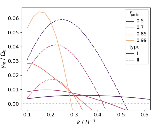
Figure 2: Dispersion relation of a sharp bump, showing $\gamma_{m}$ as a function of $k$, for different dust content measured in $f_{g\rm min}$. Two types of DRWI are plotted using solid and dashed lines respectively. The Type II curve for $f_{g{\rm min}}=0.99$ is below the lower limit of this figure. Parameters are set as $A=1.2$, $\Delta w/H=1.5$, $St=0.03$, $\alpha=3\times 10^{-4}$. The value of $\overline{f_{d}}$ corresponding to each level of $f_{g\rm min}$ is measured as $0.038,0.020,0.009,$ and $6\times 10^{-4}$ respectively.

We identify solutions of the eigenproblem by a broad search on the $\gamma$–$\omega_{r}$ plane (Appendix C). Only two modes are unstable among the numerous solutions. We term them the Type I and Type II DRWI. For reasons to be discussed below, we believe that Type I is a direct generalisation from the classical RWI, whereas Type II is first identified in this work whose origin is closely related to the presence of dust.

The two types are distinguished by the value of $\omega_{rm}$. Type I features $\omega_{rm}=0$, i.e., the mode has no phase velocity at $x=0$ in the rotating frame and therefore is stationary at the pressure maximum. Its eigenfunctions are symmetric or antisymmetric about $x=0$. In contrast, Type II has nonzero $\omega_{rm}$, indicating a co-rotation radius off the peak, and the perturbation profiles do not have the (anti-)symmetry as Type I does.

5.1 Two types of the DRWI: dispersion relation and eigenmodes

Figure 3: Eigenfunctions of Type I DRWI for a system with low dust content ($f_{g{\rm min}}=0.99$). The top panels present the $y$-independent equilibrium profiles $P_{0}$, $\rho_{0}$, and $q_{0}$, and the bottom panels show the perturbation functions $P_{1}$, $\rho_{1}$, and $q_{1}$ respectively. The eigenfunctions are drawn for one and half a wavelength in the $y$-axis, indicated by the phase. Arrows in the bottom panels denotes the perturbed velocity field $\bm{v}^{\prime}_{1}$, with the arrow length proportional to the perturbed speed magnitude. In all panels, a grey dashed line marks the $x$-location of the co-rotation radius. Here $k=0.2H^{-1}$ and $\omega_{m}=(0+0.0577i)\Omega_{0}$ and other parameters are the same as Figure 2.

Figure 4: Eigenfunction of Type I DRWI for a system with moderate dust content ($f_{g{\rm min}}=0.7$). Here $k=0.2H^{-1}$ and $\omega_{m}=(0+0.0096i)\Omega_{0}$. Other details are the same as Figure 3.

Figure 5: Eigenfunction of Type II DRWI for a system with moderate dust content ($f_{g{\rm min}}=0.7$). Here $k=0.2H^{-1}$ and $\omega_{m}=(0.1244+0.0407i)\Omega_{0}$. Other details are the same as Figure 3.

Now, for the purpose of illustration, we demonstrate the main properties of the two DRWI types by a representative result in Figure 2. With fiducial settings of $A=1.2,\Delta w/H=1.5,St=0.03,$ and $\alpha=3\times 10^{-4}$, various values of $f_{g\rm min}=0.5,0.7,0.85,0.99$ are chosen, with the corresponding $\overline{f_{d}}$ measured to be $0.038,0.020,0.009,$ and $6\times 10^{-4}$. Our calculation starts from $k=0.1$, which corresponds to a wavelength of the disc circumference if the local pressure scale height satisfies $H/R_{0}=0.1$. We see that as dust concentration increases, the dispersion relation for the type I DRWI extends to larger $k$ (shorter wavelength), while the fastest growth rates decreases. On the other hand, the fastest growth rate of type II DRWI increases with dust concentration.

In the next, we show the eigenfunctions of the two modes to further examine the underlying physics. Apart from $P_{1},f_{g1},v^{\prime}_{1x},$ and $v^{\prime}_{1y}$, the vortensity $q$ is known to be vital for the mechanism of the RWI and also of interest here. The vortensity is defined by

$$q\equiv\frac{(2-3/2)\Omega_{0}+(\nabla\times\bm{v}^{\prime})_{z}}{\rho}=\frac{1}{\rho}\left(\frac{1}{2}\Omega_{0}+\frac{\partial v^{\prime}_{y}}{\partial x}-\frac{\partial v^{\prime}_{x}}{\partial y}\right)$$ (30)

as proper for pure gas in a Keplerian-rotating shearing sheet (see Appendix A.3). Its linear perturbation is then

$$q_{1}=-\frac{1}{\rho_{0}^{2}}\left(\frac{1}{2}\Omega_{0}+\frac{dv^{\prime}_{0y}}{dx}\right)\rho_{1}+\frac{1}{\rho_{0}}\left(\frac{dv^{\prime}_{1y}}{dx}-ikv^{\prime}_{1x}\right)\ .$$ (31)

Starting from the Type I DRWI, we first look at the case with $f_{g{\rm min}}=0.99$, which is close to the dust-free scenario, and the corresponding eigenfunctions of perturbed pressure, density and vortensity are shown in Figure 3. In this limit, Type I is strongly unstable with a maximal $\gamma_{m}$ on the order of $10^{-2}$ to $10^{-1}\Omega_{0}$, in agreement with the RWI investigated in Ono et al. (2016) with similar gas bump profiles. The pressure and density perturbations show alternate peaks and troughs along the $\hat{y}$ direction accompanied respectively by anti-cyclonic and cyclonic velocity perturbations. The vortensity perturbations show patterns of two Rossby waves along $\hat{y}$ on the two sides of the background vortensity minimum ($x=0$), with a phase difference. The growth of this instability, as explained in Ono et al. (2016), can be ascribed to $v^{\prime}_{1x}$ advecting large background vortensity towards a positive vortensity perturbation and vice versa (e.g., along the horizontal line of phase $0.5\pi$ in Figure 3). On the other hand, for a higher $k$ such that $\gamma_{m}<0$, the vortensity begins to show an opposite phase difference that suppresses the perturbation. Based on these reasons, we recognise Type I as the RWI loaded with dust.

In the eigenfunction described above, the magnitude of the density perturbation is strongly enhanced within the dust bump. The phenomenon becomes more pronounced for a system with higher total dust content. In Figure 4 where $f_{g\rm min}=0.7$ or $\overline{f_{d}}=0.020$, both the density and the vortensity perturbations are mainly concentrated in the dust bump. Vortensity sources are no longer negligible here, while the pattern remains similar to the $f_{g\rm min}=0.99$ case outside the dust bump, where the vortensity-flow explanation of the instability still applies. We will further discuss the instability mechanism in Section 5.4.

The Type II DRWI shows essentially different eigenfunctions (Figure 5). The non-zero $\omega_{rm}$ implies a $y$-direction phase velocity in the co-rotating frame at $x=0$. Therefore, the patterns in Figure 5, where $\omega_{rm}>0$, should be understood as travelling up along the $y$-axis with time. Another viewpoint is that the co-rotation radius $x_{c}$, defined implicitly by $v_{0y}(x_{c})=v^{\prime}_{0y}(x_{c})-(3/2)\Omega_{0}x_{c}=\omega_{rm}/k$, deviates from the pressure maximum towards approximately the edge of the dust bump. For $\omega_{rm}>0$, we have $x_{c}<0$. The pressure perturbation appears distorted across $x_{c}$ and reaches maximum/minimum at $x<0$. The density perturbation forms periodic patterns along $\hat{y}$, with a positive patch on one side of $x=0$ matched with negative on the other side and vice versa. The perturbed vortensity patterns outside the dust bump still resemble two Rossby waves, but now the vortensity advection does not effectively contribute to the growth of the instability in the interval $x_{c}<x<0$. We will elaborate on this observation quantitatively in Section 5.4, where we point out that the Type II DRWI requires vortensity sources in the dust bump to be unstable at all.

As expected from the symmetry of our formulation, Type II DRWI modes always come in pairs: if $\omega_{rm}+i\gamma_{m}$ is an eigenvalue, then so is $-\omega_{rm}+i\gamma_{m}$. The 2D waveform of $-\omega_{rm}+i\gamma_{m}$ can be obtained from that of $\omega_{rm}+i\gamma_{m}$ by mapping $x\mapsto-x$ and $y\mapsto-y$, i.e., by reflection over the origin. The pair of modes likely coexist in real bumps, which implies a complicated mixture of their travelling patterns. Still, one may expect the $P_{1}$ patterns to appear to travel up along the $\hat{y}$ direction on the inner side of the bump $(x<0)$, where a mode with positive $\omega_{rm}$ has much stronger pressure perturbation than its negative-$\omega_{rm}$ counterpart; the opposite is expected on the outer side $(x>0)$. Our simulation in Section 6.1 confirms this prediction.

While the two types of instabilities follow distinct trends in Figure 2, their relation becomes more complicated where the dust bump is sharper. We observe bifurcation phenomena, where Type II merges into or forks from Type I, which we describe in further detail in Appendix D. While the discussion above on eigenfunction remains valid, the bifurcation implies a smooth transition between the two types of the DRWI and hence between symmetric and asymmetric perturbation patterns in strongly unstable regions of the parameter space.

5.2 Effect of viscosity on the RWI

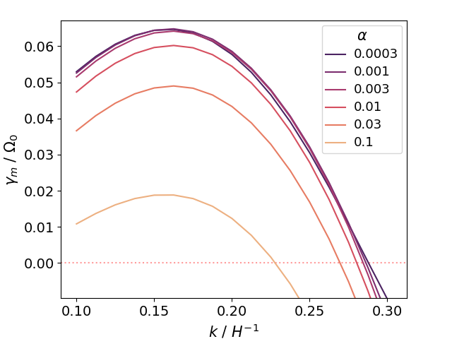
Figure 6: Dispersion relation of the classical RWI with different viscosity. A low gas content of $f_{g\rm min}=0.99$ is considered to approximate the pure-gas limit. Other parameters are set as $A=1.2$, $\Delta w/H=1.5$, $St=0.03$.

We have shown that the dispersion relation and eigenfunction patterns of the Type I DRWI approach those of the classical RWI in the limit of pure gas. However, the DRWI incorporates the turbulent viscosity, a physical process neglected in most previous studies on the RWI. As a short digression, our formulation can naturally be used to calculate the linear behavior of the RWI in the presence of gas turbulence.

In Figure 6, we compare a wide range of $\alpha$ for an approximately dust-free bump ($f_{g{\rm min}}$=0.99). While high viscosity suppresses the instability, $\alpha\leq 3\times 10^{-3}$ hardly influences the dispersion relation. The $y$-direction wavenumber corresponding to the maximal $\gamma_{m}$ also stays almost invariant. Our linear analysis here is consistent with simulations that the RWI in the linear regime is largely unaffected by realistic disc viscosity settings (Lin, 2014). Analytical work by Gholipour & Nejad-Asghar (2014) gave similar results, on which we improve by properly setting up the background equilibrium state.

Figure 7: Grid search of $\gamma_{m*}$ for $f_{g{\rm min}}=0.7$. Each panel is covered by a linearly uniform grid of step size 0.1 along both axes. The values of $St$ and $\alpha$ for each panel are annotated on the axes of the entire figure. Colors represent the value of $\gamma_{m*}$ for a given set of parameters, listed in Table 1, with darker shades denoting higher $\gamma_{m*}$ and white denoting $\gamma_{m*}<0$. In each panel, white dots denote pixels where Type I is more unstable than Type II, the black dotted curve denotes where the dust-free bump is marginally stable to the standard RWI, and the number at the bottom right denotes $\overline{f_{g}}$ averaged over all pixels on the panel. The blue dashed line separates four bottom left panels from the rest, as the former deviate from the trend related to $St$ and $\alpha$ (see discussion in Section 5.3.1). All panels here and in Figure 8 are colored in one single scale for comparison.

Figure 8: Grid search of $\gamma_{m*}$ for $f_{g{\rm min}}=0.5$. This figure is similar to Figure 7. All panels here and in Figure 7 are colored in one single scale for comparison.

Figure 9: Grid search of the most unstable wavenumber $k_{*}$ for $f_{g{\rm min}}=0.7$. Darker shades denote higher $k_{*}$ and white pixels have no unstable mode. We take $k_{*}=0.1H^{-1}$ for monotonically decreasing $\gamma_{m}(k)$ curves. All panels here and in Figure 10 are colored in one single scale for comparison. For other details, see the caption of Figure 7.

Figure 10: Grid search of the most unstable wavenumber $k_{*}$ for $f_{g{\rm min}}=0.5$. This figure is similar to Figure 9. All panels here and in Figure 9 are colored in one single scale for comparison.

5.3 Parameter space of the most unstable DRWI

To understand the parametric dependence of the two types of the DRWI, we perform a grid search in the parameter range listed in Table 1 except that only two levels of dust content, $f_{g{\rm min}}=0.7$ and 0.5, are selected. The maximum growth rates $\gamma_{m*}$ with regard to different $k$ and the corresponding wavenumbers $k_{*}$ are shown in Figures 7, 8 and Figures 9, 10 respectively. For all these figures, each panel represents one particular $(St,\alpha)$, while each pixel in each panel gives one $(A,\Delta w)$. White dots denote pixels where Type I is more unstable than Type II. Black dotted curves denote where the dust-free bump is marginally stable to the standard RWI. We also calculate the mean gas mass fraction $\overline{f_{g}}$ for each pixel. As the bump sharpens, it concentrates dust more vigorously, but the total amount of gas also increases, making $\overline{f_{g}}$ barely dependent on $A$ or $\Delta w$. We show the panel-wise averaged results at the bottom right of each panel, where the significant digits reflect the magnitude of pixel-wise deviation.

5.3.1 Maximum growth rate $\gamma_{m*}$

We first focus on the maximum growth rate (among different $k$). Three levels of inspection reveal the effect of different parameters: between pixels within one panel for $A$ and $\Delta w$, between the sixteen panels within one figure for $St$ and $\alpha$, and between Figures 7 and 8 for $f_{g\rm min}$. In the following, we will start from the first and third levels, where the trends are relatively straightforward, before elaborating on the second level of comparison.

Each panel shows similar pixel-level trends: sharper pressure bumps (large $A$, small $\Delta w$) induce faster growth rates for both types of the DRWI. While the Type I DRWI shows a steep slope with respect to $A$ or $\Delta w$ and prevails for very sharp bumps, Type II dominates in a broad range of realistic parameters and even renders the pressure bump unstable when it is stable to the classical (dust-free) RWI (i.e., colored pixels below the black dotted curve).

Regarding the comparison between Figures 7 and 8, a higher dust concentration tends to stabilise the Type I but destabilise the Type II DRWI, consistent with Section 5.1. For example, the pixel with $St=0.03,\alpha=3\times 10^{-4},A=1.8,\Delta w/H=1.4$ has a darker color in Figure 7 than in Figure 8 (a Type I-dominant case, $\gamma_{m*}=0.16\Omega_{0}$ versus $0.12\Omega_{0}$), whereas the opposite is true for the pixel with $St=0.01,\alpha=1\times 10^{-4},A=0.5,\Delta w/H=1.5$ (Type II-dominant).

Now, we compare different panels within Figure 7 to explain how $\gamma_{m*}$ changes with $St$ and $\alpha$. The comparison also applies to Figure 8. The similar colors on the upper left corner of each panel demonstrate that the Type I DRWI, when dominant, is insensitive to $St$ or $\alpha$. Conversely, the trend of the Type II DRWI is most clearly seen from the lower right region of each panel. For most panels (those above the blue dashed line), a combination of small $\alpha$ and large $St$ shows the broadest range of colored pixels. For example, a bump with $A=0.8$ and $\Delta w/H=2.0$ is unstable to the Type II DRWI for $St=0.03$ and $\alpha=1\times 10^{-4}$, which is not true for $St\leq 0.01,\alpha=1\times 10^{-4}$ or for $St=0.03,\alpha\geq 3\times 10^{-4}$. The total area of colored pixels on the panel $(St,\alpha)=(0.03,1\times 10^{-4})$ or $(0.01,3\times 10^{-5})$ is larger than that on the panel on its upper right, i.e., $(St,\alpha)=(0.03,3\times 10^{-4})$, $(0.01,1\times 10^{-4})$, or $(0.003,3\times 10^{-5})$. In other words, the susceptibility of the system to the Type II DRWI largely varies along the diagonal of the figure from moderately high $St$ and low $\alpha$ (most unstable) to low $St$ and high $\alpha$ (least unstable). We have seen that a sharp pressure bump promotes both types of the DRWI; the correlation here likely similarly points to the Type II DRWI favoring a sharp dust bump in addition to a sharp gas bump (see Figure 1 for how the dust bump profile changes with $St,\alpha$ and $f_{g\rm min}$). Notably, here we believe that $St$ and $\alpha$ only indirectly influence the Type II DRWI by modifying the equilibrium bump profile instead of directly involving in the mechanism of the instability, a point we will argue more rigorously after describing the $k_{*}$ trends.

However, the four panels below the blue dashed line deviate from the diagonal trend as they show a shrinkage of the unstable range compared to adjacent panels on their upper right. This corner corresponds to very low $\alpha$ and relatively large $St$, leading to a very sharp dust bump. We confirm that our resolution is adequate for resolving the dust bump, and speculate on the potential causes that reverse the trend. First, the sharp dust bump implies a very low average dust mass fraction $\overline{f_{d}}$, where dust feedback likely becomes too spatially restricted for the Type II DRWI to operate. Also, weak dust-gas coupling with $St\gtrsim 0.1$ may be subject to two-fluid effects not fully captured in our one-fluid formalism. Later we find that the mechanism of the Type II DRWI does not necessitate streaming motion and thus refrain from further analysis of the marginally coupled system.

5.3.2 Most unstable wavenumber $k_{*}$

We show in Figures 9, 10 the most unstable wavenumber $k_{*}$ in the sense that $\gamma_{m}(k)$ reaches maximum at $k=k_{*}$. The apparent discontinuous transition in $k_{*}$ in most of the panels reflect a switch from Type I (with white dots) to Type II (no white dots) regimes. Generally, for both types of the DRWI, higher maximum growth rates correspond to higher $k_{*}$, as is also seen from Figure 2. For $f_{g\rm min}=0.5$, a few Type I cases have abnormally large $k_{*}$ (e.g., the deep blue pixel at $St=0.003,\alpha=1\times 10^{-4},A=1.0,\Delta w/H=1.1$). This is related to the fact that $\gamma_{m}(k)$ is quite flat in the full dispersion relation of Type I DRWI when $\gamma_{m*}$ is low (cf. Figure 2) and thus $k_{*}$ can be parameter-sensitive. Interestingly, typical unstable wavelengths in $\hat{y}$ are comparable to the disc size and much longer than typical length scales of the SI, the latter being only a fraction of the disc scale height. We find no unstable mode in high $k\gtrsim 1H^{-1}$ (Appendix C), except when we reduce the turbulence level to $\alpha<10^{-6}$. This is likely due to the turbulent diffusion that strongly suppresses small-scale instabilities.

Also, we find that the most unstable wavenumber of the Type II DRWI is insensitive to $St$. The important implication is that this instability is unlikely related to the dust streaming motion, the mechanism used to explain the SI and more generally the resonant drag instabilities (RDI; Squire & Hopkins, 2018), where the outcome sensitively depends on the Stokes number. To further verify this, we conducted another series of calculations, gradually reducing $St$ and $\alpha$ simultaneously until $St\sim 10^{-5}$ and $\alpha\sim 10^{-7}$, so that the dust bump remains similar to that in our fiducial setting (Table 1) but the dust is tightly coupled with the gas. We find that the dispersion relation remains similar for $k\lesssim 1H^{-1}$, pointing to the fact that it is mainly the dust mass loading, rather than dust-gas streaming that shape the properties of this instability. This conclusion is further strengthened by examining the perturbed relative kinetic energy of the dust and the gas with regard to the center of mass (Appendix A.4). In the fiducial eigenfunction with $k=0.2H^{-1}$, it is found to be only 0.06% of the perturbed kinetic energy of the single fluid. The finding sets the stage for our understanding of the Type II DRWI as tightly coupled motion of gas and dust in the following section.

5.4 Physical ingredients of the DRWI

We have identified Rossby waves in the morphology of both types of the DRWI. A Rossby wave is characterised by periodic votensity perturbation patterns with a background vortensity gradient normal to its travelling direction. The vortensity perturbations imply velocity perturbations and hence vortensity advection along the gradient, which solely governs the vortensity budget if the vortensity is conserved (e.g., pure isotropic gas). The RWI, then, is a result of two Rossby waves on each side of a background vortensity minimum positively feeding back to each other (for a detailed interpretation of the Rossby wave and the RWI, see Ono et al., 2016).

The physical picture behind the Rossby waves requires conservation of the vortensity. However, the dust bump introduces vortensity sources, which modifies the RWI to become the Type I DRWI and brings the Type II DRWI into existence. In the following, we analyse the vortensity budget in the dust-trapping ring in Section 5.4.1, which is followed by a discussion in Section 5.4.2 on the evolution of vortensity in and outside the dust bump and the properties of vortensity sources. We aim at identifying the governing physical ingredients of the DRWI, where we demonstrate that the Rossby waves still play important roles in both types of the DRWI, with dust playing a damping/driving role in Type I/Type II. We further tentatively explain in Appendix E the propagation process of the Type II DRWI, but a comprehensive investigation of the instability mechanism is beyond the scope of this paper.

Figure 11: Terms related to the evolution of vortensity of Type II DRWI for a system with moderate dust content ($f_{g{\rm min}}=0.7$). The eigenmode is identical to that shown in Figure 5. The three panels show the time derivative, the baroclinic source, and the advection term of the vortensity perturbation. All panels are colored in one single scale for comparison. The $y$ range, the perturbed velocity field and the co-rotation radius are similarly plotted as in Figure 3.

5.4.1 The vortensity budget

The DRWI involves a mixture of gas and dust that violates the conservation of vortensity. Specifically, the vortensity equation derived from Equations (20)(21) takes the following form:

$$\left(\frac{\partial}{\partial t}+\bm{v}^{\prime}\cdot\nabla-\frac{3}{2}\Omega_{0}x\frac{\partial}{\partial y}\right)q=S\ ,$$ (32)

where the source $S$ satisfies

$$S{\bm{e}}_{z}=\frac{1}{\rho}\nabla P\times\nabla\left(\frac{1}{\rho}\right)+\nu\frac{1}{\rho}\nabla\times(f_{g}\nabla^{2}\bm{v}^{\prime})+$$

$$\frac{1}{\rho}\nabla\times\left[\frac{1}{\rho}\nabla\cdot(\rho_{d}\bm{v}_{\rm dif}\bm{v}_{\rm dif})\right]+\frac{1}{\rho}\frac{\partial[f_{g}f_{0}(x)]}{\partial x}{\bm{e}}_{z}\ .$$ (33)

Derivation of Equation (32) can be found in Appendix A.3. The first term on the right-hand side of Equation (33) is usually known as the “baroclinic" term that arises when the fluid is not barotopic ($\rho$ being only a function of $P$). In our system, the dependence of $\rho$ on $f_{g}$ implies that vortensity may be created or consumed by any misalignment between the density and pressure gradients. The second and third terms might be crudely understood as vortensity diffusion due to gas viscosity and dust concentration diffusion respectively, and the fourth term emerges from the external forcing.

The source terms have zero net contribution in equilibrium: the baroclinic and dust diffusion terms vanish, while the gas diffusion term is balanced by the external torque. In perturbation, though, the vortensity equation will become

$$(-i\omega+ikv^{\prime}_{0y}-\frac{3}{2}ik\Omega_{0}x)q_{1}+\frac{dq_{0}}{dx}v^{\prime}_{1x}=S_{1}=S_{\rm bar1}+S_{\nu 1}+S_{\rm dif1}+S_{\rm ext1}\ ,$$ (34)

where we express the perturbed source as a sum of the baroclinic $S_{\rm bar1}$, viscous $S_{\nu 1}$, dust diffusion $S_{\rm dif1}$, and external forcing $S_{\rm ext1}$ terms, in parallel with the four in Equation (33). In particular,

$$S_{\rm bar1}=\frac{ik}{\rho_{0}^{3}}\left(\frac{d\rho_{0}}{dx}P_{1}-\frac{dP_{0}}{dx}\rho_{1}\right)=-\frac{ikP_{0}v_{{\rm dif}0x}}{\rho_{0}^{2}}\left(\frac{1}{c_{s}^{2}t_{s}}\mathfrak{f}_{g1}+\frac{f_{d0}}{D_{0}}\mathfrak{p}_{1}\right)\ .$$ (35)

This term is dominant among the sources and plays significant roles in the two types of the DRWI, as shown in the following sub-subsection.

5.4.2 Vortensity analysis

We first analyse the vortensity budget of the Type II DRWI, shown in Figure 11. Here, we compare the time derivative of the vortensity perturbation, $-i\omega q_{1}$, the baroclinic source, $S_{\rm bar1}$, and the advection term, $-[ikv^{\prime}_{0y}-(3/2)ik\Omega_{0}x]q_{1}-(dq_{0}/dx)v^{\prime}_{1x}$. We find that the combination of the middle and right panels in Figure 11, representing the latter two terms, largely account for the total vortensity perturbation, as shown in the left panel. We have also examined that the contributions from other terms, primarily from gas and dust diffusion, are relatively minor and only yield certain small-amplitude fine-scale features.

The baroclinity barely appears in the interval $x<x_{c}$ and is relatively weak in $x>0$. Advection dominates the evolution of $q_{1}$ in these regions, supporting our interpretation of classical Rossby waves based on the conservation of vortensity. However, in the narrow interval in between, $S_{\rm bar1}$ is stronger and one observes a discrepancy between $-i\omega q_{1}$ and the advection. To quantify the effects of the baroclinity and the advection, we select the region $x_{c}\leq x\leq 0,0\leq ky<2\pi$ and calculate the cross-correlation between $q_{1}$ and the three terms shown in Figure 11 along the $y$-axis with circular boundary conditions. The results are all sinusoidal as expected. Measuring the phase of the sinusoids, we find that the time derivative of $q_{1}$ has a phase lead of $71.9^{\circ}$ over $q_{1}$ itself, which is plainly equal to $-{\rm arg}(-i\omega_{m})$. The angle is less than $90^{\circ}$ (a positive imaginary part of $\omega_{m}$), indicating instability. $S_{\rm bar1}$ lags behind $q_{1}$ by $24.3^{\circ}$, a small angle compared to $90^{\circ}$, thus significantly enhancing $q_{1}$. In contrast, the advection term leads $q_{1}$ by $89.7^{\circ}$. The instability in the interval $x_{c}<x<0$, then, may be interpreted as the baroclinic source driving the growth of the vortensity perturbation, whereas the advection only serves to propagate the $q_{1}$ patterns.

We also perform similar calculations on the Type I DRWI exemplified in Figure 4. In the region $-0.3H\leq x\leq 0,0\leq ky<2\pi$ (roughly the left half of the dust bump), the advection is completely in phase with $q_{1}$ whereas the baroclinic source lags behind by $162.2^{\circ}$. Now, the advection encourages the growth of $q_{1}$ even in the dust bump, but the baroclinic source still works against the advection. This explains why the dust tends to suppress the Type I DRWI: the dust saps the perturbed vortensity from the positive feedback loop involving the Rossby waves. In this sense, the same mechanism of instability underlies the Type I DRWI and the classical RWI. This concludes our analysis on the interaction between the dust bump and the gaseous Rossby waves in the linear regime of the DRWIs.

6 Numerical test and the nonlinear regime

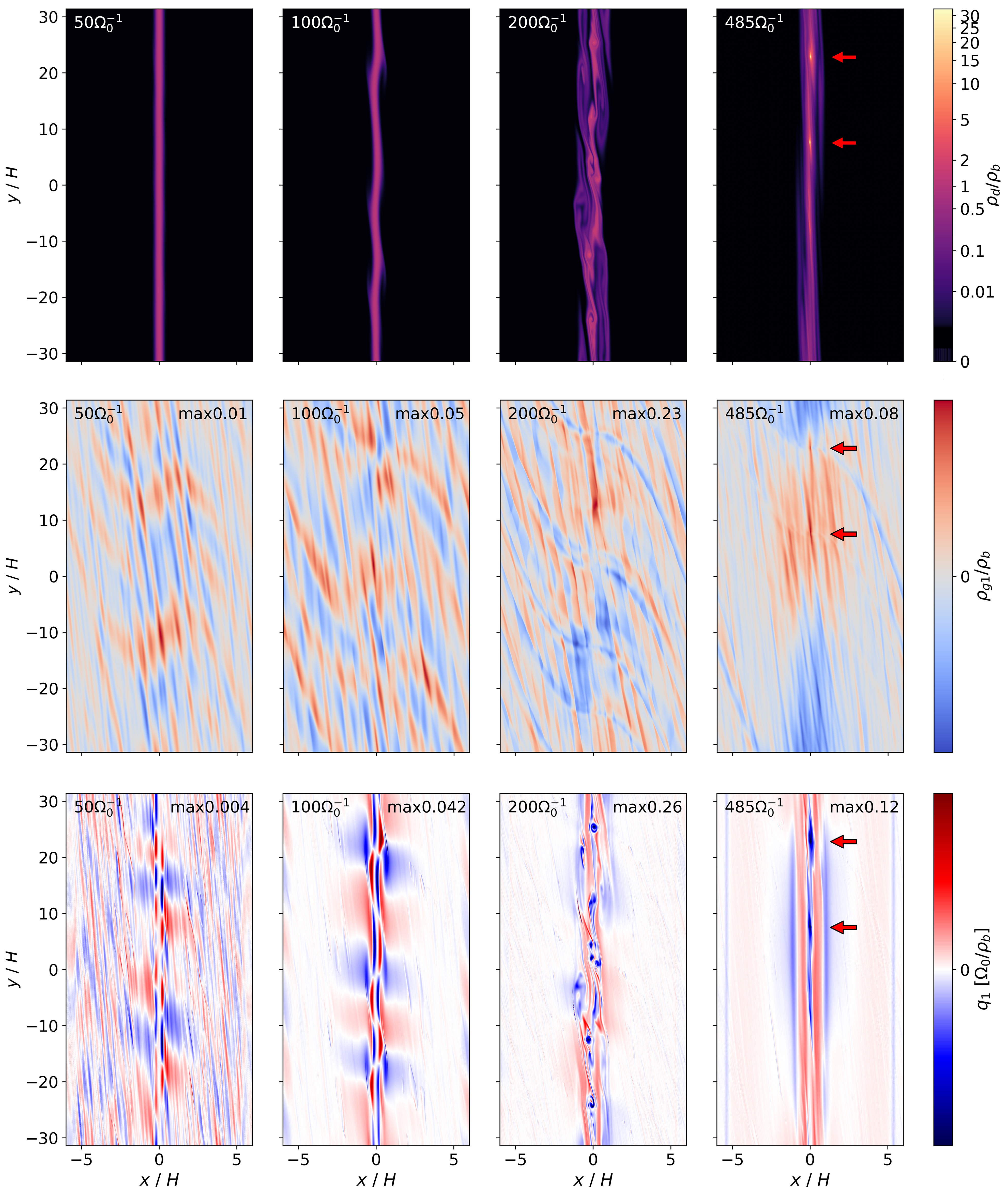
Figure 12: Snapshots in the “mild bump” run of the dust density, perturbed gas density and perturbed one-fluid vortensity (Equation (34)) after inserting the perturbation. Note that the aspect ratio is not drawn to scale. The time is annotated on the top left of each panel. Panels in the top row are colored in the same power-law scale. Panels in the middle and bottom rows are colored linearly and not in the same scale: the maximum $|\rho_{g1}|$ or $|q_{1}|$ of each is annotated on the top right. Red arrows in the last column point to dust density maxima.

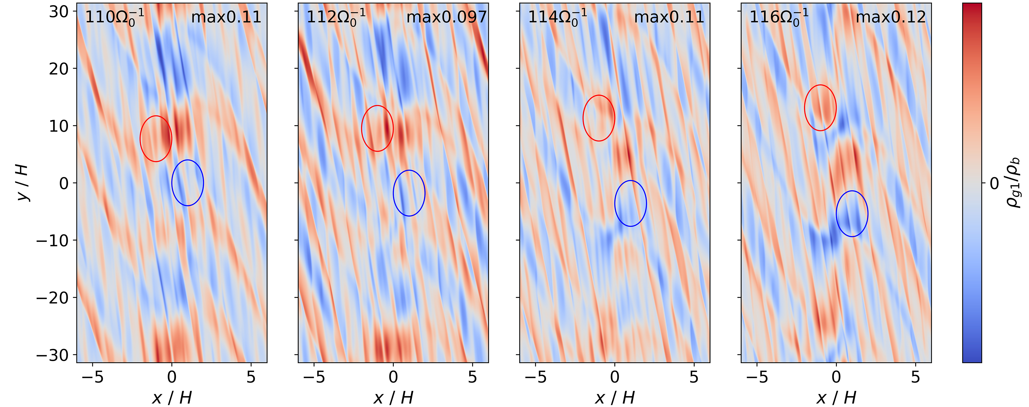
Figure 13: Same as the middle row in Figure 12, but in a shorter time-scale. Red and blue circles ($v_{y}=\pm 0.9c_{s}$) indicate azimuthally travelling patterns.

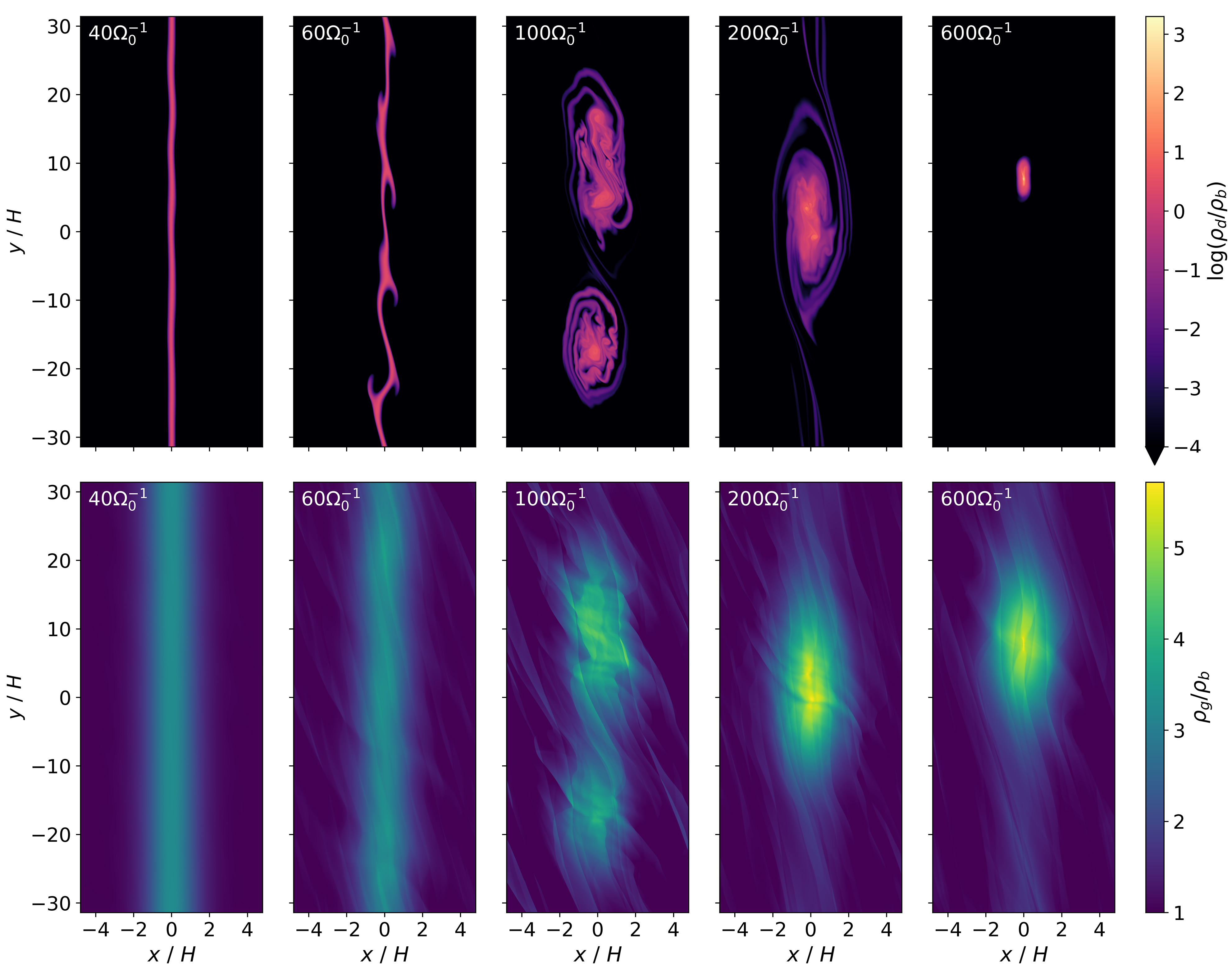
Figure 14: Snapshots in the “sharp bump” run (the Type I DRWI being unstable) of the dust and gas density after inserting the perturbation. The time is annotated on the top left of each panel. The top row is colored in the same logarithmic scale and the bottom in the same linear scale.

In this section, we qualitatively verify the two types of DRWI and investigate their evolution in the nonlinear regime. We use the multifluid dust module in Athena++ (Stone et al., 2008; Huang & Bai, 2022). Our numerical setup keeps the formulation in Section 2.1 and 2.2, treating the gas and dust as two fluids in a local shearing sheet and establishing the external forcing to maintain the pressure bump. Differently, though, we adopt the standard Navier-Stokes viscosity in Athena++. The external forcing is then modified to satisfy the new equilibrium equation in place of Equation (6):

$$f_{0}(x)+\frac{1}{\rho_{g0}}\frac{\partial}{\partial x}\left[\rho_{g0}\nu\frac{\partial}{\partial x}\left(v^{\prime}_{0y}-\frac{3}{2}\Omega_{0}x\right)\right]=0\ ,$$ (36)

which gives the form of $f_{0}(x)$ implemented in the simulation:

$$f_{0}(x)=-\frac{A}{2}\alpha c_{s}\Omega_{0}\left(\frac{H}{\Delta w}\right)^{3}\left(-\frac{x^{3}}{\Delta w^{3}}+\frac{3x}{\Delta w}\right)\exp\left(-\frac{x^{2}}{2\Delta w^{2}}\right)+$$

$$-\frac{A^{2}}{2}\alpha c_{s}\Omega_{0}\left(\frac{H}{\Delta w}\right)^{3}\left(-\frac{x^{3}}{\Delta w^{3}}+\frac{x}{\Delta w}\right)\exp\left(-\frac{x^{2}}{\Delta w^{2}}\right)+$$

$$-\frac{3A}{2}\alpha c_{s}\Omega_{0}\left(\frac{H}{\Delta w}\right)\left(\frac{x}{\Delta w}\right)\exp\left(-\frac{x^{2}}{2\Delta w^{2}}\right)\ .$$ (37)

Also, we use the conventional treatment that includes the dust concentration diffusion in the continuity equation and does not absorb ${\bm{v}}_{\rm dif}$ into ${\bm{v}}_{d}$ (Huang & Bai, 2022, Equation (A1)).

We expect no substantial deviation in terms of linear evolution where viscosity and dust diffusion processes are unimportant. However, the equilibrium profile is slightly influenced by the different setups in the simulation compared to our analytical derivation (mainly due to the use of two-fluid instead of single-fluid formalism), and we reach the steady state by a preliminary axisymmetric run. For a given set of parameters, we use a sheet size of $x\times y=8\Delta w\times 0.078125\pi H$ with $1024\times 12$ cells. Initially, we set $\rho_{g}$ as in Equation (8), $v^{\prime}_{gy}$ and $v^{\prime}_{dy}$ as in Equation (26), and $v^{\prime}_{gx}=v^{\prime}_{dx}=0$. The initial dust density is set as a Gaussian whose height satisfies $f_{g\rm min}$ and whose width ensures that the total dust weight equals to that calculated in Section 3. After the equilibrium is reached, we scale up the simulation with a sheet size of $x\times y=8\Delta w\times 20\pi H$ with $1024\times 3072$ cells, which has the same resolution as the preliminary run and is enough to capture a linear wave of $k=0.1H^{-1}$.

To verify the Type II DRWI, we use the parameter $A=0.8,\Delta w/H=1.5,St=0.03,\alpha=1\times 10^{-4},$ and $\overline{f_{g}}=0.980$ (or equivalently $f_{g\rm min}=0.536$). Our linear calculations predict that this system is stable to the Type I DRWI while $\gamma_{m*}=0.03\Omega_{0}$ for Type II. We preliminarily run this system for 10000 $\Omega_{0}^{-1}$, after which the time derivative of the dust density is below $10^{-6}\rho_{b}\Omega_{0}$. Then, we insert random noise of amplitude $0.01c_{s}$ into the gas velocity and run the full-scale simulation. We term it the “mild bump” run. This run with the dust turned off is tested to be stable to the RWI. We also study a “sharp bump” run where the Type I DRWI dominates. The parameter is $A=1.2,\Delta w/H=1.2,St=0.03,\alpha=1\times 10^{-4},$ and $\overline{f_{g}}=0.980$ (or equivalently $f_{g\rm min}=0.541$), to which our linear calculations predict that $\gamma_{m*}=0.12\Omega_{0}$ and $0.10\Omega_{0}$ for the Type I and II DRWI respectively. This run follows the same procedures as described above. We will describe the two runs separately in the following subsections.

6.1 The mild bump run: development of the Type II DRWI

The evolution of the “mild bump” run ($A=0.8,\Delta w/H=1.5$) is shown in Figure 12 and Figure 13. The dust-gas instability starts to evolve into the nonlinear regime when $t\gtrsim 100\Omega_{0}^{-1}$. Before that, the dominant azimuthal wavenumber is approximately $k=0.3$. The gas and dust density perturbations are anti-correlated. Moreover, Figure 13 shows azimuthally travelling gas density perturbation patterns with $v_{y}\simeq\pm 0.9c_{s}$. These are characteristic of the Type II DRWI. The upward-moving patterns at $x<0$ correspond to the Type II DRWI mode with $\omega_{rm}>0$, while the downward-moving patterns at $x>0$ the mode with $\omega_{rm}<0$.

Upon entering the nonlinear regime after $t\geq 200\Omega_{0}^{-1}$, the dust ring is deformed into anticyclonic vortices, where dust becomes more and more concentrated into scales $\lesssim H$, with maximum $\rho_{d}$ constantly increasing. These dust-gathering vortices correspond to negative one-fluid vortensity perturbation seen in the bottom panels of Figure 12. Interestingly, their locations seem unrelated to the sign of the pressure perturbation: they may stay in either positive or negative pressure extrema or no extremum at all. More precisely, whereas the $\rho_{g1}$ patterns are still travelling at an azimuthal velocity comparable to the sound speed, the dust vortices become almost stationary. Moreover, the gas density perturbation gradually decays in magnitude (compare the maximum $|\rho_{g1}|$ at $t=200\Omega_{0}^{-1}$ and $t=485\Omega_{0}^{-1}$), reaching a characteristic level of $\rho_{g1}/\rho_{b}\lesssim 10\%$, in contrast to the still-concentrating dust vortices. In the meantime, the system is accompanied by numerous fine-scale density waves, presumably triggered by local dust concentrations.

The dust is continuously gathered and dusty vortices merge into each other. Several hundred $\Omega_{0}^{-1}$ after we insert perturbation, one or two dust-loaded vortices are left with maximum dust density $\rho_{d\rm max}/\rho_{b}$ ranging from several tens to more than one hundred. Although this slightly falls short of the density threshold for gravitational collapse (e.g., $\rho_{d\max}/\rho_{b}\gtrsim 200$ in typical outer disc conditions; see Equation (16) and Section 5.1 in Xu & Bai, 2022a), dust vertical settling is not included in this work. The equilibrium dust scale height can be estimated by $H_{d}/H=\sqrt{\alpha/St}=0.06$ (Dubrulle et al., 1995). Under the assumption that the vertical dimension does not impact adversely on dust concentration in 2D, this will suffice to lead to planetesimal formation by clumping even if dust mass loading itself does not further promote settling (which could be observed in 2D axisymmetric and 3D simulations; see Lin, 2019; Xu & Bai, 2022b). Moreover, the dust in each of these vortices is likely massive enough for the self-gravity to overcome turbulent diffusion, for which Klahr & Schreiber (2020) derived a critical minimum dust cloud radius $l_{c}/H=\sqrt{\delta/9St}$, where $\delta\equiv D/c_{s}H$ is the dimensionless diffusivity. In our problem ($\delta<\alpha=1\times 10^{-4},St=0.03$), $l_{c}<0.02H$. In comparison, the typical length scale of the dust vortices at $t=485\Omega_{0}^{-1}$, measured in regions with $\rho_{d}\geq 12\rho_{b}$ (so that the actual dust-to-gas density ratio reaches $\sim 200$ after accounting for dust settling), reaches $\sim 0.06H$ in $x$ and $\sim 0.6H$ in $y$.

The total dust mass in each vortex that is gravitationally bound is estimated as

$$m_{d,\rm vortex}\simeq 0.2\left(\frac{R_{0}}{30{\rm au}}\right)^{2}\left(\frac{H/R_{0}}{0.1}\right)\left(\frac{\rho_{b}}{1\rm g/cm^{2}}\right){\rm M_{\oplus}}\ .$$ (38)

This is larger than the mass of typical planetesimals and may already be considered to be planetary embryos if it collapses into a single object. On the other hand, we caution that our study lacks the vertical dimension and does not include self-gravity, and thus the fate of such dust clumps remains to be revealed. In the absence of self-gravity they are quickly dissipated after several tens of $\Omega_{0}^{-1}$, although they re-emerge $\sim 400\Omega_{0}^{-1}$ later when the dust is spread back into the ring and then triggers a new round of the Type II DRWI. Moreover, the nonlinear outcome of the DRWI also likely depends on the nature of disc turbulence where our treatment is highly simplified. We speculate that the system may instead form multiple planetesimals (as suggested in Xu & Bai, 2022b), especially as there is no strong gas vortex that may tend to gather all nearby dust towards a common collapse site at its center.

One important characteristic of dust clumping in the Type II DRWI is that the dust ring is retained. This is primarily because of the weak density perturbations in the gas (as opposed to the Type I case to be discussed next). As a result, dust concentration may not be easily identified observationally, especially when the dust ring is optically thick. On the other hand, the Type II DRWI does induce certain level of azimuthal asymmetries in the form of non-uniform dust distribution and/or corrugation. For example, in the last column in Figure 12, the large-scale dust mass azimuthal contrast (estimated as the dust density within the most massive quarter of the $y$ range divided by that within its opposite quarter) is $\sim 3$. Azimuthal assymetries in dust rings up to similar levels of contrast have been seen in a number of systems such as DM Tau (Hashimoto et al., 2021) and LkCa 15 (Facchini et al., 2020; Long et al., 2022), and they are suggested to be common (van der Marel et al., 2021). Such azimuthal asymmetries could serve as indirect evidence for the presence of Type II DRWI and hence dust clumping. Our results further suggest that peaks in the azimuthal brightness profile in dust ring are not necessarily co-spatial with the azimuthal gas pressure maxima.

6.2 The sharp bump run: dominance of the Type I DRWI

In the “sharp bump” run ($A=1.2,\Delta w/H=1.2$), shown in Figure 14, we observe that dust and gas vortices develop and merge, forming one single anticyclonic gas vortex at saturated state approximately $200\Omega_{0}^{-1}$ after the initial perturbation. The overall evolution process closely resembles the development of the standard RWI in dusty discs (Meheut et al., 2012; Zhu et al., 2014), and as a result, all the dust in the ring concentrates towards the gas vortex center. This is clearly distinct from the mild bump run where the dust ring is retained thanks to low levels of gas perturbation while developing dust concentration and clumping within the ring. In our sharp bump run, the contraction of the dust in the vortex continues to develop (while the gas vortex has already saturated), eventually saturating at $t\simeq 600\Omega_{0}^{-1}$ with $\rho_{d\rm max}/\rho_{b}\simeq 2\times 10^{3}$. This peak dust density is significantly higher than the Type-II case, and we can also estimate the total dust mass gathered in the vortex to be

$$m_{d,\rm vortex}\simeq 4\pi R_{0}\Delta w\overline{\rho_{d}}=4\left(\frac{R_{0}}{30{\rm au}}\right)^{2}\left(\frac{H/R_{0}}{0.1}\right)\left(\frac{\rho_{b}}{1\rm g/cm^{2}}\right){\rm M_{\oplus}}\ ,$$ (39)

where $\rm M_{\oplus}$ is the Earth mass. This is also much higher than the Type II counterpart, and is in the mass range of planetary embryos. Again, future 3D studies including self-gravity is needed to reveal the fate of such dust clump. Also, we observe that the gas vortex has long lifetimes of at least $1000\Omega_{0}^{-1}$, although the peak dust density fluctuates between $10^{1}\rho_{b}$ and $10^{3}\rho_{b}$ after saturation. The lifetime of dust-laden vortices in 2D has been studied extensively (Chang & Oishi, 2010; Fu et al., 2014b; Crnkovic-Rubsamen et al., 2015; Lovascio et al., 2022) and depends on factors such as the initial dust-to-gas mass ratio, viscosity, dust feedback and dust grain size. The vortex in our sharp bump run is consistent with Lovascio et al. (2022) with similar spatial scale, dust size and total dust-to-gas mass ratio (lifetime $\sim 10^{3}\Omega_{0}^{-1}$ there). Works on planet-induced (Li et al., 2020; Hammer et al., 2021) or 3D (Lyra et al., 2018; Hammer & Lin, 2023) vortices with dust feedback suggested similar longevity, although dust settling could disturb the midplane vortex structure. Since the dust is well confined in the long-lived gas vortex, we speculate that the stronger dust clump resulting from Type I DRWI is more likely to form massive planetesimals/planetary embryos.

One uncertainty in our scenario is that maximum dust density in dusty vortices is very sensitive to the prescription of dust diffusivity $D$, which is currently given as a function of the local dust and gas density. If we assume no weakening of turbulent diffusion due to the dust mass loading, $\rho_{d\rm max}$ will reduce by approximately one order of magnitude for both the mild and sharp bump runs. In previous works, enhanced dust mass loading with dust feedback is found to reduce turbulent diffusion in the magneto-rotational instability (MRI) turbulence (Xu & Bai, 2022b). SI-induced turbulent diffusivity was also found to be sensitive to the dust-to-gas ratio (Schreiber & Klahr, 2018). Further investigations in dust diffusivities within dust clumps are needed that incorporates more realistic background gas turbulence.

7 Summary and discussion

We introduce a physically-motivated local shearing sheetmodel of turbulent dust-trapping rings in PPDs. We establish a pressure bump by implementing a forcing term that mimics torques that drive ring formation (e.g., by planets, or magnetic flux concentration), balanced by viscosity that mimics disc turbulence. The dust is modeled as a fluid including backreaction, which also evolves into an equilibrium dust bump profile by balancing radial drift towards pressure maxima and turbulent diffusion. We aim to identify linear instabilities that operate and potentially lead to planetesimal formation in this realistic setting.

We find two types of instabilities, which we term the DRWI. Type I is generalised from the standard RWI while Type II is first identified here. The Type I DRWI, characterised by a vanishing phase velocity and (anti-)symmetric eigenfunction patterns, dominates in relatively sharp pressure bumps and/or bumps with low dust content. In contrast, the Type II DRWI travels along the $y$ axis, has different perturbation magnitudes on either side of the pressure bump, and operates in relatively mild and dusty bumps. Its maximum growth rate is largely determined by the equilibrium gradients of the gas and dust density.

The standard RWI is understood in terms of conservation of vortensity. However, our vortensity source analysis highlights the effective baroclinity in the dust bump, which only consumes the vortensity budget in the Type I DRWI but mainly contributes to the vortensity growth in Type II. Therefore, we believe that vortensity advection, the incentive of the classical RWI, also accounts for the growth of the Type I DRWI, while both the advection and baroclinity drive the Type II DRWI.

The two types of DRWI are qualitatively verified in simulations, and they show distinct nonlinear outcomes with major observational implications. In general, Type I DRWI dominates in the presence of a sharp bump. This yields a standard gas vortex characterized by a pressure maximum in the center, and it traps and concentrates all the dust originally in the ring. On the other hand, in a mild bump, the Type II DRWI operates and develops into sub-$H$-sized dust anticyclones, whereas the gas density only shows weak perturbations. This allows the dust ring to be largely preserved, while exhibiting azimuthal asymmetries. In both cases, the non-linear evolution of the DRWI triggers significant dust mass loading in the form of dust vortices, which hold potential for dust clumping and hence planetesimal formation or direct formation of planetary embryos.

7.1 Discussion

The DRWIs are likely closely related to certain instability phenomena in previous simulations of pressure bumps with dust feedback. For example, they provide a potential explanation to simulations in Xu & Bai (2022b), where the ring could be broken into dusty non-axisymmetric filaments, qualitatively similar to the nonlinear patterns of the Type II DRWI. Also, at the outer edge of a dead zone, the steep increase of turbulent viscosity leads to radial local gas overdensity. While a sufficiently narrow transition width induces formation of large-scale gas vortices with dust concentrating inside (ascribed to the RWI, Miranda et al., 2017, with the dust content found to impede vortex formation and dust concentration), a smoother transition produces no large-scale gas vortices but dust clumps of scales $\lesssim H$ (Huang et al., 2020). The edge of a gap opened by a massive planet is subject to similar instabilities, with large-scale gas vortices emerging only in the absence of dust backreaction while non-negligible dust concentration instead encourages formation of small dust vortices (Yang & Zhu, 2020). 3D simulations in VSI-turbulent pressure bumps also found a tendency of dusty vortex formation towards axisymmetric rings for increasing average dust-to-gas mass ratio or the Stokes number (Lehmann & Lin, 2022). While further investigation is needed, the Type II DRWI offers a viable physical explanation of these findings.

It is worth considering how our local analyses and simulations of the DRWI fit in realistic global disc structures, which has geometric curvature as well as a background pressure gradient. We expect the instability to be qualitatively robust in the presence of the disc curvature since we recover the classical RWI. Pan & Yu (2020) noted that sustaining Rossby waves requires the presence of the second derivative of the background shear (of order $\Omega_{0}/R_{0}$), which the standard shearing sheet does not capture in background equilibrium. This is resolved as we form a pressure bump that provides strong radial structure ($\partial^{2}v^{\prime}_{0y}/\partial x^{2}\sim\Omega_{0}/H\gg\Omega_{0}/R_{0}$). Further, our physical ingredient analysis suggests that the DRWI is probably insensitive to the particular bump shape with or without a background pressure gradient, as long as the pressure maximum concentrates dust to serve as the vortensity source and the two bump flanks provide equilibrium vortensity slopes. On the other hand, a background pressure gradient can induce a net dust radial flux if no other dust trap exists outside the bump in question. The dust drift could trigger the two-dimensional SI in small scales (Pan & Yu, 2020) that may coexist and/or interact with the DRWI.

The ubiquity of dust-trapping rings and the relatively rarer occurrence of high-contrast asymmetries such as arcs and crescents (Andrews, 2020) suggest that most of the rings are likely moderate in sharpness: they must trap dust effectively in the presence of background radial drift while still stable to the vortex-forming Type I DRWI. This implication is related to the recent global study by Chang et al. (2023), which showed that isothermal axisymetric pressure maxima remain (classical-) RWI-stable for a reasonably large range of bump widths. On the other hand, weak-to-modest level of azimuthal asymmetry in dust rings appears to be common (van der Marel et al., 2021). This is suggestive that the Type II DRWI likely operates and leads to dust clumping while preserving the overall morphology of the dust rings. Another possibility is that dust-laden vortices do form but quickly die out, although the exact lifetime is model-sensitive (e.g., Fu et al., 2014a, b; Rometsch et al., 2021; Hammer & Lin, 2023).

The dust-trapping ring rests in a broader context of spatial and size evolution of solids in PPDs. The Type II DRWI favors relatively large particles with $St=10^{-2}$–$10^{-1}$, consistent with upper bounds of drift-limited dust size in typical conditions in outer PPDs (Birnstiel et al., 2012). The ring is found to further enhance the average dust size by alleviating drift and fragmentation barriers (Li et al., 2019; Laune et al., 2020), thus likely encouraging the onset of the DRWI. It is conceivable that the pressure bump gathers and nurses the dust progressively over drift and coagulation time-scales until mature for the instability.

The formation of planetesimals/embryos in the pressure bump bears on their later evolution paths. For instance, formation models built out of a self-interacting planetesimal ring (regardless of their origin) can be compatible with the formation scenario of terrestrial planets and super-Earths (Woo et al., 2023; Batygin & Morbidelli, 2023). A dust-trapping ring also likely allows pebble accretion to operate efficiently that leads to rapid planet assembly (Jiang & Ormel, 2023). The fact that Type II DRWI leaves the pressure bump largely intact likely favors the production of a planetesimal ring and/or direct formation of embryos which fit into the scenarios above.

Our study bears a number of simplifications and caveats that deserve future studies. Among them includes the local treatment of the isolated pressure bump, as discussed above. Moreover, our 2D study also neglects vital 3D processes such as dust settling and vertical gas flow, which may alter the linear DRWI and its non-linear evolution. We approximate the dust-gas mixture with a single fluid, although two-fluid simulations largely agree with the calculations. Self-gravity is ignored throughout this work, and thus planetesimal/embryo formation is only inferred. Also, our treatment of the MRI turbulence as a diffusive process and of the dust diffusivity as a simplistic function calls for first-principle insights in modelling the MRI and/or other forms of turbulence. We intend to generalise our work to 3D in the future, with a more realistic and thorough consideration of physical processes. Despite current limitations, our work pioneers a rigorous effort to uncover fundamental dynamical scenarios that bridge widespread observed dust structures to the crucial evolutionary stage of solid material towards future planets.

Data Availability

Data of the linear analyses and simulation in this paper are available upon request to the authors.

Appendix A Derivations

A.1 Perturbation equations

To derive the system of perturbation equations (29), we first use the definitions of $f_{d}$, $\bm{v}_{\rm dif}$, $D$ and $\rho$ in Equations (13)(15)(19) to obtain their perturbed forms, also denoted with a subscript $``_{1}"$:

$$f_{d1}=-f_{g0}\mathfrak{f}_{g1}\ ,$$ (40)

$$v_{{\rm dif}1x}=\left(\frac{D_{0}}{f_{d0}}\frac{d}{dx}+\frac{f_{g0}}{f_{d0}}v_{{\rm dif}0x}+\frac{D_{0}^{\prime}f_{g0}v_{{\rm dif}0x}}{D_{0}}\right)\mathfrak{f}_{g1}\ ,$$ (41)

$$v_{{\rm dif}1y}=\frac{ikD_{0}}{f_{d0}}\mathfrak{f}_{g1}\ ,$$ (42)

$$D_{1}=D^{\prime}_{0}f_{g0}\mathfrak{f}_{g1}\ ,$$ (43)

$$\frac{\rho_{1}}{\rho_{0}}=\mathfrak{p}_{1}-\mathfrak{f}_{g1}\ ,$$ (44)

where $D_{0}^{\prime}\equiv[dD(f_{g})/df_{g}]_{f_{g}=f_{g0}}$.

We will heavily use equilibrium solutions in the detailed form of the perturbation equations. We avoid explicitly using $x$-derivatives of $P_{0}$, $f_{g0}$ and $\rho_{0}$ to circumvent numerical errors, instead substituting them with $v_{{\rm dif}0x}$:

$$\frac{1}{P_{0}}\frac{dP_{0}}{dx}=-\frac{v_{{\rm dif}0x}}{c_{s}^{2}t_{s}}\ ,$$ (45)

$$\frac{1}{f_{g0}}\frac{df_{g0}}{dx}=\frac{f_{d0}v_{{\rm dif}0x}}{D_{0}}\ ,$$ (46)

$$\frac{1}{\rho_{0}}\frac{d\rho_{0}}{dx}=-(\frac{1}{c_{s}^{2}t_{s}}+\frac{f_{d0}}{D_{0}})v_{{\rm dif}0x}\ .$$ (47)

These representations come from Equations (13)(19)(24).

The next step is to linearise the single fluid equations. Substitution of the perturbation variables into Equations (20)(21)(22) gives

$$-i\omega\rho_{1}+\frac{d(\rho_{0}v^{\prime}_{1x})}{dx}+ik(v^{\prime}_{0y}\rho_{1}+\rho_{0}v^{\prime}_{1y}-\frac{3}{2}\Omega_{0}x\rho_{1})=0\ ,$$ (48)

$$-i\omega P_{1}+\frac{d(P_{0}v^{\prime}_{1x})}{dx}+ik(v^{\prime}_{0y}P_{1}+P_{0}v^{\prime}_{1y}-\frac{3}{2}\Omega_{0}xP_{1})=$$

$$c_{s}^{2}t_{s}\frac{d}{dx}\left(f_{d0}\frac{dP_{1}}{dx}\right)-c_{s}^{2}t_{s}k^{2}f_{d0}P_{1}+c_{s}^{2}t_{s}\frac{d}{dx}\left(\frac{dP_{0}}{dx}f_{d1}\right)+\frac{d(f_{d0}P_{0}v_{{\rm dif}1x})}{dx}+$$

$$ikf_{d0}P_{0}v^{\prime}_{{\rm dif}1y}+\frac{d(f_{d1}P_{0}v_{{\rm dif}0x})}{dx}+\frac{d(f_{d0}P_{1}v_{{\rm dif}0x})}{dx}\ ,$$ (49)

$$-i\omega v^{\prime}_{1x}+v^{\prime}_{0y}ikv^{\prime}_{1x}-\frac{3}{2}ik\Omega_{0}xv^{\prime}_{1x}=-\frac{1}{\rho_{0}}\frac{dP_{1}}{dx}+\frac{\rho_{1}}{\rho_{0}^{2}}\frac{dP_{0}}{dx}+$$

$$2\Omega_{0}v^{\prime}_{1y}+\nu f_{g0}(\frac{d^{2}v^{\prime}_{1x}}{dx^{2}}-k^{2}v^{\prime}_{1x})+\frac{1}{\rho_{0}}\frac{d(\rho_{d1}v_{{\rm dif}0x}^{2})}{dx}+$$

$$\frac{2}{\rho_{0}}\frac{d(\rho_{d0}v_{{\rm dif}0x}v_{{\rm dif}1x})}{dx}+\frac{ik}{\rho_{0}}\rho_{d0}v_{{\rm dif}0x}v_{{\rm dif}1y}-\frac{\rho_{1}}{\rho_{0}^{2}}\frac{d(\rho_{d0}v_{{\rm dif}0x}^{2})}{dx}\ ,$$ (50)

$$-i\omega v^{\prime}_{1y}+\frac{dv^{\prime}_{0y}}{dx}v^{\prime}_{1x}+ikv^{\prime}_{0y}v^{\prime}_{1y}-\frac{3}{2}ik\Omega_{0}xv^{\prime}_{1y}=-\frac{ik}{\rho_{0}}P_{1}-\frac{1}{2}\Omega_{0}v^{\prime}_{1x}+$$

$$\nu f_{g0}(\frac{d^{2}v^{\prime}_{1y}}{dx^{2}}-k^{2}v^{\prime}_{1y})+\frac{1}{\rho_{0}}\frac{d(\rho_{d0}v_{{\rm dif}0x}v_{{\rm dif}1y})}{dx}\ .$$ (51)

Assuming perturbation variables to be much less than corresponding background values, we have ignored all terms that contain perturbation variables of order higher than one. We also applied the force equilibrium, Equation (26), to cancel out the second $x$-derivative term of $v^{\prime}_{0y}$ and the external force $f_{0}$ from the last equation above.

Then comes substantial work of substitution, expansion of derivatives of products, and algebra. We did not see any shortcut ahead. During these manipulations, we divide the first and second perturbation equations by $P_{0}$ to simplify the expression. They are cast into

$$(-i\omega+ikv^{\prime}_{0y}-\frac{3}{2}ik\Omega_{0}x)(\mathfrak{p}_{1}-\mathfrak{f}_{g1})+$$

$$\left[\frac{d}{dx}-(\frac{1}{c_{s}^{2}}+\frac{f_{d0}}{D_{0}})v_{{\rm dif}0x}\right]v^{\prime}_{1x}+ikv^{\prime}_{1y}=0\ ,$$ (52)

$$\left[-c_{s}^{2}t_{s}f_{d0}\frac{d^{2}}{dx^{2}}+(c_{s}^{2}t_{s}\frac{f_{d0}f_{g0}v_{{\rm dif}0x}}{D_{0}}+f_{d0}v_{{\rm dif}0x})\frac{d}{dx}+\right.$$

$$\left.-i\omega+ikv^{\prime}_{0y}-\frac{3}{2}ik\Omega_{0}x+k^{2}c_{s}^{2}t_{s}f_{d0}\right]\mathfrak{p}_{1}+$$

$$\left[-D_{0}\frac{d^{2}}{dx^{2}}+\left((\frac{D_{0}}{c_{s}^{2}t_{s}}-f_{g0})v_{{\rm dif}0x}-\frac{2D_{0}^{\prime}}{D_{0}}f_{d0}f_{g0}v_{{\rm dif}0x}\right)\frac{d}{dx}+\right.$$

$$\left.(-f_{g0})\frac{dv_{{\rm dif}0x}}{dx}+(\frac{1}{c_{s}^{2}t_{s}}-\frac{f_{d0}}{D_{0}})f_{g0}v_{{\rm dif}0x}^{2}+k^{2}D_{0}-\frac{D_{0}^{\prime}f_{d0}f_{g0}}{D_{0}}\frac{dv_{{\rm dif}0x}}{dx}+\right.$$

$$\left.\frac{D_{0}^{\prime}f_{d0}f_{g0}v_{{\rm dif}0x}^{2}}{D_{0}^{2}}(\frac{D_{0}}{c_{s}^{2}t_{s}}+2f_{g0}-1)-f_{d0}^{2}f_{g0}^{2}v_{{\rm dif}0x}^{2}\frac{D_{0}^{\prime\prime}D_{0}-D_{0}^{\prime 2}}{D_{0}^{3}}\right]\mathfrak{f}_{g1}+$$

$$(\frac{d}{dx}-\frac{v_{{\rm dif}0x}}{c_{s}^{2}t_{s}})v^{\prime}_{1x}+ikv^{\prime}_{1y}=0\ .$$ (53)

Equation (52) at present explicitly contains $\omega$ in the coefficients of both $\mathfrak{p}_{1}$ and $\mathfrak{f}_{g1}$. To calculate eigenvalues $\omega_{m}$ efficiently (see Appendix C), we put Equation (53) in the first line among the four lines in the system (29) and set the second line as the difference between Equation (53) and Equation (52). This arrangement ensures that $\omega$ only appears explicitly in the diagonal of the system. The third and fourth lines in Equation (29) are simply Equations (50)(51). The final expression condensed into the perturbation system (29) is given below:

$$\left[-c_{s}^{2}t_{s}f_{d0}\frac{d^{2}}{dx^{2}}+\right.$$

$$\left.(c_{s}^{2}t_{s}\frac{f_{d0}f_{g0}v_{{\rm dif}0x}}{D_{0}}+f_{d0}v_{{\rm dif}0x})\frac{d}{dx}-i\Delta\omega+k^{2}c_{s}^{2}t_{s}f_{d0}\right]\mathfrak{p}_{1}+$$

$$\left[-D_{0}\frac{d^{2}}{dx^{2}}+\left((\frac{D_{0}}{c_{s}^{2}t_{s}}-f_{g0})v_{{\rm dif}0x}-\frac{2D_{0}^{\prime}}{D_{0}}f_{d0}f_{g0}v_{{\rm dif}0x}\right)\frac{d}{dx}+k^{2}D_{0}+\right.$$

$$\left.(-f_{g0})\frac{dv_{{\rm dif}0x}}{dx}+(\frac{1}{c_{s}^{2}t_{s}}-\frac{f_{d0}}{D_{0}})f_{g0}v_{{\rm dif}0x}^{2}-\frac{D_{0}^{\prime}f_{d0}f_{g0}}{D_{0}}\frac{dv_{{\rm dif}0x}}{dx}+\right.$$

$$\left.\frac{D_{0}^{\prime}f_{d0}f_{g0}v_{{\rm dif}0x}^{2}}{D_{0}^{2}}(\frac{D_{0}}{c_{s}^{2}t_{s}}+2f_{g0}-1)-f_{d0}^{2}f_{g0}^{2}v_{{\rm dif}0x}^{2}\frac{D_{0}^{\prime\prime}D_{0}-D_{0}^{\prime 2}}{D_{0}^{3}}\right]\mathfrak{f}_{g1}+$$

$$(\frac{d}{dx}-\frac{v_{{\rm dif}0x}}{c_{s}^{2}t_{s}})v^{\prime}_{1x}+ikv^{\prime}_{1y}=0\ ,$$ (54)

$$\left[-c_{s}^{2}t_{s}f_{d0}\frac{d^{2}}{dx^{2}}+(c_{s}^{2}t_{s}\frac{f_{d0}f_{g0}v_{{\rm dif}0x}}{D_{0}}+f_{d0}v_{{\rm dif}0x})\frac{d}{dx}+k^{2}c_{s}^{2}t_{s}f_{d0}\right]\mathfrak{p}_{1}+$$

$$\left[-D_{0}\frac{d^{2}}{dx^{2}}+\left((\frac{D_{0}}{c_{s}^{2}t_{s}}-f_{g0})v_{{\rm dif}0x}-\frac{2D_{0}^{\prime}}{D_{0}}f_{d0}f_{g0}v_{{\rm dif}0x}\right)\frac{d}{dx}+\right.$$

$$\left.(-f_{g0})\frac{dv_{{\rm dif}0x}}{dx}+(\frac{1}{c_{s}^{2}t_{s}}-\frac{f_{d0}}{D_{0}})f_{g0}v_{{\rm dif}0x}^{2}+k^{2}D_{0}-i\Delta\omega+\right.$$

$$\left.\frac{D_{0}^{\prime}f_{d0}f_{g0}v_{{\rm dif}0x}^{2}}{D_{0}^{2}}(\frac{D_{0}}{c_{s}^{2}t_{s}}+2f_{g0}-1)-\frac{D_{0}^{\prime}f_{d0}f_{g0}}{D_{0}}\frac{dv_{{\rm dif}0x}}{dx}-\right.$$

$$\left.f_{d0}^{2}f_{g0}^{2}v_{{\rm dif}0x}^{2}\frac{D_{0}^{\prime\prime}D_{0}-D_{0}^{\prime 2}}{D_{0}^{3}}\right]\mathfrak{f}_{g1}+\frac{f_{d0}v_{{\rm dif0}x}}{D_{0}}v^{\prime}_{1x}=0\ ,$$ (55)

$$\left[\left(c_{s}^{2}f_{g0}-f_{d0}v_{{\rm dif}0x}^{2}\right)\frac{d}{dx}\right]\mathfrak{p}_{1}+$$

$$\left[-2D_{0}v_{{\rm dif}0x}\frac{d^{2}}{dx^{2}}+\left(-2D_{0}\frac{dv_{{\rm dif}0x}}{dx}+(\frac{2D_{0}}{c_{s}^{2}t_{s}}+3-4f_{g0})v_{{\rm dif}0x}^{2}-\right.\right.$$

$$\left.\left.\frac{4D_{0}^{\prime}}{D_{0}}f_{d0}f_{g0}v_{{\rm dif}0x}^{2}\right)\frac{d}{dx}+2\Omega_{0}v^{\prime}_{0y}+(1-2f_{g0})\frac{dv_{{\rm dif}0x}^{2}}{dx}-\right.$$

$$\left.(\frac{1-2f_{g0}}{c_{s}^{2}t_{s}}+\frac{f_{d0}}{D_{0}})v_{{\rm dif}0x}^{3}+k^{2}D_{0}v_{{\rm dif}0x}-\frac{2D_{0}^{\prime}f_{d0}f_{g0}}{D_{0}}\frac{dv_{{\rm dif}0x}^{2}}{dx}+\right.$$

$$\left.\frac{2D_{0}^{\prime}f_{d0}f_{g0}v_{{\rm dif}0x}^{3}}{D_{0}^{2}}(\frac{D_{0}}{c_{s}^{2}t_{s}}+f_{g0})-2f_{d0}^{2}f_{g0}^{2}v_{{\rm dif}0x}^{3}\frac{D_{0}^{\prime\prime}D_{0}-D_{0}^{\prime 2}}{D_{0}^{3}}\right]\mathfrak{f}_{g1}+$$

$$\left[-\nu f_{g0}(\frac{d^{2}}{dx^{2}}-k^{2})-i\Delta\omega\right]v^{\prime}_{1x}-2\Omega_{0}v^{\prime}_{1y}=0\ ,$$ (56)

$$ikc_{s}^{2}f_{g0}\mathfrak{p}_{1}-ikD_{0}\left[v_{{\rm dif}0x}\frac{d}{dx}+\right.$$

$$\left.\frac{dv_{{\rm dif}0x}}{dx}-(\frac{1}{c_{s}^{2}t_{s}}+\frac{f_{d0}}{D_{0}}-\frac{f_{d0}f_{g0}D_{0}^{\prime}}{D_{0}^{2}})v_{{\rm dif}0x}^{2}\right]\mathfrak{f}_{g1}+$$

$$(\frac{dv^{\prime}_{0y}}{dx}+\frac{1}{2}\Omega_{0})v^{\prime}_{1x}+\left[-\nu f_{g0}(\frac{d^{2}}{dx^{2}}-k^{2})-i\Delta\omega\right]v^{\prime}_{1y}=0\ .$$ (57)

We have used the notation $\Delta\omega\equiv\omega-kv^{\prime}_{0y}+(3/2)k\Omega_{0}x$. The term $2\Omega_{0}v^{\prime}_{0y}\mathfrak{f}_{g1}$ in Equation (56) was introduced via the equilibrium Equation (25). In Equation (29), each of the four rows of the matrix represents Equation (54)(55)(56)(57) respectively, and each of the four rows represents the coefficients of the four functional variables $\mathfrak{p}_{1},\mathfrak{f}_{g1},v^{\prime}_{1x},$ and $v^{\prime}_{1y}$. For example, the third block in the second row $\mathcal{M}_{12}$ denotes the coefficient of $v^{\prime}_{1x}$ in Equation (55), namely, $f_{d0}v_{{\rm dif}0x}/D_{0}$.

A.2 Boundary conditions for the perturbation equations

The perturbation equations at the boundary $x=\pm x_{B}$ come in the following form:

$$-i\Delta\omega\mathfrak{p}_{1}+(\frac{d}{dx}-\frac{v_{{\rm dif}0x}}{c_{s}^{2}t_{s}})v^{\prime}_{1x}+ikv^{\prime}_{1y}=0\ ,$$ (58)

$$c_{s}^{2}\frac{d}{dx}\mathfrak{p}_{1}+\left[-\nu(\frac{d^{2}}{dx^{2}}-k^{2})-i\Delta\omega\right]v^{\prime}_{1x}-2\Omega_{0}v^{\prime}_{1y}=0\ ,$$ (59)

$$ikc_{s}^{2}\mathfrak{p}_{1}+(\frac{dv^{\prime}_{0y}}{dx}+\frac{1}{2}\Omega_{0})v^{\prime}_{1x}+\left[-\nu(\frac{d^{2}}{dx^{2}}-k^{2})-i\Delta\omega\right]v^{\prime}_{1y}=0\ ,$$ (60)

where $\Delta\omega$ is defined as in Appendix A.1.

These are in fact the perturbation equations in the limit of pure gas, applicable to, for example, a pressure bump without any dust. They are derived either by setting $f_{g0}=1$ and $f_{g1}=0$ in the general perturbation equations (54)–(57) or by removing dust content from Equations (20)–(22) and then linearizing them directly.

Application of the WKBJ approximation means to take $\mathfrak{p}_{1},v^{\prime}_{1x},$ and $v^{\prime}_{1y}$ proportional to a shared plane-wave form $\exp{(ik_{x}x)}$. The equations above are therefore reduced to the following linear system:

$$\frac{-i\Delta\omega}{\Omega_{0}}\mathfrak{p}_{1}+\frac{ik_{x}-v_{{\rm dif}0x}/c_{s}^{2}t_{s}}{1/H}\frac{v^{\prime}_{1x}}{c_{s}}+\frac{ik}{1/H}\frac{v^{\prime}_{1y}}{c_{s}}=0\ ,$$ (61)

$$\frac{ik_{x}}{1/H}\mathfrak{p}_{1}+\left[\frac{1}{\Omega_{0}}\nu(k_{x}^{2}+k^{2})-\frac{i\Delta\omega}{\Omega_{0}}\right]\frac{v^{\prime}_{1x}}{c_{s}}-2\frac{v^{\prime}_{1y}}{c_{s}}=0\ ,$$ (62)

$$\frac{ik}{1/H}\mathfrak{p}_{1}+(\frac{1}{\Omega_{0}}\frac{dv^{\prime}_{0y}}{dx}+\frac{1}{2})\frac{v^{\prime}_{1x}}{c_{s}}+\left[\frac{1}{\Omega_{0}}\nu(k_{x}^{2}+k^{2})-\frac{i\Delta\omega}{\Omega_{0}}\right]\frac{v^{\prime}_{1y}}{c_{s}}=0\ ,$$ (63)

where we non-dimensionalised all physical quantities. This implies the condition for the existence of nontrivial solution:

$$\det\begin{bmatrix}\displaystyle\frac{-i\Delta\omega}{\Omega_{0}}&\displaystyle\frac{ik_{x}-v_{{\rm dif}0x}/c_{s}^{2}t_{s}}{1/H}&\displaystyle\frac{ik}{1/H}\\ \displaystyle\frac{ik_{x}}{1/H}&\displaystyle\frac{1}{\Omega_{0}}\nu(k_{x}^{2}+k^{2})-\frac{i\Delta\omega}{\Omega_{0}}&-2\\ \displaystyle\frac{ik}{1/H}&\displaystyle\frac{1}{\Omega_{0}}\frac{dv^{\prime}_{0y}}{dx}+\frac{1}{2}&\displaystyle\frac{1}{\Omega_{0}}\nu(k_{x}^{2}+k^{2})-\frac{i\Delta\omega}{\Omega_{0}}\end{bmatrix}=0\ .$$ (64)

This algebraic equation gives the desired dispersion relation at the boundaries.

A.3 Vortensity equation

Here, we derive the expression of the vortensity $q$ in a Keplerian shearing sheet and its governing equation for the single fluid formulation. We start by taking the curl on both sides of Equation (21). We use the vector calculus identities $(\bm{v}^{\prime}\cdot\nabla)\bm{v}^{\prime}=(\nabla\times\bm{v}^{\prime})\times\bm{v}^{\prime}+(1/2)\nabla(|\bm{v}^{\prime}|^{2})$ and $\nabla\times\nabla f=0$ to obtain

$$\frac{\partial\bm{w}^{\prime}}{\partial t}-\frac{3}{2}\Omega_{0}x\frac{\partial\bm{w}^{\prime}}{\partial y}+\nabla\times(\bm{w}^{\prime}\times\bm{v}^{\prime})+\frac{1}{2}\Omega_{0}(\nabla\cdot\bm{v}^{\prime}){\bm{e}}_{z}=\rho S{\bm{e}}_{z}\ ,$$ (65)

where $\bm{w}^{\prime}\equiv\nabla\times\bm{v}^{\prime}$, and the source term has been put down in Equation (33). Then, we use the identity $\nabla\times(\bm{A}\times\bm{B})=(\nabla\cdot\bm{B})\bm{A}+(\bm{B}\cdot\nabla)\bm{A}-(\nabla\cdot\bm{A})\bm{B}-(\bm{A}\cdot\nabla)\bm{B}$ to expand the curl term on the left-hand side, followed by the use of Equation (20) to substitute the velocity divergence term:

$$\left(\frac{\partial}{\partial t}+\bm{v}^{\prime}\cdot\nabla-\frac{3}{2}\Omega_{0}x\frac{\partial}{\partial y}\right)\bm{w}^{\prime}=$$

$$\left(\frac{1}{2}\Omega_{0}{\bm{e}}_{z}+\bm{w}^{\prime}\right)\frac{1}{\rho}\left(\frac{\partial}{\partial t}+\bm{v}^{\prime}\cdot\nabla-\frac{3}{2}\Omega_{0}x\frac{\partial}{\partial y}\right)\rho+\rho S{\bm{e}}_{z}\ ,$$ (66)

where the term $(\bm{w}^{\prime}\cdot\nabla)\bm{v}^{\prime}$ vanishes because $\bm{w}^{\prime}$ only has the $z$-component.

All terms in the equation above are non-zero only in the $z$ direction. If we define the vortensity by

$$q\equiv\frac{(1/2)\Omega_{0}+w^{\prime}_{z}}{\rho}$$ (67)

and divide both sides of Equation (66) by $\rho$, the two differential operators can be combined into one acting on $q$. This shows the motivation of defining $q$ in the particular way here and the derivation of Equation (32). The source term will vanish in the limit of pure gas, leaving the vortensity as a conserved material quantity.

A.4 Relative kinetic energy

The perturbed relative velocity is given by

$${\bm{v}}_{d1}-{\bm{v}}_{g1}={\bm{v}}_{\rm dif1}+(c_{s}^{2}t_{s}\frac{1}{P_{0}}\frac{dP_{1}}{dx}+v_{{\rm dif}0x}\frac{P_{1}}{P_{0}}){\bm{e}}_{x}+ikc_{s}^{2}t_{s}\frac{P_{1}}{P_{0}}{\bm{e}}_{y}$$ (68)

from Equation (17). Then, the perturbed kinetic energy due to the gas-dust relative motion is the total perturbed kinetic energy of the gas and the dust subtracted by the kinetic energy of the center of mass, i.e., that of the single fluid:

$$E_{k1,\rm rel}=\int_{-x_{B}}^{x_{B}}\frac{1}{2}(\rho_{g0}|{\bm{v}}_{g1}|^{2}+\rho_{d0}|{\bm{v}}_{d1}|^{2}-\rho_{0}|{\bm{v}}_{1}|^{2})dx$$

$$=\int_{-x_{B}}^{x_{B}}\frac{1}{2}\frac{\rho_{d0}\rho_{g0}}{\rho_{d0}+\rho_{g0}}|{\bm{v}}_{d1}-{\bm{v}}_{g1}|^{2}dx\ .$$ (69)

The squared modulus of the complex perturbed velocity does not depend on the azimuthal phase, so it suffices to integrate $E_{k1,\rm rel}$ radially (with respect to $x$).

Appendix B Numerical techniques for solving the equilibrium equations

We solve the equilibrium equations (23)–(26) as an initial value problem (IVP) by focusing on half of the domain $0<x<x_{B}$, exploiting the symmetry $P_{0}(x)=P_{0}(-x)$ and $f_{g0}(x)=f_{g0}(-x)$. We formulate the variables as a three-component vector $(u_{0},u_{1},u_{2})$ and specify the equations and initial values as follows:

$$u_{0}=P_{0}\ ,$$ (70)

$$u_{1}=f_{g0}\ ,$$ (71)

$$u_{2}=v_{\rm dif0}=\frac{D_{0}}{f_{d0}}\frac{\partial\ln f_{g0}}{\partial x}\ ,$$ (72)

$$\frac{du_{0}}{dx}=-\frac{1}{c_{s}^{2}t_{s}}u_{0}u_{2}\ ,$$ (73)

$$\frac{du_{1}}{dx}=\frac{(1-u_{1})u_{1}}{D_{0}}u_{2}\ ,$$ (74)

$$\frac{du_{2}}{dx}=-\frac{u_{1}}{2t_{s}(1-u_{1})}-\frac{\Omega_{0}v^{\prime}_{0y}}{(1-u_{1})u_{2}}+\left(\frac{1}{2c_{s}^{2}t_{s}}+\frac{1}{2D_{0}}\right)u_{2}^{2}\ ,$$ (75)

$$u_{0}|_{x=0}=P_{\rm max}\ ,$$ (76)

$$u_{1}|_{x=0}=f_{g{\rm min}}\ ,$$ (77)

$$u_{2}|_{x=0}=0\ ,$$ (78)

where $P_{\rm max}$ and $f_{g{\rm min}}$ are the pressure and gas fraction at $x=0$. As dust is most concentrated at the pressure maximum, we expect $f_{g{\rm min}}$ to be a minimum of the gas fraction profile. The maximal pressure $P_{\rm max}$ can in fact be taken arbitrarily, as we would normalise $P_{0}(x)$ by the background value $P_{b}=\lim_{x\to\infty}P_{0}(x)$ given by the numerical solution. We simply set $P_{\rm max}=1$. Here, treating the system as an IVP is much simpler and more robust than treating it as a boundary value problem in the domain $-x_{B}<x<x_{B}$ where the boundary conditions are not exactly known.

To solve the problem (70)–(78), we use the Fortran package LSODA (via scipy.integrate), a highly optimised solver for initial value problems that can automatically switch between non-stiff and stiff solvers depending on the specific problem. Our numerical tests show that, compared to other methods such as the explicit RK45 and implicit BDF methods available in scipy.integrate, LSODA generally stands out in terms of stability and efficiency.

We start from a tiny positive initial value $x_{0}$ rather than exactly at $x=0$ to avoid singularity. Taking the limit $x\to 0$ on both sides of Equation (75), we obtain

$$\left(\frac{d^{2}f_{g0}}{dx^{2}}\right)_{x=0}=-\frac{1}{2t_{s}D_{0}}f_{g{\rm min}}^{2}-$$

$$\frac{\Omega_{0}}{D_{0}^{2}}(1-f_{g{\rm min}})f_{g{\rm min}}^{2}\left(\frac{dv^{\prime}_{0y}}{dx}\right)_{x=0}\left(1\bigg{/}\frac{d^{2}f_{g0}}{dx^{2}}\right)_{x=0}\ .$$ (79)

The equation is quadratic in $(d^{2}f_{g0}/dx^{2})_{x=0}$, which always gives one positive and one negative real root. Since the gas fraction reaches minimum at $x=0$, only the positive root is physically meaningful. We arbitrarily use $x_{0}=10^{-16}H$ and $(f_{g0})_{x=x_{0}}=f_{g{\rm min}}$ and $(df_{g}/dx)_{x=x_{0}}=x_{0}(d^{2}f_{g0}/dx^{2})_{x=0}$ in the initial conditions. The solution of the IVP, when convergent, is insensitive to different choices of $x_{0}$.

Appendix C Numerical techniques for the perturbation equations

The discretisation of Equation (29), or equivalently Equations (54)–(57), is performed as follows. We represent the four unknown perturbation function variables $\mathfrak{p}_{1}(x),\mathfrak{f}_{g1}(x),v^{\prime}_{1x}(x),$ and $v^{\prime}_{1y}(x)$ as four vectors on a grid with uniform spacing $h$ on the $x$-axis, defined by $x_{0}=-x_{B}/H,x_{1}=x_{0}+h,x_{2}=x_{0}+2h,...,x_{(N-1)/2}=0,...,x_{N-2},x_{N-1}=x_{B}/H$. For example, the $n$th component of the pressure perturbation vector $\vec{\mathfrak{p}}_{1}$ would be the function value at the $n$th grid point, namely, $\vec{\mathfrak{p}}_{1n}=\vec{\mathfrak{p}}_{1}(x_{n}),\ n=0,1,...,N-1$. For the coefficients, or linear operators, we construct a matrix of size $4N\times 4N$, which is divided into 16 blocks of size $N\times N$. Put in a formula, if we denote the block matrix as $\bm{A}=[\bm{M}_{ij}],\ i,j=0,1,2,3$, and the perturbation variables as a column vector $\vec{u}_{1}=(\vec{\mathfrak{p}}_{1},\vec{\mathfrak{f}}_{g1},\vec{v}^{\prime}_{1x},\vec{v}^{\prime}_{1y})^{\top}$, the perturbation equations can now be written as

$$\bm{A}\vec{u}_{1}=\begin{bmatrix}\bm{M}_{00}&\bm{M}_{01}&\bm{M}_{02}&\bm{M}_{03}\\[0.5pt] \bm{M}_{10}&\bm{M}_{11}&\bm{M}_{12}&\bm{M}_{13}\\[0.5pt] \bm{M}_{20}&\bm{M}_{21}&\bm{M}_{22}&\bm{M}_{23}\\[0.5pt] \bm{M}_{30}&\bm{M}_{31}&\bm{M}_{32}&\bm{M}_{33}\end{bmatrix}\begin{bmatrix}\vec{\mathfrak{p}}_{1}\\ \vec{\mathfrak{f}}_{g1}\\ \vec{v}^{\prime}_{1x}\\ \vec{v}^{\prime}_{1y}\end{bmatrix}=0\ ,$$ (80)

in parallel with Equation (29).

Within each block $\bm{M}_{ij}$, each row represents the equation at a specific grid point. We start from a zero matrix. Except for the boundaries, all first and second derivative operators are approximated by the central differencing scheme. Specifically, if an operator of the form $g(x)\frac{d}{dx}$ shows up, then each row of the corresponding block $\bm{M}_{ij}$, whose ($p$th, $q$th) element is denoted by $\bm{M}_{ij,p,q}$, will be modified by

$$M_{ij,n,n-1}\mathrel{-}= \ g(x_{n})/2h\ ,$$ (81)

$$M_{ij,n,n+1}\mathrel{+}= \ g(x_{n})/2h\ .$$ (82)

If a second derivative $g(x)\frac{d^{2}}{dx^{2}}$ appears, then the modification will become

$$M_{ij,n,n-1}\mathrel{+}= \ g(x_{n})/h^{2}\ ,$$ (83)

$$M_{ij,n,n}\mathrel{-}= \ 2g(x_{n})/h^{2}\ ,$$ (84)

$$M_{ij,n,n+1}\mathrel{+}= \ g(x_{n})/h^{2}\ .$$ (85)

For other operators without a derivative, $g(x)$, we simply add them into the diagonal:

$$M_{ij,n,n}\mathrel{+}=g(x_{n})\ .$$ (86)

For all operations above, $n=1,2,...,N-2$.

The first and last rows of each block represents the boundary. Our outgoing boundary conditions, written as operators, are in the form $(d/dx-ik_{x})$ (see Section 4.2). Here we use the forward or backward differencing scheme to tackle the derivative, i.e., modifying the block by

$$M_{ij,0,0}\mathrel{+}= \ -1/h\ ,$$ (87)

$$M_{ij,0,1}\mathrel{+}= \ 1/h-ik_{x}(\omega,k,-x_{B})\ ,$$ (88)

$$M_{ij,N-1,N-2}\mathrel{+}= \ -1/h-ik_{x}(\omega,k,x_{B})\ ,$$ (89)

$$M_{ij,N-1,N-1}\mathrel{+}= \ 1/h\ .$$ (90)

All blocks are therefore sparse matrices, with nonzero terms all lying on or immediately above or below the main diagonal. In practice, the package findiff automatically generates such matrix representation given the operators and boundary conditions. This completes our construction of the finite difference matrix $\bm{A}$, which only has $\omega$ as the unknown variable if $k$ is given. The eigenvalue $\omega_{m}$ and eigenfunction $\vec{u}_{1m}(x,\omega_{m})=(\mathfrak{p}_{1m}(x),\mathfrak{f}_{g1m}(x),v^{\prime}_{1xm}(x),v^{\prime}_{1ym}(x))^{\top}$ satisfy

$${\rm det}\bm{A}(\omega_{m})=0\ ,$$ (91)

$$\bm{A}(\omega_{m})\vec{u}_{1m}(x,\omega_{m})=0\ .$$ (92)

Equation (91) as a nonlinear scalar equation in $\omega_{m}$ gives a dispersion relation of $\omega_{m}$ and $k$. Each $k$ corresponds to an eigenvalue problem. We follow the method described in Ono et al. (2016) to solve the desired $\omega_{m}$ from this equation. Preceding this, the parameters $A,\Delta w,St,\alpha,$ and $f_{g{\rm min}}$ are given, and the equilibrium solutions are already calculated. In the first step, we broadly explore the magnitude of the determinant as a function of $\omega_{r}$ and $\gamma$. Plotted in a two-dimensional contour, the root $\omega_{rm}+i\gamma_{m}$ resides in a local minimum of $|\det\bm{A}(\omega_{r}+i\gamma)|$ which can be identified by seeing an abrupt reduction of this value by by several orders of magnitude. Such minima are shown in Figure 15 for example. Among the numerous existent minima, we focus on the few with positive $\gamma_{m}$. After roughly determining the location of $\omega_{m}$, we apply Muller’s method to find the accurate eigenvalue. Muller’s method uses iteration to solve for one complex root of a scalar equation. It requires three initial guesses, which we provide as three different points close to the local minimum. The iteration usually converges for a tolerance of $10^{-13}$ within about five steps in our problem.

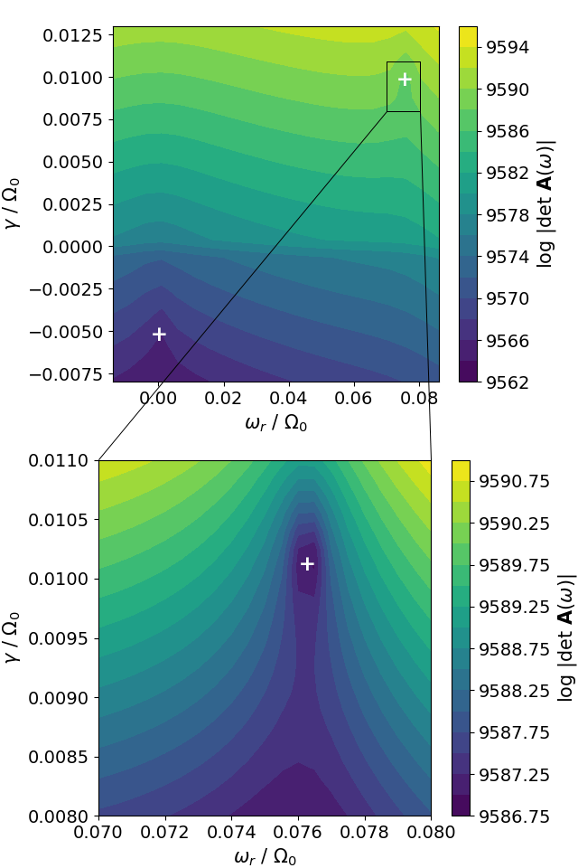
Figure 15: Local minima of $\log|\det\bm{A}(\omega_{r}+i\gamma)|$ for $A=0.8$, $\Delta w/H=1.5$, $St=0.03$, $\alpha=3\times 10^{-4}$, $f_{g\rm min}=0.7$, and $k=0.1$. The first panel shows two local minima (white plus signs) at $(0.000-0.005i)\Omega_{0}$ and $(0.076+0.010i)\Omega_{0}$. The second panel is an enlargement of the second local minimum, which corresponds to a Type II DRWI. We do not follow up the first minimum which is a decaying mode.

The method above allows us to visualise the distribution of possible eigenvalues $\omega$ and then to identify which one is desired, but is inefficient and non-automated. In particular, Muller’s method will not easily converge to the desired solution if the initial guesses are not in the small local minimum region, so one cannot start from an arbitrary guess. Therefore, after grasping the general distribution patterns of the eigenvalues, we use the following alternative method to evaluate $\omega_{m}$, which is fast, automatic, and only requires a rough initial estimate of $\omega_{m}$. Note that we have arranged Equations (54)–(57) such that the angular frequency appears only once in each equation and only takes the form $-i\omega$. In our construction of the matrix $\bm{A}(\omega)$, then, all $\omega$ lie on the diagonal as $-i\omega$ with the exception of eight boundary rows that involve nonlinear relations of $\omega$. This implies that $\bm{A}(\omega)\approx\bm{A}(0)-i\omega\bm{I}$, where $\bm{I}$ is the $4N\times 4N$ identity matrix. Therefore, the desired eigenvalue $\omega_{m}$ might be very close to another complex number $\lambda_{m}$, the latter satisfying

$$\det(\bm{A}(0)-i\lambda_{m}\bm{I})=0\ .$$ (93)

In other words, $i\omega_{m}$ is approximately equal to one of the eigenvalues, $i\lambda_{m}$, of the matrix $\bm{A}(0)$ (not to be confused with the eigenvalue of the perturbation problem). We verify by calculating all matrix eigenvalues that the approximation is valid for small $|\omega_{m}|$, which includes almost all cases of interest in this paper. In particular, choosing $\lambda_{m}$ and two arbitrary points nearby are generally found to be sufficient to ensure fast convergence toward $\omega_{m}$ using Muller’s method. One would in fact expect an exact equation of $\omega_{m}=\lambda_{m}$ if the boundary conditions were linear in $\omega$.

To obtain $\lambda_{m}$, we set a rough initial guess $\omega_{\rm guess}$ and find among the matrix eigenvalues the one closest to $i\omega_{\rm guess}$ on the complex plane. This is done using the shifted inverse power method (in ARPACK software, available via scipy.sparse.linalg.eigs). The resulting $\lambda_{m}$ and two arbitrary points nearby are then provided as initial guesses to Muller’s method to give the accurate $\omega_{m}$. The method will converge as long as $i\omega_{\rm guess}$ is closer to $i\lambda_{m}$ than any other irrelevant matrix eigenvalues, granting much greater tolerance compated to directly using Muller’s method. For example, in Figure 15, $\omega_{\rm guess}=(0.03+0.05i)\Omega_{0},(0.05+0i)\Omega_{0}$ or $(0.2+1i)\Omega_{0}$ all yield $\omega_{m}=(0.076+0.010i)\Omega_{0}$. In contrast, if we attempted to use Muller’s method directly, a deviation of $0.002\Omega_{0}$ of the initial guesses from the true root would almost certainly fail the algorithm.

We first noticed the Type II DRWI by brute-force scan in the $\omega_{r}$–$\gamma$ plane before developing the method above, but the discovery would have been very straightforward by noting two distinct types of $\lambda_{m}$ with positive imaginary parts among all matrix eigenvalues. Also, as one progressively increases $k$, no new unstable candidates showed up from the matrix eigenvalues. This, along with a few confirmatory brute-force scans at high $k$ that show no evidence of new roots, indicates that short-range instabilities unlikely exist in our setting.

After obtaining $\omega_{m}$, we proceed to solve the eigenfunction $\vec{u}_{1m}(x,\omega_{m})$, following Ono et al. (2016), by introducing a random vector with a norm of order the machine precision on the right-hand side of Equation (92) and then solving the linear equation with LAPACK (via scipy.linalg.solve). An alternative method is to calculate the eigenvector of $\bm{A}(\omega_{m})$ of matrix eigenvalue zero, which yields the same result.

Appendix D Bifurcation of the two types of instabilities

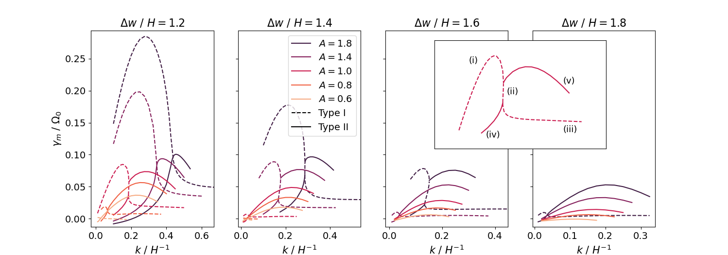
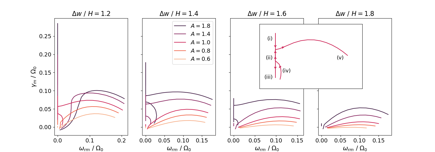
Figure 16: Dispersion relation of different pressure bumps with $f_{g\rm min}=0.7,St=0.03$, and $\alpha=1\times 10^{-4}$. Inset boxes on the upper and lower right specifically display $A=1.0$ and $\Delta w/H=1.2$ as an example. The Type I modes for $A=1.6,\Delta w/H\leq 1.0$ and for $A=1.8,\Delta w/H\leq 1.4$ are stable and hence not shown. Top: growth rate $\gamma_{m}$ versus azimuthal wavenumber $k$. Bottom: $\gamma_{m}$ versus phase angular velocity $\omega_{rm}$ of the instability. Type II modes with negative $\omega_{rm}$ are not drawn. Arrows in the inset box mark the direction of increasing $k$. See text for the explanation of segments (i) to (v).

Despite the neat distinction in Figure 2, the Type I and II DRWIs are subtly intertwined in a broader parameter space, especially for moderately large $A$ and small $\Delta w$ combined with large $St$ and small $\alpha$. Shown in Figure 16 is a collection of dispersion relations of various pressure bump heights and widths. The dispersion relation may be thought of residing in the 3D space of $(k,\omega_{rm},\gamma_{m})$, of which we display the 2D projections. Within the parameter space explored in this work, we categorise these conditions as follows:

a) Moderately smooth bumps, e.g., $A=0.6,\Delta w/H=1.2$, or $A=1.8,\Delta w/H=1.8$. The setting in Figure 2 also belongs to this group. The Type I DRWI has slow growth rates while the Type II shows one single curve in the $(k,\omega_{rm},\gamma_{m})$ space with a maximum $\gamma_{m}$. The curves of these two modes do not intersect in the 3D space. In other words, it is impossible to switch from one type to the other continuously: as $k$ increases, the real part of the Type I eigenvalue remains zero but that of the Type II monotonically deviates from zero. However, a kink emerges from, e.g., the Type II $\gamma_{m}$–$\omega_{rm}$ curve of $A=0.8,\Delta w/H=1.2$ at $(\omega_{rm}/\Omega_{0},\gamma_{m}/\Omega_{0})=(0.01,0.01)$, which heralds the reversal of the Type II curve towards $\omega_{rm}=0$ for sharper bumps.

b) Moderately sharp bumps, e.g., $A=1.0,\Delta w/H=1.2$, or $A=1.8,\Delta w/H=1.6$. In the $\gamma_{m}$–$\omega_{rm}$ plot, the kink described above develops until touching the $y$-axis, forming two bifurcation points with the Type I curve. The trend is best understood viewing the bottom inset panel in Figure 16. Initially ($k\ll 1$), the Type II mode corresponds to the lower end of the branch (iv). With the continuous increase of $k$ (along the arrow), the phase angular velocity reaches a local maximum before reducing to zero. Now, upon arrival at the lower bifurcation point, an additional increment of $k$ may lead the curve to two directions: upwards, i.e., branch (ii), or downwards, i.e., branch (iii). Importantly, both have $\omega_{rm}=0$ and hence are Type I, indicating a type transition. Along the branch (ii), further increase of $k$ encounters the descending Type I branch (i) at the upper bifurcation point. Another type transition occurs here with the emergence of the Type II branch (v). In short, the previously monolithic Type II curve is now inserted with a Type I segment (ii).

The description above traces the increase of $k$ along branches (iv)–(ii)–(v). Alternatively, from the perspective of the $\gamma_{m}$–$k$ plot, one may imagine that the branches (i)–(ii)–(iii) and the branches (iv)–(v) previously rested in different planes in the 3D space and thus did not interfere with each other. Enhancement of the bump sharpness, however, brings the two curves to the same plane, and the Type I curve cuts the Type II curve into two pieces (iv) and (v) while itself distorted. Indeed, at the bifurcation points, the Type I branches (i) and (ii) or (ii) and (iii) are connected without abrupt turning, but branch (iv) or (v) shoots off obliquely (not tangential to other branches). The Type I trend in the $\gamma_{m}$–$k$ plot can therefore be described as an upward convex (i) followed by a temporary reversal (ii) and then a flat tail (iii).

We only show the Type II modes with positive $\omega_{rm}$ in Figure 16. The negative counterpart would overlap with the shown Type II curves in the $\gamma_{m}$–$k$ plots and would appear as mirrored images of the positive-$\omega_{rm}$ Type II curves about the $y$-axis in the $\gamma$–$\omega_{rm}$ plots. This reconciles with the mathematical notion that a bifurcation point should have two inbound and two outbound branches.

c) Very sharp bumps, e.g., $A=1.4,\Delta w/H=1.2$. The two types of modes again have independent curves. In the $\gamma_{m}$–$k$ plot, the Type I curve still has a maximum followed by a long tail, whereas the low-$k$ flank of the Type II curve becomes concave up (showing a positive second derivative).

The smooth shift between the two types of instabilities implies a smooth transition of the instability mechanism. In a transition from Type II to Type I, the eigenmodal phase velocity $\omega_{rm}/k$ gradually reduces to zero, and the co-rotation radius moves from outside to the center of the dust bump. Also, cross-correlation calculations similar to those in Section 5.4.2 show that the phase difference between $q_{1}$ and $S_{\rm bar1}$ rapidly increases from a small angle to well over $90^{\circ}$; meanwhile, the phase difference between the vortensity perturbation and advection diminishes to zero. This indicates that, during the transition, advection takes over the role from the baroclinic source in driving the instability in the dust bump, as might be expected. Further studies of the mechanism behind the bifurcation would be more complex and lie beyond the scope of this paper.

Appendix E Tentative propagation mechanism of the Type II DRWI

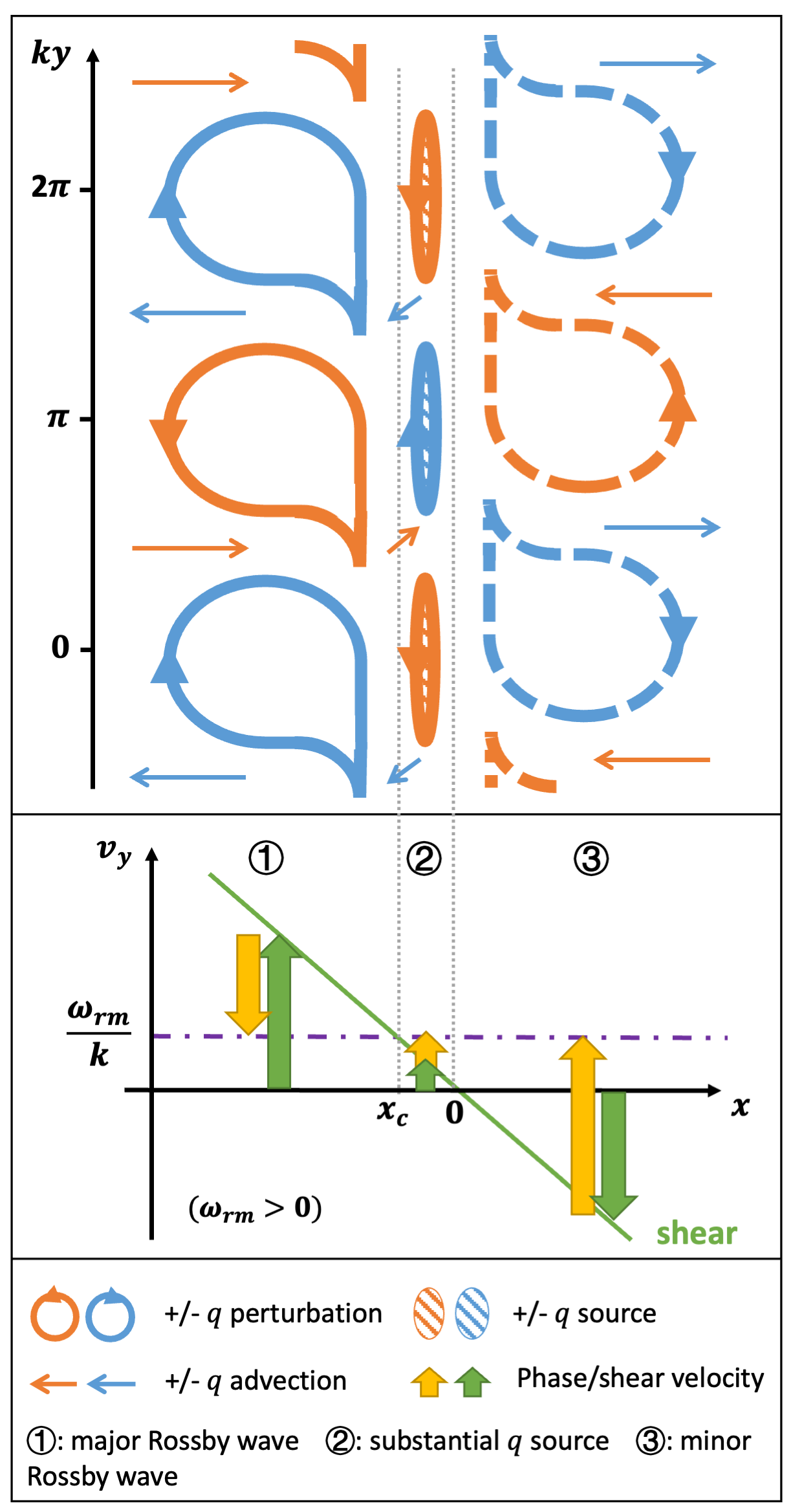
Figure 17: Schematic illustration of the tentative propagation mechanism of the Type II DRWI in the rotating frame with $\omega_{rm}>0$. Top: vortensity perturbation, advection and source patterns on the $x$-$y$ plane, extracted from Figure 5. The patterns are separated by grey dotted lines into three regions, namely, {1}⃝, {2}⃝, and {3}⃝ from left to right. Bottom: velocity decomposition in each region. The phase and shear velocities combine to give the modal azimuthal velocity $\omega_{rm}/k$. The two panels share the $x$-axis.

One main feature of the Type II DRWI is a non-zero phase velocity. We have explained the propagation of perturbation patterns in the dust bump in Section 5.4, but the Rossby waves are also important components of this instability. Here, we tentatively explain the propagation of the Type II DRWI with the entire mode in mind, as illustrated in Figure 17. With a simplified physical picture, we focus on how the different components share one modal phase velocity despite (or perhaps as a result of) the asymmetric eigenfunction patterns.

We first apply the interpretation in Ono et al. (2016) to explain the propagation of the gas perturbation patterns. In the following, we will use the words “upper” and “lower” to describe location with higher or lower $y$-coordinate. The leftmost region (labelled as {1}⃝) in the top panel in Figure 17, where $f_{d}\ll 1$ and the background vortensity satisfies $dq_{0}/dx<0$, illustrates a Rossby wave with a negative phase velocity $v_{\rm phase}$ in $\hat{y}$. For sake of explanation, we temporarily ignore any interaction between regions {1}⃝ and {2}⃝. Positive vortensity perturbations imply clockwise loops of gas flow, while negative counterclockwise. Such flows drive $\hat{x}$-direction advection of vortensity along the $q_{0}$ gradient, which induces $y$-direction migration of the loops themselves. For example, the flows at $ky\sim\pi/2$ and $ky\sim 3\pi/2$ in region ① increase and decrease local vortensity respectively, the former extending the lower side of the $+q_{1}$ loop and the latter paring the upper side. The result is a downward shift of the perturbation patterns. However, here the Rossby wave travels on a background with shear velocity $v_{\rm shear}=v^{\prime}_{0y}-3\Omega_{0}x/2$, and thus the patterns overall move upwards in the frame co-rotating with $x=0$.

The decomposition of the motion of the Rossby wave into $v_{\rm phase}$ and $v_{\rm shear}$ is essentially built in the vortensity equation (34). Formally, the phase velocity of the Rossby wave can be defined as

$$v_{\rm phase}={\rm Re}\left[i\frac{-(dq_{0}/dx)v^{\prime}_{1x}}{kq_{1}}\right]\ ,$$ (94)

where the numerator appeared in Equation (34) as the radial advection term. Replacing it with the full vortensity advection term would recover $\omega_{rm}/k$ assuming conservation of vortensity, while replacing it with the azimuthal advection term would give $v_{\rm shear}$. Equation (94) implies that, when vortensity is conserved, $v_{\rm phase}$ will depend on the strength of the radial vortensity advection relative to that of the vortensity perturbation.

Application of the argument above on both regions {1}⃝ and {3}⃝ gives two Rossby waves with $v_{\rm phase}$ in the opposite direction. In region {1}⃝ resides what we term the “major Rossby wave” (solid) with much more conspicuous perturbation compared to the “minor Rossby wave” (dashed) in region {3}⃝. However, the $x$-direction vortensity advection has comparable strengths in the two regions, hence more influential relative to the minor Rossby wave in terms of shifting the perturbation patterns. This leads to a faster phase velocity in region ③, as illustrated in the bottom panel in Figure 17. Then, taking the similar but opposite shearing velocity into account, one observes that $|v_{\rm phase,{3}⃝}|>|v_{\rm shear,{3}⃝}|\simeq|v_{\rm shear,{1}⃝}|>|v_{\rm phase,{1}⃝}|$.This explains why the two regions share an overall modal phase velocity $\omega_{rm}/k=v_{\rm phase,{3}⃝}-v_{\rm shear,{3}⃝}=v_{\rm shear,{1}⃝}-v_{\rm phase,{1}⃝}$. Our explanation suggests a close link between the non-zero real part of the eigenvalue and the asymmetry of the eigenfunction.

The propagation of $q_{1}$ patterns in region ② also fits in this picture. As shown in Section 5.4, here the vortensity advection governs the propagation with a $\sim 90^{\circ}$ spatial phase lead over $q_{1}$, thus inducing the $\pm q_{1}$ loops in region ② to travel upwards. This process is similar to that of the Rossby wave, except that the background $v_{\rm shear}$ is now in the same direction as $v_{\rm phase}$. Here, the material flow advects vortensity across different regions (e.g., the inclined arrows between region ① and ② in Figure 17), indicating a close interaction between the Rossby wave and the dust bump.

References

- ALMA Partnership et al. (2015) ALMA Partnership et al., 2015, ApJ, 808, L3
- Andrews (2020) Andrews S. M., 2020, ARA&A, 58, 483
- Andrews et al. (2018) Andrews S. M., et al., 2018, ApJ, 869, L41
- Auffinger & Laibe (2018) Auffinger J., Laibe G., 2018, MNRAS, 473, 796
- Bae et al. (2016) Bae J., Zhu Z., Hartmann L., 2016, ApJ, 819, 134
- Bae et al. (2022) Bae J., Isella A., Zhu Z., Martin R., Okuzumi S., Suriano S., 2022, arXiv e-prints, p. arXiv:2210.13314
- Baer (2018) Baer M., 2018, findiff Software Package, https://github.com/maroba/findiff
- Bai & Stone (2010) Bai X.-N., Stone J. M., 2010, ApJ, 722, 1437
- Batygin & Morbidelli (2023) Batygin K., Morbidelli A., 2023, Nature Astronomy, 7, 330
- Birnstiel et al. (2012) Birnstiel T., Klahr H., Ercolano B., 2012, A&A, 539, A148
- Boehler et al. (2017) Boehler Y., Weaver E., Isella A., Ricci L., Grady C., Carpenter J., Perez L., 2017, ApJ, 840, 60
- Carrera et al. (2015) Carrera D., Johansen A., Davies M. B., 2015, A&A, 579, A43
- Carrera et al. (2021) Carrera D., Simon J. B., Li R., Kretke K. A., Klahr H., 2021, AJ, 161, 96
- Chang & Oishi (2010) Chang P., Oishi J. S., 2010, ApJ, 721, 1593
- Chang et al. (2023) Chang E., Youdin A. N., Krapp L., 2023, ApJ, 946, L1
- Chen & Lin (2020) Chen K., Lin M.-K., 2020, ApJ, 891, 132
- Cimerman & Rafikov (2023) Cimerman N. P., Rafikov R. R., 2023, MNRAS, 519, 208
- Crnkovic-Rubsamen et al. (2015) Crnkovic-Rubsamen I., Zhu Z., Stone J. M., 2015, MNRAS, 450, 4285
- Dubrulle et al. (1995) Dubrulle B., Morfill G., Sterzik M., 1995, Icarus, 114, 237
- Dullemond et al. (2018) Dullemond C. P., et al., 2018, ApJ, 869, L46
- Facchini et al. (2020) Facchini S., et al., 2020, A&A, 639, A121
- Flaherty et al. (2020) Flaherty K., et al., 2020, ApJ, 895, 109
- Fu et al. (2014a) Fu W., Li H., Lubow S., Li S., 2014a, ApJ, 788, L41
- Fu et al. (2014b) Fu W., Li H., Lubow S., Li S., Liang E., 2014b, ApJ, 795, L39
- Gholipour & Nejad-Asghar (2014) Gholipour M., Nejad-Asghar M., 2014, MNRAS, 441, 1910
- Hammer & Lin (2023) Hammer M., Lin M.-K., 2023, arXiv e-prints, p. arXiv:2304.01674
- Hammer et al. (2021) Hammer M., Lin M.-K., Kratter K. M., Pinilla P., 2021, MNRAS, 504, 3963
- Harris et al. (2020) Harris C. R., et al., 2020, Nature, 585, 357
- Hashimoto et al. (2021) Hashimoto J., Muto T., Dong R., Liu H. B., van der Marel N., Francis L., Hasegawa Y., Tsukagoshi T., 2021, ApJ, 911, 5
- Hsu & Lin (2022) Hsu C.-Y., Lin M.-K., 2022, ApJ, 937, 55
- Huang & Bai (2022) Huang P., Bai X.-N., 2022, ApJS, 262, 11
- Huang et al. (2020) Huang P., Li H., Isella A., Miranda R., Li S., Ji J., 2020, ApJ, 893, 89
- Hunter (2007) Hunter J. D., 2007, Computing in Science & Engineering, 9, 90
- Jacquet et al. (2011) Jacquet E., Balbus S., Latter H., 2011, MNRAS, 415, 3591
- Jiang & Ormel (2023) Jiang H., Ormel C. W., 2023, MNRAS, 518, 3877
- Johansen et al. (2009) Johansen A., Youdin A., Mac Low M.-M., 2009, ApJ, 704, L75
- Klahr & Schreiber (2020) Klahr H., Schreiber A., 2020, ApJ, 901, 54
- Laibe & Price (2014) Laibe G., Price D. J., 2014, MNRAS, 444, 1940
- Laune et al. (2020) Laune J., Li H., Li S., Li Y.-P., Walls L. G., Birnstiel T., Drążkowska J., Stammler S., 2020, ApJ, 889, L8
- Lehmann & Lin (2022) Lehmann M., Lin M. K., 2022, A&A, 658, A156
- Lesur et al. (2022) Lesur G., et al., 2022, arXiv e-prints, p. arXiv:2203.09821
- Li & Youdin (2021) Li R., Youdin A. N., 2021, ApJ, 919, 107
- Li et al. (2000) Li H., Finn J. M., Lovelace R. V. E., Colgate S. A., 2000, ApJ, 533, 1023
- Li et al. (2019) Li Y.-P., et al., 2019, ApJ, 878, 39
- Li et al. (2020) Li Y.-P., Li H., Li S., Birnstiel T., Drążkowska J., Stammler S., 2020, ApJ, 892, L19
- Lin (2014) Lin M.-K., 2014, MNRAS, 437, 575
- Lin (2019) Lin M.-K., 2019, MNRAS, 485, 5221
- Lin & Youdin (2017) Lin M.-K., Youdin A. N., 2017, ApJ, 849, 129
- Long et al. (2022) Long F., et al., 2022, ApJ, 937, L1
- Lovascio et al. (2022) Lovascio F., Paardekooper S.-J., McNally C., 2022, MNRAS, 516, 1635
- Lovelace et al. (1999) Lovelace R. V. E., Li H., Colgate S. A., Nelson A. F., 1999, ApJ, 513, 805
- Lyra et al. (2009) Lyra W., Johansen A., Klahr H., Piskunov N., 2009, A&A, 493, 1125
- Lyra et al. (2018) Lyra W., Raettig N., Klahr H., 2018, Research Notes of the American Astronomical Society, 2, 195
- Masset (2000) Masset F., 2000, A&AS, 141, 165
- Meheut et al. (2012) Meheut H., Meliani Z., Varniere P., Benz W., 2012, A&A, 545, A134
- Miranda et al. (2017) Miranda R., Li H., Li S., Jin S., 2017, ApJ, 835, 118
- Ono et al. (2016) Ono T., Muto T., Takeuchi T., Nomura H., 2016, ApJ, 823, 84
- Pan & Yu (2020) Pan L., Yu C., 2020, ApJ, 898, 7
- Pinilla & Youdin (2017) Pinilla P., Youdin A., 2017, in Pessah M., Gressel O., eds, Astrophysics and Space Science Library Vol. 445, Formation, Evolution, and Dynamics of Young Solar Systems. p. 91, doi:10.1007/978-3-319-60609-5_4
- Pinilla et al. (2012) Pinilla P., Birnstiel T., Ricci L., Dullemond C. P., Uribe A. L., Testi L., Natta A., 2012, A&A, 538, A114
- Rometsch et al. (2021) Rometsch T., Ziampras A., Kley W., Béthune W., 2021, A&A, 656, A130
- Rosotti et al. (2020) Rosotti G. P., Teague R., Dullemond C., Booth R. A., Clarke C. J., 2020, MNRAS, 495, 173
- Schreiber & Klahr (2018) Schreiber A., Klahr H., 2018, ApJ, 861, 47
- Squire & Hopkins (2018) Squire J., Hopkins P. F., 2018, MNRAS, 477, 5011
- Stone & Gardiner (2010) Stone J. M., Gardiner T. A., 2010, ApJS, 189, 142
- Stone et al. (2008) Stone J. M., Gardiner T. A., Teuben P., Hawley J. F., Simon J. B., 2008, ApJS, 178, 137
- Stone et al. (2020) Stone J. M., Tomida K., White C. J., Felker K. G., 2020, The Astrophysical Journal Supplement Series, 249, 4
- Surville et al. (2020) Surville C., Mayer L., Alibert Y., 2020, arXiv e-prints, p. arXiv:2009.04775
- Tominaga et al. (2019) Tominaga R. T., Takahashi S. Z., Inutsuka S.-i., 2019, ApJ, 881, 53
- Umurhan et al. (2020) Umurhan O. M., Estrada P. R., Cuzzi J. N., 2020, ApJ, 895, 4
- Virtanen et al. (2020) Virtanen P., et al., 2020, Nature Methods, 17, 261
- Woo et al. (2023) Woo J. M. Y., Morbidelli A., Grimm S. L., Stadel J., Brasser R., 2023, Icarus, 396, 115497
- Xu & Bai (2022a) Xu Z., Bai X.-N., 2022a, ApJ, 924, 3
- Xu & Bai (2022b) Xu Z., Bai X.-N., 2022b, ApJ, 937, L4
- Yang & Zhu (2020) Yang C.-C., Zhu Z., 2020, MNRAS, 491, 4702
- Yang et al. (2017) Yang C.-C., Johansen A., Carrera D., 2017, A&A, 606, A80
- Youdin & Goodman (2005) Youdin A. N., Goodman J., 2005, ApJ, 620, 459
- Zhu et al. (2014) Zhu Z., Stone J. M., Rafikov R. R., Bai X.-n., 2014, ApJ, 785, 122
- de Val-Borro et al. (2007) de Val-Borro M., Artymowicz P., D’Angelo G., Peplinski A., 2007, A&A, 471, 1043
- van der Marel et al. (2021) van der Marel N., et al., 2021, AJ, 161, 33