Electron-ion heating partition in imbalanced solar-wind turbulence

Abstract

A likely candidate mechanism to heat the solar corona and solar wind is low-frequency “Alfvénic” turbulence sourced by magnetic fluctuations near the solar surface. Depending on its properties, such turbulence can heat different species via different mechanisms, and the comparison of theoretical predictions to observed temperatures, wind speeds, anisotropies, and their variation with heliocentric radius provides a sensitive test of this physics. Here we explore the importance of normalized cross helicity, or imbalance, for controlling solar-wind heating, since it is a key parameter of magnetized turbulence and varies systematically with wind speed and radius. Based on a hybrid-kinetic simulation in which the forcing’s imbalance decreases with time—a crude model for a plasma parcel entrained in the outflowing wind—we demonstrate how significant changes to the turbulence and heating result from the “helicity barrier” effect. Its dissolution at low imbalance causes its characteristic features—strong perpendicular ion heating with a steep “transition-range” drop in electromagnetic fluctuation spectra—to disappear, driving more energy into electrons and parallel ion heat, and halting the emission of ion-scale waves. These predictions seem to agree with a diverse array of solar-wind observations, offering to explain a variety of complex correlations and features within a single theoretical framework.

1 Introduction

The solar corona and its extended outflow, the solar wind, provide us with an unparalleled laboratory for studying the physics of magnetized collisionless plasmas. Decades of observations have revealed a highly complex system filled with electromagnetic fluctuations across a vast range of scales, whose properties (e.g., total power or spectra) are correlated in surprising and nontrivial ways with the plasma’s flow speed, temperatures, anisotropies, and elemental abundances (Marsch, 2006; Horbury et al., 2012; Bruno & Carbone, 2013). These correlations, as well as the extended heating at large heliocentric distances needed to explain the high speed of fast-wind streams (Parker, 1965), suggest that the solar wind is shaped by both properties of its low-coronal source and turbulent heating at larger altitudes. Of particular interest are the decades of observations that hint at the role played by the fluctuations’ imbalance (i.e., normalized cross helicity), a key parameter in the theory of magnetized turbulence (Dobrowolny et al., 1980; Schekochihin, 2022) that is observed to correlate with wind speed $U$ and decrease with increasing heliocentric radius $R$ (e.g., Roberts et al., 1987; Marsch, 2006; D’Amicis et al., 2021).

In this Letter, we argue for the importance of imbalance in shaping turbulence and heating in the low-$\beta$ solar wind. We focus on the physics of the “helicity barrier” (Meyrand et al., 2021), which dramatically alters imbalanced turbulence in $\beta\lesssim 1$ plasmas by restricting the turbulent energy cascade at perpendicular scales $\lambda_{\perp}$ below the ion gyroradius $\rho_{i}$. Previous kinetic simulations have shown how numerous features of helicity-barrier-mediated turbulence match measurements of the low-$\beta$ solar wind well (Squire et al., 2022; hereafter S+22), including properties of the steep “transition-range” drop in electromagnetic field spectra around $\rho_{i}$ scales and the ion velocity distribution function (VDF; see, e.g., Duan et al., 2021; Bowen et al., 2022, 2023).

We study how the turbulence evolves as imbalance is slowly decreased in time, transitioning between the highly imbalanced and balanced regimes. This physics is of interest for two reasons: first, it is a crude model for the expected response of the turbulent heating as the plasma flies outwards from the Sun and its imbalance decreases; second, it captures how the helicity barrier becomes weaker and eventually disappears at low imbalance, thus probing its robustness. The results, which are based on a kinetic simulation of forced Alfvénic turbulence, can explain the observed correlation of wind speed with ion temperatures, as well as the switch from negative to positive correlation of wind speed with electron temperature at increasing $R$ (e.g., Burlaga & Ogilvie, 1973; Marsch et al., 1989; Shi et al., 2023; Bandyopadhyay et al., 2023). Correlations with other properties such as the spectral transition range, proton VDFs, and plasma-wave/instability activity seem to explain a diverse array of observations within a single theoretical framework.

2 Formulation of the problem and method of solution

2.1 The helicity barrier

The helicity barrier arises due to the conservation of a “generalized helicity” $\mathcal{H}$ in low-$\beta$ gyrokinetics (Schekochihin et al., 2019; Meyrand et al., 2021). At large scales $\lambda_{\perp}\gg\rho_{i}$, $\mathcal{H}$ is the cross helicity, which, along with the energy, cascades forward to smaller scales; at small scales $\lambda_{\perp}\ll\rho_{i}$, $\mathcal{H}$ is a form of magnetic helicity, which cannot cascade to smaller $\lambda_{\perp}$ without violating energy conservation (Fjørtoft, 1953). Thus, the sub-$\rho_{i}$ cascade must have $\mathcal{H}=0$, restricting its energy flux to be at most the “balanced portion” of that injected, $\varepsilon-\varepsilon_{H}$, where $\varepsilon$ and $\varepsilon_{H}$ are the large-scale injection rates of energy and helicity, respectively. The remaining energy input, $\varepsilon-(\varepsilon-\varepsilon_{H})=\varepsilon_{H}$, is “trapped” at $\lambda_{\perp}\lesssim\rho_{i}$ scales, causing the turbulence to reach large amplitudes and (through critical balance) small parallel scales approaching the ion inertial length $d_{i}$. The fluctuations then take on the character of oblique ion-cyclotron waves (ICWs) with frequencies $\omega$ that approach the ion gyrofrequency $\Omega_{i}$. This activates strong wave-particle interactions and quasi-linear resonant heating (Kennel & Engelmann, 1966), which can absorb the remaining energy input, allowing the turbulence to saturate (Li et al., 1999). It also causes the plasma to become unstable and emit small-scale parallel ICWs (Chandran et al., 2010b). By diverting a large fraction of the energy flux that would have reached electron scales, and thus electron heat, into ions instead, the helicity barrier causes large ion-to-electron heating ratios $Q_{i}/Q_{e}\simeq\varepsilon_{H}/(\varepsilon-\varepsilon_{H})$ in anisotropic low-$\beta$ turbulence.

2.2 Numerical method

We use the hybrid-kinetic method implemented in the Pegasus++ code (Kunz et al., 2014; Arzamasskiy et al., 2023). This approach treats the ion (proton) dynamics fully kinetically using a particle-in-cell (PIC) approach, while the electrons constitute a massless, neutralizing, isothermal fluid. The ion macro-particle positions ($\bm{r}$) and velocities ($\bm{v}$) are drawn from an initially Maxwellian $f_{i}(\mbox{\boldmath{$v$}})$ and evolved via

$$\frac{{\rm d}\bm{r}}{{\rm d}t}=\bm{v},\quad\frac{{\rm d}\bm{v}}{{\rm d}t}=\frac{e}{m_{i}}\left[\bm{E}(\bm{r},t)+\frac{\bm{v}}{c}\,\mbox{\boldmath{$\times$}}\,\bm{B}(\bm{r},t)\right]+\frac{1}{m_{i}}\bm{F}_{\perp}^{U},$$ (1)

where $E$ and $B$ are the electric and magnetic fields and $\bm{F}_{\perp}^{U}$ stirs turbulence by injecting incompressible motions perpendicular (“$\perp$”) to a mean (“guide”) magnetic field $\bm{B}_{0}$. The magnetic field satisfies a modified version of Faraday’s law,

$$\frac{\partial\bm{B}}{\partial t}=-c\mbox{\boldmath{$\nabla$}}\,\mbox{\boldmath{$\times$}}\,(\bm{E}+\bm{F}_{\perp}^{B})+\eta_{4}\nabla^{4}\bm{B},$$ (2)

where $\bm{F}_{\perp}^{B}$ forces solenoidal magnetic fluctuations perpendicular to $\bm{B}_{0}$ and $\eta_{4}$ is a hyper-resistivity that absorbs small-scale magnetic energy. The electric field is

$$\bm{E}=-\frac{\bm{u}}{c}\,\mbox{\boldmath{$\times$}}\,\bm{B}-\frac{T_{e}}{en}\mbox{\boldmath{$\nabla$}}{n}+\frac{(\mbox{\boldmath{$\nabla$}}\,\mbox{\boldmath{$\times$}}\,\bm{B})\,\mbox{\boldmath{$\times$}}\,\bm{B}}{4\pi en},$$ (3)

where $n$ is the ion (and electron) density and $\bm{u}$ is the ion flow velocity, both of which are computed via a weighted sum of the macro-particles in the relevant region of space; $T_{e}$ is the electron temperature, which is a parameter of the model; and $e$, $m_{i}$, and $c$ are the electron/ion charge, the ion mass, and the speed of light, respectively. We also define the Alfvén speed $v_{\rm A}\equiv B_{0}/\sqrt{4\pi nm_{i}}$, $\Omega_{i}\equiv eB_{0}/(m_{i}c)$, the ion thermal speed $v_{\rm th}$, and the “Elsässer” fields $\bm{z}^{\pm}\equiv\bm{u}_{\perp}\pm\bm{B}_{\perp}/\sqrt{4\pi nm_{i}}\equiv\bm{u}_{\perp}\pm\bm{b}_{\perp}$. Volume averages are denoted by $\langle\,\cdot\,\rangle$ and $f_{i}(w_{\perp},w_{\|})$ is the gyro-averaged VDF, with $w_{\perp}$ and $w_{\|}$ the particle velocities perpendicular and parallel to the local magnetic field in the frame of the plasma (i.e., $\bm{w}\equiv\bm{v}-\bm{u}$).

2.3 Problem set up

Our basic simulation set up follows S+22. The simulation represents a small co-moving patch of plasma, capturing realistic solar-wind turbulence amplitudes and anisotropies around $k_{\perp}\rho_{i}\sim 1$ scales, where $k_{\perp}\sim 1/\lambda_{\perp}$ denotes the perpendicular wavenumber. The domain is Cartesian and periodic, with coordinates $\{x,y,z\}$, and is elongated along $\bm{B}_{0}=-B_{0}\hat{\mbox{\boldmath{$z$}}}$, with $L_{z}=6L_{\perp}$ and $L_{\perp}=67.5d_{i}$ ($d_{i}=v_{\rm A}/\Omega_{i}$). With these parameters, the box shape approximately matches the (statistical) shape of turbulent eddies measured at similar scales in the solar wind (Chen et al., 2016; S+22). The grid resolution is $N_{\perp}^{2}\times N_{z}=392^{2}\times 2352$, so that the smallest resolved scales are $k_{\perp,{\rm max}}d_{i}\simeq\pi N_{\perp}d_{i}/L_{\perp}\approx 18$. We use $N_{\rm ppc}=216$ ion-macro-particles per cell. The hyper-resistivity was increased from $\eta_{4}\approx 2.4\times 10^{-5}d_{i}^{4}\Omega_{i}$ to $\eta_{4}=5\times 10^{-5}d_{i}^{4}\Omega_{i}$ at $t=4.3\tau_{\rm A}$ in response to the strengthening kinetic-range cascade.

The simulation is initialized at $t=0$ using the final snapshot from S+22, and thus represents saturated highly imbalanced turbulence with strong perpendicular ion heating and a helicity barrier, similar to turbulence observed in the near-Sun solar wind by PSP (Bowen et al., 2023). The initial ion temperature is such that $\beta_{i}=8\pi\langle nT_{i}\rangle/\langle B^{2}\rangle\approx 0.33$; electrons are isothermal with $\beta_{e0}=8\pi\langle n\rangle T_{e}/B_{0}^{2}=0.3$. The simulation is run for an additional ${\approx}18\tau_{\rm A}$, where $\tau_{\rm A}=L_{z}/v_{\rm A}$ is the outer-scale Alfvén time, which is also comparable to the turnover time of the turbulence $\tau_{\rm turb}\sim L_{\perp}/u_{{\rm rms}}$ due to our choice of forcing parameters (see below; $u_{{\rm rms}}=\langle u^{2}\rangle^{1/2}$ is the root-mean-square velocity). Because the ions heat up, $\beta_{i}$ increases over the course of the simulation to ${\simeq}0.45$ and $\rho_{i}=\sqrt{\beta_{i}}d_{i}$ changes modestly. The domain resolves scales between $k_{\perp 0}\rho_{i0}\equiv 2\pi\rho_{i0}/L_{\perp}\approx 0.05$ and $k_{\perp{\rm max}}\rho_{i0}\approx 10$, where $\rho_{i0}=\rho_{i}(t=0)$.

2.4 Decreasing imbalance with distance from the Sun

A novel feature of this work is the forcing, which changes from imbalanced to balanced over the simulation, heuristically mimicking the radial evolution of the solar wind. We inject energy and cross helicity at the rates $\varepsilon$ and $\varepsilon_{H}$, respectively, with forcing functions $\bm{F}_{\perp}^{U}$ and $\bm{F}_{\perp}^{B}$ that are intended to capture the effect of stirring due to turbulent eddies above the box scale. These consist of random combinations of large-scale Fourier modes with wavenumbers $k_{j}$ satisfying $2\pi/L_{j}\leq k_{j}\leq 4\pi/L_{j}$ for $j=\{x,y,z\}$. They are computed as $\bm{F}_{\perp}^{U}=f^{U}\bm{F}_{0}$ and $\mbox{\boldmath{$\nabla$}}\,\mbox{\boldmath{$\times$}}\,\bm{F}_{\perp}^{B}=f^{B}\bm{F}_{0}$, where $\bm{F}_{0}$ is divergence-free, perpendicular to $\bm{B}_{0}$, and evolved in time via an Ornstein–Uhlenbeck process with correlation time $\tau_{\rm A}/2$. We fix $\varepsilon$ and $\varepsilon_{H}$ at each time step by adjusting $f^{U}$ and $f^{B}$ so that $n\bm{u}\,\mbox{\boldmath{$\cdot$}}\,\bm{F}_{\perp}^{U}$ and $\bm{B}\,\mbox{\boldmath{$\cdot$}}\,\mbox{\boldmath{$\nabla$}}\,\mbox{\boldmath{$\times$}}\,\bm{F}_{\perp}^{B}$ take the values needed to inject the required energies into $\bm{z}^{\pm}$. $\bm{F}_{\perp}^{B}$ is computed from $\bm{F}_{0}$ via a fast Fourier transform and used in the standard Pegasus++ constrained-transport algorithm to evolve $\bm{B}$, ensuring that $\mbox{\boldmath{$\nabla$}}\,\mbox{\boldmath{$\cdot$}}\,\bm{B}=0$ to machine precision.

We fix $\varepsilon=C_{\rm A}m_{i}n(L_{\perp}/L_{z})^{2}v_{\rm A}^{2}V/\tau_{\rm A}\approx 37m_{i}nv_{\rm A}^{2}\Omega_{i}d_{i}^{3}$, where $C_{\rm A}=0.29$ is the Kolmogorov constant and $V$ is the simulation volume; the factor $(L_{\perp}/L_{z})^{2}v_{\rm A}^{2}/\tau_{\rm A}$ guarantees critically balanced fluctuations at the outer scale with $u_{\rm rms}\sim(L_{\perp}/L_{z})v_{\rm A}$ and $\tau_{\rm turb}\sim\tau_{\rm A}$. In contrast, $\varepsilon_{H}$ decreases in time during the simulation so that the “injection imbalance” $\varepsilon_{H}/\varepsilon$ starts at $0.9$ (as in S+22) then decreases linearly in time at a rate of $0.1$ every $1.5\tau_{\rm A}$, reaching $\varepsilon_{H}=0$ (balanced forcing) at $t=13.5\tau_{\rm A}$, where it remains for the rest of the simulation (see Fig. 1). Because the cross helicity and energy are approximately conserved at $k_{\perp}\rho_{i}\ll 1$ scales, this evolution is intended to mimic crudely the effect of larger scales becoming more balanced with radius, thereby driving the smaller scales with decreasing $\varepsilon_{H}/\varepsilon$. However, in the actual solar wind, the timescale over which the imbalance decreases is comparable to both the turbulent decay timescale and the expansion timescale $\tau_{\rm exp}\approx R/U$ (Roberts et al., 1987; Meyrand et al., 2023). By keeping $\varepsilon$ fixed, we effectively assume that the turbulent decay and expansion are slow compared to the simulation’s duration, which is appropriate since $\tau_{\rm exp}/\tau_{\rm A}\simeq 1300\,(B/80~{}{\rm nT})(R/35~{}{\rm R}_{\odot})(U/350~{}{\rm km~{}s}^{-1})^{-1}$ (see e.g., Bale et al. 2019). However, this also implies that our adopted imbalance-decrease timescale of ${\approx}15\tau_{\rm A}$ is too short. This trade-off is unavoidable given the extreme computational expense of kinetic-turbulence simulations, but it should be kept mind that the simulation can only qualitatively capture realistic features of this transition in the solar wind.

3 Results

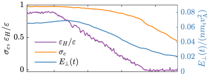
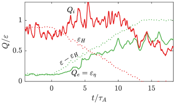
Figure 1: (Top) Time evolution of $\varepsilon_{H}/\varepsilon$ (purple), energy imbalance $\sigma_{c}$ (orange), and total fluctuation energy per unit volume $E_{\perp}(t)$ (blue). (Bottom) Electron heating rate $Q_{e}=\varepsilon_{\eta}$ (green) and ion heating rate $Q_{i}$ (red), with simple helicity-barrier expectations based on the forcing shown with dotted lines.

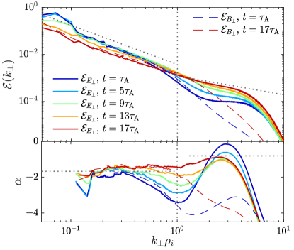
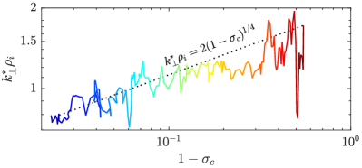
Figure 2: (Top) Perpendicular spectra of the electric field ($\mathcal{E}_{E_{\perp}}$; solid lines) and magnetic field ($\mathcal{E}_{B_{\perp}}$; dashed lines) at a selection of times. The sub-panel illustrates the local spectral slopes $\alpha$, computed via a fit over range $\pm\log_{10}(k_{\perp})\approx 0.1$ around each point; the dotted lines indicate $k_{\perp}\rho_{i}=1$ and the representative power laws $k_{\perp}^{-5/3}$ and $k_{\perp}^{-0.8}$. (Bottom) Evolution of the break scale $k_{\perp}^{*}$ with imbalance $1-\sigma_{c}$, with the line color indicating the time as in the top panel. The dotted line shows the empirical scaling $k_{\perp}^{*}\rho_{i}=2(1-\sigma_{c})^{1/4}$, which provides a good fit to the simulation until $t\approx 11\tau_{\rm A}$.

3.1 Evolution of the helicity barrier

The time evolution as the injection imbalance decreases is shown in Fig. 1. Properties of the saturated imbalanced turbulence, from which the system is initialized, are discussed in S+22; a portion of this phase is shown at $t<0$ for comparison. The imbalance of the fluctuations,

$$\sigma_{c}\equiv\frac{\langle|\bm{z}^{+}|^{2}\rangle-\langle|\bm{z}^{-}|^{2}\rangle}{\langle|\bm{z}^{+}|^{2}\rangle+\langle|\bm{z}^{-}|^{2}\rangle}=\frac{2\langle\bm{u}_{\perp}\,\mbox{\boldmath{$\cdot$}}\,\bm{b}_{\perp}\rangle}{\langle|\bm{u}_{\perp}|^{2}\rangle+\langle|\bm{b}_{\perp}|^{2}\rangle},$$ (4)

starts at $\sigma_{c}\approx 0.98$ for $t<0$, then decreases as the system adjusts to the changing forcing ($\varepsilon_{H}/\varepsilon$). We halt the simulation once $\sigma_{c}\simeq 0.4$, a value similar to that in the solar wind around $1~{}{\rm au}$; as shown below, the heating properties have changed significantly by this point even though $\sigma_{c}$ is still nonzero. The blue line shows the fluctuation energy density $E_{\perp}=\langle nm_{i}(|\bm{u}_{\perp}|^{2}+|\bm{b}_{\perp}|^{2})\rangle/2$, which decreases over the simulation, as expected because the turbulence can dissipate more effectively at lower $\varepsilon_{H}/\varepsilon$.

The lower panel of Fig. 1 compares the measured heating rates, $Q_{i}$ and $\varepsilon_{\eta}$, to helicity-barrier predictions. Here $\varepsilon_{\eta}$, the hyper-resistive dissipation, is taken as a proxy for the electron-heating rate $Q_{e}$, which assumes that ions cannot interact with $k_{\perp}\rho_{i}\gg 1$ eddies and that there is minimal electron heating via ICWs or other $k_{\perp}\rho_{i}\lesssim 1$ fields (Chandran et al., 2010b). For most of the simulation, $\varepsilon_{\eta}$ (green line) tracks well the helicity-barrier prediction $Q_{e}=\varepsilon-\varepsilon_{H}$ (dotted-green line), aside from a delay of ${\sim}\tau_{\rm A}$ as the injected energy cascades towards smaller scales. $Q_{i}$ increases initially because the energy $E_{\perp}(t)$ decreases while the sub-$\rho_{i}$ energy flux is fixed by the helicity barrier. Its large value results from the unrealistically fast decrease of $\varepsilon_{H}/\varepsilon$: in reality $E_{\perp}(t)$ would change more slowly, implying that $Q_{i}=\varepsilon-Q_{e}-\partial_{t}E_{\perp}\approx\varepsilon_{H}-\partial_{t}E_{\perp}$ should more closely track $\varepsilon_{H}$. As $\varepsilon_{H}/\varepsilon$ nears zero ($t/\tau_{\rm A}\gtrsim 10$) and the helicity barrier erodes, the heating departs from $Q_{e}\approx\varepsilon-\varepsilon_{H}$ and approaches that found in kinetic simulations of balanced turbulence at $\beta\approx 0.3$ (Kawazura et al., 2019; Cerri et al., 2021), in which ion heating via Landau damping and stochastic heating absorbs a portion of the energy flux before it reaches the smallest scales. At around the same time, $Q_{i}$ drops significantly.

Figure 2 shows the evolution of the perpendicular spectra $\mathcal{E}(k_{\perp})$ of $\bm{E}_{\perp}$ and $\bm{B}_{\perp}$. The flatter sub-$\rho_{i}$ range in the former helps to highlight the double-kinked “transition-range” power law; for $k_{\perp}\rho_{i}\lesssim 1.5$, including in the transition range, $\mathcal{E}_{E_{\perp}}\approx\mathcal{E}_{B_{\perp}}$. As the turbulence becomes balanced, the spectral break smoothly moves towards smaller scales, creating a less pronounced transition range that is narrower in $k_{\perp}$ and less steep, eventually transitioning directly into the kinetic range with $\mathcal{E}_{E_{\perp}}\sim k_{\perp}^{-0.8}$. At late times, $\delta B_{\perp}$ is resistively damped by the larger resistivity and the magnetic spectrum does not exhibit a clear ${\sim}k_{\perp}^{-2.8}$ kinetic range.

The lower panel of Fig. 2 provides the evolution of the break scale $k^{*}_{\perp}$, obtained by fitting a broken power-law to $\mathcal{E}_{B_{\perp}}(k_{\perp})$. We find a clear power-law dependence on the energy imbalance, $k_{\perp}^{*}\rho_{i}\propto(1-\sigma_{c})^{1/4}\sim(z^{-}_{\rm rms}/z^{+}_{\rm rms})^{1/2}$, for $\sigma_{c}\gtrsim 0.8$ ($t\lesssim 11\tau_{\rm A}$) when the barrier is active ($\varepsilon_{H}/\varepsilon\gtrsim 0$). Although this scaling remains unexplained theoretically, it matches the results of low-$\beta$ gyrokinetic simulations for various choices of $\varepsilon_{H}/\varepsilon$ (Meyrand et al. 2021, figure 7), suggesting it is a robust consequence of the helicity barrier and independent of the energy-dissipation mechanism (gyrokinetics is ignorant of ICW kinetic physics). The persistence of the transition-range drop, as well as the evolution of $\varepsilon_{\eta}$ and $Q_{i}$ in Fig. 2, provide good evidence that a helicity barrier actively mediates the turbulence until $t\approx 11\tau_{\rm A}$, at which point it transitions towards the balanced regime.

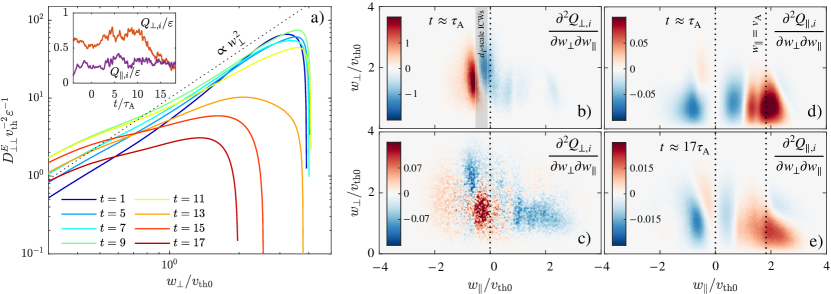
Figure 3: (Left) Time evolution of the perpendicular diffusion energy coefficient $D_{\perp\perp}^{E}$, showing the transition from the quasi-linear expectation $D_{\perp\perp}^{E}\propto w_{\perp}^{2}$ to a flatter profile around $t\gtrsim 11\tau_{\rm A}$. The inset shows the normalized perpendicular (orange) and parallel (purple) ion heating rates, illustrating a sharp drop in $Q_{\perp,i}$ associated with the change in $D_{\perp\perp}^{E}$, while $Q_{\|,i}$ remains almost constant. (Right) Differential heating rates, $v_{\rm th0}^{2}\varepsilon^{-1}\partial^{2}Q_{\perp,\|,i}/\partial w_{\perp}\partial w_{\|}$, computed from $\langle\mbox{\boldmath{$E$}}_{\perp,\|}\,\mbox{\boldmath{$\cdot$}}\,\mbox{\boldmath{$w$}}_{\perp,\|}\rangle$. The $Q_{\perp}$ profile (panels b and c) exhibits resonant structure at early times (top); the shaded region shows $w_{\|{\rm res}}$ for oblique ICWs with $d_{i}^{-1}<k_{\|}<2d_{i}^{-1}$, around where there is a sharp dropoff in wave power (Fig. 4). By late times it drops significantly and an ill-defined peak around $w_{\perp}\simeq v_{\rm th}$ appears, reminiscent of stochastic heating. The $Q_{\|}$ profile (panels d and e) maintains its structure, although spreads out modestly (accounting partially for its lower values).

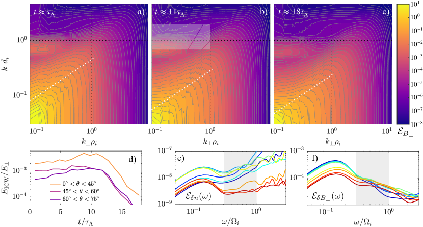
Figure 4: (a)–(c) 2D spectra of $\delta B_{\perp}$, $\mathcal{E}_{B_{\perp}}(k_{\perp},k_{\|})$, at $t\approx\tau_{\rm A}$ (left), $t\approx 11\tau_{\rm A}$ (around the time of the heating transition; middle), and $t\approx 18\tau_{\rm A}$ (right). The dotted white lines show the critical-balance condition $k_{\|}v_{\rm A}=2k_{\perp}z^{+}_{\rm rms}(k_{\perp}/k_{\perp 0})^{-1/3}$. (d) $E_{\rm ICW}$ for different ICW obliquities, which is the energy contained in the shaded regions of panel (b) (see text). (e)–(f) Frequency spectra at different times, using the same colors as Fig. 3a. A sharp drop in high-frequency $\delta n$ fluctuations, taken as a signature of oblique ICW activity, matches the drop in $D_{\perp\perp}^{E}$. In contrast, $\delta B_{\perp}$ fluctuations, present in both parallel and oblique ICWs, drop less abruptly and at later times.

3.2 Consequences for ion heating

This drop in ion heating associated with the balanced transition is diagnosed in Fig. 3. We show the perpendicular energy-diffusion coefficient $D_{\perp\perp}^{E}$ (panel a), which is computed from the measured evolution of $f_{i}$ via

$$D_{\perp\perp}^{E}=\left(\frac{\partial f_{i}}{\partial e_{\perp}}\right)^{-1}\int_{0}^{e_{\perp}}{\rm d}e_{\perp}^{\prime}\frac{\partial f_{i}(e_{\perp}^{\prime})}{\partial t},$$ (5)

where $e_{\perp}\equiv w_{\perp}^{2}/2$ and $f_{i}(e_{\perp})=\int{\rm d}w_{\|}w_{\perp}\,f_{i}(w_{\perp},w_{\|})$. Equation (5) is taken directly from the $D_{\perp\perp}^{E}$ definition, $\partial f_{i}/\partial t=\partial/\partial e_{\perp}(D_{\perp\perp}^{E}\partial f_{i}/\partial e_{\perp})$ (Vasquez et al., 2020), averaging over the $w_{\|}$ variation of $f_{i}$ and assuming that the heating is predominantly perpendicular, as appropriate for $t\lesssim 12\tau_{\rm A}$ (Fig. 3a inset). In quasi-linear theory, waves strongly scatter “resonant” particles with $w_{\|}=w_{\|{\rm res}}\equiv\omega(\bm{k})/k_{\|}-n\Omega_{i}/k_{\|}$ for $n\in\mathbb{Z}$, flattening $f_{i}$ along contours of constant energy in the wave’s frame (the “resonance contours”; we consider only $n=1$ resonances). When parallel waves dominate the spectrum, $D_{\perp\perp}^{E}\propto w_{\perp}^{2}$, because $w_{\|{\rm res}}$ and various wave-intensity/polarization factors are all independent of $w_{\perp}$ (Kennel & Engelmann, 1966). Although the wave spectrum here is more complex, involving a mix of oblique and parallel ICW modes (see below), this prediction is nonetheless well satisfied until $t\approx 11\tau_{\rm A}$. After this, $D_{\perp\perp}^{E}$ drops and flattens, causing a large drop in the perpendicular ion heating $Q_{\perp,i}$, even while the parallel heating $Q_{\|,i}$ remains almost constant (see inset). At later times, the form of $D_{\perp\perp}^{E}$ does not clearly indicate a particular heating mechanism, but is plausibly consistent with stochastic heating (Chandran et al., 2010a): computing the $D_{\perp\perp}^{E}$ predicted for stochastic heating using the method of Cerri et al. (2021) gives a similar shape (not shown). As a complementary analysis, panels (b) and (c) display $\partial^{2}Q_{\perp,i}/\partial w_{\perp}\partial w_{\|}$, the differential perpendicular heating per unit velocity, which is computed directly from $\langle\bm{E}_{\perp}\,\mbox{\boldmath{$\cdot$}}\,\bm{w}_{\perp}\rangle$ evaluated along particle trajectories (the so-called field-particle correlation technique; Klein & Howes, 2016; Arzamasskiy et al., 2019). At early times a resonant feature is centered around the $w_{\|}$ that resonates with the smallest-($d_{i}$)-scale oblique ICWs with significant power (the shaded region shows $w_{\|{\rm res}}$ for $d_{i}^{-1}\lesssim k_{\|}\lesssim 2d_{i}^{-1}$; see Fig. 4); at later times, the magnitude drops significantly into a diffuse peak around $w_{\perp}\simeq v_{\rm th}$, consistent with stochastic heating. In contrast, $\partial^{2}Q_{\|,i}/\partial w_{\perp}\partial w_{\|}$ (the differential parallel heating; panels d and e), maintains a form consistent with Landau damping of kinetic Alfvén waves (KAWs) throughout the simulation.

In Fig. 4 we provide evidence that the shut off in ion heating occurs because the turbulence amplitude decreases to the point where it can no longer drive quasi-linear heating by oblique ICWs. In the top panels, we show 2D spectra of $\delta B_{\perp}$ fluctuations, $\mathcal{E}_{B_{\perp}}(k_{\perp},k_{\|})$, which are computed by filtering each field into $k_{\perp}$ bins, then interpolating these onto the exact magnetic-field lines to take a $k_{\|}$ spectrum (see Methods in S+22). Energy is concentrated at $k_{\perp}>k_{\|}$ (the turbulence) and in a bump at $k_{\perp}\ll k_{\|}\simeq 0.8d_{i}$ (parallel ICWs). Examining the time evolution from left to right, we see that the energy migrates to lower $k_{\|}$ with time (it moves downwards), with the dotted white lines indicating how this follows the critical-balance scaling $k_{\|}v_{\rm A}=Ak_{\perp}z^{+}_{\rm rms}(k_{\perp}/k_{\perp 0})^{-1/3}$ (the coefficient $A=2$ is chosen to align with the “peak” on the cone and is consistent across time). A corollary is that larger-amplitude turbulence feeds more power into smaller-$k_{\|}$ oblique ICWs with smaller $w_{\|{\rm res}}$, driving more quasi-linear heating.

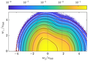
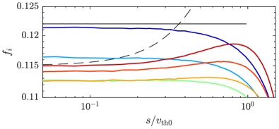
Figure 5: (Top) Contours of the ion VDF $f_{i}$ at $t\approx 5\tau_{\rm A}$ (white lines and colormap) and the $t\approx 18\tau_{\rm A}$ (red lines). Dotted vertical lines highlight $w_{\|}=0$ and $w_{\|}=v_{\rm A}$. The red contour levels are chosen to emphasize changes in $f_{i}$ and do not correspond to the white contours (see text). (Bottom) $f_{i}$ versus distance $s$ along the oblique-ICW resonant contour shown with the black line in the top panel ($s=0$ at $w_{\|}=0$). Colors are as in Fig. 3a. The thin-black line is flat ($\mathcal{G}_{\rm res}[f_{i}]=0$), while the dashed line shows an $f_{i}$ that is independent of $w_{\perp}$ (as expected from stochastic heating).

We quantify this effect in panel (d) by computing the energy of ICWs ($E_{\rm ICW}$), defined as fluctuations with $0.7\leq k_{\|}d_{i}\leq 2$, as a function of wavevector obliquity $\theta=\tan^{-1}(k_{\perp}/k_{z})$. The minimum wavenumber $k_{\|}d_{i}=0.7$ is chosen to capture fluctuations with $w_{\|{\rm res}}\lesssim v_{\rm th}$, which interact with the VDF core (Isenberg & Vasquez, 2011), while the angle ranges capture quasi-parallel ($0<\theta<45^{\circ}$), moderately oblique ($45^{\circ}<\theta<60^{\circ}$), and highly oblique ($60^{\circ}<\theta<75^{\circ}$) populations; these ranges are indicated by the shaded regions in panel (b). Despite $E_{\perp}$ decreasing continuously, the energies of the oblique-ICW populations increase slightly for $t\lesssim 12\tau_{\rm A}$ before dropping rapidly. The similarity of this functional form with that of $Q_{\perp,i}(t)$ provides good evidence for oblique ICWs being the primary driver of heating. The energy of parallel ICWs ($\theta\lesssim 45^{\circ}$) follows a similar trend, but they are not driven directly by the turbulence, which has little power at $k_{\|}\gtrsim k_{\perp}$. Instead they arise because oblique-ICW quasi-linear heating causes $f_{i}$ to increase along the resonance contours of parallel ICWs, thus emitting waves (causing instability; Kennel & Wong, 1967; Chandran et al., 2010b). Their energy is driven and undamped, building up substantially for $t\lesssim 12\tau_{\rm A}$, then decreasing at later times as $f_{i}$ changes shape and renders parallel ICWs stable. Further evidence for this scenario is presented in panels (e) and (f), which show frequency spectra $\mathcal{E}(\omega)$ of the fluctuations in density $\delta n$ (e) and $\delta B_{\perp}$ (f), computed from high-cadence time data at $100$ points, windowed around different times matching Fig. 3 (we highlight the ICW frequency range where $k_{\|}d_{i}\gtrsim 0.7$, $0.3\lesssim\omega/\Omega_{i}\lesssim 1$). While both parallel and oblique ICWs involve $\delta B_{\perp}$ fluctuations, only oblique modes involve $\delta n$. Indeed, we see a significant drop in $\mathcal{E}_{\delta n}$ at the same time as the drop in $Q_{\perp}$, while $\mathcal{E}_{\delta B_{\perp}}$ drops more smoothly and only for $t\gtrsim 13\tau_{\rm A}$ (orange to red lines). The behavior of $\mathcal{E}_{\delta B_{\perp}}$ is consistent with the $0<\theta\leq 45^{\circ}$ $E_{\rm ICW}$ line in panel (d), which only drops below its initial value at $t\approx 13.5\tau_{\rm A}$.

The interpretation described above predicts that $Q_{i}$ scales with the oblique-ICW power, which itself scales with $k_{\|,{\rm max}}d_{i}$, where $k_{\|,{\rm max}}$ corresponds to the smallest parallel scale accessible by the imbalanced portion of the cascade. An independent estimate of $k_{\|,{\rm max}}d_{i}$ can be obtained from the spectrum using $k_{\|,{\rm max}}v_{\rm A}\sim k_{\perp}^{*}z^{+}_{\rm rms}(k_{\perp}^{*}/k_{\perp 0})^{-1/3}$, where $k_{\perp}^{*}\rho_{i}\propto(z^{-}_{\rm rms}/z^{+}_{\rm rms})^{1/2}$ is the break scale (Fig. 2). This gives $k_{\|,{\rm max}}d_{i}\propto\beta^{-1/2}(k_{\perp 0}\rho_{i})^{1/3}(z^{+}_{\rm rms})^{2/3}(z^{-}_{\rm rms})^{1/3}/v_{\rm A}$. In the simulation, $(z^{+}_{\rm rms})^{2}z^{-}_{\rm rms}$ increases modestly for $t\lesssim 11\tau_{\rm A}$ before dropping significantly (not shown), remaining well correlated with $Q_{i}$ and $E_{\rm ICW}$ at all times, including during pre-saturated phase of S+22. This agreement demonstrates the internal consistency of the results across diverse diagnostics ($E_{\rm ICW}$, $Q_{i}$, and $k_{\perp}^{*}$ via $\mathcal{E}_{B_{\perp}}(k_{\perp})$), and could prove useful for developing a closure model for helicity-barrier-mediated turbulence.

The effect of these dynamics on $f_{i}$ is illustrated in Fig. 5, whose top panel superimposes isocontours of $f_{i}(w_{\perp},w_{\|})$ at $t\approx 18\tau_{\rm A}$ over $f_{i}(w_{\perp},w_{\|})$ at $t\approx 5\tau_{\rm A}$. Particles are scattered to render $f_{i}$ constant along the resonant contours, which are computed from $\mathcal{G}_{\rm res}[f_{i}]=0$, where $\mathcal{G}_{\rm res}\equiv(1-w_{\|}/v_{\rm ph})\partial/\partial w_{\perp}+(w_{\perp}/v_{\rm ph})\partial/\partial w_{\|}$ with $v_{\rm ph}(w_{\|})=\omega/k_{\|}$ for resonant waves that satisfy $\omega/k_{\|}-\Omega_{i}/k_{\|}=w_{\|}$. With heating being driven by oblique ICWs but exciting parallel ICWs for $t\lesssim 11\tau_{\rm A}$, we expect $f_{i}$ to decrease along the oblique-ICW contours (which approximately satisfy the $\sin\theta\approx 1$ cold-plasma relation $\omega=k_{\|}v_{\rm A}/\sqrt{1+k_{\|}^{2}d_{i}^{2}}$; Stix, 1992) and to increase along the parallel-ICW contours ($\omega=k_{\|}v_{\rm A}\sqrt{1-\omega/\Omega_{i}}$; see Isenberg 2012 for further discussion of cold-plasma relations in this context). Its evolution towards a flatter core at $t\gtrsim 11\tau_{\rm A}$ is hard to discern on $f_{i}(w_{\perp},w_{\|})$, so in the lower panel we plot $f_{i}$ along an oblique-ICW resonant contour (thin black line). It changes from decreasing slightly to increasing along the contour, with the latter a signature of $f_{i}(w_{\perp},w_{\|})$ becoming flatter in $w_{\perp}$, likely due to stochastic heating (a $w_{\perp}$-independent $f_{i}$ is shown with the dashed line; Klein & Chandran, 2016; Cerri et al., 2021). Various other modifications to $f_{i}$ over the simulation are clear in the top panel, including the smoothing of the sharp “ridge” bordering the quasi-linearly heated region of phase space at $w_{\|}/v_{\rm th0}\approx-0.5$, and the flattening of $f_{i}(w_{\perp})$ at $w_{\|}>0$.

Another feature of $f_{i}$ is the strong parallel plateau, or beam, which results from the Landau damping of $k_{\perp}\gg k_{\|}$ fluctuations at $k_{\perp}\rho_{i}\lesssim 1$ (see also S+22; Li et al. 2010). Such fluctuations, which lie in the $k_{\perp}$ range between Alfvén waves and KAWs, propagate with phase speed ${>}v_{\rm A}$ (Howes et al., 2006), growing a modestly super-Alfvénic plateau in $f_{i}$. As the turbulence becomes balanced, such fluctuations would likely flatten $f_{i}$ at $w_{\|}\approx-v_{\rm A}$ also (see figure 7 of Arzamasskiy et al. 2019), but this feature is not yet observable. The total parallel heating $Q_{\|,i}$, which captures this beam formation, remains almost constant throughout the full simulation (Fig. 3a inset). This suggests that the $k_{\perp}\rho_{i}\sim 1$ Alfvénic fluctuations are Landau damping some fixed portion of their energy before dissipating into oblique ICWs (at earlier times) or KAW turbulence (at later times). A corollary is that there is no fundamental difference between beam formation and standard resonant parallel heating, aside from the fluctuations’ imbalance.

4 Discussion

A complete theory for the helicity barrier would be able to predict the parameters ($\varepsilon_{H}/\varepsilon$, $\beta$, etc.) at which it is operative. Low-$\beta$ gyrokinetics states only that the barrier occurs unless the generalized helicity can be destroyed at least as fast as ${\sim}\varepsilon_{H}$ before $k_{\perp}\rho_{i}\sim 1$ scales are reached (Meyrand et al., 2021). Although generalized helicity is not a true invariant of hybrid kinetics, we can infer from our simulation, based on the agreement between $Q_{e}$ and $\varepsilon-\varepsilon_{H}$ (Fig. 1) and the continuous evolution of the transition-range spectrum (Fig. 2) for $t\lesssim 11\tau_{\rm A}$, that the critical $\varepsilon_{H}/\varepsilon$ at $\beta\approx 0.4$ is ${\approx}0.2$. The changes that occur once $\varepsilon_{H}/\varepsilon\lesssim 0.2$ also coincide with the sharp drop in $Q_{\perp,i}$ (Fig. 3), suggesting that breaking the helicity barrier curtails ion heating. These results highlight the surprising robustness of the helicity barrier in the face of the additional complexities of a true kinetic system. However, $\varepsilon_{H}/\varepsilon$ decreases unrealistically fast in our simulation; understanding how the barrier evolves when $\varepsilon_{H}/\varepsilon$ changes on timescales comparable to the turbulent decay time should be a priority for future work.

Our results provide a helpful roadmap for understanding the radially dependent interplay between turbulence, heating, and instabilities in the $\beta\lesssim 1$ solar wind. At smaller $R$ and in faster streams, which have higher observed imbalance, we predict strong perpendicular ion heating via quasi-linear resonance, continual emission (instability) of parallel ICWs, a steep and wide ion-Larmor-scale transition range, proton beam formation, and little electron heating. At larger $R$ and in slower streams, which have lower imbalance ($\sigma_{c}\lesssim 0.8$ in our simulation), electron heating dominates, parallel ICWs are absorbed/damped, there is no transition-range spectrum, and sharp features in the VDF are smoothed out. These correlations and features match those measured in the low-$\beta$ solar wind by in situ spacecraft (e.g., Marsch, 2006; Bruno et al., 2014; Zhao et al., 2021; Shi et al., 2023).

Under the assumption that, far from the Sun, faster wind is heated more than slower wind (Hansteen & Leer, 1995; Totten et al., 1995; Halekas et al., 2023), our results explain qualitatively various interesting properties of observed temperature profiles. Close to the Sun, proton and minor-ion temperatures correlate positively with wind speed (Burlaga & Ogilvie, 1973), while the electron temperature is negatively correlated (Marsch et al., 1989); this is natural if the highly imbalanced turbulence of faster streams has low $Q_{e}/Q_{i}$ (Shi et al., 2023). At larger distances (${\sim}1~{}{\rm au}$), the electron-temperature correlation flips to positive for $U\lesssim 500~{}{\rm km~{}s}^{-1}$ (Shi et al., 2023), as would occur if $Q_{e}/Q_{i}$ increased to ${\gtrsim}1$ as the turbulence becomes balanced at larger radii. More directly, Abraham et al. (2022) measure $Q_{e}\propto R^{-2}$ for $R\lesssim 0.3~{}{\rm au}$, followed by a rapid drop in $Q_{e}$ at larger $R$. This profile, $Q_{e}\propto R^{-2}$, is much flatter than the “standard” total-heating profile $Q\propto R^{-4}$ (e.g., Totten et al., 1995)—a natural explanation is that $Q=Q_{i}+Q_{e}$ is steeper than $Q_{e}$, because $Q_{e}/Q_{i}$ increases as $\varepsilon_{H}/\varepsilon$ decreases with $R$. Then, once $\varepsilon_{H}/\varepsilon\ll 1$ (around $R\simeq 0.3$ in this scenario), $Q_{e}/Q_{i}$ saturates and $Q_{e}$ drops rapidly.

Together, these observations suggest that imbalanced turbulence and the helicity barrier are actively shaping global coronal and solar-wind dynamics. More generally, they highlight the crucial role of imbalance in controlling collisionless plasma thermodynamics.

We thank S. S. Cerri, C. H. K. Chen, B. D. G. Chandran, E. Quataert, and A. A. Schekochihin for useful discussions. JS and RM acknowledge the support of the Royal Society Te Apārangi, through Marsden-Fund grants MFP-UOO2221 (JS) and MFP U0020 (RM), as well as through the Rutherford Discovery Fellowship RDF-U001804 (JS). This research was part of the Frontera computing project at the Texas Advanced Computing Center, which is made possible by National Science Foundation award OAC-1818253. Further computational support was provided by the New Zealand eScience Infrastructure (NeSI) high performance computing facilities, funded jointly by NeSI’s collaborator institutions and through the NZ MBIE, and through PICSciE-OIT TIGRESS High Performance Computing Center and Visualization Laboratory at Princeton University.

References

- Abraham et al. (2022) Abraham, J. B., Verscharen, D., Wicks, R. T., et al. 2022, Astrophys. J., 941, 145, doi: 10.3847/1538-4357/ac9fd8
- Arzamasskiy et al. (2019) Arzamasskiy, L., Kunz, M. W., Chandran, B. D. G., & Quataert, E. 2019, Astrophys. J., 879, 53, doi: 10.3847/1538-4357/ab20cc
- Arzamasskiy et al. (2023) Arzamasskiy, L., Kunz, M. W., Squire, J., Quataert, E., & Schekochihin, A. A. 2023, Phys. Rev. X, 13, 021014, doi: 10.1103/PhysRevX.13.021014
- Bale et al. (2019) Bale, S. D., Badman, S. T., Bonnell, J. W., et al. 2019, Nature, 576, 237, doi: 10.1038/s41586-019-1818-7
- Bandyopadhyay et al. (2023) Bandyopadhyay, R., Meyer, C. M., Matthaeus, W. H., et al. 2023, Astrophys. J. Lett., 955, L28, doi: 10.3847/2041-8213/acf85e
- Bowen et al. (2022) Bowen, T. A., Chandran, B. D. G., Squire, J., et al. 2022, Phys. Rev. Lett., 129, 165101, doi: 10.1103/PhysRevLett.129.165101
- Bowen et al. (2023) Bowen, T. A., Bale, S. D., Chandran, B. D. G., et al. 2023, arXiv:2306.04881, doi: 10.48550/arXiv.2306.04881
- Bruno & Carbone (2013) Bruno, R., & Carbone, V. 2013, Living Rev. Solar Phys., 10, 2, doi: 10.12942/lrsp-2013-2
- Bruno et al. (2014) Bruno, R., Trenchi, L., & Telloni, D. 2014, Astrophys. J. Lett., 793, L15, doi: 10.1088/2041-8205/793/1/L15
- Burlaga & Ogilvie (1973) Burlaga, L. F., & Ogilvie, K. W. 1973, J. Geophys. Res., 78, 2028, doi: 10.1029/JA078i013p02028
- Cerri et al. (2021) Cerri, S. S., Arzamasskiy, L., & Kunz, M. W. 2021, Astrophys. J., 916, 120, doi: 10.3847/1538-4357/abfbde
- Chandran et al. (2010a) Chandran, B. D. G., Li, B., Rogers, B. N., Quataert, E., & Germaschewski, K. 2010a, Astrophys. J., 720, 503, doi: 10.1088/0004-637X/720/1/503
- Chandran et al. (2010b) Chandran, B. D. G., Pongkitiwanichakul, P., Isenberg, P. A., et al. 2010b, Astrophys. J., 722, 710, doi: 10.1088/0004-637X/722/1/710
- Chen et al. (2016) Chen, C. H. K., Matteini, L., Schekochihin, A. A., et al. 2016, Astrophys. J., 825, 1, doi: 10.3847/2041-8205/825/2/l26
- D’Amicis et al. (2021) D’Amicis, R., Alielden, K., Perrone, D., et al. 2021, Astron. Astro., 654, A111, doi: 10.1051/0004-6361/202140600
- Dobrowolny et al. (1980) Dobrowolny, M., Mangeney, A., & Veltri, P. 1980, Phys. Rev. Lett., 45, 144, doi: 10.1103/PhysRevLett.45.144
- Duan et al. (2021) Duan, D., He, J., Bowen, T. A., et al. 2021, Astrophys. J. Lett., 915, L8, doi: 10.3847/2041-8213/ac07ac
- Fjørtoft (1953) Fjørtoft, R. 1953, Tellus, 5, 225
- Halekas et al. (2023) Halekas, J. S., Bale, S. D., Berthomier, M., et al. 2023, arXiv:2305.13424, doi: 10.48550/arXiv.2305.13424
- Hansteen & Leer (1995) Hansteen, V. H., & Leer, E. 1995, J. Geophys. Res., 100, 21577, doi: 10.1029/95JA02300
- Horbury et al. (2012) Horbury, T. S., Wicks, R. T., & Chen, C. H. K. 2012, Space Sci. Rev., 172, 325, doi: 10.1007/s11214-011-9821-9
- Howes et al. (2006) Howes, G. G., Cowley, S. C., Dorland, W., et al. 2006, Astrophys. J., 651, 590, doi: 10.1086/506172
- Isenberg (2012) Isenberg, P. A. 2012, Phys. Plasmas, 19, 032116, doi: 10.1063/1.3697721
- Isenberg & Vasquez (2011) Isenberg, P. A., & Vasquez, B. J. 2011, Astrophys. J., 731, 88, doi: 10.1088/0004-637X/731/2/88
- Kawazura et al. (2019) Kawazura, Y., Barnes, M., & Schekochihin, A. A. 2019, Proc. Nat. Acad. Sci., 116, 771, doi: 10.1073/pnas.1812491116
- Kennel & Engelmann (1966) Kennel, C. F., & Engelmann, F. 1966, Phys. Fluids, 9, 2377, doi: 10.1063/1.1761629
- Kennel & Wong (1967) Kennel, C. F., & Wong, H. V. 1967, J. Plasma Phys., 1, 75, doi: 10.1017/S002237780000310X
- Klein & Chandran (2016) Klein, K. G., & Chandran, B. D. G. 2016, Astrophys. J., 820, 47, doi: 10.3847/0004-637X/820/1/47
- Klein & Howes (2016) Klein, K. G., & Howes, G. G. 2016, Astrophys. J. Lett., 826, L30, doi: 10.3847/2041-8205/826/2/L30
- Kunz et al. (2014) Kunz, M. W., Stone, J. M., & Bai, X.-N. 2014, J. Comp. Phys., 259, 154, doi: 10.1016/j.jcp.2013.11.035
- Li et al. (1999) Li, X., Habbal, S. R., Hollweg, J. V., & Esser, R. 1999, J. Geophys. Res., 104, 2521, doi: 10.1029/1998JA900126
- Li et al. (2010) Li, X., Lu, Q., Chen, Y., Li, B., & Xia, L. 2010, Astrophys. J. Lett., 719, L190, doi: 10.1088/2041-8205/719/2/L190
- Marsch (2006) Marsch, E. 2006, Living Rev. Solar Phys., 3, 1, doi: 10.12942/lrsp-2006-1
- Marsch et al. (1989) Marsch, E., Pilipp, W. G., Thieme, K. M., & Rosenbauer, H. 1989, J. Geophys. Res., 94, 6893, doi: 10.1029/JA094iA06p06893
- Meyrand et al. (2023) Meyrand, R., Squire, J., Mallet, A., & Chandran, B. D. G. 2023, arXiv:2308.10389, doi: 10.48550/arXiv.2308.10389
- Meyrand et al. (2021) Meyrand, R., Squire, J., Schekochihin, A. A., & Dorland, W. 2021, J. Plasma Phys., 87, 535870301, doi: 10.1017/S0022377821000489
- Parker (1965) Parker, E. N. 1965, Space Sci. Rev., 4, 666, doi: 10.1007/BF00216273
- Roberts et al. (1987) Roberts, D. A., Goldstein, M. L., Klein, L. W., & Matthaeus, W. H. 1987, J. Geophys. Res., 92, 12023, doi: 10.1029/JA092iA11p12023
- Schekochihin (2022) Schekochihin, A. A. 2022, J. Plasma Phys., 88, 155880501. https://arxiv.org/abs/2010.00699
- Schekochihin et al. (2019) Schekochihin, A. A., Kawazura, Y., & Barnes, M. A. 2019, J. Plasma Phys., 85, 905850303, doi: 10.1017/S0022377819000345
- Shi et al. (2023) Shi, C., Velli, M., Lionello, R., et al. 2023, Astrophys. J., 944, 82, doi: 10.3847/1538-4357/acb341
- Squire et al. (2022) Squire, J., Meyrand, R., Kunz, M. W., et al. 2022, Nature Astron., 6, 715, doi: 10.1038/s41550-022-01624-z
- Stix (1992) Stix, T. H. 1992, Waves in plasmas (American Institute of Physics, Melville, NY)
- Totten et al. (1995) Totten, T. L., Freeman, J. W., & Arya, S. 1995, J. Geophys. Res., 100, 13, doi: 10.1029/94JA02420
- Vasquez et al. (2020) Vasquez, B. J., Isenberg, P. A., & Markovskii, S. A. 2020, Astrophys. J., 893, 71, doi: 10.3847/1538-4357/ab7e2b
- Zhao et al. (2021) Zhao, G. Q., Lin, Y., Wang, X. Y., et al. 2021, Astrophys. J., 906, 123, doi: 10.3847/1538-4357/abca3b