Federated Learning of Causal Effects from Incomplete Observational Data

Abstract

Decentralized and incomplete data sources are prevalent in real-world applications, posing a formidable challenge for causal inference. These sources cannot be consolidated into a single entity owing to privacy constraints, and the presence of missing values within them can potentially introduce bias to the causal estimands. We introduce a new approach for federated causal inference from incomplete data, enabling the estimation of causal effects from multiple decentralized and incomplete data sources. Our approach disentangles the loss function into multiple components, each corresponding to a specific data source with missing values. Our approach accounts for the missing data under the missing at random assumption, while also estimating higher-order statistics of the causal estimands. Our method recovers the conditional distribution of missing confounders given the observed confounders from the decentralized data sources to identify causal effects. Our framework estimates heterogeneous causal effects without the sharing of raw training data among sources, which helps to mitigate privacy risks. The efficacy of our approach is demonstrated through a collection of simulated and real-world instances, illustrating its potential and practicality.

1 Introduction

Causal inferences are important in real-life applications: What is the impact of a new drug on patient survival? How do vaccination campaigns help reduce the incidence and spread of infectious diseases? What are the impacts of social and public policies across various domains such as poverty alleviation, education reform, and labor market interventions? To accurately estimate causal effects from observational data, a large amount of experimental or observational data is often required, which may contain missing values and be distributed across different sources. Missing data attributed to a multitude of reasons such as erroneous data entry or processing, data loss, data deletion, etc, and it is commonly appeared in real-life application (Allison,, 2001; Baraldi and Enders,, 2010; Cismondi et al.,, 2013). Dealing with missing data is crucial for accurate estimation of causal effects as it might introduce biases and result in misleading conclusions. Data curation and maintenance across multiple sources, such as patient data from various hospitals, can be complex. However, combining these sources for processing can be challenging due to organizational or policy constraints. For instance, some countries have strict confidentiality regulations for medical or health records, particularly those related to cancer patients. These real-world scenarios pose a significant research question: How can a causal model be learned to estimate causal effects across multiple data sources, accounting for missing data, while simultaneously minimizing the potential risks associated with compromising data records’ confidentiality and sensitivity?

Most current methods for causal inference (e.g., Hill,, 2011; Shalit et al.,, 2017; Louizos et al.,, 2017; Künzel et al.,, 2019; Nie and Wager,, 2021) mainly focus on estimating causal effects from a single and complete data source. They require data to be centralized in a single machine, violating the privacy constraints of the data, and are unable to handle missing data. Using a separate method to impute missing data might introduce bias based on the chosen imputation method. Only a few recent works (e.g., Vo et al., 2022b, ; Vo et al., 2022a, ; Xiong et al.,, 2021) have proposed federated methods to estimate causal effects from multiple data sources. However, these methods also cannot handle data sources that contain missing values. On the other hand, methods that estimate causal effects in the presence of missing data (e.g., Crowe et al.,, 2010; Mitra and Reiter,, 2011; Seaman and White,, 2014; Yang et al.,, 2019; Hillis et al.,, 2021) are not designed within the context of a federated setting, where data needs to be on the same machine for performing inference. The main research question, therefore, is how to securely access these diverse data sources and handle missing data in order to construct an effective global causal effect estimator, all while carefully managing the risk of compromising data privacy and confidentiality.

In this work, we propose a novel Bayesian method for conducting federated causal inference on incomplete/missing data that is spread across multiple decentralized and heterogeneously distributed sources. Our method can estimate higher-order statistics of the causal estimands, thereby capturing their uncertainty. Our contributions are as follows:

• We propose a new method called CausalFI (Causal Federated inference on Incomplete data), which recovers the distribution of missing confounders conditioned on the observed ones. This enables estimating causal effects from multiple data sources with missing values.

• We conduct federated causal inference with CausalFI using data from multiple sources with missing data. The inference is carried out without sharing raw data among the sources, thereby minimizing the risk of a privacy breach.

• We empirically assess the performance of the proposed framework on benchmark datasets and demonstrate its competitiveness compared to recent baseline approaches.

2 Background and Related Work

The integration of privacy-preserving federated learning, causal inference methods, and handling missing data remains relatively unexplored in the literature.

Causal inference from observational data: This problem poses a significant challenge due to the limitations of conducting the gold standard randomized controlled trials (RCTs). The feasibility and ethical considerations often restrict RCTs’ applicability. Consequently, primary problem in causal inference from observational data lies in effectively addressing confounders (also known as confounding variables), which represent common causes influencing both the treatment and the outcome variables. Confounders are pivotal to accurately estimate reliable causal estimands in observational studies. Most popular methods (e.g., Hill,, 2011; Alaa and van der Schaar,, 2017, 2018; Shalit et al.,, 2017; Yoon et al.,, 2018; Yao et al.,, 2018; Künzel et al.,, 2019; Nie and Wager,, 2021) assumed all confounders are observed, and they adopted the standard strong ignorability, and Stable Unit Treatment Value Assumption (SUTVA) (Rosenbaum and Rubin,, 1983) to learn causal effects directly from local observational data sources. Louizos et al., (2017); Madras et al., (2019); Vo et al., 2022a considered latent confounders and they adapted the structural causal model (SCM) of Pearl, (1995) to estimate the causal effects by leveraging additional proxy variables to infer the latent confounders. These methods, except Vo et al., 2022a , cannot perform causal inference from multiple and decentralised sources that cannot be combined in a central machine for processing. They also failed to learn causal effects on data sources that contain missing values.

Federated learning for causal inference: Federated learning is a framework that learns a shared prediction model while maintaining the decentralized nature of the training data across multiple sources (McMahan et al.,, 2017). Little research was proposed for the federated estimation of causal effects. Vo et al., 2022b proposed a Gaussian processes-based method that estimates posterior distributions of causal effects and hence capturing uncertainty of the causal estimands. Vo et al., 2022a estimated causal effects from multiple sources whose data distributions might be dissimilar. Xiong et al., (2021) estimated average treatment effect (ATE) and average treatment effect on the treated (ATT) and assumed that the confounders are observed. All these works do not take into account missing data. On the other hand, our work estimates conditional average treatment effect (CATE) and ATE with existence of missing confounders. Considering missing data in real-life applications is vital to mitigate biases, enhance generalizability, improve statistical efficiency, and derive more accurate and reliable conclusions.

Causal inference and missing data mechanism: The commonly recognized types of missing data mechanisms (Rubin,, 1976) include: missing completely at random (MCAR), missing at random (MAR), and missing not at Random (MNAR). Qu and Lipkovich, (2009); Crowe et al., (2010); Mitra and Reiter, (2011); Seaman and White, (2014); Kallus et al., (2018); Yang et al., (2019); Mayer et al., 2020a ; Mayer et al., 2020b ; Hillis et al., (2021) are typical works that consider estimating causal effects in the present of missing data. Yang et al., (2019) assumed MNAR and outcome-independent of the missing indicators to derive a non-parametric method for estimating causal effects. Hillis et al., (2021) introduce a missing data mechanism that integrates with an iterative multivariate matching method, leveraging random forest to construct a distance matrix, and then facilitating subsequent optimal matching. Qu and Lipkovich, (2009); Crowe et al., (2010); Mitra and Reiter, (2011); Seaman and White, (2014) proposed multiple imputation-based methods based on MCAR or MAR assumptions for imputing the missing values, consequently estimating propensity score for estimation of ATE. Mayer et al., 2020b proposed a doubly robust estimator to estimate ATE and ATT with missing attributes. These methods, however, required data to be centralized in a central client, which might breaches the confidential and private information. Our approach is distinct in that it does not rely on an outcome-independent assumption and instead focuses on estimating causal effects without the need to aggregate raw data.

3 The Proposed Model

In this section, we first describe the problem setting of federated causal inference from missing data. We then state necessary assumptions for identification of causal effects and propose CausalFI, a Bayesian federated estimator, that learns distributions of the causal estimands.

3.1 Problem Setting

Consider a scenario of estimating causal effects of a treatment on an outcome. Let $W\in\{0,1\}$ be binary treatment. Let $Y_{0}$ and $Y_{1}$ be two potential outcomes associated with $W=0$ and $W=1$, respectively. Let $Y$ be observed outcome, then we have the following relations: $Y=(1-W)\cdot Y_{0}+W\cdot Y_{1}$. This is also known as the consistency assumption in causal inference, i.e., the factual outcome $Y$ equals to the potential outcome $Y_{0}$ when $W=0$, and $Y_{1}$ when $W=1$. Let $X$ and $Z$ be two sets of confounders where $X$ is always observed and $Z$ is partially observed, i.e., there are missing values in $Z$. The number of dimensions of $Z$ is $d$. Let $R=[R_{1},\!...R_{d}]$ be vector of missing indicators for $Z$, i.e., $Z_{i}$ is missing/unknown if $R_{i}=0$ and $Z_{i}$ is observed if $R_{i}=1$.

Suppose we have $m$ data sources, each locally curated and organized, denoted as $D^{\mathsf{s}}=\{(w_{i}^{\mathsf{s}},y_{i}^{\mathsf{s}},x_{i}^{\mathsf{s}},z_{i}^{\mathsf{s}},r_{i}^{\mathsf{s}})\}_{i=1}^{n_{\mathsf{s}}}$, where $\mathsf{s}\in[m]$ (i.e., $\mathsf{s}\in\{1,\!...,m\}$). Here, $w_{i}^{\mathsf{s}}$, $y_{i}^{\mathsf{s}}$, $x_{i}^{\mathsf{s}}$, $z_{i}^{\mathsf{s}}$, and $r_{i}^{\mathsf{s}}$ represent realization samples of the treatment assignment, observed outcome, observed confounders, partially observed confounders, and missing indicator for individual $i$ in source $\mathsf{s}$, i.e., they are realization values of the random variables $W$, $Y$, $X$, $Z$, and $R$. We aim to utilize all $m$ data sources to learn a causal model without combining or sharing raw data among the sources, and at the same time learning higher order statistic of the causal estimands. In the subsequent section, we state some necessary assumptions required to estimate causal effects in a federated setting with missing data.

3.2 Causal Quantities of Interest & Assumptions

Let $r$ be a specific missing pattern, i.e., it is a realization value of the random vector variable $R$. We further denote $Z_{r}$ and $Z_{\tilde{r}}$ as sets of observed and missing variables in $Z$, i.e., $Z=\{Z_{r},Z_{\tilde{r}}\}$. We would like to estimate conditional average treatment effect (CATE) and average treatment effect (ATE) which are defined as follows:

$$\tau(x,z_{r})=E\big{[}Y_{1}-Y_{0}|X=x,Z_{r}=z_{r}\big{]},\qquad\qquad\tau=E\big{[}Y_{1}-Y_{0}\big{]},$$ (1)

where $\tau(x,z_{r})$ is the average treatment affect conditioned on the observed confounders $X=x$ and $Z_{r}=z_{r}$. Herein, the confounder $z_{\tilde{r}}$ is missing (or unknown). To estimate causal effects from multiple observational data sources, we first make some assumptions:

Assumption 1 (Strong ignorability).

($i$) The potential outcomes are independent of the treatment assignment conditional on the covariates (unconfoundedness), i.e., $Y_{1},Y_{0}\!\perp\!\!\!\perp\!W|X,Z$, and ($ii$) every individual has some positive probability to be assigned to every treatment (positivity), i.e., $0<\text{Pr}(W\!=\!1|X,Z)<1$. (Rosenbaum and Rubin,, 1983)

Assumption 2 (SUTVA).

($i$) The potential outcomes for any individual do not vary with the treatments assigned to other individuals, and ($ii$) there are no different forms or versions of each treatment level, which would lead to different potential outcomes. (Imbens and Rubin,, 2015)

Assumptions 1 and 2 would allow the causal quantities in Eq. (1) to be written in terms of the observed outcome $Y$. However, since the confounder $Z$ is partially observed, further assumptions are required.

Assumption 3 (MCAR and MAR).

($i$) Missing indicators might depend on the observed confounders, treatment assignments, and observed outcomes, and ($ii$) they are independent of the incomplete confounders given all the observed variables, i.e., $R_{i}\perp\!\!\!\perp Z_{j}|X,Y,W$ for all $i,j\in[d]$.

Assumption 4.

$\text{Pr}(R_{i}=1|X,Y,W)>c$ for $i\in[d]$.

Assumptions 1–4 would allow the causal effects to be estimated from missing observational data. The following assumptions are made to enable federated causal estimations:

Assumption 5.

The individuals from all sources share the same set of common covariates.

Assumption 6.

There exists a ‘set of primary features’ that enables the unique identification of any individual across different data sources.

Assumption 5 is reasonable for federated learning, such as those observed in Choudhury et al., (2019); Vaid et al., (2020); Flores et al., (2021). In Assumption 6, a ‘set of primary features’ need not be limited to the observed data used for inference, and could include additional features that can uniquely identify an individual, e.g., their nationality or national identification number. Assumption 6 further permits a secure preprocessing procedure to eliminate repeated individual records across different sources, if required, without sharing raw data (Vo et al., 2022a, ; Vo et al., 2022b, ).

3.3 Identification of Causal Effects with Missing Observational Data

In this section, we discuss identifiability of $\tau$ and $\tau(x,z_{r})$. From Eq. (1), we would need to estimate $\psi_{w}:=E[Y_{w}]$ and $\psi_{w}(x,z_{r}):=E[Y_{w}|X=x,Z_{r}=z_{r}]$, for $w\in\{0,1\}$. Hence, we have:

$$\tau(x,z_{r})=\psi_{1}(x,z_{r})-\psi_{0}(x,z_{r}),\qquad\tau=\psi_{1}-\psi_{0}.$$

Under Assumptions 1 and 2, we can rewrite $\psi_{w}$ and $\psi_{w}(x,z_{r})$ as follows:

$$\psi_{w}(x,z_{r}) =E_{Z_{\tilde{r}}}\big{[}E_{Y}[Y|W=w,X=x,Z_{r}=z_{r},Z_{\tilde{r}}]\big{]},$$ (2)

$$\psi_{w} =E_{X,Z_{r}}\big{[}\psi_{w}(X,Z_{r})\big{]},$$ (3)

where the inner expectation of $\psi_{w}(x,z_{r})$ is taken over $p(y|w,x,z_{r},z_{\tilde{r}})=p(y|w,x,z)$, and the outer expectation is taken over $p(z_{\tilde{r}}|x,z_{r})$.

Imputation might be a biased estimator: Now we show that using imputation and then apply a typical causal inference method might introduce bias. Let $z_{\tilde{r}}^{\ast}$ be imputed value of $z_{\tilde{r}}$. Then, the estimate of $\psi_{w}(x,z_{r})$ is:

$$\hat{\psi}_{w}(x,z_{r},z_{r}^{\ast})=E_{Y}\!\big{[}Y|W=w,X=x,Z_{r}=z_{r},Z_{\tilde{r}}=z_{\tilde{r}}^{\ast}\big{]}.$$ (4)

Generally, our objective is to ensure that $z_{r}^{\ast}$ satisfies the condition $\hat{\psi}_{w}(x,z_{r},z_{r}^{\ast})=\psi_{w}(x,z_{r})$. However, achieving this alignment might pose certain challenges.

Lemma 1.

Let $z_{\tilde{r}}^{\ast}$ be imputed value by regression, and let $g(z_{\tilde{r}})=E[Y|W\!=\!w,X\!=\!x,Z_{r}\!=\!z_{r},Z_{\tilde{r}}\!=\!z_{\tilde{r}}]$. We have:

1. If $g(z_{\tilde{r}})$ is non-linear, then $\psi_{w}(x,z_{r})\neq\hat{\psi}_{w}(x,z_{r},z_{r}^{\ast})$.

2. If $g(z_{\tilde{r}})$ is linear, then $\psi_{w}(x,z_{r})=\hat{\psi}_{w}(x,z_{r},z_{r}^{\ast})$.

Lemma 1 indicates that constructing a regression-based imputation approach to forecast a missing value $z_{\tilde{r}}^{\ast}$, while conditioning on observed variables $X=x$ and $Z_{z}=z_{r}$, is only viable when the outcome is a linear function of the confounders. It could potentially introduce bias into causal estimations when the outcome is a non-linear function of the confounders containing missing values. Yet, in practical scenarios, the inherent nature of the function $g(z_{\tilde{r}})$ remains uncertain–whether it adheres to linearity or exhibits non-linear characteristics.

The proposed procedure: We now explain our approach where we learn a distribution of the missing values rather than a fixed point. To estimate $\psi_{w}(x,z_{r})$ and $\psi_{w}$, we need to draw samples of $Z_{\tilde{r}}$ from

$$p(z_{\tilde{r}}|x,z_{r})\propto p(z|x)$$ (5)

and samples of $Y$ from $p(y|w,x,z)$. Hence, the key is to learn $p(y|w,x,z)$ and $p(z|x)$ from the multiple data sources. However, learning these two distributions is challenging since $Z$ is missing according to the indicator vector $R$. Only using observed records in the dataset to learn these distributions is biased since $p(y|w,x,z)\neq p(y|r=1,w,x,z)$ and $p(z|x)\neq p(z|r=1,x)$. So we need to take into account the missing data while performing inference. We have that

$$p(y|w,x,z)\propto p(z|y,w,x)p(y,w,x),$$ (6)

$$p(z|x)=\sum_{w}\int p(z|y,w,x)p(y,w,x)dy.$$ (7)

Eq. (7) implies that $p(y|w,x,z)$ and $p(z|x)$ are identifiable if $p(z|y,w,x)$ and $p(y,w,x)$ are identifiable. Since $Y$, $W$, and $X$ are all fully observed variables, $p(y,w,x)$ is identifiable. From Assumption 3, we have that $p(z|y,w,x)=p(z|r=1,y,w,x)$, which enable the learning of $p(z|y,w,x)$ from the observed records data. Assumption 4 ensures that there exists observed records in the multiple sources data for performing inference. Once $p(z|y,w,x)$ and $p(y|w,x)$ are identified, a naive approach to estimate $\psi_{w}$ and $\psi_{w}(x,z_{r})$ is to draw samples of $Z_{\tilde{r}}$ and $Y$ from $p(z_{\tilde{r}}|x,z_{r})$ and $p(y|w,x,z)$ using Markov Chain Monte Carlo or inverse transform sampling depending on whether the variables are continuous or discrete. Although this is a possible approach, drawing samples of $Z_{\tilde{r}}$ and $Y$ using the relation in Eq. (5) and (7) might face a numerical issue since we need to integrate and sum over $y$ and $w$. Hence, we propose two surrogate $\hat{p}(z_{\tilde{r}}|x,z_{r})$ and $\hat{p}(y|w,x,z)$ that are learned from the pseudo data points of $Z$ drawn from $p(z|y,w,x)$. To obtain the pseudo points, we can use forward sampling by drawing samples $(y,w,x)$ from the observed dataset and then using them as given values in $p(z|y,w,x)$ to draw samples for $Z$.

To summarize, we would need to learn $p(z|y,w,x)$, and the two surrogate $\hat{p}(z_{\tilde{r}}|x,z_{r})$, $\hat{p}(y|w,x,z)$. In the subsequent section, we propose a federated learning approach to learn these distribution from multiple data sources.

3.4 CausalFI: Federated Causal Inference from Incomplete Data

In this section, present a Bayesian federated approach to estimate causal effects from multiple data sources.

Learning $p(z|y,w,x)$: We parameterize different model depending on each dimension of $Z$. Let $p(z;\Lambda)$ be probability density/mass function of $Z$, where $\Lambda$ is the set of parameters of the density. For example, if $p(z;\Lambda)$ is density of a Gaussian distribution, then $\Lambda$ is a set of the mean and variance. To model the conditional distribution $p(z|y,w,x)$, we set

$$\lambda:=\lambda(\theta^{\lambda})=wf_{1}^{\lambda}(y,x;\theta_{1}^{\lambda})+(1-w)f_{0}^{\lambda}(y,x;\theta_{0}^{\lambda})$$ (8)

for $\lambda\in\Lambda$, where $\theta_{0}^{\lambda}$ and $\theta_{1}^{\lambda}$ be sets of parameters modelling $\lambda$ when $w=0$ and $w=1$, respectively.

Let $\theta=\bigcup_{\lambda\in\Lambda}\{\theta_{0}^{\lambda},\theta_{1}^{\lambda}\}$ be set of all parameters. To capture higher-order statistic of the causal estimands in a Bayesian setting, we learn the posterior distribution $p(\theta|\mathbf{y},\mathbf{w},\mathbf{x})$, where $\mathbf{y},\mathbf{w},\mathbf{x}$ are observational data from all sources. This would required data to be collected to a central machine to compute the posterior, which violates the federated setting. To overcome this problem, we use a variational approximation which would learn a set of shared variational parameters among the sources and avoid sharing raw data among them. To proceed, we specify a variational posterior distribution $q_{\phi}(\theta)$ and learn its sets of parameters $\phi$ by maximizing the evidence lower bound:

$$L=\sum_{\mathsf{s}=1}^{m}L^{\mathsf{s}},\qquad\qquad L^{\mathsf{s}}=E_{\theta}\big{[}\log p(\mathbf{z}_{r}^{\mathsf{s}}|\mathbf{y}^{\mathsf{s}},\mathbf{w}^{\mathsf{s}},\mathbf{x}^{\mathsf{s}};\theta)\big{]}-m^{-1}D_{\text{KL}}[q_{\phi}(\theta)\|p(\theta)],$$ (9)

where $\mathbf{z}_{r}^{\mathsf{s}},\mathbf{y}^{\mathsf{s}},\mathbf{w}^{\mathsf{s}},\mathbf{x}^{\mathsf{s}}$ are observational data in source $\mathsf{s}$, and $p(\theta)$ is a prior distribution. The objective function $L$ is decomposed to multiple components $L^{\mathsf{s}}$, each associated with a data sources. So we can maximize it in a federated setting by aggregating either the local models or the gradients. The conditional log-likelihood $\log p(\mathbf{z}_{r}^{\mathsf{s}}|\mathbf{y}^{\mathsf{s}},\mathbf{w}^{\mathsf{s}},\mathbf{x}^{\mathsf{s}};\theta)$ depends on the domain of $Z$, e.g., for continuous variable, the conditional log-likelihood is in the form of squared error; for binary or categorical, it is cross-entropy; for count variable, it is log of probability mass function of Poisson distribution or Negative binomial distribution. We learn $p(z|y,w,x)$ by maximizing the objective functions in the form of Eq. (9). We obtain its variational posterior denoted by $q_{\phi_{z}}(\theta_{z})$. The variational posterior would enable calculating higher-order statistic of the causal estimands.

Learning $\hat{p}(z_{\tilde{r}}|x,z_{r})$ and $\hat{p}(y|w,x,z)$: To estimate CATE, it is crucial to sample the missing confounder $z_{\tilde{r}}$ from $p(z_{\tilde{r}}|x,z_{r})$ and then sample the outcome from $p(y|w,x,z)$. This can be achieved by utilizing Markov Chain Monte Carlo (MCMC) methods. However, this is not a wise solution since identification of $p(z_{\tilde{r}}|x,z_{r})$ requires marginalization over $w$ and $y$ as shown in Eq. (5) and (7), and there is no analytical solution for this marginalization. We overcome this problem by proposing surrogate models $\hat{p}(z_{\tilde{r}}|x,z_{r};\theta_{z})$, $\hat{p}(y|w,x,z;\theta_{y})$, and we learn variational distributions $q_{\hat{\phi}}(\theta_{z})$, $q_{\hat{\phi}}(\theta_{y})$, in federated setting. This model is learned from the pseudo data points of $z$ generated from $p(z|y,w,x)$ through Eq. (7) with forward sampling. The loss functions for learning these two distributions are similar to that of Eq. (9).

Algorithm 1 Federated calculation of ATE and CATE

Input: $D^{{}^{\prime}\mathsf{s}}\!=\!\{(x_{i}^{{}^{\prime}\mathsf{s}},z_{i}^{{}^{\prime}\mathsf{s}},r_{i}^{{}^{\prime}\mathsf{s}})\!:\!i\!\in\![n_{\mathsf{s}}^{\prime}]\}$ for $\mathsf{s}\in[m^{\prime}]$

1:  In the server machine:

2:         Draw $\{\theta_{z}^{(k)}\}_{k=1}^{K}\sim q_{\hat{\phi}}(\theta_{z})$ and $\{\theta_{y}^{(k)}\}_{k=1}^{K}\sim q_{\hat{\phi}}(\theta_{y})$

3:         Send $\{(\theta_{z}^{(k)},\theta_{y}^{(k)})\}_{k=1}^{K}$ to all sources.

4:  In each source machine $\mathsf{s}\in[m^{\prime}]$:

5:         Call Algorithm 2 to obtain $\mathcal{A}_{1}^{\mathsf{s}}\!\vcentcolon=\!\{\widehat{\text{ATE}}_{k}^{\mathsf{s}}\!:\!k\!\in\![K]\}$, and $\mathcal{A}_{2}^{\mathsf{s}}\vcentcolon=\{\widehat{\text{CATE}}_{ik}\!:\!i\!\in\![n_{\mathsf{s}}^{\prime}],k\!\in\![K]\}$.

6:         Compute CATE and its higher-order statistics for each individual $i$ in source $\mathsf{s}$ using $\mathcal{A}_{2}^{\mathsf{s}}$.

7:         Send $\mathcal{A}_{1}^{\mathsf{s}}$ to the server machine.

8:  In the server machine:

9:         Compute $\widehat{\text{ATE}}_{k}=(\sum_{\mathsf{s}=1}^{m^{\prime}}n_{\mathsf{s}}^{\prime}\widehat{\text{ATE}}_{k}^{\mathsf{s}})/\sum_{\mathsf{s}=1}^{m^{\prime}}n_{\mathsf{s}}^{\prime}$

10:         Compute ATE and its higher-order statistics from $\{\widehat{\text{ATE}}_{k}:k\in[K]\}$.

Algorithm 2 Samples of ATE and CATE on local source $\mathsf{s}$

Input: $D^{{}^{\prime}\mathsf{s}}\!=\!\{(x_{i}^{{}^{\prime}\mathsf{s}},z_{i}^{{}^{\prime}\mathsf{s}},r_{i}^{{}^{\prime}\mathsf{s}})\!:\!i\!\in\![n_{\mathsf{s}}^{\prime}]\}$, $\{(\theta_{z}^{(k)},\theta_{y}^{(k)})\!:\!k\!\in\![K]\}$
Output: Samples of ATE^s and CATE for each $(\theta_{z}^{(k)},\theta_{y}^{(k)})$.

1:  for $k=1$ to $K$ do

2:     for $i=1$ to $n_{\mathsf{s}}^{\prime}$ do

3:        Let $(x^{\prime},z^{\prime},r^{\prime})=(x_{i}^{{}^{\prime}\mathsf{s}},z_{i}^{{}^{\prime}\mathsf{s}},r_{i}^{{}^{\prime}\mathsf{s}})$

4:        Draw $\{z^{\prime}_{\tilde{r^{\prime}}}(j)\}_{j=1}^{N}\!\sim\!\hat{p}(z^{\prime}_{\tilde{r^{\prime}}}|x^{\prime},z^{\prime}_{r^{\prime}};\theta_{z}^{(k)})$

5:        for $j=1$ to $N$ do

6:           Let $z^{\prime}_{j}=(z^{\prime}_{r^{\prime}},z^{\prime}_{\tilde{r^{\prime}}}(j))$

7:           Draw $\{y^{\prime}_{0jl}\}_{l=1}^{M}\sim\hat{p}(y^{\prime}|w=0,x^{\prime},z^{\prime}_{j};\theta_{y}^{(k)})$

8:           Draw $\{y^{\prime}_{1jl}\}_{l=1}^{M}\sim\hat{p}(y^{\prime}|w=1,x^{\prime},z^{\prime}_{j};\theta_{y}^{(k)})$

9:        $\widehat{\text{CATE}}_{ik}\!=\!\sum_{j=1}^{N}\sum_{l=1}^{M}(y^{\prime}_{1jl}-y^{\prime}_{0jl})/(MN)$

10:     $\widehat{\text{ATE}}_{k}^{\mathsf{s}}=\sum_{i=1}^{n_{\mathsf{s}}^{\prime}}\widehat{\text{CATE}}_{ik}/n_{\mathsf{s}}^{\prime}$

11:  return $\{\widehat{\text{ATE}}_{k}^{\mathsf{s}}\!:\!k\!\in\![K]\}$, $\{\widehat{\text{CATE}}_{ik}\!:\!i\!\in\![n_{\mathsf{s}}^{\prime}],k\!\in\![K]\}$

3.5 Estimating Causal Effects

Given a set of new data points in $m^{\prime}$ sources ($m^{\prime}\leq m)$: $D^{{}^{\prime}\mathsf{s}}=\{(x_{i}^{{}^{\prime}\mathsf{s}},z_{i}^{{}^{\prime}\mathsf{s}},r_{i}^{{}^{\prime}\mathsf{s}}):i\in[n_{\mathsf{s}}^{\prime}]\}$, where $\mathsf{s}\in[m^{\prime}]$ and $z_{i}^{{}^{\prime}\mathsf{s}}$s might contain missing values, we would like to estimate CATE and ATE. To compute these causal quantities of interest and their higher-order statistics, we draw $K$ samples of $\theta_{z}$ and $\theta_{y}$ from their variational posterior distributions, denoted as $\{(\theta_{z}^{(k)},\theta_{y}^{(k)}):k\in[K]\}$. Each sample $(\theta_{z}^{(k)},\theta_{y}^{(k)})$ is used to compute one sample for ATE and CATE, and there are $K$ samples. We can use these $K$ samples of ATE and CATE to compute their mean, variance, skewness, kurtosis, etc. For each sample $(\theta_{z}^{(k)},\theta_{y}^{(k)})$, we empirically calculate $\psi_{w}(x^{\prime},z^{\prime}_{r^{\prime}})$ and $\psi_{w}$ using Eq. (2) and (3). To proceed, for each given data points $(x^{\prime},z^{\prime},r^{\prime})\in D^{\prime}$, we draw samples of $Z_{\tilde{r}}$ from $\hat{p}(z^{\prime}_{\tilde{r^{\prime}}}|x^{\prime},z^{\prime}_{r^{\prime}};\theta_{z}^{(k)})$. We then substitute the above samples to $\hat{p}(y^{\prime}|w^{\prime},x^{\prime},z^{\prime};\theta_{y}^{(k)})$ to draw samples of $Y$ and calculate its empirical expectation. The empirical $\psi_{w}$ can be calculated using Eq. (3) by averaging $\psi_{w}(x^{\prime},z^{\prime}_{r^{\prime}})$ over all data points in $\bigcup_{\mathsf{s}=1}^{m^{\prime}}D^{{}^{\prime}\mathsf{s}}$. We summarise the steps of federated estimating causal effects in Algorithm 1 and 2.

3.6 Missing Mechanism Testing

This work assumes MCAR and MAR, and these missing mechanisms are testable. The Little’s test (Little,, 1988) is the well-known test for MCAR. The test is available in software packages like SPSS, SAS, and R. Testing for MAR is more complex as it implies that the missingness is related to the observed data but not the unobserved data. There is no single definitive test for MAR, but several approaches can be used to assess the assumption such as Molenberghs and Kenward, (2007); Little and Rubin, (2019); Enders, (2022). A drawback of existing missing mechanism tests is their inability to assess missing data across multiple data sources in a federated setting. To address this limitation, we present a straightforward approach that involves conducting individual tests on each data source and subsequently determining the prevailing missing data mechanism through a voting method. This allows us to account for the distinct characteristics of each data source while making a collective inference about the missing mechanism. For future research, an interesting topic is to develop federated tests for missing data mechanism.

4 Experiments

Baselines & the aims of experiments. In this section, we first study the performance of CausalFI compared with the cases of bootstrap aggregating and on combined data. We also study its performance on different portion of missing data. We then compare CausalFI with the existing baselines including: BART (Hill,, 2011), TARNet (Shalit et al.,, 2017), CFR-Wass (CFRNet with Wasserstein distance) (Shalit et al.,, 2017), CFR-MMD (CFRNet with maximum mean discrepancy distance) (Shalit et al.,, 2017), CEVAE (Louizos et al.,, 2017), OrthoRF (Oprescu et al.,, 2019), IPW (Seaman and White,, 2014), DR (Mayer et al., 2020b, ), X-learner (Künzel et al.,, 2019), R-learner (Nie and Wager,, 2021), and FedCI (Vo et al., 2022b, ). Note that these methods, except IPW and DR, do not do not directly deal with missing data. Hence, we first impute the missing data and then fit the baselines. We impute with two popular methods: probabilistic principal component analysis (ppca) (Tipping and Bishop,, 1999), and multivariate imputation by chained equations (mice) (Van Buuren and Groothuis-Oudshoorn,, 2011). In addition, for most of the baselines that are not federated methods (BART, TARNet, CFR-wass, CFR-mmd, CEVAE, OrthorRF, X-learner, R-learner), we would train them in two cases: ($i$) using bootstrap aggregating of Breiman, (1996) where $m$ models are trained separately on each source data and then averaging the predicted treatment effects based on each trained model (denoted as avg), ($ii$) training a global model with the combined data from all the sources (denoted as com). Note that case ($ii$) might breach sensitive information, it is only used for the purposes of comparison. In summary, there are four different cases: ppca+avg, ppca+com, mice+avg, and mice+com.

Implementation of the baselines. We reuse source code of the baselines which are publicly available. We train CEVAE using implementation from Louizos et al., (2017). Implementation of TARNet and CFR are from Shalit et al., (2017). For these methods, we use Exponential Linear Unit (ELU) activation function and fine-tune the number of nodes in each hidden later from 10 to 200 with step size of addition by 10. We use package BartPy for BART, and package causalml (Chen et al.,, 2020) for X-learner and R-learner. Experiments on OrthoRF is with the package econml (Microsoft Research,, 2019). Implementation of IPW and DR is from Mayer et al., 2020b . Finally, implementation of FedCI is from Vo et al., 2022b . The learning rate is fine-tuned from $\{10^{-5},10^{-4},10^{-3},10^{-2},10^{-1}\}$ for all methods. For TARNet, CFR-wass, CFR-mmd, OrthoRF, X-learner, R-learner, we additionally fine-tune the regularizer factors in $\{10^{-5},10^{-4},10^{-3},10^{-2},10^{-1},10^{0}\}$. Two error metrics are used to compare the methods: $\epsilon_{\mathrm{PEHE}}$ (precision in estimation of heterogeneous effects) and $\epsilon_{\mathrm{ATE}}$ (absolute error) to compare the methods:

$$\epsilon_{\mathrm{PEHE}} =\sum_{i=1}^{n}(\tau(x_{i},z_{ri})-\hat{\tau}(x_{i},z_{ri}))^{2}/n,$$

$$\epsilon_{\mathrm{ATE}} =|\tau-\hat{\tau}|,$$

where $\uptau(x_{i},z_{ri}),\uptau$ are the ground truth of CATE and ATE, and $\hat{\tau}(x_{i},z_{ri}),\hat{\tau}$ are their estimates.

For comparing the point estimation, we report the mean and standard error of the error metrics over 10 replicates of the data.

4.1 Synthetic Data

To evaluate the performance of CausalFI, we simulate variables with a ground truth model and divide them into multiple sources for federated learning. We use the following ground truth distributions to simulate the data:

$$\bm{u}_{i} \sim\mathsf{N}(\bm{m},\bm{\Sigma}),$$

$$w_{i} \sim\mathsf{Bern}(\mathsf{sig}(a_{0}+\bm{b}_{1}^{\top}\bm{u}_{i})),$$

$$y_{0i} \sim\mathsf{N}(\mathsf{sp}(c_{0}+\bm{c}_{1}^{\top}\bm{u}_{i}),\sigma_{0}^{2}),$$

$$y_{1i} \sim\mathsf{N}(\mathsf{sp}(d_{0}+\bm{d}_{1}^{\top}\bm{u}_{i}),\sigma_{1}^{2}),$$

where $\mathsf{N}(\cdot)$, $\mathsf{Bern}(\cdot)$ denote the Gaussian and Bernoulli distributions, $\mathsf{sig}(\cdot)$ denotes the sigmoid function and $\mathsf{sp}(\cdot)$ is the softplus function. We only keep $y_{i}=w_{i}y_{1i}+(1-w_{i})y_{0i}$ as the observed outcome. The vector $\bm{u}_{i}$ contains all confounders and we split it into two sets $\bm{z}_{i}$ and $\bm{x}_{i}$. $\bm{z}_{i}$ is a vectors that might contain missing values, and $\bm{x}_{i}$ is always observed. We simulate missing indicators for $\bm{z}_{i}$ using:

$$r_{ji}\sim\mathsf{Bern}(\mathsf{sig}(e_{j0}+e_{j1}w_{i}+e_{j2}y_{i}+\bm{e}_{j3}^{\top}\bm{x}_{i})),$$ (10)

for each dimension $j$ of $\bm{z}_{i}$. Herein, $e_{j0}$, $e_{j1}$, $e_{j2}$, $\bm{e}_{j3}$ are the ground truth parameters and they are randomly set. In particular, we set $e_{j0}=5.0$ and randomly draw $e_{j1},e_{j2}\sim\mathsf{U}[-2,0]$, $\bm{e}_{j3}\sim\mathsf{N}(\bm{0},\mathbf{M})$, where $\mathbf{M}=\mathbf{L}\mathbf{L}^{\top}$, $\mathbf{L}\in\mathbb{R}^{10\times 5}$ and each element $L_{ij}\sim\mathsf{U}[0,0.5]$. For each dataset, we simulate 10 replications, each has $10,000$ data points. We randomly divide the data into 50 sources, each has 200 data points. For each data source, we split it into three sets of 100, 50, 50 data points for training, testing, and validation. In Table 1, we report the percentage of missing values of each confounder in the synthetic data. In Table 2, we report the percentage of missing values of each confounder in IHDP data.

Table 1: Percentage of missing entries in each incomplete confounder on synthetic data.

Replicate	$z_{1}$	$z_{2}$	$z_{3}$	$z_{4}$	$z_{5}$	$z_{6}$	$z_{7}$	$z_{8}$	$z_{9}$	$z_{10}$
#1	30%	44%	25%	49%	52	24%	62%	33%	49%	37%
#2	72%	39%	76%	81%	37%	74%	85%	31%	31%	31%
#3	76%	37%	41%	57%	40%	55%	78%	37%	33%	35%
#4	65%	51%	32%	57%	52%	53%	79%	56%	44%	48%
#5	38%	44%	27%	54%	46%	37%	69%	39%	38%	34%
#6	56%	79%	46%	89%	73%	38%	90%	56%	64%	60%
#7	69%	61%	33%	84%	63%	42%	77%	36%	51%	57%
#8	48%	26%	55%	61%	28%	60%	65%	15%	24%	22%
#9	61%	54%	38%	83%	54%	43%	72%	18%	44%	48%
#10	61%	60%	31%	73%	63%	31%	77%	44%	56%	55%

Table 2: Percentage of missing entries in each incomplete confounder on IHDP data.

Replicate	$z_{1}$	$z_{2}$	$z_{3}$	$z_{4}$
#1	20.16%	20.16%	20.83%	20.56%
#2	46.91%	46.64%	46.91%	44.09%
#3	93.01%	93.28%	92.74%	94.09%
#4	44.89%	42.61%	46.24%	45.43%
#5	23.39%	26.08%	25.40%	24.46%
#6	60.62%	60.35%	58.87%	57.12%
#7	28.76%	31.45%	29.84%	29.03%
#8	82.93%	83.20%	82.53%	83.60%
#9	0.13%	0.67%	0.00%	0.27%
#10	15.46%	17.34%	16.80%	17.34%

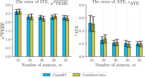
Figure 1: Federated inference analysis on synthetic data.

CausalFI vs. training on combined data: In this experiment, we study the performance of CausalFI compared with the case of combining data. The results in Figure 1 show that the performance of CausalFI is as good as training on combined data as expected. This verifies the efficacy of our proposed federated training method.

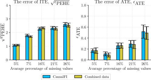
Figure 2: The errors on different number of missing features.

Analysis on learning missing confounders: This experiment aims to learn the performance of CausalFI on different number of missing features. We train the model when there are 2, 4, 6, 8 and 10 incomplete confounders, which are associated with an average of 5%, 7%, 16%, 21%, and 26% missing entries. Herein, we also compare with the case of training on combined data. Figure 2 shows that when there are more confounders that contain missing values, the errors are a bit higher. This result is expected as there are more missing values. Importantly, the errors of CausalFI are as low as those of training on combined data. In addition, we illustrate marginal distributions of the learned pseudo data compared with distributions of the complete data and incomplete data in Figure 3. The figures show that distributions of the learned pseudo data (used by CausalFI) are close to those of complete data. This explains why CausalFI can recover distribution of the missing confounders and hence identifies the causal effects of interest.

Table 3: Out-of-sample errors of CATE and ATE on synthetic data (lower is better). Top-3 performances are highlighted in bold. Settings that violate privacy constraint are highlighted in gray ($\blacksquare$) and they are only used for comparison purpose.

	The error of CATE, $\sqrt{\epsilon_{\text{PEHE}}}$			The error of ATE, $\epsilon_{\text{ATE}}$
# of sources	10 sources	30 sources	50 sources	10 sources	30 sources	50 sources
BART${}_{\text{ppca+com}}$	7.47$\pm$.58	7.45$\pm$.56	7.23$\pm$.59	3.31$\pm$.61	3.34$\pm$.55	3.27$\pm$.56
BART${}_{\text{mice+com}}$	7.43$\pm$.57	7.43$\pm$.57	7.23$\pm$.57	3.22$\pm$.62	3.34$\pm$.60	3.41$\pm$.60
BART${}_{\text{ppca+avg}}$	7.52$\pm$.64	7.55$\pm$.53	7.43$\pm$.52	3.43$\pm$.52	3.51$\pm$.53	3.51$\pm$.61
BART${}_{\text{mice+avg}}$	7.49$\pm$.61	7.51$\pm$.52	7.35$\pm$.47	3.29$\pm$.61	3.49$\pm$.49	3.47$\pm$.58
R-learner${}_{\text{ppaca+com}}$	5.30$\pm$.27	4.65$\pm$.28	4.50$\pm$.31	1.12$\pm$.28	1.19$\pm$.18	1.08$\pm$.23
R-learner${}_{\text{mice+com}}$	5.70$\pm$.30	4.91$\pm$.41	4.53$\pm$.31	1.59$\pm$.33	1.53$\pm$.25	1.40$\pm$.23
R-learner${}_{\text{ppca+avg}}$	7.29$\pm$.59	7.17$\pm$.59	7.22$\pm$.58	2.62$\pm$.74	2.46$\pm$.74	2.49$\pm$.74
R-learner${}_{\text{ppca+avg}}$	7.52$\pm$.51	7.43$\pm$.50	7.37$\pm$.49	2.47$\pm$.72	2.43$\pm$.60	2.41$\pm$.72
X-learner${}_{\text{ppca+com}}$	5.79$\pm$.39	5.61$\pm$.37	5.91$\pm$.42	1.53$\pm$.31	1.70$\pm$.34	2.13$\pm$.34
X-learner${}_{\text{mice+com}}$	5.75$\pm$.35	6.19$\pm$.40	5.98$\pm$.35	2.02$\pm$.32	2.56$\pm$.29	2.52$\pm$.27
X-learner${}_{\text{ppca+avg}}$	5.84$\pm$.38	5.77$\pm$.38	5.81$\pm$.37	1.17$\pm$.29	1.18$\pm$.26	1.22$\pm$.27
X-learner${}_{\text{mice+avg}}$	5.92$\pm$.37	5.64$\pm$.41	5.72$\pm$.38	1.27$\pm$.21	1.21$\pm$.29	1.24$\pm$.25
OthoRF${}_{\text{ppca+com}}$	7.83$\pm$.64	7.72$\pm$.58	7.61$\pm$.57	3.50$\pm$.73	3.37$\pm$.63	2.32$\pm$.60
OthoRF${}_{\text{mice+com}}$	7.95$\pm$.58	7.69$\pm$.53	7.55$\pm$.52	3.34$\pm$.66	3.33$\pm$.58	3.32$\pm$.57
OthoRF${}_{\text{ppca+avg}}$	7.97$\pm$.76	7.55$\pm$.67	6.93$\pm$.62	3.80$\pm$.69	3.21$\pm$.65	2.89$\pm$.50
OthoRF${}_{\text{mice+avg}}$	8.05$\pm$.71	7.61$\pm$.60	6.99$\pm$.61	3.50$\pm$.71	3.32$\pm$.63	2.94$\pm$.52
TARNet${}_{\text{ppca+com}}$	3.63$\pm$.13	3.62$\pm$.15	3.63$\pm$.15	1.38$\pm$.22	1.40$\pm$.32	1.35$\pm$.30
TARNet${}_{\text{mice+com}}$	3.52$\pm$.15	3.48$\pm$.17	3.50$\pm$.18	1.29$\pm$.25	1.34$\pm$.31	1.32$\pm$.30
TARNet${}_{\text{ppca+avg}}$	4.77$\pm$.48	4.51$\pm$.29	4.15$\pm$.61	1.80$\pm$.39	1.76$\pm$.43	1.61$\pm$.39
TARNet${}_{\text{ppca+avg}}$	4.61$\pm$.41	4.47$\pm$.31	4.01$\pm$.55	1.71$\pm$.42	1.61$\pm$.41	1.50$\pm$.37
CFR-mmd${}_{\text{ppca+com}}$	3.72$\pm$.21	3.72$\pm$.20	3.75$\pm$.22	0.83$\pm$.16	0.77$\pm$.15	0.74$\pm$.17
CFR-mmd${}_{\text{mice+com}}$	3.59$\pm$.22	3.59$\pm$.20	3.64$\pm$.22	0.89$\pm$.26	0.89$\pm$.24	0.93$\pm$.27
CFR-mmd${}_{\text{ppca+avg}}$	4.52$\pm$.71	4.22$\pm$.54	4.11$\pm$.63	1.75$\pm$.41	1.71$\pm$.42	1.50$\pm$.29
CFR-mmd${}_{\text{ppca+avg}}$	4.41$\pm$.60	4.11$\pm$.52	3.91$\pm$.61	1.62$\pm$.42	1.50$\pm$.41	1.28$\pm$.34
CFR-wass${}_{\text{ppca+com}}$	3.77$\pm$.16	3.78$\pm$.16	3.77$\pm$.16	1.32$\pm$.27	1.32$\pm$.27	1.30$\pm$.27
CFR-wass${}_{\text{mice+com}}$	3.95$\pm$.14	3.96$\pm$.13	3.96$\pm$.14	1.52$\pm$.29	1.52$\pm$.29	1.51$\pm$.28
CFR-wass${}_{\text{ppca+avg}}$	4.51$\pm$.32	4.12$\pm$.31	4.07$\pm$.25	1.77$\pm$.51	1.68$\pm$.49	1.61$\pm$.39
CFR-wass${}_{\text{mice+avg}}$	4.82$\pm$.35	4.26$\pm$.37	4.11$\pm$.21	1.65$\pm$.53	1.50$\pm$.42	1.53$\pm$.30
CEVAE${}_{\text{ppca+com}}$	3.99$\pm$.31	3.41$\pm$.30	3.48$\pm$.27	1.14$\pm$.31	0.75$\pm$.19	0.85$\pm$.30
CEVAE${}_{\text{mice+com}}$	3.09$\pm$.22	4.45$\pm$.99	3.99$\pm$.62	0.69$\pm$.27	1.37$\pm$.73	1.24$\pm$.48
CEVAE${}_{\text{ppca+avg}}$	4.35$\pm$.38	3.28$\pm$.29	3.34$\pm$.32	1.22$\pm$.45	0.97$\pm$.26	1.01$\pm$.34
CEVAE${}_{\text{mice+avg}}$	4.47$\pm$.40	4.59$\pm$.23	4.24$\pm$.32	1.01$\pm$.41	1.07$\pm$.21	1.18$\pm$.29
FedCI${}_{\text{ppca+com}}$	2.72$\pm$.13	2.52$\pm$.18	2.47$\pm$.17	0.78$\pm$.10	0.57$\pm$.11	0.59$\pm$.11
FedCI${}_{\text{mice+com}}$	2.62$\pm$.13	2.54$\pm$.16	2.52$\pm$.17	0.62$\pm$.15	0.55$\pm$.15	0.52$\pm$.12
FedCI${}_{\text{ppca+avg}}$	3.11$\pm$.17	3.04$\pm$.20	2.98$\pm$.19	0.89$\pm$.12	0.72$\pm$.10	0.69$\pm$.13
FedCI${}_{\text{mice+avg}}$	3.18$\pm$.13	3.10$\pm$.15	3.02$\pm$.16	0.85$\pm$.12	0.70$\pm$.14	0.65$\pm$.12
CausalFI	2.60$\pm$.14	2.28$\pm$.12	2.26$\pm$.12	0.52$\pm$.12	0.21$\pm$.04	0.20$\pm$.03

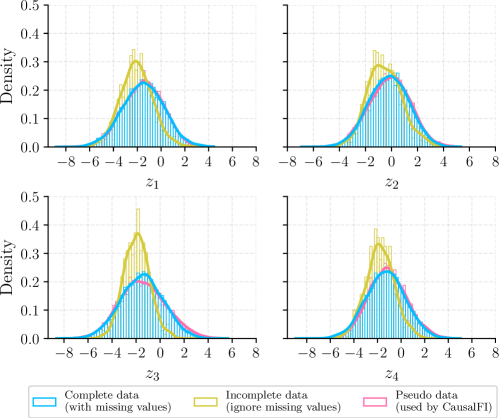
Figure 3: Marginal distribution of $Z_{1},Z_{2},Z_{3},Z_{4}$ pseudo data compared with those of complete and incomplete data.

Compare with baselines: As mentioned earlier, we have four settings for the baselines: ppca+com, mice+com, ppca+avg, mice+avg. For FedCI, since this is a federated method, we only use combined data and bootstrap aggregating when imputing missing values, and the training of FedCI is a federated setting. This experiment is with 10 incomplete confounders (26% of missing values). The results in Table 3 show that CausalFI is among top-3 performance. It achieves lower errors compared to BART, R-learner, X-learner, OthoRF, TARNet, and CFR trained on combined data. In comparison with CEVAE${}_{\text{ppca+com}}$, CEVAE${}_{\text{mice+com}}$, FedCI${}_{\text{ppca+com}}$, and FedCI${}_{\text{mice+com}}$, CausalFI achieves competitive results. However, imputation of the missing values in these four baselines require combining data, which violate federated data setting. In addition, we also observe that performance of the baselines depends on the impute method used. Especially in the case of CEVAE, each imputation method (ppca or mice) would result in a very different error of ATE. Meanwhile, CausalFI learns distributions of the missing confounders while training the model.

For comparison with IPW and DR, these methods are designed for missing data, but they can only estimate in-sample ATE, but not CATE. Hence, we compare with them separately in Table 5. The imputation used in these methods are pca (principal components analysis) and mice. The results show that CausalFI significantly outperform these baselines.

Table 4: In-sample errors of ATE ($\epsilon_{\text{ATE}}$) on synthetic data.

	10 sources	30 sources	50 sources
IPW${}_{\text{pca+com}}$	2.6$\pm$0.9	1.9$\pm$0.7	1.3$\pm$0.4
IPW${}_{\text{mice+com}}$	2.9$\pm$0.3	2.8$\pm$0.2	2.5$\pm$0.2
IPW${}_{\text{com}}$	3.0$\pm$0.4	2.8$\pm$0.3	2.6$\pm$0.2
DR${}_{\text{pca+com}}$	2.8$\pm$0.8	2.4$\pm$0.6	2.2$\pm$0.6
DR${}_{\text{mice+com}}$	3.9$\pm$0.9	3.7$\pm$1.0	3.2$\pm$0.6
DR${}_{\text{com}}$	3.7$\pm$0.8	3.2$\pm$1.0	2.8$\pm$0.5
CausalFI	0.3$\pm$.10	0.2$\pm$.05	0.2$\pm$.04

Table 5: In-sample errors of ATE ($\epsilon_{\text{ATE}}$) on IHDP data.

	2 sources	4 sources	6 sources
IPW${}_{\text{pca+com}}$	1.2$\pm$0.5	0.6$\pm$0.2	0.5$\pm$0.2
IPW${}_{\text{mice+com}}$	1.2$\pm$0.4	0.7$\pm$0.2	0.6$\pm$0.2
IPW${}_{\text{com}}$	0.9$\pm$0.2	0.4$\pm$0.2	0.4$\pm$0.1
DR${}_{\text{pca+com}}$	0.8$\pm$0.3	0.7$\pm$0.3	0.3$\pm$0.1
DR${}_{\text{mice+com}}$	0.8$\pm$0.3	0.5$\pm$0.2	0.2$\pm$0.1
DR${}_{\text{com}}$	1.4$\pm$0.6	0.6$\pm$0.1	0.6$\pm$0.2
CausalFI	1.1$\pm$0.3	0.6$\pm$0.1	0.3$\pm$0.1

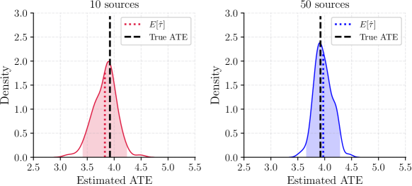
Figure 4: Distribution of the estimated ATE.

Table 6: Standard deviation of CausalFI vs. FedCI.

	10 sources	30 sources	50 sources
FedCI	6.83	6.39	6.16
CausalFI	0.21	0.18	0.16

Distribution of the estimated ATE: We report distributions of the estimated ATE in Figure 4. As expected, the figures show that expectation of the causal estimand shifts toward the true ATE, and the confidence interval shrinks when the model is trained with more sources. It also shows that the true ATE is within the confidence interval, which is helpful for decision making. Note that the standard deviation of CausalFI is smaller than that of FedCI as the distribution in CausalFI is learned from all sources. Meanwhile, standard deviation of FedCI only depends on the number of data points in a single source. This is because FedCI is based on Gaussian Process, and it computes the variance using local training data in a specific source. In Table 6, we report standard deviations of CausalFI and FedCI on different number of sources, which verifies our hypothesis.

4.2 IHDP Data

Data description: We further describe the dataset in this section. The Infant Health and Development Program (IHDP) (Hill,, 2011) contains 744 data points, each consisting of 25 covariates. These data were collected as part of a randomized study investigating the impact of specialist visits on children’s cognitive development. This dataset was ‘de-randomized’ by removing from the treated set children with non-white mothers. In this study, specialist visits represent the treatment, and children’s cognitive development is the outcome of interest. To assess the treatment’s effectiveness, we utilize the NPCI package (Dorie,, 2016) to simulate two potential outcomes for each child, one with specialist visits and one without. By doing so, we can compute the true conditional average treatment effect for evaluation purposes. The dataset is replicated ten times, and each replicate is divided into six subsets, each containing 124 data points. For each of these subsets, we further split them into three sets of 80, 24, and 20 data points for training, testing, and validation purposes when building the models. We then calculate the mean and standard error of the evaluation metrics across these ten replicates of the data. To simulate missing indicators, we also use Eq. (10). We set $e_{j0}=1.0$, $e_{j1}=-0.5$, $e_{j2}=-0.03$, $\bm{e}_{j3}\sim\mathsf{N}(\bm{0},\mathbf{M})$, where $\mathbf{M}=\mathbf{L}\mathbf{L}^{\top}$, $\mathbf{L}\in\mathbb{R}^{21\times 4}$ and each element $L_{ij}\sim\mathsf{U}[0,0.5]$. We use Eq. (10) to simulate missing indicators of 4 incomplete confounders. In Table 2, we report the percentage of missing values of each confounder in IHDP data.

Table 7: Out-of-sample errors of CATE and ATE on IHDP data (lower is better). Top-3 performances are highlighted in bold. Settings that violate privacy constraint are highlighted in gray ($\blacksquare$) and they are only used for comparison purpose.

	The error of CATE, $\sqrt{\epsilon_{\text{PEHE}}}$			The error of ATE, $\epsilon_{\text{ATE}}$
# of sources	2 sources	4 sources	6 sources	2 sources	4 sources	6 sources
BART${}_{\text{ppca+com}}$	5.35$\pm$1.4	5.15$\pm$1.3	4.72$\pm$1.4	1.72$\pm$1.0	0.99$\pm$0.5	0.67$\pm$0.2
BART${}_{\text{mice+com}}$	5.57$\pm$1.3	5.53$\pm$1.6	5.38$\pm$1.2	2.06$\pm$1.1	1.78$\pm$0.7	1.31$\pm$0.5
BART${}_{\text{ppca+avg}}$	5.58$\pm$1.5	5.55$\pm$1.3	5.36$\pm$1.2	2.09$\pm$1.2	1.80$\pm$0.7	1.28$\pm$0.4
BART${}_{\text{mice+avg}}$	5.93$\pm$1.7	5.79$\pm$1.4	5.52$\pm$1.4	2.12$\pm$1.3	1.88$\pm$0.8	1.52$\pm$0.6
R-learner${}_{\text{ppca+com}}$	6.08$\pm$1.7	5.47$\pm$1.8	6.10$\pm$1.5	3.34$\pm$1.2	3.54$\pm$1.3	4.28$\pm$1.4
R-learner${}_{\text{mice+com}}$	5.84$\pm$1.5	5.55$\pm$1.7	5.74$\pm$1.7	3.50$\pm$1.4	3.29$\pm$1.0	3.78$\pm$1.2
R-learner${}_{\text{ppca+avg}}$	6.64$\pm$1.7	5.26$\pm$1.3	5.70$\pm$1.4	3.74$\pm$1.2	2.84$\pm$1.3	3.55$\pm$1.5
R-learner${}_{\text{mice+avg}}$	5.49$\pm$1.6	5.49$\pm$1.4	5.69$\pm$1.3	3.02$\pm$1.2	2.93$\pm$1.1	3.65$\pm$0.9
X-learner${}_{\text{ppca+com}}$	4.04$\pm$1.5	3.57$\pm$1.2	3.20$\pm$0.9	1.06$\pm$0.4	0.90$\pm$0.3	1.02$\pm$0.4
X-learner${}_{\text{mice+com}}$	3.94$\pm$1.5	3.63$\pm$1.2	3.09$\pm$0.9	0.92$\pm$0.3	0.88$\pm$0.3	0.82$\pm$0.3
X-learner${}_{\text{ppca+avg}}$	3.93$\pm$1.5	3.95$\pm$1.6	3.74$\pm$1.4	1.22$\pm$0.6	1.34$\pm$0.6	1.18$\pm$0.5
X-learner${}_{\text{mice+avg}}$	3.97$\pm$1.5	4.05$\pm$1.6	3.85$\pm$1.5	1.33$\pm$0.6	1.29$\pm$0.6	1.13$\pm$0.6
OthoRF${}_{\text{ppca+com}}$	4.31$\pm$1.4	3.73$\pm$1.3	3.11$\pm$1.2	1.38$\pm$0.7	0.99$\pm$0.6	0.70$\pm$0.5
OthoRF${}_{\text{mice+com}}$	4.28$\pm$1.5	3.89$\pm$1.6	3.07$\pm$1.5	1.55$\pm$0.8	1.23$\pm$0.7	0.83$\pm$0.6
OthoRF${}_{\text{ppca+avg}}$	4.77$\pm$1.6	4.10$\pm$1.4	3.62$\pm$1.3	1.47$\pm$0.8	1.28$\pm$0.6	1.11$\pm$0.7
OthoRF${}_{\text{mice+avg}}$	4.65$\pm$1.6	3.98$\pm$1.6	3.37$\pm$1.3	1.68$\pm$0.7	1.41$\pm$0.6	0.98$\pm$0.6
TARNet${}_{\text{ppca+com}}$	5.97$\pm$1.8	5.63$\pm$1.6	4.22$\pm$1.2	2.05$\pm$0.6	1.49$\pm$0.5	0.87$\pm$0.1
TARNet${}_{\text{mice+com}}$	6.53$\pm$1.6	6.25$\pm$1.5	4.36$\pm$1.2	2.04$\pm$0.7	1.90$\pm$0.6	1.03$\pm$0.1
TARNet${}_{\text{ppca+avg}}$	6.05$\pm$1.7	5.96$\pm$1.6	5.31$\pm$1.4	2.11$\pm$0.7	1.65$\pm$0.5	0.92$\pm$0.3
TARNet${}_{\text{ppca+avg}}$	6.96$\pm$1.8	6.45$\pm$1.5	4.91$\pm$1.3	2.34$\pm$0.8	2.04$\pm$0.6	1.14$\pm$0.3
CFR-mmd${}_{\text{ppca+com}}$	5.53$\pm$1.5	6.69$\pm$1.7	5.48$\pm$1.1	1.19$\pm$0.3	1.76$\pm$0.5	1.59$\pm$0.3
CFR-mmd${}_{\text{mice+com}}$	6.20$\pm$1.5	6.39$\pm$1.7	5.58$\pm$1.2	1.58$\pm$0.4	1.88$\pm$0.5	1.81$\pm$0.4
CFR-mmd${}_{\text{ppca+avg}}$	5.78$\pm$1.7	6.82$\pm$1.8	5.63$\pm$1.3	1.31$\pm$0.4	1.81$\pm$0.5	1.63$\pm$0.3
CFR-mmd${}_{\text{ppca+avg}}$	6.67$\pm$1.6	6.52$\pm$1.5	5.76$\pm$1.3	1.61$\pm$0.5	1.91$\pm$0.5	1.89$\pm$0.4
CFR-wass${}_{\text{ppca+com}}$	5.98$\pm$1.7	6.31$\pm$1.5	5.07$\pm$1.2	1.05$\pm$0.3	1.15$\pm$0.3	1.39$\pm$0.3
CFR-wass${}_{\text{mice+com}}$	5.93$\pm$1.7	6.18$\pm$1.6	5.43$\pm$1.4	1.18$\pm$0.3	1.64$\pm$0.5	1.67$\pm$0.7
CFR-wass${}_{\text{ppca+avg}}$	6.21$\pm$1.6	6.53$\pm$1.6	5.31$\pm$1.3	1.21$\pm$0.4	1.21$\pm$0.4	1.46$\pm$0.5
CFR-wass${}_{\text{mice+avg}}$	6.31$\pm$1.7	6.52$\pm$1.8	5.61$\pm$1.3	1.32$\pm$0.5	1.78$\pm$0.5	1.72$\pm$0.6
CEVAE${}_{\text{ppca+com}}$	4.74$\pm$1.5	4.43$\pm$1.4	4.54$\pm$1.5	0.65$\pm$0.2	1.06$\pm$0.3	0.98$\pm$0.3
CEVAE${}_{\text{mice+com}}$	4.82$\pm$1.4	4.41$\pm$1.3	4.63$\pm$1.2	1.03$\pm$0.4	1.21$\pm$0.3	1.02$\pm$0.3
CEVAE${}_{\text{ppca+avg}}$	4.97$\pm$1.6	4.65$\pm$1.3	4.72$\pm$1.1	0.98$\pm$0.4	1.23$\pm$0.4	1.08$\pm$0.3
CEVAE${}_{\text{mice+avg}}$	5.03$\pm$1.6	4.82$\pm$1.4	4.74$\pm$1.2	1.24$\pm$0.7	1.32$\pm$0.3	1.15$\pm$0.3
FedCI${}_{\text{ppca+com}}$	3.97$\pm$1.6	3.52$\pm$1.3	3.15$\pm$1.4	0.98$\pm$0.3	0.78$\pm$0.2	0.61$\pm$0.2
FedCI${}_{\text{mice+com}}$	4.12$\pm$1.7	3.85$\pm$1.4	3.04$\pm$1.2	1.01$\pm$0.4	0.85$\pm$0.3	0.78$\pm$0.2
FedCI${}_{\text{ppca+avg}}$	4.61$\pm$1.7	3.89$\pm$1.5	3.62$\pm$1.3	1.12$\pm$0.3	1.02$\pm$0.2	0.91$\pm$0.2
FedCI${}_{\text{mice+avg}}$	4.45$\pm$1.8	3.91$\pm$1.5	3.52$\pm$1.3	1.17$\pm$0.4	0.92$\pm$0.2	0.89$\pm$0.2
CausalFI	3.67$\pm$1.7	3.33$\pm$1.4	2.99$\pm$1.2	0.73$\pm$0.3	0.53$\pm$0.2	0.32$\pm$0.1

Results and discussion: We report the results in Table 7. Similar to experimental results on synthetic data, the results in this dataset show that the performance of CausalFI is competitive to the baselines. In particular, CausalFI is among top-3 performance. This again verifies the efficacy of the proposed method. We also observe that the errors of CEVAE, CFR-mmd, and CFR-wass in estimating ATE are a bit higher when there are more missing data points. This could be because of the performance of the impute method. We also report comparison with IPW and DR regarding in-sample $\epsilon_{\text{ATE}}$ in Table 5, which shows competitive results. However, these baselines are trained on combined data which violates privacy constraint of the data. Similar to the results on synthetic data, the distribution of ATE on IHDP data are shown in Figure 5. The figures show that the true ATE are within the confidence interval, and the mean of the estimated ATE shifts towards the true ATE when there are more sources. We also compare standard deviation of CausalFI with FedCI in Table 8. The figures show that standard deviation of CausalFI is smaller than that of FedCI, which demonstrates that CausalFI would give a more confident result than FedCI.

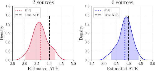
Figure 5: Distribution of the estimated ATE on IHDP data in replicate #1.

Table 8: Standard deviation of CausalFI vs. FedCI on IHDP data.

	2 sources	4 sources	6 sources
FedCI	7.60	7.71	7.47
CausalFI	0.31	0.30	0.28

5 Conclusion

This work presents an approach to address the challenge of federated causal inference from incomplete and decentralized data. It tackles the issue of missing data under MAR and MCAR assumption. We recover the conditional distribution of missing confounders given the observed confounders from the decentralized data sources. Importantly, our method estimates heterogeneous causal effects while ensuring privacy, but not requiring the sharing of raw data. An interesting future research is to extend the proposed causal effect estimator for MNAR and consider different data distributions among the sources. Such scenario might require a transfer learning approach while handling missing data, and further assumptions might be needed for the causal effects to be identifiable. It is important to test for missing data mechanism. At present, the only method is to apply existing tests locally on each source and then aggregate them with a simple voting approach. Another future direction is to develop a federated test for missing data mechanism.

References

- Alaa and van der Schaar, (2018) Alaa, A. and van der Schaar, M. (2018). Limits of estimating heterogeneous treatment effects: Guidelines for practical algorithm design. In International Conference on Machine Learning.
- Alaa and van der Schaar, (2017) Alaa, A. M. and van der Schaar, M. (2017). Bayesian inference of individualized treatment effects using multi-task gaussian processes. In Advances in Neural Information Processing Systems.
- Allison, (2001) Allison, P. D. (2001). Missing data. Sage publications.
- Baraldi and Enders, (2010) Baraldi, A. N. and Enders, C. K. (2010). An introduction to modern missing data analyses. Journal of school psychology, 48(1):5–37.
- Breiman, (1996) Breiman, L. (1996). Bagging predictors. Machine learning, 24(2):123–140.
- Chen et al., (2020) Chen, H., Harinen, T., Lee, J.-Y., Yung, M., and Zhao, Z. (2020). Causalml: Python package for causal machine learning.
- Choudhury et al., (2019) Choudhury, O., Park, Y., Salonidis, T., Gkoulalas-Divanis, A., Sylla, I., et al. (2019). Predicting adverse drug reactions on distributed health data using federated learning. In AMIA Annual Symposium.
- Cismondi et al., (2013) Cismondi, F., Fialho, A. S., Vieira, S. M., Reti, S. R., Sousa, J. M., and Finkelstein, S. N. (2013). Missing data in medical databases: Impute, delete or classify? Artificial intelligence in medicine, 58(1):63–72.
- Crowe et al., (2010) Crowe, B. J., Lipkovich, I. A., and Wang, O. (2010). Comparison of several imputation methods for missing baseline data in propensity scores analysis of binary outcome. Pharmaceutical statistics, 9(4):269–279.
- Dorie, (2016) Dorie, V. (2016). Npci: Non-parametrics for causal inference. URL: https://github. com/vdorie/npci.
- Enders, (2022) Enders, C. K. (2022). Applied missing data analysis. Guilford Publications.
- Flores et al., (2021) Flores, M., Dayan, I., Roth, H., Zhong, A., Harouni, A., Gentili, A., Abidin, A., Liu, A., Costa, A., Wood, B., et al. (2021). Federated learning used for predicting outcomes in sars-cov-2 patients. Research Square.
- Hill, (2011) Hill, J. L. (2011). Bayesian nonparametric modeling for causal inference. Journal of Computational and Graphical Statistics, 20(1):217–240.
- Hillis et al., (2021) Hillis, T., Guarcello, M. A., Levine, R. A., and Fan, J. (2021). Causal inference in the presence of missing data using a random forest-based matching algorithm. Stat, 10(1):e326.
- Imbens and Rubin, (2015) Imbens, G. W. and Rubin, D. B. (2015). Causal inference in statistics, social, and biomedical sciences. Cambridge University Press.
- Kallus et al., (2018) Kallus, N., Mao, X., and Udell, M. (2018). Causal inference with noisy and missing covariates via matrix factorization. In Advances in Neural Information Processing Systems.
- Künzel et al., (2019) Künzel, S. R., Sekhon, J. S., Bickel, P. J., and Yu, B. (2019). Metalearners for estimating heterogeneous treatment effects using machine learning. Proceedings of the National Academy of Sciences, 116(10):4156–4165.
- Little, (1988) Little, R. J. (1988). A test of missing completely at random for multivariate data with missing values. Journal of the American statistical Association, 83(404):1198–1202.
- Little and Rubin, (2019) Little, R. J. and Rubin, D. B. (2019). Statistical analysis with missing data, volume 793. John Wiley & Sons.
- Louizos et al., (2017) Louizos, C., Shalit, U., Mooij, J. M., Sontag, D., Zemel, R., and Welling, M. (2017). Causal effect inference with deep latent-variable models. In Advances in Neural Information Processing Systems.
- Madras et al., (2019) Madras, D., Creager, E., Pitassi, T., and Zemel, R. (2019). Fairness through causal awareness: Learning causal latent-variable models for biased data. In ACM FAccT, pages 349–358.
- (22) Mayer, I., Josse, J., Raimundo, F., and Vert, J.-P. (2020a). Missdeepcausal: Causal inference from incomplete data using deep latent variable models. arXiv preprint arXiv:2002.10837.
- (23) Mayer, I., Sverdrup, E., Gauss, T., Moyer, J.-D., Wager, S., and Josse, J. (2020b). Doubly robust treatment effect estimation with missing attributes. The Annals of Applied Statistics, 14(3).
- McMahan et al., (2017) McMahan, B., Moore, E., Ramage, D., Hampson, S., and y Arcas, B. A. (2017). Communication-efficient learning of deep networks from decentralized data. In AISTATS, pages 1273–1282. PMLR.
- Microsoft Research, (2019) Microsoft Research (2019). EconML: A Python Package for ML-Based Heterogeneous Treatment Effects Estimation. https://github.com/microsoft/EconML. Version 0.x.
- Mitra and Reiter, (2011) Mitra, R. and Reiter, J. P. (2011). Estimating propensity scores with missing covariate data using general location mixture models. Statistics in Medicine, 30(6):627–641.
- Molenberghs and Kenward, (2007) Molenberghs, G. and Kenward, M. (2007). Missing data in clinical studies. John Wiley & Sons.
- Nie and Wager, (2021) Nie, X. and Wager, S. (2021). Quasi-oracle estimation of heterogeneous treatment effects. Biometrika.
- Oprescu et al., (2019) Oprescu, M., Syrgkanis, V., and Wu, Z. S. (2019). Orthogonal random forest for causal inference. In International Conference on Machine Learning.
- Pearl, (1995) Pearl, J. (1995). Causal diagrams for empirical research. Biometrika, 82(4):669–688.
- Qu and Lipkovich, (2009) Qu, Y. and Lipkovich, I. (2009). Propensity score estimation with missing values using a multiple imputation missingness pattern (mimp) approach. Statistics in Medicine, 28(9):1402–1414.
- Rosenbaum and Rubin, (1983) Rosenbaum, P. R. and Rubin, D. B. (1983). The central role of the propensity score in observational studies for causal effects. Biometrika, 70(1):41–55.
- Rubin, (1976) Rubin, D. B. (1976). Inference and missing data. Biometrika, 63(3):581–592.
- Seaman and White, (2014) Seaman, S. and White, I. (2014). Inverse probability weighting with missing predictors of treatment assignment or missingness. Communications in Statistics-Theory and Methods, 43(16):3499–3515.
- Shalit et al., (2017) Shalit, U., Johansson, F. D., and Sontag, D. (2017). Estimating individual treatment effect: generalization bounds and algorithms. In International Conference on Machine Learning, pages 3076–3085.
- Tipping and Bishop, (1999) Tipping, M. E. and Bishop, C. M. (1999). Probabilistic principal component analysis. Journal of the Royal Statistical Society: Series B (Statistical Methodology), 61(3):611–622.
- Vaid et al., (2020) Vaid, A., Jaladanki, S. K., Xu, J., Teng, S., Kumar, A., and Lee, S. (2020). Federated learning of electronic health records improves mortality prediction in patients. Ethnicity, 52.
- Van Buuren and Groothuis-Oudshoorn, (2011) Van Buuren, S. and Groothuis-Oudshoorn, K. (2011). mice: Multivariate imputation by chained equations in r. Journal of Statistical Software, 45:1–67.
- (39) Vo, T. V., Bhattacharyya, A., Lee, Y., and Leong, T.-Y. (2022a). An adaptive kernel approach to federated learning of heterogeneous causal effects. Advances in Neural Information Processing Systems, 35:24459–24473.
- (40) Vo, T. V., Lee, Y., Hoang, T. N., and Leong, T.-Y. (2022b). Bayesian federated estimation of causal effects from observational data. In Uncertainty in Artificial Intelligence, pages 2024–2034. PMLR.
- Xiong et al., (2021) Xiong, R., Koenecke, A., Powell, M., Shen, Z., Vogelstein, J. T., and Athey, S. (2021). Federated causal inference in heterogeneous observational data. arXiv preprint arXiv:2107.11732.
- Yang et al., (2019) Yang, S., Wang, L., and Ding, P. (2019). Causal inference with confounders missing not at random. Biometrika, 106(4):875–888.
- Yao et al., (2018) Yao, L., Li, S., Li, Y., Huai, M., Gao, J., and Zhang, A. (2018). Representation learning for treatment effect estimation from obs. data. In Advances in Neural Information Processing Systems.
- Yoon et al., (2018) Yoon, J., Jordon, J., and van der Schaar, M. (2018). GANITE: Estimation of individualized treatment effects using generative adversarial nets. In International Conference on Learning Representations.