Stability of topological superconducting qubits with number conservation

Abstract

The study of topological superconductivity is largely based on the analysis of simple mean-field models that do not conserve particle number. A major open question in the field is whether the remarkable properties of these mean-field models persist in more realistic models with a conserved total particle number and long-range interactions. For applications to quantum computation, two key properties that one would like to verify in more realistic models are (i) the existence of a set of low-energy states (the qubit states) that are separated from the rest of the spectrum by a finite energy gap, and (ii) an exponentially small (in system size) bound on the splitting of the energies of the qubit states. It is well known that these properties hold for mean-field models, but so far only property (i) has been verified in a number-conserving model. In this work we fill this gap by rigorously establishing both properties (i) and (ii) for a number-conserving toy model of two topological superconducting wires coupled to a single bulk superconductor. Our result holds in a broad region of the parameter space of this model, suggesting that properties (i) and (ii) are robust properties of number-conserving models, and not just artifacts of the mean-field approximation.

I Introduction

Although over 20 years have passed since the original work on Majorana fermions (MFs) in condensed matter systems Kitaev (2001); Read and Green (2000), research on topological superconductors (TSCs) shows no signs of slowing down. One of the main reasons for this sustained activity is the possibility that these systems could be used to perform fault-tolerant quantum computation Kitaev (2001). A great deal of theoretical and experimental work has been done to realize TSC phases in the laboratory and to devise schemes for performing protected quantum computing operations using MFs Lutchyn et al. (2010); Oreg et al. (2010); Nadj-Perge et al. (2013); Mourik et al. (2012); Das et al. (2012); Rokhinson et al. (2012); Deng et al. (2012); Finck et al. (2013); Churchill et al. (2013); Nadj-Perge et al. (2014); Albrecht et al. (2016); Aasen et al. (2016). Despite these efforts, there is still no broad consensus on whether MFs have indeed been observed in the laboratory Chen et al. (2019); Woods et al. (2019); Ji and Wen (2018); Huang et al. (2018); Kayyalha et al. (2020); Yu et al. (2021); Frolov (2021); Lin and Leggett (2022) (see Ref. Frolov, 2021 for a review and critique of the current experimental situation).

In the last decade several researchers raised an important theoretical concern about these efforts Leggett (2015, 2016); Ortiz and Cobanera (2016); Lin and Leggett (2017, 2018, 2022). Almost all of the calculations involved in the work on TSCs rely on the mean-field (or Bogoliubov-de Gennes) approach to superconductivity, an approach that violates particle number conservation symmetry. In particular, Leggett noted that although the mean-field approach accurately captures the bulk thermodynamic properties of many superconductors, the mean-field eigenstates may not represent the true eigenstates of a superconductor accurately enough for quantum computing applications (which depend on the detailed properties of individual quantum states).

In our own work Lapa and Levin (2020) on this subject we raised an additional concern. While most work on TSCs relies on mean-field models with short-range interactions, real charged superconductors are described by number-conserving Hamiltonians with long-range interactions. Because of this, there is no guarantee that the usual mean-field models can accurately capture the topological properties of real charged superconductors.

There are two key properties of the mean-field TSC models that are important for quantum computing applications and that one would like to verify in a number-conserving model. These are (i) the existence of a set of low-energy states (the qubit states) that are separated from the rest of the spectrum by a finite energy gap, and (ii) an exponentially small (in system size) bound on the splitting of the energies of the qubit states.

In the mean-field models these properties are closely connected to the existence of unpaired MFs at specific locations in the system (e.g., the two ends of a 1D wire or the cores of quantum vortices in a 2D system). The presence of these MFs also leads to unusual long-range correlations between their locations (typically the MFs are separated by a distance on the order of the system size) Pfeuty (1970); Semenoff and Sodano (2007, 2006); Fu (2010); Vijay and Fu (2016); Reslen (2018). Therefore we can add to the above two properties a third interesting property: (iii) the existence of long-range “Majorana-like” correlations.

In Ref. Lapa and Levin (2020) we investigated whether these properties of mean-field TSC models carry over to the number-conserving setting. Specifically, we focused on a number-conserving toy model for a 1D proximity-induced topological superconductor. This model consisted of a fermionic wire coupled to a number and phase degree of freedom representing a bulk s-wave superconductor. For this toy model, we proved that properties (i) and (iii) hold for a wide range of parameter values – i.e. without any fine-tuning of parameters. However, the methods we used in Ref. Lapa and Levin, 2020 were not strong enough to address property (ii), and so the question of the energy splitting of the qubit states remained open.

In this paper we fill this gap in the literature by rigorously establishing property (ii) for a number-conserving toy model for a 1D TSC. In other words, we prove that the energy splitting between the two qubit states in our toy model is exponentially small in the system size. As in Ref. Lapa and Levin (2020), our result holds in an open region of the model’s parameter space (i.e., it does not require fine-tuning). This robust, exponentially small splitting is important because it means that the TSC qubit will take an exponentially long time to decohere, even in a number conserving system.

The main idea of our proof is to use a stability result for quantum spin systems with long-range interactions that we proved in Ref. Lapa and Levin, 2023. After some manipulations, we show that our TSC model can be mapped onto the type of spin system studied in Ref. Lapa and Levin, 2023, and then we invoke the stability result from that paper to complete the proof of the exponential splitting property. As an interesting side note, this approach also provides an alternative proof of property (i) in our TSC model.

The model that we study in this paper is a two-wire version of our model from Ref. Lapa and Levin (2020). It is known that two wires are needed for any qubit setup based on a 1D TSC — in the mean-field or number-conserving settings — for the following reason. In the mean-field setting, if we want to use two eigenstates of a system to form a qubit, then those two states need to have the same fermion parity. This is because of a superselection rule that forbids the existence of quantum superpositions of states with opposite fermion parity. Therefore, to construct a qubit using the low-energy states of a 1D TSC, we actually need two fermionic wires (the low-energy states of one wire have opposite fermion parity) Aasen et al. (2016). In that case there are four low-energy states, and two of these states with the same parity can be used to form a qubit. In the number-conserving setting the situation is almost the same except now the superselection rule forbids superpositions of states with different fermion number. Again, two wires are necessary to obtain two low-energy states with the same fermion number.

Topological superconductivity with number conservation has been studied previously using several different methods. One approach uses bosonization to study low-energy field theory models in 1D Cheng and Tu (2011); Fidkowski et al. (2011); Sau et al. (2011); Tsvelik (2011); Cheng and Lutchyn (2015); Kane et al. (2017); Knapp et al. (2019); Ruhman et al. (2015). This approach delivers general results but requires various approximations. In addition, because these models are one-dimensional and have only local interactions, they only feature quasi-long range order, as opposed to the true superconducting order present in our model. A second approach is based on exactly-solvable models Rombouts et al. (2010); Ortiz et al. (2014); Ortiz and Cobanera (2016); Iemini et al. (2015); Lang and Büchler (2015); Wang et al. (2017), including models in 1D and 2D. This approach yields rigorous results but requires fine-tuning of the parameters in each model. Finally, several works have studied these systems using numerical methods or other kinds of approximate analytical arguments Kraus et al. (2013); Chen et al. (2018); Ruhman and Altman (2017); Lin and Leggett (2017, 2018); Yin et al. (2019); Lin and Leggett (2022). The key differences between our work and these previous results are (i) we have been able to obtain rigorous results on a concrete model, and (ii) our results are robust in the sense that they do not require fine-tuning of the parameters in our model.

This paper is organized as follows. In Sec. II we introduce our model and state our main stability results. In Sec. III we present the proof of our main result. The bulk of this section is dedicated to explaining the mapping from our TSC model to a spin model of the kind that we studied in Ref. Lapa and Levin, 2023. In Sec. IV we present our conclusions. Finally, in Appendix A we discuss some of the minor technical changes that need to be made to our proof from Ref. Lapa and Levin, 2023 in order to apply those results to the two-wire TSC model in this paper.

II Model and main results

II.1 A number-conserving model of two topological superconducting wires

The model that we study in this paper is a two-wire version of the model that we studied in Ref. Lapa and Levin, 2020. The degrees of freedom in this model consist of (i) spinless fermions living on two quantum wires, and (ii) a number and phase degree of freedom that serves as a toy model for a bulk s-wave superconductor (SC). Both quantum wires have open boundary conditions and should be thought of as finite segments of wire deposited on top of a bulk SC, as shown in Fig. 1.

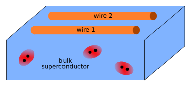
Figure 1: The physical picture for the TSC model studied in this paper: two fermionic wires are placed on top of a bulk s-wave superconductor. The wires interact with the bulk superconductor by exchanging pairs of fermions, and the total number of fermions in the wires plus the superconductor is always conserved.

We label the two wires by $\alpha\in\{1,2\}$ and we label the sites on each wire by $j\in\{1,\dots,L\}$, where $L$ is the length of each wire. The operator that annihilates a spinless fermion on site $j$ and wire $\alpha$ is $c_{j,\alpha}$, and these operators obey the standard anticommutation relations: $\{c_{j,\alpha},c_{j^{\prime},\beta}\}=0$ and $\{c_{j,\alpha},c^{\dagger}_{j^{\prime},\beta}\}=\delta_{jj^{\prime}}\delta_{\alpha\beta}$. We define the number operators $n_{j,\alpha}=c^{\dagger}_{j,\alpha}c_{j,\alpha}$ in the usual way. We also define the number operator $\mathcal{N}_{w,\alpha}$ for wire $\alpha$ as $\mathcal{N}_{w,\alpha}=\sum_{j=1}^{L}n_{j,\alpha}$. The number operator $\mathcal{N}_{w}$ for both wires together is then given by $\mathcal{N}_{w}=\sum_{\alpha=1}^{2}\mathcal{N}_{w,\alpha}$.

The number and phase degree of freedom that represents the bulk SC is comprised of the operators $\hat{n}$ and $\hat{\phi}$. We use a hat for these operators in order to distinguish the phase operator $\hat{\phi}$ from classical phases $\phi$ that appear in various parts of our analysis. The operator $\hat{n}$ is defined to have integer eigenvalues, and $\hat{n}$ and $\hat{\phi}$ obey the usual commutation relations $[\hat{\phi},\hat{n}]=i$. The Hilbert space $\mathcal{H}_{\text{SC}}$ of the number and phase degree of freedom is spanned by the states $|p\rangle$, where $p\in\mathbb{Z}$ and we have $\hat{n}|p\rangle=p|p\rangle$ and $e^{\pm i\hat{\phi}}|p\rangle=|p\pm 1\rangle$. The total Hilbert space of our model is then the tensor product $\mathcal{F}\otimes\mathcal{H}_{\text{SC}}$, where $\mathcal{F}$ is the Fock space for the fermions $c_{j,\alpha}$ on the two wires.

The operator $\hat{n}$ counts the number of Cooper pairs in the bulk SC, and $e^{i\hat{\phi}}$ adds a Cooper pair to the bulk SC (similarly, $e^{-i\hat{\phi}}$ removes a Cooper pair). Therefore, the total number operator for our entire system is

$$\mathcal{N}=\mathcal{N}_{w}+2\hat{n}\ ,$$ (1)

where $\mathcal{N}_{w}$ is the number operator for the two wires, and the factor of two is present because each Cooper pair has twice the charge of a single fermion. The model that we study in this paper conserves the total particle number of the two wires plus the bulk SC, and so our model Hamiltonian will commute with $\mathcal{N}$.

The Hamiltonian for our model takes the general form

$$H=H_{0}+V\ .$$ (2)

The first term $H_{0}$ resembles a standard mean-field Hamiltonian Kitaev (2001) for two decoupled $p$-wave wires with open boundary conditions, but with the important difference that the wires are coupled to the bulk SC in such a way that the total particle number $\mathcal{N}$ is conserved. Specifically, $H_{0}$ is given by

$$H_{0}= -\sum_{\alpha=1}^{2}\frac{t_{\alpha}}{2}\sum_{j=1}^{L-1}(c^{\dagger}_{j,\alpha}c_{j+1,\alpha}+\text{h.c.})$$

$$- \sum_{\alpha=1}^{2}\frac{\Delta_{\alpha}}{2}\sum_{j=1}^{L-1}(c_{j,\alpha}c_{j+1,\alpha}e^{i\hat{\phi}}+\text{h.c.})$$

$$- \sum_{\alpha=1}^{2}\mu_{\alpha}\sum_{j=1}^{L}\left(n_{j,\alpha}-\frac{1}{2}\right)\ .$$ (3)

The first line contains nearest-neighbor hopping terms for the fermions in both wires, with hopping energies $t_{\alpha}$ that we take to be real and positive. The second line contains nearest-neighbor pairing terms in each wire, with pairing energies $\Delta_{\alpha}$ that we assume to be real numbers. Notice that, unlike a normal mean-field Hamiltonian, the product $c_{j,\alpha}c_{j+1,\alpha}$ appears together with the phase operator $e^{i\hat{\phi}}$, and so the pairing term in $H_{0}$ commutes with the total particle number operator $\mathcal{N}$. The physical interpretation of the term $c_{j,\alpha}c_{j+1,\alpha}e^{i\hat{\phi}}$ is that two fermions leave wire $\alpha$ and enter the bulk SC as a Cooper pair. Finally, the third line in $H_{0}$ contains a chemical potential term for each wire, with chemical potentials $\mu_{\alpha}$ that are real numbers.

The second term $V$ is a charging energy term that gives an energy cost for transferring charge from the bulk SC to the wires or vice-versa. This term takes the form

$$V =\frac{1}{2}\sum_{\alpha=1}^{2}E_{c,\alpha}(\mathcal{N}_{w,\alpha}-N_{\alpha,0})^{2}$$

$$+E_{c}^{\prime}(\mathcal{N}_{w,1}-N_{1,0})(\mathcal{N}_{w,2}-N_{2,0})\ ,$$ (4)

where the parameters appearing in this expression are as follows. First, $N_{\alpha,0}$ is the electrostatically preferred number of electrons in wire $\alpha$, which is presumably equal to the number of electrons required to make wire $\alpha$ charge neutral. Next, $E_{c,\alpha}$ and $E_{c}^{\prime}$ are (inverse) capacitance coefficients that describe the electrostatic energy cost for deviating from charge neutrality. On physical grounds we have $E_{c,\alpha},E_{c}^{\prime}\geq 0$, and in order to make $V$ positive definite we also require that

$$E_{c,1}E_{c,2}\geq(E_{c}^{\prime})^{2}\ .$$ (5)

As in Ref. Lapa and Levin, 2020, we parametrize $E_{c,\alpha}$ and $E_{c}^{\prime}$ as

$$E_{c,\alpha}=\frac{\mathcal{E}_{c,\alpha}}{L}\ \ ,\ \ E_{c}^{\prime}=\frac{\mathcal{E}_{c}^{\prime}}{L}\ ,$$ (6)

where $\mathcal{E}_{c,\alpha}$ and $\mathcal{E}_{c}^{\prime}$ are rescaled charging energies that we hold fixed in the thermodynamic limit $L\to\infty$. The general form of the charging energy term $V$, and the scaling of $E_{c,\alpha}$ and $E_{c}^{\prime}$ with $L$, follow from electrostatics considerations and capture the influence of the Coulomb interaction on processes in which charge is exchanged between the wires and the bulk SC. In particular, $V$ is the physically correct form of the charging energy when the linear dimensions of the bulk SC are comparable to the length $L$ of the wires, and when the length of the wires is much larger than their thickness and their separation from the SC.

One key feature of our model is that it does not include processes in which a single fermion enters or leaves the SC; the SC can only accommodate pairs of fermions. Our model also does not include processes where a single fermion tunnels from one wire to the other.

The physical picture that motivates these properties is as follows. The reason we neglect single fermion excitations within the SC is that we assume that the energy gap to such excitations is the largest energy scale in the system, and we think of our model as a low energy effective theory describing physics below this energy scale. Likewise, the reason we neglect single fermion tunneling between the wires is that we assume that the wires are sufficiently far apart from one another that such tunneling processes are negligible.

II.2 Main stability results

We now state our main stability result for our two-wire TSC model. Our result concerns the properties of the model in a sector of fixed total particle number equal to $N$ (the “$N$-particle sector”). In other words, we work in the sector of the total Hilbert space in which $\mathcal{N}=N$ (and $N$ can be any positive integer). Each sector of fixed total particle number can be further divided into two subsectors, with each subsector containing states with a fixed eigenvalue ($\pm 1$) of $\mathcal{P}_{1}:=(-1)^{\mathcal{N}_{w,1}}$, the fermion parity operator for the first wire. Since $H$ also commutes with $\mathcal{P}_{1}$, we can separately diagonalize $H$ in each such subsector of the $N$-particle sector.

Let $|\psi^{(N)}_{\pm}\rangle$ be the ground state of $H$ in the subsector of the $N$-particle sector with $\mathcal{P}_{1}=\pm 1$, and let $E^{(N)}_{\pm}$ be the corresponding ground state energy. Our main goal is to determine the stability of a qubit built out of the two states $|\psi^{(N)}_{+}\rangle$ and $|\psi^{(N)}_{-}\rangle$.

More precisely, we wish to determine whether the qubit states $|\psi^{(N)}_{\pm}\rangle$ have the following two properties for a finite range of parameters (i.e. without fine tuning). First, $H$ should have a finite energy gap above $E^{(N)}_{\pm}$ in the subsector of the $N$-particle sector with $\mathcal{P}_{1}=\pm 1$. This prevents each qubit state from mixing (e.g., due to thermal fluctuations at low but non-zero temperatures) with other states in the same subsector of the $N$-particle sector. Second, the energy splitting $|E^{(N)}_{+}-E^{(N)}_{-}|$ between the two qubit states should be exponentially small in the system size $L$. This property is known to hold in the mean-field p-wave wire model, and it guarantees that the qubit will take a very long time to decohere.

The main result of this paper is a rigorous proof of the second property: we derive an exponential bound on the energy splitting $|E^{(N)}_{+}-E^{(N)}_{-}|$ between the two qubit states, and we show that this bound holds for a wide range of parameter values. Conveniently, the methods we use to prove this bound on the splitting also provide a proof of the first property – i.e. the existence of a finite energy gap in each of the two subsectors of the $N$-particle sector. We note that the existence of a finite energy gap can also be established by a straightforward generalization of the arguments from Ref. Lapa and Levin, 2020.

We need to define a few more parameters before we can state our main result. The first of these are a set of modified chemical potentials $\tilde{\mu}_{\alpha}$ for the two wires:

$$\tilde{\mu}_{1} =\mu_{1}+\frac{\mathcal{E}_{c,1}}{L}\left(N_{1,0}-\frac{L}{2}\right)+\frac{\mathcal{E}_{c}^{\prime}}{L}\left(N_{2,0}-\frac{L}{2}\right)$$ (7a)

$$\tilde{\mu}_{2} =\mu_{2}+\frac{\mathcal{E}_{c,2}}{L}\left(N_{2,0}-\frac{L}{2}\right)+\frac{\mathcal{E}_{c}^{\prime}}{L}\left(N_{1,0}-\frac{L}{2}\right)\ .$$ (7b)

We will see why the $\tilde{\mu}_{1}$ and $\tilde{\mu}_{2}$ parameters are natural in Sec. III when we map our Hamiltonian onto a spin model, but the basic idea is that they come from expanding the charging energy terms around half-filling.

Finally, we introduce one more parameter $\lambda$, which is defined to be the largest (in magnitude) of all the charging energies and modified chemical potentials $\tilde{\mu}_{\alpha}$:

$$\lambda =\max(|\mathcal{E}_{c,1}|,|\mathcal{E}_{c,2}|,|\mathcal{E}_{c}^{\prime}|,|\tilde{\mu}_{1}|,|\tilde{\mu}_{2}|)\ .$$ (8)

We will present our result for a particular choice of $t_{\alpha},\Delta_{\alpha}$, namely $t_{\alpha}=\Delta_{\alpha}$. The reason for this choice is as follows: for a single copy of Kitaev’s p-wave wire model, it is known that the topological superconductor phase corresponds to the region in parameter space in which $|\mu|<t$ and $\Delta\neq 0$. In particular, for any non-zero value of $\Delta$, the transition from the topological to the trivial superconducting phase always occurs at $|\mu|=t$. Since the location of the transition does not depend on the precise value of $\Delta$, we are free to pick whatever $\Delta$ is most convenient. Here we choose to study our model at the point $t_{\alpha}=\Delta_{\alpha}$ as this makes our stability analysis of the model more straightforward and transparent. If we wanted to, we could prove similar results for small deviations from the point $t_{\alpha}=\Delta_{\alpha}$ by treating the deviation as an additional short-range perturbation of the unperturbed Hamiltonian with $t_{\alpha}=\Delta_{\alpha}$.

We are now ready to state our main result.

Theorem 1.

Consider the two wire Hamiltonian $H$ at the special point $t_{\alpha}=\Delta_{\alpha}$. There exists a $L$-independent constant $\lambda_{0}>0$ such that, if $\lambda<\lambda_{0}$, then (1) $H$ has a unique ground state and a finite energy gap in each subsector of the $N$-particle sector with fixed $\mathcal{P}_{1}$ eigenvalue, and (2) the energy splitting $|E^{(N)}_{+}-E^{(N)}_{-}|$ between the ground states in the two subsectors of the $N$-particle sector satisfies the exponential bound

$$|E^{(N)}_{+}-E^{(N)}_{-}|\leq c_{1}Le^{-c_{2}L}\ ,$$ (9)

where $c_{1}$ and $c_{2}$ are fixed positive constants that depend on $\Delta_{\alpha}$, $\tilde{\mu}_{\alpha}$, $\mathcal{E}_{c,\alpha}$, and $\mathcal{E}_{c}^{\prime}$, but not on $L$.

This theorem shows that, for small enough $|\tilde{\mu}_{\alpha}|$, $|\mathcal{E}_{c,\alpha}|$, and $|\mathcal{E}_{c}^{\prime}|$, our number-conserving TSC model has both of the stability properties (i) and (ii) that we discussed above. (As a side note, it is worth pointing out that the theorem holds for any signs of the charging energy terms, though, in our setting, the model only makes physical sense when the charging energy terms are positive).

III Proof of the main result

In this section we present the proof of Theorem 1. The core of the proof is the general stability result for spin Hamiltonians with long-range interactions established in Ref. Lapa and Levin, 2023. To apply that result to our model, we first need to map our model to a suitable spin Hamiltonian. We do that in two steps. In the first step we show that, in the $N$-particle sector, our model is equivalent to a purely fermionic model without number conservation and restricted to the sector of fixed fermion parity equal to $(-1)^{N}$. In the second step, we convert this purely fermionic model to a spin model using a Jordan-Wigner transformation.

III.1 Relation to a fermionic model

We begin by mapping our full model to a purely fermionic model. Our discussion in this subsection closely follows Sec. III of the Supplemental Material from Ref. Lapa and Levin, 2020.

We start by considering the mean-field Hamiltonian $H_{\text{MF}}(\phi)$ that is obtained by replacing the operator $e^{i\hat{\phi}}$ in $H_{0}$ with the classical phase $e^{i\phi}$,

$$H_{\text{MF}}(\phi)= -\sum_{\alpha=1}^{2}\frac{t_{\alpha}}{2}\sum_{j=1}^{L-1}(c^{\dagger}_{j,\alpha}c_{j+1,\alpha}+\text{h.c.})$$

$$- \sum_{\alpha=1}^{2}\frac{\Delta_{\alpha}}{2}\sum_{j=1}^{L-1}(c_{j,\alpha}c_{j+1,\alpha}e^{i\phi}+\text{h.c.})$$

$$- \sum_{\alpha=1}^{2}\mu_{\alpha}\sum_{j=1}^{L}\left(n_{j,\alpha}-\frac{1}{2}\right)\ .$$ (10)

The Hamiltonian $H_{\text{MF}}(\phi)$ acts on only on the Fock space $\mathcal{F}$ for the fermions $c_{j,\alpha}$. The number and phase degree of freedom is not involved in $H_{\text{MF}}(\phi)$.

Let $|\chi_{a}(\phi)\rangle$, with $a\in\{0,1,2,\dots\}$, be the eigenstates of $H_{\text{MF}}(\phi)$ in the sector of the Fock space with fermion parity $(-1)^{N}$, and let $\epsilon_{a}$ be the energies of these states: $H_{\text{MF}}(\phi)|\chi_{a}(\phi)\rangle=\epsilon_{a}|\chi_{a}(\phi)\rangle$. The energies $\epsilon_{a}$ are independent of $\phi$ due to the fact that $H_{\text{MF}}(\phi)$ is related to $H_{\text{MF}}(0)$ by a unitary transformation: $H_{\text{MF}}(\phi)=e^{-i\frac{\phi}{2}\mathcal{N}_{w}}H_{\text{MF}}(0)e^{i\frac{\phi}{2}\mathcal{N}_{w}}$. This transformation also implies that the eigenstates of $H_{\text{MF}}(\phi)$ are related to the eigenstates of $H_{\text{MF}}(0)$ as $|\chi_{a}(\phi)\rangle=e^{-i\frac{\phi}{2}\mathcal{N}_{w}}|\chi_{a}(0)\rangle$.

It turns out that there is a one-to-one correspondence between the mean-field eigenstates $|\chi_{a}(\phi)\rangle$ and the eigenstates of the number-conserving Hamiltonian $H_{0}$ in a fixed $N$-particle sector. To explain this correspondence, let $|p\rangle$ be the eigenstates of the Cooper pair number operator $\hat{n}$, and let $|\phi\rangle$ be the dual set of eigenstates of $e^{i\hat{\phi}}$ that are related to $|p\rangle$ by

$$\langle\phi|p\rangle=\frac{1}{\sqrt{2\pi}}e^{ip\phi}\ .$$ (11)

In this notation, the eigenstates of $H_{0}$ in the $N$-particle sector take the form

$$|\chi^{(N)}_{a}\rangle=\frac{1}{\sqrt{2\pi}}\int_{0}^{2\pi}d\phi\ e^{i\frac{N}{2}\phi}|\chi_{a}(\phi)\rangle\otimes|\phi\rangle\ .$$ (12)

It is not hard to check that these states satisfy $H_{0}|\chi^{(N)}_{a}\rangle=\epsilon_{a}|\chi^{(N)}_{a}\rangle$ and $\mathcal{N}|\chi^{(N)}_{a}\rangle=N|\chi^{(N)}_{a}\rangle$ (see e.g. Sec. III of the Supplemental Material from Ref. Lapa and Levin, 2020 for details). In addition, these states have the following important property. Let $\mathcal{O}$ be any operator formed from the fermionic creation and annihilation operators $c_{j,\alpha}$ and $c^{\dagger}_{j,\alpha}$ that also commutes with the particle number operator for the wires, $[\mathcal{O},\mathcal{N}_{w}]=0$. Then for any two states $|\chi^{(N)}_{a}\rangle$ and $|\chi^{(N)}_{b}\rangle$, we have the identity

$$\langle\chi^{(N)}_{a}|\mathcal{O}|\chi^{(N)}_{b}\rangle=\langle\chi_{a}(0)|\mathcal{O}|\chi_{b}(0)\rangle\ .$$ (13)

To prove Eq. (13), we simply evaluate the matrix element $\langle\chi^{(N)}_{a}|\mathcal{O}|\chi^{(N)}_{b}\rangle$ using our formula Eq. (12) for $|\chi^{(N)}_{a}\rangle$, the orthogonality relation $\langle\phi|\phi^{\prime}\rangle=\delta(\phi-\phi^{\prime})$, the fact that $|\chi_{a}(\phi)\rangle=e^{-i\frac{\phi}{2}\mathcal{N}_{w}}|\chi_{a}(0)\rangle$, and our assumption that $[\mathcal{O},\mathcal{N}_{w}]=0$. We have

$$\langle\chi^{(N)}_{a}|\mathcal{O}|\chi^{(N)}_{b}\rangle = \frac{1}{2\pi}\int_{0}^{2\pi}d\phi\int_{0}^{2\pi}d\phi^{\prime}\ e^{-i\frac{N}{2}\phi}e^{i\frac{N}{2}\phi^{\prime}}\langle\chi_{a}(\phi)|\mathcal{O}|\chi_{b}(\phi^{\prime})\rangle\langle\phi|\phi^{\prime}\rangle$$ (14)

$$= \frac{1}{2\pi}\int_{0}^{2\pi}d\phi\int_{0}^{2\pi}d\phi^{\prime}\ e^{-i\frac{N}{2}\phi}e^{i\frac{N}{2}\phi^{\prime}}\langle\chi_{a}(\phi)|\mathcal{O}|\chi_{b}(\phi^{\prime})\rangle\delta(\phi-\phi^{\prime})$$

$$= \frac{1}{2\pi}\int_{0}^{2\pi}d\phi\ \langle\chi_{a}(\phi)|\mathcal{O}|\chi_{b}(\phi)\rangle$$

$$= \frac{1}{2\pi}\int_{0}^{2\pi}d\phi\ \langle\chi_{a}(0)|e^{i\frac{\phi}{2}\mathcal{N}_{w}}\mathcal{O}e^{-i\frac{\phi}{2}\mathcal{N}_{w}}|\chi_{b}(0)\rangle$$

$$= \frac{1}{2\pi}\int_{0}^{2\pi}d\phi\ \langle\chi_{a}(0)|\mathcal{O}|\chi_{b}(0)\rangle$$

$$= \langle\chi_{a}(0)|\mathcal{O}|\chi_{b}(0)\rangle\ .$$

With these results, we can now map $H$ onto a purely fermionic Hamiltonian. To do this, we consider the matrix elements of $H$ in the $|\chi^{(N)}_{a}\rangle$ basis. First, we clearly have

$$\langle\chi^{(N)}_{a}|H_{0}|\chi^{(N)}_{b}\rangle=\epsilon_{a}\delta_{ab}=\langle\chi_{a}(0)|H_{\text{MF}}(0)|\chi_{b}(0)\rangle\ ,$$ (15)

which follows directly from the construction of the states $|\chi^{(N)}_{a}\rangle$ from the states $|\chi_{a}(\phi)\rangle$. Next, for the charging energy term we also find that

$$\langle\chi^{(N)}_{a}|V|\chi^{(N)}_{b}\rangle=\langle\chi_{a}(0)|V|\chi_{b}(0)\rangle\ ,$$ (16)

which follows immediately from Eq. (13) and the fact that $V$ depends only on the number operators $\mathcal{N}_{w,\alpha}$ for the wires. Adding together (15) and (16), we conclude that the matrix elements $\langle\chi^{(N)}_{a}|H|\chi^{(N)}_{b}\rangle$ of our Hamiltonian in the $N$-particle sector are equal to the matrix elements $\langle\chi_{a}(0)|H_{\text{F}}|\chi_{b}(0)\rangle$ of a number-non-conserving fermionic Hamiltonian $H_{\text{F}}$, defined by

$$H_{\text{F}}=H_{\text{MF}}(0)+V\ ,$$ (17)

in the sector with fermion parity equal to $(-1)^{N}$.

This completes the mapping of our model (within a sector of fixed total particle number) to a purely fermionic model without number conservation (and restricted to a sector of fixed fermion parity).

III.2 Mapping to a spin model via Jordan-Wigner transformation

We now move on to the second step in the mapping to a spin Hamiltonian, which is to use a Jordan-Wigner (JW) transformation to map the fermionic Hamiltonian $H_{\text{F}}$ from Eq. (17) into a spin Hamiltonian. Since the JW transformation is a standard method, we give only a brief description of the most important points.

First, as we discussed in Sec. II, to simplify our analysis we work at the point in parameter space where $t_{\alpha}=\Delta_{\alpha}$. At this point it is helpful to first rewrite $H_{\text{F}}$ in terms of Majorana fermion operators before doing the JW transformation. For each wire $\alpha$ we define two Majorana fermion operators $a_{j,\alpha}$ and $b_{j,\alpha}$ on each site $j$ as

$$a_{j,\alpha} = -i(c_{j,\alpha}-c^{\dagger}_{j,\alpha})$$ (18a)

$$b_{j,\alpha} = c_{j,\alpha}+c^{\dagger}_{j,\alpha}\ .$$ (18b)

In terms of these operators we have the identity

$$c^{\dagger}_{j,\alpha}c_{j+1,\alpha}+c_{j,\alpha}c_{j+1,\alpha}+\text{h.c.}=ib_{j,\alpha}a_{j+1,\alpha}\ ,$$ (19)

which holds for all $j\in\{1,\dots,L-1\}$. For all $j$, we also have the identity

$$n_{j,\alpha}-\frac{1}{2}=-\frac{1}{2}ia_{j,\alpha}b_{j,\alpha}\ .$$ (20)

These two identities are sufficient to completely rewrite $H_{\text{F}}$ in terms of the Majorana operators. For example, we have (at $t_{\alpha}=\Delta_{\alpha}$)

$$H_{\text{MF}}(0)=-\sum_{\alpha=1}^{2}\frac{\Delta_{\alpha}}{2}\sum_{j=1}^{L-1}ib_{j,\alpha}a_{j+1,\alpha}+\sum_{\alpha=1}^{2}\frac{\mu_{\alpha}}{2}\sum_{j=1}^{L}ia_{j,\alpha}b_{j,\alpha}\ .$$ (21)

In addition, the number operator $\mathcal{N}_{w,\alpha}$ for wire $\alpha$ takes the form

$$\mathcal{N}_{w,\alpha}=\frac{L}{2}-\frac{1}{2}\sum_{j=1}^{L}ia_{j,\alpha}b_{j,\alpha}\ ,$$ (22)

and this identity can be used to rewrite the charging energy term in $H_{\text{F}}$ in terms of the Majorana operators.

We now turn to the JW transformation itself. For this transformation we introduce two sets of Pauli matrices $\left\{\sigma^{x}_{j,\alpha},\sigma^{y}_{j,\alpha},\sigma^{z}_{j,\alpha}\right\}$ (one set for each wire). For the fermions on the first wire the transformation between the Majorana operators and the Pauli matrices $\sigma^{x,y,z}_{j,\alpha}$ is

$$a_{j,1} = \left(\prod_{k<j}\sigma^{x}_{k,1}\right)\sigma^{z}_{j,1}$$ (23a)

$$b_{j,1} = \left(\prod_{k<j}\sigma^{x}_{k,1}\right)\sigma^{y}_{j,1}\ .$$ (23b)

For the second wire the relation is slightly more complicated because we have to ensure that Majorana operators on two different wires still anticommute with each other. Therefore, for the fermions on the second wire we have the transformation

$$a_{j,2} = \left(\prod_{\ell=1}^{L}\sigma^{x}_{\ell,1}\right)\left(\prod_{k<j}\sigma^{x}_{k,2}\right)\sigma^{z}_{j,2}$$ (24)

$$b_{j,2} = \left(\prod_{\ell=1}^{L}\sigma^{x}_{\ell,1}\right)\left(\prod_{k<j}\sigma^{x}_{k,2}\right)\sigma^{y}_{j,2}\ .$$ (25)

To rewrite the fermionic Hamiltonian $H_{\text{F}}$ in terms of the spin operators, it will also be convenient to introduce the following notation for sums of $\sigma^{x}_{j,\alpha}$ operators: $\Sigma^{x}_{\alpha}=\sum_{j=1}^{L}\sigma^{x}_{j,\alpha}$.

After the JW transformation, the mean-field part of the Hamiltonian takes the form

$$H_{\text{MF}}(0)=-\sum_{\alpha=1}^{2}\frac{\Delta_{\alpha}}{2}\sum_{j=1}^{L-1}\sigma^{z}_{j,\alpha}\sigma^{z}_{j+1,\alpha}+\sum_{\alpha=1}^{2}\frac{\mu_{\alpha}}{2}\Sigma^{x}_{\alpha}\ ,$$ (26)

and the charging energy term is now

$$V =\frac{1}{2}\sum_{\alpha=1}^{2}\frac{\mathcal{E}_{c,\alpha}}{L}\left(\frac{1}{2}\Sigma^{x}_{\alpha}+N_{\alpha,0}-\frac{L}{2}\right)^{2}$$

$$+\frac{\mathcal{E}_{c}^{\prime}}{L}\left(\frac{1}{2}\Sigma^{x}_{1}+N_{1,0}-\frac{L}{2}\right)\left(\frac{1}{2}\Sigma^{x}_{2}+N_{2,0}-\frac{L}{2}\right)\ .$$ (27)

The entire Hamiltonian $H_{\text{F}}$ can then be rewritten as

$$H_{\text{F}} =\sum_{\alpha=1}^{2}\frac{\Delta_{\alpha}}{2}\sum_{j=1}^{L-1}\left(1-\sigma^{z}_{j,\alpha}\sigma^{z}_{j+1,\alpha}\right)+\sum_{\alpha=1}^{2}\frac{\tilde{\mu}_{\alpha}}{2}\Sigma^{x}_{\alpha}$$

$$+\sum_{\alpha=1}^{2}\frac{\mathcal{E}_{c,\alpha}}{8L}\sum_{j,j^{\prime}=1}^{L}\sigma^{x}_{j,\alpha}\sigma^{x}_{j^{\prime},\alpha}(1-\delta_{j,j^{\prime}})$$

$$+\frac{\mathcal{E}_{c}^{\prime}}{4L}\Sigma^{x}_{1}\Sigma^{x}_{2}+\text{constant}\ ,$$ (28)

where the $\tilde{\mu}_{\alpha}$ are the modified chemical potentials that we defined in Eqs. (7). In particular, the form of the JW-transformed Hamiltonian explains why it is $\tilde{\mu}_{\alpha}$, and not $\mu_{\alpha}$, that appears in our main result.

Finally, we need to discuss the various fermion parity operators and their form in terms of spin operators. First, the total fermion parity operator $(-1)^{\mathcal{N}_{w}}$ takes the form

$$(-1)^{\mathcal{N}_{w}}=\mathcal{S}\ ,$$ (29)

where $\mathcal{S}$ is the total Ising symmetry operator for both wires: $\mathcal{S}=\prod_{\alpha=1}^{2}\prod_{j=1}^{L}\sigma^{x}_{j,\alpha}$. Next, we consider the fermion parity operators for each individual wire. Using the JW transformation, we find that $\mathcal{N}_{w,\alpha}=\frac{L}{2}-\frac{1}{2}\Sigma^{x}_{\alpha}$, and so

$$\mathcal{P}_{\alpha}:=(-1)^{\mathcal{N}_{w,\alpha}}=\mathcal{S}_{\alpha}\ ,$$ (30)

where $\mathcal{S}_{\alpha}=\prod_{j=1}^{L}\sigma^{x}_{j,\alpha}$ is the Ising symmetry operator for wire $\alpha$.

If we put all of our results together, then we find that studying our original model in the subsector of the $N$-particle sector where $\mathcal{P}_{1}=\pm 1$ is equivalent to studying the Hamiltonian $H_{\text{F}}$ (expressed in terms of spin operators) in the $\mathcal{S}_{1}=\pm 1$ subsector of the sector with $\mathcal{S}=(-1)^{N}$.

III.3 Completing the proof

At this point we have mapped our model to a spin Hamiltonian with long-range $\sigma^{x}_{j,\alpha}\sigma^{x}_{j^{\prime},\beta}$ interactions. We now show that this spin Hamiltonian is subject to the general stability result that we proved in Ref. Lapa and Levin, 2023.

To apply our result from Ref. Lapa and Levin, 2023, notice that the final spin Hamiltonian from Eq. (28) (after dropping the constant part) can be written in the general form

$$H_{\text{spin}}=\sum_{\alpha=1}^{2}\frac{\Delta_{\alpha}}{2}\sum_{j=1}^{L-1}\left(1-\sigma^{z}_{j,\alpha}\sigma^{z}_{j+1,\alpha}\right)+\lambda W\ ,$$ (31)

where $\lambda$ is a constant with units of energy and the perturbation term $W$ takes the form

$$W=\sum_{\alpha=1}^{2}h_{\alpha}\Sigma^{x}_{\alpha}+\frac{1}{2}\sum_{j,j^{\prime}=1}^{L}\sum_{\alpha,\beta=1}^{2}f^{(\alpha,\beta)}(|j-j^{\prime}|)\sigma^{x}_{j,\alpha}\sigma^{x}_{j^{\prime},\beta}\ .$$ (32)

Here, $h_{\alpha}$ and $f^{(\alpha,\beta)}(|j-j^{\prime}|)$ are dimensionless coefficients, and we assume that $f^{(\alpha,\beta)}(0)=0$ if $\alpha=\beta$ to avoid including constant terms in $W$. In particular, we can choose the following values for $\lambda$, $h_{\alpha}$, and $f^{(\alpha,\beta)}(|j-j^{\prime}|)$:

$$\lambda=\max(|\mathcal{E}_{c,1}|, |\mathcal{E}_{c,2}|,|\mathcal{E}_{c}^{\prime}|,|\tilde{\mu}_{1}|,|\tilde{\mu}_{2}|)$$ (33a)

$$h_{\alpha} =\frac{\tilde{\mu}_{\alpha}}{2\lambda}$$ (33b)

$$f^{(1,1)}(|j-j^{\prime}|) =\frac{\mathcal{E}_{c,1}}{4\lambda L}(1-\delta_{j,j^{\prime}})$$ (33c)

$$f^{(2,2)}(|j-j^{\prime}|) =\frac{\mathcal{E}_{c,2}}{4\lambda L}(1-\delta_{j,j^{\prime}})$$ (33d)

$$f^{(1,2)}(|j-j^{\prime}|) =\frac{\mathcal{E}_{c}^{\prime}}{4\lambda L}$$ (33e)

$$f^{(2,1)}(|j-j^{\prime}|) =f^{(1,2)}(|j-j^{\prime}|)\ .$$ (33f)

Notice that the coefficients $f^{(\alpha,\beta)}(|j-j^{\prime}|)$ are bounded in magnitude by $\frac{1}{4L}$ and therefore, in particular,

$$|f^{(\alpha,\beta)}(|j-j^{\prime}|)|\leq 1\ .$$ (34)

Also, for any site $j$ the coefficients $f^{(\alpha,\beta)}(|j-j^{\prime}|)$ satisfy a summability condition of the form

$$\sum_{j^{\prime},\alpha,\beta}\left|f^{(\alpha,\beta)}(|j-j^{\prime}|)\right|\leq c\ ,$$ (35)

where $c$ is a constant that can be chosen to be independent of $L$. (Specifically, in this case, we can take $c=1$).

With this setup, we are now in a position to apply the stability result from Ref. Lapa and Levin, 2023 (adapted to the current setting).

Theorem (Adapted from Theorem 1 of Ref. Lapa and Levin, 2023).

Consider a Hamiltonian $H_{\text{spin}}$ of the form (31) with interaction coefficients that satisfy (34) and (35). There exists a $L$-independent constant $\lambda_{0}>0$ such that, if $|\lambda|<\lambda_{0}$, then (1) $H_{\text{spin}}$ has a unique ground state and a finite energy gap in each subsector of the $\mathcal{S}=(-1)^{N}$ sector with fixed $\mathcal{S}_{1}$ eigenvalue, and (2) the ground state energy splitting $|E_{+}(\lambda)-E_{-}(\lambda)|$ between the $\mathcal{S}_{1}=\pm 1$ subsectors of the $\mathcal{S}=(-1)^{N}$ sector satisfies the exponential bound

$$|E_{+}(\lambda)-E_{-}(\lambda)|\leq c_{1}Le^{-c_{2}L}\ ,$$ (36)

where $c_{1}$ and $c_{2}$ are positive constants that depend on $\Delta_{\alpha}$, $h_{\alpha}$, and $\lambda$, but not on $L$.

Combining the above theorem with the mappings discussed in the previous sections, Theorem 1 follows immediately.

A final comment: as we mentioned earlier, the above theorem is similar, but not identical, to Theorem 1 of Ref. Lapa and Levin, 2023. The main difference is that the original theorem was phrased in terms of a single spin chain, while the above theorem involves two coupled spin chains. Also, while the original theorem assumed periodic boundary conditions, here we consider a model with open boundary conditions. These minor modifications in the statement of the theorem can be accommodated by making minor technical changes to the proofs in Ref. Lapa and Levin, 2023. For completeness we summarize these changes in Appendix A.

IV Conclusion

In this paper we have completed the work that we began in Ref. Lapa and Levin, 2020: combining the results of this paper and Ref. Lapa and Levin, 2020, we have now proved that three of the key properties of the mean-field TSC models also hold in a number-conserving toy model of a qubit formed from a 1D TSC. These properties are: (i) the existence of two low-energy “qubit” states that are separated from the rest of the spectrum by a finite energy gap; (ii) an exponentially small bound on the energy splitting of the qubit states (the main contribution of this paper); and (iii) the existence of long-range “Majorana-like” correlations between the ends of the fermionic wires in the 1D TSC model. These results provide an important proof of principle that the key properties of the mean-field TSC models — properties that are important for quantum computing applications — can indeed be realized in a number-conserving model without fine-tuning.

A natural next step would be to study the above properties in a more realistic model. Such a model would include some or all of the following ingredients: first, the bulk s-wave SC would be modeled by a 3D number-conserving Hamiltonian of interacting fermions (rather than a single number and phase degree of freedom). Second, the 1D wires would couple to the 3D bulk via single-particle hopping terms (rather than pair hopping terms). Finally, the fermions would interact via microscopic Coulomb interactions (rather than an effective charging energy term). While it is not obvious how to generalize our techniques to this setting, we see this as an interesting direction for future work.

Appendix A Applying our stability results to the two-wire model in this paper

As we mentioned in the main text, we need to make a few changes to our setup and proofs from Ref. Lapa and Levin, 2023 in order to apply the stability results from that paper to the spin model from Eq. (28). There are two main differences between this spin model and the model that we studied in Ref. Lapa and Levin, 2023 (see Eqs. (2.1)-(2.3) of that paper). The first difference is that the unperturbed spin model in this paper consists of two transverse-field Ising chains, instead of one, and the long-range interaction term (which comes from the charging energy term) couples spins within and between the two chains. The second difference is that the model in this paper has open boundary conditions for the two chains, while we assumed periodic boundary conditions in Ref. Lapa and Levin, 2023.

We now give a brief list of the main changes that we need to make in the setup and proofs of Ref. Lapa and Levin, 2023 in order to apply the results of that paper to Eq. (28) of this paper. In what follows we assume that any reader of this appendix is familiar with the concepts and notation from Ref. Lapa and Levin, 2023.

Changes needed because of the open boundary conditions:

• Sums over the separation $r=|j-j^{\prime}|$ between sites $j$ and $j^{\prime}$ on the spin chains now run from $1$ to $L-1$ instead of $1$ to $L/2$.

• The size of the blocked spacetime lattice $\Lambda$ used in the polymer expansion is now $|\Lambda|=(2L-1)M$ instead of $2LM$. Compared to the periodic case, the lattice is now missing one column of plaquettes.

• Support sets can now include “half-boxes” at the boundaries of the system. These do not introduce any complications and they can be treated exactly the same as the full boxes in the bulk of the system.

Changes needed because we now have two wires (two spin chains):

• The weights $W_{\pm}(X)$ are now for the system restricted to the $\mathcal{S}_{1}=\pm 1$ subsectors of the $\mathcal{S}=(-1)^{N}$ sector of the Hilbert space for the two spin chains.

• We now define the macroscopic support set $s(\mathcal{C})$ of a microscopic domain wall and interaction configuration $\mathcal{C}$ as follows.

  1. If $\mathcal{C}$ has a domain wall worldline (from either wire) that passes all the way through a given plaquette, then that plaquette is included in $s(\mathcal{C})$.

  2. If a perturbation term $V_{Y}$ has support on site $j$ (on either wire) within the time interval $[\tau(\ell-1),\tau\ell]$, then $s(\mathcal{C})$ contains the box or half-box centered on $j$ within that time slice.

  3. If a perturbation term $V_{Y}$ has support on site $j$ (on either wire) and site $k$ (on either wire) within the time interval $[\tau(\ell-1),\tau\ell]$, then $s(\mathcal{C})$ contains a single dashed line connecting the boxes or half-boxes centered on sites $j$ and $k$ within that time slice. Of course, this rule is only relevant for the $\sigma^{x}\sigma^{x}$ terms.

• With the new definition of $s(\mathcal{C})$ from the previous bullet point, there are now more microscopic configurations that lead to the same macroscopic support set, and we need to be sure to sum over these additional configurations when deriving the bound on the weights $W_{\pm}(X)$ from Lemma 1 of Ref. Lapa and Levin, 2023. In particular, this means that the “partial perturbation terms” $\mathcal{V}_{\ell}$ from Eq. (A17) of Ref. Lapa and Levin, 2023 now contain more terms, and the constant $K$ that first appears in Eq. (A23) will be larger.

• The parameter $\Delta$ that appears in the upper bound in Eq. (A4) of Ref. Lapa and Levin, 2023 should be chosen as $\Delta=\min(\Delta_{1},\Delta_{2})$. The reason is that this upper bound is now obtained by taking the smaller of the two excitation energies for domain walls in the unperturbed Hamiltonian.

• The parameter $|h|$ in Eq. (A7) of Ref. Lapa and Levin, 2023 should be chosen as $|h|=\max(|h_{1}|,|h_{2}|)$.

• In Eq. (A7) of Ref. Lapa and Levin, 2023, the weights in the “$+$” and “$-$” Ising sectors are both bounded from above by an expression that features a trace over only the “$+$” Ising sector. Instead of this, we now have a bound in which the weights in the $\mathcal{S}=(-1)^{N}$, $\mathcal{S}_{1}=\pm 1$ subsectors are both bounded from above by an expression that features a trace in the $\mathcal{S}=1$, $\mathcal{S}_{1}=1$ subsector.

References

- Kitaev (2001) A. Y. Kitaev, Physics-Uspekhi 44, 131 (2001).
- Read and Green (2000) N. Read and D. Green, Phys. Rev. B 61, 10267 (2000).
- Lutchyn et al. (2010) R. M. Lutchyn, J. D. Sau, and S. Das Sarma, Phys. Rev. Lett. 105, 077001 (2010).
- Oreg et al. (2010) Y. Oreg, G. Refael, and F. von Oppen, Phys. Rev. Lett. 105, 177002 (2010).
- Nadj-Perge et al. (2013) S. Nadj-Perge, I. K. Drozdov, B. A. Bernevig, and A. Yazdani, Phys. Rev. B 88, 020407(R) (2013).
- Mourik et al. (2012) V. Mourik, K. Zuo, S. M. Frolov, S. R. Plissard, E. P. A. M. Bakkers, and L. P. Kouwenhoven, Science 336, 1003 (2012).
- Das et al. (2012) A. Das, Y. Ronen, Y. Most, Y. Oreg, M. Heiblum, and H. Shtrikman, Nature Physics 8, 887 (2012).
- Rokhinson et al. (2012) L. P. Rokhinson, X. Liu, and J. K. Furdyna, Nat. Phys. 8, 795 (2012).
- Deng et al. (2012) M. T. Deng, C. L. Yu, G. Y. Huang, M. Larsson, P. Caroff, and H. Q. Xu, Nano Lett. 12, 6414 (2012).
- Finck et al. (2013) A. D. K. Finck, D. J. Van Harlingen, P. K. Mohseni, K. Jung, and X. Li, Phys. Rev. Lett. 110, 126406 (2013).
- Churchill et al. (2013) H. O. H. Churchill, V. Fatemi, K. Grove-Rasmussen, M. T. Deng, P. Caroff, H. Q. Xu, and C. M. Marcus, Phys. Rev. B 87, 241401(R) (2013).
- Nadj-Perge et al. (2014) S. Nadj-Perge, I. K. Drozdov, J. Li, H. Chen, S. Jeon, J. Seo, A. H. MacDonald, B. A. Bernevig, and A. Yazdani, Science 346, 602 (2014).
- Albrecht et al. (2016) S. M. Albrecht, A. Higginbotham, M. Madsen, F. Kuemmeth, T. S. Jespersen, J. Nygård, P. Krogstrup, and C. Marcus, Nature 531, 206 (2016).
- Aasen et al. (2016) D. Aasen, M. Hell, R. V. Mishmash, A. Higginbotham, J. Danon, M. Leijnse, T. S. Jespersen, J. A. Folk, C. M. Marcus, K. Flensberg, and J. Alicea, Phys. Rev. X 6, 031016 (2016).
- Chen et al. (2019) J. Chen, B. D. Woods, P. Yu, M. Hocevar, D. Car, S. R. Plissard, E. P. A. M. Bakkers, T. D. Stanescu, and S. M. Frolov, Phys. Rev. Lett. 123, 107703 (2019).
- Woods et al. (2019) B. D. Woods, J. Chen, S. M. Frolov, and T. D. Stanescu, Phys. Rev. B 100, 125407 (2019).
- Ji and Wen (2018) W. Ji and X.-G. Wen, Phys. Rev. Lett. 120, 107002 (2018).
- Huang et al. (2018) Y. Huang, F. Setiawan, and J. D. Sau, Phys. Rev. B 97, 100501(R) (2018).
- Kayyalha et al. (2020) M. Kayyalha, D. Xiao, R. Zhang, J. Shin, J. Jiang, F. Wang, Y.-F. Zhao, R. Xiao, L. Zhang, K. M. Fijalkowski, P. Mandal, M. Winnerlein, C. Gould, Q. Li, L. W. Molenkamp, M. H. W. Chan, N. Samarth, and C.-Z. Chang, Science 367, 64 (2020).
- Yu et al. (2021) P. Yu, J. Chen, M. Gomanko, G. Badawy, E. P. A. M. Bakkers, K. Zuo, V. Mourik, and S. M. Frolov, Nature Physics 17, 482 (2021).
- Frolov (2021) S. Frolov, Nature 592, 350 (2021).
- Lin and Leggett (2022) Y. Lin and A. J. Leggett, Quantum Frontiers 1, 1 (2022).
- Leggett (2015) A. J. Leggett, “http://people.physics.illinois.edu/Leggett/MZM.pdf” (2015).
- Leggett (2016) A. J. Leggett, “https://www.youtube.com/playlist?list=PLBRgytHojT9YMGLNaVjowfn829AZY1kGQ” (2016).
- Ortiz and Cobanera (2016) G. Ortiz and E. Cobanera, Ann. Phys. 372, 357 (2016).
- Lin and Leggett (2017) Y. Lin and A. J. Leggett, arXiv:1708.02578 (2017).
- Lin and Leggett (2018) Y. Lin and A. J. Leggett, arXiv:1803.08003 (2018).
- Lapa and Levin (2020) M. F. Lapa and M. Levin, Phys. Rev. Lett. 124, 257002 (2020).
- Hastings (2007) M. B. Hastings, J. Stat. Mech.: Theory Exp. 2007, P05010 (2007).
- Pfeuty (1970) P. Pfeuty, Ann. Phys. (N. Y.) 57, 79 (1970).
- Semenoff and Sodano (2007) G. W. Semenoff and P. Sodano, J. Phys. B 40, 1479 (2007).
- Semenoff and Sodano (2006) G. W. Semenoff and P. Sodano, Electron. J. Theor. Phys. 3, 157 (2006).
- Fu (2010) L. Fu, Phys. Rev. Lett. 104, 056402 (2010).
- Vijay and Fu (2016) S. Vijay and L. Fu, Phys. Rev. B 94, 235446 (2016).
- Reslen (2018) J. Reslen, J. Phys. Commun. 2, 105006 (2018).
- Lapa and Levin (2023) M. F. Lapa and M. Levin, J. Stat. Mech. 2023, 013102 (2023).
- Ortiz et al. (2014) G. Ortiz, J. Dukelsky, E. Cobanera, C. Esebbag, and C. Beenakker, Phys. Rev. Lett. 113, 267002 (2014).
- Cheng and Tu (2011) M. Cheng and H.-H. Tu, Phys. Rev. B 84, 094503 (2011).
- Fidkowski et al. (2011) L. Fidkowski, R. M. Lutchyn, C. Nayak, and M. P. A. Fisher, Phys. Rev. B 84, 195436 (2011).
- Sau et al. (2011) J. D. Sau, B. I. Halperin, K. Flensberg, and S. Das Sarma, Phys. Rev. B 84, 144509 (2011).
- Tsvelik (2011) A. Tsvelik, arXiv:1106.2996 (2011).
- Cheng and Lutchyn (2015) M. Cheng and R. Lutchyn, Phys. Rev. B 92, 134516 (2015).
- Kane et al. (2017) C. L. Kane, A. Stern, and B. I. Halperin, Phys. Rev. X 7, 031009 (2017).
- Knapp et al. (2019) C. Knapp, J. I. Väyrynen, and R. M. Lutchyn, arXiv:1909.10521 (2019).
- Ruhman et al. (2015) J. Ruhman, E. Berg, and E. Altman, Phys. Rev. Lett. 114, 100401 (2015).
- Rombouts et al. (2010) S. M. A. Rombouts, J. Dukelsky, and G. Ortiz, Phys. Rev. B 82, 224510 (2010).
- Iemini et al. (2015) F. Iemini, L. Mazza, D. Rossini, R. Fazio, and S. Diehl, Phys. Rev. Lett. 115, 156402 (2015).
- Lang and Büchler (2015) N. Lang and H. P. Büchler, Phys. Rev. B 92, 041118(R) (2015).
- Wang et al. (2017) Z. Wang, Y. Xu, H. Pu, and K. R. A. Hazzard, Phys. Rev. B 96, 115110 (2017).
- Kraus et al. (2013) C. V. Kraus, M. Dalmonte, M. A. Baranov, A. M. Läuchli, and P. Zoller, Phys. Rev. Lett. 111, 173004 (2013).
- Chen et al. (2018) C. Chen, W. Yan, C. S. Ting, Y. Chen, and F. J. Burnell, Phys. Rev. B 98, 161106(R) (2018).
- Ruhman and Altman (2017) J. Ruhman and E. Altman, Phys. Rev. B 96, 085133 (2017).
- Yin et al. (2019) X. Yin, T.-L. Ho, and X. Cui, New J. Phys. 21, 013004 (2019).
- Lapa (2020) M. F. Lapa, Phys. Rev. Res. 2, 033309 (2020).