The disordered Dicke model

Abstract

We introduce and study the disordered Dicke model in which the spin-boson couplings are drawn from a random distribution with some finite width. Regarding the quantum phase transition we show that when the standard deviation $\sigma$ of the coupling strength gradually increases, the critical value of the mean coupling strength $\mu$ gradually decreases and after a certain $\sigma$ there is no quantum phase transition at all; the system always lies in the super-radiant phase. We derive an approximate expression for the quantum phase transition in the presence of disorder in terms of $\mu$ and $\sigma$, which we numerically verify. Studying the thermal phase transition in the disordered Dicke model, we obtain an analytical expression for the critical temperature in terms of the mean and standard deviation of the coupling strength. We observe that even when the mean of the coupling strength is zero, there is a finite temperature transition if the standard deviation of the coupling is sufficiently high. Disordered couplings in the Dicke model will exist in quantum dot superlattices, and we also sketch how they can be engineered and controlled with ultracold atoms or molecules in a cavity.

I Introduction

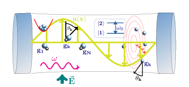
Figure 1: Schematic of the disordered Dicke model where $N$ two levels atoms are coupled to a single mode bosonic field with different spin-boson coupling strengths $g_{k}$, and two possible realisations. The frequency of the bosonic mode is $\omega$ and the gap between two levels $|1\rangle$ and $|2\rangle$ of each atom is $\omega_{0}$. (left) These could be ultra-cold molecules whose fixed transition dipoles are randomly oriented wrt. the cavity field direction (green), or (right) atoms under the influence of an additional external field that breaks their symmetry, such as the magnetic field around a wire (red).

The Dicke model [1], which describes the interaction between light and matter, is of fundamental importance within the field of quantum optics. It exhibits a variety of interesting phase transitions covering quantum phase transitions [2, 3, 4, 5, 6] (QPT), excited-state quantum phase transitions [7, 8] (ESQPT) and thermal phase transitions [9, 7, 10, 11, 8] (TPT). The QPT takes place in the thermodynamic limit of infinite atom number, $N\to\infty$, where the system goes from the normal phase (NP) to the super-radiant phase (SP) [12] at some critical coupling strength $g_{c}$ [3] between spins and bosons. If temperature is introduced to the system, for $g>g_{c}$, there is a critical temperature $T_{c}$, above which the system returns to the NP from the SP, whereas for $g<g_{c}$ the system lies in the NP for all temperatures [13, 9, 14, 15, 16, 7, 8].

Here, we generalize the standard Dicke model towards disorder in the coupling strength $g$, for which we propose several practical realisations. While the role of disorder in the more general spin-boson model has been considered both in theoretical [17, 18, 19, 20, 21, 22] and experimental [23, 24, 25] studies, the exploration of disorder-induced phenomena within this context is still at a nascent stage. We focus on those here, with the aid of tools from quantum information theory such as mutual information [26, 27, 28] between two spins as a function of temperature, whose usefulness has been demonstrated for clean Dicke models earlier [8, 29].

In the usual clean Dicke model, it is well known that the QPT [2, 3, 4, 5, 6] occurs at some critical light matter coupling strength. We find that for the disordered Dicke model both the mean and the standard deviation of the random coupling distribution play a crucial role in the QPT. If either one of them or both are high, then the ground state exhibits super-radiant behaviour. To show this, we numerically calculate the ground state energy and average boson number as a function of the coupling distribution for the disordered Dicke model. We verify our numerics with the aid of available analytical results [3] for the ground state energy and the average boson number across the QPT in the usual Dicke model. By carrying out a disorder-averaging of their results, we obtain an approximate expression for the critical line of the QPT in the disordered model. The behaviour of the observables (ground state energy and average boson number) around the critical line that we obtained using a Taylor series expansion shows broad agreement with our numerics. Moreover, we show how a symmetry of the Hamiltonian can be exploited along with a heuristic argument to obtain the line of quantum criticality in a more accurate manner.

To understand the thermal phase transition, we follow methods for which the basis was laid in Ref. [9, 30], and calculate the partition function of the disordered Dicke model to obtain the critical temperature in terms of the disorder coupling strength. Numerically we calculate the mutual information between two spins for the disordered Dicke model by a method similar to our earlier work [8] for the usual Dicke model. When the width of the disorder is sufficiently high, there is a finite temperature transition from the SP to the NP even if the mean of the coupling strength is zero. We can predict the critical temperature of this transition analytically, signatures for which are also seen in the mutual information found numerically.

Earlier studies of disorder in the Dicke model considered the multi-mode case [31]. In contrast, we sketch several possible realisations of disorder in the single mode Dicke model. It can naturally arise in semiconductor quantum dot lattices (see for e.g. [32]), where each quantum dot can have a varied orientation relative to propagating electric fields, yet due to the small structure all dots effectively radiate into a single mode, causing superradiance. One can also engineer controlled realisations, by transforming a random spatial distribution of atoms within an optical cavity [33] relative to a varying electric field amplitude into a distribution of couplings. Other possibilities include ultra-cold molecules whose fixed transition dipoles are randomly oriented with respect to the cavity field direction.

The organization of the article is as follows. In the next section we will discuss the system Hamiltonian for the disordered Dicke model. In section III and IV we present our results regarding the two types of phase transitions: QPT and TPT. In section V we outline several possible experimental realisations. Finally in section VI we provide a summary of our work.

II Model Hamiltonian and quantifiers

In Fig. 1 we show a schematic of the disordered Dicke model. The Hamiltonian consists of a single-mode bosonic field coupled to $N$ atoms with a coupling strength that is modeled as a random variable. The Hamiltonian can be written as

$$H=\omega a^{\dagger}a+\frac{\omega_{0}}{2}\sum_{i=1}^{N}\sigma_{z}^{(i)}+\frac{1}{\sqrt{N}}(a^{\dagger}+a)\sum_{i=1}^{N}g_{i}\sigma_{x}^{(i)},$$ (1)

where the operators $a$ and $a^{\dagger}$ are the bosonic annihilation and creation operators respectively, following the commutation relation $[a,a^{\dagger}]=1$ and $J_{x,z}=\sum_{i=1}^{N}\frac{1}{2}\sigma_{x,z}^{(i)}$ are the angular momentum operators of a pseudospin with length $j$, composed of $N=2j$ spin-$\frac{1}{2}$ atoms described by Pauli matrices $\sigma_{x,z}^{(i)}$ acting on site $i$. Here, the $g_{i}$’s are random numbers drawn from two types of distributions. In the first distribution, the $g_{i}$’s are drawn from a uniform unit box distribution with finite width ($2\epsilon$) and height $A$ such that $2\epsilon A=1$. The parameters $\epsilon$ and $A$ are chosen so that $2\epsilon=(\mu+\epsilon)-(\mu-\epsilon)$, $\epsilon=\sqrt{3}\sigma$ and hence $A=\frac{1}{2\sqrt{3}\sigma}$ where $\mu$ and $\sigma$ are the mean and the standard deviation. In the second distribution, we consider $g_{i}\propto\cos\theta_{i}$, where $\theta_{i}$ are angles randomly drawn from a Gaussian distribution $p(\theta)\sim\exp([-(\theta-\theta_{0})^{2}/\sigma_{\theta}^{2}])$. Both can be engineered e.g. in optical cavities as sketched in Fig. 1 and discussed in section V. Due to the disorder in the coupling strengths, $J^{2}$ is not a conserved quantity of the Hamiltonian 1 and hence we have to consider all possible spin configurations. For $N$ spins, the corresponding dimension of the spin sub-space is $2^{N}$ and the bosonic sub-space dimension is $n_{\text{max}}+1$, where $n_{\text{max}}$ is the maximal occupation we allow for the bosonic field. Hence the total Hilbert space dimension for our numerical calculations is $N_{D}=2^{N}(n_{\text{max}}+1)$.

In the next sections we explore the QPT and TPT separately, based on the properties of eigenvalues and eigenstates of Eq. (1). We study useful quantifiers such as ground state energy, average boson number and mutual information between two spins. For a mixed state (like a temperature equilibriated state), the mutual information has been shown [8] to be an appropriate quantity, although it contains both quantum and classical correlations. We shall use the mutual information [26, 27, 28, 34, 8] between two spins from a mixed density matrix. Defining the reduced density matrices of any two selected spins to be $\rho_{1}$ and $\rho_{2}$ and the reduced density matrix corresponding to the two-spin state to be $\rho_{12}$, the mutual information between the two spins can be computed using the relation:

$$I_{12}=S_{1}+S_{2}-S_{12},$$ (2)

where $S_{1,2}=-Tr(\rho_{1,2}\ln(\rho_{1,2}))$, $S_{12}=-Tr(\rho_{12}\ln(\rho_{12}))$ are the corresponding von Neumann entropies. Since we will be interested in $I_{12}$ at finite temperature, we will first construct the total thermal density matrix: $\rho_{\text{Th}}=e^{-\frac{\mathcal{H}}{k_{B}T}}$, and then trace over the bosonic subspace and the remaining $(N-2)$ or $(N-1)$ spins. Since we will average over the disorder, it does not matter which two spins are considered for the purpose of computing mutual information. Another useful observable that we use to study the QPT is the average boson number $\langle a^{\dagger}a\rangle$ evaluated in the interacting ground state.

III Quantum phase transition

It is well known that in the thermodynamic limit (when the atom number $N\to\infty$), the usual Dicke model exhibits a quantum phase transition [4] from the normal phase to the super-radiant phase at some critical coupling strength $g_{c}$. In the disordered Dicke model, if we fix the mean of the coupling strength at a sufficiently low value and vary the standard deviation ($\sigma$) we see a similar QPT. The QPT here is studied with the aid of the disorder-averged energy and average boson number in the ground state. In Figs. 2 and 4 we show these properties in the ground-state of the disordered Dicke model, considering two types of distributions as discussed in the previous section.

What we will empirically show now, is that much of the behavior of the disordered Dicke model can be understood by averaging known results for the disorder-free (clean) model. This is not clear a-priori, since all the two-level systems in the disordered model couple to the same bosonic mode, and thus get coupled. For the clean Dicke model, Emary et al [2] have derived analytical results for the ground state energy:

$$E_{G} =\begin{cases}-\frac{N\omega_{0}}{2},&g<g_{c}\\ -\frac{N\omega_{0}}{4}\left[\frac{g^{2}}{g_{c}^{2}}+\frac{g_{c}^{2}}{g^{2}}\right],&g>g_{c}\end{cases}$$ (3)

and the average boson number in the cavity:

$$\langle a^{\dagger}a\rangle =\begin{cases}0,&g<g_{c}\\ \frac{N}{\omega^{2}}\left[g^{2}-\frac{g_{c}^{4}}{g^{2}}\right]&g>g_{c}\end{cases}$$ (4)

where $g_{c}$ is the critical value of the coupling in the absence of disorder. We will make use of the above results and integrate over the coupling strength distribution to obtain approximate analytical results for the disordered Dicke model. We denote the disorder-averaged value of an observable $O$ as $\overline{O}$:

$$\overline{O}=\int_{x_{1}}^{x_{2}}P(g)O(g)dg,$$ (5)

where $P(g)$ is the distribution of the disorder and the limits of integration $x_{1}$ and $x_{2}$ have to be chosen appropriately according to the observable and the distribution being considered.

III.1 Uniform distribution

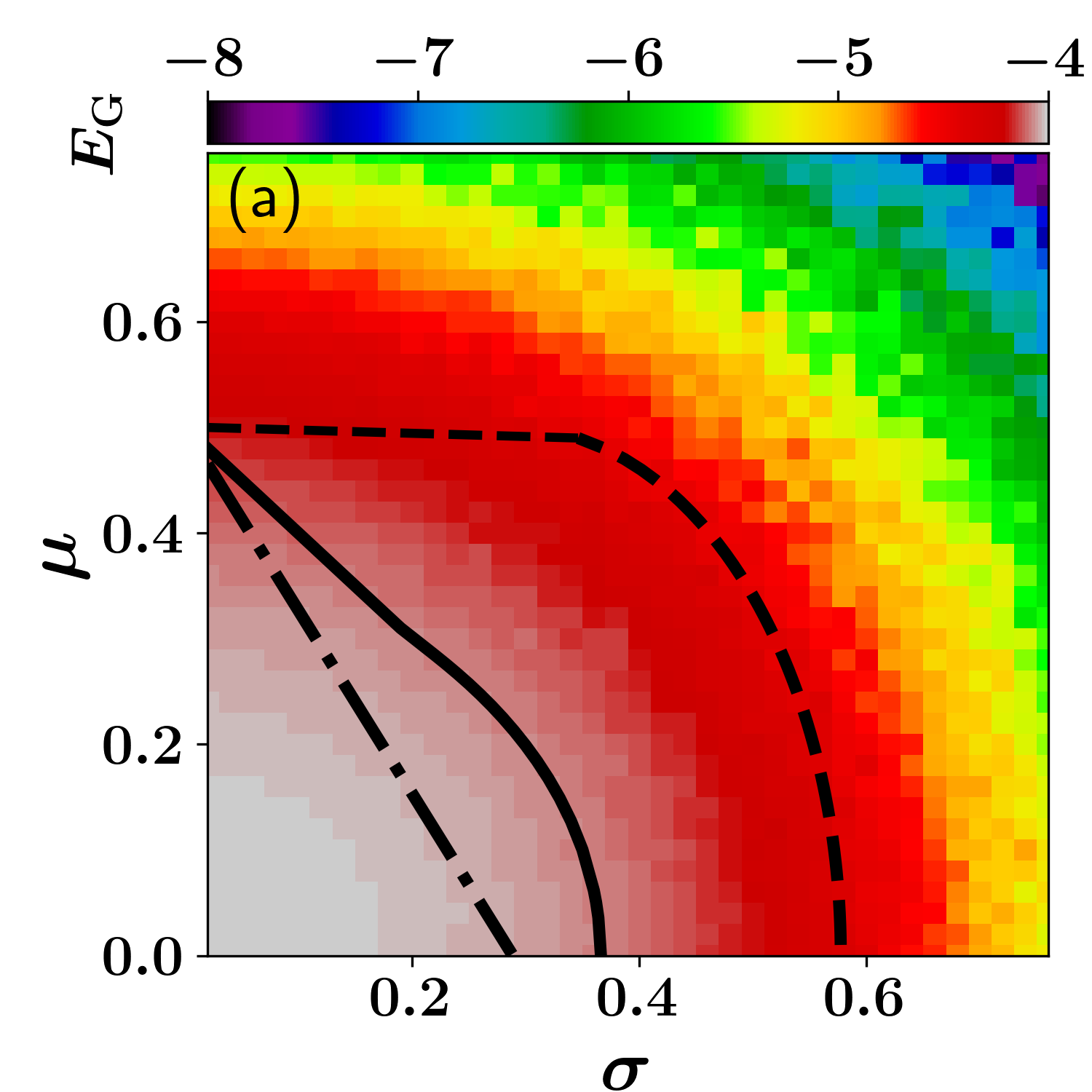
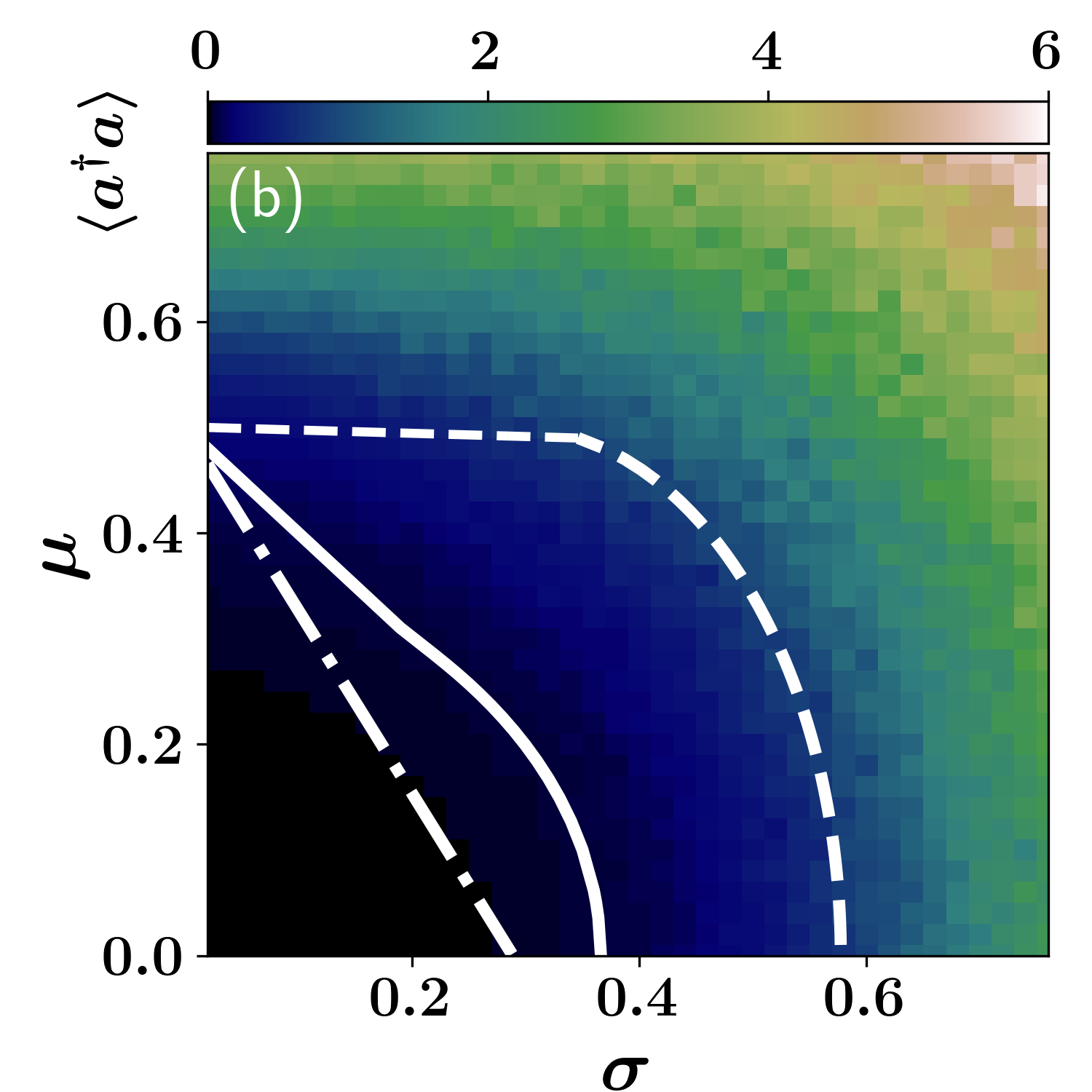
Figure 2: Phase diagram of the disordered Dicke model with uniform coupling distribution (Eq. (6)). To map it out, we show (a) the ground state energy $E_{\text{G}}$ and (b) the average boson number, $\langle a^{\dagger}a\rangle$ wrt. the ground state, as a function of the standard deviation $\sigma$ and the mean $\mu$ of the coupling parameters $g_{i}$. We consider the resonant case: $\omega=\omega_{0}=1$, take the average over $120$ realizations, and fix the atom number to be $N=8$, the bosonic cut-off to be $n_{\text{max}}=40$.

In the first scenario the coupling $g$ is drawn from a uniform distribution:

$$P_{u}(g)=\begin{cases}\frac{1}{2\sqrt{3}\sigma}\quad\textrm{if}\quad\mu-\sqrt{3}\sigma<g<\mu+\sqrt{3}\sigma\\ 0\quad\quad\quad\textrm{otherwise}\end{cases}$$ (6)

with mean $\mu$ and standard deviation $\sigma$.

The disorder-averaged ground state energy and average boson number, are found from the integrals:

$$\overline{E_{G}} =\int_{x_{1}}^{x_{2}}P_{u}(g)E_{G}dg,$$ (7)

$$\overline{\langle a^{\dagger}a\rangle} =\int_{x_{1}}^{x_{2}}P_{u}(g)\langle a^{\dagger}a\rangle dg,$$ (8)

where $E_{G}$ is given in Eqn. 3, $\langle a^{\dagger}a\rangle$ is given in Eq. 4, and we use the overline to denote the disorder average. The lower and upper limits of the box distribution are: $x_{1}=\mu-\sqrt{3}\sigma$ and $x_{2}=\mu+\sqrt{3}\sigma$ respectively and we consider $\mu$ and $\sigma$ to be in the range: $[0,1]$.

For the NP ($|g|\leq g_{c}$) we find (Appendix A):

$$\overline{E_{G}} =-\frac{N\omega_{0}}{2},$$ (9)

$$\overline{\langle a^{\dagger}a\rangle} =0.$$ (10)

On the other hand, for the SP ($|g|>g_{c}$), we have:

$$\overline{E_{G}} =-\frac{N}{2\sqrt{3}\sigma}\left[\frac{x_{2}^{3}}{3}-\frac{g_{c}^{4}}{x_{2}}+\frac{2g_{c}}{3}\right],$$ (11)

$$\overline{\langle a^{\dagger}a\rangle} =\frac{N}{2\sqrt{3}\sigma\omega^{2}}\left[\frac{x_{2}^{3}}{3}+\frac{g_{c}^{4}}{x_{2}}-\frac{4g_{c}^{3}}{3}\right].$$ (12)

Taylor expanding around the critical point $g_{c}$ and considering only the dominant terms, we have:

$$\overline{E_{G}} \approx -\frac{N\omega_{0}}{2}-\frac{AN\omega_{0}}{2}(x_{2}-g_{c})-1.33AN\omega_{0}(x_{2}-g_{c})^{3},$$

$$\overline{\langle a^{\dagger}a\rangle} \approx \frac{AN}{\omega^{2}}(x_{2}-g_{c})^{2}-\frac{0.667AN}{\omega^{2}}(x_{2}-g_{c})^{3},$$ (14)

where $A=\frac{1}{2\sqrt{3}\sigma}$ and $x_{2}$ is the upper limit of the integration $\mu+\sqrt{3}\sigma$. At the critical point the ground state energy is $-\frac{N\omega_{0}}{2}$ and the average boson number is zero, hence we have a relation for the critical line as a function of $\mu$ and $\sigma$:

$$\mu+\sqrt{3}\sigma=\frac{1}{2}.$$ (15)

Fig. 2(a) shows the numerical value of the ground state energy $E_{\text{G}}$ of the system as a function of the standard deviation ($\sigma$) and mean ($\mu$) of the coupling parameter. Our goal is to check the validity of the equation for the critical line marking the QPT (Eq. 15) numerically. In this figure the white/pink color indicates the normal phase where the ground state energy is large and constant, $E_{\text{G}}=-\frac{N\omega_{0}}{2}$ and the other colors represent the super-radiant phase where $E_{\text{G}}$ is decreasing. Similarly Fig. 2(b) shows the average boson number in the ground state of the disordered Dicke model. In the normal phase $\overline{\langle a^{\dagger}a\rangle}\approx 0$ (black color), i.e. there are no excitations in the bosonic mode whereas in the super-radiant phase $\overline{\langle a^{\dagger}a\rangle}$ is finite (other colors), which indicates a macroscopic excitation of the bosonic mode. The dash-dotted line here represents the quantum critical line which is given in Eq. 15 and our numerical data already roughly agrees with this linear relation. It is remarkable that the formula describes the numerical data this well, despite the coarse approximation of just disorder-averaging the clean Dicke model results. Around the critical line the expectation value (with respect to the uniform disorder) of the ground state energy and the average boson number can be represented by the simpler Taylor series in Eq. LABEL:eqn:Egs_avg_dm and Eq. 14 respectively. It is clear that for $\mu=0$, the standard deviation of the disordered Dicke model plays the same role as the coupling parameter $g$ in the usual Dicke model and the critical point is $\sigma_{c}=\frac{g_{c}}{\sqrt{3}}$ within this crude approximation.

Figure 3: Effective distribution containing only positive coupling strengths. The left panel denotes the original distribution, whereas the right panel shows the effective distribution where only the absolute values of the coupling strengths are considered. (a) For $\mu-\sqrt{3}\sigma<0$, the effective mean of the coupling strength is $\langle g\rangle=\frac{\mu+3\sigma^{2}}{2\sqrt{3}\sigma}$ and the effective variance $\langle g^{2}\rangle=\mu^{2}+\sigma^{2}$ hence the effective standard deviation is $\sqrt{\mu^{2}+\sigma^{2}-\frac{(\mu+3\sigma^{2})^{2}}{12\sigma^{2}}}$. (b) For $\mu-\sqrt{3}\sigma\geq 0$ the distribution remain unchanged: the mean and the standard deviation of $g$ are $\mu$ and $\sigma$. For both the cases $A=\frac{1}{2\sqrt{3}\sigma}$.

The line that separates the NP and the SP in Fig. 2 can also be obtained approximately with the aid of a heuristic argument that exploits a symmetry of the Hamiltonian. We observe that the Hamiltonian in Eqn. 1 has the same eigenvalues as one in which any one of the couplings $g_{i}$ is changed to $-g_{i}$. In other words, the eigenvalues of $H(\{g_{j},j\neq i\},g_{i})$ and $H(\{g_{j},j\neq i\},-g_{i})$ are the same. This is a direct consequence of the fact that

$$H(\{g_{j},j\neq i\},-g_{i})=\sigma_{i}^{z}H(\{g_{j},j\neq i\},g_{i})\sigma_{i}^{z}.$$ (16)

Thus when the transformation $T=\sigma_{i}^{z}$ is applied on any eigenstate of the Hamiltonian $H(\{g_{j},j\neq i\},g_{i})$, we would get an eigenstate of the Hamiltonian $H(\{g_{j},j\neq i\},-g_{i})$ with the same eigenvalue. This argument naturally extends to the case when multiple $g_{i}$’s undergo a sign change. Hence we can consider a scenario where all the coupling strengths are made positive, i.e. if there are any negative coupling strengths, we simply take their absolute values. Hence when the lower limit of the uniform distribution $\mu-\sqrt{3}\sigma<0$ the effective distribution is:

$$P_{\textrm{eff}}(g)=\begin{cases}\frac{1}{\sqrt{3}\sigma}\quad\quad\textrm{if}\quad 0<g<-(\mu-\sqrt{3}\sigma)\\ \frac{1}{2\sqrt{3}\sigma}\quad\textrm{if}-(\mu-\sqrt{3}\sigma)<g<(\mu+\sqrt{3}\sigma).\end{cases}$$ (17)

as shown in Fig. 3(a). The effective distribution in this case yields a mean value of $\langle g\rangle=\frac{\mu+3\sigma^{2}}{2\sqrt{3}\sigma}$ and a variance of $\langle g^{2}\rangle=\mu^{2}+\sigma^{2}$ which in turn corresponds to a standard deviation of: $\sqrt{\mu^{2}+\sigma^{2}-\frac{(\mu+3\sigma^{2})^{2}}{12\sigma^{2}}}$. If the lower limit of the distribution $\mu-\sqrt{3}\sigma\geq 0$, the effective distribution remains identical to the original one and its mean and standard deviation remain unchanged as $\mu$ and $\sigma$ (Fig. 3(b)).

To identify the phase transition line heuristically, we argue as follows. We would expect that as more and more of the couplings $g_{i}$ are drawn above $g_{c}$, we would see increasingly dominant effects characteristic of the SP. A coarse way to identify this would be to simply demand that the right most edge of the effective distribution (Eqn. 17) must be above the critical coupling $g_{c}=\frac{1}{2}$, i.e.

$$\mu+\sqrt{3}\sigma=\frac{1}{2},$$ (18)

which is nothing but the crude approximation Eqn. 15 and dot-dashed line in Fig. 2. For a refined result, we demand that the mean of the effective distribution (Eqn. 17) must reach above $g_{c}$

$$\frac{\mu+3\sigma^{2}}{2\sqrt{3}\sigma}=\frac{1}{2},\hskip 11.38109pt\mu<\sqrt{3}\sigma$$

$$\mu=\frac{1}{2},\hskip 8.53581pt\mu\geq\sqrt{3}\sigma.$$ (19)

This is shown by the dashed line in Fig. 2. A less stringent condition is to demand that the mean plus one standard deviation of the effective distribution (Eqn. 17) must reach above $g_{c}$

$$\frac{\mu+3\sigma^{2}}{2\sqrt{3}\sigma}+\sqrt{\mu^{2}+\sigma^{2}-\frac{(\mu+3\sigma^{2})^{2}}{12\sigma^{2}}}=0.5,\hskip 11.38109pt\mu<\sqrt{3}\sigma$$

$$\mu+\sigma=0.5,\hskip 8.53581pt\mu\geq\sqrt{3}\sigma.$$

This is shown by the solid white line in Fig. 2 and appears to be closest to the actual line of separation between the SP and NP.

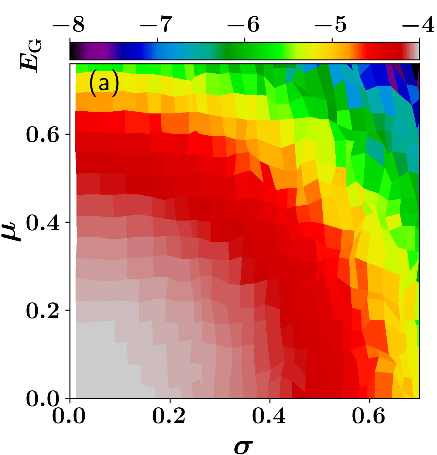
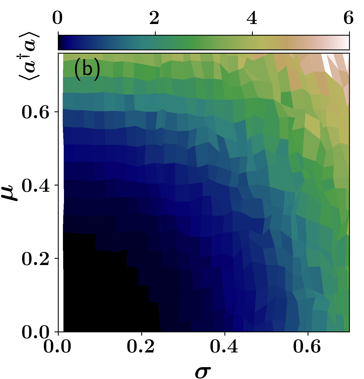
Figure 4: Phase diagram of the disordered Dicke model where $g_{i}=2\cos\theta_{i}$, $\theta_{i}$ are angles randomly drawn from a Gaussian distribution with mean $\theta_{0}$ and standard deviation $\sigma_{\theta}$. To map it out, we show (a) the ground state energy $E_{\text{G}}$ and (b) the average boson number, $\langle a^{\dagger}a\rangle$ wrt. the ground state, as a function of the standard deviation $\sigma$ and the mean $\mu$ of the coupling parameters $g_{i}$. We consider the resonant case: $\omega=\omega_{0}=1$ and take the average over $200$ realizations, and fix the atom number to be $N=8$, and the bosonic cut-off to be $n_{\text{max}}=40$.

III.2 Gaussian distribution

To demonstrate the robustness of our results to variations of the detailed shape of the probability distribution for the coupling, we now consider a second case. The angle $\theta$ is drawn from the Gaussian distribution:

$$P(\theta)\propto e^{-(\theta-\theta_{0})^{2}/\sigma_{\theta}^{2}},$$ (21)

where $\theta_{0}\in[0,\pi]$ is the mean and $\sigma_{\theta}\in[0,\frac{\pi}{4}]$ is the standard deviation of $\theta$ and the disordered coupling strength for the $i^{\text{th}}$ spin is then taken as:

$$g_{i}=2\cos\theta_{i}.$$ (22)

Here, we numerically calculate the mean and the standard deviation of $g$: $\mu=\langle g\rangle=\frac{1}{N}\sum_{i=1}^{N}g_{i}$ and $\sigma=\sqrt{\langle g^{2}\rangle-\langle g\rangle^{2}}$, to obtain characteristics of the distribution that are easily comparable with the previous section. The ground state energy $E_{\text{G}}$ and the average boson number for this distribution are shown in Fig. 4 and we see a behavior similar to the uniform distribution used in Fig. 2.

IV Thermal phase transition

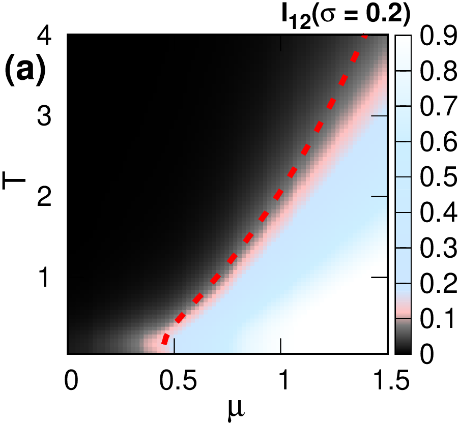
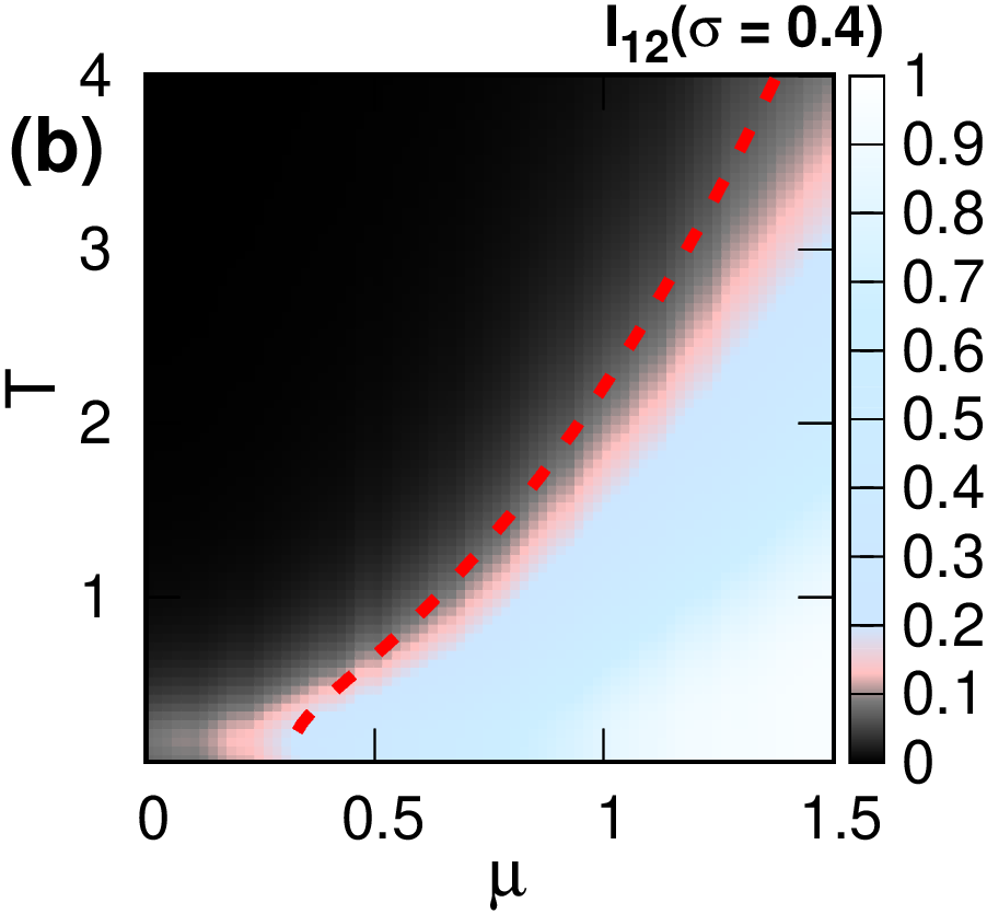
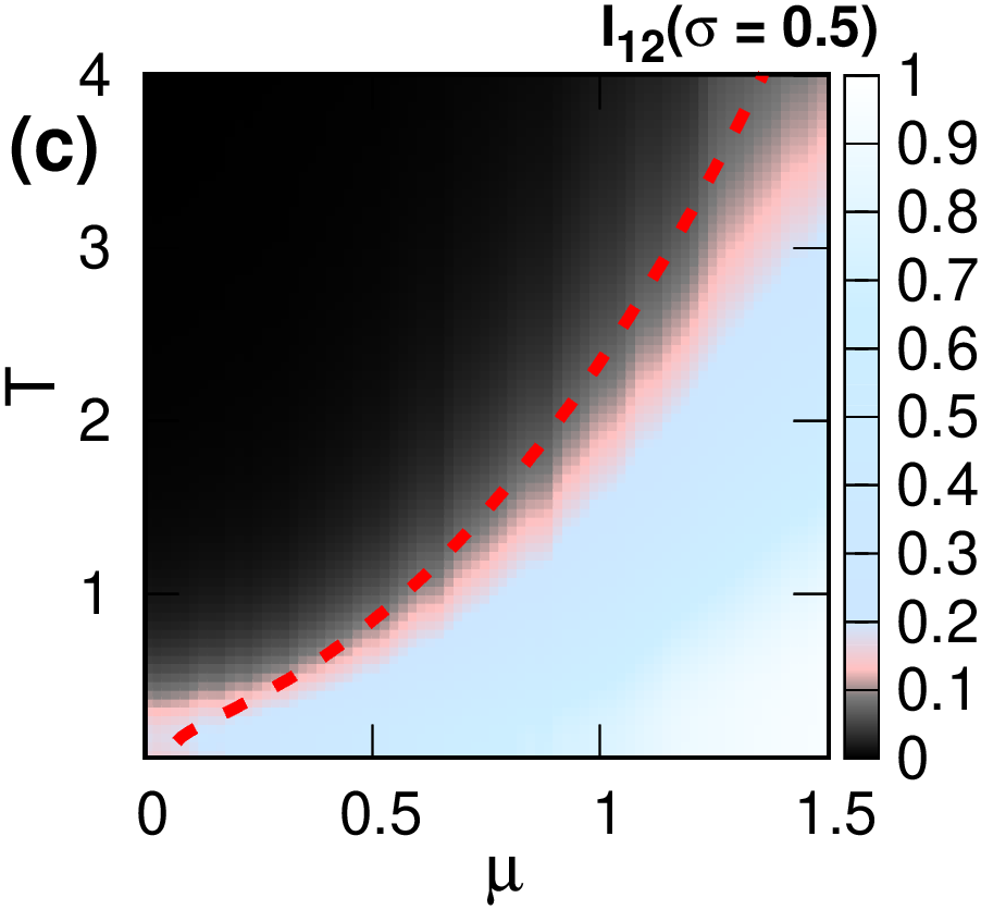
Figure 5: Thermal phase diagrams of the disordered Dicke model, based on the mutual information between two spins. Axes are the temperature $T$ and mean coupling strength $\mu=\langle g\rangle$, for (a) $\sigma=0.2$, (b) $\sigma=0.4$, (c) $\sigma=0.5$, (d) $\sigma=0.8$. The couplings $g$ are drawn from a random uniform distribution with finite mean $\mu$ and standard deviation $\sigma$ (see Eq. 6). The number of atoms is $N=6$ and we choose the bosonic cut-off as $n_{\text{max}}=20$. We take the average over $824$ realizations of $g$ for each $\sigma$.

Moving from the quantum to the thermal phase transition, in this section we derive an analytical expression for the critical temperature for the disordered Dicke model building on previous results [9, 30] for the clean Dicke model. We start by rewriting the system Hamiltonian for the disordered Dicke model as:

$$\tilde{\mathcal{H}} =\frac{\mathcal{H}}{\omega}$$

$$=a^{\dagger}a+\sum_{j=1}^{N}\frac{\epsilon}{2}\sigma_{j}^{z}+\frac{1}{\sqrt{N}}(a+a^{\dagger})\sum_{j=1}^{N}\lambda_{j}\sigma^{x}_{j}$$ (23)

$$=a^{\dagger}a+\sum_{j=1}^{N}h_{j}.$$ (24)

where $\epsilon=\frac{\omega_{0}}{\omega}$, $\lambda_{j}=\frac{g_{j}}{\omega}$ and

$$h_{j} =\frac{\epsilon}{2}\sigma_{j}^{z}+\frac{1}{\sqrt{N}}(a+a^{\dagger})\lambda_{j}\sigma^{x}_{j}.$$ (25)

Following Wang and Hieo [9], who studied the Dicke model within the rotating wave approximation, the partition function can be computed as:

$$Z(N,T)=\sum_{s_{1},...,s_{N}=\pm 1}\int\frac{d^{2}\alpha}{\pi}\langle s_{1}...s_{N}|\langle\alpha|e^{-\beta\tilde{\mathcal{H}}}|\alpha\rangle|s_{1}...s_{N}\rangle$$

$$=\int\frac{d^{2}\alpha}{\pi}e^{-\beta|\alpha|^{2}}\Pi_{j=1,2,...,N}\langle s_{j}|e^{-\beta h_{j}}|s_{j}\rangle$$

$$=\int\frac{d^{2}\alpha}{\pi}e^{-\beta|\alpha|^{2}}\Pi_{j=1,2,...,N}\Big{(}2\cosh\Big{[}\frac{\beta\epsilon}{2}\Big{[}1+\frac{16{\lambda_{j}}^{2}{\alpha}^{2}}{\epsilon^{2}N}\Big{]}^{1/2}\Big{]}\Big{)}.$$ (26)

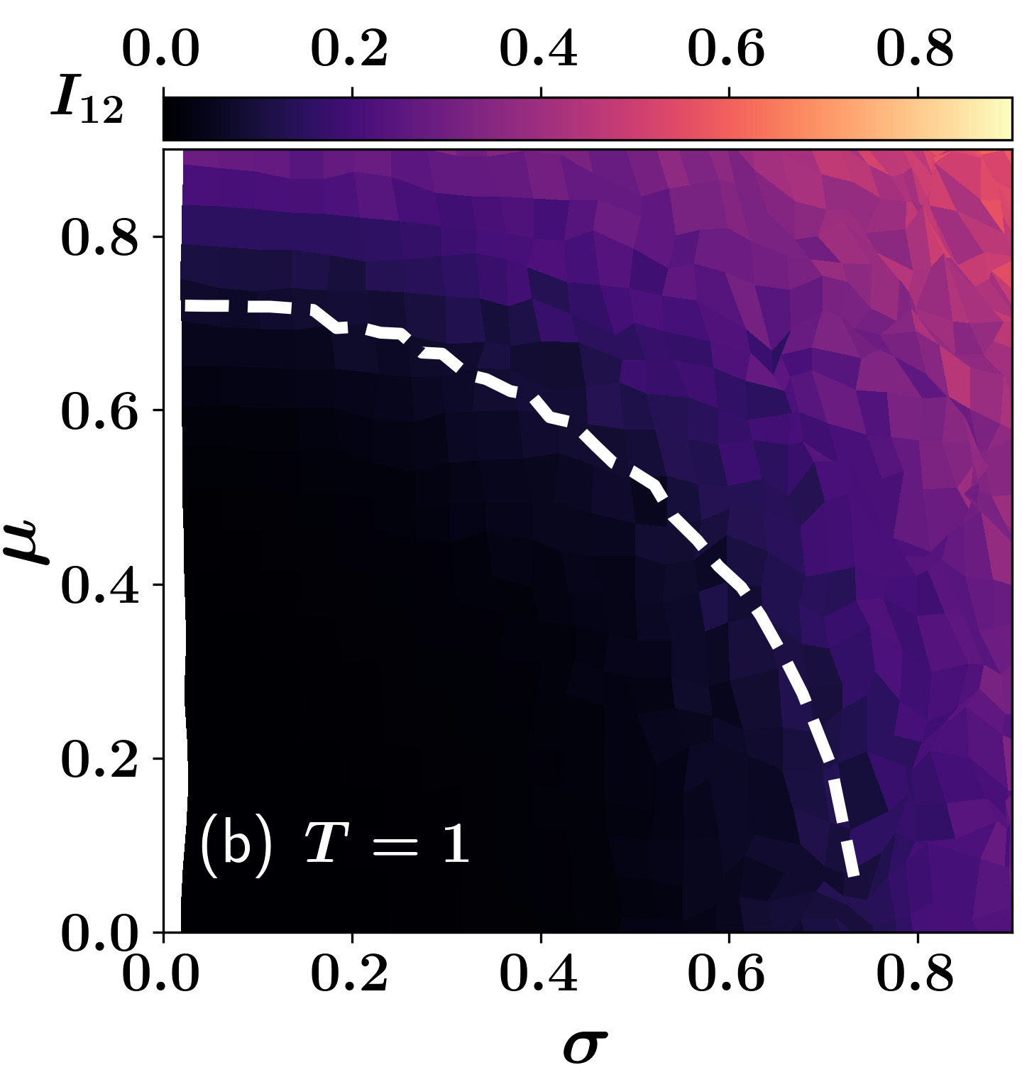
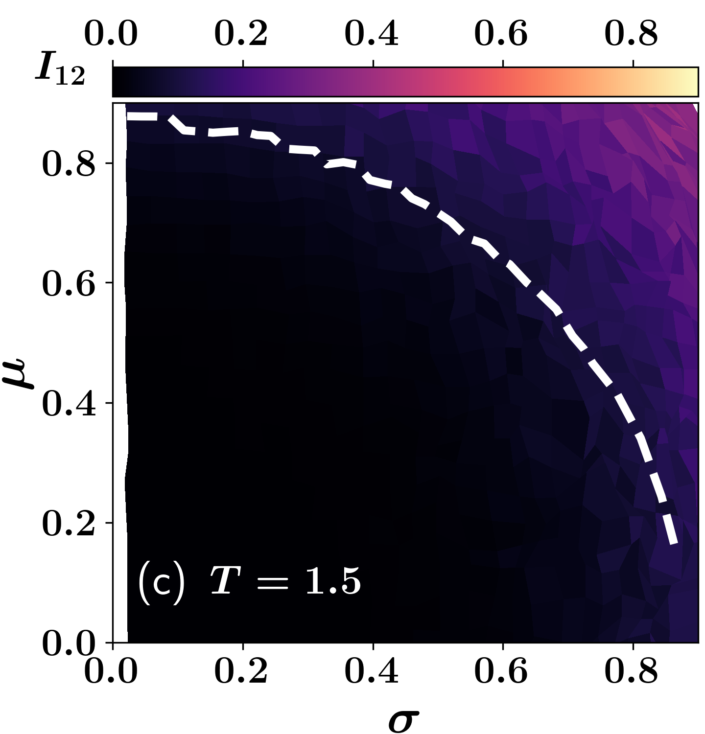
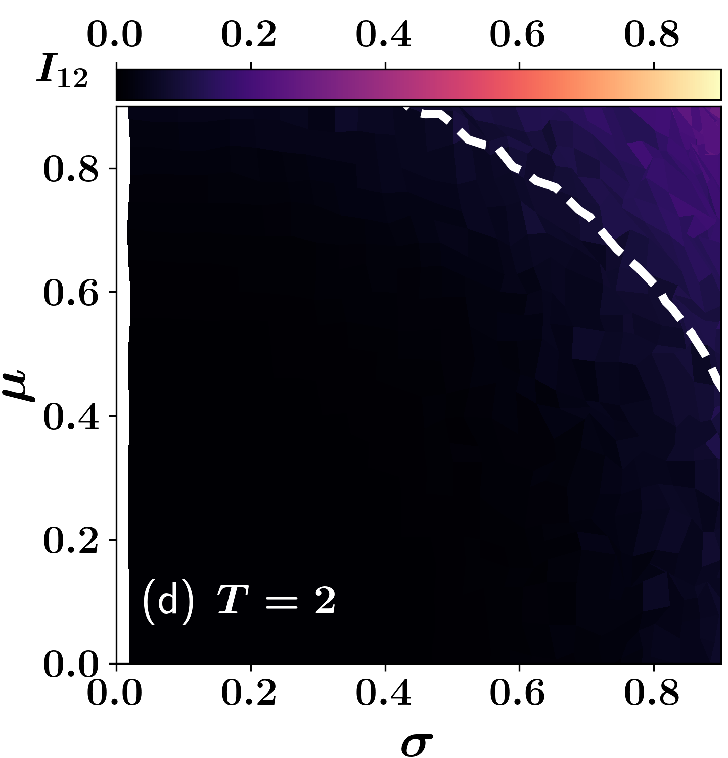
Figure 6: Thermal phase diagrams of the disordered Dicke model, based on the mutual information between two spins. Axes are the standard deviation $\sigma$ and mean coupling strength $\mu=\langle g\rangle$, for (a) $T=0.1$, (b) $T=1$, (c) $T=1.5$, (d) $T=2$. The couplings $g_{i}=2\cos\theta_{i}$, where $\theta_{i}$ are angles randomly drawn from a Gaussian distribution with mean $\theta_{0}$ and standard deviation $\sigma_{\theta}$. The number of atoms is $N=6$ and we choose the bosonic cut-off as $n_{\text{max}}=20$. We take the average over $96$ realizations of $g$ for each temperature.

Here $|\alpha\rangle$ is a coherent state which satisfies the relation: $a|\alpha\rangle=\alpha|\alpha\rangle$ and $|s_{1}...s_{N}\rangle$ is the product basis for the spin subspace. In polar coordinates the partition function becomes:

$$Z(N,T)=\int_{0}^{\infty}rdre^{-\beta r^{2}}\Pi_{j=1,2,...,N}\Big{(}2\cosh\Big{[}\frac{\beta\epsilon}{2}\Big{[}1+\frac{16{\lambda_{j}}^{2}r^{2}}{\epsilon^{2}N}\Big{]}^{1/2}\Big{]}\Big{)}.$$ (27)

Defining the variable $y=\frac{r^{2}}{N}$ allows us to rewrite the above integral as:

$$Z(N,T) =N\int_{0}^{\infty}dye^{-\beta Ny}\Pi_{j=1,2,...,N}\Big{(}2\cosh\Big{[}\frac{\beta\epsilon}{2}\Big{[}1+\frac{16{\lambda_{j}}^{2}y}{\epsilon^{2}}\Big{]}^{1/2}\Big{]}\Big{)}$$

$$=N\int_{0}^{\infty}dy\exp\Big{(}-\beta Ny+\sum_{j=1}^{N}\log\Big{[}\Big{(}2\cosh\Big{[}\frac{\beta\epsilon}{2}\Big{[}1+\frac{16{\lambda_{j}}^{2}y}{\epsilon^{2}}\Big{]}^{1/2}\Big{]}\Big{)}\Big{]}\Big{)}.$$ (28)

We can write this more compactly as

$$Z(N,T) =N\int_{0}^{\infty}dy\exp\Big{(}\phi_{N}(y)\Big{)}$$ (29)

using a shorthand:

$$\phi_{N}(y)=\\ -\beta Ny+\sum_{j=1}^{N}\log\Big{[}\Big{(}2\cosh\Big{[}\frac{\beta\epsilon}{2}\Big{[}1+\frac{16{\lambda_{j}}^{2}y}{\epsilon^{2}}\Big{]}^{1/2}\Big{]}\Big{)}\Big{]}.$$ (30)

for the exponent. We would like to evaluate the above integral using the method of steepest descent for which we would like to extract the point at which $\phi_{N}(y)$ is a maximum. To find this, we compute the derivative:

$$\frac{d\phi_{N}(y)}{dy} =-\beta N+\frac{4\beta}{\epsilon}\sum_{j}\frac{\lambda_{j}^{2}}{\eta_{j}}\tanh\Big{(}\frac{\beta\epsilon\eta_{j}}{2}\Big{)},$$ (31)

where we are using the shorthand notation

$$\eta_{j} =\Big{[}1+\frac{16{\lambda_{j}}^{2}y}{\epsilon}^{2}\Big{]}^{1/2}.$$ (32)

A vanishing derivative, $\frac{d\phi_{N}(y)}{dy}=0$, implies:

$$0 =-\beta N+\frac{4\beta}{\epsilon}\sum_{j}\frac{\lambda_{j}^{2}}{\eta_{j}}\tanh\Big{(}\frac{\beta\epsilon\eta_{j}}{2}\Big{)}.$$ (33)

Following the intuition from the corresponding calculation for the clean Dicke model, we argue that the critical value of the inverse temperature must correspond to the case when all the $\eta_{j}$ take their minimum possible value namely unity. Inserting $\eta_{j}=1$, we have:

$$0 =-\beta_{c}N+\frac{4\beta_{c}}{\epsilon}\sum_{j}\lambda_{j}^{2}\tanh\Big{(}\frac{\beta_{c}\epsilon}{2}\Big{)}$$ (34)

which can be reshaped into

$$\sum_{j}\lambda_{j}^{2}\tanh\Big{(}\frac{\beta_{c}\epsilon}{2}\Big{)} =\frac{N\epsilon}{4}.$$ (35)

This gives us

$$\tanh\Big{(}\frac{\beta_{c}\epsilon}{2}\Big{)} =\frac{\epsilon}{4\frac{\sum\lambda_{j}^{2}}{N}}=\frac{\epsilon}{4\langle\lambda^{2}\rangle}.$$ (36)

Substituting for the expressions for $\epsilon$ and $\lambda$, we obtain an expression for the transition temperature:

$$T_{c} =\frac{\omega_{0}}{2\omega}\frac{1}{\tanh^{-1}\Big{(}\frac{\omega_{0}\omega}{4\langle g^{2}\rangle}\Big{)}}.$$ (37)

To verify this expression for the critical temperature, we numerically study the mutual information between two spins, which has been shown to be a useful marker for the thermal phase transition in the Dicke model [8, 29]. In Fig. 5, we show the mutual information between two spins as a function of the mean coupling strength $\mu$ and the temperature $T$, for different standard deviations: $\sigma=0.2,\ 0.4,\ 0.5,\ 0.8$ . For $\sigma=0.2$ the phase diagram is almost identical to the one for the usual DM (see Fig. 4(c) of our earlier work [8]). For $\mu<\frac{1}{2}$ the system lies in the normal phase, which gives rise here to the black color; for $\mu>\frac{1}{2}$, there is a thermal phase transition from the super-radiant phase (light color) to the normal phase around some critical temperature. In this figure the red dashed line denotes the analytical critical temperature of Eq. 37. We can see that it describes the numerical results well. If the standard deviation is increased, it is clear from Fig. 5 (b) ($\sigma=0.4$) and (c) ($\sigma=0.5$) that the thermal phase transition starts at lower mean values $\mu$ than $\mu=g_{c}$. Finally, for sufficiently wide coupling distributions, with e.g. $\sigma=0.8$, there is a clear TPT from the SP to the NP even for vanishing mean coupling strength $\mu=0.0$. Hence, we can conclude from Fig. 5 that if we introduce disorder with a sufficiently broad distribution into the coupling strength between spins and bosons, there exists a TPT even for vanishing mean coupling $\mu=\langle g\rangle=0$.

In Fig. 6, we show similar data, but using the distribution based on angles, Eq. (21)-Eq. (22). We again show the mutual information between two spins as a function of the mean and the standard deviation of the spin-boson coupling strength for fixed temperatures. Here $\theta$ is a random number, drawn from a Gaussian distribution and $g=2\cos\theta$ which we describe in the subsection III.2. In the normal phase the mutual information is small, shown by black color. On the other hand, in the super-radiant phase $I_{12}$ is relatively high, which is represented by the other colors. One can notice that when we gradually increase the temperature, the normal phase is also expanding in parameter space. In this figure the white dashed curves represent the critical values of $\sigma$ and $\mu$ for TPT that we derived analytically in Eq. (37), which separate the normal and super-radiant phases quite well.

V Realizing disordered couplings in Dicke model with cold atom or ultracold molecules in a cavity

While we intentionally study the abstract model (1) such that it can apply to a variety of systems, we provide in this section some examples for practical realisations. When considering the origin of the Hamiltonian (1) through light matter coupling for two-level systems in a single mode optical cavity, one has, in the dipole approximation [35]

$$g_{i} =\sqrt{\frac{1}{2\hbar\epsilon_{0}\omega}}\omega_{0}u(\mathbf{x}_{i})d_{21}\cos{\theta}_{i},$$ (38)

where $\epsilon_{0}$ is the vacuum permeability, $u(\mathbf{x}_{i})$ the cavity mode amplitude at the location $\mathbf{x}_{i}$ of the $i^{th}$ two level system, and $d_{21}\cos{\theta}_{i}$ the transition dipole matrix element between $|\,{2}\,\rangle$ and $|\,{1}\,\rangle$ projected onto the local cavity field axis, where we have made the dependence on the angle $\theta_{i}$ between cavity field at $\mathbf{x}_{i}$ and transition dipole axis explicit.

Even for identical atoms or molecules, treated as an approximate two-level system (TLS), a random position distribution $\mathbf{x}_{i}$ can now translate into disordered coupling strengths through the position of the TLS relative to the cavity field structure in $u(\mathbf{x}_{i})$ that may contain standing waves, which will cause disorder in the field strength. While this can easily be avoided by trapping all atoms on spatial scales small compared to the cavity wavelength [36], one can just as well generate a range of coupling distributions by weakly trapping the atoms on the flanks of a standing wave [37].

For atomic TLSs without any external fields other than the cavity field, there would be no additional contribution from the transition dipole orientation, since we can always choose the quantisation axis along the local cavity mode electric field direction, such that $\cos{\theta}_{i}\rightarrow 1$. This is no longer true once an additional external field perturbs the symmetry, or the particle is asymmetric, such as most molecules are.

A symmetry breaking field $\mathbf{B}$ could be magnetic, strong enough to Zeeman-shift undesired magnetic sublevels of the excited state out of cavity resonance and locally defining the quantisation axis. If the cavity is penetrated for example by the circular magnetic field around a current carrying wire, a random 3D distribution of atomic positions will translate into a random distribution of angles between quantisation axis and cavity mode electric field, and hence affect couplings, as sketched in Fig. 1.

Another approach to break the symmetry of the two-level system would be considering ultra-cold molecules [38, 39] in the optical cavity [40]. Typical hetero-nuclear molecules possess transition dipole moments with a fixed orientation relative to the molecular axis [41]. Molecules oriented randomly in 3D, such as in the ground state with angular momentum $J=0$ of the quantum mechanical rotor, will thus exhibit a distribution of couplings. Disadvantages of molecules are their vibrational and rotational degrees of freedom, which are undesired here. However eliminating or minimising the impact of these is also required for quantum information and quantum simulation applications of ultra-cold molecules and aids cooling them, and is thus being actively pursued. Coupling to both degrees of freedom can be strongly suppressed, by choosing a molecule with a nearly diagonal Franck-Condon factor [42] between ground and excited state, and a larger angular momentum in the ground state than the excited state [43, 44].

Randomly oriented molecules neatly realise the uniform coupling distribution that we focussed on, since the probability of a given polar angle $\theta$ is $P(\theta)=\frac{\sin\theta}{2}$ and hence $P(\cos\theta)$ will be uniform. Refined distributions can then be tailored by partially orienting molecules along the cavity field axis, e.g. $P(\theta)={\cal N}e^{-(\theta-\theta_{0})^{2}/\sigma_{\theta}^{2}}$, with $\theta_{0}$ enforced by an additional external bias field $\mathbf{E}$ (see Fig. 1).

The implementations of the disordered Dicke model with cold atoms and molecules in cavities that we discussed above can then provide controlled insight, which can be leveraged for understanding the underlying Hamiltonian in more complex and less controlled cases, such as when studying superradiance effects in semi-conductor quantum dot lattices [32]. In this case transition dipoles of carriers in quantum dots are also likely disordered by additional fields and quantum dot geometries, however a clear distinction of such effects from other disorder and decoherence sources will be much more difficult.

VI Summary and conclusions

In this work, we propose and investigate a disordered single-mode Dicke model. We specifically focus on two concrete random distributions of the spin-boson coupling parameters $g_{i}$: (i) a uniform distribution, (ii) $g_{i}\propto\cos\theta_{i}$, where $\theta_{i}$ are Gaussian random variables and study the resulting quantum and thermal phase transitions in the disordered Dicke model. In both cases we see similar results and hence demonstrate that our results are robust to changes in the detailed shape of the distribution.

We find that the phase transitions depend on both the mean and the standard deviation of the random coupling strengths. For the QPT, we find that for mean coupling strengths significantly smaller than their standard deviation $\sigma$, the latter plays a role similar to the coupling $g$ in the clean Dicke model. Even for vanishing mean coupling $\mu=0$, the system thus shows a QPT around $\sigma=\frac{0.5}{\sqrt{3}}$ for uniformly distributed couplings. When $\mu$ is systematically increased, the critical value of $\sigma$ decreases and after a certain mean coupling ($=g_{c}$) the QPT disappears. We derive approximate expressions for the ground state energy and the average boson number around the critical line: $\mu+\sqrt{3}\sigma=\frac{1}{2}$, for the QPT in the $\mu-\sigma$ plane, which provide a reasonably good and simple approximation of our numerical results. Exploiting a symmetry of the Dicke model allows us to improve on the expression.

We also derive an analytical expression for the critical temperature and numerically verify it with the aid of mutual information between two spins. It shows that for wide distributions, such that $\sigma$ is large, there is a phase transition from SP to NP at $\sigma\approx 0.8$ even for vanishing mean coupling strength, $\mu=0$.

The disordered Dicke model should describe quantum dot superlattices in semiconductor quantum optics (see e.g. [32]). Additionally, we list several methods, by which the disordered Dicke model can be realized in experiments with ultracold atoms or molecules in a cavity.

Appendix A The uniform distribution

Consider the scenario where the coupling $g$ is drawn from a uniform distribution:

$$P_{u}(g)=\begin{cases}\frac{1}{2\sqrt{3}\sigma}\quad\textrm{if}\quad\mu-\sqrt{3}\sigma<g<\mu+\sqrt{3}\sigma\\ 0\quad\quad\quad\textrm{otherwise}\end{cases}$$ (39)

with mean $\mu$ and standard deviation $\sigma$.

To calculate the disorder-averaged ground state energy and average boson number, we have to evaluate:

$$\overline{E_{G}} =\int_{x_{1}}^{x_{2}}P_{u}(g)E_{G}dg,$$ (40)

$$\overline{\langle a^{\dagger}a\rangle} =\int_{x_{1}}^{x_{2}}P_{u}(g)\langle a^{\dagger}a\rangle dg,$$ (41)

where $E_{G}$ is given in Eqn. 3 and $\langle a^{\dagger}a\rangle$ is given in Eq. 4. The lower and upper limits of the box distribution are: $x_{1}=\mu-\sqrt{3}\sigma$ and $x_{2}=\mu+\sqrt{3}\sigma$ respectively and we consider $\mu$ and $\sigma$ to be in the range: $[0,1]$. Depending on the relation between $x_{1}$ and $x_{2}$ and $g_{c}$, there are five cases to be considered. After performing the integration outlined above, we obtain an expression for the disorder averaged ground state energy:

$$\overline{E_{G}} =\begin{cases}D_{1}\left[\frac{2g_{c}}{3}-\frac{x_{1}^{3}}{3}+\frac{g_{c}^{4}}{x_{1}}\right]&x_{1}<-g_{c}\ \text{and}\ 0<x_{2}\leq g_{c}\\ D_{1}\left[\frac{4g_{c}^{3}}{3}+\frac{1}{3}\left(x_{2}^{3}-x_{1}^{3}\right)+g_{c}^{4}\left(\frac{1}{x_{1}}-\frac{1}{x_{2}}\right)\right]&x_{1}<-g_{c}\ \text{and}\ x_{2}>g_{c}\\ -\frac{N\omega_{0}}{2}&|x_{1}|<g_{c}\ \text{and}\ 0<x_{2}\leq g_{c}\\ D_{1}\left[\frac{x_{2}^{3}}{3}-\frac{g_{c}^{4}}{x_{2}}+\frac{2g_{c}}{3}\right]&|x_{1}|<g_{c}\ \text{and}\ x_{2}>g_{c}\\ D_{1}\left[\frac{1}{3}\left(x_{2}^{3}-x_{1}^{3}\right)+g_{c}^{4}\left(\frac{1}{x_{1}}-\frac{1}{x_{2}}\right)\right]&x_{1},\ x_{2}>g_{c}\ \text{and}\ \ x_{1}<x_{2}\end{cases}$$ (42)

where $D_{1}=-\frac{N}{2\sqrt{3}\sigma}$. For the average boson number the disorder-averaged expression is:

$$\overline{\langle a^{\dagger}a\rangle} =\begin{cases}D_{2}\left[-\frac{4g_{c}^{2}}{3}-\frac{x_{1}^{3}}{3g_{c}^{2}}-\frac{g_{c}^{4}}{x_{1}}\right]&x_{1}<-g_{c}\ \text{and}\ 0<x_{2}\leq g_{c}\\ D_{2}\left[-\frac{8g_{c}^{3}}{3}+\frac{1}{3}\left(x_{2}^{3}-x_{1}^{3}\right)+g_{c}^{4}\left(\frac{1}{x_{2}}-\frac{1}{x_{1}}\right)\right]&x_{1}<-g_{c}\ \text{and}\ x_{2}>g_{c}\\ 0&|x_{1}|<g_{c}\ \text{and}\ 0<x_{2}\leq g_{c}\\ D_{2}\left[\frac{x_{2}^{3}}{3}+\frac{g_{c}^{4}}{x_{2}}-\frac{4g_{c}^{3}}{3}\right]&|x_{1}|<g_{c}\ \text{and}\ x_{2}>g_{c}\\ D_{2}\left[\frac{1}{3}\left(x_{2}^{3}-x_{1}^{3}\right)+g_{c}^{4}\left(\frac{1}{x_{2}}-\frac{1}{x_{1}}\right)\right]&x_{1},\ x_{2}>g_{c}\ \text{and}\ \ x_{1}<x_{2}\end{cases}$$ (43)

where $D_{2}=\frac{N}{2\sqrt{3}\sigma\omega^{2}}$.

For the NP ($|g|\leq g_{c}$) the third case is applicable and thus:

$$\overline{E_{G}} =-\frac{N\omega_{0}}{2},$$ (44)

$$\overline{\langle a^{\dagger}a\rangle} =0.$$ (45)

On the other hand, for the SP ($|g|>g_{c}$), we consider only the fourth case: $|x_{1}|<g_{c}\ \&\ x_{2}>g_{c}$ for the QPT around $g_{c}$. Thus:

$$\overline{E_{G}} =-\frac{N}{2\sqrt{3}\sigma}\left[\frac{x_{2}^{3}}{3}-\frac{g_{c}^{4}}{x_{2}}+\frac{2g_{c}}{3}\right],$$ (46)

$$\overline{\langle a^{\dagger}a\rangle} =\frac{N}{2\sqrt{3}\sigma\omega^{2}}\left[\frac{x_{2}^{3}}{3}+\frac{g_{c}^{4}}{x_{2}}-\frac{4g_{c}^{3}}{3}\right].$$ (47)

References

- Dicke [1954] R. H. Dicke, Coherence in spontaneous radiation processes, Physical review 93, 99 (1954).
- Emary and Brandes [2003a] C. Emary and T. Brandes, Quantum chaos triggered by precursors of a quantum phase transition: The dicke model, Phys. Rev. Lett. 90, 044101 (2003a).
- Emary and Brandes [2003b] C. Emary and T. Brandes, Chaos and the quantum phase transition in the dicke model, Phys. Rev. E 67, 066203 (2003b).
- Lambert et al. [2004] N. Lambert, C. Emary, and T. Brandes, Entanglement and the phase transition in single-mode superradiance, Phys. Rev. Lett. 92, 073602 (2004).
- Baumann et al. [2010] K. Baumann, C. Guerlin, F. Brennecke, and T. Esslinger, Dicke quantum phase transition with a superfluid gas in an optical cavity, nature 464, 1301 (2010).
- Kirton et al. [2019] P. Kirton, M. M. Roses, J. Keeling, and E. G. Dalla Torre, Introduction to the dicke model: from equilibrium to nonequilibrium, and vice versa, Advanced Quantum Technologies 2, 1800043 (2019).
- Pérez-Fernández and Relaño [2017] P. Pérez-Fernández and A. Relaño, From thermal to excited-state quantum phase transition: The dicke model, Phys. Rev. E 96, 012121 (2017).
- Das and Sharma [2022] P. Das and A. Sharma, Revisiting the phase transitions of the dicke model, Phys. Rev. A 105, 033716 (2022).
- Wang and Hioe [1973] Y. K. Wang and F. T. Hioe, Phase transition in the dicke model of superradiance, Phys. Rev. A 7, 831 (1973).
- Zhu et al. [2019] G.-L. Zhu, X.-Y. Lü, S.-W. Bin, C. You, and Y. Wu, Entanglement and excited-state quantum phase transition in an extended dicke model, Frontiers of Physics 14, 1 (2019).
- Cejnar et al. [2021] P. Cejnar, P. Stránskỳ, M. Macek, and M. Kloc, Excited-state quantum phase transitions, Journal of Physics A: Mathematical and Theoretical 54, 133001 (2021).
- Gross and Haroche [1982] M. Gross and S. Haroche, Superradiance: An essay on the theory of collective spontaneous emission, Physics reports 93, 301 (1982).
- Carmichael et al. [1973] H. Carmichael, C. Gardiner, and D. Walls, Higher order corrections to the dicke superradiant phase transition, Physics Letters A 46, 47 (1973).
- Duncan [1974] G. C. Duncan, Effect of antiresonant atom-field interactions on phase transitions in the dicke model, Phys. Rev. A 9, 418 (1974).
- Quan and Cucchietti [2009] H. T. Quan and F. M. Cucchietti, Quantum fidelity and thermal phase transitions, Phys. Rev. E 79, 031101 (2009).
- Bastarrachea-Magnani et al. [2017] M. A. Bastarrachea-Magnani, A. Relaño, S. Lerma-Hernández, B. L. del Carpio, J. Chávez-Carlos, and J. G. Hirsch, Adiabatic invariants for the regular region of the dicke model, Journal of Physics A: Mathematical and Theoretical 50, 144002 (2017).
- Temnov and Woggon [2005] V. V. Temnov and U. Woggon, Superradiance and subradiance in an inhomogeneously broadened ensemble of two-level systems coupled to a low- cavity, Phys. Rev. Lett. 95, 243602 (2005).
- Marchetti et al. [2006] F. M. Marchetti, J. Keeling, M. H. Szymańska, and P. B. Littlewood, Thermodynamics and excitations of condensed polaritons in disordered microcavities, Phys. Rev. Lett. 96, 066405 (2006).
- Marchetti et al. [2007] F. M. Marchetti, J. Keeling, M. H. Szymańska, and P. B. Littlewood, Absorption, photoluminescence, and resonant rayleigh scattering probes of condensed microcavity polaritons, Phys. Rev. B 76, 115326 (2007).
- Diniz et al. [2011] I. Diniz, S. Portolan, R. Ferreira, J. M. Gérard, P. Bertet, and A. Auffèves, Strongly coupling a cavity to inhomogeneous ensembles of emitters: Potential for long-lived solid-state quantum memories, Phys. Rev. A 84, 063810 (2011).
- Tsyplyatyev and Loss [2009] O. Tsyplyatyev and D. Loss, Dynamics of the inhomogeneous dicke model for a single-boson mode coupled to a bath of nonidentical spin-1/2 systems, Phys. Rev. A 80, 023803 (2009).
- Dhar et al. [2018] H. S. Dhar, M. Zens, D. O. Krimer, and S. Rotter, Variational renormalization group for dissipative spin-cavity systems: Periodic pulses of nonclassical photons from mesoscopic spin ensembles, Phys. Rev. Lett. 121, 133601 (2018).
- Krimer et al. [2014] D. O. Krimer, S. Putz, J. Majer, and S. Rotter, Non-markovian dynamics of a single-mode cavity strongly coupled to an inhomogeneously broadened spin ensemble, Phys. Rev. A 90, 043852 (2014).
- Krimer et al. [2016] D. O. Krimer, M. Zens, S. Putz, and S. Rotter, Sustained photon pulse revivals from inhomogeneously broadened spin ensembles, Laser & Photonics Reviews 10, 1023 (2016).
- Zhang et al. [2018] Z. Zhang, C. H. Lee, R. Kumar, K. J. Arnold, S. J. Masson, A. L. Grimsmo, A. S. Parkins, and M. D. Barrett, Dicke-model simulation via cavity-assisted raman transitions, Phys. Rev. A 97, 043858 (2018).
- Vedral [2003] V. Vedral, Classical correlations and entanglement in quantum measurements, Phys. Rev. Lett. 90, 050401 (2003).
- DiVincenzo et al. [2004] D. P. DiVincenzo, M. Horodecki, D. W. Leung, J. A. Smolin, and B. M. Terhal, Locking classical correlations in quantum states, Phys. Rev. Lett. 92, 067902 (2004).
- Adesso and Datta [2010] G. Adesso and A. Datta, Quantum versus classical correlations in gaussian states, Phys. Rev. Lett. 105, 030501 (2010).
- Das et al. [2023] P. Das, D. S. Bhakuni, and A. Sharma, Phase transitions of the anisotropic dicke model, Phys. Rev. A 107, 043706 (2023).
- Hioe [1973] F. T. Hioe, Phase transitions in some generalized dicke models of superradiance, Phys. Rev. A 8, 1440 (1973).
- Rotondo et al. [2015] P. Rotondo, M. Cosentino Lagomarsino, and G. Viola, Dicke simulators with emergent collective quantum computational abilities, Phys. Rev. Lett. 114, 143601 (2015).
- Rainò et al. [2018] G. Rainò, M. A. Becker, M. I. Bodnarchuk, R. F. Mahrt, M. V. Kovalenko, and T. Stöferle, Superfluorescence from lead halide perovskite quantum dot superlattices, Nature 563, 671 (2018).
- Dimer et al. [2007] F. Dimer, B. Estienne, A. S. Parkins, and H. J. Carmichael, Proposed realization of the dicke-model quantum phase transition in an optical cavity qed system, Phys. Rev. A 75, 013804 (2007).
- Maziero et al. [2010] J. Maziero, H. Guzman, L. Céleri, M. Sarandy, and R. Serra, Quantum and classical thermal correlations in the xy spin-1 2 chain, Phys. Rev. A 82, 012106 (2010).
- Dowling and Milburn [2003] J. P. Dowling and G. J. Milburn, Quantum technology: the second quantum revolution, Philosophical Transactions of the Royal Society of London. Series A: Mathematical, Physical and Engineering Sciences 361, 1655 (2003).
- Neuzner et al. [2016] A. Neuzner, M. Körber, O. Morin, S. Ritter, and G. Rempe, Interference and dynamics of light from a distance-controlled atom pair in an optical cavity, Nature Photonics 10, 303 (2016).
- Puppe et al. [2007] T. Puppe, I. Schuster, A. Grothe, A. Kubanek, K. Murr, P. W. H. Pinkse, and G. Rempe, Trapping and observing single atoms in a blue-detuned intracavity dipole trap, Phys. Rev. Lett. 99, 013002 (2007).
- Krems [2005] R. V. Krems, Molecules near absolute zero and external field control of atomic and molecular dynamics, International Reviews in Physical Chemistry 24, 99 (2005).
- Carr et al. [2009] L. D. Carr, D. DeMille, R. V. Krems, and J. Ye, Cold and ultracold molecules: science, technology and applications, New Journal of Physics 11, 055049 (2009).
- Herrera and Spano [2016] F. Herrera and F. C. Spano, Cavity-controlled chemistry in molecular ensembles, Phys. Rev. Lett. 116, 238301 (2016).
- Badankó et al. [2018] P. Badankó, G. J. Halász, L. S. Cederbaum, Á. Vibók, and A. Csehi, Communication: Substantial impact of the orientation of transition dipole moments on the dynamics of diatomics in laser fields, The Journal of Chemical Physics 149, 181101 (2018).
- Hao et al. [2019] Y. Hao, L. F. Pašteka, L. Visscher, P. Aggarwal, H. L. Bethlem, A. Boeschoten, A. Borschevsky, M. Denis, K. Esajas, S. Hoekstra, et al., High accuracy theoretical investigations of CaF, SrF, and BaF and implications for laser-cooling, The Journal of chemical physics 151, 034302 (2019).
- Stuhl et al. [2008] B. K. Stuhl, B. C. Sawyer, D. Wang, and J. Ye, Magneto-optical trap for polar molecules, Phys. Rev. Lett. 101, 243002 (2008).
- Shuman et al. [2010] E. S. Shuman, J. F. Barry, and D. DeMille, Laser cooling of a diatomic molecule, Nature 467, 820 (2010).