Parallel-in-time quantum simulation via Page and Wootters quantum time

Abstract

In the past few decades, researchers have created a veritable zoo of quantum algorithm by drawing inspiration from classical computing, information theory, and even from physical phenomena. Here we present quantum algorithms for parallel-in-time simulations that are inspired by the Page and Wooters formalism. In this framework, and thus in our algorithms, the classical time-variable of quantum mechanics is promoted to the quantum realm by introducing a Hilbert space of “clock” qubits which are then entangled with the “system” qubits. We show that our algorithms can compute temporal properties over $N$ different times of many-body systems by only using $\log(N)$ clock qubits. As such, we achieve an exponential trade-off between time and spatial complexities. In addition, we rigorously prove that the entanglement created between the system qubits and the clock qubits has operational meaning, as it encodes valuable information about the system’s dynamics. We also provide a circuit depth estimation of all the protocols, showing an exponential advantage in computation times over traditional sequential in time algorithms. In particular, for the case when the dynamics are determined by the Aubry–Andre model, we present a hybrid method for which our algorithms have a depth that only scales as $\mathcal{O}(\log(N)n)$. As a by product we can relate the previous schemes to the problem of equilibration of an isolated quantum system, thus indicating that our framework enable a new dimension for studying dynamical properties of many-body systems.

I Introduction

The field of quantum foundations studies the fundamental principles of quantum theory, such as the nature of quantum states, the interpretation of measurements, the equilibration and thermalization of isolated systems, and the emergence of classicallity [1, 2, 3, 4, 5]. Another important question that has recently attracted wide attention within this field is that of the role of time in quantum mechanics (QM) [6, 7, 8, 9, 10, 11, 12, 13, 14, 15, 16, 17, 18, 19, 20, 21, 22, 23, 24, 25, 26, 27, 28, 29, 30, 31, 32]: It is clear that ever since its inception, time in QM has been treated as an external classical parameter, in asymmetry with other quantum observables. For instance, in the canonical quantization procedure, one promotes the position and momentum variables to operators and the Poisson bracket to a commutator [33]. This quantization is implemented at a fixed time value so the variable $t$ appearing in Schrödinger equation is the same as that appearing in the classical equations of motion. While seemingly innocuous, it is believed that the imbalance between time and space could be a critical issue in developing a quantum theory of gravity [34, 35, 36]. At the same time, such asymmetry inevitably limits the range of applicability of quantum information and computation tools, as asking questions like “what is the entanglement between the space and time coordinates?” is an entirely moot point within the conventional quantum mechanical framework.

It is tempting to fix the space-time asymmetry by promoting $i\hbar\frac{d}{dt}$ to a quantum operator conjugate to some quantum time observable $T$, such that $[T,H]=i\hbar$. However, the previous approach has the critical issue that it forces $T$ and $H$ to have exactly the same eigenspectrum, which is generally incompatible (such argument is often attributed to Pauli [37]). Despite this apparent difficulty and other subtleties, there are several proposals to treat time on equal footing with other physical quantities [38, 39, 40, 41, 42, 13, 14]. Here we will focus on the so-called Page and Wooters (PaW) mechanism [38]. In this framework the universe is composed by a quantum system of interest plus an ancillary clock quantum system, such that the joint state of the universe, the history state, is in a stationary state. The previous “Pauli’s objection” is circumvented since the operator $T$ acts on the clock system implying $[T,H]=0$. Remarkably, as long as the system and the clock are correlated in a specific way, the unitary evolution of the system can be restored by conditioning over the clock states. In this way, measures of system-time entanglement become rigorous quantifiers of the amount of distinguishable evolution undergone by the system during its history [8].

The foundational discussion surrounding the role of time has many intriguing ramifications, even when focusing solely on the PaW mechanism. The interested reader can refer to the Appendix A for pertinent discussions. However, the primary objective of this work is computational: In this manuscript, we provide a translation of the PaW mechanism into a useful quantum computational scheme where the quantum aspects of time are captured by clock qubits. This allows us to develop quantum algorithms for studying temporal averages of several dynamical properties of a quantum system. Specifically, given an $n$-qubit quantum system that is evolving under the action of a time-independent Hamiltonian $H$, we consider the problem of approximating the infinite-time average of some time-dependent dynamical quantity by a discrete sum over $N$ different times. In a standard setting, we can estimate said discrete average by sequentially running $N$ different quantum circuits (one for each time in the average). However, by leveraging the history state of the Page and Wooters formalism we propose a quantum algorithm for parallel-in-time simulations that uses $\log(N)$ (any logarithm in this manuscript is taken in base $2$) ancillary clock qubits and that allows us to evaluate the temporal average with a single quantum circuit. The previous shows that using the history state leads to an exponential trade-off between temporal complexity (running multiple circuits) and spatial complexity (using more qubits).

In addition, we also show that the entanglement between the system and the clock qubits carries operational meaning since it serves as a bound for the infinity time average of the Loschmidt echo and for the temporal variance of expectation values. These results imply that the history state encodes valuable information in its correlations that can be used to study and understand the system’s dynamics and equilibration. Given this operational meaning of the entanglement, we present two different schemes to compute the linear entropy of the history state, one based on the state-overlap circuit [43], and another one leveraging classical shadows and randomized measurements [44, 45]

We also present a depth study of the circuits showing a clear advantage of using parallel-in-time protocols over the conventional sequential-in-time approaches where time is not mapped to clock qubits. Moreover, we propose a scheme to further reduce the circuit depth needed to prepare the history state via Hamiltonian diagonalization [46, 47]. Here, we show that by leveraging tools from variational quantum algorithms [48, 49] and quantum machine learning [50, 51, 52] to variationally diagonalize $H$, one can significantly further reduce the required circuit depth. For the special case when $H$ is given by the Aubry–Andre model, we show that all of our algorithms can be implemented with a depth that only scales as $\mathcal{O}(\log(N)n)$, i.e., as the product of the number of clock and system qubits. Finally, we perform simulations which showcase the performance of our algorithms for studying temporal averages of systems evolving under an Aubry–Andre model.

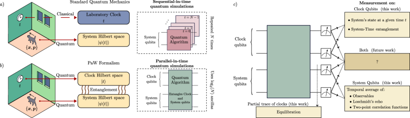
Figure 1: Quantum algorithms based on the standard quantum mechanics or the PaW formalism. a) In Hamiltonian classical mechanics, dynamical variables are functions of the phase space coordinates position $\bm{x}$ and momentum $\bm{p}$. In standard quantum mechanics, one promotes $\bm{x}$ and $\bm{p}$ to quantum operators, but the time variable $t$ is treated as a classical parameter that is external to the quantum system being studied. Quantum algorithms for studying dynamical properties based on this framework are implemented for some fixed time $t$. If we want to compute an average of $N$ times, we need to repeat the run $N$ different sequential-in-time experiments. b) In the PaW formalism, time is treated as a quantum variable, with its own associated Hilbert space. In this work we present quantum algorithms for parallel-in-time simulations which trade circuit repetitions for ancilla clock qubits. c) After a proper entangling protocol one has access not only to properties of the system at a given time, but also to their complete history. This information can be retrieved by performing measurements at the end of the circuit, which now can involve either the clock qubits, the system qubits or both. Measurements on the system which are conditioned to a certain time value give properties of the system at a given time. More interestingly, if one only measures on the system and complete ignore the clock’s values, temporal averages are obtained. This is a consequence of the entanglement between the system and the clock which induces a useful quantum channel when the clock is treated as an environment. Because of the quantum nature of the simulated clock and system, many other measurements can be proposed, meaning that the different protocols we discuss in this manuscript do not exhaust all the possibilities opened by this computational framework.

II Quantum time formalism and its discretization

Let us consider an $n$-qubit quantum system with associated Hilbert space $\mathcal{H}_{S}$. Then, let $H$ be a time-independent Hamiltonian under which the system evolves. The dynamical evolution of the system is determined by the Schrödinger equation

$$i\frac{d}{dt}\ket{\psi(t)}=H\ket{\psi(t)}\,,$$ (1)

where we have set $\hbar=1$. It is well known that the solution of Eq. (1) is given by

$$\ket{\psi(t)}=U(t)\ket{\psi_{0}}\,,\quad\text{with}\quad U(t)=e^{-iHt}\,,$$ (2)

and where $\ket{\psi_{0}}$ is some initial state of the system.

As previously discussed, and as shown in Fig. 1(a), there exists an inherent asymmetry between the space and time variables in quantum mechanics. Namely, the $t$ variable over which we take a derivative is a fully classical parameter that is external to the quantum system. An alternative to fully incorporate time in a quantum framework is to introduce a new Hilbert space $\mathcal{H}_{T}$ spanned by some states $|t\rangle$ (see Fig. 1(b)) such that $T|t\rangle=t|t\rangle$ and $[T,P_{T}]=i\hbar$, which in the time basis leads to $P_{T}\equiv-i\hbar\frac{d}{dt}$. Note that $P_{T}$ is not the Hamiltonian of the system and in fact $[T,H]=0$ (as they act on distinct Hilbert spaces). Evolution is then recovered from an extended Schrodinger equation, involving both the system and the clock Hilbert spaces, which is given by $\mathcal{J}|\Psi\rangle=0$, for $\mathcal{J}=P_{T}\otimes\openone_{S}+\openone_{T}\otimes H$ and $|\Psi\rangle\in\mathcal{H}_{T}\otimes\mathcal{H}_{S}$. Here $\openone_{T}$ and $\openone_{S}$ respectively denote the identities on $\mathcal{H}_{T}$ and $\mathcal{H}_{S}$. In general, the extended Schrodinger equation, together with an initial condition, leads to entanglement between the system and the time Hilbert space.

The previous scheme can also be regarded as the mathematical basis of the Page and Wootters (PaW) mechanism. Under this framework the universe state $|\Psi\rangle$ is stationary (as $\mathcal{J}|\Psi\rangle=0$) while the unitary evolution of the subsystem $S$ emerges by conditioning on the rest. In our previous notation this means that given a universe state

$$|\Psi\rangle=\int dt\,\ket{t}|\psi(t)\rangle\,,$$ (3)

we can recover the state of the system as $|\psi(t)\rangle=\langle t|\Psi\rangle$ (assuming $\langle t|t^{\prime}\rangle=\delta(t-t^{\prime})$). More notably, one can readily see that $\mathcal{J}|\Psi\rangle=(i\partial_{t}-H)|\psi(t)\rangle=0$ precisely recovers the standard Schödinger equation with the index $t$ being demoted from a quantum state label to a time parameter.

In order to make the states $|\Psi\rangle$ accessible to conventional (discrete) qubit-based quantum computers, one needs a proper discrete time framework. Fortunately, it is easy to guess the form of a discrete time history state. Namely, we start by introducing a finite dimensional Hilbert space $\mathcal{H}_{T}$, which we denote as the time or clock-Hilbert space with basis $|t\rangle$ satisfying $\langle t^{\prime}|t\rangle=\delta_{tt^{\prime}}$ for $t=0,\dots,N-1$. A discrete history state is then defined as the state

$$|\Psi\rangle=\frac{1}{\sqrt{N}}\sum_{t=0}^{N-1}|t\rangle|\psi(\varepsilon t)\rangle\,,$$ (4)

with $|\psi(\varepsilon t)\rangle=U(\varepsilon t)|\psi_{0}\rangle\in\mathcal{H}_{S}$. Here, we have $\varepsilon=T/N$ the time-spacing for a given time-window $T$, while $t$ denotes a discrete dimensionless index (so that $\varepsilon t$ is a physical time interval).

In analogy with the continuum case one can recover the state of the system at a given time by conditioning as $|\psi(\varepsilon t)\rangle\langle\psi(\varepsilon t)|={\rm Tr}_{T}[|\Psi\rangle\langle\Psi|\Pi_{t}]/\langle\Psi|\Pi_{t}|\Psi\rangle$ for $\Pi_{t}=|t\rangle\langle t|\otimes\openone_{S}$. In this way the unitarily evolved state is recovered for the time values allowed by $\mathcal{H}_{T}$. Notice that this operation is different from a direct partial trace over the clock states which generally yields a mixed state. It turns out that the partial trace induces a quantum channel which also encodes useful information about the system’s dynamics and its (eventual) equilibration. In fact, one can think about the history states as a purification of that particular quantum channel. This is related to the system-time entanglement as we discuss in Section IV and Appendix B.

Here we note that for the case of $N$ being a power of two, the discrete history state can be prepared with the quantum phase estimation-like circuit of Fig. 2. For $N$ being a power of two, one requires $\log(N)$ ancillary or clock qubits (we henceforth assume the logarithms to be base 2). As such, the clock Hilbert space $\mathcal{H}_{T}$ is of dimension $\dim(\mathcal{H}_{T})=2^{\log(N)}=N$. This result has been reported recently in [8] and [9], where the discrete history state of Eq. (4) has also been extensively studied.

The advantages of encoding history states in a quantum computer become clear once one starts considering measurements on the end of the circuit which are different from simple conditioning: while conditioned measurements allow one to recover properties of the system at a given time, new genuinely quantum possibilities become accessible through the clock qubits. A small summary of such possibilities is provided in Fig. 1(c).

III From qubit-clocks to parallel-in-time simulations

Here we discuss how the mathematical formalism of qubit-clocks presented in the previous section can be leveraged to create novel quantum algorithms aimed at studying averages of dynamical-in-time properties of quantum systems. In particular, in this section we focus in developing parallel-in-time-type algorithms that estimate time averages of physical quantities.

Figure 2: Circuit for preparing history states. As shown above, the initial state to the clock qubits is $\ket{0}^{\otimes\log(N)}$ while that of the system is $\ket{\psi_{0}}$. The action of the Hadamard gates is to map the initial state to $\ket{+}^{\otimes\log(N)}\otimes\ket{\psi_{0}}$. Here, we find it convenient to write $\ket{+}^{\otimes\log(N)}=\frac{1}{\sqrt{N}}\otimes_{j=1}^{\log{N}}(\ket{0_{j}}+\ket{1_{j}})=\frac{1}{\sqrt{N}}\sum_{t=0}^{N-1}\ket{t}$ where we have expressed $t$ in its binary form $t=\sum_{j=1}^{\log{N}}t_{j}2^{j-1}$. Next, the $\log{N}$ controlled gates $U(2^{j-1}\frac{T}{N})=U(\frac{T}{N})^{2^{j-1}}$ for $j=1,\ldots,\log{N}$ perform the operations $U(\varepsilon t)\ket{\psi_{0}}=\ket{\psi(\varepsilon t)}$ for $U(\varepsilon t)=U(\frac{T}{N})^{\sum_{j=1}^{\log{N}}t_{j}2^{j-1}}$.

III.1 Setting

Given a time-independent Hamiltonian $H$ acting on $n$-qubits, and its associated time evolution operator $U(t)=e^{-iHt}$, we consider the problem of estimating general quantities of the form

$$\overline{F}(O_{1},O_{2},\omega) =\lim_{T\rightarrow\infty}\int_{0}^{T}\frac{dt}{T}e^{-i\omega t}\langle O_{1}(t)O_{2}\rangle_{\rho}$$ (5)

$$=\lim_{T\rightarrow\infty}\int_{0}^{T}\frac{dt}{T}e^{-i\omega t}\Tr[\rho O_{1}(t)O_{2}]\,,$$ (6)

where $O_{1}(t)=U^{\dagger}(t)O_{1}U(t)$. Here, $\rho$ is an $n$-qubit state acting on the $d$-dimensional Hilbert space $\mathcal{H}_{S}$ (with $d=2^{n}$), $O_{1}$ and $O_{2}$ are two operators, and $\omega\in\mathbb{R}$.

To illustrate the relevance of the quantity $\overline{F}(\rho,O_{1},O_{2},\omega)$ in Eq. (5) let us consider several special cases. First, let $\omega=0$ and $O_{2}=\openone$, which leads to

$$\overline{F}(O_{1}) :=\overline{F}(O_{1},\openone,0)$$

$$=\lim_{T\rightarrow\infty}\int_{0}^{T}\frac{dt}{T}\langle O_{1}(t)\rangle_{\rho}\,.$$ (7)

We can see that $\overline{F}(\rho,O_{1})$ simply corresponds to an infinite temporal average of the observable $O_{1}$. These quantities are crucial to understanding the dynamical properties of closed quantum systems and in particular their equilibration [4, 53, 54]. They are also relevant to the study of quantum quench processes in field theories [55] and signatures of non-equilibrium quantum phase transition through infinite-time averages of Loschmidt echos [56, 57, 58, 59, 60]. Next, when $\omega=0$, we have

$$\overline{F}(O_{1},O_{2}) :=\overline{F}(O_{1},O_{2},0)$$

$$=\lim_{T\rightarrow\infty}\int_{0}^{T}\frac{dt}{T}\langle O_{1}(t)O_{2}\rangle_{\rho}\,.$$ (8)

Here we can recognize $\langle O_{1}(t)O_{2}\rangle_{\rho}$ as a two-point correlation function (also known as a dynamical Green’s function). Two-point correlation functions are used to describe the behavior of a system under perturbations, and are a widely used tool in quantum many-body systems and condensed matter physics [61, 62, 63, 64]. The infinite-time average of $\langle O_{1}(t)O_{2}\rangle_{\rho}$ has been recently considered in [65] to study thermodynamics properties of closed quantum systems such as the emergence of dissipation at late times.

Finally, we note that the general function $\overline{F}(O_{1},O_{2},\omega)$ corresponds to a Fourier transform of the two-point correlation function, which is commonly referred to as the dynamical structure factor in the condensed matter community [66, 67]. Crucially, the dynamical structure factors are used to study dynamical properties of a given system and have the properties of being experimentally accessible [68, 69], and usually being hard to compute via classical simulations [67].

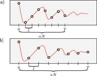
Figure 3: Trade-off between accuracy and resolution. Consider the approximation of the infinite-time average of Eq. (5) given by the discrete sum in Eq. (9). For some fix number of time-steps $N$, there exists a trade-off between the window size $\varepsilon$ and the final time $T$. Namely, larger $T$ implies larger window size $\varepsilon$, and hence less accuracy. On the other hand, smaller final time $T$ implies more resolution in the temporal average at the cost of less accuracy.

While the importance of Eq. (5) is clear, the computation of $\overline{F}(O_{1},O_{2},\omega)$ might not be straightforward. On the one hand, the classical simulation of some quantum mechanical dynamical process is generally expected to be exponentially expensive in classical computers. Such scaling can be mitigated by using a quantum computer. Here, there are several schemes capable of computing fixed-time quantities of the form $\langle O_{1}(t)O_{2}\rangle_{\rho}$  [66, 70, 71, 72]. Still, the issue remains that one needs to perform the time average. In practice, this can be achieved via the discrete-time approximation

$$\widetilde{F}(O_{1},O_{2},\omega) =\frac{1}{N}\sum_{t=0}^{N-1}e^{-i\omega\varepsilon t}\langle O_{1}(\varepsilon t)O_{2}\rangle_{\rho}\,,$$ (9)

where we have $\varepsilon=T/N$ (for simplicity, we will henceforth assume that $N$ is a power of 2). That is, for a given (finite) time window $T$, we are computing the average over $N$ points separated by a spacing $\varepsilon$. As shown in Fig. 3, the spacing $\varepsilon$ determines the level of accuracy in the approximation, as a smaller $\varepsilon$ leads to a more precise discretization of the integral and a better approximation of the true infinite-time average. On the other hand, the final time $T$ determines the resolution of the approximation, as a larger $T$ allows for a longer time interval to be averaged over, capturing more information about the system’s behavior over time. One can see that both the resolution and the accuracy can be improved by a larger number of discrete time steps $N$.

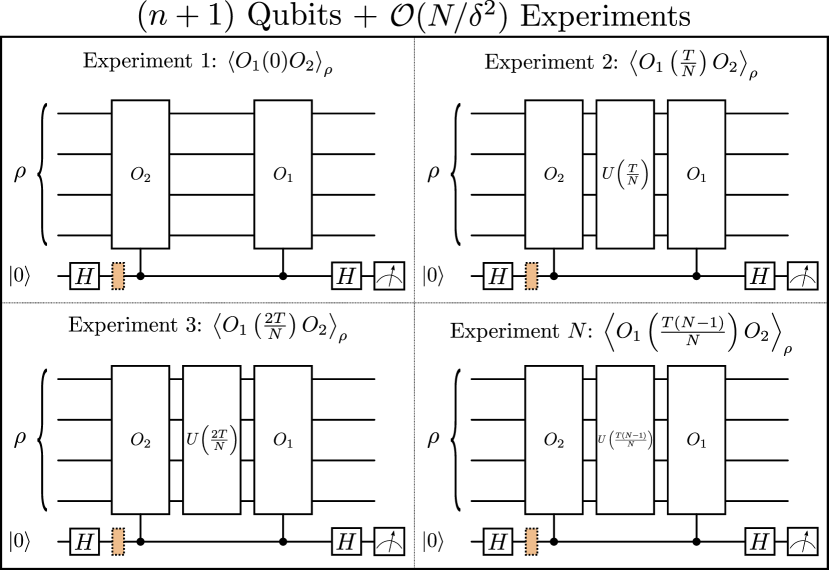
Figure 4: Algorithm for sequential-in-time estimation of Eq. (9). The algorithm show can be used to individually compute each term in the summation. That is, the circuits can be used to estimate quantities of the form $\langle O_{1}(t)O_{2}\rangle_{\rho}$. Then, one can combine those expectation values classically (as well as add the appropriate phases $e^{-i\omega\varepsilon t}$) to estimate the quantity $\widetilde{F}(O_{1},O_{2},\omega)$ up to precision $\delta$. The colored dashed gate is replaced with an identity (an $S^{\dagger}$ gate) to compute the real (imaginary) part of $\langle O_{1}(t)O_{2}\rangle_{\rho}$. This approach requires a quantum device with $(n+1)$-qubits and $\mathcal{O}(N/\delta^{2})$ different experiments.

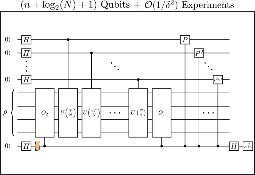
Figure 5: Algorithm for parallel-in-time estimation of Eq. (9). The algorithm shown can be used to directly estimate the quantity $\widetilde{F}(O_{1},O_{2},\omega)$ up to precision $\delta$. In the figure, $P$ denotes a $\omega\varepsilon$ phase gate. It is clear that this algorithm contains as a sub-routine the circuit for preparing the history state of Fig. 2. This approach requires a quantum device with $(n+\log(N)+1)$-qubits and $\mathcal{O}(1/\delta^{2})$ experiments. The colored dashed gate is replaced with an identity (an $S^{\dagger}$ gate) to compute the real (imaginary) part of $\widetilde{F}(O_{1},O_{2},\omega)$.

III.2 Sequential and parallel-in-time protocols

Let us now consider the task of estimating $\widetilde{F}(O_{1},O_{2},\omega)$ when $O_{1}$ and $O_{2}$ are Pauli operators by either sequential- or parallel-in-time simulations. Here, by sequential, we mean that each term in the sum in Eq. (9) is estimated on a quantum device by running some finite number of “experiment”. For instance, consider the circuit in Fig. 4, as explicitly shown in the Supplemental Information, it can be used to estimate an expectation value of the form $\langle O_{1}(\varepsilon t)O_{2}\rangle_{\rho}$. Thus, we have that the following proposition holds.

Proposition 1.

The circuit in Fig. 4, which requires $(n+1)$-qubits, can be used to estimate the quantity $\widetilde{F}(O_{1},O_{2},\omega)$ of Eq. (9) up to $\delta$ accuracy with $\mathcal{O}(N/\delta^{2})$ experiments.

The proof of Proposition 1, as well as that of all other main results, is presented in the Supplemental Information.

Clearly, the fact that we need to sequentially estimate $\langle O_{1}(\varepsilon t)O_{2}\rangle_{\rho}$ for each $t=0,\ldots,N-1$, leads to a complexity in the number of experiments (i.e., number of calls to the quantum computer) that scales as $\mathcal{O}(N)$. As we now show, this complexity can be reduced by using a scheme based on the discrete history state formalism, which allows us to directly estimate the whole sum of Eq. (9). That is, the following result holds.

Theorem 1.

The circuit in Fig. 5, which requires $(n+\log(N)+1)$-qubits, can be used to estimate the quantity $\widetilde{F}(O_{1},O_{2},\omega)$ of Eq. (9) up to $\delta$ accuracy with $\mathcal{O}(1/\delta^{2})$ experiments.

Comparing Proposition 1 and Theorem 1 reveals that by leveraging the discrete history state formalism we can trade the $\mathcal{O}(N)$ experiment-complexity for $\mathcal{O}(\log(N))$-ancillary qubits. That is, the parallel-in-time algorithm of Fig. 5 allows an exponential temporal-to-qubit resource trade-off. Here we remark that one can see from Fig. 5 that the key step behind the algorithm to compute $\widetilde{F}(O_{1},O_{2},\omega)$ is the discrete history state. In fact the circuit in Fig. 2 used to create the history state is a sub-routine in Fig. 5. Thus, by leveraging $\log(N)$ ancillas, one can simultaneously implement all $N$ time evolution operators $U(\varepsilon t)$ for $t=0,\ldots,N-1$, and concomitantly compute all the terms in the summation leading to $\widetilde{F}(O_{1},O_{2},\omega)$.

Note that while Proposition 1 and Theorem 1 are derived and proved for the case of $O_{1}$ and $O_{2}$ being unitary operators, one can readily generalize the previous results for the case when they are instead expressed as a linear combination of Pauli operators. In particular, if

$$O_{i}=\sum_{\mu=1}^{M_{1}}c^{(i)}_{\mu}U_{\mu}\,,$$ (10)

for $U_{\mu}$ being a Pauli operator, then the experiment complexities in Proposition 1 and Theorem 1 respectively change as $\mathcal{O}(NM_{1}M_{2}/\delta^{2})$ and $\mathcal{O}(M_{1}M_{2}/\delta^{2})$. Here, we again recover an exponential temporal-to-qubit resource trade-off by using the parallel-in-time algorithm.

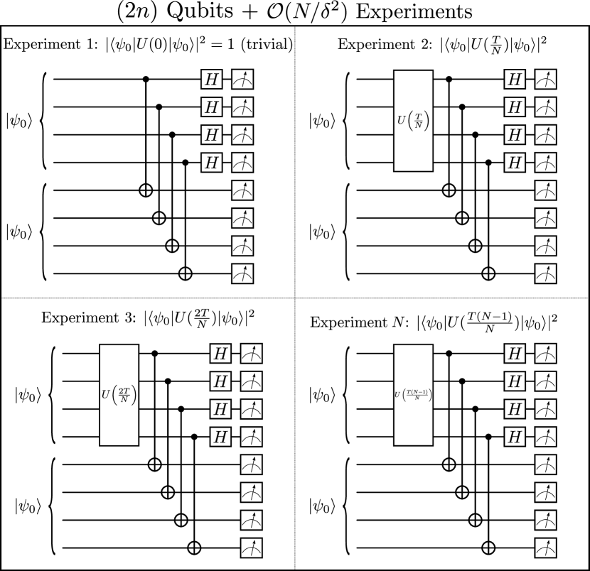
Figure 6: Algorithm for sequential-in-time estimation of the Loschmidt echo of Eq. (13). We show an algorithm which computes, up to precision $\delta$, the overlap between $\ket{\psi_{0}}$ and $U(\varepsilon t)\ket{\psi_{0}}$ for $t=0,\ldots,(N-1)$. The algorithm is based on Bell-basis measurements as described in [43]. Once these overlaps are estimating, we can average them classically to estimate discrete-time temporal average of the Loschmidt echo $\widetilde{\mathcal{L}}(\psi_{0})$. This approach requires a quantum device with $(2n)$-qubits and $\mathcal{O}(N/\delta^{2})$ different experiments.

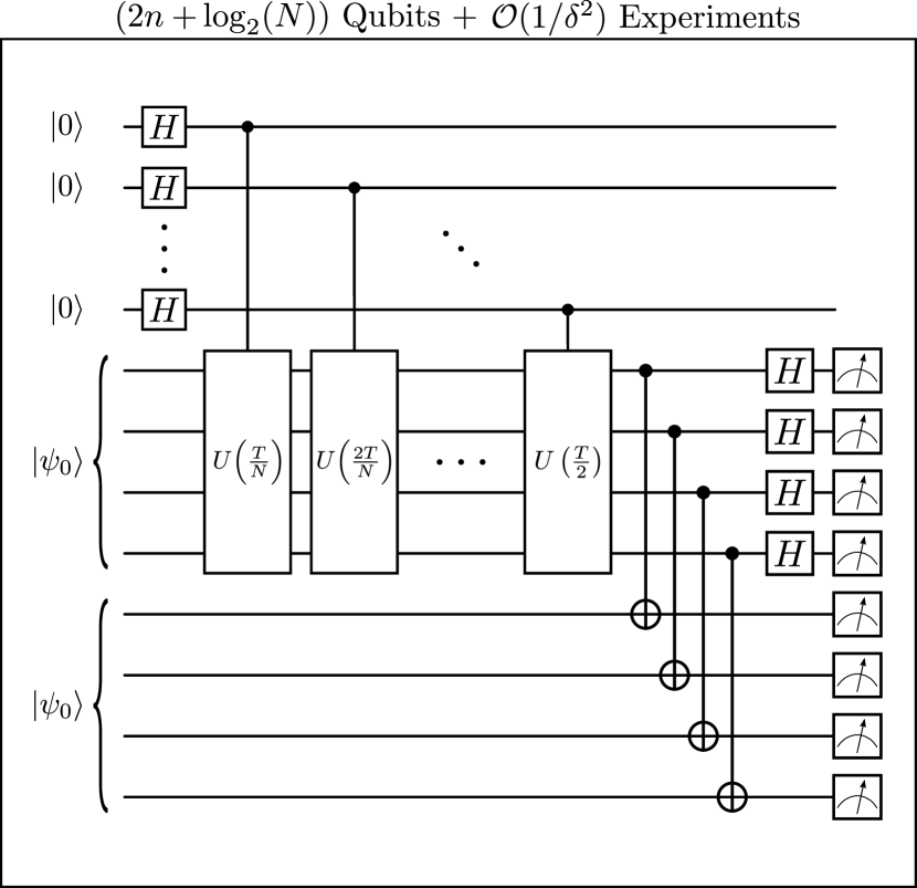
Figure 7: Algorithm for parallel-in-time estimation of the Loschmidt echo of Eq. (13). We show an algorithm which computes, up to precision $\delta$, the overlap between the discrete history state $\ket{\Psi}\!\bra{\Psi}$ and $\openone\otimes\ket{\psi_{0}}\!\bra{\psi_{0}}$. As shown in Eq. (14), the overlap between these two states is equal to $\widetilde{\mathcal{L}}(\psi_{0})$. The algorithm is based on Bell-basis measurements as described in [43]. This approach requires a quantum device with $(2n+\log(N))$–qubits and $\mathcal{O}(1/\delta^{2})$ different experiments.

Next, let us consider $\rho=O_{1}=\ket{\psi_{0}}\!\bra{\psi_{0}}$, $O_{2}=\openone$ and $\omega=0$. In this special case,

$$\overline{F}(\ket{\psi_{0}}\!\bra{\psi_{0}},\openone,0) =\lim_{T\rightarrow\infty}\int_{0}^{T}\frac{dt}{T}|\langle\psi_{0}|U(t)|\psi_{0}\rangle|^{2}\,.$$ (11)

The quantity on the right hand side is the infinite-time Loschmidt echo average  [56, 57, 59, 60], which we denote as $\bar{\mathcal{L}}(\psi_{0})$. We see that

$$\bar{\mathcal{L}}(\psi_{0})\equiv\overline{F}(\ket{\psi_{0}}\!\bra{\psi_{0}},\openone,0)\,.$$ (12)

Similarly, for its discrete-time approximation $\widetilde{\mathcal{L}}(\psi_{0})$, we can write

$$\widetilde{\mathcal{L}}(\psi_{0})\equiv\widetilde{F}(\ket{\psi_{0}}\!\bra{\psi_{0}},\openone,0)=\frac{1}{N}\sum_{t=0}^{N-1}|\langle\psi_{0}|U(\varepsilon t)|\psi_{0}\rangle|^{2}\,.$$ (13)

It is clear that while $\widetilde{\mathcal{L}}(\psi_{0})$ can technically be computed with the circuits in Figs. (4) and (5), this requires expanding $O_{1}=\ket{\psi_{0}}\!\bra{\psi_{0}}$ into a linear combination of unitaries, and such summation will generally contain exponentially many terms. To mitigate this issue, we also present two results which allow us to estimate Eq. (13) by either sequential-, or parallel-in-time simulations.

First, let us consider the following proposition.

Proposition 2.

The circuit in Fig. 6, which requires $(2n)$-qubits, can be used to estimate the quantity $\widetilde{\mathcal{L}}(\psi_{0})$ of Eq. (13) up to $\delta$ accuracy with $\mathcal{O}(N/\delta^{2})$ experiments.

Proposition (2) simply follows from applying a SWAP test [73, 74, 75, 43] (or more specifically, the state overlap algorithm of [43]) between $U(\varepsilon t)\ket{\psi_{0}}$ and $\ket{\psi_{0}}$ for $t=1,\ldots,(N-1)$. We note that the case $t=0$ is trivial as $|\bra{\psi_{0}}U(0)\ket{\psi_{0}}|^{2}=1$. When using the discrete history state we can prove the following theorem.

Theorem 2.

The circuit in Fig. 7, which requires $(2n+\log(N))$–qubits, can be used to estimate the quantity $\widetilde{\mathcal{L}}(\psi_{0})$ of Eq. (9) up to $\delta$ accuracy with $\mathcal{O}(1/\delta^{2})$ experiments.

Again, we can see from Theorem 2 that performing a parallel-in-time simulation allows us to exponentially reduce the experiment complexity (from linear in $N$ to being $N$-independent) at the cost of $\log(N)$ ancillas. Similarly to Proposition 2, the proof of Theorem 2 simply spans from computing the overlap between the discrete history state $\ket{\Psi}\!\bra{\Psi}$ and $\openone_{T}\otimes\ket{\psi_{0}}\!\bra{\psi_{0}}$. Explicitly, we have

$$\Tr[\ket{\Psi}\!\bra{\Psi}(\openone_{T}\otimes\ket{\psi_{0}}\!\bra{\psi_{0}})] =\langle\Psi|(\openone_{T}\otimes\ket{\psi_{0}}\!\bra{\psi_{0}})|\Psi\rangle$$

$$=\frac{1}{N}\sum_{t=0}^{N}\langle\psi(\varepsilon t)\ket{\psi_{0}}\!\bra{\psi_{0}}\psi(\varepsilon t)\rangle$$

$$=\widetilde{\mathcal{L}}(\psi_{0})\,.$$ (14)

IV Accessing dynamical information via system-time entanglement

Thus far, we have seen that using the history state allows us to push the complexity of running multiple experiments onto ancillary clock-qubit requirements. However, as we will now show, the entanglement present between the time and system qubits in the history state has operational meaning and contains information that we can use to learn about the system’s dynamics. Moreover, we will unveil a rigorous and explicit connection between these correlations and the equilibration problem. Protocols for obtaining these quantities from variations of the previous circuits are also provided in this section.

IV.1 Properties, relation to the problem of equilibration and to temporal fluctuations of observables

First, let us again recall that the discrete history state is a bipartite state between the system Hilbert space $\mathcal{H}_{S}$ and the time, or clock Hilbert space $\mathcal{H}_{T}$. That is, $\ket{\Psi}\in\mathcal{H}_{T}\otimes\mathcal{H}_{S}$. Moreover, it is apparent from Fig. 2 and Eq. (4) that history states are in general entangled across the system-time partition. We will henceforth refer to the correlations between the system qubits and the clock qubits as system-time entanglement (following [8]).

It is important to note that, in general, (4) is not in the Schmidt’s decomposition [76] of $|\Psi\rangle$ (as the states $\ket{\psi(t)}$ are not necessarily orthogonal). However, there exists a basis in which we can write the history state as

$$|\Psi\rangle=\sum_{l}\sqrt{p_{l}}|l\rangle_{T}|l\rangle_{S}\,,$$ (15)

where $\sqrt{p_{l}}$ are the so-called Schmidt coefficients, and $\{|l\rangle_{S}\}$, and $\{|l\rangle_{T}\}$ are orthonormal sets of states in $\mathcal{H}_{S}$ and $\mathcal{H}_{T}$, respectively. A simple way to quantify the system-time entanglement is through the linear entropy, defined as

$$E_{2}=1-\Tr[\rho_{T}^{2}]=1-\Tr[\rho_{S}^{2}]=1-\sum_{l}p_{l}^{2}\,,$$ (16)

where $\rho_{T(S)}=\Tr_{S(T)}[\ket{\Psi}\!\bra{\Psi}]$ is the reduced state of the history state in the clock (system) qubits. Here, we denote as $\Tr_{S(T)}$ the partial trace over the system (clock) qubits. In principle, one can also consider other entropies such as the Von-Neumann entropy. However, the linear entropy has the desirable property of being efficiently computable in a quantum device (see below).

There is a deep connection between the system-time entanglement and dynamical properties of the system, in particular to the problem of its equilibration: Let us recall first that given an arbitrary (for simplicity) pure state $|\psi\rangle=\sum_{k}c_{k}|k\rangle$ the infinite-time average of the associated density matrix is

$$\bar{\rho}=\int\frac{dt}{T}\sum_{k,k^{\prime}}c_{k}c_{k^{\prime}}^{\ast}e^{-i(E_{k}-E_{k^{\prime}})t}|k\rangle\langle k^{\prime}|\to\sum_{k}|c_{k}|^{2}|k\rangle\langle k|\,,$$ (17)

where one assumes large (infinite) $T$ and with $H|k\rangle=E_{k}|k\rangle$. In other words, if the state of the system is averaged over large enough times it loses all coherences in the energy basis. Under experimentally realistic conditions it is feasible to identify this state with the stationary equilibrium state [4]. For “most” observables this actually holds for short times $T$ [54], meaning that a finite time window average of observables is also an interesting quantity in general. The quantum time formalism gives a new interpretation to the loss of coherences induced by a time average: since the system is “entangled with time”, we lose information by ignoring the “clock qubits”. This loss induces precisely the (dephasing) quantum channel $\rho\to\bar{\rho}$ in the large $T$ and small $\varepsilon$ limit, a result that can be derived directly from a continuum quantum time formalism . For discrete time the following result holds.

Theorem 3.

Let $\ket{\Psi}$ be the discrete history-state in Eq. (4). The partial trace over the clock induces a quantum channel which in the large time limit implies $\rho_{S}\to\bar{\rho}$. Moreover, for any $\varepsilon$ and $N$ the following majorization relation holds:

$$\bar{\rho}\prec\rho_{S}=\tilde{\rho}\,,$$ (18)

with $\tilde{\rho}$ a discretization of Eq. (17). Furthermore, for a periodic evolution with period $\tau$ generated by a Hamiltonian with $M$ distinct eigenvalues (i.e., $e^{-iH\tau}=\openone$) and given a history state with $\log(M)$ clock qubits and time window $T=\tau$, we have

$$\rho_{S}=\bar{\rho}\,.$$ (19)

While phrased in a rather abstract way, this result has many interesting corollaries with clear operational meaning. The reason for this is that roughly speaking the history state is providing a way to prepare the equilibrated state of a quantum system: one simply needs to prepare the history state and ignore the clock-qubits. In fact, this is the reason why the previous for evaluating time averages work. Moreover, the system time entanglement entropies are in fact a lower bound to the entropies of the state in equilibrium, as it follows directly from Theorem 3 and basic majorization properties. Furthermore, one can rediscover the quantum time formalism from the natural purification of this approximate dephasing channel. The interested reader can refer to Appendix B where the proof of Theorem 3 is provided together with a more detailed discussion.

With the previous in mind, let us consider again the task of estimating the infinite-time Loschmidt echo average in Eq. (11). We recall that $\bar{\mathcal{L}}(\psi_{0})$ quantifies the degree of reversibility of the time evolution and is an indicator of the stability of the quantum system. Moreover, it is easy to see that

$$\bar{\mathcal{L}}(\psi_{0})=\Tr[\bar{\rho}^{2}]\,,$$ (20)

i.e., the infinite-time average of the Loschmidt echo is the purity of the dephased state $\bar{\rho}$. We can now use these considerations and Theorem 3 to obtain the following result.

Corollary 1.

Let $\ket{\Psi}$ be the discrete history-state in Eq. (4), and let $E_{2}$ be the linear entropy of the system-time partition. Then, for any $T$ and $N$ we have

$$E_{2}\leqslant(1-\bar{\mathcal{L}}(\psi_{0}))\,.$$ (21)

Corollary 1 has several important implications. First, it bounds the amount of entanglement between the system and the clock qubits. In particular, it shows that the system-time entanglement can only be large if the infinite-time average of the Loschmidt echo value is small. Conversely, if $\bar{\mathcal{L}}(\psi_{0})$ is large, $E_{2}$ has to be small. Second, let us remark that Eq. (21) is valid for all values of $T$, but most notably, also for all values of $N$. For large $N$ and $T$ the equality is reached asymptotically, and we have that Eq. (21) becomes $\Tr[\rho^{2}_{T}]\equiv\bar{\mathcal{L}}(\psi_{0})$. Moreover, as we will see below, our numerical analysis shows that $\Tr[\rho^{2}_{T}]$ can provide a better approximation to $\bar{\mathcal{L}}(\psi_{0})$ than $\widetilde{\mathcal{L}}(\psi_{0})$, implying that there exists no simple general relation between $E_{2}$ and $\widetilde{\mathcal{L}}(\psi_{0})$.

We can understand the intuition behind Corollary 1 as follows. Let $\ket{\psi_{0}}$ be a stationary state of the unitary evolution. For instance, let $\ket{\psi_{0}}$ be an eigenstate of $H$ with eigenenergy $E_{0}$, so that $U(\varepsilon t)\ket{\psi_{0}}=e^{-i\varepsilon tE_{0}}\ket{\psi_{0}}$. Then, the discrete history state becomes

$$\ket{\Psi}=\frac{1}{\sqrt{N}}\sum_{t=1}^{N-1}e^{-i\varepsilon tE_{0}}\ket{t}\otimes\ket{\psi_{0}}\,.$$ (22)

Equation (22) reveals that $\ket{\Psi}$ is separable. It is also not hard to verify that in this case $\widetilde{\mathcal{L}}(\psi_{0})=1$. On the other hand, if $\ket{\psi_{0}}$ evolves through $N$ orthogonal states $\bra{\psi(\varepsilon t)}\ket{\psi(\varepsilon t^{\prime})}=\delta_{tt^{\prime}}$ then Eq. (4) is already the Schmidt decomposition of $\ket{\Psi}$ and the state is maximally entangled. The previous toy model shows that if the state is quasi stationary (i.e., large Loschmidt echo), we can expect small values of entanglement. Similarly, if the state is significantly changing during the evolution (e.g., small Loschmidt echo value), then the history state will likely possess large amounts of entanglement. We note that the relation between the distinguishability of the evolved state and the system time-entanglement was first reported in [8]. However, the connection with the Loschmidt echo was not explored therein.

The result in Corollary 1 can be further strengthened for the special case where the time evolution is periodic. That is, when

$$e^{-iH\tau}=\openone\,,$$ (23)

for some $\tau$, and where we assume that $H$ has $M$ distinct eigenvalues, for $M$ being a power of two. Now, we find that the following result holds.

Corollary 2.

For a periodic evolution with period $\tau$ generated by a Hamiltonian with $M$ distinct eigenvalues, as in Eq. (23), then for a history state with $\log(M)$ clock qubits and time window $T=\tau$, we have

$$E_{2}=(1-\bar{\mathcal{L}}(\psi_{0}))=(1-\widetilde{\mathcal{L}}(\psi_{0}))\,.$$ (24)

Corollary 2 shows that for periodic Hamiltonians the system-time entanglement is exactly the same as the infinite-time average of the Loschmidt echo $\bar{\mathcal{L}}(\psi_{0})$, as well as the discrete-time approximation $\widetilde{\mathcal{L}}(\psi_{0})$. As shown in Appendix B, tracing out induces now a completely dephasing channel in the energy eigenbasis so that $\rho_{S}=\tilde{\rho}=\bar{\rho}$.

The previous results connecting the system-time entanglement with the Loschmidt echo allows us to derive even more operational meaning to $E_{2}$ as a bound for temporal fluctuations of observable. In Ref. [4], it was shown that given an observable $O$, $\bar{\mathcal{L}}(\psi_{0})$ provides a bound on temporal fluctuations of observables as

$$\sigma^{2}_{O}\leqslant\Delta_{O}^{2}\bar{\mathcal{L}}(\psi_{0})$$ (25)

with $\Delta_{A}^{2}=\lambda_{\max}[O]-\lambda_{\min}[O]$ (the difference between the largest and smallest eigenvalues of $O$ in the subspace of states satisfying $\langle n|\psi\rangle\neq 0$), and where $\sigma^{2}_{O}$ denotes the temporal variance

$$\sigma^{2}_{O}:= \overline{F(O)^{2}}-\overline{F}(O)^{2}$$ (26)

$$= \lim_{T\rightarrow\infty}\int_{0}^{T}\frac{dt}{T}\langle O(t)\rangle^{2}_{\psi_{0}}-\left(\lim_{T\rightarrow\infty}\int_{0}^{T}\frac{dt}{T}\langle O(t)\rangle_{\psi_{0}}\right)^{2}\,.$$

Here we have used the notation defined in Eq. (III.1) with $F(O)\equiv\langle O\rangle$ (at a given time) while the “overline” denotes temporal-average. Eq. (25) shows that small temporal Loschmidt echo averages imply a small temporal variance of the observable $O$, and vice versa. In other words, a system with a small $\bar{\mathcal{L}}(\psi_{0})$ can only exhibit smaller temporal fluctuations in its observables compared to a system with a large Loschmidt echo.

It should be clear to see that Theorem 1 readily implies the following corollary.

Corollary 3.

Let $O$ be an observable, and let $\sigma^{2}_{O}$ denote its temporal variance as in Eq. (26). The system-clock entanglement provides bound on temporal fluctuations as

$$\sigma^{2}_{O}\leqslant\Delta_{O}^{2}\left(1-E_{2}\right)=\Delta_{O}^{2}{\rm Tr}[\rho^{2}_{S}]\,.$$ (27)

Corollary 3 shows a clear physical meaning of the system-time entanglement. Namely, if $E_{2}$ is small, then the system is stable and predictable. This follows from the fact that the temporal variances of expectation values will be small. Conversely, if the system-time entanglement is large, then the system can be unstable and unpredictable, as evidenced by potentially large observable fluctuations.

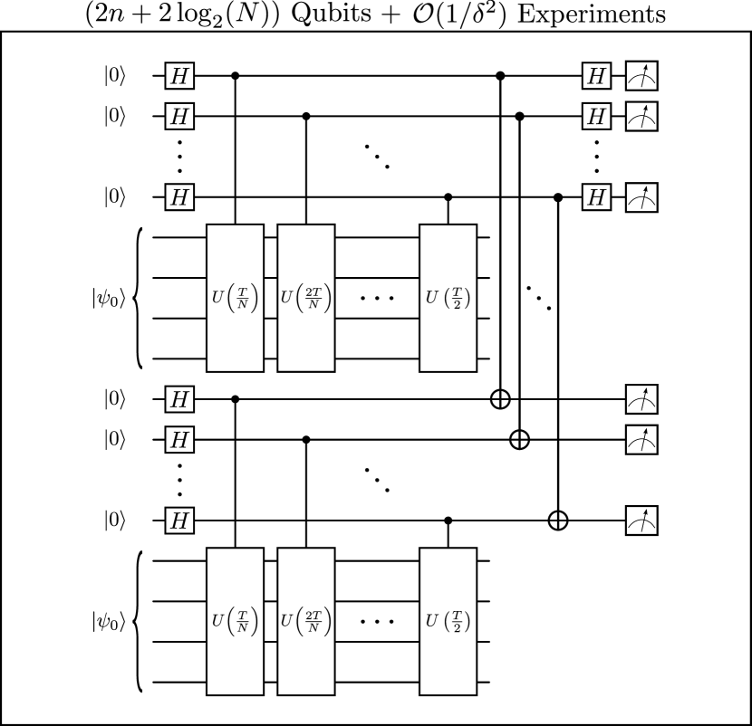
Figure 8: Algorithm for estimating $E_{2}$ via state-overlap. Here we consider the task of evaluating Eq. (16). By taking two copies of the history state, we can estimate $\Tr[\rho_{T}^{2}]$ up to $\delta$ precision via the state-overlap circuit in [43]. This approach requires a quantum device with $(2n+2\log(N))$-qubits and $\mathcal{O}(1/\delta^{2})$ different experiments.

IV.2 Protocols for computing the system-time entanglement

The previous theorems and corollary shed light on the exciting possibility of understanding the dynamics of the system through the system-time entanglement. However, in order for these results to be truly useful, one needs to be able to measure $E_{2}$ from the history state. As we can see in Eq. (16), we need to estimate $\Tr[\rho_{S}^{2}]$ or $\Tr[\rho_{T}^{2}]$. While mathematically, it makes no difference whatsoever which subsystem we focus on, as their purity is the same (see Eq. (15)), in practice it can be substantially easier to work with one system or the other.

As heuristically evidenced by our numerics (see below), the discrete history state with a number of clock qubits $\log(N)$ much smaller than the system size $n$ produces results which accurately reproduce the infinity time average properties of the system dynamics. Thus, we will henceforth assume that $\log(N)\ll n$. This assumption implies that we can compute $E_{2}$, and therefore learn about the system, by just looking at the clock qubits. We now present two methods for estimating $\Tr[\rho_{T}^{2}]$.

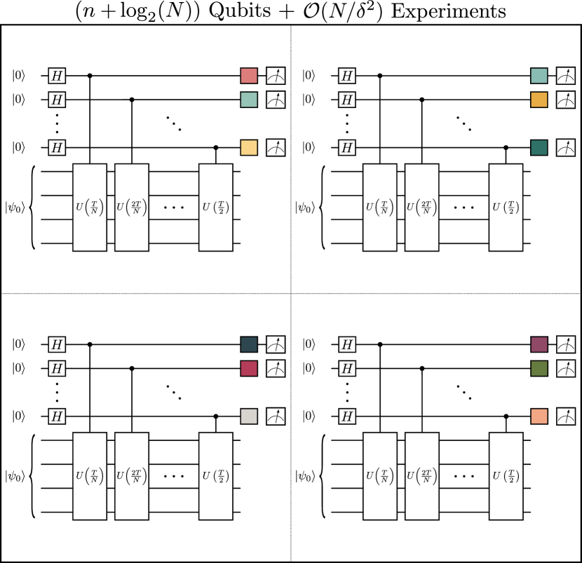
Figure 9: Algorithm for estimating $E_{2}$ via randomized measurements. Here we consider the task of evaluating Eq. (16). We start with a copy of the history state, and we apply a random unitary (indicated by a colored gate) to each qubit. Then we perform measure each qubit in the computational basis and record the measurement outcome. These constitute the so-called “classical shadows” of $\rho_{T}$. As shown in [44], this procedure allows us to estimate $\Tr[\rho_{T}^{2}]$ up to $\delta$ precision with a quantum device with $(n+\log(N))$-qubits and $\mathcal{O}(N/\delta^{2})$ different experiments.

Theorem 4.

The quantity $E_{2}$ of Eq. (16) can be estimated up to $\delta$ accuracy with the circuit in Fig. 8, which requires $(2n+2\log(N))$-qubits with $\mathcal{O}(1/\delta^{2})$ experiments. Similarly, it can also be estimated with the circuit in Fig. 9, which requires $(n+\log(N))$-qubits with $\mathcal{O}(N/\delta^{2})$ experiments.

When using the circuit in Fig. 8 one prepares two copies of the history state $\ket{\Psi}$ and then performs the state overlap circuit of Ref. [43]. On the other hand, when using the circuit in Fig. 9 one can estimate $E_{2}$ with a single copy of $\ket{\Psi}$ by using classical shadows, or randomized measurements [44, 45]. For instance, one can prepare the history state and performs a random unitary on each qubit, followed by a measurement on the computational basis. The measurement outcomes are stored and then combined classically to estimate $\Tr[\rho_{T}^{2}]$.

To finish this section, we note that by comparing Proposition 2, Theorem 2, and Theorem 4, the method to estimate either $\widetilde{\mathcal{L}}(\psi_{0})$ or $E_{2}$ with the least computational requirement (assuming $\log(N)\ll n$) is that of Fig. 9. Namely, here we can compute $E_{2}$ up to $\delta$ precision with a quantum computer with $(n+\log(N))<<2n$ qubits and with $\mathcal{O}(N/\delta)$ experiments. This result then showcases the power of using the history state as it allows us to study physical properties of the system (such as bounding $\bar{\mathcal{L}}(\psi_{0})$ or the temporal variances $\Delta O^{2}$) with less requirements than we would otherwise need.

V Depth-Estimation and parallel-in-time advantages

In the previous sections we have presented several methods where we used the history state to study temporal averages of quantities of the form of $\widetilde{F}(O_{1},O_{2},\omega)$ in Eq. (9). At the same time, we have shown how to compute the system-time entanglement, a new quantity with many interesting applications. Crucially, these techniques require being able to implement the phase estimation-like circuit for preparing history states in Fig. 2 as a sub-routine. In this section, we give an explicit estimation of the depth of this preparation circuit based on two different implementations: a direct Lie-Trotter product formula [78] approach and a Hamiltonian diagonalization scheme which we implemented variationally  [46]. The aim is to compare the associated running times of the algorithms with the ones obtained in sequential methods, focusing only on the parts of the protocols involving evolution gates.

V.1 Direct Trotterization approach

We start by recalling that $U(\varepsilon t)=e^{-iH\varepsilon t}$ for some Hamiltonian of interest $H$. Usually, if one wishes to implement $U(\varepsilon t)$, the standard approach is to break the evolution into a smaller, easier to implement evolutions $U(\varepsilon)$, and then repeat it $t$ times. That is, one has $U(\varepsilon t)=U(\varepsilon)^{t}$. In this way, the depth of the circuit needed to implement $U(\varepsilon t)$ grows with $t$.

To be more specific, let us assume that one is employing a Lie-Trotter decomposition-based product formula. This was the first example of quantum advantage for quantum simulations [78] and remains a relevant and straightforward technique to this day [79]. The basic idea is to decompose a given Hamiltonian $H=\sum_{j=1}^{l}h_{j}$ as $U(\varepsilon)\approx\prod_{j}e^{-ih_{j}\varepsilon}$. We will further assume that each $h_{j}$ is local, i.e., it acts non-trivially on at most $\mathcal{O}(1)$ qubits. Importantly, note that the locality condition implies that $l$ is at most polynomially growing with the system size. The evolution operator up to time $\tau=t\varepsilon$ can be approximated with $t$ copies of these gates as $U(\tau)\approx\Big{[}\prod_{j}e^{-ih_{j}\varepsilon}\Big{]}^{t}$ which is also logarithmic in the system size.

A rough estimation of the error involved was provided in [78] by assuming that the main contribution to the error comes from the second-order term in the Lie-Trotter formula. Under this assumption, the number of times steps required for guaranteeing a fixed precision grows as $t\propto\tau^{2}$. Then, the total number of gates, denoted as $\#_{g}(\tau)$, scales as $\#_{g}(\tau)=\gamma l\tau^{2}$ for $\gamma$ a constant dependent on the precision and the particular Hamiltonian. More general bounds were found in [80] which allows us to write $\#_{g}(\tau)=\gamma l\tau^{\alpha}$. This is the estimation we will be using. Under certain scenarios, this bound can be improved e.g. by using the Lie-algebraic structure associated with the given Hamiltonian [81], and in general, the “actual” error scaling of such product formulas remains poorly understood [79]. For our purpose the previous bound will suffice: we want to compare the total number of gates required in the sequential (Figures 4 and 6) versus the parallel-in-time approach (Figures 5 and 7) assuming the same Trotterization scheme is applied to both. The interest in this quantity relies on the fact that the total number of gates employed in each simulation protocol is what determines the total time span required to complete the computation . By estimating this quantity in each protocol we can establish whether it is more convenient to use a sequential or parallel-in-time approach.

Theorem 5.

Consider the total number of gates required for implementing the evolution in the sequential approaches $\#^{\text{seq}}$, and the total number for the parallel in time approaches $\#^{\text{par}}$. They scale as $\#^{\text{seq}}\in\mathcal{O}(lN^{\alpha+1})$, $\#^{\text{par}}\in\mathcal{O}(l^{2}N^{\alpha})$ yielding

$$\#^{\text{par}}\sim\frac{\beta l}{N}\#^{\text{seq}}\,,$$ (28)

for $\beta\in\mathcal{O}(1)$ a constant independent both of the system and clock size.

Theorem 5 is a consequence of the fact that $\#^{\text{seq}}$ is given by the sum over the amount of gates of each run so that $\#^{\text{seq}}\sim N^{\alpha+1}$. Instead, in the parallel approach the total number gates only involves a sum over the $log(N)$ gates of the same run, thus giving $\#^{\text{seq}}\sim N^{\alpha}\beta l$. The extra factor $\beta l$ comes from the fact that those gates need to be controlled. Remarkably, the depth scaling with the number of times of the parallel-in-time approach is the same as the one of a single Trotter evolution up to time $\tau\equiv\varepsilon N$. See Appendix D for the details and the proof of the previous theorem.

Something really interesting has happened: in the parallel approach we have an increase in depth which is logarithmic in the system size, but we have reduced the total number of gates exponentially in the number of clock qubits (with respect to a sequential approach). We can then state the following:

Proposition 3.

Given $\log(N)$ clock-qubits and system of dimension $d$, the parallel-in-time approach outperform the computational times of the sequential approach for

$$\log(N)\gtrsim\log(\beta l)\sim\log(\beta\log(d))\,.$$ (29)

Remarkably, the condition for a convenient clock size is doubly logarithmic in the system’s Hilbert space dimension $d$. Typically, a modest number of qubits for the clock, much smaller than the system size, is sufficient to improve computational times.

Finally, let us remark that Proposition 3 will hold under rather general conditions, since it is based on the fact that a sum over $N$ terms is involved in the estimation of $\#^{\text{seq}}$, while a sum over $\log(N)$ terms is required for $\#^{\text{par}}$ (see proof in Appendix F). However, the scaling of the number of gates $\#^{\text{par}}$ we provided in Theorem 5 is still based on a pessimistic bound and linked to product formulae: the generic bounds we used for Trotterization can overestimate by far [83, 84] the actual errors, which depend on the specific initial states and observables involved in the complete protocols. This means that actual implementations of the parallel-in-time protocols, whether based on product formulae or more advanced methods, might be much more efficient. The important message is that the advantages over sequential-in-time protocols, as stated in Proposition 3, hold more generally (see also below).

V.2 Hamiltonian diagonalization and Cartan decomposition approach

In this section, we repeat the circuit depth analysis in another relevant scheme, namely assuming one has access to a diagonalization of the Hamiltonian. In particular, we will also discuss how one can obtain such diagonalization variationally via the algorithm presented in [46].

Let us recall that there always exists a unitary $W$ (whose columns are the eigenvectors of $H$) and a diagonal matrix $D$ (whose entries are the eigenvalues of $H$) such that

$$H=WDW^{\dagger}\,.$$ (30)

Without loss of generality, we can expand $D$ is some basis of mutually commuting operators

$$D=\sum_{\mu}c_{\mu}h_{\mu}\,,$$ (31)

where $[h_{\mu},h_{\mu^{\prime}}]=0$ for all $\mu,\mu^{\prime}$. If one has access to $W$ and $D$, then the unitary evolution can be expressed as

$$U(\varepsilon t) =U(\varepsilon)^{t}$$

$$=We^{-iD\varepsilon t}W^{\dagger}$$

$$=We^{-i\sum_{\mu}c_{\mu}\varepsilon th_{\mu}}W^{\dagger}$$

$$=W\left(\prod_{\mu}e^{-ic_{\mu}\varepsilon th_{\mu}}\right)W^{\dagger}\,,$$ (32)

The power of Eq. (32) can be seen from Fig.  10, where it is shown that we can use the diagonalization of $H$ to implement $U(\varepsilon t)$ at fixed depth. Namely, the circuit depth for $\prod_{\mu}e^{-ic_{\mu}\varepsilon th_{\mu}}$ and for $\prod_{\mu}e^{-ic_{\mu}\varepsilon th_{\mu}t^{\prime}}$ is exactly the same, we just change the parameters associated to each time evolution generated by $h_{\mu}$. This means that in a sequential approach, each run requires $\mathcal{O}(n)$ gates independently of the evolution time, and assuming for simplicity that each $h_{\mu}$ acts as a one-body operator. The total number of gates is then $\#^{\text{seq}}=\mathcal{O}(nN)$.

Moreover, the benefits of diagonalizing the Hamiltonian $H$ are amplified when using this technique in the circuit for preparing the history state. As shown in Fig. 11(a), we can see that instead of controlling $\log{N}$ gates $U(2^{j-1}\varepsilon)$ (where for $j=1,\ldots,\log{N}$), the history state can be prepared by first acting on the system qubits with the non-controlled unitary $W$, followed by $\log{N}$ controlled gates $e^{-iD2^{j-1}\varepsilon}$, and finally by implementing a non-controlled unitary $W^{\dagger}$. This further reduces the depth required to prepare the history state. First, we do not need to control $W$, nor $W^{\dagger}$. Second, we note that controlling $e^{-iD\varepsilon t}$ (for any $t$) is equivalent to controlling each term $e^{-ic_{\mu}\varepsilon th_{\mu}}$ (since the $h_{\mu}$ are mutually commuting). For instance, we can see in Fig. 11(b) that if the $h_{\mu}$ are single-qubit Pauli operators acting on each qubit, then implementing a controlled $e^{-iD\varepsilon t}$ gate, just requires controlling $n$ single qubit rotations. This gives the following Theorem.

Theorem 6.

By replacing the history state preparation subroutine with the diagonalized Hamiltonian as in Eq. (30) and Fig. 11, we can prepare the history state with a total number of gates

$$\#^{\text{par}}\in\mathcal{O}(\log(N)n)$$ (33)

i.e. logarithmic in both the number of times and system size.

The parallel-in-time advantage over the sequential approach condition now becomes $N>\beta\log(N)$, which is independent of the system size and is virtually always reached. Of course, one could argue that if we have classical access to the diagonalized Hamiltonian, then we could just expand the initial state state and the measured operators in the energy eigenbasis to compute any expectation value. However, this kind of expansion will not be tractable for large problem sizes. Instead, we will show below that if $W$ is accessible in a quantum computer, then one can still leverage the diagonalization for depth reduction.

Finally, we note that if we want to study the entanglement in $\rho_{T}$ as in Theorems 1 and 4 (see also Figs. 8 and 9), then the final unitary $W^{\dagger}$ in Fig. 11(a) can be omitted. This is due to the fact that the entanglement is invariant under local unitaries [85], and hence $W^{\dagger}$ cannot change the entanglement nor the spectral properties of $\rho_{T}$.

Figure 10: Depth-reduction via Hamiltonian diagonalization. On the left, we implement $U(\varepsilon t)$ by expanding the evolution into shorter-time evolutions $U(\varepsilon)$ (which we can then implement via Trotterization), and then perform $U(\varepsilon t)=U(\varepsilon)^{t}$. This comes at the cost of increasing the depth as $t$ is increased. On the right, we use the diagonalization of $H$ as in Eq. (30) to express $U(\varepsilon t)=We^{-iD\varepsilon t}W^{\dagger}$. Moreover, it can be seen by expanding $D$ in a basis of mutually commuting operators (as in Eq. (31)) that the circuit implementation of $e^{-iD\varepsilon t}$ has the same depth for any $t$ (see also Eq. (32)).

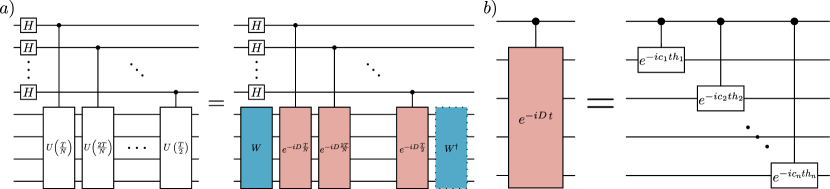
Figure 11: History state via Hamiltonian diagonalization. a) Here we show how the circuit in Fig. 2 for preparing the history state changes when using the Hamiltonian diagonalization. In particular, we see that instead of controlling the $\log{N}$ gates $U(2^{j-1}\varepsilon)$ for $j=1,\ldots,\log{N}$ we now need to implement non-controlled unitaries $W$ and $W^{\dagger}$, and simply control the fixed-depth $\log{N}$ gates $e^{-iD2^{j-1}\varepsilon}$ for $j=1,\ldots,\log{N}$. We note that if we only care about the entanglement in $\rho_{T}$ as in Figs. 8 and 9, then the final unitary $W^{\dagger}$ can be omitted (the entanglement is invariant under local unitaries [85]). b) For the special case when the diagonal Hamiltonian $D$ is expressed as a sum of single-qubit operators acting on each qubits (i.e., $h_{\mu}$ in Eq. (31) is a one-body operator acting on the $\mu$-th qubits), then controlling the gates $e^{-iD2^{j-1}\varepsilon}$ simply requires controlling single-qubit gates.

It is worth highlighting the fact that the main challenge for using Eq. (32) is that it requires access to the decomposition in Eq. (30), and that $W$ and $D$ might not be readily accessible. However, one can still attempt to variationally learn them [48]. For example, one can use the Variational Hamiltonian Diagonalization algorithm in Ref. [46] which is aimed at training a parametrized ansatz for the diagonalization of $H$. The ansatz is composed of two parts: 1) A parametrized unitary $W(\bm{\alpha})$, and 2) A diagonal Hamiltonian $D(\bm{\beta})$ such that

$$\widehat{H}(\bm{\alpha},\bm{\beta})=W(\bm{\alpha})D(\bm{\beta})W^{\dagger}(\bm{\alpha})\,.$$ (34)

One can quantify how much $\widehat{H}(\bm{\alpha},\bm{\beta})$ approximates the target Hamiltonian $H$ by defining the cost function

$$C(\bm{\alpha},\bm{\beta})=\frac{\norm{H-\widehat{H}(\bm{\alpha},\bm{\beta})}_{HS}^{2}}{2^{n}}\,,$$ (35)

where $\norm{X}_{HS}=\sqrt{\Tr[X^{\dagger}X]}$ is the Hilbert-Schmidt norm. Clearly, the cost is equal to zero if $H=\widehat{H}(\bm{\alpha},\bm{\beta})$. Thus, the parameters $\bm{\beta}$ and $\bm{\alpha}$ are trained by solving the optimization task

$$\operatorname*{arg\,min}_{\bm{\beta},\bm{\alpha}}C(\bm{\alpha},\bm{\beta})\,.$$ (36)

Here, where a quantum computer is used to estimate the term in $C(\bm{\alpha},\bm{\beta})$ [46], while classical optimizers are used to train the parameters.

In this variational setting, it is extremely important to pick an ansatz (i.e., a given unitary $W(\bm{\alpha})$, and diagonal Hamiltonian $D(\bm{\beta})$) which do not lead to trainability issues such as barren plateaus [86, 87, 88, 52], where the cost function gradients are exponentially suppressed with the problem size. One of the leading strategies to mitigate such issues is to use the so-called problem-inspired ansatzes, where one creates ansatzes with strong inductive biases [89, 90, 91] based on the problem at hand. Recently, one such method was developed which is exploits the Cartan decomposition of the Lie algebra generated by the target Hamiltonian $H$ [92, 93, 94]. Below we explain such method.

Consider the Hamiltonian of interest $H$. Then, without loss of generality we assume that it can be expressed as a sum of Hermitian traceless operators $\{H_{i}\}$ as

$$H=\sum_{i}a_{i}H_{i}\,,$$ (37)

where $a_{i}\in\mathbb{R}$. Then, let $\mathfrak{g}=\langle\{iH_{i}\}\rangle_{Lie}$ be the Lie closure of the set of operators [95]. Note that, by definition, $iH\in\mathfrak{g}$. The result in Ref. [47], provides an efficient-in-$\dim(\mathfrak{g})$ circuit for the simulation of any $e^{-iHt}$ for any set of coefficients $\{a_{i}\}$. To understand the technique of Ref. [47], we recall that a Cartan decomposition of the Lie algebra $\mathfrak{g}$ refers to the decomposition of $\mathfrak{g}$ into two orthogonal subspaces $\mathfrak{g}=\mathfrak{k}\oplus\mathfrak{m}$, where $\mathfrak{k}$ is a Lie subalgebra, i.e., $[\mathfrak{k},\mathfrak{k}]\subseteq\mathfrak{k}$, whereas $\mathfrak{m}$ is not: $[\mathfrak{m},\mathfrak{m}]\subseteq\mathfrak{k}$. Moreover, these two orthogonal subspaces satisfy $[\mathfrak{k},\mathfrak{m}]=\mathfrak{m}$, and $\mathfrak{m}$ contains the maximal commutative subalgebra, also known as the Cartan subalgebra, $\mathfrak{h}$ of $\mathfrak{g}$. Note that for any pair of element $ih_{1}$ and $ih_{2}$ in $\mathfrak{h}$, we have $[h_{1},h_{2}]=0$.

The Cartan decomposition provides us an ansatz to diagonalize $H$ as follows. First we note that $H$ always admits a decomposition of the form

$$H=WhK^{\dagger}\,,$$ (38)

with $K\in e^{\mathfrak{k}}$ and $h\in\mathfrak{h}$. Reference [47] provides us with an ansatz for Eq. (34) as we can now parametrize and optimize over the Lie group $e^{\mathfrak{k}}$ and the algebra $\mathfrak{h}$. That is, we simply pick

$$W(\bm{\alpha})=\prod_{\nu}e^{i\alpha_{\nu}B_{\nu}}\,,$$ (39)

where $iB_{\nu}$ belongs to a basis of $\mathfrak{k}$, and

$$D(\bm{\beta})=\sum_{\mu}\beta_{\mu}h_{\mu}\,,$$ (40)

with $ih_{\mu}$ belonging to a basis of $\mathfrak{h}$. Taken together, Eq. (39) and (40) provide a problem-inspired ansatz for the diagonalization of $H$ which we can use to solve Eq. (36).

V.2.1 Example: $XY$ model.

Let us here exemplify the Cartan decomposition-based method. Consider a general $XY$ Hamiltonian of the form

$$H=\sum_{j=1}^{n-1}a_{j}^{x}X_{j}X_{j+1}+a_{j}^{y}Y_{j}Y_{j+1}+\sum_{j}a_{j}^{z}Z_{j}\,;$$ (41)

Here, one can prove that $\mathfrak{g}=\langle i\{X_{j}X_{j+1},Y_{j}Y_{j+1},Z_{j}\}\rangle_{\text{Lie}}\cong\mathfrak{so}(2n)$. Thus, the ensuing Cartan decomposition is

$$\mathfrak{k}= {\rm span}\{\widehat{X_{i}Y_{j}},\widehat{Y_{i}X_{j}}\,|\,1\leqslant i<j\leqslant n\}\cong\mathfrak{so}(n)\oplus\mathfrak{so}(n)$$ (42)

$$\mathfrak{m}= {\rm span}\{Z_{j},\widehat{X_{i}X_{j}},\widehat{Y_{i}Y_{j}}\,|\,1\leqslant i<j\leqslant n\}$$ (43)

$$\mathfrak{h}= {\rm span}\{Z_{j}\,|\,1\leqslant i\leqslant n\}\cong\oplus_{i=1}^{n}\mathfrak{u}(1)$$ (44)

where we used the notation $\widehat{A_{i}B_{j}}=A_{i}Z_{i+1}\cdots Z_{j-1}B_{j}$.

Here, we can see that the ansatz for the diagonal part of the ansatz in Eq. (34) is simply

$$D(\bm{\beta})=\sum_{j=1}^{n}\beta_{\mu}Z_{j}\,.$$ (45)

On the other hand, it is clear from Eqs. (39) and (42) that a drawback in the proposal of Ref. [47] is that it requires us to implement gates which are obtained by exponentiation of highly non-local operators (e.g. $e^{-i\alpha\widehat{X_{1}Y_{n}}}$), a task which can be hard to implement and lead to deep circuits. Hence, we propose a different parametrization for $W(\bm{\alpha})$. Consider the following set of local operators.

$$\mathcal{G}=\{X_{j}Y_{j+1},Y_{j}X_{j+1}\}_{j=1}^{n-1}\subset\mathfrak{k}\,.$$ (46)

We can prove that the following proposition holds.

Proposition 4.

$i\mathcal{G}$ is a generating set of the algebra $\mathfrak{k}$. That is, $\langle i\mathcal{G}\rangle_{Lie}=\mathfrak{k}$ .

The key implication of Proposition 4 is that we can generate any unitary in the unitary subgroup $e^{\mathfrak{k}}$ by exponentiating only the local operators in $\mathcal{G}$. This means, that one can diagonalize $H$ using an ansatz of the form

$$W(\bm{\alpha})=\prod_{l=1}^{L}\prod_{j=1}^{n-1}e^{i\alpha_{j,l}X_{i}Y_{i+1}}\prod_{j=1}^{n-1}e^{i\alpha_{j,l}Y_{i}X_{i+1}}\,.$$ (47)

We explicitly show the form of this ansatz in Fig. 12. Note that since the operators in Eq. (47) are two-body, then the circuit for $W(\bm{\alpha})$ only requires local two-qubit gates. Hence, such construction significantly reduces the circuit requirements over that in Ref. [47].

The question still remains to how large $L$ needs to be. Here, we can leverage recent results from the quantum machine learning literature which state that by taking $L\geqslant\dim(\mathfrak{k})/(2n-2)$ it is generally sufficient to guarantee that any $K\in e^{i\mathfrak{k}}$ will be expressible [90]. Moreover, in this regime the ansatz is said to be overparametrized. In this overparametrization regime, the optimization of Eq. (36) becomes much easier to solve as many spurious local minima disappear [90, 96].

Putting the previous results together, and assuming we can efficiently solve Eq. (36), we can derive the following theorem.

Theorem 7.

Let $H$ be an $XY$ Hamiltonian of the form in Eq. (41). Then, let $D(\bm{\beta})$ be a diagonal operator as in Eq. (45), and let $W(\bm{\alpha})$ be a unitary as in (47). By replacing the history state preparation subroutine with the trained diagonalized Hamiltonian as in Eq. (34) and Fig. 11, we can implement the circuits used in Theorems 1, 2, and 4 with circuit depths in $\mathcal{O}(\log(N)n)$.

The results in Theorem 7 showcase the extreme power of diagonalizing $H$ via its Cartan decomposition as we can implement all the circuits in Figs. 5, 7, 8, and 9 with a depth that only scales as the product of the number of system and clock qubits.

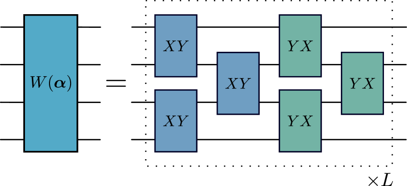
Figure 12: Ansatz for $W(\bm{\alpha})$. By using Proposition 4 we propose an ansatz for the diagonalizing unitary $W(\bm{\alpha})$ which only uses local gates acting on neighbouring qubits. We shown here a single “layer” of an $n=4$ ansatz which is repeated $L$ times.

VI Numerical simulations

In this section we first provide numerical simulations that showcase how the discrete-time approximations (computable via our algorithms) can capture the behaviour of their continuum time counterparts. Similarly, we also show numerically that the system-time entanglement provides a new way to understand dynamical properties of the system. Next, we will demonstrate how the variational Hamiltonian diagonalization algorithms can be used to reduce the depth of the history state preparation circuit, as discussed in Section V.2.1.

Figure 13: Average approximation error $|\bar{\mathcal{L}}(\psi_{0})-\widetilde{\mathcal{L}}(\psi_{0})|$ for a chain of $n=200$ sites. The vertical indicates the number of clock qubits while the horizontal axis is the window size $\varepsilon$. The blue (solid) curves represent constant values of $T$ with the arrows pointing toward the direction of greater resolution. Green arrows indicate a cross cut of fixed $\varepsilon$ an increasing $\log(N)$ that is shown in further detail in Fig. 14.

In all of our experiments, we consider a system of $n$-qubits evolving by a unitary generate by the time-independent non-uniform $XX$ model, whose Hamiltonian reads

$$H=\frac{J}{4}\sum_{j=1}^{n}(X_{j}X_{j+1}+Y_{j}Y_{j+1})+\frac{\lambda}{4}\sum_{j=1}^{n}\cos(2\pi\alpha j)(Z_{j}+2)\,,$$ (48)

where we define periodic boundary conditions as $h_{n+1}\equiv h_{1}$ (for $h=X,Y,Z$). For $\alpha=\frac{\sqrt{5}-1}{2}$, one can use the Jordan-Wigner transformation [97] (see details in Appendix G) to show that in the thermodynamic limit this model exhibits a delocalization-localization transition at the critical point $\lambda=J$. Indeed, it is well known that such transition induces sharp changes in long-time dynamical properties such as the Loschmidt echo average [60]. Our goal is then use this paradigmatic model as a test-bed to show that our proposed discrete-time average of the Loschmidt echo can capture the behavior of their continuum time counterparts.

VI.1 Discrete time averages and system-time entanglement

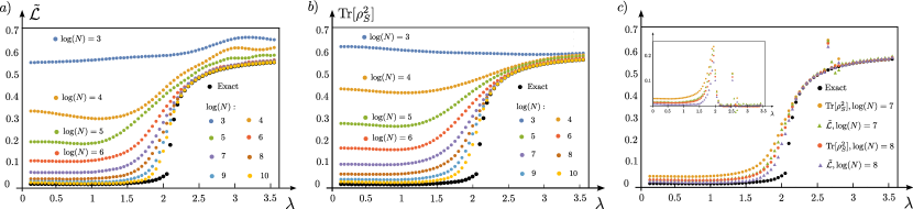
Figure 14: Discrete-time approximations to the Loschmidt echo $\bar{\mathcal{L}}(\psi_{0})$ (black dots) as a function of $\lambda$ for a chain of $n=200$ sites.. In panel $a)$ we depict the exact infinite-time average , as well as the discrete-time approximation $\widetilde{\mathcal{L}}(\psi_{0})$ for different values of clock qubits $\log(N)$ and for $\varepsilon=0.45$. In $b)$ we depict the exact infinite-time average $\bar{\mathcal{L}}(\psi_{0})$ (black dots), as well as the purity of the reduced state $\rho_{S}=\Tr_{T}[\ket{\Psi}\!\bra{\Psi}]$ for different values of clock qubits $\log(N)$ and for $\varepsilon=0.45$. In $c)$ we depict the exact infinite-time average $\bar{\mathcal{L}}(\psi_{0})$ (black dots), its discrete-time approximation $\widetilde{\mathcal{L}}(\psi_{0})$, as well as the purity of the reduced state $\rho_{S}=\Tr_{T}[\ket{\Psi}\!\bra{\Psi}]$ for different values of clock qubits $\log(N)$and for $\varepsilon=1.25$. The inset corresponds to the difference between each approximation and $\bar{\mathcal{L}}(\psi_{0})$.

To study the discrete-time average of the Loschmidt’s echo we have considered a chain of $n=200$ sites with $J=2$, $\alpha=\frac{\sqrt{5}-1}{2}$, and a number of clock qubits ranging from $1$ to $10$, corresponding to a maximum number of $N=1024$ times. Note that with this choice, the system dimension is equal to $2^{200}$ and hence, much larger than the clock Hilbert space dimension, $N$. To study the effects of the window size, we have also considered values of $\varepsilon$ spanning from $0.05$ up to $1.95$ with spacing $0.1$ (see Fig. 3). The initial state of our simulations is $|\psi_{0}\rangle=(s^{+}_{99}+s^{+}_{100}+s^{+}_{101})|\downarrow\downarrow\dots\downarrow\rangle/\sqrt{3}$, where $s^{+}_{j}$ denotes the creation operator at site $j$. As such, at $t=0$, the state is only partially delocalized in the middle of the chain. All simulations, including the computation of the exact infinite-time average $\bar{\mathcal{L}}(\psi_{0})$, where performed via Jordan-Wigner diagonalization, and we refer the reader to Appendix G for additional details.

In Fig. 13 we first present a two-dimensional plot of the error between the infinite-time average of the Loschmidt echo $\bar{\mathcal{L}}(\psi_{0})$ and its discrete-time approximation $\widetilde{\mathcal{L}}(\psi_{0})$ ($|\bar{\mathcal{L}}(\psi_{0})-\widetilde{\mathcal{L}}(\psi_{0})|$) averaged over $\lambda\in(0.1,3.5)$ (with spacing $\Delta\lambda=0.05$), for different values of $\varepsilon$ and $n$. Here, we can see that, as expected, the error is reduced by increasing the number of clock qubits. The improvement follows two tendencies. First, there is an overall improvement when increasing $T$ (i.e., when moving up in the $\log(N)$ axis for fixed $\varepsilon$), as this corresponds to better accuracy. On the other hand, for constant $T$ it is beneficial to reduce $\varepsilon$ (i.e., increase resolution), as shown by the blue solid curves.

We further explore the effect of fixing $\varepsilon$ and increasing $\log(N)$ in Fig. 14 $a)$. Therein we show $\bar{\mathcal{L}}(\psi_{0})$, as well as its discrete-time approximation $\widetilde{\mathcal{L}}(\psi_{0})$ for different number of clock qubits as a function of $\lambda$ for fixed resolution $\varepsilon=0.45$ (vertical dashed line in Fig. 13). First, we note that the infinite-time Loschmidt echo captures the delocalization-localization transition occurring at $\lambda=J=2$. In particular, for $\lambda<2$ we see that $\bar{\mathcal{L}}(\psi_{0})$ is small, indicating a delocalized phase. On the other hand, for $\lambda>2$ the evolved state is localized as $\bar{\mathcal{L}}(\psi_{0})$ is large. Next, let us note that as $\log(N)$ increases, $\widetilde{\mathcal{L}}(\psi_{0})$ quickly becomes a good approximation for its infinite-time counterpart (as expected from Fig. 13). However, Fig. 14 also reveals that $\widetilde{\mathcal{L}}(\psi_{0})$ capture the delocalization-localization transition even for a small number of clock qubits. Already for $\log(N)=6$ the inflection point of $\widetilde{\mathcal{L}}(\psi_{0})$ approaches the critical value $\lambda=2$.

Next, we study how the system-time entanglement, as measured through the subsystem purity $\Tr[\rho_{S}^{2}]$ for $\rho_{S}=\Tr_{T}[\ket{\Psi}\!\bra{\Psi}]$, approximates the infinite-time average Loschmidt echo (see Corollary 1). In Fig. 14 $b)$ we plot $\bar{\mathcal{L}}(\psi_{0})$, as well as $\Tr[\rho_{S}^{2}]$, for different number of clock qubits as a function of $\lambda$. Again, we see a clear convergence towards $\bar{\mathcal{L}}(\psi_{0})$ as the number of clock qubits are increased. This result shows that the subsystem purity provides an excellent approximation of $\bar{\mathcal{L}}(\psi_{0})$. Moreover, one can also observe that the system-time entanglement clearly captures the delocalization-localization transition. This fact can be readily understood from the fact that in the localized phase the state does not change considerably with time, and hence a small amount of entanglement is expected. This example perfectly exemplifies the fact that the system-time entanglement in the history state carries valuable information about the system dynamics. Moreover, since we know that $\Tr[\rho_{S}^{2}]=\Tr[\rho_{T}^{2}]$, then one can estimate the reduced state tomography by studying only the reduced state on the $\log(N)(\ll n)$ clock qubits.

Figures 14 $a)$ and $b)$ show that both the discrete-time Loschmidt echo and the subsystem purity provide good approximations of $\bar{\mathcal{L}}(\psi_{0})$. To better compare their performance, we show in Fig. 14 $c)$ curves for $\bar{\mathcal{L}}(\psi_{0})$, $\widetilde{\mathcal{L}}(\psi_{0})$ and $\Tr[\rho_{S}^{2}]$ for the same chain of $n=200$ spins, but for $\varepsilon=1.25$, i.e., for less accuracy (see Fig. 3). In this regime, one can see that while $\widetilde{\mathcal{L}}(\psi_{0})$ suffers from undesired oscillations, $\Tr[\rho_{S}^{2}]$ can still provide a good approximation for the same number of qubits. In particular, Fig. 14 $c)$ shows that $\widetilde{\mathcal{L}}(\psi_{0})$ can be smaller than $\bar{\mathcal{L}}(\psi_{0})$ in unpredictable ways (due to insufficient resolution), meaning that $\widetilde{\mathcal{L}}$ cannot be strictly used to provide strict bounds such as the one in Corollary 1. While ${\rm Tr}[\rho_{S}^{2}]$ oscillates as well, this quantity never crosses the black points, in agreement with our bounds. Here we also observe that the system-time entanglement provides a better convergence in the localized region. On the other hand, the entanglement curves are above the $\widetilde{\mathcal{L}}$ curves in the delocalized sector. Notice however that this discrepancy can be mitigated by increasing the number of qubits. Finally, we note that in Fig. 14 $c)$ we also depict the differences $\left(\widetilde{\mathcal{L}}(\psi_{0})-\bar{\mathcal{L}}(\psi_{0})\right)$ and $\left(\Tr[\rho_{S}^{2}]-\bar{\mathcal{L}}(\psi_{0})\right)$, which confirm that $\Tr[\rho_{S}^{2}]$ is always strictly larger than $\bar{\mathcal{L}}(\psi_{0})$, whereas $\widetilde{\mathcal{L}}(\psi_{0})$ can indeed be smaller that the infinite-time average.

Finally, as an example of Corollary 3 we also numerically show how the system-time entanglement provides a bound for the fluctuation of observables. We use as an example the observable $O=s^{+}_{L/2}s^{-}_{L/2+1}+s^{+}_{L/2+1}s^{-}_{L/2}$ and as the initial state $|\psi_{0}\rangle=(s^{+}_{L/2}+s^{+}_{L/2+1})|\downarrow\downarrow\dots\downarrow\rangle/\sqrt{2}$. In this case, the bounds of Eq. (27) becomes

$$\sigma_{O}^{2}\leqslant 4\bar{\mathcal{L}}(\psi_{0})\leqslant 4\Tr[\rho_{S}^{2}]$$ (49)

since $\Delta_{O}=2$. In Fig. 15 we plot the numerical results for a chain of $n=100$ sites and $\log(N)=9$ qubit clocks (i.e., $512$ times). We see that while the bound is not tight, both $\bar{\mathcal{L}}(\psi_{0})$ and $\Tr[\rho_{S}^{2}]$ are capable of clearly separating the different phases. As expected from our bounds, the system-time entanglement provides a less tight but strict bound. However, given that one can experimentally compute the system-time entanglement efficiently in quantum computers, this bound is still useful for practical purposes. Moreover, it is important to highlight again the fact that the system-time entanglement is obtained from a discrete-time formalism (in contrast to $\bar{\mathcal{L}}(\psi_{0})$ which requires infinite time averages). As such, our new notion of system-time entanglement provides valuable and strict information about the system’s observable dynamics and its eventual equilibration (a feature not available for the discrete time Loschmidt echo $\widetilde{\mathcal{L}}(\psi_{0})$).

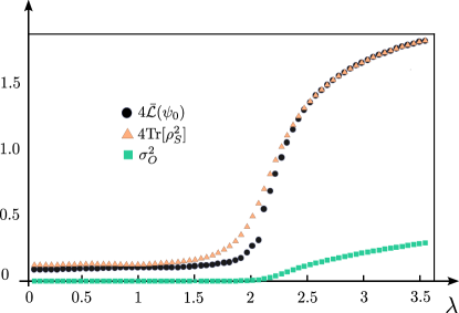
Figure 15: Observable fluctuations as a function of $\lambda$ for a chain of $n=100$ sites. We depict the observable fluctuations $\sigma_{O}^{2}$, the infinity-time average of the Loschmidt echo $\bar{\mathcal{L}}(\psi_{0})$ and the reduced subsystem purity $\Tr[\rho_{S}^{2}]$. We consider $\log(N)=9$ qubit clocks, and we take $\varepsilon=0.5$

VI.2 Diagonalization via Cartan decomposition

In this section we show how one can use the variational Hamiltonian diagonalization (to diagonalize the Hamiltonian in Eq. (48) and thus reduce the depth of the history state preparation circuit. We will take the ansatz for $D(\bm{\beta})$ and $W(\bm{\alpha})$ as appearing in Eqs. (45) and (47). Thus, as depicted in Fig. 12, $W(\bm{\alpha})$ consists of $L$ layers of two qubit gates generate by $XY$ and $YX$ arranged in a brick wall fashion, whereas the diagonal part $D(\bm{\beta})$ is just a sum of Pauli $Z$ operators on each qubit. To train the parameters $\bm{\alpha}$ and $\bm{\beta})$, we will optimize the Hilbert-Schmidt cost function defined in Eq. (35). Details of the simulation can be found in Appendix G.

We considered a chain of $n=6$ sites, and set $J=2$, and $\alpha=\frac{\sqrt{5}-1}{2}$. Moreover, we diagonalized the Hamiltonian for $\lambda=1,2,3$, thus allowing us to show the success of the algorithm in each important region of the phase diagram.

Figure 16: Variational Hamiltonian diagonalization training curves. The plot shows the decay of the loss function in Eq. (35) versus the number of training iterations. Solid lines correspond to the average over $10$ different initializations for each value of $\lambda\in\{1,2,3\}$. Shaded regions indicate the variance over the runs sample, while dash-dot lines show the best run for each batch of training runs, i.e., the one that reached the stopping value first.

Figure 17: Overparametrization transition. We show the minimum cost achieved when training the Variational Hamiltonian Diagonalization algorithm for a problem system of $n=6$ sites. The overparametrization regime is reached with a number of layers $L\geqslant 3$.

Figure 18: Testing the success of the Hamiltonian diagonalization algorithm. The left panel shows the initial “diagonalized” Hamiltonian $\hat{D}(\bm{\alpha})=W(\bm{\alpha})HW^{\dagger}(\bm{\alpha})$ where $\bm{\alpha}$ is a vector of initial random parameters $\alpha_{i}\in[0,2\pi)$. The right panel instead features $\hat{D}(\bm{\alpha}^{*})$ obtained applying the trained diagonalizing unitary to its target Hamiltonian $H$. Here $\bm{\alpha}^{*}$ are the optimal parameters of the random successful run at hand.

In Fig. 16 we show the training curves (loss function versus iteration step) for an ansatz with $L=18$ layers the three different values of $\lambda$ that we considered. Here we can clearly see that as the number of iterations increases, the cost function value goes to zero, indicating that we can accurately diagonalize the target Hamiltonian. Notably, we can see that all the trained curves converged to the solution, meaning that the optimizer did not get stuck in a local minima. Such extremely high optimization success rate can be understood from the fact that the circuit is overparametrized [98], i.e., it contains enough parameters to explore all relevant directions. In fact, using the results from [98] we know that a circuit with a set of generators $\mathcal{G}$ will be overparametrized if the number of parameters is $\leavevmode\nobreak\ \dim(\langle i\mathcal{G}\rangle_{{\rm Lie}})$. Importantly, we can use Proposition 4 to know that $\dim(\langle i\mathcal{G}\rangle_{{\rm Lie}})=n(n-1)=30$. Since the ansatz $W(\bm{\alpha})$ contains $2(n-1)$ parameters per layer (see Fig. 12), then we can overparametrize it with $L=\left\lceil n/2\right\rceil$. Indeed, in Fig. 17 we show the minimal cost achieved versus the number of layers $L$, and as expected we see a computational phase transition at $L=3$: For smaller number of layers, the ansatz is underparametrized and can get stuck in local minima, but for $L\geqslant 3$ it is overparametrized and training becomes easier. As the plot shows, once the model is overparametrized, further increasing the number of layers does not lead to any improvement in the minimum loss value achievable. Lastly, in Fig. 18 we show the success of the diagonalization by applying a successfully trained diagonalizing unitary $W(\bm{\alpha})$ to its target Hamiltonian $H$, obtaining a perfectly diagonal matrix and verifying the success of the algorithm.

VII Discussions

The simulation of quantum systems has widely been considered the most important application of quantum computation since its conception [99]. Traditionally, the focus of quantum simulations has revolved around computing quantum states and physical quantities at a given time, harnessing the exponential growth of the Hilbert space of qubits to mimic the behavior of many-body systems. However, many fundamental quantities, such as correlation functions or the equilibrium state of a quantum system, are associated with large temporal sums of the previous. In this manuscript we have shown that by treating time itself quantum mechanically, which in a computational scheme corresponds to using clock-qubits, those quantities become readily accessible.

This result arises from a fruitful analogy between the recent quantum time discussions in quantum foundations and quantum gravity fields, and the fields of quantum information and computation. More importantly, by developing quantum-time inspired algorithms, we have disclosed new important connections between the correlations contained in history states and the problem of equilibration of an isolated quantum system, thus unveiling a link to statistical mechanics as well. In particular, we have shown that the system-time entanglement is a good measure of equilibration, and as a by product, how the formalism provides a way to prepare approximate equilibrium states. Whether under proper conditions this can provide a useful scheme for studying thermalization as well is left for future investigations. These considerations show that, in addition to the practical applications of the various proposed algorithms, the framework we presented offers new insights that can be applied to diverse areas of many-body physics.

The system-time entanglement is also indicative of the need for entangling gates to prepare history states. In this work we have considered a fixed architecture which even for a direct Trotterization approach provides an exponential advantage over sequential in time schemes. We have also considered a further simplification via a variational Hamiltonian diagonalization approach. Interestingly, the fact that the entanglement is state and evolution dependent suggest that one can consider more adaptive preparation schemes, where the entanglement is used as a measure of “compressibility” (or complexity) of the history state. While we leave the study of these possibilities for future investigations, we should mention that a global variational scheme has been proposed recently [30] based on the Feynman-Kitaev Hamiltonian [6]. As with any variational protocol, knowledge of the structure of the solution is valuable for choosing proper ansatzes, thus rendering our efficient protocol particularly relevant for any near-term implementation as well. At the same time, all of our protocols can be easily updated by replacing the history state preparation subroutine. The newly disclosed parallel-in-time advantages clearly hold and can be readily extended to any related proposal including [30].

In all the protocols we have considered, the circuits give information about the history of a closed system. However, these protocols can be extended to consider the history of states which at some points in time are being subject to measurements. This becomes feasible by following the recent treatment of Ref. [7] that incorporates ancillary memories (following Von Neumann) and describe the history of the whole (history of the system+ancillas). This framework opens many new interesting possibilities for novel quantum algorithms. A similar treatment may be applied to quantum evolutions associated to non-unitary channels (open systems).

On the other hand, even if we focus in closed systems there is much to explore yet: most of the parallel protocols in the paper involve measurements on the system side. We also know that adding a projective measurement in the time basis of the clocks qubits yields predictions at a given time. However, the most characteristic features of quantum mechanics arise when one is considering measurements in different bases meaning that the full potential of quantum time effects still need to be explored. In addition, multiple copies of history states may be used to study higher momenta of mean values, thus opening even more possibilities. Going even further, it has been recently discussed [12, 13, 14, 31] that the PaW formalism is not enough for achieving a fully symmetric version of quantum mechanics. Hence, we can speculate that in the near future, and motivated by the current results, these and other proposals may allow to provide further informational and computational insights related to the time domain.

Appendices for “Parallel-in-time quantum simulation via Page and Wootters quantum time”

Here we present derivations, additional details for the main results, and further general discussions on quantum time notions. The appendices are organized as follows: In Appendix A we give an overview of quantum time approaches and describe connections between our work and the literature. In Appendix B we explain in more detail the relation between quantum time and the equilibration problem and prove the related Theorems in the main body. In Appendix C we give detailed proofs of all the different circuits we proposed in the main body. In Appendix D we prove Theorem 5 about circuit depths in the sequential and parallel-in-time schemes. In Appendix E we prove Proposition 4 about the algebra of the $XY$ model. In Appendix F we prove Theorem 7 regarding the depth of the total protocols involving both Hamiltonian diagonalization and history states. Finally, in Appendix G we provide details about the methods employed in the numerics (sec. VI).

Appendix A Connection to literature and Overview of Quantum Time approaches

Here we briefly discuss the broader conceptual picture of “quantum time-related proposals”. This should also clarify the range of applicability of our current ideas. Regarding the Page and Wootters approach [38], it is worth noting that their original idea was to replace dynamics with quantum correlations. The physical picture was a static universe from which evolution emerges from a convenient separation between the system, and the rest. In this sense the “time” Hilbert space corresponds to a “cosmological” clock. One main motivation for these ideas was the discussion about time in quantum gravity [36], where the Wheeler-deWitt equation [102] suggests a static universe. Such equation appears as a constraint induced by the “gauge” freedom in the choice of coordinates in general relativity, and can be understood within the framework of Dirac’s generalization of Hamiltonian dynamics to constrained systems [103, 104].

However, there are important conceptual and mathematical differences between the PaW’s and Dirac’s approaches which are at the core of our ability to leverage the first and not the second to develop useful computational schemes. To clarify this statement, let us briefly discuss a simple but archetypal application of Dirac’s approach: in classical mechanics, one can accommodate time itself and its conjugate variable $p_{t}$ in an extended phase-space by introducing a new variable $\tau$ which parametrizes phase-space variables, including $t=t(\tau)$, $p_{t}=p_{t}(\tau)$. The Poisson brackets are also extended by imposing $\{t,p_{t}\}=1$ with $p_{t}\neq H$ which for a single particle and $x^{0}\equiv t$, $p_{t}\equiv p_{0}$ completes the algebra $\{x^{\mu},p_{\nu}\}=\delta^{\mu}_{\;\nu}$, which now is explicitly covariant. Part of the quantization scheme now consists of the replacement

$$\{x^{\mu},p_{\nu}\}=\delta^{\mu}_{\;\nu}\to[x^{\mu},p_{\nu}]=i\hbar\delta^{\mu}_{\;\nu}$$ (50)

which for $\mu=\nu=0$ is just $[T,P_{T}]=i\hbar$ (when the system is a particle), i.e. $x^{0}\equiv T$ with $[T,H]=0$ for $H$ some Hamiltonian of the particle. On the other hand, the independence of physical quantities on the way the $\tau$-parametrization is chosen leads to $\mathcal{J}|\Psi\rangle=0$ after quantization. This reparametrization invariance is analogous to the general covariance of general relativity, and the constraint is analogous to the Wheeeler-deWitt equation.

However, contrary to our main body discussion, in Dirac’s approach the constraint equation defines the so-called physical Hilbert space which is regarded as different from the previous “kinematic” Hilbert space. Moreover, the physical Hilbert space is not treated as a subspace of the latter, instead the kinematical one appears only as an auxiliary step in the whole quantization process but not in the final construction. As a consequence, the time operator is ruled out in the final formalism for not being a physical observable (see e.g. [106] for discussions about this procedure and the related “Hilbert space problem”). As we have shown in the main body, in the PaW approach the interpretation and treatment of the constraint are completely different: the time operator is not disregarded since it corresponds to an actual observable of the clock system. The complete Hilbert space e.g. as defined by (50) is preserved, while the state of the system is recovered by conditioning . The theoretical ideas underlying our manuscript clearly exploit the “extended” Hilbert space associated with the PaW approach and are mostly inspired by the recent developments in the context of quantum information [7, 8, 11, 12], and in particular in the discrete-time formulation [8], which was further extended in [9].

Let us also stress that in for the purposes of our manuscript it is not relevant whether explicit covariance is achieved via the definition of a time operator. This means that we can consider arbitrary many-body systems as we have shown in the main body. This also includes relativistic systems (properly discretized quantum field theories) but their simulation corresponds to the evolution as seen from a fixed reference frame: in this case there is no simple rule to relate a history state in a given reference frame to another. In this sense, we regard the PaW formalism as non-explicitly-relativistic. There is however a simple situation where such rule is straightforward: for a single relativistic particle Lorentz transformations can be introduced explicitly and geometrically (as space-time “rotations” independently of the theory) [11, 12]. For this to be actually achieved one needs to preserve the kinematical space and deal with an extended inner product, a result which is again highlighting the advantages of the extended scheme. This approach was recently developed in [11] for Dirac’s particles and in [12] for scalar particles where the new inner products were successfully related to the “physical” ones while preserving the extended Hilbert spaces. As a consequence, the associated history states can still be realized by the means presented in this manuscript (adopting some discretization of space-time), and in principle, Lorentz transformations may be introduced as non-local gates acting on both the system and time qubits.

Another interesting feature of these single-particle quantum time formalisms (which preserve the extended Hilbert space) is that their “second quantization”, as introduced in [12, 13, 14] naturally leads to a new approach to many-body scenarios and to quantum field theories in which space and time are explicitly on equal footing (see also the closely related “quantum mechanics of events” proposal [31]). In particular, the approach in [13] also leads to a redefinition of the Path Integral formulation [14]. In fact, the real challenge to treat space and time on equal footing at the Hilbert space level in relativistic settings has to do with another more subtle asymmetry in the treatment of time [40, 108, 13, 14]: joint systems separated in space are described by the tensor product of the corresponding Hilbert spaces. No such rule is applied to time. This asymmetry is particularly evident in the case of quantum field theories, in which case space is treated as a site, which e.g. for bosons is equivalent to a tensor product structure in space. While time is a parameter, it is not a site index and there is no associated tensor product structure. This is manifest in the equal time canonical algebra imposed on the fields which requires a fixed foliation. We notice also that this is an obstacle in defining a notion of “time-like entanglement” (see however [13, 14, 109, 110, 111] for recent related discussions), a consideration which applies to all QM: the previous asymmetry is present in any quantum mechanical system, as also discussed in [40, 112, 10, 42, 13, 14].

For these reasons, it is not sufficient to define a quantum time operator to solve “the problem of time” or more precisely to have an explicit space-time symmetric version of QM. This renders the aforementioned second quantization of “PaW particles” particularly interesting. While its description clearly exceeds the purpose of this manuscript, we can speculate that these developments may provide additional quantum computational and informational tools, just as the PaW approach inspired the various algorithms of our manuscript.

Appendix B More on the Relation between Quantum Time and the Equilibration Problem: Proof of Theorem 3

In this section we highlight the relations between the current quantum time approach (the PaW-inspired formalism), its associated concept of system-time entanglement, and the problem of equilibration of an isolated quantum system. In particular, we provide a prove and analysis of Theorem 3. Let us mention that this connection has not been explored in the literature (see however the recent article [26]).

Let us recall first that a system is said to equilibrate if it evolves towards some particular in general mixed state and remains in that state or close to it for almost all times [53]. More precisely, this holds for either a small subsystem of a large quantum system evolving unitarily [53] (subsystem equilibration), or for expectation values associated with “experimentally realistic conditions” [4] (observable equilibration). The last interpretation refers to the fact that the probability that mean values computed with $\ket{\psi(t)}\!\bra{\psi(t)}$ differ from mean values computed with the equilibrium state becomes exponentially vanishing for typical experimentally accessible observables [4, 113]. In both scenarios, the dephased state $\bar{\rho}$ defined in Eq. (17) plays a central role since it is identified with the equilibrium state (equivalently, the subsystems equilibrium state is a partial trace of this global state). Moreover, the theoretical bound [4] used to prove this is related to $\bar{\mathcal{L}}$ precisely because $\Tr[\bar{\rho}^{2}]=\bar{\mathcal{L}}\,,$ i.e. the purity of the time-averaged state is $\bar{\mathcal{L}}$. The same quantity provides a bound for the (time average of) the distance between the subsystem state and (the partial trace of) $\bar{\rho}$ [53].

Now returning to the history state, we have seen that the quadratic entanglement involves the purity of $\rho_{S}=\Tr_{T}[|\Psi\rangle\langle\Psi|]$. The explicit expansion of $\rho_{S}$ is

$$\rho_{S}=\frac{1}{N}\sum_{t}|\psi(\varepsilon t)\rangle\langle\psi(\varepsilon t)|\,.$$ (51)

In order to relate this state with $\bar{\rho}$ we can use the energy basis $|k\rangle$ so that $H|k\rangle=E_{k}|k\rangle$. Any initial state has an expansion $|\psi_{0}\rangle=\sum_{k}c_{k}|k\rangle$. Notice that even if there is degeneracy we can always write a fixed pure state as before, with $|c_{k}|^{2}:=\sum_{j}|\psi_{kj}|^{2}\,,\;\;\;|k\rangle:=c_{k}^{-1}\sum_{j}\psi_{kj}|kj\rangle\,,$ and $H|kj\rangle=E_{k}|kj\rangle$, i.e. $j$ is a degeneracy index. The quantity $c_{k}|k\rangle$ is the projection of $|\psi\rangle$ onto the subspace of states with energy $E_{k}$. Thus we obtain

$$\rho_{S}=\frac{1}{N}\sum_{t}\sum_{k,k^{\prime}}c_{k}c_{k^{\prime}}^{\ast}e^{-i(E_{k}-E_{k^{\prime}})t\varepsilon}|k\rangle\langle k^{\prime}|\,,$$ (52)

which is precisely the discrete time version of $\bar{\rho}$ as defined in Eq. 17, i.e.

$$\rho_{S}=\tilde{\rho}\,.$$ (53)

Notice that while the purity of $\bar{\rho}$ coincides with $\bar{\mathcal{L}}$, the purity of $\rho_{S}$ is not $\widetilde{\mathcal{L}}$. Remarkably, the natural discrete-time generalization of $\bar{\mathcal{L}}=\Tr[\bar{\rho}^{2}]$ is $\Tr[\rho_{S}^{2}]$ and not $\widetilde{\mathcal{L}}$: the system-time entanglement provides the proper discrete-time version of time average related bounds (it is worth remarking that the discrete-time entanglement provides strict bounds to the infinite and continuum time averages). This is captured by Theorem 3 and its corollaries.

We are now in a position to give the proof of Theorem 3:

Proof.

Let us first rewrite $\rho_{S}$ as

$$\rho_{S}=\sum_{k,k^{\prime}}c_{k}c_{k^{\prime}}^{\ast}\Delta_{kk^{\prime}}|k\rangle\langle k^{\prime}|\,,$$ (54)

with $\Delta_{kk^{\prime}}:=\frac{1}{N}\sum_{t}e^{-i(E_{k}-E_{k^{\prime}})t\varepsilon}$. Notice that $\Delta_{kk}=1$. Being a quantum state, we can diagonalize $\rho_{S}$ in some basis as

$$\rho_{S}=\sum_{l}p_{l}|l\rangle\langle l|\,.$$ (55)

In fact, it is clear that this is what is obtained by tracing over the clocks with $|\Psi\rangle$ in its Schmidts decomposition (15).

We can combine these two expansions to write

$$\langle k|\rho|k\rangle=|c_{k}|^{2}=\sum_{l}p_{l}|\langle l|k\rangle|^{2}\,.$$ (56)

The quantity $|\langle l|k\rangle|^{2}$ defines a double stochastic matrix thus yielding the desired majorization relation

$$\{|c_{k}|^{2}\}\prec\{p_{l}\}$$ (57)

thus implying the desired majorization relation between states (we recall that $\bar{\rho}=\sum_{k}|c_{k}|^{2}|k\rangle\langle k|$). Notice that similar ideas have been used in [8].

It is also clear that by taking the limits $\varepsilon\to 0$ and then $T\to\infty$ the energy dephasing is recovered: the first limit can be considered by writing

$$\Delta_{kk^{\prime}}=\frac{1}{\varepsilon N}\sum_{t}\varepsilon\,e^{-i(E_{k}-E_{k^{\prime}})t\varepsilon}\to\int_{0}^{T}\frac{dt}{T}e^{-i(E_{k}-E_{k^{\prime}})t}\,,$$

with $dt\equiv\varepsilon$. The large $T$ limit now is the familiar limit used conventionally (which yields a delta), thus leading again to the asymptotic relation

$$\rho_{S}\to\bar{\rho}\,.$$ (58)

Instead, in the periodic case we can use the fact that the periodicity condition requires $E_{k}\equiv E_{l_{k}}=2\pi l_{k}/T$ for $l_{k}$ an integer. This means that

$$\Delta_{kk^{\prime}}=\frac{1}{N}\frac{1-e^{i(E_{k}-E_{k^{\prime}})T}}{1-e^{i(E_{k}-E_{k^{\prime}})\varepsilon}}=\delta_{kk^{\prime}}$$

with the last equality holding only in the periodic case. By replacing this in Eq. (55) we obtain precisely $\rho_{S}=\bar{\rho}$.

∎

Notice that the Corollaries 1 and 2 follow immediately from the Schur-concavity of functions defining any entropy. These Corollaries are the particular case of the linear entropy. Interestingly, new bounds can be obtained by just considering other entropies.

Let us also make more precise the main body statement that the quantum time formalism gives a new interpretation to the loss of coherences induced by a time average: as we said, since the system is “entangled with time”, by ignoring the “clock qubits” we lose information. For discrete time, the information loss induces $\rho\to\tilde{\rho}$ which is a quantum channel with Krauss operators $K_{t}:=e^{-iHt\varepsilon}/\sqrt{N}$ such that

$$\tilde{\rho}=\sum_{t}K_{t}^{\dagger}\rho K_{t}\,.$$ (59)

As usual this quantum channel can be purified by using the isometric extension [114] $U[K_{t}]:=\sum_{t}|t\rangle\otimes K_{t}$ so that the channel is recovered by tracing over the “environment” (here the clock) in a global state $U[K_{t}]|\psi\rangle$. This global state is precisely the history state of Eq. (4), i.e.,

$$|\Psi\rangle=U[K_{t}]|\psi_{0}\rangle\,.$$ (60)

We see that one can “rediscover” the quantum time formalism from the natural purification of the channel (59). Just as in the general case, where a nontrivial channel is induced by correlations between the system and an environment, the system is correlated (entangled) with time. Moreover, the quantum channel’s theory [114] implies that there is a unitary $V$ such that

$$|\Psi\rangle=V|0\rangle\otimes|\psi\rangle\,.$$ (61)

One possible unitary is provided by the circuit of figure 2. We should remark however that the operation of tracing over the clock degrees of freedom is very different from measuring on the clock register and conditioning the state of the system. When conditioning one has access to the clock, as it is required for implementing a projection at a given time state. In summary, the history state contains both information about evolution at specific times, recovered from conditioning, and about the “equilibration channel” (59), recovered by ignoring the clock.

Appendix C Proofs involving circuits

C.1 Proof of Proposition  1

Proof.

Consider the circuit in Fig. 4. For ease of calculation, we will assume that $\rho=\ket{\psi_{0}}\!\bra{\psi_{0}}$, for some initial state $\ket{\psi_{0}}$. Moreover, we recall that both $O_{1}$ and $O_{2}$ are Pauli operators. The input state to the circuit is $\ket{\psi_{0}}\ket{0}$, where the single qubit state initialized in the zero state is an ancilla used to perform a Hadamard test. The action of the Hadamard gates is to map

$$\ket{\psi_{0}}\ket{0}\rightarrow\ket{\psi_{0}}\ket{+}\,.$$ (62)

Assuming the colored dashed gate in Fig. (4) is an identity, we next have a controlled $O_{2}$ operation. This produces the state

$$\ket{\psi_{0}}\ket{+}\rightarrow\frac{1}{\sqrt{2}}(\ket{\psi_{0}}\ket{0}+O_{2}\ket{\psi_{0}}\ket{1})\,.$$ (63)

Next, in the $t$-th experiment, we evolve the state with a unitary $U(\varepsilon t)$, leading to

$$\frac{1}{\sqrt{2}}(\ket{\psi_{0}}\ket{0}+O_{2}\ket{\psi_{0}}\ket{1})\rightarrow\frac{1}{\sqrt{2}}(U(\varepsilon t)\ket{\psi_{0}}\ket{0}+U(\varepsilon t)O_{2}\ket{\psi_{0}}\ket{1})\,.$$ (64)

The next controlled $O_{1}$ gate leads to

$$\frac{1}{\sqrt{2}}(U(\varepsilon t)\ket{\psi_{0}}\ket{0}+U(\varepsilon t)O_{2}\ket{\psi_{0}}\ket{1})\rightarrow\frac{1}{\sqrt{2}}(U(\varepsilon t)\ket{\psi_{0}}\ket{0}+O_{1}U(\varepsilon t)O_{2}\ket{\psi_{0}}\ket{1})\,.$$ (65)

The final Hadamard gate produces the state

$$\frac{1}{\sqrt{2}}(U(\varepsilon t)\ket{\psi_{0}}\ket{0}+O_{1}U(\varepsilon t)O_{2}\ket{\psi_{0}}\ket{1})\rightarrow \frac{1}{2}(U(\varepsilon t)\ket{\psi_{0}}(\ket{0}+\ket{1})+O_{1}U(\varepsilon t)O_{2}\ket{\psi_{0}}(\ket{0}-\ket{1}))$$

$$= \frac{1}{2}\left((U(\varepsilon t)\ket{\psi_{0}}+O_{1}U(\varepsilon t)O_{2}\ket{\psi_{0}})\ket{0}+(U(\varepsilon t)\ket{\psi_{0}}-O_{1}U(\varepsilon t)O_{2}\ket{\psi_{0}})\ket{1}\right)\,.$$ (66)

Then, probability of measuring the ancilla qubit in the zero state is

$$p(0) =\frac{1}{4}\left((\bra{\psi_{0}}U^{\dagger}(\varepsilon t)+\bra{\psi_{0}}O_{2}U^{\dagger}(\varepsilon t)O_{1})\bra{0}+(\bra{\psi_{0}}U^{\dagger}(\varepsilon t)-\bra{\psi_{0}}O_{2}U^{\dagger}(\varepsilon t)O_{1})\bra{1}\right)$$

$$\quad\cdot\left((U(\varepsilon t)\ket{\psi_{0}}+O_{1}U(\varepsilon t)O_{2}\ket{\psi_{0}})\ket{0}+(U(\varepsilon t)\ket{\psi_{0}}-O_{1}U(\varepsilon t)O_{2}\ket{\psi_{0}})\ket{1}\right)$$

$$=\frac{1}{4}\sum_{t=0}^{N-1}(2+\bra{\psi_{0}}U^{\dagger}(\varepsilon t)O_{1}U(\varepsilon t)O_{2}\ket{\psi_{0}}+\bra{\psi_{0}}O_{2}^{\dagger}U^{\dagger}(\varepsilon t)O_{1}^{\dagger}U(\varepsilon t)\ket{\psi_{0}})$$

$$=\frac{1}{2}(1+\text{Re}[\langle O_{1}(t)O_{2}\rangle_{\psi_{0}}])\,.$$ (67)

Similarly, the probability of measuring the ancilla qubit in the one state is

$$p(1) =\frac{1}{2}(1-\text{Re}[\langle O_{1}(t)O_{2}\rangle_{\psi_{0}}])\,.$$ (68)

Combining Eqs. (67) and (68) shows that the expectation value of the $Z$ operator on the ancilla qubit is

$$\langle Z\rangle=p(1)-p(0) =\text{Re}[\langle O_{1}(t)O_{2}\rangle_{\psi_{0}}]\,.$$ (69)

By adding, an $S^{\dagger}$ gate in place of the colored dashed gate in Fig. 4 one finds

$$\langle Z\rangle=\text{Im}[\langle O_{1}(t)O_{2}\rangle_{\psi_{0}}]\,.$$ (70)

Since this procedure needs to be repeated $N$ times, and since we want to estimate the expectation values up to precision $\delta$, then one needs to perform $\mathcal{O}(N/\delta^{2})$ experiments. ∎

C.2 Proof of Theorem 1

Proof.

Consider the circuit in Fig. 5. For ease of calculation, we will assume that $\rho=\ket{\psi_{0}}\!\bra{\psi_{0}}$ for some initial state $\ket{\psi_{0}}$. We also recall that both $O_{1}$ and $O_{2}$ are Pauli operators. The input state to the circuit is $\ket{0}^{\log{N}}\ket{\psi_{0}}\ket{0}$, where we recall that $\ket{0}^{\log{N}}$ is the initial state of the clock-qubits. The action of the Hadamard gates is to map

$$\ket{0}^{\log{N}}\ket{\psi_{0}}\ket{0}\rightarrow\frac{1}{\sqrt{N}}\sum_{t=0}^{N-1}\ket{t}\ket{\psi_{0}}\ket{+}\,.$$ (71)

Here we have used the identity $\ket{+}^{\log(N)}=\frac{1}{\sqrt{N}}\otimes_{j=1}^{\log{N}}(\ket{0_{j}}+\ket{1_{j}})=\frac{1}{\sqrt{N}}\sum_{t=0}^{N-1}\ket{t}$ which follows by expressing $t$ in its binary form $t=\sum_{j=1}^{\log{N}}t_{j}2^{j-1}$. Assuming the colored dashed gate in Fig. 5 is an identity, we next have a controlled $O_{2}$ operation. This produces the state

$$\frac{1}{\sqrt{N}}\sum_{t=0}^{N-1}\ket{t}\ket{\psi_{0}}\ket{+}\rightarrow\frac{1}{\sqrt{2N}}\sum_{t=0}^{N-1}\ket{t}(\ket{\psi_{0}}\ket{0}+O_{2}\ket{\psi_{0}}\ket{1})\,.$$ (72)

Next, the sequence of $\log{N}$ controlled gates $U(2^{j-1}\frac{T}{N})=U(\frac{T}{N})^{2^{j-1}}$ for $j=1,\ldots,\log{N}$ perform the operations

$$\frac{1}{\sqrt{2N}}\sum_{t=0}^{N-1}\ket{t}(\ket{\psi_{0}}\ket{0}+O_{2}\ket{\psi_{0}}\ket{1})\rightarrow\frac{1}{\sqrt{2N}}\sum_{t=0}^{N-1}\ket{t}(U(\varepsilon t)\ket{\psi_{0}}\ket{0}+U(\varepsilon t)O_{2}\ket{\psi_{0}}\ket{1})\,.$$ (73)

The next controlled $O_{1}$ gate leads to

$$\frac{1}{\sqrt{2N}}\sum_{t=0}^{N-1}\ket{t}(U(\varepsilon t)\ket{\psi_{0}}\ket{0}+U(\varepsilon t)O_{2}\ket{\psi_{0}}\ket{1})\rightarrow\frac{1}{\sqrt{2N}}\sum_{t=0}^{N-1}\ket{t}(U(\varepsilon t)\ket{\psi_{0}}\ket{0}+O_{1}U(\varepsilon t)O_{2}\ket{\psi_{0}}\ket{1})\,,$$ (74)

while the controlled phase gates perform the map

$$\frac{1}{\sqrt{2N}}\sum_{t=0}^{N-1}\ket{t}(U(\varepsilon t)\ket{\psi_{0}}\ket{0}+O_{1}U(\varepsilon t)O_{2}\ket{\psi_{0}}\ket{1})\rightarrow\frac{1}{\sqrt{2N}}\sum_{t=0}^{N-1}(\ket{t}U(\varepsilon t)\ket{\psi_{0}}\ket{0}+e^{-it}\ket{t}O_{1}U(\varepsilon t)O_{2}\ket{\psi_{0}}\ket{1})\,.$$ (75)

The final Hadamard gate gives rise to

$$\frac{1}{\sqrt{2N}}\sum_{t=0}^{N-1}(\ket{t}U(\varepsilon t)\ket{\psi_{0}}\ket{0}+e^{-i\omega\varepsilon t}\ket{t}O_{1}U(\varepsilon t)O_{2}\ket{\psi_{0}}\ket{1})\rightarrow \frac{1}{2\sqrt{N}}\sum_{t=0}^{N-1}(\ket{t}U(\varepsilon t)\ket{\psi_{0}}(\ket{0}+\ket{1})+e^{-i\omega\varepsilon t}\ket{t}O_{1}U(\varepsilon t)O_{2}\ket{\psi_{0}}(\ket{0}+\ket{1}))$$

$$= \frac{1}{2\sqrt{N}}\sum_{t=0}^{N-1}(\ket{t}U(\varepsilon t)\ket{\psi_{0}}+e^{-i\omega\varepsilon t}\ket{t}O_{1}U(\varepsilon t)O_{2}\ket{\psi_{0}})\ket{0}$$

$$+(\ket{t}U(\varepsilon t)\ket{\psi_{0}}-e^{-i\omega\varepsilon t}\ket{t}O_{1}U(\varepsilon t)O_{2}\ket{\psi_{0}})\ket{1}\,.$$ (76)

Thus, the probability of measuring the ancilla qubit in the zero state is

$$p(0) =\frac{1}{4N}\sum_{t=0}^{N-1}\sum_{t^{\prime}=0}^{N-1}(\bra{t^{\prime}}\bra{\psi_{0}}U^{\dagger}(t^{\prime})+e^{i\omega\varepsilon t^{\prime}}\bra{t^{\prime}}\bra{\psi_{0}}O_{2}^{\dagger}U^{\dagger}(t^{\prime})O_{1}^{\dagger})(\ket{t}U(\varepsilon t)\ket{\psi_{0}}+e^{-i\omega\varepsilon t}\ket{t}O_{1}U(\varepsilon t)O_{2}\ket{\psi_{0}})$$

$$=\frac{1}{4N}\sum_{t=0}^{N-1}(2+e^{-i\omega\varepsilon t}\bra{\psi_{0}}U^{\dagger}(\varepsilon t)O_{1}U(\varepsilon t)O_{2}\ket{\psi_{0}}+e^{i\omega\varepsilon t}\bra{\psi_{0}}O_{2}^{\dagger}U^{\dagger}(\varepsilon t)O_{1}^{\dagger}U(\varepsilon t)\ket{\psi_{0}})$$

$$=\frac{1}{2}(1+\text{Re}[\widetilde{F}(O_{1},O_{2},\omega)])\,.$$ (77)

Similarly, the probability of measuring the ancilla qubit in the one state is

$$p(1) =\frac{1}{2}(1-\text{Re}[\widetilde{F}(O_{1},O_{2},\omega)])\,.$$ (78)

Combining Eqs. (77) and (78) shows that the expectation value of the $Z$ operator on the ancilla qubit is

$$\langle Z\rangle=p(1)-p(0) =\text{Re}[\widetilde{F}(O_{1},O_{2},\omega)]\,.$$ (79)

By adding, an $S^{\dagger}$ gate in place of the colored dashed gate in Fig. 5 one finds

$$\langle Z\rangle=\text{Im}[\widetilde{F}(O_{1},O_{2},\omega)]\,.$$ (80)

If, one wishes to estimate $\langle Z\rangle$ up to precision $\delta$, then one needs to perform $\mathcal{O}(1/\delta^{2})$ measurements. This results in $\mathcal{O}(1/\delta^{2})$ experiments. ∎

C.3 Proof of Proposition 2

Proof.

Consider the circuit in Fig. 6. We can readily see that the circuit therein is nothing but the circuit for computing the overlap between two quantum state $\rho$ and $\sigma$ derived in Ref. [43] and also shown in Sup. Fig. 1.

Supplementary Figure 1: Algorithm for computing the overlap between two quantum states. We show an algorithm which takes as input two arbitrary $n$-qubit quantum states $\rho$ and $\sigma$ and which estimates the overlap $\Tr[\rho\sigma]$. In a) we show the algorithm for the case when $\rho$ and $\sigma$ and single qubit states, and in b) the generalization for larger qubit sizes. We can see that in all cases the circuit depth is equal to two, and hence independent of $n$.

To understand the algorithm of Ref. [43], let us consider first the case of $\rho$ and $\sigma$ being single qubit states. We know that the following identity holds

$$\Tr[\rho\sigma]=\Tr[(\rho\otimes\sigma){\rm SWAP}]\,,$$ (81)

where ${\rm SWAP}$ denotes the SWAP operator, whose action can be defined in the computational basis as ${\rm SWAP}\ket{ij}=\ket{ji}$. Then, let us define the Bell basis:

$$\ket{\Phi_{1}}=\frac{1}{\sqrt{2}}(\ket{01}+\ket{10})\,,\quad\ket{\Phi_{2}}=\frac{1}{\sqrt{2}}(\ket{00}+\ket{11})\,,\quad\ket{\Phi_{3}}=\frac{1}{\sqrt{2}}(\ket{00}-\ket{11})\,,\quad\ket{\Phi_{4}}=\frac{1}{\sqrt{2}}(\ket{01}-\ket{10})\,.$$ (82)

It is not hard to see that the SWAP operator is diagonal in the Bell basis, and that it can be expressed as

$${\rm SWAP}=\ket{\Phi_{1}}\!\bra{\Phi_{1}}+\ket{\Phi_{2}}\!\bra{\Phi_{2}}+\ket{\Phi_{3}}\!\bra{\Phi_{3}}-\ket{\Phi_{4}}\!\bra{\Phi_{4}}\,.$$ (83)

Thus, we can estimate the expectation value of the SWAP operator over the state $\rho\otimes\sigma$

$$\langle{\rm SWAP}\rangle_{\rho\otimes\sigma}=\Tr[(\rho\otimes\sigma){\rm SWAP}]=P(\Phi_{1})+P(\Phi_{2})+P(\Phi_{3})-P(\Phi_{4})\,,$$ (84)

where here we defined the probabilities $P(\Phi_{i})=\langle\Phi_{i}|\rho\otimes\sigma|\Phi_{i}\rangle$. That is, $P(\Phi_{i})$ denotes the probability of measuring the state $\rho\otimes\sigma$ in the Bell basis, and obtaining the measurement outcome $\ket{\Phi_{i}}$. This result shows that we cane estimate $\Tr[\rho\sigma]$ by preparing $\rho\otimes\sigma$ and measuring in the Bell basis. Crucially, one can readily prove the such a measurement can be performed with the circuit in Sup. Fig. 1(a), which is composed of a $CNOT$ gate and a Hadamard gate in the first qubit (i.e., with the inverse of the circuit used to prepare a Bell state).

A similar result will follow when $\rho\otimes\sigma$ are $n$-qubit states, but now one has to measure the expectation value of the operator $\prod_{j=1}^{n}{\rm SWAP}_{j_{A},j_{B}}$, where here ${\rm SWAP}_{j_{A},j_{B}}$ denotes the operator that swaps the $j$-th qubit of $\rho$ with the $j$-th qubit of $\sigma$. Since each operator ${\rm SWAP}_{j_{A},j_{B}}$ can be expanded in a (local) Bell basis, the circuit used to measure in the eigenbasis of $\prod_{j=1}^{n}{\rm SWAP}_{j_{A},j_{B}}$, and hence to estimate $\Tr[\rho\sigma]$ is precisely that which is shown in Sup. Fig. 1(b). Finally, since we are computing an expectation value, if we want to reach a precision $\delta$ for each $N$, we need to run $\mathcal{O}(N/\delta^{2})$ experiments.

∎

C.4 Proof of Theorem 2

Proof.

The proof of this theorem follows very closely that of Proposition 2. In particular, we can see from Fig. 7 that we are performing a SWAP test, i.e., measuring the overlap via Bell basis measurements, between the reduced state $\rho_{S}$ of the history state on the system qubits, and the state $\ket{\psi_{0}}\!\bra{\psi_{0}}$. On the other hand, one can readily see by expanding $\rho_{S}$ as in Eq. (51) that the overlap between $\rho_{S}$ and $\ket{\psi_{0}}\!\bra{\psi_{0}}$ is precisely $\widetilde{\mathcal{L}}(\psi_{0})$. Hence, we can use the circuit in Fig. 7 to estimate $\widetilde{\mathcal{L}}(\psi_{0})$ up to $\delta$ precision with $\mathcal{O}(1/\delta^{2})$ experiments.

∎

Appendix D Proof of Theorem 5

Proof.

Let us remark first that the gates we consider here are only those directly related to implementing the unitary evolution. The other parts of the circuit are common to both the sequential and parallel in time approaches, meaning that it is advantageous to have less runs (thus the parallel approach is always more convenient). The only exception is when we add the phases in Figure 5 but this only adds $\log(N)$ gates which is negligible in this analysis. A fully explicit depth analysis taking into account all gates for each circuit is provided in Appendix F in the context of the variational diagonalization scheme.

Let us discuss first the conventional sequential approach. The maximum number of gates one requires in a single run is the “last one” corresponding to $U(T)$. In this case, one needs $\#_{g}(T)\in\gamma lT^{\alpha}$ gates. A more relevant quantity is the total number of gates $\#^{\text{seq}}$ one needs to implement since this will determine the actual computational time. By summing over the amount of gates of each run one obtains

$$\#^{\text{seq}}=\gamma l\sum_{t=1}^{N-1}(\varepsilon t)^{\alpha}\in\gamma l\mathcal{O}(N^{\alpha+1})\,,$$ (85)

where we retain the information on $l$ for a proper comparison.

Now let us consider the parallel-in-time approach. In this scheme each $U(t)$ is first “Trotterized” and each individual gate is controlled. This gives an additional overall multiplicative factor proportional to $l$ , say $\beta l$. For local Hamiltonians, this is logarithmic in the system size. On the hand, the parallelization reduces the number of evolution gates exponentially. The total number of gates $\#^{\text{par}}$ is in fact now

$$\#^{\text{par}}=\gamma\beta l^{2}\sum_{j=0}^{\log(N)-1}(\varepsilon 2^{j})^{\alpha}\in\beta\gamma l^{2}\mathcal{O}(N^{\alpha})\,.$$ (86)

Notice that contrary to the sequential case, in the parallel in time scheme we sum over a logarithmic amount of times, with $U(T/2)$ the gate with the longest evolution in the whole protocol ($T/2=\varepsilon 2^{\log(N)-1}$). By comparing the previous equations the last part of the Theorem immediately follows.

∎

Appendix E Proof of proposition 4

Proof.

Note that $\mathfrak{k}$ admits a bodyness-graded basis

$$B=\bigcup_{k=2}^{n}B_{k}\,,\quad\text{where $B_{k}=\{\widehat{X_{i}Y}_{i+k-1},\widehat{Y_{i}X}_{i+k-1}\}_{i=1}^{n-k}$}$$ (87)

Clearly, $|B_{k}|=2(n-k)$ and $2\sum_{k=2}^{n}(n-k)=2{n\choose 2}=n(n-1)=\dim(\mathfrak{k})$. The claim is that the set $B_{2}\subset B$ generates $\mathfrak{k}$.

We prove this by induction. First we show $B_{2}$ generates $B_{3}$. For all $i\in 1,\ldots,n-2$ we obtain each element in $B_{3}$ from

$$[X_{i}Y_{i+1},X_{i+1}Y_{i+2}]\propto X_{i}Z_{i+1}Y_{i+2}$$ (88)

$$[Y_{i}X_{i+1},Y_{i+1}X_{i+2}]\propto Y_{i}Z_{i+1}Z_{i+2}$$ (89)

Now lets see that, in general, $B_{2}$ and $B_{k}$ suffice to generate $B_{k+1}$. Specifically, each element in $B_{k+1}$ follows from

$$[X_{i}Y_{i+1},\widehat{X_{i+1}Y}_{i+k-1}]\propto\widehat{X_{i}Y}_{i+k}$$ (90)

$$[Y_{i}X_{i+1},\widehat{Y_{i+1}X}_{i+k-1}]\propto\widehat{Y_{i}X}_{i+k}$$ (91)

for $i\in 1\ldots n-(k-1)$. ∎

Appendix F Proof of Theorem 7

Proof.

In what follows we will assume that the history state preparation subroutine is replaced as in Fig. 11 where $W$ and $D$ are respectively given by the optimized ansatzes $W(\bm{\alpha})$ and $W(\bm{\beta})$. Moreover, we recall from Ref. [90] that for $W(\bm{\theta})$ to be overparametrized it needs a number of parameters in $\mathcal{O}(\dim(\mathfrak{k}))=\mathcal{O}(n^{2})$. Since the ansatz in Eq. (47) has $(2n-2)$ parameters per layer (see also Fig. 12) then, we need $L$ to be in $\mathcal{O}(\dim(\mathfrak{k}))/(2n-2))=\mathcal{O}(n)$.

We begin with the history state preparation circuit in Fig. 5. Let us list the gates which we need to implement and their respective depth. Gates that are listed on the same bullet can be parallelized.

• Hadamard gates on the clock qubits and $W(\bm{\alpha})$ on the system qubits. The depth is $\mathcal{O}(n)$ as it is dominated by that of $W(\bm{\alpha})$.

• $\log{N}$ controlled gates $e^{-iD2^{j-1}\varepsilon}$ for $j=1,\ldots,\log{N}$. Each ccontrolled gate has a depth in $\mathcal{O}(n)$ as we need to control single qubit gates (see Fig. 11(b)) . The depth is then $\mathcal{O}(\log(M)n)$.

• A gate $W^{\dagger}(\bm{\alpha})$ on the system qubits. The depth is $\mathcal{O}(n)$.

Hence, the total depth to implement the circuit in Fig. 5 is $\mathcal{O}(\log(M)n+2n)=\mathcal{O}(\log(M)n)$.

Next, let us consider the circuit in Fig. 7. Assuming as in Theorem 1 that $O_{1}$ and $O_{2}$ are Pauli operators we have.

• Hadamard gates on the clock and ancilla qubits and $W(\bm{\alpha})$ on the system qubits. The depth is $\mathcal{O}(n)$ as it is dominated by that of $W(\bm{\alpha})$.

• Apply a controlled $O_{2}$ gate. If $O_{2}$ acts non-trivially on at most $k_{2}$-qubits (with $k_{2}\leqslant n$), then the controlled $O_{2}$ gate is implemented with $\mathcal{O}(k_{2})$ gates, or more generally with depth in $\mathcal{O}(n)$.

• $\log{N}$ controlled gates $e^{-iD2^{j-1}\varepsilon}$ for $j=1,\ldots,\log{N}$. Each ccontrolled gate has a depth in $\mathcal{O}(n)$ as we need to control single qubit gates (see Fig. 11(b)) . The depth is then $\mathcal{O}(\log(M)n)$.

• A gate $W^{\dagger}(\bm{\alpha})$ on the system qubits. The depth is $\mathcal{O}(n)$.

• Apply a controlled $O_{1}$ gate. If $O_{1}$ acts non-trivially on at most $k_{1}$-qubits (with $k_{1}\leqslant n$), then the controlled $O_{1}$ gate is implemented with $\mathcal{O}(k_{1})$ gates, or more generally with depth in $\mathcal{O}(n)$.

• Apply $\log(M)$ controlled phase gates. Their depth is $\mathcal{O}(\log(M))$.

The total depth of the circuit is then $\mathcal{O}(\log(M)n+4n+\log(M))=\mathcal{O}(\log(M)n)$. Note that if $O_{1}$ and $O_{2}$ are instead expressed as a sum of Pauli operators, then the experiment complexity changes, but not the circuit depth.

We now consider the circuit in Fig. 8. Here, we know that we need to prepare two copies of the history states, which can be done with depth in $\mathcal{O}(\log(M)n)$ plus implement a depth-two state overlap circuit [43]. Hence, the depth is still in $\mathcal{O}(\log(M)n)$.

Finally, the circuit in Fig. 9 is composed of the history state preparation circuit plus a random unitary on each qubit. The depth is then in $\mathcal{O}(\log(M)n)$. ∎

Appendix G Numerical methods

Here we discuss the analytical techniques used to reduce the computational cost in the simulations of Section VI.

G.1 Simulations via Jordan Wigner

Consider first the non-uniform $XX$ Hamiltonian of Eq. (41), for $n$ sites and periodic boundary conditions (PBC). We have employed the well-known Jordan Wigner (JW) map $c_{j}^{\dagger}=s_{j}^{+}\exp(-i\pi\sum_{k=1}^{j-1}s_{k}^{+}s_{k}^{-})$ [115] (with $s_{j}^{\pm}=(X_{j}\pm iY_{j})/2$) in order to write

$$H_{\sigma} =\frac{J}{2}\sum_{j=1}^{n}(c_{j}^{\dagger}c_{j+1}+h.c.)+\lambda\sum_{j=1}^{m}\cos(2\pi\alpha j)c^{\dagger}_{j}c_{j}$$

$$-J\delta_{\sigma 1}(c^{\dagger}_{n}c_{n+1}+c^{\dagger}_{n+1}c_{m})\,,$$ (92)

which up to the border term is the Aubry-Andre Hamiltonian [97], with $\{c_{j},c^{\dagger}_{j^{\prime}}\}=\delta_{jj^{\prime}}$ and the other anticommutators vanishing. Here $\sigma$ indicates the parity dependence of $H_{\sigma}$ on the sector of states in which acts, with $\sigma=\pm 1\equiv e^{i\pi N}$ [116] and with the convention $c_{n+1}=c_{1}$. As usual the vacuum state $|0\rangle$ is mapped to $|\downarrow\dots\downarrow\rangle$ with $Z_{j}=2c_{j}^{\dagger}c_{j}-1$.

Notice that for each parity we can write $H_{\sigma}=\textbf{c}^{\dagger}M_{\sigma}\textbf{c}$ with $\textbf{c}=(c_{1}c_{2}\dots)^{t}$ and $M_{\sigma}$ an $n\times n$ matrix. For general “single particle” (sp) states $|\psi\rangle=\sum_{j}\psi_{j}c_{j}^{\dagger}|0\rangle\equiv\psi_{1}|\uparrow\downarrow\dots\rangle+\psi_{2}|\downarrow\uparrow\dots\rangle+\dots$ this allows us to write

$$\mathcal{L}(t)=|\langle\psi|e^{-iHt}|\psi\rangle|^{2}=|\bm{\psi}^{\dagger}e^{-iM_{-1}t}\bm{\psi}|^{2}\,,$$ (93)

with $\bm{\psi}=(\psi_{1}\psi_{2}\dots)^{t}$. Thus we only need to exponentiate a matrix of $n\times n$ dimensions, rather than the original Hamiltonian of size $2^{n}\times 2^{n}$. The states we employed in Section VI are mapped to sp states, allowing us to reach large values of $n$. In addition, one has to perform the sums and/or integrals in time. Let us also mention that the spectrum of the model exhibits remarkable (fractal) properties [97, 117, 118] rendering numerical treatments almost mandatory for our purposes.

To obtain $\widetilde{\mathcal{L}}(\psi_{0})$ we basically summed the expression (93) over discrete times. Instead, in order to obtain the exact Loschmidt’s echo average we used

$$\overline{\mathcal{L}}(\psi_{0})=\sum_{k}|\langle k|\psi\rangle|^{4}$$ (94)

for $|k\rangle$ of the eigenbasis $H$. Notice that we don’t need the complete basis $|k\rangle$ but only those eigenstates corresponding to sp excitations so that $|k\rangle\equiv\bm{\phi}_{k}\bm{c}^{\dagger}|0\rangle$ implying $\langle k|\psi\rangle=\bm{\phi}_{k}^{\dagger}\bm{\psi}$, for $|\psi\rangle$ a sp state.

For computing the infinite temporal variance of observables we used a similar strategy. One can prove that for a general observable and state [4] $\sigma_{O}^{2}=\sum_{k\neq k^{\prime}}|\rho_{kk^{\prime}}|^{2}|O_{kk^{\prime}}|^{2}$ with $O_{kk^{\prime}}=\langle k|O|k^{\prime}\rangle$, $\rho_{kk^{\prime}}=\langle k|\rho|k^{\prime}\rangle$. In the main body example we used a single particle operator which in fermionic notation can be written as $O=c^{\dagger}_{L/2}c_{L/2+1}+h.c.=\sum_{i,j}M_{ij}c_{i}^{\dagger}c_{j}$. Thus one can replace $|O_{kk^{\prime}}|^{2}$ with $|M_{kk^{\prime}}|^{2}:=|\bf{\phi}_{k}^{\dagger}M\bf{\phi}_{k^{\prime}}|^{2}$ and $|\rho_{kk^{\prime}}|^{2}$ with $|\bm{\phi}_{k}^{\dagger}\bm{\psi}|^{2}|\bm{\phi}_{k^{\prime}}^{\dagger}\bm{\psi}|^{2}$.

Regarding now the numerical computation of $E_{2}$, notice first that

$${\rm Tr}\rho^{2}_{S}={\rm Tr}_{S}({\rm Tr}_{T}|\Psi\rangle\langle\Psi|)^{2}=\frac{1}{N^{2}}\sum_{t,t^{\prime}}|\langle\psi(\varepsilon t^{\prime})|\psi(\varepsilon t)\rangle|^{2}\,,$$ (95)

i.e., the quantity ${\rm Tr}\rho^{2}_{T}={\rm Tr}\rho^{2}_{S}$ also depends on the overlap of the state at different times. For sp states, these overlaps have the expression

$$\langle\psi(t^{\prime})|\psi(t)\rangle=\bm{\psi}^{\dagger}e^{-iM(t-t^{\prime})}\bm{\psi}\,,$$ (96)

meaning again that we only need to exponentiate a matrix of $m\times m$ size. For time-independent Hamiltonians only the time differences matter. This allows one to write the $\rho_{S}$ purity as the single sum

$${\rm Tr}\rho^{2}_{S}=\frac{2}{N^{2}}\sum_{t}(N-t)\mathcal{L}(\varepsilon t)-\frac{1}{N}\,,$$ (97)

which holds for general time-independent Hamiltonians. For our numerics, we have combined Eqs. (97) and (93).

G.2 Variational Hamiltonian diagonalization

Here we present the details of the variational Hamiltonian diagonalization algorithm. All the simulations were conducted with the Julia programming language [119] with the LinearAlgebra and SparseArrays packages.

We trained the parameters in the ansatz by using gradient-based minimization, resorting to the ADAM optimizer [120] for both the diagonalization unitary parameters $\bm{\alpha}$ and the diagonal, eigenvalues, matrix ones $\bm{\beta}$. We used two different instances of the ADAM optimizer, both initialized with the same learning rate $\eta_{\bm{\alpha},\bm{\beta}}=0.1$. Although unusually large (the standard value for ADAM’s initial learning rate is $\eta=0.001$) this learning rate proved to be very effective. A training instance of our model comprises $n_{r}=10$ randomly initialized runs, each lasting at most $n_{I}=10^{5}$ training iterations. In practice, runs that achieve loss values less than $10^{-14}$ are stopped and deemed successful. We studied the $N=6$ sites non-uniform XX model defined by the Hamiltonian in Eq. (41) for the value $\alpha=\frac{\sqrt{5}-1}{2}$ that makes it possible, in the thermodynamic limit, for a delocalization-localization transition at the critical point $\lambda=J$ to exist

References

- Auletta and Parisi [2001] G. Auletta and G. Parisi, Foundations and Interpretation of Quantum Mechanics: In the Light of a Critical-Historical Analysis of the Problems and of a Synthesis of the Results (World Scientific, 2001).
- Zurek [2003] W. H. Zurek, Decoherence, einselection, and the quantum origins of the classical, Reviews of modern physics 75, 715 (2003).
- Schlosshauer [2005] M. Schlosshauer, Decoherence, the measurement problem, and interpretations of quantum mechanics, Reviews of Modern physics 76, 1267 (2005).
- Reimann [2008] P. Reimann, Foundation of statistical mechanics under experimentally realistic conditions, Physical review letters 101, 190403 (2008).
- Wheeler and Zurek [2014] J. A. Wheeler and W. H. Zurek, Quantum theory and measurement, Vol. 53 (Princeton University Press, 2014).
- McClean et al. [2013] J. R. McClean, J. A. Parkhill, and A. Aspuru-Guzik, Feynman’s clock, a new variational principle, and parallel-in-time quantum dynamics, Proceedings of the National Academy of Sciences 110, E3901 (2013).
- Giovannetti et al. [2015] V. Giovannetti, S. Lloyd, and L. Maccone, Quantum time, Physical Review D 92, 045033 (2015).
- Boette et al. [2016] A. Boette, R. Rossignoli, N. Gigena, and M. Cerezo, System-time entanglement in a discrete-time model, Physical Review A 93, 062127 (2016).
- Boette and Rossignoli [2018] A. Boette and R. Rossignoli, History states of systems and operators, Physical Review A 98, 032108 (2018).
- Horsman et al. [2017] D. Horsman, C. Heunen, M. F. Pusey, J. Barrett, and R. W. Spekkens, Can a quantum state over time resemble a quantum state at a single time?, Proceedings of the Royal Society A: Mathematical, Physical and Engineering Sciences 473, 20170395 (2017).
- Diaz et al. [2019] N. L. Diaz, J. M. Matera, and R. Rossignoli, History state formalism for scalar particles, Physical Review D 100, 125020 (2019).
- Diaz and Rossignoli [2019] N. L. Diaz and R. Rossignoli, History state formalism for dirac’s theory, Physical Review D 99, 045008 (2019).
- Diaz et al. [2021a] N. L. Diaz, J. M. Matera, and R. Rossignoli, Spacetime quantum actions, Physical Review D 103, 065011 (2021a).
- Diaz et al. [2021b] N. Diaz, J. Matera, and R. Rossignoli, Path integrals from spacetime quantum actions, arXiv preprint arXiv:2111.05383 (2021b).
- Pabón et al. [2019] D. Pabón, L. Rebón, S. Bordakevich, N. Gigena, A. Boette, C. Iemmi, R. Rossignoli, and S. Ledesma, Parallel-in-time optical simulation of history states, Physical Review A 99, 062333 (2019).
- Mendes and Soares-Pinto [2019] L. R. Mendes and D. O. Soares-Pinto, Time as a consequence of internal coherence, Proceedings of the Royal Society A 475, 20190470 (2019).
- Favalli and Smerzi [2020] T. Favalli and A. Smerzi, Time observables in a timeless universe, Quantum 4, 354 (2020).
- Valdés-Hernández et al. [2020] A. Valdés-Hernández, C. G. Maglione, A. P. Majtey, and A. Plastino, Emergent dynamics from entangled mixed states, Physical Review A 102, 052417 (2020).
- Castro-Ruiz et al. [2020] E. Castro-Ruiz, F. Giacomini, A. Belenchia, and Č. Brukner, Quantum clocks and the temporal localisability of events in the presence of gravitating quantum systems, Nature Communications 11, 2672 (2020).
- Mendes et al. [2021] L. R. Mendes, F. Brito, and D. O. Soares-Pinto, Non-linear equation of motion for page-wootters mechanism with interaction and quasi-ideal clocks, arXiv preprint arXiv:2107.11452 (2021).
- Foti et al. [2021] C. Foti, A. Coppo, G. Barni, A. Cuccoli, and P. Verrucchi, Time and classical equations of motion from quantum entanglement via the page and wootters mechanism with generalized coherent states, Nature Communications 12, 1787 (2021).
- Lomoc et al. [2022] F. Lomoc, A. Boette, N. Canosa, and R. Rossignoli, History states of one-dimensional quantum walks, Physical Review A 106, 062215 (2022).
- Loc [2022] N. P. D. Loc, Time-system entanglement and special relativity, arXiv preprint arXiv:2212.13348 (2022).
- Paiva et al. [2022a] I. L. Paiva, A. Te’eni, B. Y. Peled, E. Cohen, and Y. Aharonov, Non-inertial quantum clock frames lead to non-hermitian dynamics, Communications Physics 5, 298 (2022a).
- Paiva et al. [2022b] I. L. Paiva, A. C. Lobo, and E. Cohen, Flow of time during energy measurements and the resulting time-energy uncertainty relations, Quantum 6, 683 (2022b).
- Favalli and Smerzi [2022] T. Favalli and A. Smerzi, Peaceful coexistence of thermal equilibrium and the emergence of time, Physical Review D 105, 023525 (2022).
- Rijavec [2022] S. Rijavec, Heisenberg-picture evolution without evolution, arXiv preprint arXiv:2204.11740 (2022).
- Baumann et al. [2022] V. Baumann, M. Krumm, P. A. Guérin, and Č. Brukner, Noncausal page-wootters circuits, Physical Review Research 4, 013180 (2022).
- Apadula et al. [2022] L. Apadula, E. Castro-Ruiz, and Č. Brukner, Quantum reference frames for lorentz symmetry, arXiv preprint arXiv:2212.14081 (2022).
- Barison et al. [2022] S. Barison, F. Vicentini, I. Cirac, and G. Carleo, Variational dynamics as a ground-state problem on a quantum computer, Physical Review Research 4, 043161 (2022).
- Giovannetti et al. [2023] V. Giovannetti, S. Lloyd, and L. Maccone, Geometric event-based quantum mechanics, New Journal of Physics 25, 023027 (2023).
- Chester et al. [2023] D. Chester, X. D. Arsiwalla, L. Kauffman, M. Planat, and K. Irwin, Covariant, canonical and symplectic quantization of relativistic field theories, arXiv preprint arXiv:2305.08864 (2023).
- Sakurai and Commins [1995] J. J. Sakurai and E. D. Commins, Modern quantum mechanics, revised edition (1995).
- Isham [1993] C. J. Isham, Canonical quantum gravity and the problem of time, Integrable systems, quantum groups, and quantum field theories , 157 (1993).
- Gambini et al. [2009] R. Gambini, R. A. Porto, J. Pullin, and S. Torterolo, Conditional probabilities with dirac observables and the problem of time in quantum gravity, Physical Review D 79, 041501 (2009).
- Kuchař [2011] K. V. Kuchař, Time and interpretations of quantum gravity, International Journal of Modern Physics D 20, 3 (2011).
- Pauli [1933] W. Pauli, Die allgemeinen prinzipien der wellenmechanik (Springer, 1933).
- Page and Wootters [1983] D. N. Page and W. K. Wootters, Evolution without evolution: Dynamics described by stationary observables, Physical Review D 27, 2885 (1983).
- Connes and Rovelli [1994] A. Connes and C. Rovelli, Von neumann algebra automorphisms and time-thermodynamics relation in generally covariant quantum theories, Classical and Quantum Gravity 11, 2899 (1994).
- Isham [1994] C. J. Isham, Quantum logic and the histories approach to quantum theory, Journal of Mathematical Physics 35, 2157 (1994).
- Fitzsimons et al. [2015] J. F. Fitzsimons, J. A. Jones, and V. Vedral, Quantum correlations which imply causation, Scientific reports 5, 18281 (2015).
- Cotler et al. [2018] J. Cotler, C.-M. Jian, X.-L. Qi, and F. Wilczek, Superdensity operators for spacetime quantum mechanics, Journal of High Energy Physics 2018, 1 (2018).
- Cincio et al. [2018] L. Cincio, Y. Subaşı, A. T. Sornborger, and P. J. Coles, Learning the quantum algorithm for state overlap, New Journal of Physics 20, 113022 (2018).
- Huang et al. [2020] H.-Y. Huang, R. Kueng, and J. Preskill, Predicting many properties of a quantum system from very few measurements, Nature Physics 16, 1050 (2020).
- Brydges et al. [2019] T. Brydges, A. Elben, P. Jurcevic, B. Vermersch, C. Maier, B. P. Lanyon, P. Zoller, R. Blatt, and C. F. Roos, Probing rényi entanglement entropy via randomized measurements, Science 364, 260 (2019).
- Commeau et al. [2020] B. Commeau, M. Cerezo, Z. Holmes, L. Cincio, P. J. Coles, and A. Sornborger, Variational Hamiltonian diagonalization for dynamical quantum simulation, arXiv preprint arXiv:2009.02559 (2020).
- Kökcü et al. [2021] E. Kökcü, T. Steckmann, J. Freericks, E. F. Dumitrescu, and A. F. Kemper, Fixed depth Hamiltonian simulation via Cartan decomposition, arXiv preprint arXiv:2104.00728 (2021).
- Cerezo et al. [2021a] M. Cerezo, A. Arrasmith, R. Babbush, S. C. Benjamin, S. Endo, K. Fujii, J. R. McClean, K. Mitarai, X. Yuan, L. Cincio, and P. J. Coles, Variational quantum algorithms, Nature Reviews Physics 3, 625–644 (2021a).
- Bharti et al. [2022] K. Bharti, A. Cervera-Lierta, T. H. Kyaw, T. Haug, S. Alperin-Lea, A. Anand, M. Degroote, H. Heimonen, J. S. Kottmann, T. Menke, et al., Noisy intermediate-scale quantum algorithms, Reviews of Modern Physics 94, 015004 (2022).
- Biamonte et al. [2017] J. Biamonte, P. Wittek, N. Pancotti, P. Rebentrost, N. Wiebe, and S. Lloyd, Quantum machine learning, Nature 549, 195 (2017).
- Schuld et al. [2015] M. Schuld, I. Sinayskiy, and F. Petruccione, An introduction to quantum machine learning, Contemporary Physics 56, 172 (2015).
- Cerezo et al. [2022] M. Cerezo, G. Verdon, H.-Y. Huang, L. Cincio, and P. J. Coles, Challenges and opportunities in quantum machine learning, Nature Computational Science 10.1038/s43588-022-00311-3 (2022).
- Linden et al. [2009] N. Linden, S. Popescu, A. J. Short, and A. Winter, Quantum mechanical evolution towards thermal equilibrium, Physical Review E 79, 061103 (2009).
- Malabarba et al. [2014] A. S. Malabarba, L. P. García-Pintos, N. Linden, T. C. Farrelly, and A. J. Short, Quantum systems equilibrate rapidly for most observables, Physical Review E 90, 012121 (2014).
- Mussardo [2013] G. Mussardo, Infinite-time average of local fields in an integrable quantum field theory after a quantum quench, Physical review letters 111, 100401 (2013).
- Venuti and Zanardi [2010] L. C. Venuti and P. Zanardi, Universality in the equilibration of quantum systems after a small quench, Physical Review A 81, 032113 (2010).
- Venuti et al. [2011] L. C. Venuti, N. T. Jacobson, S. Santra, and P. Zanardi, Exact infinite-time statistics of the loschmidt echo for a quantum quench, Physical Review Letters 107, 010403 (2011).
- Goussev et al. [2012] A. Goussev, R. A. Jalabert, H. M. Pastawski, and D. A. Wisniacki, Loschmidt echo, Scholarpedia 7, 11687 (2012), revision #127578.
- Yang and Hamma [2017] J. Yang and A. Hamma, Many-body localization transition, temporal fluctuations of the loschmidt echo, and scrambling, arXiv preprint arXiv:1702.00445 (2017).
- Zhou et al. [2019] B. Zhou, C. Yang, and S. Chen, Signature of a nonequilibrium quantum phase transition in the long-time average of the loschmidt echo, Physical Review B 100, 184313 (2019).
- Rickayzen [2013] G. Rickayzen, Green’s functions and condensed matter (Courier Corporation, 2013).
- Khatami et al. [2013] E. Khatami, G. Pupillo, M. Srednicki, and M. Rigol, Fluctuation-dissipation theorem in an isolated system of quantum dipolar bosons after a quench, Physical review letters 111, 050403 (2013).
- Luitz and Lev [2016] D. J. Luitz and Y. B. Lev, Anomalous thermalization in ergodic systems, Physical review letters 117, 170404 (2016).
- Kökcü et al. [2023] E. Kökcü, H. A. Labib, J. Freericks, and A. F. Kemper, A linear response framework for simulating bosonic and fermionic correlation functions illustrated on quantum computers, arXiv preprint arXiv:2302.10219 (2023).
- Alhambra et al. [2020] Á. M. Alhambra, J. Riddell, and L. P. García-Pintos, Time evolution of correlation functions in quantum many-body systems, Physical Review Letters 124, 110605 (2020).
- Pedernales et al. [2014] J. Pedernales, R. Di Candia, I. Egusquiza, J. Casanova, and E. Solano, Efficient quantum algorithm for computing n-time correlation functions, Physical Review Letters 113, 020505 (2014).
- Baez et al. [2020] M. L. Baez, M. Goihl, J. Haferkamp, J. Bermejo-Vega, M. Gluza, and J. Eisert, Dynamical structure factors of dynamical quantum simulators, Proceedings of the National Academy of Sciences 117, 26123 (2020).
- Coldea et al. [2010] R. Coldea, D. Tennant, E. Wheeler, E. Wawrzynska, D. Prabhakaran, M. Telling, K. Habicht, P. Smeibidl, and K. Kiefer, Quantum criticality in an ising chain: experimental evidence for emergent e8 symmetry, Science 327, 177 (2010).
- Jia et al. [2014] C. Jia, E. Nowadnick, K. Wohlfeld, Y. Kung, C.-C. Chen, S. Johnston, T. Tohyama, B. Moritz, and T. Devereaux, Persistent spin excitations in doped antiferromagnets revealed by resonant inelastic light scattering, Nature communications 5, 3314 (2014).
- Bauer et al. [2016] B. Bauer, D. Wecker, A. J. Millis, M. B. Hastings, and M. Troyer, Hybrid quantum-classical approach to correlated materials, Physical Review X 6, 031045 (2016).
- Kreula et al. [2016] J. Kreula, S. R. Clark, and D. Jaksch, Non-linear quantum-classical scheme to simulate non-equilibrium strongly correlated fermionic many-body dynamics, Scientific reports 6, 1 (2016).
- Sakurai et al. [2022] R. Sakurai, W. Mizukami, and H. Shinaoka, Hybrid quantum-classical algorithm for computing imaginary-time correlation functions, Physical Review Research 4, 023219 (2022).
- Buhrman et al. [2001] H. Buhrman, R. Cleve, J. Watrous, and R. De Wolf, Quantum fingerprinting, Physical Review Letters 87, 167902 (2001).
- Harrow and Montanaro [2013] A. W. Harrow and A. Montanaro, Testing product states, quantum merlin-arthur games and tensor optimization, Journal of the ACM (JACM) 60, 1 (2013).
- Gutoski et al. [2015] G. Gutoski, P. Hayden, K. Milner, and M. M. Wilde, Quantum interactive proofs and the complexity of separability testing, Theory of Computing 11, 59 (2015).
- Nielsen and Chuang [2000] M. A. Nielsen and I. L. Chuang, Quantum Computation and Quantum Information (Cambridge University Press, Cambridge, 2000).
- Note [1] For infinite one has to consider subtleties related to the normalization of states; see [7, 11, 12].
- Lloyd [1996] S. Lloyd, Universal quantum simulators, Science , 1073 (1996).
- Childs et al. [2021] A. M. Childs, Y. Su, M. C. Tran, N. Wiebe, and S. Zhu, Theory of trotter error with commutator scaling, Physical Review X 11, 011020 (2021).
- Berry et al. [2007] D. W. Berry, G. Ahokas, R. Cleve, and B. C. Sanders, Efficient quantum algorithms for simulating sparse hamiltonians, Communications in Mathematical Physics 270, 359 (2007).
- Somma [2016] R. D. Somma, A trotter-suzuki approximation for lie groups with applications to hamiltonian simulation, Journal of Mathematical Physics 57, 062202 (2016).
- Note [2] If the duration of time required to implement the gates depends on the interval the reasoning can be adapted by changing . For example, following [78] one may assume that implementing takes time and we need gates meaning a total duration proportional to , rather than quadratic as the number of gates.
- Childs et al. [2018] A. M. Childs, D. Maslov, Y. Nam, N. J. Ross, and Y. Su, Toward the first quantum simulation with quantum speedup, Proceedings of the National Academy of Sciences 115, 9456 (2018).
- Heyl et al. [2019] M. Heyl, P. Hauke, and P. Zoller, Quantum localization bounds trotter errors in digital quantum simulation, Science advances 5, eaau8342 (2019).
- Horodecki et al. [2009] R. Horodecki, P. Horodecki, M. Horodecki, and K. Horodecki, Quantum entanglement, Reviews of modern physics 81, 865 (2009).
- McClean et al. [2018] J. R. McClean, S. Boixo, V. N. Smelyanskiy, R. Babbush, and H. Neven, Barren plateaus in quantum neural network training landscapes, Nature Communications 9, 1 (2018).
- Cerezo et al. [2021b] M. Cerezo, A. Sone, T. Volkoff, L. Cincio, and P. J. Coles, Cost function dependent barren plateaus in shallow parametrized quantum circuits, Nature Communications 12, 1 (2021b).
- Holmes et al. [2022] Z. Holmes, K. Sharma, M. Cerezo, and P. J. Coles, Connecting ansatz expressibility to gradient magnitudes and barren plateaus, PRX Quantum 3, 010313 (2022).
- Kübler et al. [2021] J. Kübler, S. Buchholz, and B. Schölkopf, The inductive bias of quantum kernels, Advances in Neural Information Processing Systems 34, 12661 (2021).
- Larocca et al. [2022a] M. Larocca, P. Czarnik, K. Sharma, G. Muraleedharan, P. J. Coles, and M. Cerezo, Diagnosing Barren Plateaus with Tools from Quantum Optimal Control, Quantum 6, 824 (2022a).
- Larocca et al. [2022b] M. Larocca, F. Sauvage, F. M. Sbahi, G. Verdon, P. J. Coles, and M. Cerezo, Group-invariant quantum machine learning, PRX Quantum 3, 030341 (2022b).
- Kökcü et al. [2022a] E. Kökcü, T. Steckmann, Y. Wang, J. Freericks, E. F. Dumitrescu, and A. F. Kemper, Fixed depth hamiltonian simulation via cartan decomposition, Physical Review Letters 129, 070501 (2022a).
- Camps et al. [2022] D. Camps, E. Kökcü, L. Bassman Oftelie, W. A. De Jong, A. F. Kemper, and R. Van Beeumen, An algebraic quantum circuit compression algorithm for hamiltonian simulation, SIAM Journal on Matrix Analysis and Applications 43, 1084 (2022).
- Kökcü et al. [2022b] E. Kökcü, D. Camps, L. B. Oftelie, J. K. Freericks, W. A. de Jong, R. Van Beeumen, and A. F. Kemper, Algebraic compression of quantum circuits for hamiltonian evolution, Physical Review A 105, 032420 (2022b).
- Zeier and Schulte-Herbrüggen [2011] R. Zeier and T. Schulte-Herbrüggen, Symmetry principles in quantum systems theory, Journal of mathematical physics 52, 113510 (2011).
- You et al. [2022] X. You, S. Chakrabarti, and X. Wu, A convergence theory for over-parameterized variational quantum eigensolvers, arXiv preprint arXiv:2205.12481 (2022).
- aub [1980] Analyticity breaking and anderson localization in incommensurate lattices, Ann. Israel Phys. Soc. 3, 133 (1980).
- Larocca et al. [2023] M. Larocca, N. Ju, D. García-Martín, P. J. Coles, and M. Cerezo, Theory of overparametrization in quantum neural networks, Nature Computational Science 3, 542 (2023).
- Feynman [1982] R. P. Feynman, Simulating physics with computers, International Journal of Theoretical Physics 21, 467 (1982).
- Kiefer [2012] C. Kiefer, Quantum Gravity: Third Edition, International Series of Monographs on Physics (OUP Oxford, Oxford, 2012).
- Green et al. [2012] M. B. Green, J. H. Schwarz, and E. Witten, Superstring theory: volume 2, loop amplitudes, anomalies and phenomenology (Cambridge university press, Cambridge, 2012).
- DeWitt [1967] B. S. DeWitt, Quantum theory of gravity. i. the canonical theory, Physical Review 160, 1113 (1967).
- Dirac [1950] P. A. M. Dirac, Generalized hamiltonian dynamics, Canadian journal of mathematics 2, 129 (1950).
- Dirac [1958] P. A. M. Dirac, The theory of gravitation in hamiltonian form, Proceedings of the Royal Society of London. Series A. Mathematical and Physical Sciences 246, 333 (1958).
- Note [3] This is a common example in both canonical quantum gravity [100] and string theory [101] textbooks.
- Marolf [1995] D. Marolf, Quantum observables and recollapsing dynamics, Classical and Quantum Gravity 12, 1199 (1995).
- Note [4] This is a point of confusion in the literature, with many authors not appreciating the important differences arising from preserving the extended Hilbert space.
- Isham and Linden [1995] C. Isham and N. Linden, Continuous histories and the history group in generalized quantum theory, Journal of Mathematical Physics 36, 5392 (1995).
- Harper et al. [2023] J. Harper, A. Mollabashi, T. Takayanagi, Y. Taki, et al., Timelike entanglement entropy, Journal of High Energy Physics 2023, 1 (2023).
- Narayan and Saini [2023] K. Narayan and H. K. Saini, Notes on time entanglement and pseudo-entropy, arXiv preprint arXiv:2303.01307 (2023).
- Chu and Parihar [2023] C.-S. Chu and H. Parihar, Time-like entanglement entropy in ads/bcft, arXiv preprint arXiv:2304.10907 (2023).
- Zhao et al. [2018] Z. Zhao, R. Pisarczyk, J. Thompson, M. Gu, V. Vedral, and J. F. Fitzsimons, Geometry of quantum correlations in space-time, Physical Review A 98, 052312 (2018).
- Anza et al. [2018] F. Anza, C. Gogolin, and M. Huber, Eigenstate thermalization for degenerate observables, Physical Review Letters 120, 150603 (2018).
- Wilde [2011] M. M. Wilde, From classical to quantum shannon theory, arXiv preprint arXiv:1106.1445 (2011).
- Lieb et al. [1961] E. Lieb, T. Schultz, and D. Mattis, Two soluble models of an antiferromagnetic chain, Annals of Physics 16, 407 (1961).
- Canosa and Rossignoli [2007] N. Canosa and R. Rossignoli, Entanglement between distant qubits in cyclic x x chains, Physical Review A 75, 032350 (2007).
- Wilkinson [1984] M. Wilkinson, Critical properties of electron eigenstates in incommensurate systems, Proceedings of the Royal Society of London. A. Mathematical and Physical Sciences 391, 305 (1984).
- Sinai [1987] Y. G. Sinai, Anderson localization for one-dimensional difference schrödinger operator with quasiperiodic potential, Journal of statistical physics 46, 861 (1987).
- Bezanson et al. [2017] J. Bezanson, A. Edelman, S. Karpinski, and V. B. Shah, Julia: A fresh approach to numerical computing, SIAM Review 59, 65 (2017).
- Kingma and Ba [2015] D. P. Kingma and J. Ba, Adam: A method for stochastic optimization, in Proceedings of the 3rd International Conference on Learning Representations (ICLR) (2015).