Characterization of the gravitational wave spectrum from sound waves within the sound shell model

Abstract

We compute the gravitational wave (GW) spectrum sourced by the sound waves produced during a first-order phase transition in the radiation-dominated epoch. The correlator of the velocity field perturbations is evaluated in accordance with the sound shell model. In our derivation we include the effects of the expansion of the Universe, which are relevant in particular for sourcing processes whose time duration is comparable with the Hubble time. Our results show a causal growth of the GW spectrum at small frequencies, $\Omega_{\rm GW}\sim k^{3}$, possibly followed by a linear regime $\Omega_{\rm GW}\sim k$ at intermediate $k$, depending on the phase transition parameters. Around the peak, we find a steep growth that approaches the $\sim k^{9}$ scaling previously found within the sound shell model. The resulting bump around the peak of the GW spectrum may represent a distinctive feature of GWs produced from acoustic motion. Nothing similar has been observed for vortical (magneto)hydrodynamic turbulence. Nevertheless, we find that the $\sim k^{9}$ scaling is less extended than expected in the literature, and it does not necessarily appear. The dependence on the duration of the source, $\delta\tau_{\rm fin}$, is quadratic at small frequencies $k$, and proportional to $\ln^{2}(1+\delta\tau_{\rm fin}{\cal H}_{*})$ for an expanding Universe. At frequencies around the peak, the growth with $\delta\tau_{\rm fin}$ may become linear, and is suppressed by a factor $\Upsilon=1-1/(1+\delta\tau_{\rm fin}{\cal H}_{*})$ due to the expansion of the Universe. We discuss in which cases the dependence on the source duration is linear or quadratic for stationary processes. This affects the amplitude of the GW spectrum, both in the causality tail and at the peak, showing that the assumption of stationarity is a very relevant one, as far as the GW spectral shape is concerned. Finally, we present a general semi-analytical template of the resulting GW spectrum, as a function of the parameters of the phase transition.

I Introduction

A first-order thermal phase transition can be parameterized in terms of a scalar field, whose vacuum state is degenerate at a given critical temperature $T_{c}$ Kirzhnits and Linde (1976); Coleman (1977); Linde (1983). According to the Standard Model (SM), both the electroweak Kajantie et al. (1997) and the QCD Stephanov (2006) phase transitions have occurred as crossovers in the early Universe. However, extensions of the SM that provide the required conditions for baryogenesis at the electroweak scale can also lead to first-order phase transitions, see ref. Caprini et al. (2020) for a review, and references therein. Moreover, a large lepton asymmetry or a primordial magnetic field may affect the QCD phase diagram, potentially leading to a first-order QCD phase transition Schwarz and Stuke (2009); Wygas et al. (2018); Middeldorf-Wygas et al. (2022); Vovchenko et al. (2021); Cao (2023).

We assume that, for a specific model, $T_{c}$ is reached while the early Universe is cooling down in the radiation-dominated era. Part of the potential energy in the unstable vacuum is then transferred to the surroundings as kinetic energy, through the nucleation and expansion of bubbles of the broken phase Steinhardt (1982); Enqvist et al. (1992); Ignatius et al. (1994).

The resulting shear stress of the fluid can have anisotropies of the tensor type and, hence, source gravitational waves, that propagate in the homogeneous and isotropic background Witten (1984); Hogan (1986). To study the power spectrum of these gravitational waves, the shear stress from a first-order phase transition can be decomposed into different contributions: bubble collisions Kosowsky et al. (1992a, b); Kosowsky and Turner (1993); Caprini et al. (2008); Huber and Konstandin (2008a); Jinno and Takimoto (2019); Cutting et al. (2018), sound waves Hindmarsh et al. (2014, 2015); Hindmarsh (2018); Hindmarsh et al. (2017); Hindmarsh and Hijazi (2019); Jinno et al. (2021, 2023), and turbulence Kosowsky et al. (1992b, 2002); Gogoberidze et al. (2007); Caprini et al. (2009a, b); Niksa et al. (2018); Roper Pol et al. (2020a, b); Kahniashvili et al. (2021); Brandenburg et al. (2021a, b); Roper Pol et al. (2022a, b); Auclair et al. (2022); Sharma and Brandenburg (2022); for reviews see refs. Caprini and Figueroa (2018); Caprini et al. (2020) and references therein.

The dynamics of the expanding bubbles of the broken phase is determined by the interaction of the plasma particles with the scalar field, which is commonly modeled as a friction term Ignatius et al. (1994); Huber and Konstandin (2008a); Espinosa et al. (2010); Hindmarsh et al. (2014). If the friction is strong enough, we expect the expanding bubble walls to reach a terminal velocity $\xi_{w}$, which depends on the specific value of the friction term. On the contrary, the bubbles may run away when the friction is not sufficiently strong Bodeker and Moore (2009). However, first-order electroweak phase transitions are expected to rarely reach this regime Bodeker and Moore (2017). If the bubbles do not run away, the long-lasting nature of the sound waves promotes them as the dominant source of GWs. Only if the phase transition is supercooled, it effectively occurs in a vacuum and hence the production of sound waves is negligible Caprini et al. (2016); von Harling and Servant (2018); Kobakhidze et al. (2017); Caprini et al. (2020).

The development of turbulence can occur due to the interaction of the scalar field and the plasma Witten (1984); Kosowsky (1996), or in the presence of a primordial magnetic field Quashnock et al. (1989); Brandenburg et al. (1996), due to the extremely high conductivity and Reynolds number in the early Universe Ahonen and Enqvist (1996); Arnold et al. (2000). The production of GWs from vortical turbulence has been found to be subdominant with respect to the one from acoustic turbulence Roper Pol et al. (2020b). However, it is not clear how much energy is converted from sound waves into turbulence once this regime takes over, or if vortical motions can be directly sourced from bubble collisions Cutting et al. (2020). Moreover, the time scales corresponding to each production mechanism are not well understood. This information determines the resulting GW amplitudes, see, e.g., refs. Caprini et al. (2020); Roper Pol et al. (2023a).

In the current work, we focus on the production of GWs from sound waves. A semi-analytical description of the velocity spectrum originating from sound waves is provided by the sound shell model, put forward in the seminal work Hindmarsh (2018). The corresponding gravitational wave spectrum has been studied in detail in ref. Hindmarsh and Hijazi (2019) for a non-expanding Universe, and extended in ref. Guo et al. (2021) to an expanding Universe. These results feature a steep growth at small frequencies, $\Omega_{\rm GW}\sim k^{9}$. The latter, however, has not been found in other numerical Hindmarsh et al. (2014, 2015); Jinno et al. (2023) or analytical Cai et al. (2023) works, which are, instead, consistent with the $\sim k^{3}$ low-frequency tail typically expected outside the zone of both spatial and temporal correlation of the GW source Caprini et al. (2009a).

The goal of this work is to generalize the results of refs. Hindmarsh and Hijazi (2019); Guo et al. (2021) to provide a semi-analytical template that is accurate and applicable to the full range of frequencies of the GW spectrum.

We confirm the presence of a steep growth of the GW spectrum (cf. ref. Hindmarsh and Hijazi (2019)) that, however, only appears around the peak and for certain values of the phase transition parameters. In particular, it depends simultaneously on the duration of the GW sourcing and the mean size of the bubbles. The steep growth extends for a short range of frequencies around the peak, leading to a bump in the GW spectral shape. At lower frequencies, the GW power spectrum can develop an intermediate linear growth, $\Omega_{\rm GW}\sim k$. At even smaller frequencies, i.e., below the inverse duration of the GW sourcing, the causal tail, $\Omega_{\rm GW}\sim k^{3}$, takes over. We also find that the bump around the GW peak is less pronounced when one takes into account the expansion of the Universe.

With the detection of a stochastic gravitational wave background from the early Universe becoming conceivable in the near future, it is important to crosscheck and validate accurate theoretical templates for the signal of the different contributions. The predicted spectral shape of the GW signal, in fact, strongly affects forecast observational constraints on the phase transition parameters.

The current observations by pulsar timing arrays (PTA) have reported a stochastic GW background (SGWB) at nHz frequencies that could be compatible with sourcing anisotropic stresses produced around the QCD scale Antoniadis et al. (2023a, b); Agazie et al. (2023); Afzal et al. (2023); Reardon et al. (2023); Xu et al. (2023). PTA observations have been extensively used in the literature to report constraints on the phase transition parameters from the GW production due to sound waves Madge et al. (2023); Bringmann et al. (2023); Zu et al. (2023); Addazi et al. (2023); Han et al. (2023); Megias et al. (2023); Li and Xie (2023); Di Bari and Rahat (2023); Bai et al. (2023); Ghosh et al. (2023); Figueroa et al. (2023). The space-based GW detector Laser Interferometer Space Antenna (LISA), planned to be launched in the early 2030s, will be sensitive to GWs with a peak sensitivity of around 1 mHz Amaro-Seoane et al. (2017). Signals produced at the electroweak phase transition are expected to peak around these frequencies. Several studies have used the expected sensitivity of LISA to forecast the potential detectability of the SGWB produced by sound waves Caprini et al. (2016, 2020, 2019); Gowling and Hindmarsh (2021); Giese et al. (2021); Boileau et al. (2023); Gowling et al. (2023); Roper Pol et al. (2023a). First-order phase transitions at higher energy scales, e.g., at temperatures $T>10^{8}\,$GeV have been constrained by the results of the third observing run of the LIGO–Virgo collaboration Romero et al. (2021) and can be further probed by the next generation of ground-based GW detectors, like the Einstein Telescope or the Cosmic Explorer.

This paper is organized as follows. In Sec. (II), we provide general formulae for the production of GWs during the radiation-domination era, and we introduce the unequal-time correlator (UETC) of the anisotropic stresses originating from sound waves. Section (III) deals with the velocity field within the framework of the sound shell model. We provide new results regarding the causality bounds on the velocity field and its UETC spectrum. Being the focus of the current work on GW production, we briefly discuss a theoretical interpretation of the causality argument for the initial conditions used in the sound shell model Hindmarsh (2018); Hindmarsh and Hijazi (2019), and we extend the discussion in an accompanying paper Roper Pol et al. (2023b).

In Sec. (IV), we study specific features of the GW spectrum in the sound shell model, both analytically and numerically. In particular, we discuss the occurrence of the $k^{3}$ causal tail at small frequencies. We investigate its dependence on the duration of the source, identifying the cases in which the assumptions of refs. Hindmarsh and Hijazi (2019); Guo et al. (2021) do not apply. The dependence of the GW amplitude on the duration of the source is the topic of Sec. (V). We study the GW production for stationary processes by comparing the results obtained within the sound shell model with those obtained for a velocity field with Gaussian (cf. Kraichnan) decorrelation.

Numerical results for the GW spectrum are presented in Sec. (VI). We show that a steep $\Omega_{\rm GW}\sim k^{7}$ growth may appear below the peak under certain circumstances, leading to a bump in the spectral shape. A linear growth $\Omega_{\rm GW}\sim k$ can also develop between the causal $\Omega_{\rm GW}\sim k^{3}$ and the steep bump. Studying the dependence of the amplitude on the duration of the source $\delta\tau_{\rm fin}$, we find that the causality tail is always quadratic in $\delta\tau_{\rm fin}$, while the peak may present a quadratic or a linear dependence, with the latter being the one obtained in refs. Hindmarsh and Hijazi (2019); Guo et al. (2021).

We provide a template for the current-day observable $\Omega_{\rm GW}$, as a function of the parameters that describe the phase transition. In Sec. (VII) we discuss the implications and conclude.

In the following, the notation is such that the characteristic scales and time intervals, e.g., the source duration, are physical, and therefore time-dependent. They are understood to be redshifted when compared with the conformal Hubble factor at the phase transition time, ${\cal H}_{*}\equiv(a_{*}/a_{0})\,H_{*}$.

II GW production during radiation domination

II.1 Tensor-mode perturbations

We consider tensor-mode perturbations $\ell_{ij}$ in an expanding Universe, described by conformal coordinates

$${\rm\,d}s^{2}=a^{2}(\tau)\left[-{\rm\,d}\tau^{2}+(\delta_{ij}+\ell_{ij}){\rm\,d}x^{i}{\rm\,d}x^{j}\right]\,,$$ (1)

where $a$ is the scale factor. The perturbations are traceless and transverse (TT): $\ell^{i}_{i}=0$ and $\partial^{i}\ell_{ij}=0$. Assuming radiation domination, the scale factor $a$ evolves linearly with conformal time. Following ref. Roper Pol et al. (2020a), at the beginning of the phase transition we set $a(\tau_{*})=1$, such that $a(\tau)={\cal H}_{*}\tau$, where $\mathcal{H}_{*}\equiv a^{\prime}/a(\tau_{*})$ is the conformal Hubble parameter, and a prime denotes the derivative with respect to conformal time $\partial_{\tau}$.

The dynamics of small perturbations is described by the linearized Einstein equations. In comoving momentum space, $\textstyle k$, the tensor-mode perturbations are governed by the GW equation

$$\bigl{(}\partial_{\tau}^{2}+2\mathcal{H}\partial_{\tau}+k^{2}\bigr{)}\ell_{ij}(\tau,\mathchoice{\mbox{\boldmath$\displaystyle k$}}{\mbox{\boldmath$\textstyle k$}}{\mbox{\boldmath$\scriptstyle k$}}{\mbox{\boldmath$\scriptscriptstyle k$}}{})=16\pi Ga^{2}\bar{\rho}\,\Pi_{ij}(\tau,\mathchoice{\mbox{\boldmath$\displaystyle k$}}{\mbox{\boldmath$\textstyle k$}}{\mbox{\boldmath$\scriptstyle k$}}{\mbox{\boldmath$\scriptscriptstyle k$}}{})\,,$$ (2)

with $G$ being the gravitational constant and $k\equiv|\mathchoice{\mbox{\boldmath$\displaystyle k$}}{\mbox{\boldmath$\textstyle k$}}{\mbox{\boldmath$\scriptstyle k$}}{\mbox{\boldmath$\scriptscriptstyle k$}}{}|$. The perturbations of the stress-energy tensor $T_{ij}$ are denoted by $\bar{\rho}\,\Pi_{ij}(\tau,\mathchoice{\mbox{\boldmath$\displaystyle k$}}{\mbox{\boldmath$\textstyle k$}}{\mbox{\boldmath$\scriptstyle k$}}{\mbox{\boldmath$\scriptscriptstyle k$}}{})\equiv\Lambda_{ijlm}(\hat{\mathchoice{\mbox{\boldmath$\displaystyle k$}}{\mbox{\boldmath$\textstyle k$}}{\mbox{\boldmath$\scriptstyle k$}}{\mbox{\boldmath$\scriptscriptstyle k$}}}{})\,T_{lm}(\tau,\mathchoice{\mbox{\boldmath$\displaystyle k$}}{\mbox{\boldmath$\textstyle k$}}{\mbox{\boldmath$\scriptstyle k$}}{\mbox{\boldmath$\scriptscriptstyle k$}}{})$, where $\bar{\rho}\equiv 3\mathcal{H}^{2}/(8\pi Ga^{2})$ is the critical energy density, and $\Lambda_{ijlm}$ denotes the projection onto TT components,

$$\Lambda_{ijlm}(\hat{\mathchoice{\mbox{\boldmath$\displaystyle k$}}{\mbox{\boldmath$\textstyle k$}}{\mbox{\boldmath$\scriptstyle k$}}{\mbox{\boldmath$\scriptscriptstyle k$}}}{})=P_{il}(\hat{\mathchoice{\mbox{\boldmath$\displaystyle k$}}{\mbox{\boldmath$\textstyle k$}}{\mbox{\boldmath$\scriptstyle k$}}{\mbox{\boldmath$\scriptscriptstyle k$}}}{})P_{jm}(\hat{\mathchoice{\mbox{\boldmath$\displaystyle k$}}{\mbox{\boldmath$\textstyle k$}}{\mbox{\boldmath$\scriptstyle k$}}{\mbox{\boldmath$\scriptscriptstyle k$}}}{})-\frac{1}{2}P_{ij}(\hat{\mathchoice{\mbox{\boldmath$\displaystyle k$}}{\mbox{\boldmath$\textstyle k$}}{\mbox{\boldmath$\scriptstyle k$}}{\mbox{\boldmath$\scriptscriptstyle k$}}}{})P_{lm}(\hat{\mathchoice{\mbox{\boldmath$\displaystyle k$}}{\mbox{\boldmath$\textstyle k$}}{\mbox{\boldmath$\scriptstyle k$}}{\mbox{\boldmath$\scriptscriptstyle k$}}}{}),$$ (3)

with $P_{ij}(\hat{\mathchoice{\mbox{\boldmath$\displaystyle k$}}{\mbox{\boldmath$\textstyle k$}}{\mbox{\boldmath$\scriptstyle k$}}{\mbox{\boldmath$\scriptscriptstyle k$}}}{})=\delta_{ij}-\hat{k}_{i}\hat{k}_{j}$ and $\hat{k}_{i}=k_{i}/k$. We distinguish Fourier-transformed quantities by their argument $\textstyle k$. Rewriting Eq. (2) for $h_{ij}\equiv a\ell_{ij}$ during radiation domination yields

$$\left(\partial_{\tau}^{2}+k^{2}\right)\,h_{ij}(\tau,\mathchoice{\mbox{\boldmath$\displaystyle k$}}{\mbox{\boldmath$\textstyle k$}}{\mbox{\boldmath$\scriptstyle k$}}{\mbox{\boldmath$\scriptscriptstyle k$}}{})=\frac{6\,{\cal H}_{*}\,\Pi_{ij}(\tau,\mathchoice{\mbox{\boldmath$\displaystyle k$}}{\mbox{\boldmath$\textstyle k$}}{\mbox{\boldmath$\scriptstyle k$}}{\mbox{\boldmath$\scriptscriptstyle k$}}{})}{\tau}\,.$$ (4)

Equation (4) shows that the scaled strains $h_{ij}$ are sourced by the normalized and comoving TT projection of the anisotropic stresses, $\Pi_{ij}$.

While the source is active, $\tau_{*}\leq\tau\leq\tau_{\rm fin}$, the solution to Eq. (4) with initial conditions $h_{ij}(\tau_{*},\mathchoice{\mbox{\boldmath$\displaystyle k$}}{\mbox{\boldmath$\textstyle k$}}{\mbox{\boldmath$\scriptstyle k$}}{\mbox{\boldmath$\scriptscriptstyle k$}}{})=h_{ij}^{\prime}(\tau_{*},\mathchoice{\mbox{\boldmath$\displaystyle k$}}{\mbox{\boldmath$\textstyle k$}}{\mbox{\boldmath$\scriptstyle k$}}{\mbox{\boldmath$\scriptscriptstyle k$}}{})=0$ is the convolution of the source with the Green’s function,

$$h_{ij}( \,\tau_{*}\leq\,\tau\leq\tau_{\rm fin},\mathchoice{\mbox{\boldmath$\displaystyle k$}}{\mbox{\boldmath$\textstyle k$}}{\mbox{\boldmath$\scriptstyle k$}}{\mbox{\boldmath$\scriptscriptstyle k$}}{})$$

$$\,=\frac{6{\cal H}_{*}}{k}\int_{\tau_{*}}^{\tau}\!\!\!{\rm\,d}\tau_{1}\,\frac{\Pi_{ij}(\tau_{1},\mathchoice{\mbox{\boldmath$\displaystyle k$}}{\mbox{\boldmath$\textstyle k$}}{\mbox{\boldmath$\scriptstyle k$}}{\mbox{\boldmath$\scriptscriptstyle k$}}{})}{\tau_{1}}\sin k(\tau-\tau_{1})\,.$$ (5)

At later times, $\tau>\tau_{\rm fin}$, the solution in the free propagation regime is

$$h_{ij}(\tau> \,\tau_{\rm fin},\mathchoice{\mbox{\boldmath$\displaystyle k$}}{\mbox{\boldmath$\textstyle k$}}{\mbox{\boldmath$\scriptstyle k$}}{\mbox{\boldmath$\scriptscriptstyle k$}}{})$$

$$\,=A(\tau_{\rm fin},k)\,e^{ik\tau}+B(\tau_{\rm fin},k)\,e^{-ik\tau}\,.$$ (6)

Matching with the solution at $\tau_{\rm fin}$ one finds the coefficients $A$ and $B$. The late-times solution is then

$$h_{ij}(\tau \,>\tau_{\rm fin},\mathchoice{\mbox{\boldmath$\displaystyle k$}}{\mbox{\boldmath$\textstyle k$}}{\mbox{\boldmath$\scriptstyle k$}}{\mbox{\boldmath$\scriptscriptstyle k$}}{})$$

$$\,=\frac{6{\cal H}_{*}}{k}\int_{\tau_{*}}^{\tau_{\rm fin}}\!\!\!{\rm\,d}\tau_{1}\,\frac{\Pi_{ij}(\tau_{1},\mathchoice{\mbox{\boldmath$\displaystyle k$}}{\mbox{\boldmath$\textstyle k$}}{\mbox{\boldmath$\scriptstyle k$}}{\mbox{\boldmath$\scriptscriptstyle k$}}{})}{\tau_{1}}\sin k(\tau-\tau_{1})\,.$$ (7)

We are interested in the fractional energy density of gravitational waves today ($t_{0}$ in cosmic time),

$$\Omega_{\rm GW}(t_{0}) =\int_{-\infty}^{\infty}\,\Omega_{\rm GW}(t_{0},k){\rm\,d}\ln k$$ (8)

$$\equiv\frac{1}{32\pi G\bar{\rho}(t_{0})}\,\langle\dot{\ell}_{ij}(t_{0},\mathchoice{\mbox{\boldmath$\displaystyle x$}}{\mbox{\boldmath$\textstyle x$}}{\mbox{\boldmath$\scriptstyle x$}}{\mbox{\boldmath$\scriptscriptstyle x$}}{})\,\dot{\ell}_{ij}(t_{0},\mathchoice{\mbox{\boldmath$\displaystyle x$}}{\mbox{\boldmath$\textstyle x$}}{\mbox{\boldmath$\scriptstyle x$}}{\mbox{\boldmath$\scriptscriptstyle x$}}{})\rangle$$ (9)

$$\approx\frac{1}{12{\cal H}_{*}^{2}}\,\langle h^{\prime}_{ij}(\tau_{0},\mathchoice{\mbox{\boldmath$\displaystyle x$}}{\mbox{\boldmath$\textstyle x$}}{\mbox{\boldmath$\scriptstyle x$}}{\mbox{\boldmath$\scriptscriptstyle x$}}{})\,h^{\prime}_{ij}(\tau_{0},\mathchoice{\mbox{\boldmath$\displaystyle x$}}{\mbox{\boldmath$\textstyle x$}}{\mbox{\boldmath$\scriptstyle x$}}{\mbox{\boldmath$\scriptscriptstyle x$}}{})\rangle\,,$$ (10)

where a dot denotes derivatives with respect to cosmic time $\partial_{t}$, and $\Omega_{\rm GW}(\tau_{0},k)$ is the GW spectrum today. The present-day ratio of GW to critical energy density is redshifted from the time of generation to present time as described in Sec. (VI.3).

Following the notation of ref. Roper Pol et al. (2020a), the unequal-time correlator (UETC) spectrum $S_{h^{\prime}}$ of the strain derivatives that appear in Eq. (10), is defined such that

$$\langle h_{ij}^{\prime}(\tau_{1},\mathchoice{\mbox{\boldmath$\displaystyle k$}}{\mbox{\boldmath$\textstyle k$}}{\mbox{\boldmath$\scriptstyle k$}}{\mbox{\boldmath$\scriptscriptstyle k$}}{}) \,{h_{ij}^{*}}^{\prime}(\tau_{2},\mathchoice{\mbox{\boldmath$\displaystyle k$}}{\mbox{\boldmath$\textstyle k$}}{\mbox{\boldmath$\scriptstyle k$}}{\mbox{\boldmath$\scriptscriptstyle k$}}{}_{2})\rangle$$

$$\equiv \,\bigl{(}2\pi\bigr{)}^{6}\delta^{3}(\mathchoice{\mbox{\boldmath$\displaystyle k$}}{\mbox{\boldmath$\textstyle k$}}{\mbox{\boldmath$\scriptstyle k$}}{\mbox{\boldmath$\scriptscriptstyle k$}}-\mathchoice{\mbox{\boldmath$\displaystyle k$}}{\mbox{\boldmath$\textstyle k$}}{\mbox{\boldmath$\scriptstyle k$}}{\mbox{\boldmath$\scriptscriptstyle k$}}{}_{2})\frac{S_{h^{\prime}}(\tau_{1},\tau_{2},k)}{4\pi k^{2}}\,,$$ (11)

where $S_{h^{\prime}}$ only depends on the wave number $k$ for a stochastic field with a homogeneous and isotropic distribution, and on the unequal times $\tau_{1}$ and $\tau_{2}$. Evaluating Eq. (11) at equal times, $\tau_{1}=\tau_{2}=\tau_{0}\gg\tau_{\rm fin}$, with Eqs. (7) and (10), the GW spectrum $\Omega_{\rm GW}$ today is

$$\Omega_{\rm GW}(\tau_{0},k)= \,3k\int_{\tau_{*}}^{\tau_{\rm fin}}\!\frac{{\rm\,d}\tau_{1}}{\tau_{1}}\int_{\tau_{*}}^{\tau_{\rm fin}}\!\!\frac{{\rm\,d}\tau_{2}}{\tau_{2}}\,E_{\Pi}(\tau_{1},\tau_{2},k)$$

$$\;\times\cos k(\tau_{0}-\tau_{1})\cos k(\tau_{0}-\tau_{2})\,.$$ (12)

$E_{\Pi}$ is the UETC spectrum of the anisotropic stresses, defined as

$$\langle\Pi_{ij} (\tau_{1},\mathchoice{\mbox{\boldmath$\displaystyle k$}}{\mbox{\boldmath$\textstyle k$}}{\mbox{\boldmath$\scriptstyle k$}}{\mbox{\boldmath$\scriptscriptstyle k$}})\,\Pi^{*}_{ij}(\tau_{2},\mathchoice{\mbox{\boldmath$\displaystyle k$}}{\mbox{\boldmath$\textstyle k$}}{\mbox{\boldmath$\scriptstyle k$}}{\mbox{\boldmath$\scriptscriptstyle k$}}{}_{2})\rangle\vphantom{\frac{E_{\Pi}}{k^{2}}}$$

$$\;\equiv(2\pi)^{6}\delta^{3}(\mathchoice{\mbox{\boldmath$\displaystyle k$}}{\mbox{\boldmath$\textstyle k$}}{\mbox{\boldmath$\scriptstyle k$}}{\mbox{\boldmath$\scriptscriptstyle k$}}-\mathchoice{\mbox{\boldmath$\displaystyle k$}}{\mbox{\boldmath$\textstyle k$}}{\mbox{\boldmath$\scriptstyle k$}}{\mbox{\boldmath$\scriptscriptstyle k$}}{}_{2})\,\frac{E_{\Pi}(\tau_{1},\tau_{2},k)}{4\pi k^{2}}\,.$$ (13)

The product of the Green’s functions in Eq. (12) can be expressed as

$$2\cos k(\tau_{0}-\tau_{1})\cos k(\tau_{0}-\tau_{2})=\cos k(\tau_{1}-\tau_{2})$$ (14)

$$\;+\cos 2k\tau_{0}\cos k(\tau_{1}+\tau_{2})+\sin 2k\tau_{0}\sin k(\tau_{1}+\tau_{2})\,.$$

An average over highly oscillating modes $k\tau_{0}\gg 1$, yields

$$\Omega_{\rm GW}(k)\approx\frac{3k}{2}\int_{\tau_{*}}^{\tau_{\rm fin}}\!\!\frac{{\rm\,d}\tau_{1}}{\tau_{1}} \int_{\tau_{*}}^{\tau_{\rm fin}}\!\!\frac{{\rm\,d}\tau_{2}}{\tau_{2}}E_{\Pi}(\tau_{1},\tau_{2},k)$$

$$\times\cos k(\tau_{1}-\tau_{2})\,.$$ (15)

Note that the approximation in Eq. (15) is not valid if one is interested in computing the gravitational wave spectrum while the source is active. For this case, we provide a formula for the full time dependency of $\Omega_{\rm GW}$ in App. (A).

II.2 GWs sourced by sound waves

The stress-energy tensor $\Pi_{ij}\equiv\Lambda_{ijlm}T_{lm}$ that sources GWs (see Eq. (4)) can contain contributions from the fluid (depending on the enthalpy $w$, the pressure $p$, and on $u^{i}\equiv\gamma v^{i}$, where $\gamma$ is the Lorentz factor and $v^{i}$ the velocity), and from gradients of the scalar field, $\phi$, among other possible contributions (e.g., gauge fields),

$$T_{ij}\supset w\,u_{i}\,u_{j}+p\,\delta_{ij}+\partial_{i}\phi\,\partial_{j}\phi-\frac{1}{2}\bigl{(}\partial\phi\bigr{)}^{2}\delta_{ij}\,,$$ (16)

where $w=p+\rho$, being $\rho$ the energy density.

In the current work, we focus on the GWs sourced by sound waves in the aftermath of a first-order phase transition. Hence, we only consider the GW production from the linearized fluid motion (omitting the potential development of turbulence), and neglect the contributions from bubble collisions, as well as the possible presence of electromagnetic fields that would alternatively affect the fluid dynamics and also source GWs Witten (1984); Quashnock et al. (1989).

Since diagonal terms in Eq. (16) are ruled out by the TT projection, the contributing part of the energy-momentum tensor is the convolution of the velocity field in Fourier space

$$T_{ij}(\tau,\mathchoice{\mbox{\boldmath$\displaystyle k$}}{\mbox{\boldmath$\textstyle k$}}{\mbox{\boldmath$\scriptstyle k$}}{\mbox{\boldmath$\scriptscriptstyle k$}}{})\supset\bar{w}\int\!\!\frac{{\rm\,d}^{3}\mathchoice{\mbox{\boldmath$\displaystyle p$}}{\mbox{\boldmath$\textstyle p$}}{\mbox{\boldmath$\scriptstyle p$}}{\mbox{\boldmath$\scriptscriptstyle p$}}{}}{(2\pi)^{3}}\,u_{i}(\tau,\mathchoice{\mbox{\boldmath$\displaystyle p$}}{\mbox{\boldmath$\textstyle p$}}{\mbox{\boldmath$\scriptstyle p$}}{\mbox{\boldmath$\scriptscriptstyle p$}}{})\,u_{j}(\tau,\tilde{\mathchoice{\mbox{\boldmath$\displaystyle p$}}{\mbox{\boldmath$\textstyle p$}}{\mbox{\boldmath$\scriptstyle p$}}{\mbox{\boldmath$\scriptscriptstyle p$}}}{})\,,$$ (17)

where we have denoted $\tilde{\mathchoice{\mbox{\boldmath$\displaystyle p$}}{\mbox{\boldmath$\textstyle p$}}{\mbox{\boldmath$\scriptstyle p$}}{\mbox{\boldmath$\scriptscriptstyle p$}}}{}\equiv\mathchoice{\mbox{\boldmath$\displaystyle k$}}{\mbox{\boldmath$\textstyle k$}}{\mbox{\boldmath$\scriptstyle k$}}{\mbox{\boldmath$\scriptscriptstyle k$}}{}-\mathchoice{\mbox{\boldmath$\displaystyle p$}}{\mbox{\boldmath$\textstyle p$}}{\mbox{\boldmath$\scriptstyle p$}}{\mbox{\boldmath$\scriptscriptstyle p$}}{}$. The velocity field from sound waves corresponds to perturbations over a background at rest with mean enthalpy $\bar{w}$. Hence, fluctuations in the enthalpy field correspond to higher-order terms in the perturbative expansion and can be neglected at first order. In the linear regime, we also have $\gamma\sim 1$.

If we assume that the stochastic velocity field is Gaussian, Isserlis’ (or Wick’s) theorem Isserlis (1916) allows us to express the four-point correlations as linear superposition of the product of two-point functions,

$$\langle T_{ij}(\tau_{1},\mathchoice{\mbox{\boldmath$\displaystyle k$}}{\mbox{\boldmath$\textstyle k$}}{\mbox{\boldmath$\scriptstyle k$}}{\mbox{\boldmath$\scriptscriptstyle k$}}{})\,T_{lm}^{*}(\tau_{2},\mathchoice{\mbox{\boldmath$\displaystyle k$}}{\mbox{\boldmath$\textstyle k$}}{\mbox{\boldmath$\scriptstyle k$}}{\mbox{\boldmath$\scriptscriptstyle k$}}{})\rangle\supset\bar{w}^{2}\int\!\!\frac{{\rm\,d}^{3}\mathchoice{\mbox{\boldmath$\displaystyle p$}}{\mbox{\boldmath$\textstyle p$}}{\mbox{\boldmath$\scriptstyle p$}}{\mbox{\boldmath$\scriptscriptstyle p$}}{}_{1}}{(2\pi)^{3}}\int\!\!\frac{{\rm\,d}^{3}\mathchoice{\mbox{\boldmath$\displaystyle p$}}{\mbox{\boldmath$\textstyle p$}}{\mbox{\boldmath$\scriptstyle p$}}{\mbox{\boldmath$\scriptscriptstyle p$}}{}_{2}}{(2\pi)^{3}}$$ (18)

$$\;\times\Bigl{[}\,\langle u_{i}(\tau_{1},\mathchoice{\mbox{\boldmath$\displaystyle p$}}{\mbox{\boldmath$\textstyle p$}}{\mbox{\boldmath$\scriptstyle p$}}{\mbox{\boldmath$\scriptscriptstyle p$}}{}_{1})\,u_{l}^{*}(\tau_{2},\mathchoice{\mbox{\boldmath$\displaystyle p$}}{\mbox{\boldmath$\textstyle p$}}{\mbox{\boldmath$\scriptstyle p$}}{\mbox{\boldmath$\scriptscriptstyle p$}}{}_{2})\rangle\,\langle u_{j}(\tau_{1},\tilde{\mathchoice{\mbox{\boldmath$\displaystyle p$}}{\mbox{\boldmath$\textstyle p$}}{\mbox{\boldmath$\scriptstyle p$}}{\mbox{\boldmath$\scriptscriptstyle p$}}}{}_{1})\,u_{m}^{*}(\tau_{2},\tilde{\mathchoice{\mbox{\boldmath$\displaystyle p$}}{\mbox{\boldmath$\textstyle p$}}{\mbox{\boldmath$\scriptstyle p$}}{\mbox{\boldmath$\scriptscriptstyle p$}}}{}_{2})\rangle$$

$$\hphantom{\times}+\langle u_{i}(\tau_{1},\mathchoice{\mbox{\boldmath$\displaystyle p$}}{\mbox{\boldmath$\textstyle p$}}{\mbox{\boldmath$\scriptstyle p$}}{\mbox{\boldmath$\scriptscriptstyle p$}}{}_{1})\,u_{m}^{*}(\tau_{2},\tilde{\mathchoice{\mbox{\boldmath$\displaystyle p$}}{\mbox{\boldmath$\textstyle p$}}{\mbox{\boldmath$\scriptstyle p$}}{\mbox{\boldmath$\scriptscriptstyle p$}}}{}_{2})\rangle\,\langle u_{j}(\tau_{1},\tilde{\mathchoice{\mbox{\boldmath$\displaystyle p$}}{\mbox{\boldmath$\textstyle p$}}{\mbox{\boldmath$\scriptstyle p$}}{\mbox{\boldmath$\scriptscriptstyle p$}}}{}_{1})\,u_{l}^{*}(\tau_{2},\mathchoice{\mbox{\boldmath$\displaystyle p$}}{\mbox{\boldmath$\textstyle p$}}{\mbox{\boldmath$\scriptstyle p$}}{\mbox{\boldmath$\scriptscriptstyle p$}}{}_{2})\rangle\,\Bigr{]}\,.$$

In general, the spectrum of any statistically homogeneous and isotropic field can be decomposed in a spectrum proportional to the projector $P_{ij}$, given below Eq. (3), and a spectral function proportional to $\hat{k}_{i}\hat{k}_{j}$ Monin and Yaglom (1975). In the particular case of irrotational fields (as it is the case for sound waves), the contribution proportional to $P_{ij}$ is zero, and the two-point correlation function of the velocity field is

$$\langle u_{i}(\tau_{1}, \,\mathchoice{\mbox{\boldmath$\displaystyle k$}}{\mbox{\boldmath$\textstyle k$}}{\mbox{\boldmath$\scriptstyle k$}}{\mbox{\boldmath$\scriptscriptstyle k$}})\,{u_{j}^{*}}(\tau_{2},\mathchoice{\mbox{\boldmath$\displaystyle k$}}{\mbox{\boldmath$\textstyle k$}}{\mbox{\boldmath$\scriptstyle k$}}{\mbox{\boldmath$\scriptscriptstyle k$}}{}_{2})\rangle$$

$$= \,(2\pi)^{6}\,\hat{k}_{i}\hat{k}_{j}\,\delta^{3}(\mathchoice{\mbox{\boldmath$\displaystyle k$}}{\mbox{\boldmath$\textstyle k$}}{\mbox{\boldmath$\scriptstyle k$}}{\mbox{\boldmath$\scriptscriptstyle k$}}{}-\mathchoice{\mbox{\boldmath$\displaystyle k$}}{\mbox{\boldmath$\textstyle k$}}{\mbox{\boldmath$\scriptstyle k$}}{\mbox{\boldmath$\scriptscriptstyle k$}}{}_{2})\frac{2E_{\rm kin}(\tau_{1},\tau_{2},k)}{4\pi k^{2}}\,.$$ (19)

The assumption of the velocity field being irrotational is motivated by the results of numerical simulations Hindmarsh et al. (2014, 2015, 2017).

In a semi-analytical approach, the sound shell model describes the velocity field as the linear superposition of the single-bubble contributions until the moment of collision Hindmarsh (2018); Hindmarsh and Hijazi (2019), based on the hydrodynamics of expanding bubbles Espinosa et al. (2010). At later times, the velocity field is assumed to be described by the superposition of sound waves. Hence, the resulting velocity field is irrotational and is described by the tensor structure of Eq. (19).

Using Eq. (19), the TT projection of the stress tensor in Eq. (18) acts as

$$\Lambda_{ijlm}(\hat{\mathchoice{\mbox{\boldmath$\displaystyle k$}}{\mbox{\boldmath$\textstyle k$}}{\mbox{\boldmath$\scriptstyle k$}}{\mbox{\boldmath$\scriptscriptstyle k$}}}{}) \,\hat{p}^{i}\hat{\tilde{p}}^{j}\hat{p}^{l}\hat{\tilde{p}}^{m}=\frac{p^{2}}{\tilde{p}^{2}}\frac{(1-z^{2})^{2}}{2}\,,$$ (20)

where $z=\hat{\mathchoice{\mbox{\boldmath$\displaystyle k$}}{\mbox{\boldmath$\textstyle k$}}{\mbox{\boldmath$\scriptstyle k$}}{\mbox{\boldmath$\scriptscriptstyle k$}}}{}\cdot\hat{\mathchoice{\mbox{\boldmath$\displaystyle p$}}{\mbox{\boldmath$\textstyle p$}}{\mbox{\boldmath$\scriptstyle p$}}{\mbox{\boldmath$\scriptscriptstyle p$}}}{}$. The UETC spectrum of the anisotropic stresses $E_{\Pi}$, which sources the GW spectrum in Eq. (15), becomes

$$E_{\Pi}(\tau_{1},\tau_{2},k)= \,2\,k^{2}\bar{w}^{2}\int_{-1}^{1}\!\!{\rm\,d}z\int_{0}^{\infty}\!\!{\rm\,d}p\,\frac{p^{2}}{\tilde{p}^{4}}(1-z^{2})^{2}$$

$$\times \,E_{\rm kin}(\tau_{1},\tau_{2},p)\,E_{\rm kin}(\tau_{1},\tau_{2},\tilde{p})\,.$$ (21)

Hence, under the assumption of Gaussianity of the velocity field, the UETC of the anisotropic stresses $E_{\Pi}$ is reduced to a quadratic function of the UETC of the velocity field $E_{\rm kin}$, integrated over $p$ and $z$.

A useful alternative form of Eq. (21) is found by changing the integration variable from $z$ to $\tilde{p}$ with

$$\tilde{p}^{2}\equiv|\mathchoice{\mbox{\boldmath$\displaystyle k$}}{\mbox{\boldmath$\textstyle k$}}{\mbox{\boldmath$\scriptstyle k$}}{\mbox{\boldmath$\scriptscriptstyle k$}}{}-\mathchoice{\mbox{\boldmath$\displaystyle p$}}{\mbox{\boldmath$\textstyle p$}}{\mbox{\boldmath$\scriptstyle p$}}{\mbox{\boldmath$\scriptscriptstyle p$}}{}|^{2}=p^{2}+k^{2}-2pkz\,,$$ (22)

yielding

$$E_{\Pi}(\tau_{1},\tau_{2},k) =2\,k\,\bar{w}^{2}\int_{0}^{\infty}\!\!{\rm\,d}p\,p\,E_{\rm kin}(\tau_{1},\tau_{2},p)$$

$$\times\int_{|k-p|}^{k+p} \,\!\!{\rm\,d}\tilde{p}\,\frac{E_{\rm kin}(\tau_{1},\tau_{2},\tilde{p})}{\tilde{p}^{3}}\,\bigl{[}1-z^{2}(\tilde{p})\bigr{]}^{2}\,.$$ (23)

This expression is used in ref. Hindmarsh and Hijazi (2019) and we use it in App. (B) for a comparison with their results.

In Sec. (III), we present the computation of the UETC of the velocity field for the sound waves produced upon collision of broken-phase bubbles, following the sound shell model. A detailed derivation, and theoretical aspects of the velocity UETC are presented in an accompanying paper Roper Pol et al. (2023b).

III Sound waves from first-order phase transitions in the sound shell model

III.1 Velocity field

In a first-order phase transition, the hydrodynamic equations of the fluid around the expanding bubbles of the broken phase can be derived imposing the conservation of energy and momentum, $\partial_{\mu}T^{\mu\nu}=0$, and assuming radial symmetry around the center of bubble nucleation Espinosa et al. (2010); Hindmarsh and Hijazi (2019). Once the broken-phase bubbles collide, it can be assumed that the Higgs field has reached its true vacuum state and the fluid perturbations follow a linear hydrodynamical description without any forcing term, leading to the development of compressional sound waves, according to the sound shell model Hindmarsh (2018); Hindmarsh and Hijazi (2019). Defining the energy density fluctuations $\lambda\equiv(\rho-\bar{\rho})/\bar{w}$, the linearization of the fluid equations leads to wave equations for $\textstyle u$ and $\lambda$,

$$\lambda^{\prime}(\tau,\mathchoice{\mbox{\boldmath$\displaystyle k$}}{\mbox{\boldmath$\textstyle k$}}{\mbox{\boldmath$\scriptstyle k$}}{\mbox{\boldmath$\scriptscriptstyle k$}}{})- \,ik_{i}\,u_{i}(\tau,\mathchoice{\mbox{\boldmath$\displaystyle k$}}{\mbox{\boldmath$\textstyle k$}}{\mbox{\boldmath$\scriptstyle k$}}{\mbox{\boldmath$\scriptscriptstyle k$}}{})=0\,,$$ (24)

$$u_{i}^{\prime}(\tau,\mathchoice{\mbox{\boldmath$\displaystyle k$}}{\mbox{\boldmath$\textstyle k$}}{\mbox{\boldmath$\scriptstyle k$}}{\mbox{\boldmath$\scriptscriptstyle k$}}{})- \,ik_{i}\,c_{\rm s}^{2}\,\lambda(\tau,\mathchoice{\mbox{\boldmath$\displaystyle k$}}{\mbox{\boldmath$\textstyle k$}}{\mbox{\boldmath$\scriptstyle k$}}{\mbox{\boldmath$\scriptscriptstyle k$}}{})=0\,.$$ (25)

The equation of state $c_{s}^{2}\equiv{\rm\,d}\bar{p}/{\rm\,d}\bar{\rho}$ relates the background fluid pressure $\bar{p}$ and energy density $\bar{\rho}$. The solution is a longitudinal velocity field, $u_{i}=\hat{k}_{i}u$,

$$u(\tau,\mathchoice{\mbox{\boldmath$\displaystyle k$}}{\mbox{\boldmath$\textstyle k$}}{\mbox{\boldmath$\scriptstyle k$}}{\mbox{\boldmath$\scriptscriptstyle k$}}{})=\sum_{s=\pm}A_{s}(\mathchoice{\mbox{\boldmath$\displaystyle k$}}{\mbox{\boldmath$\textstyle k$}}{\mbox{\boldmath$\scriptstyle k$}}{\mbox{\boldmath$\scriptscriptstyle k$}}{})\,e^{is\omega(\tau-\tau_{*})},$$ (26)

where the dispersion relation is $\omega=c_{s}k$. The coefficients $A_{\pm}$ depend on the velocity and energy density fields at the time of collisions Hindmarsh and Hijazi (2019); Roper Pol et al. (2023b),

$$A_{\pm}(\mathchoice{\mbox{\boldmath$\displaystyle k$}}{\mbox{\boldmath$\textstyle k$}}{\mbox{\boldmath$\scriptstyle k$}}{\mbox{\boldmath$\scriptscriptstyle k$}}{})=\frac{1}{2}\Bigl{[}u(\tau_{*},\mathchoice{\mbox{\boldmath$\displaystyle k$}}{\mbox{\boldmath$\textstyle k$}}{\mbox{\boldmath$\scriptstyle k$}}{\mbox{\boldmath$\scriptscriptstyle k$}}{})\pm c_{\rm s}\lambda(\tau_{*},\mathchoice{\mbox{\boldmath$\displaystyle k$}}{\mbox{\boldmath$\textstyle k$}}{\mbox{\boldmath$\scriptstyle k$}}{\mbox{\boldmath$\scriptscriptstyle k$}}{})\Bigr{]}.$$ (27)

Alternatively, as initial conditions we could use the velocity $u$ and acceleration $u^{\prime}$ fields, as done in ref. Hindmarsh et al. (2014). Reference Hindmarsh and Hijazi (2019) suggests the use of $\lambda$ in Eq. (27) to respect the causality condition of irrotational fields when $k\to 0$ Monin and Yaglom (1975); Caprini et al. (2004). We show in an accompanying paper that the causal limit does not depend on this choice, however the latter is required to avoid discontinuities on $u$ and $\lambda$ at $\tau_{*}$ Roper Pol et al. (2023b).

According to the sound shell model, the velocity and energy density fields are the linear superposition of the fields produced by the expansion of each of the $N_{b}$ single bubbles Hindmarsh et al. (2014); Hindmarsh and Hijazi (2019),

$$A_{\pm}(\mathchoice{\mbox{\boldmath$\displaystyle k$}}{\mbox{\boldmath$\textstyle k$}}{\mbox{\boldmath$\scriptstyle k$}}{\mbox{\boldmath$\scriptscriptstyle k$}}{})=\sum_{n=1}^{N_{b}}{\cal A}_{\pm}(\chi)\,T_{n}^{3}\,e^{i\mathchoice{\mbox{\boldmath$\displaystyle k$}}{\mbox{\boldmath$\textstyle k$}}{\mbox{\boldmath$\scriptstyle k$}}{\mbox{\boldmath$\scriptscriptstyle k$}}{}\cdot\mathchoice{\mbox{\boldmath$\displaystyle x$}}{\mbox{\boldmath$\textstyle x$}}{\mbox{\boldmath$\scriptstyle x$}}{\mbox{\boldmath$\scriptscriptstyle x$}}{}_{0}^{(n)}},$$ (28)

where, for the $n$-th bubble, $T_{n}=\tau_{*}-\tau_{0}^{(n)}$ is its lifetime, $\tau_{0}^{(n)}$ is its time of nucleation, and $\mathchoice{\mbox{\boldmath$\displaystyle x$}}{\mbox{\boldmath$\textstyle x$}}{\mbox{\boldmath$\scriptstyle x$}}{\mbox{\boldmath$\scriptscriptstyle x$}}{}_{0}^{(n)}$ is its nucleation location. The functions ${\cal A}_{\pm}(\chi)$, where $\chi\equiv k\,T_{n}$, are

$${\cal A}_{\pm}(\chi)=-\frac{i}{2}\bigl{[}f^{\prime}(\chi)\pm ic_{\rm s}l(\chi)\bigr{]},$$ (29)

being $f(\chi)$ and $l(\chi)$ integrals of the single-bubble radial profiles $v_{\text{\tiny ip}}(\xi)$ and $\lambda_{\text{\tiny ip}}(\xi)$ over a normalized radial coordinate $\xi$,

$$f(\chi) \,=\frac{4\pi}{\chi}\int_{0}^{\infty}{\rm\,d}\xi\,v_{\text{\tiny ip}}(\xi)\,\sin(\chi\xi)\ ,$$ (30)

$$l(\chi) \,=\frac{4\pi}{\chi}\int_{0}^{\infty}{\rm\,d}\xi\,\xi\,\lambda_{\text{\tiny ip}}(\xi)\,\sin(\chi\xi)\ .$$ (31)

We follow refs. Espinosa et al. (2010); Hindmarsh and Hijazi (2019) to compute the single-bubble profiles, and present the detailed calculation in an accompanying paper Roper Pol et al. (2023b).

III.2 UETC of the velocity field

The UETC of the velocity field in Eq. (19) can be computed from the resulting velocity field given in Eq. (26),

$$E_{\rm kin}(\tau_{1},\tau_{2},k)= \,E_{\rm kin}^{(1)}(k)\cos\omega(\tau_{1}-\tau_{2})$$

$$+ \,E_{\rm kin}^{(2)}(k)\cos\omega(\tau_{1}+\tau_{2}-2\tau_{*})$$

$$+ \,E_{\rm kin}^{(3)}(k)\sin\omega(\tau_{1}+\tau_{2}-2\tau_{*}),$$ (32)

whose coefficients $E_{\rm kin}^{(n)}(k)$ are given as Hindmarsh and Hijazi (2019); Roper Pol et al. (2023b),

$$E_{\rm kin}^{(n)} \,(k)=$$

$$\,\frac{k^{2}}{2\pi^{2}\beta^{6}R_{*}^{3}}\int_{0}^{\infty}\!\!{\rm\,d}\tilde{T}\,\nu(\tilde{T})\,\tilde{T}^{6}\,{\cal E}^{(n)}(\tilde{T}k/\beta)\,,$$ (33)

where $\beta$ denotes the inverse duration of the phase transition and $\tilde{T}\equiv T\beta$ is the normalized bubble lifetime. The mean bubble separation, $R_{*}\equiv(8\pi)^{1/3}\xi_{w}/\beta$ Enqvist et al. (1992), corresponds to the characteristic length scale of the fluid motion. The distribution of the bubbles’ lifetime, $\nu(\tilde{T})$, is considered in ref. Hindmarsh and Hijazi (2019) for the scenarios of exponential and simultaneous nucleation,

$$\nu_{\rm exp}(\tilde{T})=e^{-\tilde{T}},\quad\nu_{\rm sim}(\tilde{T})={\textstyle{1\over 2}}\tilde{T}^{2}e^{-{1\over 6}\tilde{T}^{3}}\,.$$ (34)

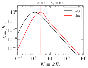
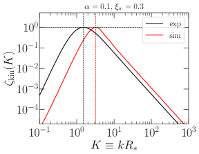
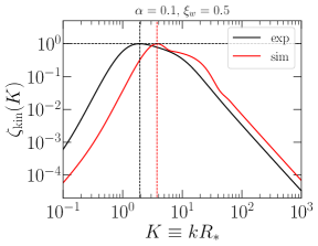
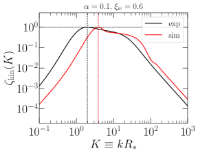
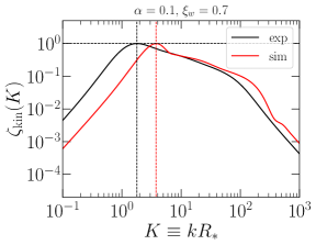
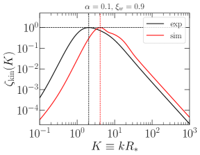
Figure 1: Time-independent component of the normalized velocity field UETC spectrum $\zeta_{\rm kin}(k)\equiv E_{\rm kin}(k)/E_{\rm kin}^{*}$ (see Eq. (39)), $E_{\rm kin}^{*}$ being the maximum value of the spectrum. Numerical results are obtained according to the sound shell model Hindmarsh and Hijazi (2019), as described in ref. Roper Pol et al. (2023b), for the phase transition strength parameter $\alpha=0.1$ and a range of wall velocities $\xi_{w}\in[0.1,0.9]$. The results are computed in the cases of exponential (black) and simultaneous (red) bubble nucleations Hindmarsh and Hijazi (2019). Vertical dashed lines indicate the wave numbers, $k_{\rm kin}^{\rm peak}$, where the maxima, $E_{\rm kin}^{*}$, are reached. Their numerical values are given in Table 1.

The functions ${\cal E}^{(n)}$ in Eq. (33) are

$${\cal E}^{(1)}(\chi)= \,|{\cal A}_{+}|^{2}=\frac{1}{4}\Bigl{[}{f^{\prime}}^{2}(\chi)+c_{\rm s}^{2}l^{2}(\chi)\Bigr{]},$$ (35)

$${\cal E}^{(2)}(\chi)= \,{\rm Re}\bigl{(}{\cal A}_{+}{\cal A}_{-}^{*}\bigr{)}=\frac{1}{4}\Bigl{[}{f^{\prime}}^{2}(\chi)-c_{\rm s}^{2}l^{2}(\chi)\Bigr{]},$$ (36)

$${\cal E}^{(3)}(\chi)= \,{\rm Im}\bigl{(}{\cal A}_{+}{\cal A}_{-}^{*}\bigr{)}=\frac{1}{2}c_{\rm s}f^{\prime}(\chi)\,l(\chi),$$ (37)

where ${\cal A}_{\pm}(\chi)$ are defined in Eq. (29).

Following ref. Hindmarsh and Hijazi (2019), we expect the amplitude of the oscillatory contributions corresponding to $E_{\rm kin}^{(1)}$ in Eq. (32) to be larger than those from $E_{\rm kin}^{(2)}$ and $E_{\rm kin}^{(3)}$. This is a consequence of the inequalities among their amplitudes,

$${\cal E}^{(1)}(\chi)\geq{\cal E}^{(2)}(\chi)\geq{\cal E}^{(3)}(\chi).$$ (38)

However, when the term proportional to $E_{\rm kin}^{(2)}$ is not highly oscillating, it cannot be neglected with respect to the one proportional to $E_{\rm kin}^{(1)}$. This occurs in the limit $\omega\equiv kc_{\rm s}\ll(2\delta\tau_{\rm fin})^{-1}$, since $0\leq\tau_{1}+\tau_{2}-2\tau_{*}\leq 2\delta\tau_{\rm fin}$, where we denote the duration of the source as $\delta\tau_{\rm fin}\equiv\tau_{\rm fin}-\tau_{*}$.

Let us first focus on the case $k\gg 1/(2c_{\rm s}\delta\tau_{\rm fin})$. Then, we find a stationary UETC Hindmarsh and Hijazi (2019),

$$E_{\rm kin}(k,\tau_{1},\tau_{2})\approx E_{\rm kin}(k)\cos(kc_{\rm s}\tau_{-})\,,$$ (39)

where $E_{\rm kin}(k)=E_{\rm kin}^{(1)}(k)$ and $\tau_{-}=\tau_{2}-\tau_{1}$. Figure (1) shows benchmark results for the normalized $\zeta_{\rm kin}(k)=E_{\rm kin}(k)/E_{\rm kin}^{*}$, $E_{\rm kin}^{*}$ denoting the maximum value of $E_{\rm kin}(k)$, obtained for a benchmark phase transition strength $\alpha=0.1$ and a range of broken-phase bubble wall speeds $\xi_{w}\in(0.1,0.9)$. We present the details of these calculations in an accompanying paper Roper Pol et al. (2023b).

Since the resulting velocity field due to the superposition of sound waves is irrotational, the causality condition requires $E_{\rm kin}(\tau_{1},\tau_{2},k)\sim k^{4}$ in the limit $k\rightarrow 0$ Monin and Yaglom (1975); Caprini et al. (2004); Hindmarsh and Hijazi (2019). We note that, since $E_{\rm kin}(k)$ is an integral over $\tilde{T}$ of ${\cal E}^{(1)}(\chi)$, the limit of $E_{\rm kin}(k)$ when $k\to 0$ is equivalent to the limit of ${\cal E}^{(1)}(\chi)$ when $\chi\to 0$. The integrand is then proportional to $f^{\prime 2}(\chi)+c_{\rm s}^{2}l^{2}(\chi)$, see Eq. (35).

As mentioned above, ref. Hindmarsh and Hijazi (2019) justifies the choice of $\lambda$ (which leads to the $c_{\rm s}^{2}l^{2}$ contribution in $E_{\rm kin}$) in Eq. (29) for the initial conditions, instead of $u^{\prime}$, to ensure the causality condition. However, the function $l^{2}(\chi)$ in Eq. (31) leads to the asymptotic limits $l^{2}(\chi)\sim\chi^{0}$ when $\chi\rightarrow 0$, and $E_{\rm kin}(k)\sim k^{2}$ when $k\to 0$, as we show in an accompanying paper Roper Pol et al. (2023b). This naively seems to violate causality. The same is true when one chooses $u^{\prime}$ to impose the initial conditions. The key point to recover the causality condition is to note that the assumption in Eq. (39) is not valid in the limit $k\ll 1/(2c_{\rm s}\delta\tau_{\rm fin})$. In this limit, one finds from Eq. (32),

$$\lim_{k\rightarrow 0}E_{\rm kin}(\tau_{1},\tau_{2},k)=E_{\rm kin}^{(1)}(k)+E_{\rm kin}^{(2)}(k).$$ (40)

The UETC of the velocity field in the $k\to 0$ limit is then proportional to ${f^{\prime}}^{2}(\chi)$ (see Eqs. (35) and (36)), and not to $l^{2}(\chi)$, as previously found using Eq. (39). Then the $\chi\to 0$ limit is indeed ${f^{\prime}}^{2}\sim\chi^{2}$, such that $E_{\rm kin}\sim k^{4}$, as expected from causality.

In the following, we take Eq. (39) to describe the UETC spectrum and will refer to $E_{\rm kin}$ as the kinetic spectrum. Even though $E_{\rm kin}$ does not describe the UETC in the limit $k\to 0$, it does for all the scales that are relevant for the study of GW production (see Fig. (1)).

type	$\xi_{w}$	$10^{4}E_{\rm kin}^{*}/R_{*}$	$K_{\rm kin}^{\rm peak}$	${\cal K}$	$10^{2}\Omega_{\rm K}$	${\cal C}$	$K_{\rm GW}$	$(K^{3}\zeta_{\Pi})_{\rm peak}$	$K_{1}$	$K_{2}$	$b$	$\alpha_{1}$	$\alpha_{2}$
exp	0.1	$26.8$	1.15	7.49	2.0	1.21	2.03	0.90	1.18	2.39	0.34	0.76	1.22
exp	0.2	$25.7$	1.28	5.42	1.4	0.94	2.39	1.36	1.59	2.39	1.06	0.66	1.33
exp	0.3	$21.6$	1.53	5.52	1.2	0.80	3.01	2.41	1.98	3.00	0	0.67	1.10
exp	0.4	$16.0$	1.80	8.43	1.4	0.76	4.01	4.93	1.99	6.70	0	0.70	1.30
exp	0.5	$10.3$	2.02	21.95	2.3	0.75	8.44	13.97	2.26	12.81	0.36	0.73	1.31
exp	0.6	$5.3$	2.28	58.88	3.1	0.75	20.33	68.80	2.79	26.94	0.78	0.68	1.08
exp	0.7	$3.2$	2.21	88.82	2.9	0.73	56.63	102.37	3.42	91.89	0.42	0.49	1.27
exp	0.8	$5.3$	2.05	22.98	1.2	0.72	9.53	14.09	1.63	11.94	1.47	1.81	0.39
exp	0.9	$5.1$	2.04	10.90	0.6	0.68	6.36	9.09	2.33	10.66	0	0.69	1.38
exp	0.99	$4.5$	2.04	7.95	0.4	0.66	4.99	7.36	2.20	7.82	0	0.73	1.49
sim	0.1	$18.2$	2.59	10.43	1.9	0.44	3.42	7.51	1.74	3.81	0.92	1.41	2.34
sim	0.2	$19.0$	2.82	7.08	1.3	0.31	4.03	10.85	2.09	4.04	0.93	1.34	2.13
sim	0.3	$16.1$	3.29	7.29	1.2	0.26	5.07	18.45	2.56	4.77	1.29	1.39	1.25
sim	0.4	$11.6$	3.64	11.11	1.3	0.25	6.76	35.29	3.53	10.50	0	0.92	2.39
sim	0.5	$7.2$	3.85	30.66	2.2	0.25	16.95	102.40	4.20	20.63	0.33	0.85	2.95
sim	0.6	$3.7$	4.16	84.35	3.1	0.25	40.79	528.01	5.36	44.62	0.75	0.71	2.15
sim	0.7	$2.3$	4.20	123.32	2.8	0.24	113.65	718.45	7.15	154.60	0.29	0.45	2.86
sim	0.8	$3.8$	4.06	31.14	1.2	0.23	16.07	97.56	3.14	23.38	1.02	1.70	0.71
sim	0.9	$3.6$	4.12	14.92	0.5	0.22	10.72	63.57	4.15	16.72	0	0.88	2.74
sim	0.99	$3.2$	4.13	10.84	0.4	0.22	8.41	52.26	3.96	12.37	0	0.96	2.66

Table 1: Numerical values of the amplitudes and peak frequencies that characterize the spectra of the velocity field (columns $3$ to $6$) and of GWs (columns $7$ to $9$), within the sound shell model for exponential and simultaneous types of nucleation Hindmarsh and Hijazi (2019); Roper Pol et al. (2023b). The bubble wall velocities $\xi_{w}$ correspond to the benchmark phase transitions shown in Fig. (1), with $\alpha=0.1$. The parameters in the last five columns determine the fit of $K^{3}\zeta_{\Pi}(K)$ in Eq. (50).

Following the normalization of ref. Roper Pol et al. (2022b), we define a characteristic amplitude $E_{\rm kin}^{*}$ and wave number $k_{*}$. For the kinetic spectrum corresponding to sound waves, we set $k_{*}=1/R_{*}$ and $E_{\rm kin}^{*}$ to be the maximum amplitude, which is located at $K_{\rm kin}^{\rm peak}=k_{\rm kin}^{\rm peak}R_{*}\sim{\cal O}(1)$ (see Fig. (1) and values in Table 1). Then, the kinetic spectrum can be expressed as

$$E_{\rm kin}(k)=E_{\rm kin}^{*}\,\zeta_{\rm kin}(K),$$ (41)

where $K=k/k_{*}=kR_{*}$ and $\zeta_{\rm kin}$ determines the spectral shape of the kinetic spectrum. The spectral shape found within the sound shell model (see Fig. (1)) is proportional to $k^{4}$ at low $k$, as discussed in Sec. (III.2), and follows a $k^{-2}$ decay at large $k$. At intermediate scales, $\zeta_{\rm kin}$ can present an additional intermediate power law, especially for values of the wall velocity $\xi_{w}$ close to the speed of sound $c_{\rm s}=1/\sqrt{3}$, and develop a double peak structure, as can be seen in Fig. (1) and shown in refs. Hindmarsh and Hijazi (2019); Gowling and Hindmarsh (2021).

The total kinetic energy density $\Omega_{\rm K}$, expressed as a fraction of the critical energy density, is computed from Eq. (39) at equal times $\tau_{1}=\tau_{2}=\tau$,

$$\Omega_{\rm K}=\int_{0}^{\infty}E_{\rm kin}(k,\tau,\tau){\rm\,d}k=\frac{E_{\rm kin}^{*}}{R_{*}}\,{\cal K},$$ (42)

where we have used Eq. (41), and

$${\cal K}\approx\int_{0}^{\infty}\zeta_{\rm kin}(K){\rm\,d}K,$$ (43)

only depends on the spectral shape, characterizing how broad is the spectrum around $K=1$. The values of ${\cal K}$ are listed in Table 1 for the benchmark phase transitions shown in Fig. (1). The kinetic energy density $\Omega_{\rm K}$ is estimated by the single-bubble profiles in ref. Espinosa et al. (2010) as $\Omega_{\rm K}\equiv\kappa\alpha/(1+\alpha)$, where $\kappa$ is an efficiency factor that depends on $\alpha$ and $\xi_{w}$. We omit the comparison of $\Omega_{\rm K}$ found in the sound shell model with that of ref. Espinosa et al. (2010) since we focus on the GW production in the current work. This relation will be explored in an accompanying paper Roper Pol et al. (2023b), see also the discussion of refs. Hindmarsh et al. (2014); Hindmarsh (2018); Hindmarsh et al. (2017); Hindmarsh and Hijazi (2019); Jinno et al. (2021, 2023).

III.3 UETC of the anisotropic stress

We consider the UETC of the anisotropic stresses $E_{\Pi}$, defined in Eq. (21), under the stationary assumption of Eq. (39). Introducing the normalization of Eqs. (41–43) one obtains

$$k\,E_{\Pi} (\tau_{1},\tau_{2},k)$$

$$\simeq 2\,\bar{w}^{2}\,K^{3}\,\biggl{(}\frac{\Omega_{\rm K}}{{\cal K}}\biggr{)}^{2}\,{\cal C}\,\zeta_{\Pi}(\tau_{-},K),$$ (44)

where, following ref. Roper Pol et al. (2022b), we have defined

$${\cal C}\,\zeta_{\Pi}(\tau_{-},K)= \,\int_{0}^{\infty}P^{2}\zeta_{\rm kin}(P)\,\cos(Pc_{\rm s}\,k_{*}\,\tau_{-})\,{\rm\,d}P$$

$$\int_{-1}^{1}(1-z^{2} )^{2}\,\frac{\zeta_{\rm kin}(\tilde{P})}{\tilde{P}^{4}}\cos(\tilde{P}c_{\rm s}\,k_{*}\,\tau_{-}){\rm\,d}z\,,$$ (45)

and used the notation $P\equiv p/k_{*}=pR_{*}$ and $\tilde{P}\equiv\tilde{p}/k_{*}=\tilde{p}R_{*}$. The constant ${\cal C}$ is the value of $\zeta_{\Pi}$ in the limit $K\to 0$ (see Table 1 for benchmark values),

$${\cal C}=\frac{16}{15}\int_{0}^{\infty}\frac{\zeta_{\rm kin}^{2}(K)}{K^{2}}{\rm\,d}K\,.$$ (46)

so that $\zeta_{\Pi}\to 1$ in this limit. The spectral shape is therefore encoded in $\zeta_{\Pi}$. We note that, as discussed in the previous section, the UETC of the velocity field in this limit should be taken from Eq. (40), so it does not only depend on the time difference $\tau_{-}$ when $k\ll 1/(2c_{\rm s}\delta\tau_{\rm fin})$.

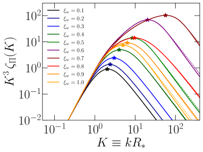
Figure 2: Normalized spectrum of the anisotropic stresses, $\zeta_{\Pi}$, for the kinetic spectra of the benchmark phase transitions shown in Fig. (1), in the case of exponential nucleation, computed numerically (solid lines) compared to the fit from Eq. (50) (dashed lines). $\zeta_{\Pi}$ is multiplied by $K^{3}$ since this is the relevant contribution to the resulting GW spectrum (see Sec. (VI)). The stars correspond to $K_{\rm GW}$, where $K^{3}\zeta_{\Pi}$ is maximum (see values in Table 1).

At equal times, Eq. (45) becomes

$${\cal C}\,\zeta_{\Pi}(K)=\int_{0}^{\infty} \,P^{2}\zeta_{\rm kin}(P){\rm\,d}P$$

$$\times\int_{-1}^{1}(1-z^{2})^{2}\,\frac{\zeta_{\rm kin}(\tilde{P})}{\tilde{P}^{4}}{\rm\,d}z,$$ (47)

where $\zeta_{\Pi}(K)\leq 1$ is a monotonically decreasing function, shown in Fig. (2) for the benchmark phase transitions of Fig. (1). This condition can be understood from the derivative of ${\cal C}\zeta_{\Pi}$ with respect to $K$,

$${\cal C}\,\partial_{K}\zeta_{\Pi} (K)=\int_{0}^{\infty}P^{2}\zeta_{\rm kin}(P){\rm\,d}P\int_{-1}^{1}(1-z^{2})^{2}\,$$

$$\times\biggl{[}\zeta_{\rm kin}^{\prime}(\tilde{P})-\frac{4\zeta_{\rm kin}(\tilde{P})}{\tilde{P}}\biggr{]}\frac{K-Pz}{\tilde{P}^{4}}{\rm\,d}z.$$ (48)

We find that the term in square brackets is always negative if $\zeta_{\rm kin}(\tilde{P})\propto\tilde{P}^{n}$ with $n\leq 4$ at all $\tilde{P}$, which is indeed the case. The second term $K-Pz$ is positive for most of the integration range since it becomes negative only when $z>K/P$. Since $1-z^{2}$ is symmetric in $z$, then the final integral is almost always negative, unless the term in the square bracket, once multiplied by $P^{2}\zeta_{\rm kin}(P)$, has a larger contribution when $K/P<1$ and $K/P<z<1$ than in the rest of the range, but this is not the case for any of the evaluated spectra (see Fig. (2)).

At intermediate $K$, $\zeta_{\Pi}$ strongly depends on the specific spectral shape of the velocity power spectrum $\zeta_{\rm kin}(K)$, and it requires numerical evaluation of the integral in Eq. (47). However, in the asymptotic limit $K\to\infty$, indicated by a $\infty$ superscript, Eq. (47) becomes

$$\zeta_{\Pi}^{\infty}=\frac{\zeta_{\rm kin}^{\infty}}{K^{4}}\frac{\displaystyle\int_{0}^{\infty}P^{2}\zeta_{\rm kin}(P){\rm\,d}P}{\displaystyle\int_{0}^{\infty}\frac{\zeta_{\rm kin}^{2}(P)}{P^{2}}{\rm\,d}P}\ .$$ (49)

Therefore, if the kinetic spectrum decays as $\zeta_{\rm kin}^{\infty}\sim K^{-b}$, then $\zeta_{\Pi}^{\infty}$ decays as $K^{-b-4}$. However, since $P$ is integrated from $0$ to $\infty$, it can become of the same order as $K$ and the power law decay $K^{-b-4}$ might not be reached exactly. In particular, we find $\zeta_{\Pi}^{\infty}\sim K^{-5}$, which is close to the estimated $K^{-6}$ slope, for the benchmark kinetic spectra (see Fig. (2), where dashed lines correspond to the fit in Eq. (50), with an exact $K^{-5}$ decay).

We find in Sec. (VI) that the final GW spectrum is proportional to $K^{3}\zeta_{\Pi}$ in the limit of short duration of the GW sourcing, $\delta\tau_{\rm fin}/R_{*}\ll 1$. For longer duration, the GW spectrum can deviate with respect to $K^{3}\zeta_{\Pi}$ by a factor $\tilde{\Delta}$ (see Sec. (VI)). In any case, the GW spectrum approximately peaks at $K_{\rm GW}$, defined as the wave number where $K^{3}\zeta_{\Pi}$ takes its maximum value $(K^{3}\zeta_{\Pi})_{\rm peak}$. The value of $K_{\rm GW}$ depends on how steep is the negative slope of $\zeta_{\Pi}$ when it starts to decay around $K\sim{\cal O}(1)$: it therefore requires numerical evaluation of $\zeta_{\Pi}$ using Eq. (47). We give in Table 1 the numerical values of $K_{\rm GW}$ and $(K^{3}\zeta_{\Pi})_{\rm peak}$.

Due to the double peak structure of $\zeta_{\rm kin}(K)$, which appears when the wall velocity $\xi_{w}$ approaches $c_{s}$, an appropriate fit for $K^{3}\zeta_{\Pi}$ is a smoothed doubly broken power law,

$$K^{3}\zeta_{\Pi}(K)=\frac{K^{3}\bigl{[}1+(K/K_{1})^{(3-b)\alpha_{1}}\bigr{]}^{-{1\over\alpha_{1}}}}{\bigl{[}1+(K/K_{2})^{(2+b)\alpha_{2}}\bigr{]}^{{1\over\alpha_{2}}}}\ ,$$ (50)

where $K_{1,2}$ are the wave number breaks, $b$ is the intermediate slope, and $\alpha_{1,2}$ are parameters that determine the smoothness of the transition between slopes. At low $K$, we fix $\zeta_{\Pi}=1$, as desired, and at large $K$, we fix $\zeta_{\Pi}^{\infty}\sim K^{-5}$. We note that, in general, $K_{2}$ is not necessarily equal to $K_{\rm GW}$. We show the corresponding values of $K_{1,2}$, $b$, and $\alpha_{1,2}$, found for the benchmark phase transitions of Fig. (1) in Table 1. We note that some $\zeta_{\Pi}$ are already well approximated by a single broken power law since they do not present a double peak structure, especially for $\xi_{w}\lesssim 0.5$ and $\xi_{w}\gtrsim 0.8$.

The exact values of the amplitude $(K^{3}\zeta_{\Pi})_{\rm peak}$, the frequency breaks $K_{1,2}$, and the intermediate slopes highly depend on the specific spectral shape of the velocity power spectrum $\zeta_{\rm kin}$. According to the sound shell model, refs. Hindmarsh (2018); Hindmarsh and Hijazi (2019) proposed that the two peaks are determined by the inverse mean size of the bubbles, $1/R_{*}$, and the inverse sound shell thickness, $1/(R_{*}\Delta_{w})$, where $\Delta_{w}=|\xi_{w}-c_{\rm s}|/c_{\rm s}$. Similar dependencies are found in numerical simulations Hindmarsh et al. (2014, 2015, 2017); Jinno et al. (2021, 2023). We explore the relations between the phase transition parameters and the shape of the anisotropic stresses, which will ultimately impact the GW spectrum, in an accompanying paper Roper Pol et al. (2023b). In the following, we study the spectral shape of GWs once we know the spectral shape of $\zeta_{\Pi}$, shown in Fig. (2) for a set of benchmark phase transitions.

IV Low wave number tail of the GW spectrum from sound waves

In this section, we study the amplitude of the GW spectrum analytically, by evaluating its low-frequency limit $k\to 0$. We do not assume flat space-time but consider an expanding Universe. Following the sound shell model Hindmarsh and Hijazi (2019), we adopt the stationary assumption of Eq. (39), assuming its validity down to $k\rightarrow 0$, see discussion in Sec. (III.2). The source is assumed to be stationary but still characterized by a finite lifetime, $\delta\tau_{\rm fin}$. Note that this might introduce a spurious effect in the final GW spectrum due to the sharp cutoff of the integrals in time Caprini et al. (2009b). However, we deem this not important, given the good agreement of the GW spectrum evaluated semi-analytically following the sound shell model with the one from numerical simulations Hindmarsh (2018); Hindmarsh and Hijazi (2019). The study of the GW spectrum at all $k$ is presented in Sec. (VI).

In Sec. (IV.1), we start by collecting the results of Sec. (III) to evaluate the GW spectrum, and comment on the consequences of the expansion of the Universe. We find in Sec. (IV.2) that the GW spectrum follows a $k^{3}$ scaling at low $k$: this is expected from previous analyses, both analytical Cai et al. (2023) and numerical Jinno et al. (2023); Sharma et al. (2023), but it is in contradiction with the findings of the original sound-shell model of ref. Hindmarsh and Hijazi (2019), which obtains instead that, at scales larger than the peak, the GW spectrum goes as $k^{9}$. In Sec. (IV.3), we reproduce the calculation of ref. Hindmarsh and Hijazi (2019) and show that the $k^{9}$ behavior is recovered only when one makes an assumption for the UETC that is, however, only justified under certain conditions that do not hold in the $k\to 0$ limit. We therefore claim that the $k^{3}$ scaling is the correct one in the low-$k$ limit.

Moreover, we find in Sec. (IV.2) that the GW amplitude in the $k\to 0$ limit is proportional to $\ln^{2}(1+\delta\tau_{\rm fin}{\cal H}_{*})$. This factor becomes quadratic in the source duration parameter $\delta\tau_{\rm fin}{\cal H}_{*}$ when one ignores the expansion of the Universe, i.e., in the limit $\delta\tau_{\rm fin}{\cal H}_{*}\ll 1$. A similar quadratic dependence has also been found in the numerical analysis of ref. Roper Pol et al. (2020b) for acoustic turbulence, as well as for (magneto)hydrodynamical ((M)HD) vortical turbulence, both analytically Caprini et al. (2009a, b); Roper Pol et al. (2022b) and numerically Roper Pol et al. (2020b); Kahniashvili et al. (2021); Brandenburg et al. (2021b, a); Roper Pol et al. (2022a, b); Auclair et al. (2022). However, this result is in contradiction with the linear dependence in the source duration usually assumed for stationary UETCs Kosowsky et al. (2002); Gogoberidze et al. (2007); Caprini et al. (2009a); Huber and Konstandin (2008b); Hindmarsh et al. (2014); Hindmarsh and Hijazi (2019); Guo et al. (2021). In particular, a linear growth is assumed for sound waves in analytical (see, e.g., refs. Caprini et al. (2016); Weir (2018); Caprini et al. (2020); Hindmarsh and Hijazi (2019); Hindmarsh et al. (2021); Gowling and Hindmarsh (2021); Gowling et al. (2023); Roper Pol et al. (2023a)) and numerical (see, e.g., refs. Hindmarsh et al. (2014, 2015, 2017); Cutting et al. (2020); Jinno et al. (2021, 2023)) studies. We investigate this issue in Sec. (V). We show that the linear growth of ref. Hindmarsh and Hijazi (2019), and the suppression factor $\Upsilon=1-1/(\tau_{\rm fin}{\cal H}_{*})$ of ref. Guo et al. (2021) for an expanding Universe, are valid for stationary processes only under specific assumptions Caprini et al. (2009a), which are equivalent to those used in refs. Hindmarsh and Hijazi (2019); Guo et al. (2021). We show that these assumptions do not hold in the $k\to 0$ limit. Therefore, the causality tail, proportional to $k^{3}$, is also proportional to $\ln^{2}(1+\delta\tau_{\rm fin}{\cal H}_{*})$.

In Sec. (V.2), we extend our analysis to a stationary Gaussian UETC (cf. Kraichnan decorrelation Kraichnan (1965); Kosowsky et al. (2002); Gogoberidze et al. (2007); Caprini et al. (2009b); Auclair et al. (2022)) to show, within a general framework, when the aforementioned assumptions hold. We find that this occurs when $k\tau_{c}\gg 1$, where $\tau_{c}$ is a characteristic time of the process (e.g., $\delta\tau_{\rm fin}$ in the sound shell model). Hence, if $\delta\tau_{\rm fin}/R_{*}\gg 1$, the slope of the GW spectrum around its spectral peak, $k_{\rm kin}^{\rm peak}\sim 1/R_{*}$, is well described under these assumptions. As discussed in Sec. (VI.2), this limit corresponds to low fluid velocities and correspondingly weak first-order phase transitions.

Indeed, in Sec. (VI), we extend our analysis to all $k$ and we show that, even though the causality tail is proportional to $k^{3}$ and follows a quadratic growth with $\delta\tau_{\rm fin}$, the amplitude around the peak can present a steep slope approaching the $k^{9}$ scaling, and can follow a linear growth with $\delta\tau_{\rm fin}$, when $\delta\tau_{\rm fin}/R_{*}\gg 1$. Hence, at frequencies $k\gg 1/\delta\tau_{\rm fin}$, the GW spectrum can be approximately described by the calculation of refs. Hindmarsh and Hijazi (2019); Guo et al. (2021), reproduced in App. (B). Including the expansion of the Universe, the quadratic $(\delta\tau_{\rm fin}\mathcal{H}_{*})^{2}$ and linear $\delta\tau_{\rm fin}\mathcal{H}_{*}$ dependence become respectively $\ln^{2}(1+\delta\tau_{\rm fin}{\cal H}_{*})$ and $\Upsilon$.

IV.1 GW spectrum in the sound shell model

We adopt the stationary assumption of Eq. (39) and combine Eqs. (15) and (21) to find the GW spectrum today. After averaging over fast oscillations in time, it becomes

$$\,\Omega_{\rm GW}(\delta\tau_{\rm fin},k)=3\,k^{3}\bar{w}^{2}\int_{-1}^{1}\bigl{(}1-z^{2}\bigr{)}^{2}\,{\rm\,d}z$$

$$\,\hskip 5.69054pt\times\int_{0}^{\infty}\!\!{\rm\,d}p\,\frac{p^{2}}{\tilde{p}^{4}}\,E_{\rm kin}(p)E_{\rm kin}(\tilde{p})\,\Delta(\delta\tau_{\rm fin},k,p,\tilde{p})\,.$$ (51)

Note that Eq. (51) gives the present-day GW spectrum, i.e., the observable we are generally interested in. While the source is still active, the GW spectrum would depend not only on the source duration $\delta\tau_{\rm fin}\equiv\tau_{\rm fin}-\tau_{*}$, but also on the absolute time $\tau$. During the production phase in the early Universe, in fact, the dependence on $\tau$ cannot be averaged out. We present this case in App. (A), which is particularly relevant when one compares it with the results of numerical simulations: depending on the wave number span and on the duration of the simulation, it is often required to take into account the residual dependence on $\tau$ of the GW spectrum, instead of on $\delta\tau_{\rm fin}$ only.

The function $\Delta$ in Eq. (51) contains the integral over times $\tau_{1}$ and $\tau_{2}$ of the Green’s functions and the time dependence of the stationary UETC,

$$\Delta(\delta\tau_{\rm fin}, \,k,p,\tilde{p})\equiv\int_{\tau_{*}}^{\tau_{\rm fin}}\!\!\frac{{\rm\,d}\tau_{1}}{\tau_{1}}\int_{\tau_{*}}^{\tau_{\rm fin}}\!\!\frac{{\rm\,d}\tau_{2}}{\tau_{2}}$$

$$\,\times\cos(pc_{\rm s}\tau_{-})\cos(\tilde{p}c_{\rm s}\tau_{-})\cos(k\tau_{-})\,.$$ (52)

The product of cosines can be expressed as

$$\cos(pc_{\rm s}\tau_{-})\cos(\tilde{p}c_{\rm s} \tau_{-})\cos(k\tau_{-})$$

$$\,=\frac{1}{4}\sum_{m,n=\pm 1}\cos(\hat{p}_{mn}\tau_{-})\,,$$ (53)

where we have defined $\hat{p}_{mn}\equiv(p+m\tilde{p})\,c_{\rm s}+nk$. We separate the time dependencies using

$$\cos(\hat{p}_{mn}\tau_{-})= \,\cos(\hat{p}_{mn}\tau_{2})\cos(\hat{p}_{mn}\tau_{1})$$

$$\,+\sin(\hat{p}_{mn}\tau_{2})\sin(\hat{p}_{mn}\tau_{1}),$$ (54)

so that the integrals over $\tau_{1}$ and $\tau_{2}$ yield

$$\Delta(\delta\tau_{\rm fin},k,p,\tilde{p})=\sum_{m,n=\pm 1}\Delta_{mn}(\delta\tau_{\rm fin},\hat{p}_{mn}),$$ (55)

where we have defined the function

$$\Delta_{mn} (\delta\tau_{\rm fin},\hat{p}_{mn})$$

$$= \,\frac{1}{4}\Bigl{[}\Delta{\rm Ci}^{2}(\tau_{\rm fin},\hat{p}_{mn})+\Delta{\rm Si}^{2}(\tau_{\rm fin},\hat{p}_{mn})\Bigr{]},$$ (56)

and

$$\Delta{\rm Ci}(\tau,p) \equiv{\rm Ci}\bigl{(}p\tau\bigr{)}-{\rm Ci}\bigl{(}p\tau_{*}\bigr{)}\,,$$ (57)

$$\Delta{\rm Si}(\tau,p) \equiv{\rm Si}\bigl{(}p\tau\bigr{)}-{\rm Si}\bigl{(}p\tau_{*}\bigr{)}\,.$$ (58)

Even though $\Delta_{mn}$ is an intermediate function, which needs to be integrated over $p$ and $z$ to obtain the GW spectrum (see Eq. (51)), it is still very useful to study its behavior as a function of both $\delta\tau_{\rm fin}{\cal H}_{*}$ and $\hat{p}_{mn}/{\cal H}_{*}$. In Fig. (3) we show $\Delta_{mn}$ as a function of $\delta\tau_{\rm fin}{\cal H}_{*}$ for different fixed values of $\hat{p}_{mn}/{\cal H}_{*}$.

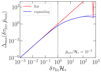
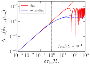
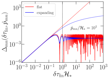
Figure 3: $\Delta_{mn}$ as a function of the duration of GW production $\delta\tau_{\rm fin}{\cal H}_{*}\equiv\tau_{\rm fin}{\cal H}_{*}-1$, given in units of the Hubble time $\tau_{*}={\cal H}_{*}^{-1}$, for an expanding (blue, Eq. (56)), and a flat (red, Eq. (59)) Universe. The four panels show different values of the combined momenta $\hat{p}_{mn}/{\cal H}_{*}\in\{10^{-2},10^{-1},1,10\}$. The dashed lines correspond to the asymptotic limits: $(\delta\tau_{\rm fin}{\cal H}_{*})^{2}$ when $\delta\tau_{\rm fin}{\cal H}_{*}\ll 1$ (red), and $\ln^{2}(\tau_{\rm fin}{\cal H}_{*})$ when $\hat{p}_{mn}\ll{\cal H}_{*}$ for an expanding Universe (blue). Both asymptotic limits are equivalent when $\delta\tau_{\rm fin}{\cal H}_{*}\ll 1$.

In the limit $\hat{p}_{mn}\ll{\cal H}_{*}$, the functions $\Delta{\rm Ci}\rightarrow\ln(\tau_{\rm fin}{\cal H}_{*})$ and $\Delta{\rm Si}\rightarrow 0$, such that $\Delta\rightarrow\ln^{2}(\tau_{\rm fin}{\cal H}_{*})=\ln^{2}(1+\delta\tau_{\rm fin}{\cal H}_{*})$ (see Fig. (3)). This limit is very relevant: we show in Sec. (IV.2) that, indeed, this logarithmic scaling with the source duration holds also for the GW spectrum in the $k\to 0$ limit.

If the duration of the production of GWs from sound waves is short, $\delta\tau_{\rm fin}{\cal H}_{*}\ll 1$, the expansion of the Universe can be neglected. As a consequence, $\tau\approx 1/{\cal H}_{*}$ in Eq. (4), and the factor $1/(\tau_{1}\tau_{2})$ in the integrand of Eq. (52) becomes constant, ${\cal H}_{*}^{2}$. In this case, we obtain the solution for a flat (non-expanding) Universe,

$$\Delta_{mn}^{\rm flat}(\delta\tau_{\rm fin}, \,\hat{p}_{mn})=$$

$$\frac{1-\cos\bigl{[}(\hat{p}_{mn}/{\cal H}_{*})({\cal H}_{*}\delta\tau_{\rm fin})\bigr{]}}{2\,\bigl{(}\hat{p}_{mn}/{\cal H}_{*}\bigr{)}^{2}}\ .$$ (59)

Since $\delta\tau_{\rm fin}{\cal H}_{*}\ll 1$, one has $\Delta^{\rm flat}\rightarrow(\delta\tau_{\rm fin}{\cal H}_{*})^{2}$ from Eq. (59), suggesting that the GW spectrum grows quadratically in $\delta\tau_{\rm fin}$. This quadratic scaling also holds for an expanding Universe, since the same limit can be found from Eq. (56): for $\hat{p}_{mn}\ll{\cal H}_{*}$ and $\delta\tau_{\rm fin}{\cal H}_{*}\ll 1$, one has $\Delta\to\ln^{2}(1+\delta\tau_{\rm fin}{\cal H}_{*})\rightarrow(\delta\tau_{\rm fin}{\cal H}_{*})^{2}$. These behaviors for a flat and an expanding Universe are shown in Fig. (3) and are due to the asymptotic limits of the cosine and sine integral functions, as pointed out in refs. Caprini et al. (2009a); Roper Pol et al. (2022b).

IV.2 Low-frequency limit

In the previous section, we have shown that the function $\Delta_{mn}$, given in Eqs. (56) and (59) respectively for an expanding and a flat Universe, depends logarithmically on the duration of the source, $\ln^{2}(\tau_{\rm fin}{\cal H}_{*})$, for small values of $\hat{p}_{mn}/{\cal H}_{*}$. In this section, we compute explicitly the GW spectrum in the limit $k\to 0$, and confirm that the GW spectrum inherits the same logarithmic dependence at large scales. We also show how the $k^{3}$ scaling, expected from causality Caprini et al. (2004), appears in this limit, instead of the $k^{9}$ scaling found in ref. Hindmarsh and Hijazi (2019).

In the low frequency limit $k\to 0$, $\tilde{p}\to p$ and $\hat{p}_{mn}\rightarrow(p+m\tilde{p})\,c_{\rm s}$. The latter becomes $0$ for $m=-1$ and $2pc_{\rm s}$ for $m=1$. Therefore, the $z$-dependence in Eq. (51) is reduced only to the function $(1-z^{2})^{2}$, and the GW spectrum becomes

$$\lim_{k\rightarrow 0} \,\Omega_{\rm GW}(\delta\tau_{\rm fin},k)=$$

$$\,3\,\bar{w}^{2}\,k^{3}\,\frac{16}{15}\int_{0}^{\infty}\frac{E_{\rm kin}^{2}(p)}{p^{2}}\Delta_{0}(\delta\tau_{\rm fin},p){\rm\,d}p.$$ (60)

This expression already shows an important result: the GW spectrum scales with $k^{3}$ in the limit $k\rightarrow 0$, since the integral in Eq. (60) does not depend on $k$. We defer the comparison of this result to the $k^{9}$ scaling found in ref. Hindmarsh and Hijazi (2019) to Sec. (IV.3). There, we demonstrate that a simplifying approximation of $\Delta$ used in ref. Hindmarsh and Hijazi (2019) leads to an additional dependence of $\Delta_{0}$ on $k$. However, this approximation does not apply in the $k\to 0$ limit, invalidating the $k^{9}$ behaviour at large scales. In the following, we rather focus on the dependence of $\Omega_{\rm GW}$ with the source duration $\delta\tau_{\rm fin}$.

The $\Delta_{0}$ function that appears in Eq. (60) corresponds to $\Delta$, given in Eq. (55), in the $k\to 0$ limit:

$$\Delta_{0}(\delta\tau_{\rm fin},p)=\lim_{k\rightarrow 0}\Delta(\delta\tau_{\rm fin},k, \,p,\tilde{p})$$

$$=\frac{1}{2}\Bigl{[}\ln^{2}(\tau_{\rm fin}{\cal H}_{*})+ \,\Delta{\rm Ci}^{2}(\tau_{\rm fin},2pc_{\rm s})$$

$$+ \,\Delta{\rm Si}^{2}(\tau_{\rm fin},2pc_{\rm s})\Bigr{]},$$ (61)

which, for a flat (non-expanding) Universe, reduces to

$$\Delta_{0}^{\rm flat}(\delta\tau_{\rm fin},p)= \,\lim_{k\rightarrow 0}\Delta^{\rm flat}(\delta\tau_{\rm fin},k,p,\tilde{p})$$

$$=\frac{1}{2}\Biggl{[} \,\bigl{(}\delta\tau_{\rm fin}{\cal H}_{*}\bigr{)}^{2}+\frac{\sin^{2}\bigl{(}pc_{\rm s}\delta\tau_{\rm fin}\bigr{)}}{\bigl{(}pc_{\rm s}/{\cal H}_{*}\bigr{)}^{2}}\Biggr{]}.$$ (62)

We find in Eq. (61) a first term, ${\textstyle{1\over 2}}\ln^{2}(\tau_{\rm fin}{\cal H}_{*})$, independent of $p$, and a second term that depends on $p$ and will enter the integral over $p$ in Eq. (60). We can parameterize the dependence of the GW amplitude with $\delta\tau_{\rm fin}$ by defining a weighted average of the function $\Delta_{0}$ with the spectral function $\zeta_{\rm kin}$,

$$\tilde{\Delta}_{0}(\delta\tau_{\rm fin}, \,R_{*})$$

$$= \,\frac{\displaystyle\int_{0}^{\infty}\frac{\zeta_{\rm kin}^{2}(K)}{K^{2}}\,\Delta_{0}(\delta\tau_{\rm fin},K/R_{*})\,{\rm\,d}K}{\displaystyle\int_{0}^{\infty}\frac{\zeta_{\rm kin}^{2}(K)}{K^{2}}{\rm\,d}K}\ ,$$ (63)

where we have used the normalized quantities $\zeta_{\rm kin}(K)=E_{\rm kin}(K)/E_{\rm kin}^{*}$ and $K\equiv k/k_{*}=kR_{*}$, defined in Sec. (III.3). Introducing Eq. (63) into Eq. (60), and using the normalization of Sec. (III.3) for the UETC of the anisotropic stresses, we find

$$\lim_{K\rightarrow 0}\Omega_{\rm GW} (\delta\tau_{\rm fin},K)$$

$$= \,3\,\bar{w}^{2}\,K^{3}\biggl{(}\frac{\Omega_{\rm K}}{{\cal K}}\biggr{)}^{2}\,{\cal C}\,\tilde{\Delta}_{0}(\delta\tau_{\rm fin},R_{*}),$$ (64)

where $E_{\rm kin}^{*}=\Omega_{\rm K}R_{*}/{\cal K}$, see Eq. (42). Since the dimensionless kinetic power spectrum $\zeta_{\rm kin}$ is peaked at $K_{\rm kin}^{\rm peak}=k_{\rm kin}^{\rm peak}R_{*}\sim{\cal O}(1)$ (see Fig. (1)), we can approximate it as $\zeta_{\rm kin}(K)\sim\delta(K-1)$ in the integrals of Eq. (63). Under this assumption, $\tilde{\Delta}_{0}(\delta\tau_{\rm fin})\to\Delta_{0}(\delta\tau_{\rm fin},1)$, showing that $\tilde{\Delta}_{0}/\Delta_{0}$ characterizes the deviations with respect to a delta-peaked kinetic power spectrum. We can now study the dependence of $\tilde{\Delta}_{0}$ with $\delta\tau_{\rm fin}$ under this approximation,

$$\tilde{\Delta}_{0} (\delta\tau_{\rm fin},\,R_{*})\sim\frac{1}{2}\Biggl{\{}\ln^{2}(\tau_{\rm fin}{\cal H}_{*})\,+$$ (65)

$$\left[{\rm Ci}\left(\frac{2c_{s}}{\mathcal{H}_{*}R_{*}}+2c_{s}\frac{\delta\tau_{\rm fin}}{R_{*}}\right)-{\rm Ci}\left(\frac{2c_{s}}{\mathcal{H}_{*}R_{*}}\right)\right]^{2}+$$

$$\left[{\rm Si}\left(\frac{2c_{s}}{\mathcal{H}_{*}R_{*}}+2c_{s}\frac{\delta\tau_{\rm fin}}{R_{*}}\right)-{\rm Si}\left(\frac{2c_{s}}{\mathcal{H}_{*}R_{*}}\right)\right]^{2}\Biggr{\}}\,.$$

If $c_{s}\delta\tau_{\rm fin}/R_{*}\ll 1$, from the expansion of the ${\rm Ci}$ and ${\rm Si}$ functions one gets:

$$\tilde{\Delta}_{0}(c_{s}\delta\tau_{\rm fin}/R_{*}\ll 1) \sim\frac{1}{2}\left\{\ln^{2}(\tau_{\rm fin}{\cal H}_{*})+(\delta\tau_{\rm fin}\mathcal{H}_{*})^{2}\right\}$$

$$\sim(\delta\tau_{\rm fin}\mathcal{H}_{*})^{2}\,,$$ (66)

where the last estimate holds when $\delta\tau_{\rm fin}{\cal H}_{*}\ll R_{*}{\cal H}_{*}\leq 1$. In the opposite limit $c_{s}\delta\tau_{\rm fin}/R_{*}\gg 1$, the contribution from the ${\rm Ci}$ and ${\rm Si}$ functions is oscillating and decaying, and therefore subdominant. One expects therefore:

$$\tilde{\Delta}_{0}(c_{s}\delta\tau_{\rm fin}/R_{*}\gg 1) \sim\frac{1}{2}\ln^{2}(\tau_{\rm fin}{\cal H}_{*})\,.$$ (67)

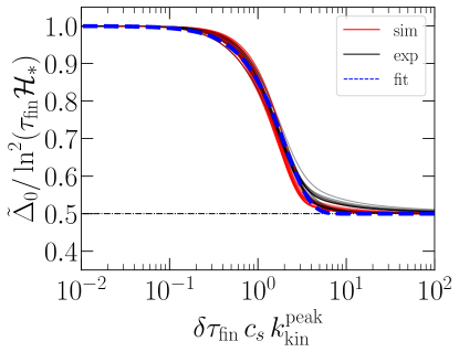
Figure 4: The function $\tilde{\Delta}_{0}$ compensated by its short-duration limit $\ln^{2}(\tau_{\rm fin}{\cal H}_{*})$. $\tilde{\Delta}_{0}$ is shown as a function of $\delta\tau_{\rm fin}\,c_{\rm s}\,k_{\rm kin}^{\rm peak}$, where $k_{\rm kin}^{\rm peak}\sim{\cal O}(1/R_{*})$ is the spectral peak of the kinetic spectra shown in Fig. (1), see dashed lines and values in Table 1. The blue dashed line corresponds to the empirical fit in Eq. (68).

The asymptotic behavior at the extremes of the quantity $c_{s}\delta\tau_{\rm fin}R_{*}$ is confirmed by Fig. (4), showing the function $\tilde{\Delta}_{0}$, compensated by the logarithmic dependence $\ln^{2}(\tau_{\rm fin}{\cal H}_{*})$, for the benchmark phase transitions of Fig. (1). One can appreciate that almost all curves collapse into one, apart from small deviations, which are due to the specific spectral shape of the kinetic spectra $\zeta_{\rm kin}(k)$ around their peak $k_{\rm kin}^{\rm peak}$, see Fig. (1). In all the cases considered, the dependence of the GW amplitude with $\delta\tau_{\rm fin}$ given in Eq. (64) can be expressed as $A\ln^{2}(\tau_{\rm fin}{\cal H}_{*})$, where $A$ monotonically decreases around $\delta\tau_{\rm fin}\sim(c_{\rm s}k_{\rm kin}^{\rm peak})^{-1}$ between its asymptotic values, i.e., from 1 to 0.5, as it can be derived approximately from Eqs. (65–67). The exact variation of the function $A$ at intermediate $\delta\tau_{\rm fin}$ requires numerical computation of Eq. (63) for the specific spectral shape $\zeta_{\rm kin}$. However, we show in Fig. (4) that the empirical fit

$$A\approx\frac{1}{2}\biggl{[}1+\exp\Bigl{(}-0.35\,\bigl{[}\delta\tau_{\rm fin}\,c_{\rm s}\,k_{\rm kin}^{\rm peak}\bigr{]}^{1.5}\Bigr{)}\biggr{]},$$ (68)

gives an accurate estimate for the evaluated phase transitions.

By taking the low-frequency limit $k\to 0$ of the GW spectrum, we have found that its amplitude depends quadratically on the duration of the GW source when $\delta\tau_{\rm fin}$ is short, compared to the Hubble time, and it is proportional to $\ln^{2}(\tau_{\rm fin}{\cal H}_{*})$ in general (see Fig. (4)). As previously discussed, this result is in contradiction with the linear dependence on the source duration usually assumed for the GW spectrum from sound waves, and from stationary processes in general. We come back to this aspect in Sec. (V) and extend the discussion to a generic class of stationary UETC. In the next Sec. (IV.3), we instead analyze the $k$-dependence of the GW spectrum at large scales, and provide insight on the reasons why a $k^{9}$ behavior is found in refs. Hindmarsh and Hijazi (2019); Guo et al. (2021), as opposed to the usual causal $k^{3}$ scaling given in Eq. (64).

IV.3 $k^{3}$ vs $k^{9}$ tilt in the low-frequency limit

In Sec. (IV.2), we have found that the GW spectrum scales proportional to $k^{3}$ when $k\rightarrow 0$ (see Eq. (64)). The causal $k^{3}$ branch is, in general, in agreement with numerical simulations of sound waves Hindmarsh et al. (2014, 2015); Jinno et al. (2021, 2023); Sharma et al. (2023) and the recent analytical derivation of ref. Cai et al. (2023). However, as mentioned above, it is in contradiction with the $k^{9}$ scaling reported in the sound shell model Hindmarsh (2018); Hindmarsh and Hijazi (2019); Guo et al. (2021). To understand the $k^{3}$ vs $k^{9}$ discrepancy of the GW spectrum, we reproduce in this section the calculation of refs. Hindmarsh and Hijazi (2019); Guo et al. (2021). Since ref. Hindmarsh and Hijazi (2019) considers that the duration of the phase transition is short and hence ignores the expansion of the Universe, we will consider the limit $\delta\tau_{\rm fin}{\cal H}_{*}\ll 1$ when comparing our results to theirs.

In order to reproduce the calculations of ref. Hindmarsh and Hijazi (2019), we need to compute the growth rate of $\Omega_{\rm GW}$ with the duration of GW production, $\delta\tau_{\rm fin}$. Note that in ref. Hindmarsh and Hijazi (2019), the growth rate $\dot{\Delta}$ [see their Eq.(3.38)] is defined instead as the derivative of $\Delta$ with respect to cosmic time $t$. We consider this interpretation to be misleading since $\Delta$, see Eq. (52), has been defined after averaging over time and it is valid only in the free propagation regime at late times $\tau\gg\tau_{\rm fin}$, e.g., at present time $\tau_{0}$ (see Eqs. (12) and (15)). We show in App. (A) the correct time-dependence of $\Delta$ with conformal time during the phase of GW production, $\tau<\tau_{\rm fin}$. We note that using Eq. (55) during the sourcing could lead to wrong results when comparing, for example, to the results from numerical simulations Hindmarsh et al. (2014, 2015, 2017); Jinno et al. (2021, 2023).

As a present-day observable, we are then interested in the dependence of the GW spectrum with the source duration $\delta\tau_{\rm fin}$, so we define $\Delta^{\prime}\equiv\partial_{\tau_{\rm fin}}\Delta$. Note that in the current work, we distinguish $\Delta^{\prime}$ from $\dot{\Delta}\equiv\partial_{t_{\rm fin}}\Delta$ since we take into account the expansion of the Universe.

We start by performing the change of variables $\{\tau_{1,2}\}\to\{\tau_{\pm}\}$ in the integral of Eq. (52), with $\tau_{+}\equiv(\tau_{1}+\tau_{2})/2$ and $\tau_{-}\equiv\tau_{2}-\tau_{1}$. The limits of integration can be found in the following way. Since $\tau_{1},\tau_{2}\in[\tau_{*},\tau_{\rm fin}]$, one has that $\tau_{+}\in[\tau_{*},\tau_{\rm fin}]$, and

$$\tau_{-}=2(\tau_{+}-\tau_{1})=2(\tau_{2}-\tau_{+}),$$ (69)

which, since $\tau_{1},\tau_{2}\in[\tau_{*},\tau_{\rm fin}]$, leads to the limits

$$\tau_{-}\in 2\ [-\delta\tau_{+}^{\rm fin},\delta\tau_{+}]\;\vee\;\tau_{-}\in 2\ [-\delta\tau_{+},\delta\tau_{+}^{\rm fin}],$$ (70)

where we have defined $\delta\tau_{+}\equiv\tau_{+}-\tau_{*}$ and $\delta\tau_{+}^{\rm fin}\equiv\tau_{\rm fin}-\tau_{+}$. Combining both limits we see that, when $\tau_{+}\leq\tau_{m}\equiv{\textstyle{1\over 2}}(\tau_{*}+\tau_{\rm fin})$, the limits of integration for $\tau_{-}$ are $\tau_{-}\in 2\,[-\delta\tau_{+},\delta\tau_{+}]$, and when $\tau_{+}>\tau_{m}$, then $\tau_{-}\in 2\,[-\delta\tau_{+}^{\rm fin},\delta\tau_{+}^{\rm fin}]$; see Fig. (5). Hence, the change of variables $\{\tau_{1,2}\}\to\{\tau_{\pm}\}$ in Eq. (52) yields

$$\Delta_{mn}(\delta \tau_{\rm fin},\hat{p}_{mn})=\int_{\tau_{*}}^{\tau_{\rm fin}}\!\!\frac{{\rm\,d}\tau_{1}}{2\tau_{1}}\int_{\tau_{*}}^{\tau_{\rm fin}}\!\!\frac{{\rm\,d}\tau_{2}}{2\tau_{2}}\cos(\hat{p}_{mn}\tau_{-})$$

$$= \,\int_{\tau_{*}}^{\tau_{m}}{\rm\,d}\tau_{+}\int_{-2\delta\tau_{+}}^{2\delta\tau_{+}}\frac{\cos(\hat{p}_{mn}\tau_{-})}{4\tau_{+}^{2}-\tau_{-}^{2}}{\rm\,d}\tau_{-}$$

$$+ \,\int_{\tau_{m}}^{\tau_{\rm fin}}{\rm\,d}\tau_{+}\int_{-2\delta\tau_{+}^{\rm fin}}^{2\delta\tau_{+}^{\rm fin}}\frac{\cos(\hat{p}_{mn}\tau_{-})}{4\tau_{+}^{2}-\tau_{-}^{2}}{\rm\,d}\tau_{-}\ .$$ (71)

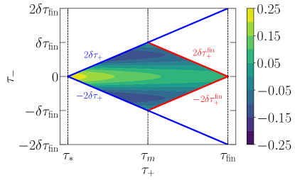
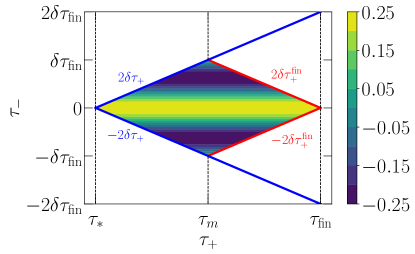
Figure 5: The limits of integration for the change of variables $\{\tau_{1,2}\}\to\{\tau_{\pm}\}$, with $\tau_{+}\equiv(\tau_{1}+\tau_{2})/2$ and $\tau_{-}\equiv\tau_{2}-\tau_{1}$ in the $\tau_{1,2}\in[\tau_{*},\tau_{\rm fin}]$ range corresponds to the region bounded by the blue and red lines. The extension of the blue lines up to $\tau_{\rm fin}$ indicates the region considered for the same integration in ref. Hindmarsh and Hijazi (2019), which thus ignores the bounds given by the red lines. For illustration, we show contour values of the integrand multiplied by ${\cal H}_{*}^{2}$ for an expanding (Eq. (71), upper panel) and a flat (Eq. (72), lower panel) Universe, with $\hat{p}_{mn}/{\cal H}_{*}=5$.

In particular, if we ignore the expansion of the Universe, we can set $\tau_{*}\to 0$ and take $\tau_{1}\tau_{2}\approx 1/{\cal H}_{*}^{2}$ in Eq. (71), such that $\Delta_{mn}$ becomes

$$4\,\Delta_{mn}^{\rm flat} (\delta\tau_{\rm fin},\hat{p}_{mn})=$$

$$\,{\cal H}_{*}^{2}\int_{0}^{{\textstyle{1\over 2}}\tau_{\rm fin}}{\rm\,d}\tau_{+}\int_{-2\tau_{+}}^{2\tau_{+}}\cos(\hat{p}_{mn}\tau_{-}){\rm\,d}\tau_{-}$$

$$+ \,{\cal H}_{*}^{2}\int_{{\textstyle{1\over 2}}\tau_{\rm fin}}^{\tau_{\rm fin}}{\rm\,d}\tau_{+}\int_{-2\delta\tau_{+}^{\rm fin}}^{2\delta\tau_{+}^{\rm fin}}\cos(\hat{p}_{mn}\tau_{-}){\rm\,d}\tau_{-}.$$ (72)

Figure (5) shows the values of the integrand in Eqs. (71) and (72) as a function of $\tau_{\pm}$. Ignoring the expansion of the Universe, the integrand is constant in $\tau_{+}$ and only depends on $\tau_{-}$ as $\cos(\hat{p}_{mn}\tau_{-})$.

If we compare this integral with the one computed in ref. Hindmarsh and Hijazi (2019) (see their Eq. (3.36)), we find that the limits of the integral are taken to be $\tau_{+}\in[0,\tau_{\rm fin}]$ and $\tau_{-}\in[-2\tau_{+},2\tau_{+}]$. This corresponds to integrating over $\tau_{-}$ according to the blue limits in Fig. (5) in all the range $\tau_{+}\in[0,\tau_{\rm fin}]$, hence including the areas of integration that are not allowed, limited by the red lines. The inclusion of the upper and lower right triangles, out of the limits denoted by the red lines, leads to $\tau_{2}>\tau_{\rm fin}$ and $\tau_{1}>\tau_{\rm fin}$, respectively. Using these limits of integration, the explicit dependence of the limits of the integral over $\tau_{-}$ on the source duration $\tau_{\rm fin}$ is ignored, leading to the wrong value of $\Delta^{\prime}$, as we show below.

We now compute the growth rate $\Delta^{\prime}$ from Eq. (71),

$$\Delta^{\prime}_{mn}(\delta\tau_{\rm fin},\hat{p}_{mn})$$

$$=\frac{1}{2\,\tau_{\rm fin}}\Bigl{[} \,\cos\bigl{(}\hat{p}_{mn}\tau_{\rm fin}\bigr{)}\Delta{\rm Ci}(\tau_{\rm fin},\hat{p}_{mn})$$

$$+ \,\sin\bigl{(}\hat{p}_{mn}\tau_{\rm fin}\bigr{)}\Delta{\rm Si}(\tau_{\rm fin},\hat{p}_{mn})\Bigr{]}\ ,$$ (73)

which can also be directly found from Eq. (56). Ignoring the expansion of the Universe we get, from either Eq. (59) or Eq. (72),

$$\Delta_{mn}^{\rm flat^{\prime}}(\delta\tau_{\rm fin},\hat{p}_{mn})={\cal H}_{*}\,\frac{\sin\bigl{(}\hat{p}_{mn}\delta\tau_{\rm fin}\bigr{)}}{2\,(\hat{p}_{mn}/{\cal H}_{*})}.$$ (74)

If one omits the dependence on $\tau_{\rm fin}$ in the integration limits over $\tau_{-}$ in Eq. (72), the solution to Eq. (3.38) of ref. Hindmarsh and Hijazi (2019) is found, which is equivalent to Eq. (74) with an extra factor 2 in the $\sin$ function, $\sin(2\hat{p}_{mn}\delta\tau_{\rm fin})$.

Figure (6) shows the dependence of the growth rate $\Delta^{\prime}_{mn}$, given in Eqs. (73) and (74), on the combined momenta $\hat{p}_{mn}$ for different values of the GW source duration $\delta\tau_{\rm fin}$. We observe that, as $\delta\tau_{\rm fin}$ increases, $\Delta^{\prime}_{mn}$ becomes more confined around $\hat{p}_{mn}\rightarrow 0$. Taking into account the relation between the sinc and the Dirac $\delta$ function,

$$\delta(x)=\lim_{a\to 0}\frac{\sin(\pi x/a)}{\pi x},$$ (75)

ref. Hindmarsh and Hijazi (2019) approximates Eq. (74) in the $1/\delta\tau_{\rm fin}\to 0$ limit, i.e., for large GW duration,

$$\lim_{\delta\tau_{\rm fin}{\cal H}_{*}\to\infty}\Delta_{mn}^{\rm flat^{\prime}}(\hat{p}_{mn})={\cal H}_{*}\frac{\pi}{2}\delta\bigl{(}\hat{p}_{mn}/{\cal H}_{*}\bigr{)}.$$ (76)

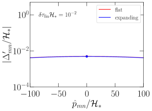
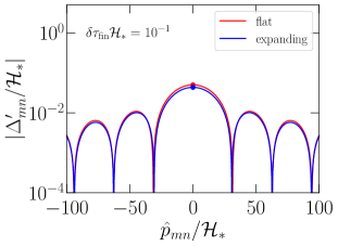
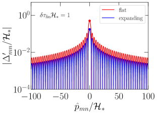
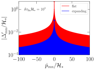
Figure 6: Function $|\Delta^{\prime}_{mn}|/{\cal H}_{*}$ for an expanding (blue, Eq. (73)) and a flat (red, Eq. (74)) Universe as a function of $\hat{p}_{mn}/{\cal H}_{*}$ for different GW sourcing duration $\delta\tau_{\rm fin}{\cal H}_{*}\in\{10^{-2},10^{-1},1,10\}$.

This approximation is used in refs. Hindmarsh and Hijazi (2019); Guo et al. (2021) to simplify the calculation of the integral in Eq. (51). However, it is not required to compute the GW amplitude, as we have done in Sec. (IV.2) in the $k\to 0$ limit and we extend in Sec. (VI) to all $k$. We show in the following that it is precisely this assumption the one that leads to the linear growth with the source duration and the $k^{9}$ scaling of the GW spectrum when $k\to 0$. We also show in Sec. (V) that this assumption is equivalent to the one usually taken for stationary processes that decay very quickly with the time difference $\tau_{-}$ Kraichnan (1965); Kosowsky et al. (2002); Gogoberidze et al. (2007); Caprini et al. (2009a, b); Niksa et al. (2018); Auclair et al. (2022). However, the UETC found in the sound shell model is a periodic function in $\tau_{-}$ (see Eq. (39)) so this assumption is, in general, not justified.

On the other hand, when $k$ is large and oscillations over $\tau_{-}$ become very rapid, this assumption might become justified. In such circumstances, as we show in Sec. (VI), the expression computed in App. (B), based on this approximation, can describe the GW spectrum in the regime $k\gg 1/\delta\tau_{\rm fin}$ and, in particular, around the spectral peak if $\delta\tau_{\rm fin}/R_{*}\gg 1$. One can understand this by noting that the limit leading to Eq. (76) is equivalent to considering $\hat{p}_{mn}\delta\tau_{\rm fin}\to\infty$. At low and moderate $k$, in general, this limit does not hold, since $p$ and $\tilde{p}$ are integrated from 0 to $\infty$. However, when $k\delta\tau_{\rm fin}\to\infty$, this assumption is valid, since $\Delta_{mn}$ is symmetric in $\hat{p}_{mn}$ and then $\hat{p}_{mn}\delta\tau_{\rm fin}\to\infty$.

We note that this approximation is only valid when $k\delta\tau_{\rm fin}$ becomes sufficiently large, not when $\tau$ is large, since $\Delta^{\prime}$ is the growth with respect to $\delta\tau_{\rm fin}$. The assumption of asymptotically large $\delta\tau_{\rm fin}$ is not justified for GW production from sound waves and it is in contradiction with the assumption that the expansion of the Universe can be ignored, so expansion becomes relevant in this regime.

In general, we find that $\Delta^{\prime}_{mn}$ is widely spread along a broad range of $\hat{p}_{mn}\neq 0$ for short and moderate (around one Hubble time) duration (see Fig. (6)). Its maximum value at $\hat{p}_{mn}=0$ is ${\textstyle{1\over 2}}\,\delta\tau_{\rm fin}{\cal H}_{*}$, as can be inferred from Eq. (74). For longer sourcing duration, one can no longer ignore the expansion of the Universe and we find that the growth rate at $\hat{p}_{mn}=0$ decreases to ${\textstyle{1\over 2}}\,\ln(\tau_{\rm fin}{\cal H}_{*})/\tau_{\rm fin}$ (see blue and red dots in Fig. (6)). Therefore, the integral over $p$ and $z$ in Eq. (51) includes non-negligible contributions from $\hat{p}_{mn}\neq 0$ that are being ignored if one uses Eq. (76).

We now explicitly show how this approximation affects the limit $k\to 0$ of the GW spectrum, computed in Sec. (IV.2). Denoting $\Omega_{\rm GW}^{\prime}\equiv\partial_{\tau_{\rm fin}}\Omega_{\rm GW}$ as the growth rate of the GW spectrum and using Eqs. (64) and (76), we find,

$$\lim_{K\rightarrow 0}\Omega_{\rm GW}^{\prime} (\delta\tau_{\rm fin},K)=\frac{8\pi}{5}\,R_{*}\,\bar{w}^{2}\,K^{3}\,\biggl{(}\frac{\Omega_{\rm K}}{\cal K}\biggr{)}^{2}$$

$$\times \,\int_{0}^{\infty}\frac{\zeta_{\rm kin}^{2}(P)}{P^{2}}\delta(K-2Pc_{\rm s}){\rm\,d}P,$$ (77)

where, following ref. Hindmarsh and Hijazi (2019), we have further assumed that $\hat{p}_{mn}$ only cancels when $m=1$ and $n=-1$, and $\Delta_{0}^{\prime}\to{\textstyle{1\over 2}}{\cal H}_{*}\pi\,\delta(2c_{\rm s}p-k)={\textstyle{1\over 2}}({\cal H}_{*}R_{*})\pi\,\delta(2c_{\rm s}P-K)$. We note that this additional assumption does not take into account the case $m=-1$, such that $p+m\tilde{p}=0$, which always holds when $k\to 0$. From Eq. (62), one can see that the $m=-1$ case would include in $\Omega_{\rm GW}^{\prime}$ a linear term in $\delta\tau_{\rm fin}$ that would lead to the quadratic scaling and a function proportional to $k^{3}$ when $k\to 0$ that would dominate over the $k^{9}$ term. Therefore, the $k^{9}$ scaling appears due to the inclusion of a $k$ dependence in the integral over $p$ of Eq. (77) and due to neglecting the leading-order term when $k\to 0$. The extension of Eq. (77) to all values of $k$ is shown in App. (B).

The integral in Eq. (77) is directly computed by substituting $P=K/(2c_{\rm s})$,

$$\lim_{K\rightarrow 0}\Omega_{\rm GW}^{\prime}(\delta \tau_{\rm fin},K)=$$

$$\,\frac{32\pi}{5}\,c_{\rm s}^{2}\,R_{*}\,\bar{w}^{2}\,K\,\biggl{(}\frac{\Omega_{\rm K}}{\cal K}\biggr{)}^{2}\,\zeta_{\rm kin}^{2}(K).$$ (78)

Therefore, we find that the GW spectrum in the $k\to 0$ regime is proportional to $K\zeta_{\rm kin}^{2}(K)$. For irrotational fields, $\zeta_{\rm kin}\sim K^{a}$ with $a\geq 4$ (see Sec. (III.2)) and, for the kinetic spectra of the benchmark phase transitions of Fig. (1), we find $a=4$. Therefore, one finds that the GW spectrum is proportional to $K^{2a+1}=K^{9}$ in this case, as argued in ref. Hindmarsh and Hijazi (2019). As discussed above, this result is a consequence of the assumption that the growth rate $\Delta^{\prime}$ can be approximated as a Dirac $\delta$ function, see Eq. (76). The calculation using the stationary UETC found in the sound shell model (see Eq. (39)) in the $k\to 0$ limit has been presented in Sec. (IV.2), where we recover the low frequency scaling with $k^{3}$ as expected by causality; see Eq. (64). We note that this result also holds when one takes into account the expansion of the Universe.

V GW production from stationary processes

In Secs. (IV.1) and (IV.2), we have shown that the dependence of the GW amplitude in the $k\to 0$ limit with the source duration is $\ln^{2}(\tau_{\rm fin}{\cal H}_{*})$, which becomes quadratic when the duration is short. In addition, we have shown in Sec. (IV.3) that the approximation of the growth rate $\Delta^{\prime}$, given in Eqs. (73) and (74), as a Dirac $\delta$ function (see Eq. (76)), taken in refs. Hindmarsh and Hijazi (2019); Guo et al. (2021), leads to the conclusion that the GW spectrum is proportional to $k^{9}$ in the $k\to 0$ limit. We have found that this scaling is actually $k^{3}$ as expected from causality and found in numerical studies. In addition, from Eq. (78) we directly find that since $\Omega_{\rm GW}^{\prime}$ does not depend on $\tau_{\rm fin}$, then $\Omega_{\rm GW}=\delta\tau_{\rm fin}\,\Omega_{\rm GW}$, which corresponds to the assumed linear growth with the source duration. Hence, this result is also a consequence of the aforementioned assumption, which does not hold in the $k\to 0$ limit. We note that this is not necessarily the case at all $k$, however, as we show in Sec. (VI), it can give an accurate estimate of the GW amplitude at $k\gg 1/\delta\tau_{\rm fin}$.

To understand the transition from the quadratic to the linear growth of $\Omega_{\rm GW}$ with $\delta\tau_{\rm fin}$ as $k$ increases, let us now generalize our study to a velocity UETC described by an arbitrary stationary process, $E_{\rm kin}(\tau_{1},\tau_{2},k)=E_{\rm kin}(k)\,f(\tau_{-},k)$, where $f(\tau_{-},k)=\cos(kc_{\rm s}\tau_{-})$ in the sound shell model. In the general case, the function $\Delta$ in Eq. (52) is

$$\Delta(\delta\tau_{\rm fin}, \,k,p,\tilde{p})=\int_{\tau_{*}}^{\tau_{\rm fin}}\!\!\frac{{\rm\,d}\tau_{1}}{\tau_{1}}\int_{\tau_{*}}^{\tau_{\rm fin}}\!\!\frac{{\rm\,d}\tau_{2}}{\tau_{2}}$$

$$\,\times f(\tau_{-},p)f(\tau_{-},\tilde{p})\,\cos(k\tau_{-})\,.$$ (79)

Following ref. Caprini et al. (2009a), we take the change of variable $\tau_{2}\to\tau_{-}$,

$$\Delta(\delta\tau_{\rm fin}, \,k,p,\tilde{p})=\int_{\tau_{*}}^{\tau_{\rm fin}}\!\!\frac{{\rm\,d}\tau_{1}}{\tau_{1}}\int_{\tau_{*}-\tau_{1}}^{\tau_{\rm fin}-\tau_{1}}\!\!\frac{{\rm\,d}\tau_{-}}{\tau_{-}+\tau_{1}}$$

$$\,\times f(\tau_{-},p)f(\tau_{-},\tilde{p})\,\cos(k\tau_{-})\,.$$ (80)

The characteristic linear growth of stationary processes Kosowsky et al. (2002); Gogoberidze et al. (2007); Hindmarsh et al. (2014); Hindmarsh and Hijazi (2019); Guo et al. (2021) is found when inverting the order of integration in Eq. (80) is allowed Caprini et al. (2009a). This is justified if the function $f(\tau,k)$ becomes negligibly small in the range $\tau<\tau_{*}-\tau_{1}$ and $\tau>\tau_{\rm fin}-\tau_{1}$ for all $\tau_{1}\in(\tau_{*},\tau_{\rm fin})$, such that the integral over $\tau_{-}$ can be extended to $\tau_{-}\in(-\infty,\infty)$ and the limits of integration do not depend any longer on $\tau_{1}$ Caprini et al. (2009a). This condition can be justified, for example, when the UETC decays as a Gaussian function (e.g., Kraichan decorrelation Kraichnan (1965)) as we show in Sec. (V.2). On the other hand, when $f(\tau,k)$ is a periodic function (e.g, the UETC found in the sound shell) this condition is, in general, unjustified, unless $f$ becomes sufficiently oscillatory in $\tau_{-}$. This is the case in the $k\tau_{-}\to\infty$ limit, where the limits of integration already include several oscillations, so that extending the limits to $\pm\infty$ does not affect drastically the result of the integral. This approximation holds in the regime assumed in ref. Hindmarsh and Hijazi (2019), $k\delta\tau_{\rm fin}\to\infty$, see discussion in Sec. (IV.3). Under this assumption, we find

$$\Delta(\delta\tau_{\rm fin}, \,k,p,\tilde{p})=\int_{\tau_{*}}^{\tau_{\rm fin}}\!\!\frac{{\rm\,d}\tau_{1}}{\tau_{1}}\int_{-\infty}^{\infty}\frac{{\rm\,d}\tau_{-}}{\tau_{-}+\tau_{1}}$$

$$\,\times f(\tau_{-},p)f(\tau_{-},\tilde{p})\,\cos(k\tau_{-})\,.$$ (81)

In particular, if one ignores the expansion of the Universe, the integral over $\tau_{1}$ directly yields the linear dependence with $\delta\tau_{\rm fin}$,

$$\Delta^{\rm flat} (\delta\tau_{\rm fin},k,p,\tilde{p})={\cal H}_{*}^{2}\delta\tau_{\rm fin}$$

$$\times \,\int_{-\infty}^{\infty}{\rm\,d}\tau_{-}f(\tau_{-},p)f(\tau_{-},\tilde{p})\cos(k\tau_{-})\ .$$ (82)

V.1 Sound-shell model UETC

When we use the UETC found in the sound shell model (see Eq. (39)), the solution to Eq. (82) is

$$\Delta^{\rm flat}_{mn}(\delta\tau_{\rm fin},\hat{p}_{mn})= \,\frac{{\cal H}_{*}^{2}\delta\tau_{\rm fin}}{4}\int_{-\infty}^{\infty}\cos(\hat{p}_{mn}\tau_{-}){\rm\,d}\tau_{-}$$

$$= \,\frac{\pi}{2}\delta\tau_{\rm fin}{\cal H}_{*}\,\delta\bigl{(}\hat{p}_{mn}/{\cal H}_{*}\bigr{)},$$ (83)

which is equivalent to Eq. (76). Therefore, we find that, as mentioned above, the assumption to find Eq. (82) and the one used in ref. Hindmarsh and Hijazi (2019) to find Eq. (76) lead to the same result.

Including the expansion of the Universe, there is still a dependence on $\tau_{1}$ in the integral over $\tau_{-}$ in Eq. (81). With the change of variables $\{\tau_{1,2}\}\to\{\tau_{\pm}\}$, the term due to the Universe expansion is $\tau_{1}\tau_{2}=\tau_{+}^{2}-{\textstyle{1\over 4}}\tau_{-}^{2}$ (see Eq. (71)). In ref. Guo et al. (2021), see their Eq. (5.22), the term $\tau_{1}\tau_{2}$ is approximated as $\tau_{1}\tau_{2}\sim\tau_{+}^{2}$. This is equivalent to the omission of the dependence on $\tau_{-}$ in the term $1/(\tau_{-}+\tau_{1})$ of Eq. (81), yielding

$$\Delta (\delta\tau_{\rm fin},k,p,\tilde{p})={\cal H}_{*}\Upsilon(\delta\tau_{\rm fin})$$

$$\,\times\int_{-\infty}^{\infty}{\rm\,d}\tau_{-}f(\tau_{-},p)f(\tau_{-},\tilde{p})\,\cos(k\tau_{-})\,,$$ (84)

where $\Upsilon$ is the suppression factor defined in ref. Guo et al. (2021) and used in recent literature to account for the expansion of the Universe in the GW production from sound waves Gowling et al. (2023); Gowling and Hindmarsh (2021); Hindmarsh et al. (2021),

$$\Upsilon(\delta\tau_{\rm fin})=\int_{\tau_{*}}^{\tau_{\rm fin}}\frac{{\rm\,d}\tau_{1}}{{\cal H}_{*}\tau_{1}^{2}}=1-\frac{1}{\tau_{\rm fin}{\cal H}_{*}}.$$ (85)

This function reduces to the linear growth $\Upsilon\to\delta\tau_{\rm fin}{\cal H}_{*}$ in the limit $\delta\tau_{\rm fin}{\cal H}_{*}\ll 1$, yielding Eq. (82) in the case of a flat (non-expanding) Universe. Again, substituting the UETC of Eq. (39) in Eq. (84), one finds

$$\Delta_{mn}(\delta\tau_{\rm fin},\hat{p}_{mn})=\frac{\pi}{2}\Upsilon(\delta\tau_{\rm fin})\,\delta\bigl{(}\hat{p}_{mn}/{\cal H}_{*}\bigr{)}.$$ (86)

The results presented above are justified only in the asymptotic limit $k\delta\tau_{\rm fin}\to\infty$, since this is the limit of validity of the assumptions introduced to invert the order of integration over $\tau_{1}$ and $\tau_{-}$ (or over $\tau_{+}$ and $\tau_{-}$). In particular, these assumptions imply that the dependence of $\Delta$ on $\delta\tau_{\rm fin}$ is encoded solely in the suppression factor $\Upsilon$ (see Eq. (84)), which, in the limit of a short GW source, is linear, $\Upsilon\sim\delta\tau_{\rm fin}{\cal H}_{*}$.

The calculation of the integral over $\tau_{1}$ and $\tau_{2}$, performed in Sec. (IV.2) in the $k\to 0$ limit without any simplifying assumptions, leads, instead to a dependence with $\tau_{\rm fin}$ characterized by $\tilde{\Delta}$. This function is given in Eq. (63) in the $k\to 0$ limit and even though it depends on the spectral shape, it is found to always be

$$\tilde{\Delta}_{0}(\delta\tau_{\rm fin})\simeq A\ln^{2}(\tau_{\rm fin}{\cal H}_{*}),$$ (87)

where $A\in[0.5,1]$ (see Fig. (4) and Eq. (68)). Moreover, Eq. (87) reduces to $(\delta\tau_{\rm fin}{\cal H}_{*})^{2}$ when $\delta\tau_{\rm fin}$ is short. Its extension to all $k$ is studied in Sec. (VI), where we find that, when $k\gg 1/\delta\tau_{\rm fin}$, the suppression factor $\Upsilon$ can be found and if, in addition, the peak is in this regime ($\delta\tau_{\rm fin}/R_{*}\gg 1$), then it is relevant to describe the GW spectrum around its peak.

V.2 Kraichnan decorrelation

Let us consider a stationary process, described by a function $f(\tau_{-},k)$, that does not decay fast enough in $\tau_{-}$ out of the integration limits in Eq. (80), and does not include many periodic oscillations within the integration limits. We have argued that, in this case, the GW amplitude grows quadratically with $\delta\tau_{\rm fin}$. To understand this result, we study the Kraichan decorrelation Kraichnan (1965), usually applied to the study of turbulence Kosowsky et al. (2002); Gogoberidze et al. (2007); Caprini et al. (2009b); Niksa et al. (2018); Auclair et al. (2022), where $f$ is a Gaussian function of $\tau_{-}$,

$$f(\tau_{-},k)=\exp\Bigl{(}-{\textstyle{1\over 2}}k^{2}v_{\rm sw}^{2}\tau_{-}^{2}\Bigr{)},$$ (88)

where $v_{\rm sw}(\tau_{1},\tau_{2},k)$ is the sweeping velocity Kraichnan (1965). We note that this function is a positive definite kernel only if $v_{\rm sw}$ is a function of $\tau_{1,2}$, breaking the stationary assumption Auclair et al. (2022), and otherwise it is not an adequate description of the velocity field UETC Caprini et al. (2009b). However, since we want to address the importance of the aforementioned assumptions for a generic stationary process qualitatively in the current work, we use Eq. (88) with a time-independent $v_{\rm sw}$ for simplicity.

Using this UETC for the velocity field and taking the $k\to 0$ limit (such that $\tilde{p}\to p$), Eq. (79) becomes

$$\Delta_{0}(\delta\tau_{\rm fin},p)=\int_{\tau_{*}}^{\tau_{\rm fin}}\!\!\frac{{\rm\,d}\tau_{1}}{\tau_{1}}\int_{\tau_{*}}^{\tau_{\rm fin}}\!\!\frac{{\rm\,d}\tau_{2}}{\tau_{2}}e^{-p^{2}v_{\rm sw}^{2}\tau_{-}^{2}}\ .$$ (89)

The integrand is shown in Fig. (7).

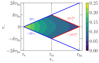
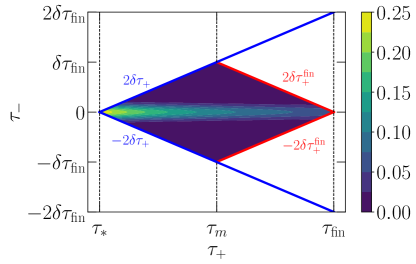
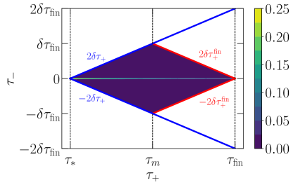
Figure 7: Integrand leading to the value of $\Delta_{0}$ assuming Kraichnan decorrelation for $p^{2}v_{\rm sw}^{2}=1$ (upper panel), $10$ (middle), and $100$ (lower), in the $k\to 0$ limit.

We observe that for large $p^{2}v_{\rm sw}^{2}\sim{\cal O}(10^{2})$, it is a good approximation to extend the integration limits to $\tau_{-}\in(-\infty,\infty)$, while the same is not true at smaller $p^{2}v_{\rm sw}^{2}\sim{\cal O}(1)$. In this case we find two limiting cases:

• if $\delta\tau_{\rm fin}\ll 1/(pv_{\rm sw})$, we expand $e^{-p^{2}v_{\rm sw}^{2}\tau_{-}^{2}}\sim 1$, since $\tau_{-}\in[0,\delta\tau_{\rm fin}]$ (see footnote 11). Then Eq. (89) yields the duration dependence found for the UETC of the sound shell model in the $k\to 0$ limit: $\ln^{2}(\tau_{\rm fin}{\cal H}_{*})$;

• if $\delta\tau_{\rm fin}\gg 1/(pv_{\rm sw})$, the approximation leading to Eq. (84) is justified, and we find the suppression factor $\Upsilon$ in the $k\to 0$ limit. As discussed above, this regime can also appear in the sound shell model when $k\delta\tau_{\rm fin}\gg 1$.

Therefore, the resulting dependence of the GW amplitude with $\delta\tau_{\rm fin}$ will change for different $v_{\rm sw}$ and it might be a combination of the different modes since one needs to integrate Eq. (63) over $p$ for the general time-dependence. In addition, as mentioned above, $v_{\rm sw}$ is also a function of $\tau_{1}$ and $\tau_{2}$, to ensure the positivity of the UETC kernel Auclair et al. (2022).

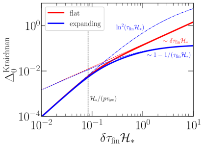
Figure 8: Dependence of the GW amplitude in the $k\to 0$ limit with the duration of the GW sourcing $\delta\tau_{\rm fin}$ for a Kraichnan decorrelation with $pv_{\rm sw}=12$ for a flat (red) and an expanding (blue) Universe. The two asymptotic limits are separated at $\delta\tau_{\rm fin}=1/(pv_{\rm sw})$, showing the $(\delta\tau_{\rm fin}{\cal H}_{*})^{2}$ scaling below this limit, and the suppression factor $\Upsilon$ above the limit.

We recover the previous result analytically when neglecting the expansion of the Universe,

$$\Delta_{0}^{\rm flat}(\delta\tau_{\rm fin},p)/{\cal H}_{*}^{2}= \,\frac{\sqrt{\pi}}{pv_{\rm sw}}\delta\tau_{\rm fin}\,{\rm Erf}\bigl{(}pv_{\rm sw}\delta\tau_{\rm fin}\bigr{)}$$

$$- \,\frac{1-e^{-p^{2}v_{\rm sw}^{2}\delta\tau_{\rm fin}^{2}}}{p^{2}v_{\rm sw}^{2}}\,,$$ (90)

where Erf$(x)$ is the error function. Taking the limits $\delta\tau_{\rm fin}\ll 1/(pv_{\rm sw})$ and $\delta\tau_{\rm fin}\gg 1/(pv_{\rm sw})$, we find the two asymptotic behaviors mentioned above,

$$\Delta_{0}^{\rm flat}(\delta\tau_{\rm fin}pv_{\rm sw}\ll 1) \,=(\delta\tau_{\rm fin}{\cal H}_{*})^{2},$$

$$\Delta_{0}^{\rm flat}(\delta\tau_{\rm fin}pv_{\rm sw}\gg 1) \,=\frac{\sqrt{\pi}\delta\tau_{\rm fin}{\cal H}_{*}}{pv_{\rm sw}/{\cal H}_{*}}.$$ (91)

Including the effect of the expansion of the Universe leads to the same short-duration regime, and the limit at large $\delta\tau_{\rm fin}pv_{\rm sw}$ becomes

$$\Delta(\delta\tau_{\rm fin}pv_{\rm sw}\gg 1)=\frac{\sqrt{\pi}}{pv_{\rm sw}/{\cal H}_{*}}\Upsilon(\delta\tau_{\rm fin}).$$ (92)

The two asymptotic limits are shown in Fig. (8), compared to Eq. (89) evaluated numerically. These results show how we can, in general, find both the quadratic and linear growth rates, depending on $v_{\rm sw}$, the specific value of $k$ (even in the $k\to 0$ limit), and the integrals over $p$ and $\tilde{p}$ performed to find the GW spectrum sourced by a stationary process.

VI GW spectrum from sound waves: results and template

In Secs. (IV) and (V) we have studied the GW spectrum in the low-frequency limit $k\to 0$, aiming to understand two characteristic features: the $k^{3}$ scaling, and the amplitude evolution with respect to the duration of the source. The present section is dedicated to the study of the shape of the GW spectrum at all frequencies.

For a direct comparison of our results for sound waves to those for other sources, e.g., decaying vortical turbulence, we adopt a similar normalization as in ref. Roper Pol et al. (2022b) (see also Sec. (III.3)).

VI.1 GW spectral shape

With Eq. (64) the GW spectrum can be expressed in terms of a normalized spectrum, $\zeta_{\rm GW}$,

$$\Omega_{\rm GW}(\delta\tau_{\rm fin}, \,R_{*},K)=3\,\bar{w}^{2}\,K^{3}\,\biggl{(}\frac{\Omega_{\rm K}}{{\cal K}}\biggr{)}^{2}{\cal C}$$

$$\times \,\,\tilde{\Delta}_{0}(\delta\tau_{\rm fin},R_{*})\,\zeta_{\rm GW}(\delta\tau_{\rm fin},K,R_{*})\,.$$ (93)

In order to describe the spectral modifications of $\zeta_{\rm GW}$ with respect to $\zeta_{\Pi}$, we introduce the function $\tilde{\Delta}\equiv\zeta_{\rm GW}/\zeta_{\Pi}$. Then Eq. (93) becomes

$$\Omega_{\rm GW}(\delta\tau_{\rm fin},R_{*}, \,K)=3\,\bar{w}^{2}\,K^{3}\,\biggl{(}\frac{\Omega_{\rm K}}{{\cal K}}\biggr{)}^{2}\,{\cal C}\,\zeta_{\Pi}(K)$$

$$\times \,\tilde{\Delta}_{0}(\delta\tau_{\rm fin},R_{*})\,\tilde{\Delta}(\delta\tau_{\rm fin},R_{*},K)\,.$$ (94)

$\tilde{\Delta}$ generalizes Eq. (63) to all values of $k$ and $\delta\tau_{\rm fin}$,

$$\tilde{\Delta}(\delta \tau_{\rm fin},R_{*},K)$$

$$= \,\frac{1}{{\cal C}\,\zeta_{\Pi}(K)\,\tilde{\Delta}_{0}(\delta\tau_{\rm fin},R_{*})}\int_{0}^{\infty}{\rm\,d}PP^{2}\zeta_{\rm kin}(P)$$

$$\times \,\int_{-1}^{1}(1-z^{2})^{2}\frac{\zeta_{\rm kin}(\tilde{P})}{\tilde{P}^{4}}\Delta(\delta\tau_{\rm fin},k,p,\tilde{p}){\rm\,d}z\,.$$ (95)

By construction we find that $\tilde{\Delta}\to 1$, when $\Delta$ does not depend on $p$ nor $k$, i.e., in the short-duration regime, or in the $k\to 0$ limit.

Hence, the parameters that determine the modifications of $\zeta_{\rm GW}$ with respect to $\zeta_{\Pi}$ are the source duration $\delta\tau_{\rm fin}$, and the characteristic scale $R_{*}=1/k_{*}$.

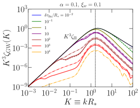
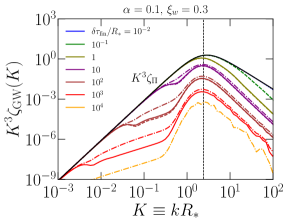
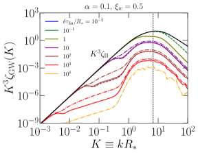
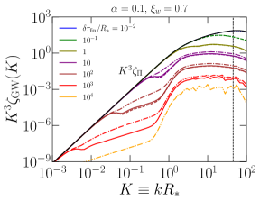
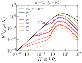
Figure 9: Normalized GW spectral shape $K^{3}\zeta_{\rm GW}$ (see Eq. (93)) for the benchmark phase transitions shown in Fig. (1) in the case of exponential nucleation. For comparison we show $K^{3}\zeta_{\Pi}$ (in black), expected in the range $k<1/\delta\tau_{\rm fin}$. The modifications with respect to $K^{3}\zeta_{\Pi}$ occur at $k>1/\delta\tau_{\rm fin}$, and different colors correspond to different values of $\delta\tau_{\rm fin}/R_{*}$. The exact modifications depend separately on both $R_{*}$ and $\delta\tau_{\rm fin}$, especially when $\delta\tau_{\rm fin}/R_{*}\gg 1$. Dotted, dashed, solid, and dash-dotted lines correspond to values $\delta\tau_{\rm fin}{\cal H}_{*}$ of $10^{-2}$, $10^{-1}$, 1, and $10$, respectively. The vertical lines indicate the estimated position of the GW peak, at $K\approx 0.8\,K_{\rm GW}$, where $K_{\rm GW}$ is the position where $K^{3}\zeta_{\Pi}$ is maximum (see values in Table 1). The second peak of $\zeta_{\Pi}$ appears also in $\zeta_{\rm GW}$, and is related to the inverse sound shell thickness $1/\Delta R_{*}\equiv\xi_{w}/(R_{*}|\xi_{w}-c_{s}|)$ Hindmarsh (2018). Hence, when $\xi_{w}$ is closer to $c_{\rm s}$, the second peak appears far from $1/R_{*}$, yielding a broad plateau around the peak. When $\xi_{w}$ diverges from $c_{\rm s}$, the second peak becomes closer to the first one at $K\sim 1$, and the plateau disappears.

Depending on how $k$ compares with the inverse source duration $1/\delta\tau_{\rm fin}$, the GW spectrum presents different behaviors.

In the regime where $k\lesssim 1/\delta\tau_{\rm fin}$, studied in Sec. (IV), $\tilde{\Delta}\to 1$. The dependence of the GW spectrum on the source duration $\delta\tau_{\rm fin}$ is then fully encoded in $\tilde{\Delta}_{0}=A\ln^{2}(\tau_{\rm fin}{\cal H}_{*})$, with $A\in[0.5,1]$, see Eq. (68). The amplitude in this regime does not depend on $R_{*}$, whose dependence only appears through the self-similar $K\equiv kR_{*}$. At the same time, the dependence on $K$ survives in $K^{3}\zeta_{\Pi}$, which, as shown in Fig. (2), follows a broken-power law that can be fit using Eq. (50). The amplitude of the GW spectrum depends on the specific spectral shape of the kinetic spectrum via the constants ${\cal K}$ and ${\cal C}$ (see Eqs. (43) and (46)). Table 1 presents values for the benchmark phase transitions considered here.

At wave numbers $k>1/\delta\tau_{\rm fin}$, the approximation leading to $\tilde{\Delta}\sim 1$ is no longer valid, and the function $\tilde{\Delta}(K)$ depends on both, $\delta\tau_{\rm fin}$ and $R_{*}$. As a consequence, in this range, the GW spectrum shows a complex dependence on $K$ and $\delta\tau_{\rm fin}$ that deviates with respect to the simple $K^{3}\zeta_{\Pi}$ causal growth. We expect the GW spectrum to transition from the causal branch at $k\delta\tau_{\rm fin}\ll 1$, toward the spectrum found in refs. Hindmarsh and Hijazi (2019); Guo et al. (2021) (see App. (B)), which is valid for $k\delta\tau_{\rm fin}\gg 1$, as discussed in Secs. (IV) and (V). This transition among the two asymptotic limits is, a priori, unknown and requires a numerical evaluation of Eq. (95).

Numerical examples of the resulting normalized GW spectra, $K^{3}\zeta_{\rm GW}$, are shown in Fig. (9) for the benchmark phase transitions of Fig. (1), and at different values of $\delta\tau_{\rm fin}$ and $R_{*}$. We find the predicted $K^{3}\zeta_{\Pi}$ scaling when $k<1/\delta\tau_{\rm fin}$, with the amplitude exactly given by Eq. (94) when setting $\tilde{\Delta}=1$.

A more complex structure appears at $k>1/\delta\tau_{\rm fin}$, where $\tilde{\Delta}\equiv\zeta_{\rm GW}/\zeta_{\Pi}$ plays a major role. To underline some generic features, we show $\tilde{\Delta}$ in Figure (10) at different $\delta\tau_{\rm fin}$ and $R_{*}$.

In the range $1/\delta\tau_{\rm fin}\lesssim k<1/R_{*}$, we find $\tilde{\Delta}\sim K^{-2}$, leading to the development of a linear GW spectrum in $k$. A similar transition from a $K^{3}$ to $K$ slope in the GW spectrum is also found for vortical (M)HD turbulence Roper Pol et al. (2020b, 2022a); Brandenburg et al. (2021b, a); Kahniashvili et al. (2021); Roper Pol et al. (2022b); Auclair et al. (2022), and is analytically described by the constant-in-time approximation Roper Pol et al. (2022b).

At larger $k$, a steep growth, $\Omega_{\rm GW}\sim K^{7}$, appears just below the peak of the spectrum. This result is close to the $K^{9}$ growth found in ref. Hindmarsh and Hijazi (2019). In fact, in this range, $1/\delta\tau_{\rm fin}\ll k\lesssim 1/R_{*}$, motivating the assumption $k\delta\tau_{\rm fin}\to\infty$, required to obtain the $K^{9}$ spectrum; see discussion in Sec. (V). Note however that, when the source duration becomes a non-negligible fraction of a Hubble time, $\delta\tau_{\rm fin}{\cal H}_{*}\gtrsim{\cal O}(10^{-1})$, the expansion of the Universe starts playing a significant role. In particular, it modifies not only the dependence of the GW spectrum on $\delta\tau_{\rm fin}$ but also its spectral shape through $\Delta$ in Eq. (95).

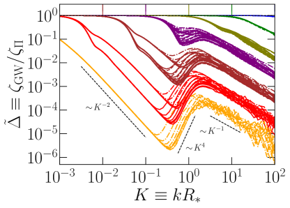
Figure 10: Ratio $\tilde{\Delta}\equiv\zeta_{\rm GW}/\zeta_{\Pi}$ for the benchmark phase transitions and parameters of Fig. (9). Line colors and styles are the same as those in Fig. (9).

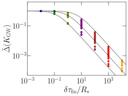
Figure 11: Dependence of the GW peak amplitude with $\delta\tau_{\rm fin}/R_{*}$, normalized to the value in the $\delta\tau_{\rm fin}\to 0$ limit. Each dot corresponds to a specific line in Fig. (10). The amplitude shows a universal trend with the product $\delta\tau_{\rm fin}/R_{*}$ that can be approximately fit empirically by the function $\bigl{(}1+\delta\tau_{\rm fin}/R_{*}\bigr{)}^{-1}$, intermediate black dashed line.

The peak amplitude of the GW spectrum, which we have previously estimated to be located at $K_{\rm GW}$, where $K^{3}\zeta_{\Pi}$ is maximum, is modified by $\tilde{\Delta}$ when the $k\lesssim 1/\delta\tau_{\rm fin}$ limit does not hold. We find that $\tilde{\Delta}$ modifies the position of the GW peak roughly to $K\approx 0.8\,K_{\rm GW}$ (see Fig. (9) and values in Table 1). In addition, $\tilde{\Delta}$ adds a dependence of the GW amplitude on $\delta\tau_{\rm fin}/R_{*}$, shown in Fig. (11). This modification at the peak is well approximated by the function $(1+\delta\tau_{\rm fin}/R_{*})^{-1}$. For the benchmark phase transitions, and the values of $\delta\tau_{\rm fin}$ and $R_{*}$ shown in Fig. (10), we estimate the accuracy of the fit within a factor of 5.

Around the peak, $\tilde{\Delta}_{0}\,\tilde{\Delta}$ depends linearly on the suppression factor, $\Upsilon$, and $R_{*}{\cal H}_{*}$. This result agrees with the one derived in App. (B), following the approximation of refs. Hindmarsh and Hijazi (2019); Guo et al. (2021), when $\delta\tau_{\rm fin}/R_{*}\gg 1$, such that the peak $1/R_{*}$ is within the $k\delta\tau_{\rm fin}\gg 1$ regime. For an accurate prediction of the amplitude at the peak, we thus take this value into account and multiply it by the value where the function $K^{3}\zeta_{\Pi}$ is maximal (see Table 1).

Finally, at large $K>1$, we find that the GW spectrum decreases as $1/K$ when compared to $K^{3}\zeta_{\Pi}$. Since the latter scales as $K^{-2}$ (see Fig. (2)), the GW spectrum decays as $K^{-3}$ at large values of $k$, which agrees with refs. Hindmarsh and Hijazi (2019); Jinno et al. (2021, 2023).

To compare the resulting spectral shape of GWs to that of ref. Hindmarsh and Hijazi (2019), where the function $\Delta$ is approximated by a Dirac delta function, we show in Fig. (12) the resulting GW spectra, obtained for a specific benchmark phase transition with $\alpha=0.1$ and $\xi_{w}=0.3$, for a range of $R_{*}$ and $\delta\tau_{\rm fin}$. The calculation of the GW spectra under the assumption of refs. Hindmarsh and Hijazi (2019); Guo et al. (2021) is given in App. (B).

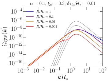
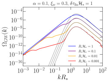
Figure 12: GW spectrum as a function of $kR_{*}$ for a benchmark phase transition with $\alpha=0.1$ and $\xi_{w}=0.3$, assuming exponential nucleation. The results are shown for different values of $R_{*}{\cal H}_{*}$, and $\delta\tau_{\rm fin}{\cal H}_{*}=0.01$ (upper panel) and $1$ (lower panel). For comparison, the grey lines correspond to the GW spectrum using the approximation of refs. Hindmarsh and Hijazi (2019); Guo et al. (2021) (see Eq. (103)).

We show that the GW spectrum found in ref. Hindmarsh and Hijazi (2019) is a correct description for the bump around and above the peak when $\delta\tau_{\rm fin}/R_{*}$ is sufficiently large (as described above), after taking into account the correction due to the expansion of the Universe Guo et al. (2021). The transition toward the GW spectrum in the “infinite duration” limit (given in App. (B)) is related to the one from the quadratic to linear growth that we have found in Sec. (V.2), since the approximation used to extend the limits of integration over $\tau_{-}$ to $\pm\infty$ in Eq. (80) is based on the assumption that $k\delta\tau_{\rm fin}\to\infty$. However, additional linear and cubic regimes appear in $\Omega_{\rm GW}$ at frequencies below the peak that were not found in refs. Hindmarsh and Hijazi (2019); Guo et al. (2021) since the $k\delta\tau_{\rm fin}\gg 1$ assumption does not hold in this range of frequencies. Moreover, when $\delta\tau_{\rm fin}/R_{*}<1$, the peak is in the regime $k_{*}<1/\delta\tau_{\rm fin}$, so that significant modifications of the GW spectrum may appear around the peak.

VI.2 Estimation of the source duration

Let us now discuss why the variables $\delta\tau_{\rm fin}$ and $R_{*}$ are not completely independent. The characteristic scale $R_{*}$ is determined by the mean bubble separation, which depends on the characteristics of the phase transition via $\beta$ and $\xi_{w}$ (see relation below Eq. (33)).

The evaluation of $\delta\tau_{\rm fin}$ requires further numerical studies to simulate the decay of the sound waves, as well as the development of turbulence.

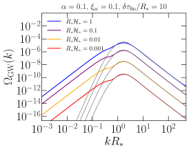
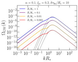
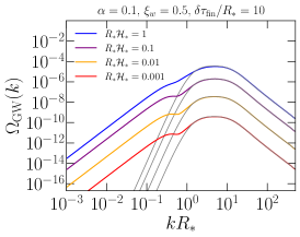
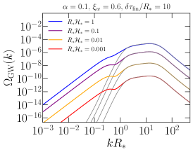
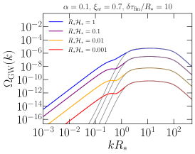
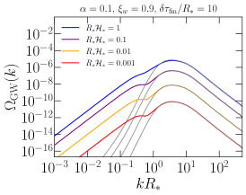
Figure 13: GW spectrum as a function of $kR_{*}$ for the benchmark phase transitions shown in Fig. (1). The results are shown for different values of $R_{*}{\cal H}_{*}=\{0.001,0.01,0.1,1\}$ and taking $\delta\tau_{\rm fin}=10R_{*}$, corresponding to the time expected to develop non-linearities for $\Omega_{\rm K}\sim 10^{-2}$. For comparison, the grey lines correspond to the GW spectrum using the approximation of refs. Hindmarsh and Hijazi (2019); Guo et al. (2021) (see Eq. (103)).

A first estimation of $\delta\tau_{\rm fin}$ is the eddy turnover time, i.e., the time that it takes the plasma to develop non-linearities, $\delta\tau_{\rm nl}\sim R_{*}/\sqrt{\Omega_{\rm K}}$ Caprini et al. (2020), and it directly depends on $R_{*}$. Setting $\delta\tau_{\rm fin}\sim\delta\tau_{\rm nl}$ and $\Omega_{\rm K}\sim 10^{-2}$ for the benchmark phase transitions with $\alpha=0.1$ (see Table 1), we find $\delta\tau_{\rm fin}/R_{*}\sim 10$. For this estimate, the condition $\delta\tau_{\rm fin}/R_{*}\gg 1$ is valid, and the prescription of refs. Hindmarsh and Hijazi (2019); Guo et al. (2021) gives a correct estimate of the amplitude around the peak. However, it fails at frequencies below the peak, as expected.

We show in Fig. (13) the GW spectrum found in the current work and compare it to the one given by Eq. (103), based on the assumptions of refs. Hindmarsh and Hijazi (2019); Guo et al. (2021), when we set $\delta\tau_{\rm fin}\sim 10R_{*}$. We find that, in this case, the suppression factor $\Upsilon$ is justified to describe the growth rate with $\tau_{\rm fin}$ at the peak. At frequencies below the peak, we find, in this case, that the linear growth with $k$ is almost completely absent and the causality tail, proportional to $k^{3}$, appears close to the peak, similar to the results of numerical simulations Jinno et al. (2023) and other analytical estimates Cai et al. (2023). However, for the exact dependence with $\delta\tau_{\rm fin}$ of the full spectral shape, we need to use the prescription developed in the current work. In particular, we find that the causality tail grows proportional to $\ln^{2}(\tau_{\rm fin}{\cal H}_{*})$.

VI.3 Present-time spectral amplitude

The present-time GW energy density spectrum, $\Omega_{\rm GW}^{0}(f)$ is a result of the computed spectrum redshifted from its time of generation to the present day,

$$h^{2}\Omega_{\rm GW}^{0}(f)=\biggl{(} \frac{a_{*}}{a_{0}}\biggr{)}^{4}\biggl{(}h\frac{H_{*}}{H_{0}}\biggr{)}^{2}\Omega_{\rm GW}(f)$$

$$\simeq \,1.6\times 10^{-5}\,\biggl{(}\frac{100}{g_{*}}\biggr{)}^{1\over 3}\Omega_{\rm GW}(f)\,,$$ (96)

where $a_{*}$ and $g_{*}$ correspond to the scale factor and the relativistic degrees of freedom at the time of GW generation, e.g., at the electroweak phase transition. $h=H_{0}/(100\,{\rm km}/{\rm s}/{\rm Mpc})$ takes into account the uncertainties on the present-time Hubble rate. Frequencies can be obtained from $k$ using the dispersion relation of GWs, $2\pi f=k$, and redshifting the mean-size of the bubbles $R_{*}$ to the present day,

$$R_{*}^{-1}= \,\frac{H_{*}}{R_{*}{\cal H}_{*}}\frac{a_{*}}{a_{0}}$$

$$\simeq \,\frac{1.65\times 10^{-5}\,{\rm\,Hz}}{R_{*}{\cal H}_{*}}\,\frac{T_{*}}{100{\rm\,GeV}}\biggl{(}\frac{g_{*}}{100}\biggr{)}^{1\over 6}\ .$$ (97)

VII Conclusions

We have studied the GW production from sound waves in a first-order phase transition during radiation domination. Sound waves are expected to be the dominant contribution to the SGWB, unless the bubbles run away, the phase transition is supercooled, or the efficiency in generating turbulence from bubble collisions is large.

We adopt the framework of the sound shell model to estimate the UETC of the velocity field Hindmarsh (2018). For the single-bubble velocity and energy density profiles, we follow the description of ref. Espinosa et al. (2010) and present the details of our calculation in an accompanying paper Roper Pol et al. (2023b). The sound-shell model predicted a $k^{9}$ growth of the spectrum at small frequencies $k$, and a linear dependence on the source duration $\delta\tau_{\rm fin}$ in ref. Hindmarsh and Hijazi (2019) that can be generalized to the suppression factor $\Upsilon=1-1/(1+\delta\tau_{\rm fin}{\cal H}_{*})$ when including the effect of the expansion of the Universe Guo et al. (2021). With this work, we have found that their prescription holds only in the regime $k\gg 1/\delta\tau_{\rm fin}$. We have addressed this issue and generalized their results to all frequencies.

Our results show that at small frequencies $k\to 0$, the GW spectrum presents a causal tail, proportional to $k^{3}$. The amplitude of this tail has a universal dependence on the physical parameters that describe the source. In particular, it is independent of $R_{*}$, and it grows with the duration of the source as $\ln^{2}(1+\delta\tau_{\rm fin}{\cal H}_{*})$, which yields a quadratic dependence when the source duration is short.

Around $k\gtrsim 1/\delta\tau_{\rm fin}$, an intermediate linear spectrum, $\Omega_{\rm GW}\sim k$, may appear, extending until a steep slope just below the peak takes over, which leads to the formation of a bump around the peak. When we estimate the duration of the GW sourcing as the time scale for the production of non-linearities in the plasma, we find that, for the benchmark phase transitions considered in this work with $\alpha=0.1$, $\delta\tau_{\rm fin}/R_{*}\sim 10$. In this case, the linear regime in $\Omega_{\rm GW}$ is almost absent, and the GW spectrum soon develops the causal $k^{3}$ tail at frequencies below the peak. When $\delta\tau_{\rm fin}/R_{*}$ becomes larger, the intermediate linear regime extends between the peak and the causal tail. This bump is a characteristic sign of a GW spectrum sourced by sound waves, since this distinctive feature does not appear in the GW spectrum sourced by vortical turbulence Roper Pol et al. (2020b); Brandenburg et al. (2021a); Kahniashvili et al. (2021); Brandenburg et al. (2021b); Roper Pol et al. (2022a, b); Auclair et al. (2022). A similar bump was previously found numerically for acoustic turbulence in ref. Roper Pol et al. (2020b) and confirmed in ref. Sharma et al. (2023). As long as the source duration is sufficiently large, $\delta\tau_{\rm fin}/R_{*}\gg 1$, we find that the amplitude around the peak is well described by the approach of refs. Hindmarsh and Hijazi (2019); Guo et al. (2021).

Our results reconcile the predictions of the sound shell model with the numerical simulations of ref. Jinno et al. (2023), where a cubic dependence of the GW spectrum at low $k$ is also found. Furthermore, they are in agreement with the findings of ref. Sharma et al. (2023), where numerical simulations are also performed, supporting the theoretical results of the sound shell model.

We have presented a theoretical description of the origin of the linear and quadratic growth with $\delta\tau_{\rm fin}$ that can appear when GWs are sourced by a general stationary process as, in the sound shell model, by a stationary UETC of the velocity field given by Eq. (39).

The resulting GW spectrum has been presented in a semi-analytical framework by separating each of the different contributions that can affect its final spectral shape and amplitude. Understanding each of the different contributions separately is important to test the validity of each of the underlying assumptions in future work. This framework allows for direct extensions of our results to include different models or assumptions.

We present the detailed calculation of the anisotropic stresses of the velocity field, following the sound shell model, in an accompanying paper Roper Pol et al. (2023b). We have also addressed the issue of causality that motivated the choice of initial conditions for sound waves in ref. Hindmarsh and Hijazi (2019), but we defer a detailed discussion of this issue to ref. Roper Pol et al. (2023b).

Our work has consequences on the interpretation of current observations of pulsar timing arrays under the assumption that the QCD phase transition is of first order. There are several analyses in the literature that have used the $k^{9}$ spectrum and the inclusion of a $k^{3}$ tail could lead to significantly different constraints on the phase transition parameters. This is especially important if one considers the smallest frequency bins reported by the PTA collaborations, which are below the characteristic frequency of the QCD phase transition where the signal is expected to be dominated by the $k^{3}$ tail or by the intermediate linear growth, $k$. Even at frequencies right below the peak, we expect the $k^{9}$ behavior to be shallower. Especially with the improvement of the PTA data in this range of frequencies expected in the next years, the study of the GW spectrum from sound waves with the presented modifications will become completely relevant.

Similarly, our model has implications for current estimations of the phase transition parameters that can be probed by LISA when one considers a first-order electroweak phase transition, since several analyses are currently using the $k^{9}$ model for the GW signal.

At larger frequencies, our model can be used to test the potential observability of higher-energy phase transitions with next-generation ground-based detectors, like Einstein Telescope or Cosmic Explorer, and to put constraints on the current and forthcoming observing runs by the LIGO–Virgo–KAGRA collaborations, especially in view of the advent of improvements in their sensitivities.

Appendix A Full time evolution of the GW spectrum

In this section, we compute the time evolution of the GW spectrum while the source is active, according to the sound shell model. The GW spectrum is usually averaged over oscillations with time, as we are interested in its present time observable, i.e., at very late times $\tau_{0}\gg\tau_{\rm fin}$. However, if the GW spectrum is compared with the results from simulations to, for example, test the validity of the sound shell model, it is required to compute its exact time evolution while the source is active at $\tau<\tau_{\rm fin}$. The average over oscillations is then not well motivated and it could lead to wrong results. We note that one has to pay particular attention to this aspect when using Weinberg’s formula as, for example, in refs. Jinno et al. (2021, 2023), since this approach already assumes that the GWs have reached their free propagation regime at all $k$, which can potentially lead to wrong results in the IR tail of the GW spectrum, and it does not allow to study their evolution with time.

We start with the GW spectrum, given by Eq. (12), and use the UETC of the anisotropic stresses of Eq. (23) with the stationary assumption for the velocity field UETC, see Eq. (39). We then find an expression analogous to that of Eq. (51) but in this case, the function $\Delta$ is a time-dependent expression given as

$$\Delta(\tau, \,k,p,\tilde{p})\equiv 2\int_{\tau_{*}}^{\tau}\frac{{\rm\,d}\tau_{1}}{\tau_{1}}\int_{\tau_{*}}^{\tau}\frac{{\rm\,d}\tau_{2}}{\tau_{2}}\cos(c_{\rm s}p\tau_{-})$$

$$\times \,\cos(c_{\rm s}\tilde{p}\tau_{-})\cos k(\tau-\tau_{1})\cos k(\tau-\tau_{2}).$$ (98)

We can express the product of $\cos$ as

$$\cos(c_{\rm s}p\tau_{-})\cos(c_{\rm s}\tilde{p}\tau_{-})=\frac{1}{2}\sum_{m=\pm 1}\cos(\hat{p}_{m}\tau_{-}),$$ (99)

with $\hat{p}_{m}=c_{\rm s}(p+m\tilde{p})$. Then, using $\cos k(\tau-\tau_{i})=\cos k\tau\cos k\tau_{i}+\sin k\tau\sin k\tau_{i}$ for $i=1,2$, one gets,

$$\Delta(\tau,k,p,\tilde{p})=\sum_{m=\pm 1}\Biggl{[}\biggl{(}\int_{\tau_{*}}^{\tau}\frac{{\rm\,d}\tau_{1}}{\tau_{1}}\bigl{[}\cos k\tau\cos k\tau_{1}+ \,\sin k\tau\sin k\tau_{1}]\cos(\hat{p}_{m}\tau_{1})\biggr{)}^{2}$$

$$+\biggl{(}\int_{\tau_{*}}^{\tau}\frac{{\rm\,d}\tau_{1}}{\tau_{1}}\bigl{[} \,\cos k\tau\cos k\tau_{1}+\sin k\tau\sin k\tau_{1}]\sin(\hat{p}_{m}\tau_{1})\biggr{)}^{2}\Biggr{]}$$

$$=\frac{1}{4}\sum_{m,n=\pm 1}\biggl{[}\Delta{\rm Ci}^{2}(\tau,\hat{p}_{mn})+\Delta{\rm Si}^{2}( \,\tau,\hat{p}_{mn})$$

$$+\cos 2k\tau\Bigl{(}\Delta{\rm Ci}(\tau,\hat{p}_{mn}) \Delta{\rm Ci}(\tau,\hat{p}_{m,-n})+\Delta{\rm Si}(\tau,\hat{p}_{mn})\Delta{\rm Si}(\tau,\hat{p}_{m,-n})\Bigr{)}\biggr{]}\,,$$ (100)

where the functions $\Delta{\rm Ci}_{mn}$ and $\Delta{\rm Si}_{mn}$ have been defined in Eqs. (57) and (58). We note that if one uses Eq. (56) substituting $\tau_{\rm fin}\to\tau$, Eq. (100) is not recovered, since the latter presents an additional term that is relevant during the phase of GW production. Hence, when comparing to numerical simulations, one should use Eq. (100) to study the validity of the stationary assumption for the UETC found in the sound shell model.

Appendix B GW spectrum in the infinite duration approximation

In this section, we take the approximation of $\Delta$ as a Dirac delta function (see Eq. (86)) that has been used in refs. Hindmarsh and Hijazi (2019); Guo et al. (2021) to find the GW spectrum from sound waves in the sound shell model approximation. We have shown in Secs. (IV) and (V) that this assumption is not valid in the $k\to 0$ limit and have presented the resulting GW spectrum in Sec. (VI), so we compare here what are the differences in the resulting spectral shape.

The GW spectrum, which we denote as HH19 (for Hindmarsh & Hijazi, 2019), is found substituting Eq. (86) into Eq. (51),

$$\Omega_{\rm GW}^{\rm HH19}(K)= \,\frac{3\pi}{2}K^{2}\,\Upsilon(\tau_{\rm fin})\,\frac{{\cal H}_{*}R_{*}}{c_{\rm s}}\,\bar{w}^{2}\,\biggl{(}\frac{\Omega_{\rm K}}{{\cal K}}\biggr{)}^{2}$$

$$\times\int_{0}^{\infty}P \,\zeta_{\rm kin}(P){\rm\,d}P\int_{|P-K|}^{P+K}(1-z^{2})^{2}\frac{{\rm\,d}\tilde{P}}{\tilde{P}^{3}}$$

$$\times\,\zeta_{\rm kin}(\tilde{P} \,)\,\delta(P+\tilde{P}-K/c_{\rm s})\ .$$ (101)

Under this assumption, one can perform the integral in Eq. (101) over $\tilde{P}$ by substituting $\tilde{P}=K/c_{\rm s}-P$ when $|K-P|\leq K/c_{\rm s}-P\leq K+P$, which yields the condition $P\in[P_{-},P_{+}]$ being $P_{\pm}={\textstyle{1\over 2}}K(1\pm c_{\rm s})/c_{\rm s}$, and

$$z=\frac{1}{c_{\rm s}}-\frac{K(1-c_{\rm s}^{2})}{2Pc_{\rm s}^{2}}.$$ (102)

Then the GW spectrum becomes

$$\Omega_{\rm GW}^{\rm HH19}(K)= \,\frac{3\pi}{2}K^{2}\,\Upsilon(\tau_{\rm fin})\,\frac{{\cal H}_{*}R_{*}}{c_{\rm s}}\,\bar{w}^{2}\,\biggl{(}\frac{\Omega_{\rm K}}{{\cal K}}\biggr{)}^{2}$$

$$\times \,\int_{P_{-}}^{P_{+}}P\zeta_{\rm kin}(P)(1-z^{2})^{2}$$

$$\,\times\frac{\zeta_{\rm kin}(K/c_{\rm s}-P)}{(K/c_{\rm s}-P)^{3}}{\rm\,d}P.$$ (103)

The resulting GW spectrum is shown in Figs. (12) and (13), compared with the full calculation. We find that Eq. (103) provides a good approximation when $k\gg 1/\delta\tau_{\rm fin}$.

References

- Kirzhnits and Linde (1976) D. A. Kirzhnits and Andrei D. Linde, “Symmetry Behavior in Gauge Theories,” Annals Phys. 101, 195–238 (1976).
- Coleman (1977) Sidney R. Coleman, “The Fate of the False Vacuum. 1. Semiclassical Theory,” Phys. Rev. D 15, 2929–2936 (1977), [Erratum: Phys.Rev.D 16, 1248 (1977)].
- Linde (1983) Andrei D. Linde, “Decay of the False Vacuum at Finite Temperature,” Nucl. Phys. B 216, 421 (1983), [Erratum: Nucl.Phys.B 223, 544 (1983)].
- Kajantie et al. (1997) K. Kajantie, M. Laine, K. Rummukainen, and Mikhail E. Shaposhnikov, “A Nonperturbative analysis of the finite T phase transition in SU(2) x U(1) electroweak theory,” Nucl. Phys. B 493, 413–438 (1997), arXiv:hep-lat/9612006 .
- Stephanov (2006) M. A. Stephanov, “QCD critical point and complex chemical potential singularities,” Phys. Rev. D 73, 094508 (2006), arXiv:hep-lat/0603014 .
- Caprini et al. (2020) Chiara Caprini et al., “Detecting gravitational waves from cosmological phase transitions with LISA: an update,” JCAP 03, 024 (2020), arXiv:1910.13125 [astro-ph.CO] .
- Schwarz and Stuke (2009) Dominik J. Schwarz and Maik Stuke, “Lepton asymmetry and the cosmic QCD transition,” JCAP 11, 025 (2009), [Erratum: JCAP 10, E01 (2010)], arXiv:0906.3434 [hep-ph] .
- Wygas et al. (2018) Mandy M. Wygas, Isabel M. Oldengott, Dietrich Bödeker, and Dominik J. Schwarz, “Cosmic QCD Epoch at Nonvanishing Lepton Asymmetry,” Phys. Rev. Lett. 121, 201302 (2018), arXiv:1807.10815 [hep-ph] .
- Middeldorf-Wygas et al. (2022) Mandy M. Middeldorf-Wygas, Isabel M. Oldengott, Dietrich Bödeker, and Dominik J. Schwarz, “Cosmic QCD transition for large lepton flavor asymmetries,” Phys. Rev. D 105, 123533 (2022), arXiv:2009.00036 [hep-ph] .
- Vovchenko et al. (2021) Volodymyr Vovchenko, Bastian B. Brandt, Francesca Cuteri, Gergely Endrődi, Fazlollah Hajkarim, and Jürgen Schaffner-Bielich, “Pion Condensation in the Early Universe at Nonvanishing Lepton Flavor Asymmetry and Its Gravitational Wave Signatures,” Phys. Rev. Lett. 126, 012701 (2021), arXiv:2009.02309 [hep-ph] .
- Cao (2023) Gaoqing Cao, “First-order QCD transition in a primordial magnetic field,” Phys. Rev. D 107, 014021 (2023), arXiv:2210.09794 [nucl-th] .
- Steinhardt (1982) Paul Joseph Steinhardt, “Relativistic Detonation Waves and Bubble Growth in False Vacuum Decay,” Phys. Rev. D 25, 2074 (1982).
- Enqvist et al. (1992) K. Enqvist, J. Ignatius, K. Kajantie, and K. Rummukainen, “Nucleation and bubble growth in a first order cosmological electroweak phase transition,” Phys. Rev. D 45, 3415–3428 (1992).
- Ignatius et al. (1994) J. Ignatius, K. Kajantie, H. Kurki-Suonio, and M. Laine, “The growth of bubbles in cosmological phase transitions,” Phys. Rev. D 49, 3854–3868 (1994), arXiv:astro-ph/9309059 .
- Witten (1984) Edward Witten, “Cosmic Separation of Phases,” Phys. Rev. D 30, 272–285 (1984).
- Hogan (1986) C. J. Hogan, “Gravitational radiation from cosmological phase transitions,” Mon. Not. Roy. Astron. Soc. 218, 629–636 (1986).
- Kosowsky et al. (1992a) Arthur Kosowsky, Michael S. Turner, and Richard Watkins, “Gravitational radiation from colliding vacuum bubbles,” Phys. Rev. D 45, 4514–4535 (1992a).
- Kosowsky et al. (1992b) Arthur Kosowsky, Michael S. Turner, and Richard Watkins, “Gravitational waves from first order cosmological phase transitions,” Phys. Rev. Lett. 69, 2026–2029 (1992b).
- Kosowsky and Turner (1993) Arthur Kosowsky and Michael S. Turner, “Gravitational radiation from colliding vacuum bubbles: envelope approximation to many bubble collisions,” Phys. Rev. D 47, 4372–4391 (1993), arXiv:astro-ph/9211004 .
- Caprini et al. (2008) Chiara Caprini, Ruth Durrer, and Geraldine Servant, “Gravitational wave generation from bubble collisions in first-order phase transitions: An analytic approach,” Phys. Rev. D 77, 124015 (2008), arXiv:0711.2593 [astro-ph] .
- Huber and Konstandin (2008a) Stephan J. Huber and Thomas Konstandin, “Gravitational Wave Production by Collisions: More Bubbles,” JCAP 09, 022 (2008a), arXiv:0806.1828 [hep-ph] .
- Jinno and Takimoto (2019) Ryusuke Jinno and Masahiro Takimoto, “Gravitational waves from bubble dynamics: Beyond the Envelope,” JCAP 01, 060 (2019), arXiv:1707.03111 [hep-ph] .
- Cutting et al. (2018) Daniel Cutting, Mark Hindmarsh, and David J. Weir, “Gravitational waves from vacuum first-order phase transitions: from the envelope to the lattice,” Phys. Rev. D 97, 123513 (2018), arXiv:1802.05712 [astro-ph.CO] .
- Hindmarsh et al. (2014) Mark Hindmarsh, Stephan J. Huber, Kari Rummukainen, and David J. Weir, “Gravitational waves from the sound of a first order phase transition,” Phys. Rev. Lett. 112, 041301 (2014), arXiv:1304.2433 [hep-ph] .
- Hindmarsh et al. (2015) Mark Hindmarsh, Stephan J. Huber, Kari Rummukainen, and David J. Weir, “Numerical simulations of acoustically generated gravitational waves at a first order phase transition,” Phys. Rev. D 92, 123009 (2015), arXiv:1504.03291 [astro-ph.CO] .
- Hindmarsh (2018) Mark Hindmarsh, “Sound shell model for acoustic gravitational wave production at a first-order phase transition in the early Universe,” Phys. Rev. Lett. 120, 071301 (2018), arXiv:1608.04735 [astro-ph.CO] .
- Hindmarsh et al. (2017) Mark Hindmarsh, Stephan J. Huber, Kari Rummukainen, and David J. Weir, “Shape of the acoustic gravitational wave power spectrum from a first order phase transition,” Phys. Rev. D 96, 103520 (2017), [Erratum: Phys.Rev.D 101, 089902 (2020)], arXiv:1704.05871 [astro-ph.CO] .
- Hindmarsh and Hijazi (2019) Mark Hindmarsh and Mulham Hijazi, “Gravitational waves from first order cosmological phase transitions in the Sound Shell Model,” JCAP 12, 062 (2019), arXiv:1909.10040 [astro-ph.CO] .
- Jinno et al. (2021) Ryusuke Jinno, Thomas Konstandin, and Henrique Rubira, “A hybrid simulation of gravitational wave production in first-order phase transitions,” JCAP 04, 014 (2021), arXiv:2010.00971 [astro-ph.CO] .
- Jinno et al. (2023) Ryusuke Jinno, Thomas Konstandin, Henrique Rubira, and Isak Stomberg, “Higgsless simulations of cosmological phase transitions and gravitational waves,” JCAP 02, 011 (2023), arXiv:2209.04369 [astro-ph.CO] .
- Kosowsky et al. (2002) Arthur Kosowsky, Andrew Mack, and Tinatin Kahniashvili, “Gravitational radiation from cosmological turbulence,” Phys. Rev. D 66, 024030 (2002), arXiv:astro-ph/0111483 .
- Gogoberidze et al. (2007) Grigol Gogoberidze, Tina Kahniashvili, and Arthur Kosowsky, “The Spectrum of Gravitational Radiation from Primordial Turbulence,” Phys. Rev. D 76, 083002 (2007), arXiv:0705.1733 [astro-ph] .
- Caprini et al. (2009a) Chiara Caprini, Ruth Durrer, Thomas Konstandin, and Geraldine Servant, “General Properties of the Gravitational Wave Spectrum from Phase Transitions,” Phys. Rev. D 79, 083519 (2009a), arXiv:0901.1661 [astro-ph.CO] .
- Caprini et al. (2009b) Chiara Caprini, Ruth Durrer, and Geraldine Servant, “The stochastic gravitational wave background from turbulence and magnetic fields generated by a first-order phase transition,” JCAP 12, 024 (2009b), arXiv:0909.0622 [astro-ph.CO] .
- Niksa et al. (2018) Peter Niksa, Martin Schlederer, and Günter Sigl, “Gravitational Waves produced by Compressible MHD Turbulence from Cosmological Phase Transitions,” Class. Quant. Grav. 35, 144001 (2018), arXiv:1803.02271 [astro-ph.CO] .
- Roper Pol et al. (2020a) Alberto Roper Pol, Axel Brandenburg, Tina Kahniashvili, Arthur Kosowsky, and Sayan Mandal, “The timestep constraint in solving the gravitational wave equations sourced by hydromagnetic turbulence,” Geophys. Astrophys. Fluid Dynamics 114, 130–161 (2020a), arXiv:1807.05479 [physics.flu-dyn] .
- Roper Pol et al. (2020b) Alberto Roper Pol, Sayan Mandal, Axel Brandenburg, Tina Kahniashvili, and Arthur Kosowsky, “Numerical simulations of gravitational waves from early-universe turbulence,” Phys. Rev. D 102, 083512 (2020b), arXiv:1903.08585 [astro-ph.CO] .
- Kahniashvili et al. (2021) Tina Kahniashvili, Axel Brandenburg, Grigol Gogoberidze, Sayan Mandal, and Alberto Roper Pol, “Circular polarization of gravitational waves from early-Universe helical turbulence,” Phys. Rev. Res. 3, 013193 (2021), arXiv:2011.05556 [astro-ph.CO] .
- Brandenburg et al. (2021a) Axel Brandenburg, Emma Clarke, Yutong He, and Tina Kahniashvili, “Can we observe the QCD phase transition-generated gravitational waves through pulsar timing arrays?” (2021a), arXiv:2102.12428 [astro-ph.CO] .
- Brandenburg et al. (2021b) Axel Brandenburg, Grigol Gogoberidze, Tina Kahniashvili, Sayan Mandal, Alberto Roper Pol, and Nakul Shenoy, “The scalar, vector, and tensor modes in gravitational wave turbulence simulations,” Class. Quant. Grav. 38, 145002 (2021b), arXiv:2103.01140 [gr-qc] .
- Roper Pol et al. (2022a) Alberto Roper Pol, Sayan Mandal, Axel Brandenburg, and Tina Kahniashvili, “Polarization of gravitational waves from helical MHD turbulent sources,” JCAP 04, 019 (2022a), arXiv:2107.05356 [gr-qc] .
- Roper Pol et al. (2022b) Alberto Roper Pol, Chiara Caprini, Andrii Neronov, and Dmitri Semikoz, “Gravitational wave signal from primordial magnetic fields in the Pulsar Timing Array frequency band,” Phys. Rev. D 105, 123502 (2022b), arXiv:2201.05630 [astro-ph.CO] .
- Auclair et al. (2022) Pierre Auclair, Chiara Caprini, Daniel Cutting, Mark Hindmarsh, Kari Rummukainen, Danièle A. Steer, and David J. Weir, “Generation of gravitational waves from freely decaying turbulence,” JCAP 09, 029 (2022), arXiv:2205.02588 [astro-ph.CO] .
- Sharma and Brandenburg (2022) Ramkishor Sharma and Axel Brandenburg, “Low frequency tail of gravitational wave spectra from hydromagnetic turbulence,” Phys. Rev. D 106, 103536 (2022), arXiv:2206.00055 [astro-ph.CO] .
- Caprini and Figueroa (2018) Chiara Caprini and Daniel G. Figueroa, “Cosmological Backgrounds of Gravitational Waves,” Class. Quant. Grav. 35, 163001 (2018), arXiv:1801.04268 [astro-ph.CO] .
- Espinosa et al. (2010) Jose R. Espinosa, Thomas Konstandin, Jose M. No, and Geraldine Servant, “Energy Budget of Cosmological First-order Phase Transitions,” JCAP 06, 028 (2010), arXiv:1004.4187 [hep-ph] .
- Bodeker and Moore (2009) Dietrich Bodeker and Guy D. Moore, “Can electroweak bubble walls run away?” JCAP 05, 009 (2009), arXiv:0903.4099 [hep-ph] .
- Bodeker and Moore (2017) Dietrich Bodeker and Guy D. Moore, “Electroweak Bubble Wall Speed Limit,” JCAP 05, 025 (2017), arXiv:1703.08215 [hep-ph] .
- Caprini et al. (2016) Chiara Caprini et al., “Science with the space-based interferometer eLISA. II: Gravitational waves from cosmological phase transitions,” JCAP 04, 001 (2016), arXiv:1512.06239 [astro-ph.CO] .
- von Harling and Servant (2018) Benedict von Harling and Geraldine Servant, “QCD-induced Electroweak Phase Transition,” JHEP 01, 159 (2018), arXiv:1711.11554 [hep-ph] .
- Kobakhidze et al. (2017) Archil Kobakhidze, Cyril Lagger, Adrian Manning, and Jason Yue, “Gravitational waves from a supercooled electroweak phase transition and their detection with pulsar timing arrays,” Eur. Phys. J. C 77, 570 (2017), arXiv:1703.06552 [hep-ph] .
- Kosowsky (1996) Arthur Kosowsky, “Cosmic microwave background polarization,” Annals Phys. 246, 49–85 (1996), arXiv:astro-ph/9501045 .
- Quashnock et al. (1989) Jean M. Quashnock, Abraham Loeb, and David N. Spergel, “Magnetic Field Generation During the Cosmological QCD Phase Transition,” Astrophys. J. Lett. 344, L49–L51 (1989).
- Brandenburg et al. (1996) Axel Brandenburg, Kari Enqvist, and Poul Olesen, “Large scale magnetic fields from hydromagnetic turbulence in the very early universe,” Phys. Rev. D 54, 1291–1300 (1996), arXiv:astro-ph/9602031 .
- Ahonen and Enqvist (1996) Jarkko Ahonen and Kari Enqvist, “Electrical conductivity in the early universe,” Phys. Lett. B 382, 40–44 (1996), arXiv:hep-ph/9602357 .
- Arnold et al. (2000) Peter Brockway Arnold, Guy D. Moore, and Laurence G. Yaffe, “Transport coefficients in high temperature gauge theories. 1. Leading log results,” JHEP 11, 001 (2000), arXiv:hep-ph/0010177 .
- Cutting et al. (2020) Daniel Cutting, Mark Hindmarsh, and David J. Weir, “Vorticity, kinetic energy, and suppressed gravitational wave production in strong first order phase transitions,” Phys. Rev. Lett. 125, 021302 (2020), arXiv:1906.00480 [hep-ph] .
- Roper Pol et al. (2023a) A. Roper Pol, A. Neronov, C. Caprini, T. Boyer, and D. Semikoz, “LISA and -ray telescopes as multi-messenger probes of a first-order cosmological phase transition,” (2023a), arXiv:2307.10744 [astro-ph.CO] .
- Guo et al. (2021) Huai-Ke Guo, Kuver Sinha, Daniel Vagie, and Graham White, “Phase Transitions in an Expanding Universe: Stochastic Gravitational Waves in Standard and Non-Standard Histories,” JCAP 01, 001 (2021), arXiv:2007.08537 [hep-ph] .
- Cai et al. (2023) Rong-Gen Cai, Shao-Jiang Wang, and Zi-Yan Yuwen, “Hydrodynamic sound shell model,” (2023), arXiv:2305.00074 [gr-qc] .
- Antoniadis et al. (2023a) J. Antoniadis et al. (EPTA), “The second data release from the European Pulsar Timing Array III. Search for gravitational wave signals,” (2023a), arXiv:2306.16214 [astro-ph.HE] .
- Antoniadis et al. (2023b) J. Antoniadis et al. (EPTA), “The second data release from the European Pulsar Timing Array: V. Implications for massive black holes, dark matter and the early Universe,” (2023b), arXiv:2306.16227 [astro-ph.CO] .
- Agazie et al. (2023) Gabriella Agazie et al. (NANOGrav), “The NANOGrav 15 yr Data Set: Evidence for a Gravitational-wave Background,” Astrophys. J. Lett. 951, L8 (2023), arXiv:2306.16213 [astro-ph.HE] .
- Afzal et al. (2023) Adeela Afzal et al. (NANOGrav), “The NANOGrav 15 yr Data Set: Search for Signals from New Physics,” Astrophys. J. Lett. 951, L11 (2023), arXiv:2306.16219 [astro-ph.HE] .
- Reardon et al. (2023) Daniel J. Reardon et al., “Search for an Isotropic Gravitational-wave Background with the Parkes Pulsar Timing Array,” Astrophys. J. Lett. 951, L6 (2023), arXiv:2306.16215 [astro-ph.HE] .
- Xu et al. (2023) Heng Xu et al., “Searching for the Nano-Hertz Stochastic Gravitational Wave Background with the Chinese Pulsar Timing Array Data Release I,” Res. Astron. Astrophys. 23, 075024 (2023), arXiv:2306.16216 [astro-ph.HE] .
- Madge et al. (2023) Eric Madge, Enrico Morgante, Cristina Puchades-Ibáñez, Nicklas Ramberg, Wolfram Ratzinger, Sebastian Schenk, and Pedro Schwaller, “Primordial gravitational waves in the nano-Hertz regime and PTA data – towards solving the GW inverse problem,” (2023), arXiv:2306.14856 [hep-ph] .
- Bringmann et al. (2023) Torsten Bringmann, Paul Frederik Depta, Thomas Konstandin, Kai Schmidt-Hoberg, and Carlo Tasillo, “Does NANOGrav observe a dark sector phase transition?” (2023), arXiv:2306.09411 [astro-ph.CO] .
- Zu et al. (2023) Lei Zu, Chi Zhang, Yao-Yu Li, Yu-Chao Gu, Yue-Lin Sming Tsai, and Yi-Zhong Fan, “Mirror QCD phase transition as the origin of the nanohertz Stochastic Gravitational-Wave Background,” (2023), arXiv:2306.16769 [astro-ph.HE] .
- Addazi et al. (2023) Andrea Addazi, Yi-Fu Cai, Antonino Marciano, and Luca Visinelli, “Have pulsar timing array methods detected a cosmological phase transition?” (2023), arXiv:2306.17205 [astro-ph.CO] .
- Han et al. (2023) Chengcheng Han, Ke-Pan Xie, Jin Min Yang, and Mengchao Zhang, “Self-interacting dark matter implied by nano-Hertz gravitational waves,” (2023), arXiv:2306.16966 [hep-ph] .
- Megias et al. (2023) Eugenio Megias, Germano Nardini, and Mariano Quiros, “Pulsar Timing Array Stochastic Background from light Kaluza-Klein resonances,” (2023), arXiv:2306.17071 [hep-ph] .
- Li and Xie (2023) Shao-Ping Li and Ke-Pan Xie, “Collider test of nano-Hertz gravitational waves from pulsar timing arrays,” Phys. Rev. D 108, 055018 (2023), arXiv:2307.01086 [hep-ph] .
- Di Bari and Rahat (2023) Pasquale Di Bari and Moinul Hossain Rahat, “The split majoron model confronts the NANOGrav signal,” (2023), arXiv:2307.03184 [hep-ph] .
- Bai et al. (2023) Yang Bai, Ting-Kuo Chen, and Mrunal Korwar, “QCD-Collapsed Domain Walls: QCD Phase Transition and Gravitational Wave Spectroscopy,” (2023), arXiv:2306.17160 [hep-ph] .
- Ghosh et al. (2023) Tathagata Ghosh, Anish Ghoshal, Huai-Ke Guo, Fazlollah Hajkarim, Stephen F. King, Kuver Sinha, Xin Wang, and Graham White, “Did we hear the sound of the Universe boiling? Analysis using the full fluid velocity profiles and NANOGrav 15-year data,” (2023), arXiv:2307.02259 [astro-ph.HE] .
- Figueroa et al. (2023) Daniel G. Figueroa, Mauro Pieroni, Angelo Ricciardone, and Peera Simakachorn, “Cosmological Background Interpretation of Pulsar Timing Array Data,” (2023), arXiv:2307.02399 [astro-ph.CO] .
- Amaro-Seoane et al. (2017) Pau Amaro-Seoane et al. (LISA), “Laser Interferometer Space Antenna,” (2017), arXiv:1702.00786 [astro-ph.IM] .
- Caprini et al. (2019) Chiara Caprini, Daniel G. Figueroa, Raphael Flauger, Germano Nardini, Marco Peloso, Mauro Pieroni, Angelo Ricciardone, and Gianmassimo Tasinato, “Reconstructing the spectral shape of a stochastic gravitational wave background with LISA,” JCAP 11, 017 (2019), arXiv:1906.09244 [astro-ph.CO] .
- Gowling and Hindmarsh (2021) Chloe Gowling and Mark Hindmarsh, “Observational prospects for phase transitions at LISA: Fisher matrix analysis,” (2021), arXiv:2106.05984 [astro-ph.CO] .
- Giese et al. (2021) Felix Giese, Thomas Konstandin, and Jorinde van de Vis, “Finding sound shells in LISA mock data using likelihood sampling,” JCAP 11, 002 (2021), arXiv:2107.06275 [astro-ph.CO] .
- Boileau et al. (2023) Guillaume Boileau, Nelson Christensen, Chloe Gowling, Mark Hindmarsh, and Renate Meyer, “Prospects for LISA to detect a gravitational-wave background from first order phase transitions,” JCAP 02, 056 (2023), arXiv:2209.13277 [gr-qc] .
- Gowling et al. (2023) Chloe Gowling, Mark Hindmarsh, Deanna C. Hooper, and Jesús Torrado, “Reconstructing physical parameters from template gravitational wave spectra at LISA: first order phase transitions,” JCAP 04, 061 (2023), arXiv:2209.13551 [astro-ph.CO] .
- Romero et al. (2021) Alba Romero, Katarina Martinovic, Thomas A. Callister, Huai-Ke Guo, Mario Martínez, Mairi Sakellariadou, Feng-Wei Yang, and Yue Zhao, “Implications for First-Order Cosmological Phase Transitions from the Third LIGO-Virgo Observing Run,” Phys. Rev. Lett. 126, 151301 (2021), arXiv:2102.01714 [hep-ph] .
- Roper Pol et al. (2023b) Alberto Roper Pol, Simona Procacci, Chiara Caprini, and Antonino Salvino Midiri, “Kinetic spectrum from the sound shell model,” in preparation (2023b).
- Isserlis (1916) L. Isserlis, “On certain probable errors and correlation of multiple frequency distributions with skew regression,” Biometrika 11, 185 (1916).
- Monin and Yaglom (1975) A. S. Monin and A. M. Yaglom, Statistical fluid mechanics: Mechanics of turbulence, Vol. 2 (MIT press, Cambridge, MA, U.S.A., 1975).
- Caprini et al. (2004) Chiara Caprini, Ruth Durrer, and Tina Kahniashvili, “The Cosmic microwave background and helical magnetic fields: The Tensor mode,” Phys. Rev. D 69, 063006 (2004), arXiv:astro-ph/0304556 .
- Sharma et al. (2023) Ramkishor Sharma, Jani Dahl, Axel Brandenburg, and Mark Hindmarsh, “Shallow relic gravitational wave spectrum with acoustic peak,” (2023), arXiv:2308.12916 [gr-qc] .
- Huber and Konstandin (2008b) Stephan J. Huber and Thomas Konstandin, “Production of gravitational waves in the nMSSM,” JCAP 05, 017 (2008b), arXiv:0709.2091 [hep-ph] .
- Weir (2018) David J. Weir, “Gravitational waves from a first order electroweak phase transition: a brief review,” Phil. Trans. Roy. Soc. Lond. A 376, 20170126 (2018), arXiv:1705.01783 [hep-ph] .
- Hindmarsh et al. (2021) Mark B. Hindmarsh, Marvin Lüben, Johannes Lumma, and Martin Pauly, “Phase transitions in the early universe,” SciPost Phys. Lect. Notes 24, 1 (2021), arXiv:2008.09136 [astro-ph.CO] .
- Kraichnan (1965) Robert H. Kraichnan, “Inertial-Range Spectrum of Hydromagnetic Turbulence,” Phys. Fluids 8, 1385–1387 (1965).
- Pen and Turok (2016) Ue-Li Pen and Neil Turok, “Shocks in the Early Universe,” Phys. Rev. Lett. 117, 131301 (2016), arXiv:1510.02985 [astro-ph.CO] .