Astronomical interferometry using continuous variable quantum teleportation

Abstract

We propose a method to build an astronomical interferometer using continuous variable quantum teleportation to overcome the transmission loss between distant telescopes. The scheme relies on two-mode squeezed states shared by distant telescopes as entanglement resources, which are distributed using continuous variable quantum repeaters. We find the optimal measurement on the teleported states, which uses beam-splitters and photon-number-resolved detection. Compared to prior proposals relying on discrete states, our scheme has the advantages of using linear optics to implement the scheme without wasting stellar photons and making use of multiphoton events, which are regarded as noise in previous discrete schemes.

1 introduction

Interferometric imaging is a widely used method in astronomy that employs multiple spatially separated telescopes for enhanced resolution and sensitivity. It is based on the Van Cittert-Zernike theorem [1], which shows one can determine the Fourier component of the intensity distribution in the source plane by interfering with the light received at different locations in the image plane and measuring the mutual coherence function. The successful application of interferometer arrays in astronomy, especially at radio frequencies, provides a very powerful tool for high-resolution imaging. For example, the first image of a supermassive black hole at the center of the Messier 87 Galaxy was provided by a radio interferometer array [2]. However, unlike radio wavelengths, for which the light is directly measured and recorded separately at each telescope [3], at optical wavelengths the light signals received at different locations in the interferometer array are at frequencies too high to be recorded, so instead they are brought together to interfere in what is referred to as the direct-detection method [4]. However, in this method there is unavoidable transmission loss while bringing light from distant telescopes together, and this limits the length of the baseline and hence the resolution of optical interferometer arrays. It is also possible to measure the coherence function through local measurements with a shared phase reference, but for weak thermal sources at optical wavelengths the mean photon number per temporal mode is much less than one, and it is not possible to distinguish the vacuum and single photon states locally. This strongly degrades the sensitivity of local measurements at each telescope [5].

Several proposals have been made recently that overcome transmission loss based on quantum networks [6, 7, 8]. Taking advantage of entanglement resources provided by the quantum network, the coherence function can be measured without directly interfering the light and with sensitivity comparable to the direct-detection method. These proposals can be understood qualitatively as leveraging teleportation from one telescope to another using entanglement resources shared by the distant telescopes. Transmission loss will affect the distribution of the entanglement resource, which can be overcome by quantum repeaters. A quantum repeater distills high-fidelity entangled states from many copies of distributed noisy entangled states between nearby quantum nodes and creates long-distance entanglement from short-distance entanglement using entanglement swapping [9]. Although this in principle means we can arbitrarily increase the baseline between telescopes, these proposals have their own difficulties in implementation. Reference [6] requires an excessive amount of distributed entangled photons. Reference [7, 8] exploits quantum memory to encode the arrival time of the stellar photons to avoid the wasting of entanglement resources when a vacuum state is received. This approach introduces the extra difficulties of implementing two-qubit quantum gates and requires reliable quantum memories.

In this paper, we extend the concept of quantum-network-based astronomical interferometry to another version of quantum teleportation, namely, continuous variable (CV) quantum teleportation [10, 11, 12]. Compared to Ref. [6, 7, 8], where the weak thermal light received from the astronomical source is approximated as discrete states, namely, vacuum or single photon states, here we directly work with the exact thermal state, which is a Gaussian state with representation in terms of Gaussian functions [13]. Our scheme relies on the analog of Einstein-Podolsky-Rosen (EPR) states in continuous variables, i.e. the two-mode squeezed states. Here we discuss the sensitivity of our scheme under transmission loss and construct optimal measurements for estimating the coherence function from the teleported state. We find that the required repetition rate to cover all temporal modes is approximately 150 GHz at wavelength $\lambda=800\;\text{nm}$, much higher than state-of-the-art pulsed squeezing with 86.5 MHz repetition rate and 5.88 dB squeezing level [14]. Nevertheless, our method still provides a meaningful alternative for building an astronomical interferometer that may be more feasible than other quantum network protocols, depending on the development of quantum repeaters. In particular, our scheme can exploit multiphoton events that are discarded as noise in Ref. [6, 7, 8], which can provide an advantage when imaging a stronger astronomical source or at a longer wavelength.

2 Teleportation of stellar light

In this section, we consider the CV teleportation of stellar light from one telescope to another telescope. As shown in Fig. 1, we assume the bipartite thermal state $\rho_{s}$ of mode $\hat{a}_{1,2}$ from the astronomical source is received by two telescopes $A,B$ in an interferometer array [15], with the form:

$$\rho_{s}=\int \frac{d^{2}\alpha d^{2}\beta}{\pi^{2}\det\Gamma}\ket{\alpha,\beta}\bra{\alpha,\beta}$$ (1)

$$\times\exp[-\begin{pmatrix}\alpha*\hfil&\beta^{*}\end{pmatrix}\Gamma^{-1}\begin{pmatrix}\alpha\\ \beta\end{pmatrix}]$$

$$\Gamma=\frac{\epsilon}{2}\begin{pmatrix}1&g\\ g^{*}&1\end{pmatrix},$$ (2)

where $g=|g|e^{i\theta}$ is the coherence function we want to measure and $\epsilon$ is the mean photon number per temporal mode. Any Gaussian state can be completely described with its mean value $x_{i}=\tr(\rho_{s}\hat{x}_{i})$ and covariance matrix $V_{ij}=\frac{1}{2}\tr[\rho_{s}(\Delta\hat{x}_{i}\Delta\hat{x}_{j}+\Delta\hat{x}_{j}\Delta\hat{x}_{i})]$, where $\hat{\vec{x}}=(\hat{q}_{1},\hat{p}_{1},\hat{q}_{2},\hat{p}_{2})^{T}$, $\hat{q}_{i}=(\hat{a}_{i}+\hat{a}_{i}^{\dagger})/\sqrt{2}$, $\hat{p}_{i}=(\hat{a}_{i}-\hat{a}_{i}^{\dagger})/\sqrt{2}i$, $\Delta\hat{x}_{i}=\hat{x}_{i}-x_{i}$ [13]. The mean value $x_{i}$ and covariance matrix $V_{ij}$ for $\rho_{s}$ are

$$x_{i}=0$$ (3)

$$V=\frac{1}{2}\left[\begin{matrix}1+\epsilon&0&\epsilon|g|\cos\theta&-\epsilon|g|\sin\theta\\ 0&1+\epsilon&\epsilon|g|\sin\theta&\epsilon|g|\cos\theta\\ \epsilon|g|\cos\theta&\epsilon|g|\sin\theta&1+\epsilon&0\\ -\epsilon|g|\sin\theta&\epsilon|g|\cos\theta&0&1+\epsilon\end{matrix}.\right]$$

In order to teleport the state received at telescope A to telescope B, we send the two-mode squeezed state $\rho_{e}$ from the entanglement source to the two telescopes through two lossy channels with the same transmission coefficient $T$. For the case where we need a quantum repeater, we just need to consider the output of the repeater with the effective transmission coefficient $T$ and use the same results derived below. The two-mode squeezed state received by the two telescopes in modes $\hat{a}_{3,4}$ is described with the Wigner function as [16, 17, 18, 19]

$$W_{E}(\alpha_{3},\alpha_{4})=\frac{1}{\pi^{2}N}\text{exp}[-C (|\alpha_{3}|^{2}+|\alpha_{4}|^{2})$$ (4)

$$-S(\alpha_{3}\alpha_{4}+\alpha_{3}^{*}\alpha_{4}^{*})]$$

where $C=[1+T^{2}(\cosh 2r-1)]/N$, $S=T^{2}\sinh 2r/N$, $N=1-4T^{2}(-1+T^{2})\sinh^{2}r$, $r$ is the squeezing parameter, and $\alpha_{i}=q_{i}+ip_{i}$. After receiving the two-mode squeezed state, the whole state shared by the two telescopes is described by the Wigner function $W(\alpha_{1},\alpha_{2},\alpha_{3},\alpha_{4})=W_{S}(\alpha_{1},\alpha_{2})W_{E}(\alpha_{3},\alpha_{4})$, where $W_{S}(\alpha_{1},\alpha_{2})$ is the Wigner function of the stellar state $\rho_{12}$. We follow the CV quantum teleportation scheme discussed in [10, 11, 12], but unlike the standard setup where a single mode state at telescope A is teleported to telescope B, we generalize the CV quantum teleportation and consider the teleportation of one mode of a bipartite state, and the bipartite state is shared by two distant telescopes A and B. As shown in Fig. 1, we first combine the mode $\hat{a}_{1}$ of the stellar state and the mode $\hat{a}_{3}$ of the two-mode squeezed state on a beam-splitter at telescope A. This relates the quadrature operators $\hat{p}_{5}=\hat{p}_{6}+\sqrt{2}\hat{p}_{1}$, $\hat{q}_{6}=\hat{q}_{5}-\sqrt{2}\hat{q}_{1}$. The state in the output ports $\hat{a}_{5,6}$ and the two modes $\hat{a}_{2,4}$ at telescope B then become

$$W(\alpha_{2},\alpha_{4},\alpha_{5},\alpha_{6})=W_{S} (\frac{\alpha_{5}-\alpha_{6}}{\sqrt{2}},\alpha_{2})$$ (5)

$$\times W_{E}(\frac{\alpha_{5}+\alpha_{6}}{\sqrt{2}},\alpha_{4}).$$

We then do homodyne detection on the two output ports of the beam-splitter and get outcome $q_{5}$, $p_{6}$, which collapses the relation $\hat{p}_{5}=p_{6}+\sqrt{2}\hat{p}_{1}$, $\hat{q}_{6}=q_{5}-\sqrt{2}\hat{q}_{1}$. (Notice the operators $\hat{q}_{5}$, $\hat{p}_{6}$ are replaced with constants $q_{5}$, $p_{6}$.) The state can be described using the Wigner function as

$$W(\alpha_{2},\alpha_{4}|q_{5},p_{6})$$ (6)

$$=\frac{1}{P(q_{5},p_{6})}\int dp_{5}dq_{6}W_{S}(\frac{\alpha_{5}-\alpha_{6}}{\sqrt{2}},\alpha_{2})$$

$$\quad\quad\quad\quad\quad\quad\times W_{E}(\frac{\alpha_{5}+\alpha_{6}}{\sqrt{2}},\alpha_{4})$$

$$=\frac{2}{\pi^{2}NP(q_{5},p_{6})}\int d^{2}\alpha W_{S}(\alpha,\alpha_{2})$$

$$\quad\times\exp[-C(q-\sqrt{2}q_{5}-\frac{S}{C}q_{4})^{2}$$

$$\quad-C(p+\sqrt{2}p_{6}-\frac{S}{C}p_{4})^{2}-\frac{1}{CN}(q_{4}^{2}+p_{4}^{2})\bigg{]},$$

$$P(q_{5},p_{6})= \int d^{2}\alpha_{2}d^{2}\alpha_{4}\int dp_{5}dq_{6}$$ (7)

$$\times W_{S}(\frac{\alpha_{5}-\alpha_{6}}{\sqrt{2}},\alpha_{2})W_{E}(\frac{\alpha_{5}+\alpha_{6}}{\sqrt{2}},\alpha_{4})$$

where we define $q=(q_{5}-q_{6})/\sqrt{2}$, $p=(p_{5}-p_{6})/\sqrt{2}$, and $\alpha=q+ip$ for convenience. In the ideal case when $T\rightarrow 1$, $r\rightarrow\infty$, the property of the two-mode squeezed state $W_{E}$ requires $\hat{q}_{4}=\hat{q}_{1}+\sqrt{2}q_{5}$, $\hat{p}_{4}=\hat{p}_{1}-\sqrt{2}p_{6}$. The outcome $q_{5}$, $p_{6}$ is communicated to telescope B using a classical channel. We then do the correction by displacing the state on telescope B:

$$\hat{q}_{4}\rightarrow\hat{q}_{4}-\sqrt{2}q_{5}\quad\hat{p}_{4}\rightarrow\hat{p}_{4}+\sqrt{2}p_{6}.$$ (8)

In the ideal case that $T\rightarrow 1$, $r\rightarrow\infty$, we have $\hat{q}_{4}=\hat{q}_{1}$, $\hat{p}_{4}=\hat{p}_{1}$, which means ideal teleportation of the states. In the nonideal case, by integrating over $q_{5},p_{6}$, we have the description of the teleported state

$$W( \alpha_{2},\alpha_{4})=\frac{1}{2\pi+2\pi(e^{-2r}-1)T^{2}}\int d^{2}\alpha W(\alpha,\alpha_{2})$$ (9)

$$\times\exp\{-\frac{1}{2+2(e^{-2r}-1)T^{2}}[(p-p_{4})^{2}+(q-q_{4})^{2}]\}.$$

Its mean value and covariance matrix are

$$x_{i}=0$$ (10)

$$V^{\prime}=V+\left[\begin{matrix}2e^{-2r^{\prime}}&0&0&0\\ 0&2e^{-2r^{\prime}}&0&0\\ 0&0&0&0\\ 0&0&0&0\end{matrix}\right],$$

where $V$ is the covariance matrix of stellar light in Eq. LABEL:V, and we have defined $r^{\prime}$ such that $e^{-2r^{\prime}}=1-T^{2}+e^{-2r}T^{2}$ for convenience. Since we have $r=r^{\prime}$ as $T\rightarrow 1$, $r^{\prime}$ can be regarded as the effective squeezing level after introducing loss to the channel. Notice that the CV teleportation only introduces some noise $2e^{-2r^{\prime}}$ in the diagonal elements of the covariance matrix. As $r^{\prime}\rightarrow\infty$, the quantum teleportation is ideal, i.e. $V^{\prime}=V$. To improve the effective squeezing level $r^{\prime}$, we need to increase both the transmission coefficient $T$ and the original squeezing level $r$. In particular, $1-T^{2}$ has to be comparable to $e^{-2r}$, otherwise increasing $r$ will not have a significant improvement on the effective squeezing level $r^{\prime}$.

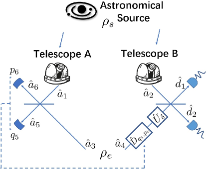
Figure 1: Setup for astronomical interferometry using continuous variable quantum teleportation. $\rho_{s}$ is the stellar state from the astronomical source and $\rho_{e}$ is the two-mode squeezed state. The dashed line indicates classical communication from telescope A to telescope B about the outcome $q_{5}$, $p_{6}$ of homodyne detection. $\hat{D}_{q_{5},p_{6}}$ is the displacement conditional on $q_{5}$, $p_{6}$. $\hat{U}_{\delta}$ is the phase delay added for the measurement of the teleported state.

3 Measurement on the teleported states

We now consider how well can we estimate the coherence function $g$ by measuring the nonideal teleported state. For the estimation of a set of parameters $\bm{z}=(\theta,|g|)^{T}$, the quantum Cramér-Rao bound (QCRB) [20] of estimating $\theta$ and $|g|$ is given by the quantum Fisher information (QFI) $F$: ${M_{\bm{z}}\geq F^{-1}}$, with its $(\mu,\nu)$ element ${[M_{\bm{z}}]_{\mu\nu}=\mathbb{E}\left[(\bm{z}_{\mu}-\check{\bm{z}}_{\mu})(\bm{z}_{\nu}-\check{\bm{z}}_{\nu})\right]}$, where $\check{\bm{z}}_{\mu}$ is the unbiased estimator of the $\mu$-th unknown parameter. QCRB is a fundamental bound of the sensitivity optimized over all possible measurements and estimators. We here calculate the QFI to quantify the performance of our scheme. For a Gaussian state, the QFI $F_{ij}$ can be derived from its mean value $x_{i}$ and covariance matrix $\Sigma$ ( $\Sigma=\frac{1}{2}\tr[\rho(\mathbf{a}_{i}\mathbf{a}_{j}+\mathbf{a}_{j}\mathbf{a}_{i})]$ is an equivalent form of covariance matrix $V$, where $\mathbf{a}=[a_{1},a_{1}^{\dagger},a_{2},a_{2}^{\dagger}]$) [21, 22]:

$$F_{ij}=\frac{1}{2}\mathfrak{M}_{\alpha\beta,\mu\nu}^{-1}\partial_{j}\Sigma_{\alpha\beta}\partial_{i}\Sigma_{\mu\nu}+\Sigma_{\mu\nu}^{-1}\partial_{j}x_{\mu}\partial_{i}x_{\nu},$$ (11)

where ${\mathfrak{M}=\Sigma\otimes\Sigma+\frac{1}{4}\Omega\otimes\Omega}$, with ${\Omega=\bigoplus_{k=1}^{n}i\sigma_{y}}$ with $\sigma_{y}$ being the Pauli $y$ matrix, $\partial_{j}$ is the derivative over the $j$-th unknown parameter, and repeated indices imply summation. The QFI of estimating $\theta,|g|$ is derived as

$$F_{\theta\theta}=\frac{2\epsilon^{2}|g|^{2}}{2y+\epsilon(2+\epsilon-\epsilon|g|^{2}+2y)}$$ (12)

$$F_{|g||g|}=\frac{2\epsilon^{2}[-\epsilon(2+\epsilon)^{2}+\epsilon^{3}|g|^{4}-4(1+\epsilon)(2+\epsilon)y-4(2+\epsilon)y^{2}]}{[\epsilon(-1+|g|^{2})-2y][\epsilon(-2-\epsilon+\epsilon|g|^{2})-2(1+\epsilon)y][\epsilon^{2}(-1+|g|^{2})-4(1+y)-2\epsilon(2+y)]}$$

$$F_{\theta|g|}=0,$$

where $y=2e^{-2r^{\prime}}$. In the infinite squeezing limit $y\rightarrow 0$, the sensitivity is the same as the direct-detection method assuming no transmission loss. This is because $V^{\prime}=V$ in that case, which means we have brought the light from the two telescopes to the same location perfectly. If the squeezing level is not infinite, as shown in Fig. 2, as long as $y$ is comparable to $\epsilon$, we can already obtain reasonable sensitivity. Thus, we can use a squeeze source to do quantum teleportation and avoid transmission loss in the astronomical interferometer.

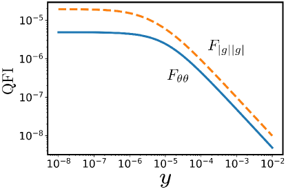
Figure 2: The quantum Fisher information (QFI) for estimating the phase $\theta$ and amplitude $|g|$ of the coherence function as a function of the squeezing level $y$. The parameters are chosen as $|g|=0.7$, $\epsilon=10^{-5}$.

We explicitly compare our scheme based on a CV quantum network with the scheme based on discrete-variable (DV) quantum networks proposed by Ref. [6] and heterodyne techniques by calculating the FI of estimating $\theta$. As shown in Fig. 3, as the mean photon number $\epsilon\rightarrow 0$, we observe the ratio between the FI of the CV and DV methods approach a constant of $1/2$. This factor of 1/2 is due to the fact that Ref. [6] wastes half of the stellar photons because it is not possible to implement the whole set of Bell measurements only using linear optics. In contrast, our scheme relies on homodyne detection instead and can be implemented with only linear optics. As $\epsilon$ increases, the performance gap between the schemes based on DV and CV quantum networks increases. This is because multiphoton events become more and more important as $\epsilon$ increases, and since our method makes use of the general stellar state with possibly more than one photon in Eq. 1, it can use multiphoton events instead of regarding them as noise as in Ref. [6, 7, 8]. However, as $\epsilon$ becomes large enough, it becomes possible to perform measurements locally without any entanglement resources or directly combining the light from two distant telescopes, as claimed in Ref. [5]. We calculate the performance of estimating $\theta$ only using heterodyne detection locally at each telescope. It is clear from the figure that for $\epsilon\gg 1$, local heterodyne detection without any entanglement can perform as well as our scheme based on a CV quantum network for the estimation of phase $\theta$. This shows that there exist schemes that only do measurement locally without any entanglement and still have the optimal performance for imaging strong thermal sources using interferometry with two telescopes. For intermediate values of $\epsilon$, our method can perform significantly better than methods based on DV quantum networks and local heterodyne detection.

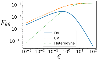
Figure 3: The Fisher information (FI) for estimating the phase $\theta$ of the coherence function by discrete variable (DV) quantum-network-based astronomical interferometry, continuous variable (CV) quantum-network-based astronomical interferometry, and local heterodyne detection, as a function of the mean photon number per temporal mode of the stellar light $\epsilon$.

Although our scheme works for sources of arbitrary strength, it is important to check its performance in the weak limit $\epsilon\ll 1$. This is because in the weak limit, the estimation of the coherence function is strongly affected by vacuum noise, which degrades sensitivity if there is no shared entanglement between the two telescopes and only local measurements are performed at each telescope, as pointed out in Ref. [5]. We quantify the performance using the Fisher information (FI), which is defined for a particular type of measurement and also bounds $\Sigma_{\bm{z}}$ by its inverse [20]. Reference [5] shows a local scheme without entanglement will at most have FI $F\propto\epsilon^{2}$. We now compare the FI of such a local scheme with the QFI of our scheme, which teleports the stellar state using entanglement, to show our scheme overcomes the vacuum noise. In the weak limit, the QFI of our scheme is

$$F_{\theta\theta}\xrightarrow[]{y\ll\epsilon\ll 1}\epsilon|g|^{2},$$ (13)

$$F_{|g||g|}\xrightarrow[]{y\ll\epsilon\ll 1}\frac{\epsilon}{1-|g|^{2}},$$

which shows our scheme has $F\propto\epsilon$. Since $\epsilon\ll 1$ and the inverse of $F$ is the lower bound for the variance of the estimation, we find that our scheme can significantly outperform local schemes without entanglement. In addition, the QFI we find here is comparable to that of schemes in Ref. [6, 7, 8], where different types of entanglement resources are used.

We now consider the positive operator-valued measure (POVM) that can saturate the sensitivity predicted by the QFI. The optimal POVM can be found from the eigenbasis of the symmetric logarithmic derivative (SLD) [23, 24]. Since the teleported state is a Gaussian state, we can determine the SLD as a function of mean value $x_{i}$ and covariance matrix $\Sigma$ [21, 22] as follows:

$$\mathcal{L}_{i}=\frac{1}{2}\mathfrak{M}_{\gamma\kappa,\alpha\beta}^{-1}\left(\partial_{i}\Sigma_{\alpha\beta}\right)\left(\mathbf{a}_{\gamma}\mathbf{a}_{\kappa}-\Sigma_{\gamma\kappa}\right),$$ (14)

where we sum over repeated indices. For the estimation of $|g|$, the SLD is

$$\mathcal{L}_{|g|} =\frac{a}{d}(2\hat{a}_{4}^{\dagger}\hat{a}_{4}+1)+\frac{c}{d}(2\hat{a}_{2}^{\dagger}\hat{a}_{2}+1)$$ (15)

$$\quad\quad+\frac{2b}{d}\hat{a}_{4}\hat{a}_{2}^{\dagger}+\frac{2b^{*}}{d}\hat{a}_{4}^{\dagger}\hat{a}_{2}+e,$$

$$a=2\epsilon^{2}|g|[-(1+\epsilon)(-2+\epsilon(-1+|g|^{2}))$$ (16)

$$\quad\quad\quad\quad\quad\quad+2(2+\epsilon)y],$$

$$b=\epsilon e^{-i\theta}[-\epsilon(2+\epsilon)^{2}+\epsilon^{3}|g|^{4}$$

$$\quad\quad\quad-4(1+\epsilon)(2+\epsilon)y-4(2+\epsilon)y^{2}],$$

$$c=2\epsilon^{2}|g|[-\epsilon(1+\epsilon)(-2+\epsilon(-1+|g|^{2}))$$

$$\quad\quad+2y(2+\epsilon(4-\epsilon(-2+|g|^{2})))+4(1+\epsilon)y^{2}],$$

$$d=[\epsilon(-2+\epsilon(-1+|g|^{2}))-2(1+\epsilon)y]$$

$$\quad\quad\times[\epsilon^{2}(-1+|g|^{2})-4(1+y)-2\epsilon(2+y)]$$

$$\quad\quad\times[\epsilon(-1+|g|^{2})-2y],$$

$$e=-\epsilon|g|\bigg{[}\frac{1}{\epsilon(-1+|g|^{2})-2y}$$

$$\quad\quad\quad+\frac{\epsilon}{\epsilon^{2}(-1+|g|^{2})-4(1+y)-2\epsilon(2+y)}\bigg{]}.$$

To find its eigenbasis, we define $\hat{d}_{1}=(\hat{a}_{4}+e^{i\delta}\hat{a}_{2})/\sqrt{2}$, $\hat{d}_{2}=(\hat{a}_{4}-e^{i\delta}\hat{a}_{2})/\sqrt{2}$:

$$\mathcal{L}_{|g|} =\hat{d}_{1}^{\dagger}\hat{d}_{1}(a+c+be^{i\delta}+b^{*}e^{-i\delta})/d$$ (17)

$$\quad\quad+\hat{d}_{2}^{\dagger}\hat{d}_{2}(a+c-be^{i\delta}-b^{*}e^{-i\delta})/d$$

$$\quad\quad+e+\frac{a+c}{d}$$

$$\quad\quad+\hat{d}_{1}^{\dagger}\hat{d}_{2}(a-c+be^{i\delta}-b^{*}e^{-i\delta})/d$$

$$\quad\quad+\hat{d}_{2}^{\dagger}\hat{d}_{1}(a-c-be^{i\delta}+b^{*}e^{-i\delta})/d.$$

We want to choose $\delta$ such that $(a-c+be^{i\delta}-b^{*}e^{-i\delta})/d=(a-c-be^{i\delta}+b^{*}e^{-i\delta})/d=0$, which implies the eigenbasis is the Fock basis of $d_{1,2}$ modes. If $y\ll 1$ and $y\ll\epsilon$, to the leading order of $y$, we have

$$(a-c+be^{i\delta}-b^{*}e^{-i\delta})/d$$ (18)

$$=-(a-c-be^{i\delta}+b^{*}e^{-i\delta})/d$$

$$=\frac{2i\sin(\delta-\theta)(2+\epsilon+\epsilon|g|^{2})}{(-1+|g|^{2})[-4-4\epsilon+\epsilon^{2}(-1+|g|^{2})]}+o(1).$$

This means we can choose $\delta=\theta$ in the measurement, and the POVM is $\{\ket{m,n}\bra{m,n}\}_{m,n}$, where $d_{1}^{\dagger}d_{1}\ket{m,n}=m\ket{m,n}$ and $d_{2}^{\dagger}d_{2}\ket{m,n}=n\ket{m,n}$. This measurement can be implemented using beam-splitters and photon-number-resolving detection with phase delay $\delta=\theta$, as shown in Fig. 1.

For the estimation of phase $\theta$, the SLD is given by

$$\mathcal{L}_{\theta} =2p^{*}a_{4}a_{2}^{\dagger}+2pa_{4}^{\dagger}a_{2},$$ (19)

$$p=\frac{i\epsilon g}{-\epsilon[-2+\epsilon(-1+|g|^{2})]+2(1+\epsilon)y}.$$ (20)

To find its eigenbasis, we define $d_{1}=(a_{4}+e^{i\delta}a_{2})/\sqrt{2}$, $d_{2}=(a_{4}-e^{i\delta}a_{2})/\sqrt{2}$,

$$\mathcal{L}_{\theta} =d_{1}^{\dagger}d_{1}(p^{*}e^{i\delta}+pe^{-i\delta})-d_{2}^{\dagger}d_{2}(p^{*}e^{i\delta}+pe^{-i\delta})$$ (21)

$$+d_{1}^{\dagger}d_{2}(p^{*}e^{i\delta}-pe^{-i\delta})+d_{2}^{\dagger}d_{1}(-p^{*}e^{i\delta}+pe^{-i\delta}).$$

To have $(p^{*}e^{i\delta}-pe^{-i\delta})=0$, we can choose $\delta=\theta+\pi/2$. And the POVM is $\{\ket{m,n}\bra{m,n}\}_{m,n}$, where $d_{1}^{\dagger}d_{1}\ket{m,n}=m\ket{m,n}$ and $d_{2}^{\dagger}d_{2}\ket{m,n}=n\ket{m,n}$ (with a different $\delta$ when compared with the estimation of $|g|$). This POVM can be also implemented using beam-splitters and photon-number-resolving detection as in Fig. 1 with phase delay $\delta=\theta+\pi/2$.

Since in the limit $y\ll\epsilon$, we can expect the teleported light to be the same as the state after directly bringing the light together to one location losslessly, the classical measurement schemes developed in astronomy should work as usual. For example, if we just measure the intensity difference between the two output ports $d_{1,2}$ with observable $\hat{O}=(d_{1}^{\dagger}d_{1}-d_{2}^{\dagger}d_{2})/(2\epsilon)$, we have $\langle\hat{O}\rangle=|g|\cos(\theta-\delta)$ and the variance $\langle\hat{O}^{2}\rangle-\langle\hat{O}\rangle^{2}$ is given by $[\epsilon+y+\epsilon(\epsilon/2+y)-\epsilon^{2}|g|^{2}/2+\epsilon^{2}|g|^{2}\cos^{2}(\theta-\delta)]/\epsilon^{2}$, which is comparable to the performance predicted by the QFI. Note that we do not need to know the squeezing parameter $r$ to estimate the coherence function and this estimator is unbiased even if the squeezing level is finite or even lower than the threshold. Intuitively, when $y$ is finite, there is background noise introduced by $y$ for the intensity measured at $d_{1,2}$, which is canceled when we take the difference between the intensities at $d_{1,2}$.

Furthermore, since $\theta$ is an unknown parameter, it is in general not possible to implement the optimal measurement strategy for the estimation of $\theta$ and $|g|$. We can certainly do the measurement adaptively and gradually optimize the phase in practice. We here want to briefly discuss the influence of having a phase delay in our measurement deviating from the optimal values. For simplicity, we assume $y\ll\epsilon\ll 1$. And we again consider the measurement that interferes with the light after adding the phase delay $\delta$ just as in Fig. 1. The FI of estimating $\theta$ and $g$ using this measurement to the leading order of $\epsilon$ is

$$I_{\theta\theta}=\epsilon\frac{|g|^{2}\sin^{2}(\theta-\delta)}{1-|g|^{2}\cos^{2}(\theta-\delta)},$$ (22)

$$I_{|g||g|}=\epsilon\frac{\cos^{2}(\theta-\delta)}{1-|g|^{2}\cos^{2}(\theta-\delta)},$$

$$I_{\theta|g|}=-\epsilon\frac{|g|\sin(\theta-\delta)\cos(\theta-\delta)}{1-|g|^{2}\cos^{2}(\theta-\delta)}.$$

If we focus on scenarios where the size of the source exceeds the resolution limit and the intensity distribution becomes more complex than simple point sources, it is highly probable that $|g|\ll 1$. This is because the parameter $g$ represents a weighted sum of various phases. When these weights approach a more uniform or flat distribution, $g$ tends to approach 0. So, the performance is mainly determined by the numerator of the FI in Eq. 22. We observe that the performance indeed decreases if $\delta$ deviates from the optimal values $\delta=\theta$, $\theta+\pi/2$ for estimation of $\theta$ and $|g|$, respectively. But reasonable performance can still be achieved as long as the deviation is not too large.

4 Amplification of entanglement resources

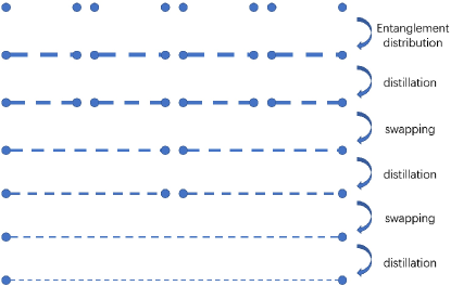
Figure 4: Continuous-variable quantum repeater. The two-mode squeezed states are distributed to adjacent quantum nodes through lossy channels. After several rounds of entanglement distillation and entanglement swapping, we create entanglement over a long distance. The blue circles are quantum nodes. The dashed line indicates entanglement and the thickness indicates the number of copies. The states are stored in quantum memories in each quantum node until their use.

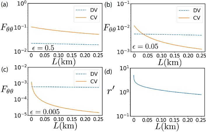
Figure 5: Influence of transmission loss on interferometric imaging based on discrete-variable (DV) and continuous-variable (CV) schemes when there is no entanglement distillation or quantum repeaters. We assume the transmission loss is 0.2 dB/km. (a-c) The Fisher information $F_{\theta\theta}$ of estimating the phase $\theta$ of the coherence function versus the baseline between telescopes $L$, for the mean photon number per temporal mode $\epsilon=0.5,0.05,0.005$. For the CV case, we assume the squeezing parameter $r=5$ before the two-mode squeezed state is sent through the lossy channel. (d) The effective squeezing parameter $r^{\prime}$ decreases with the baseline $L$.

We first explore for both DV and CV cases the situation where entanglement resources are distributed without any entanglement distillation or quantum repeaters. As shown in Fig. 5, we consider the FI of estimating the phase of the coherence function versus the baseline length $L$ for different strengths $\epsilon$ of the stellar source. The FI for the DV case decays exponentially with $L$ because loss increases for the terrestrial photons, resulting in a higher probability for vacuum state contributions. The behavior of the FI as a function of $L$ in the CV cases depends on the source strength $\epsilon$. This is because the value of the effective squeezing parameter $r^{\prime}$ at which the QFI starts to significantly drop depends on $\epsilon$. This can be seen from Fig. 2 and Eq. LABEL:FI, which show $y=2e^{-2r^{\prime}}$ should be at least comparable to $\epsilon$ to obtain sensitivity close to the optimal case when $y\rightarrow 0$. To make $r^{\prime}$ comparable to $r$, the effective transmission coefficient $T$ needs to satisfy $1-T^{2}\sim e^{-2r}$. Given a squeezing parameter $r$ high enough such that the QFI approaches its optimal value, to keep reasonable performance $1-T^{2}$ should be at least comparable to $\epsilon$. When $\epsilon$ is small, the requirement on $T$ is very high and the performance of our scheme based on CV teleportation decays very fast. When $\epsilon\sim O(1)$, our scheme based on CV teleportation becomes more robust to loss.

An important question is how to achieve in practice a high-fidelity two-mode squeezed state shared by distant telescopes connected by lossy quantum channels. As discussed in the previous section, a lossy squeezed state will strongly limit the sensitivity. As in the discrete case [6] where one must build shared entanglement between distant telescopes with a DV quantum repeater, we will need to apply the CV quantum repeater to the problem of creating long-baseline astronomical interferometers [25, 26, 27, 28, 29, 30, 31]. This will allow us to extend the baseline of interferometers beyond what is possible to achieve by direct interference.

As shown in Fig. 4, in the network of a CV quantum repeater, repeater nodes are located at a modest distance between each other. The first step to connect adjacent telescopes is to distribute two-mode squeezed states between adjacent nodes and perform entanglement distillation, which can generate a smaller number of two-mode squeezed states with less noise from more noisy two-mode squeezed states. Then, entanglement swapping joins together multiple entangled states and creates entangled states between arbitrarily distant stations [27, 28, 30, 31]. The CV quantum repeater can help us reduce two types of noise. The first type is the phase noise caused by the variation of the path length of the interferometer. This can be solved by active stabilization [32], where the distance is tracked by a reference laser. Or the phase noise can be overcome by entanglement distillation [29]. The second type of noise is transmission loss. Entanglement distillation can also create entanglement between adjacent nodes with better effective transmissivity $\eta$ and squeezing level $r$ compared to using a directly transmitted entangled state [25, 26]. More details on building CV quantum repeaters based on entanglement distillation and entanglement swapping can be found in Appendix A.

For the purpose of imaging, the parameters relevant to performance are squeezing level $r$, transmission loss in the distribution of entanglement $T$, and repetition rate. A CV quantum repeater can ensure transmission loss is limited to a small constant over long distances [27], which suggests a fixed $T$ in the output of the repeater. Recall that we have defined effective squeezing level $r^{\prime}$ such that $e^{-2r^{\prime}}=1-T^{2}+e^{-2r}T^{2}$. As a simple model, we consider the case of fixing $r^{\prime}$ with the help of CV repeaters even when the distance increases. Then, the goal is to make sure $T$ is large enough so that $r^{\prime}$ can be comparable to $r$. The repetition rate of a quantum repeater depends on the rate of the sources at each repeater node and the success probability of quantum operations at each node, such as entanglement distillation and swapping. The repetition rate will be polynomial in the distance between two telescopes. If we consider the CV repeater proposed in Ref. [27], the transmission loss between nearby repeater nodes and the squeezing level will determine the order of the polynomial.

As the squeezing level and repetition rate of the quantum repeater become high enough, we can expect the quantum teleportation to be approximately ideal. If we choose $\lambda=800\;\text{nm}$, $\Delta\lambda=0.1\;\text{nm}$, the threshold for the repetition rate of our repeater to make sure our distributed two-mode squeezed states cover all the temporal modes is roughly 150 GHz. We assume the diameter of each telescope is 6 m. We list the threshold squeezing level for different magnitudes of stellar sources in Table 1. The current state of the art is up to 15 dB squeezing level can be expected from a squeezed light source [33, 34]. If we can distribute two-mode squeezed states with both the squeezing level and repetition rate better than their thresholds, our scheme can overcome the transmission loss and hence significantly outperform the direct detection case which suffers from the transmission loss. Since $\epsilon$ will determine the required squeezing level and very strong squeezing levels are required to image weak sources, it may be advantageous to increase the mean photon number per temporal mode by having more than two telescopes work together in this scheme while imaging weak sources. But this scheme would require a modified version of the standard CV quantum teleportation, which is left as a possible future direction of work.

We explicitly compare the performance of our scheme and the method of directly combining the light from two distant telescopes in Fig. 6. We choose a relatively strong stellar source of magnitude -5, because when $\epsilon\sim O(1)$, our scheme can show advantage over both the DV scheme in Ref. [6] and local heterodyne detection as discussed previously in relation to Fig. 3. For an astronomical source of magnitude -5 imaged with telescopes of diameter 6 m at $\lambda=800\;\text{nm}$, $\Delta\lambda=0.1\text{nm}$, the mean photon number per temporal mode is roughly $\epsilon\sim 0.4$. This is also the regime in which the requirement for effective squeezing is not so high, with the threshold for the effective squeezing parameter $r^{\prime}$ roughly $0.8$. The required repetition rate to cover all the temporal modes is roughly 150 GHz. We consider a range of values of $r^{\prime}$ and repetition rate for quantum repeaters operating at a distance of 10 km. For longer distances, we include the polynomial decrease of repetition rate as distance becomes longer while fixing $r^{\prime}$ as a constant [27]. In practice, this can be achieved by entanglement distillation, which consumes multiple copies of the noisy two-mode squeezed states and generates two-mode squeezed states with larger effective squeezing parameter $r^{\prime}$, as detailed in Appendix A. As shown in Fig. 6, even if the required repetition rate and squeezing values are not achieved, as distance lengthens, our scheme is still preferable.

Table 1: Threshold of squeezing level for different magnitude of stellar sources with $\lambda=800\text{nm}$, $\Delta\lambda=0.1\text{nm}$.

Magnitude	$\epsilon$	Squeezing (dB)	$r^{\prime}$
-5	$4\times 10^{-1}$	7	0.80
-2.5	$4\times 10^{-2}$	17	1.96
0	$4\times 10^{-3}$	27	3.11
2.5	$4\times 10^{-4}$	37	4.26
5	$4\times 10^{-5}$	47	5.41
7.5	$4\times 10^{-6}$	57	6.56

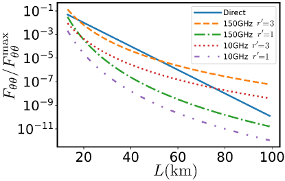
Figure 6: Ratio of achieved FI over the maximum FI in the ideal case for estimating the phase of the coherence function $\theta$. The solid blue line corresponds to the case of directly combining the light from telescopes with baseline $L$ in units of kilometers. We assume the transmission loss is 1 dB/km. The other plotted lines are the performance of our CV quantum-network-based scheme for different repetition rates and effective squeezing parameters $r^{\prime}$. Here we assume the quantum repeater operates with the chosen repetition rate at a distance of 10 km, and that the repetition rate starts to decrease polynomially with distances larger than 10 km. We assume $\lambda=800\;\text{nm}$, $\Delta\lambda=0.1\;\text{nm}$, the source has magnitude -5, and we are using telescopes of diameter 6 m.

We previously compared our scheme based on CV quantum repeaters with the scheme based on DV quantum repeaters proposed in Ref. [6] in Fig. 3, assuming the repeaters are ideal. But the real-world implementation of CV and DV quantum repeaters will obviously affect the imaging quality of the two schemes. As the preliminary proposal for CV quantum repeaters appeared only recently [27], and the development of CV quantum repeaters is still in its early stages, it is hard for us to predict which scheme will eventually show better performance. We note there are some theoretical efforts on the direct comparison between DV and CV quantum repeaters [35]. They consider the ability to distribute a two-mode squeezed vacuum as the figure of merit to compare DV and CV repeaters. Their results suggest that CV repeaters may outperform DV repeaters for a certain fidelity of DV entangled pairs. Although this work suggests an inspiring way to benchmark the two different approaches and suggests that CV repeaters may outperform DV repeaters in some parameter regimes, their comparison relies on several assumptions, such as using DV entanglement to distribute CV entanglement and the strength of the two-mode squeezed vacuum. The comparison between our scheme and Ref. [6] in actual implementation requires more theoretical and experimental effort and is left as future work.

We now compare our method with the intensity interferometer [36] and heterodyne interferometer [37]. The intensity interferometer measures the intensity fluctuations at two distant telescopes independently as a function of time, which is then used to find the second-order correlation of the received light via data post-processing [36]. For thermal light, the second-order correlation function is directly related to the coherence function we want to measure. Compared to our method, the intensity interferometer is much easier to implement since the measurement is independent in each telescope. But for weak thermal sources, the intensity interferometer has much worse sensitivity because it requires at least two photons within the same temporal mode to extract useful information, meaning many temporal modes with one photon are wasted. Heterodyne detection mixes the light from the astronomical source with a laser on a beam-splitter in order to measure the coherence function [37]. Although the length of the baseline will be limited due to the optical feedback system used for phase-locking lasers at the two telescopes, this is still much easier than distributing fragile entangled states. However, the sensitivity is once again worse than our method for weak sources. This is mainly because local heterodyne detection is unable to distinguish the vacuum state and states with at least one photon in the stellar light while measuring the coherence function, which introduces strong vacuum noise to the estimation, as pointed out in Ref. [5].

In gravitational wave detectors, which represent an important application of squeezed states, photon counting noise can be reduced by injecting the squeezed state into one port of the interferometer [38]. A natural question is whether we can enhance the estimation of coherence using squeezed light instead of only using squeezed states as entanglement resources to perform quantum teleportation. The answer is unfortunately no. Intuitively, this is because in the gravitational wave detector [38], the squeezed state is also encoded with the unknown phase we want to estimate, i.e. the squeezed state can be regarded as part of the probe state. But for astronomical interferometers, the state we receive at the telescopes is already encoded with the information we want to measure. The squeezed state can only be used in ancillary modes and not as a probe state. More details can be found in Appendix B.

5 Conclusion

In summary, we propose to use two-mode squeezed states as an entanglement resource to overcome transmission loss in astronomical interferometry. Our scheme is based on the CV teleportation of stellar light. The optimal measurement on the teleported states to estimate the coherence function is constructed using beam-splitters and photon-number-resolved detection. Due to phase noise and transmission loss in the distribution of the two-mode squeezed states, our scheme relies on CV quantum repeaters to build entanglement between distant telescopes.

6 Acknowledgements

We would like to thank Eric Chitambar, Andrew Jordan, Paul Kwiat, John D. Monnier, Shayan Mookherjea, Michael G. Raymer and Brian J. Smith for helpful discussion. This work was supported by the multi-university National Science Foundation Grant No. 1936321 – QII-TAQS: Quantum-Enhanced Telescopy.

Appendix A Continuous variable quantum repeaters

In the basic CV quantum repeater, many copies of two-mode squeezed states are distributed to adjacent repeater nodes. As shown in Fig. 4, each repeater node then does entanglement distillation and entanglement swapping [27, 28, 30, 31]. There are several types of entanglement distillation and swapping methods. We now introduce some representatives of them.

One entanglement distillation method for overcoming transmission loss is based on noiseless linear amplification [25, 26]. Consider the distribution of two-mode squeezed states with squeezing parameter $r$ through a channel with transmissivity $\eta$. For the transmitted state, we split the quantum state into $N$ modes using a balanced beam-splitter. For each mode, we apply the quantum scissor operation [39, 40], which uses linear optics and single-photon detection. Conditioned on the outcome of the single photon detector, we can truncate the state into the subspace spanned by the Fock basis $\{\ket{0}$, $\ket{1}\}$ and amplify the coefficient of $\ket{1}$ at the same time. We then recombine all the modes into one mode using a beam-splitter. Postselecting on detecting vacuum in all but one output port, we can get an amplified two-mode squeezed state with a better squeezing level $r_{\text{eff}}$ and larger transmissivity $\eta_{\text{eff}}$ at the cost of losing the states when we do not get the expected measurement outcomes. This allows us to distill the entanglement between distant nodes so that we can obtain highly entangled states even under the influence of transmission loss. Other entanglement distillation methods for overcoming transmission loss include symmetric photon replacement [41] and purifying distillation [42]. The outcome of the entanglement distillation is in general no longer a Gaussian state since we perform a non-Gaussian operation, which should be supported by Gaussification protocols [43, 44].

Entanglement distillation dealing with phase noise can be implemented with quantum memories whose memory processes are beam-splitter-like operations and balanced homodyne detection on the transmitted optical modes [29]. Optical two-mode squeezed states are distributed to distant quantum nodes, during which process they suffer from phase noise. The optical states are transferred to the quantum memories at each node. A second optical two-mode squeezed state is distributed and interfered with the state of the quantum memories in the memory process, which is a beam-splitter-like operation. Conditioned on the outcome of homodyne detection on the transmitted optical mode of the beam-splitter-like operation, the entanglement is distilled. This entanglement distillation method provides highly entangled states for downstream applications under random phase fluctuations in the quantum channels used for distribution of the entangled states.

Entanglement swapping can be a Gaussian operation [45], which mixes the two modes at the same node on a balanced beam-splitter and does homodyne detection at the output ports. The outcomes are then used at the two other nodes for the corresponding correction operation by displacing the states. Entanglement swapping can also be a non-Gaussian operation [28], in which one basically swaps the entanglement in the low-photon-number subspace. This non-Gaussian swapping protocol will of course require further Gaussification.

As an attractive alternative to DV schemes, CV systems are also compatible with existing optical telecom systems. But in contrast to the well-developed DV quantum repeater [9], CV quantum repeaters are still in their infancy. Many existing proposals for CV quantum repeaters are similar to first-generation DV quantum repeaters, which require two-way classical communication beyond the nearest nodes [27, 28, 30]. Some efforts have been made to develop second-generation CV repeaters which only require nearest-neighbor two-way classical communication [31] and third-generation CV quantum repeaters which do not need two-way classical communication and are completely one-way [46]. Currently, CV quantum repeaters certainly cannot work at the repetition rates required in astronomical interferometry. We might expect a large gain in the performance once second- and third-generation CV quantum repeaters are well established, which requires the development of CV error correction codes.

Appendix B Photon counting noise in the presence of squeezed states

A famous application for squeezed states is in the interferometer used for gravitational wave detection [38]. Squeezed states are used as a resource to reduce photon counting noise at the expense of increasing the fluctuation of radiation pressure, which is useful when the optimal laser power is not available in the practical implementation. Since our method involves squeezed states, there is a natural question: if we assume the ideal implementation of the measurement and ignore the transmission loss, which is the reason we want to use quantum teleportation instead of directly bringing the light from two telescopes to one location, can we fundamentally enhance the estimation of the coherence function over the conventional method? To the best of our understanding, the answer is unfortunately no. A short explanation is that if we consider the estimation of the coherence function using quantum estimation theory as discussed in Ref. [47], the fundamental sensitivity limit is given by the QFI. And the measurement that can saturate the optimal sensitivity for the estimation of the phase and amplitude of the coherence function can be constructed using beam-splitters and photon-number-resolved detection, respectively. The sensitivity bound given by the QFI has been optimized over all possible measurements that are physically allowed, which of course includes schemes that use squeezed states as ancilla. So, we should not expect using squeezed states to enhance the sensitivity of the astronomical interferometer. Compared with gravitational wave detection [38], the main difference is that in gravitational wave detection, the squeezed state is also used as an input state that is encoded with the information to measure. And in the case of the astronomical interferometer, we cannot change the state received by the astronomical source.

To gain more intuition, we consider an interferometer used for phase estimation enhanced by squeezed states, which can be regarded as a simplified version of the discussion in [38], where we are removing all discussions related to radiation pressure. The setup is shown in Fig. 7. As we will see, the squeezed state in the second port of the beam-splitter can reduce the noise in the estimation when compared with the case where we leave the $a_{2}$ mode as the vacuum state. The unknown phase $\phi$ is estimated from the mean value of $n=c_{1}^{\dagger}c_{1}-c_{2}^{\dagger}c_{2}$ and its noise is quantified by the variance of $n$:

$$\langle n\rangle=(\sinh^{2}r-|\alpha|^{2})\cos\phi,$$ (23)

$$\langle\Delta n^{2}\rangle=\cos^{2}\phi(\alpha^{2}+2\sinh^{2}r\cosh^{2}r)$$

$$\quad\quad\quad\quad+\sin^{2}\phi(\alpha^{2}\cosh 2r+\sinh^{2}r),$$

where $\langle.\rangle$ is the mean value of the operators for the quantum state in the output ports of the beam-splitter and we have assumed $\alpha$ is real for simplicity. Following the discussion of photon-counting error in Ref. [38], we can consider $\phi$ such that $\cos\phi$ is close to zero. In this case, if we further assume the coherent state is much stronger than the squeezed state, the noise is dominated by $\sin^{2}\phi\alpha^{2}e^{2r}/2$, which can be reduced by $r<0$. Now we consider whether this method can be applied to the astronomical interferometer. Note the squeezed state is used as the input of the interferometer. This is not possible for an astronomical interferometer since the unknown phase is only encoded in the received thermal state and the squeezed state can only be used as the ancilla of implementing the measurement.

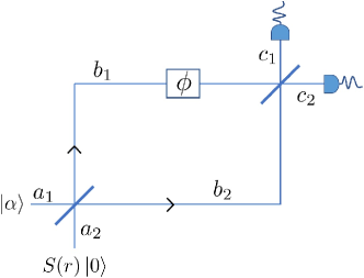
Figure 7: An interferometer used for phase estimation enhanced by squeezed states. The two input ports $a_{1,2}$ are in coherent state $\ket{\alpha}$ and squeezed state $S(r)\ket{0}=\exp(\frac{r}{2}a_{2}^{2}-\frac{r}{2}{a_{2}^{\dagger}}^{2})\ket{0}$. In one arm of the interferometer, an unknown phase $\phi$ is encoded on the state by unitary transformation $U(\phi)=\exp(\phi b_{1}^{\dagger}b_{1})$. We measure the observable $n=c_{1}^{\dagger}c_{1}-c_{2}^{\dagger}c_{2}$ to estimate $\phi$.

Another intuitive question is whether we can use the squeezed LO in the implementation of the measurement. If we consider the implementation of heterodyne detection, in the large LO power limit, the LO noise makes no contribution to the total noise of the measurement results [48]. So, it is not meaningful to use squeezed light as the LO because reducing the LO noise cannot reduce the noise of the measurement, at least in any obvious way. There are some discussions that try to improve heterodyne detection using squeezed states such as Ref. [49], which however has invited debate [50, 51]. So, we are satisfied with the answer that squeezed states can only be used as entanglement resources to overcome transmission loss and will not fundamentally enhance the estimation of coherence functions in an obvious way.

References

- [1] Frederik Zernike. The concept of degree of coherence and its application to optical problems. Physica, 5(8):785–795, 1938.
- [2] Event Horizon Telescope Collaboration, First m87 event horizon telescope results. i. the shadow of the supermassive black hole. Astrophys. J. Lett, 875(1):L1, 2019.
- [3] Thomas L Wilson, Kristen Rohlfs, and Susanne Hüttemeister. Tools of radio astronomy, volume 5. Springer, 2009.
- [4] John D Monnier. Optical interferometry in astronomy. Reports on Progress in Physics, 66(5):789, 2003.
- [5] Mankei Tsang. Quantum nonlocality in weak-thermal-light interferometry. Physical review letters, 107(27):270402, 2011.
- [6] Daniel Gottesman, Thomas Jennewein, and Sarah Croke. Longer-baseline telescopes using quantum repeaters. Physical review letters, 109(7):070503, 2012.
- [7] Emil T Khabiboulline, Johannes Borregaard, Kristiaan De Greve, and Mikhail D Lukin. Optical interferometry with quantum networks. Physical review letters, 123(7):070504, 2019.
- [8] Emil T Khabiboulline, Johannes Borregaard, Kristiaan De Greve, and Mikhail D Lukin. Quantum-assisted telescope arrays. Physical Review A, 100(2):022316, 2019.
- [9] Nicolas Sangouard, Christoph Simon, Hugues De Riedmatten, and Nicolas Gisin. Quantum repeaters based on atomic ensembles and linear optics. Reviews of Modern Physics, 83(1):33, 2011.
- [10] Lev Vaidman. Teleportation of quantum states. Physical Review A, 49(2):1473, 1994.
- [11] Samuel L Braunstein and H Jeff Kimble. Teleportation of continuous quantum variables. Physical Review Letters, 80(4):869, 1998.
- [12] Stefano Pirandola and Stefano Mancini. Quantum teleportation with continuous variables: A survey. Laser Physics, 16(10):1418–1438, 2006.
- [13] Christian Weedbrook, Stefano Pirandola, Raúl García-Patrón, Nicolas J Cerf, Timothy C Ralph, Jeffrey H Shapiro, and Seth Lloyd. Gaussian quantum information. Reviews of Modern Physics, 84(2):621, 2012.
- [14] Jorge Amari, Junnosuke Takai, and Takuya Hirano. Highly efficient measurement of optical quadrature squeezing using a spatial light modulator controlled by machine learning. Optics Continuum, 2(4):933–941, 2023.
- [15] Leonard Mandel and Emil Wolf. Optical coherence and quantum optics. Cambridge university press, 1995.
- [16] Lu-Ming Duan and Guang-Can Guo. Influence of noise on the fidelity and the entanglement fidelity of states. Quantum and Semiclassical Optics: Journal of the European Optical Society Part B, 9(6):953, 1997.
- [17] AV Chizhov, E Schmidt, L Knöll, and DG Welsch. Propagation of entangled light pulses through dispersing and absorbing channels. Journal of Optics B: Quantum and Semiclassical Optics, 3(3):77, 2001.
- [18] Stefan Scheel, Tomas Opatrny, and D-G Welsch. Entanglement degradation of a two-mode squeezed vacuum in absorbing and amplifying optical fibers. Optics and Spectroscopy, 91(3):411–417, 2001.
- [19] AV Chizhov, L Knöll, and D-G Welsch. Continuous-variable quantum teleportation through lossy channels. Physical Review A, 65(2):022310, 2002.
- [20] CW Helstrom. Quantum detection and estimation theory, 123 academic press. New York, 1976.
- [21] Alex Monras. Phase space formalism for quantum estimation of gaussian states. arXiv preprint arXiv:1303.3682, 2013.
- [22] Yang Gao and Hwang Lee. Bounds on quantum multiple-parameter estimation with gaussian state. The European Physical Journal D, 68(11):1–7, 2014.
- [23] Samuel L Braunstein and Carlton M Caves. Statistical distance and the geometry of quantum states. Physical Review Letters, 72(22):3439, 1994.
- [24] Matteo GA Paris. Quantum estimation for quantum technology. International Journal of Quantum Information, 7(supp01):125–137, 2009.
- [25] TC Ralph and AP Lund. Nondeterministic noiseless linear amplification of quantum systems. In AIP Conference Proceedings, volume 1110, pages 155–160. American Institute of Physics, 2009.
- [26] TC Ralph. Quantum error correction of continuous-variable states against gaussian noise. Physical Review A, 84(2):022339, 2011.
- [27] Josephine Dias and Timothy C Ralph. Quantum repeaters using continuous-variable teleportation. Physical Review A, 95(2):022312, 2017.
- [28] Fabian Furrer and William J Munro. Repeaters for continuous-variable quantum communication. Physical Review A, 98(3):032335, 2018.
- [29] Yanhong Liu, Jieli Yan, Lixia Ma, Zhihui Yan, and Xiaojun Jia. Continuous-variable entanglement distillation between remote quantum nodes. Physical Review A, 98(5):052308, 2018.
- [30] Josephine Dias, Matthew S Winnel, Nedasadat Hosseinidehaj, and Timothy C Ralph. Quantum repeater for continuous-variable entanglement distribution. Physical Review A, 102(5):052425, 2020.
- [31] Kaushik P Seshadreesan, Hari Krovi, and Saikat Guha. Continuous-variable quantum repeater based on quantum scissors and mode multiplexing. Physical Review Research, 2(1):013310, 2020.
- [32] Seth M Foreman, Kevin W Holman, Darren D Hudson, David J Jones, and Jun Ye. Remote transfer of ultrastable frequency references via fiber networks. Review of Scientific Instruments, 78(2):021101, 2007.
- [33] Ulrik L Andersen, Tobias Gehring, Christoph Marquardt, and Gerd Leuchs. 30 years of squeezed light generation. Physica Scripta, 91(5):053001, 2016.
- [34] Henning Vahlbruch, Moritz Mehmet, Karsten Danzmann, and Roman Schnabel. Detection of 15 db squeezed states of light and their application for the absolute calibration of photoelectric quantum efficiency. Physical review letters, 117(11):110801, 2016.
- [35] Josephine Dias, Matthew S Winnel, William J Munro, TC Ralph, and Kae Nemoto. Distributing entanglement in first-generation discrete-and continuous-variable quantum repeaters. Physical Review A, 106(5):052604, 2022.
- [36] R Hanbury Brown and Richard Q Twiss. Correlation between photons in two coherent beams of light. Nature, 177(4497):27–29, 1956.
- [37] David DS Hale, M Bester, WC Danchi, W Fitelson, S Hoss, EA Lipman, JD Monnier, PG Tuthill, and CH Townes. The berkeley infrared spatial interferometer: a heterodyne stellar interferometer for the mid-infrared. The Astrophysical Journal, 537(2):998, 2000.
- [38] Carlton M Caves. Quantum-mechanical noise in an interferometer. Physical Review D, 23(8):1693, 1981.
- [39] Şahin Kaya Özdemir, Adam Miranowicz, Masato Koashi, and Nobuyuki Imoto. Quantum-scissors device for optical state truncation: A proposal for practical realization. Physical Review A, 64(6):063818, 2001.
- [40] David T Pegg, Lee S Phillips, and Stephen M Barnett. Optical state truncation by projection synthesis. Physical review letters, 81(8):1604, 1998.
- [41] AP Lund and TC Ralph. Continuous-variable entanglement distillation over a general lossy channel. Physical Review A, 80(3):032309, 2009.
- [42] Jaromír Fiurášek. Distillation and purification of symmetric entangled gaussian states. Physical Review A, 82(4):042331, 2010.
- [43] Daniel E Browne, Jens Eisert, Stefan Scheel, and Martin B Plenio. Driving non-gaussian to gaussian states with linear optics. Physical Review A, 67(6):062320, 2003.
- [44] J Eisert, DE Browne, S Scheel, and MB Plenio. Distillation of continuous-variable entanglement with optical means. Annals of Physics, 311(2):431–458, 2004.
- [45] Jason Hoelscher-Obermaier and Peter van Loock. Optimal gaussian entanglement swapping. Physical Review A, 83(1):012319, 2011.
- [46] Kosuke Fukui, Rafael N Alexander, and Peter van Loock. All-optical long-distance quantum communication with gottesman-kitaev-preskill qubits. Physical Review Research, 3(3):033118, 2021.
- [47] Mark E Pearce, Earl T Campbell, and Pieter Kok. Optimal quantum metrology of distant black bodies. Quantum, 1:21, 2017.
- [48] Horace P Yuen and Vincent WS Chan. Noise in homodyne and heterodyne detection. Optics letters, 8(3):177–179, 1983.
- [49] Yong-qing Li, Dorel Guzun, and Min Xiao. Sub-shot-noise-limited optical heterodyne detection using an amplitude-squeezed local oscillator. Physical review letters, 82(26):5225, 1999.
- [50] Yongqing Li, Dorel Guzun, and Min Xiao. Li, guzun, and xiao reply. Physical review letters, 85(3):678, 2000.
- [51] TC Ralph. Can signal-to-noise be improved by heterodyne detection using an amplitude squeezed local oscillator? Physical review letters, 85(3):677, 2000.