Abstract

Soft and collinear radiation in collider processes can be described in a universal way, that is independent of the underlying process. Recent years have seen a number of approaches for probing whether radiation beyond the leading soft approximation can also be systematically classified. In this paper, we study a formula that captures the leading next-to-soft QCD radiation affecting processes with both final- and initial-state partons, by shifting the momenta in the non-radiative squared amplitude. We first examine W+jet production, and show that a previously derived formula of this type indeed holds in the case in which massive colour singlet particles are present in the final state. Next, we develop a physical understanding of the momentum shifts, showing precisely how they disrupt the well-known angular ordering property of leading soft radiation.

1 Introduction

The calculation of scattering amplitudes in perturbative quantum field theory continues to be an area of intense activity, due to its many applications to current and future collider experiments. Whilst it is often possible to obtain complete amplitudes at a given order in the coupling constant, we sometimes wish to consider approximate results, particularly where these can be resummed to all orders in perturbation theory. A particularly well-studied case is the emission of soft and / or collinear radiation dressing an underlying scattering amplitude. This generates infrared singularities, which will cancel for suitably inclusive observables, such as total hadronic cross-sections. However, large contributions remain in perturbation theory, typically involving large logarithms of dimensionless energy ratios. A variety of methods have been developed for resumming such contributions (see e.g. refs. [1, 2, 3, 4, 5, 6, 7, 8, 9, 10, 11, 12, 13]), all of which rely on the tight relationship between kinematically enhanced terms and infrared singularities, plus the fact that soft and collinear factorisation can be described in terms of universal functions acting on arbitrary amplitudes. The latter property has a simple quantum mechanical interpretation: soft radiation has zero momentum, and thus an infinite Compton wavelength by the uncertainty principle. Thus, it cannot resolve the details of the underlying scattering amplitude that produced the hard outgoing particles. A similar story applies to collinear radiation, which instead has a zero transverse momentum relative to a given outgoing particle.

Heuristic arguments such as these are also useful for understanding the wider implications of soft radiation. Crucial for this paper will be a particular property of soft radiation that is emitted from pairs of (colour) charges, or dipoles, in QED or QCD. Including all possible quantum interference contributions in the squared amplitude, one finds in QED that radiation is confined to a cone around each charged particle, whose half-angle coincides with the angle between the two charged particle momenta. This is known as the Chudakov effect, and textbook treatments may be found in refs. [14, 15]. A corresponding effect holds in QCD, where for two colour charges there is no radiation (at leading soft level) outside the cones surrounding each particle. For more complicated configurations of partons, clusters of particles radiate according to their combined colour charge at sufficiently large angles. All of these phenomena have a common quantum mechanical origin similar to that already mentioned above: at large angles, the wavelength of the emitted radiation is such that it can only notice the combined colour charge of a given subset of partons. If this combined charge happens to be zero (or colour singlet in the QCD case), then there is no radiation at large angles.

So much for soft radiation, whose properties are already well-known. Until recently, much less has been known about how to systematically classify the properties of radiation at subleading order in a systematic expansion in the total radiated momentum. The frontier of such attempts is at next-to-leading power (NLP), and the last few years have seen an increasing number of techniques aimed at clarifying whether any universal statements can be made about such radiation, including its possible resummation. The range of methods [16, 17, 18, 19, 20, 21, 22, 23, 24, 25, 26, 27, 28, 29, 30, 31, 32, 33, 34, 35, 36, 37, 38, 39, 40, 41, 42, 43, 44, 45, 46, 47, 48, 49, 50, 51, 52, 53, 54, 55, 56, 57, 58, 59, 60, 61, 62, 63, 64, 65, 66, 67, 68, 69] – some of them inspired by the much earlier work of refs. [70, 71, 72] – mirrors that used for soft radiation, and this body of work is ultimately motivated by the fact that the numerical impact of such contributions may be needed to increase the theoretical precision of collider physics observables [73, 74, 75, 76, 77, 78, 79, 44]. As well as studies aiming to develop new resummation formulae, there is also scope for case studies that look at well-defined consequences of next-to-soft radiation, in order to build up our collective intuition of how it behaves. The aim of this paper is to carry out such a case study.

Our starting point is to consider a formula – first derived in ref. [31] and extended in ref [32] – that states that leading next-to-soft radiative contributions can be expressed in a particularly compact and elegant form. That is, the squared amplitude including such radiation can be written in terms of non-radiative amplitudes, but where distinct pairs of partonic momenta are shifted in a prescribed way. The shifted squared amplitudes are then dressed by overall factors which are identical to those that occur in the leading soft limit. Potential uses of such formulae include increasing the precision of numerical NLO calculations, and similar comments, independently and using different methods, have been made in refs. [57, 36, 37]. However, the obvious similarity of these momentum-shift formula to their leading-soft counterparts means they are an excellent starting point for examining the physics of next-to-soft radiation in a particularly transparent way.

In this paper, we will first review the momentum-shift formulae of refs. [31, 32], and introduce them by considering a process that has not previously been considered before in this approach. That is, we will consider radiative corrections to $W$ production in association with an additional hard jet. This is more general than either of the processes considered previously in this approach. Reference [31] looked only at colour-singlet final states, whereas ref. [32] considered only final states with massless particles. As we will yet again see, leading next-to-soft radiative corrections take the form of a series of dipole-like terms .

Next, we consider the effect of the momentum-shift formulae on the emission of soft radiation from a single final-state dipole. We will briefly review the well-known calculation of how soft gluon emission is confined to cones surrounding each hard particle, before correcting this to include the effects of the momentum-shifts, and hence leading next-to-soft effects. We will show explicitly that the next-to-soft corrections break the angular ordering property, in that they lead to emission outside of the usual angular region. That this property is not preserved beyond leading soft level will perhaps not surprise anyone. However, the mechanism by which this happens, including the details of the calculation, are interesting. Furthermore, given that the origin of the momentum shifts is well-understood as arising from orbital angular momentum effects [31, 32], we will be able to precisely interpret the physics of how angular ordering breaks down. We believe that this story offers novel insights into the physics of next-to-soft radiation that, as well as being compelling in themselves, may be of broader use.

The structure of our paper is as follows. In section 2, we examine $W$ + jet production at NLO, showing that the inclusion of radiative corrections up to next-to-soft level reproduces the same momentum-shift formula as was found for prompt production in ref. [32]. After drawing attention to the dipole-like nature of this formula, in section 3 we show that next-to-soft corrections lead to radiation outside the cone regions associated with leading soft radiation, and intepret the physics of this effect in detail. In section 4, we discuss our results and conclude.

2 A momentum-shift formula for $W$ plus jet production

2.1 $W$ plus jet production up to NLO

We start by considering the LO process

$$q(p_{1})+\bar{q}(p_{2})\rightarrow W(p_{3})+g(p_{4}),$$ (1)

whose Feynman diagrams are shown in figure 1. This is itself a correction to the Drell-Yan production of a $W$ boson, but we will consider that the final-state gluon is constrained to be hard (e.g. through a non-zero transverse momentum requirement), such that no infrared singularities are present. Our aim is to show how next-to-soft corrections to this process can be written according to a certain formula, and we will be able to illustrate our point without having to consider the alternative partonic channel $qg\rightarrow W+g$, which in any case can be obtained from crossing. Denoting the $W$ boson mass by $m$, the various momenta satisfy

Figure 1: Leading order diagrams for $W$ plus jet production in the $q\bar{q}$ channel.

$$p_{1}^{2}=p_{2}^{2}=p_{4}^{2}=0,\quad p_{3}^{2}=m^{2},$$ (2)

and we also define the Mandelstam invariants

$$s=(p_{1}+p_{2})^{2},\quad t=(p_{1}-p_{3})^{2},\quad u=(p_{2}-p_{3})^{2}.$$ (3)

It is also conventional to define the alternative invariants

$$t_{1}=t-m^{2},\quad u_{1}=u-m^{2},$$ (4)

which obey

$$s+t_{1}+u_{1}+m^{2}=0$$ (5)

as a consequence of momentum conservation. With this notation, the squared LO amplitude, summed (averaged) over final (initial) colours and spins, is given by

$$\overline{|{\cal M}^{(0)}|}^{2}=g_{s}^{2}g_{w}^{2}\frac{C_{F}}{N_{c}}\frac{(2m^{4}-2m^{2}(t+u)+t^{2}+u^{2})}{2tu},$$ (6)

where $g_{s}$ and $g_{w}$ are the strong and electroweak coupling constants respectively, $C_{F}$ the quadratic Casimir in the fundamental representation, and $N_{c}$ the number of colours.

Let us now consider the radiation of an additional gluon, for which there are two types of diagram. First, there is radiation of a quark or antiquark, as shown in figure 2. These diagrams would also be present in the case of $W\gamma$ production, which was first calculated at NLO in ref. [82]. Next, there are diagrams in which the gluon is radiated off the final state hard gluon, as in figure 3.

Figure 2: NLO diagrams to $W$ plus jet production, in which a gluon is radiated off an (anti-)quark.

Figure 3: NLO diagrams to $W$ plus jet production, in which a gluon is radiated off the hard gluon.

Although the full set of NLO diagrams for $W$+jet production (including all partonic channels) has been calculated before [83], full analytic expressions are rarely reported due to their cumbersome nature. Thus, we have recalculated these diagrams independently in FORM [84] and FeynCalc [85], finding agreement. Here, we will report analytic results for the squared and summed / averaged matrix element expanded to first subleading order in the emitted gluon momentum. To do so, we can introduce the Mandelstam invariants

$$s =(p_{1}+p_{2})^{2},\quad q_{1}=(p_{1}-p_{3})^{2},\quad q_{2}=(p_{2}-p_{4})^{2},$$

$$s_{2} =(p_{3}+p_{4})^{2},\quad\hat{q}_{1}=(p_{1}-p_{4})^{2},\quad\hat{q}_{2}=(p_{2}-p_{3})^{2},$$ (7)

and

$$t_{k}=(p_{1}-k)^{2},\quad u_{k}=(p_{2}-k)^{2},\quad w_{1}=(p_{3}+k)^{2},\quad w_{2}=(p_{4}+k)^{2},$$ (8)

where we have adopted notation for ease of comparison with ref. [31] (see also ref. [86]). The various Mandelstam invariants in eqs. (7, 8) can be expressed in terms of five independent invariants, using the relations

$$\hat{q}_{1} =m^{2}-s-t_{k}-q_{1};$$

$$s_{2} =s+t_{k}+u_{k};$$

$$\hat{q}_{2} =m^{2}-s-u_{k}-q_{2};$$

$$w_{1} =m^{2}-q_{1}-q_{2}-t_{k};$$

$$w_{2} =q_{1}-q_{2}-u_{k}.$$ (9)

Next, we can perform the next-to-soft expansion by introducing a book-keeping parameter $\lambda$ via

$$t_{k}\rightarrow\lambda t_{k},\quad u_{k}\rightarrow\lambda u_{k},$$ (10)

before performing a Laurent expansion in $\lambda$ to first subleading order. Finally, one sets $\lambda=1$. Compact results are then obtained upon using a particular Lorentz frame for the final-state momenta. Following the case of $W\gamma$ production in ref. [82], we can choose the centre of mass frame of the $W$ boson and hard gluon, for which an explicit parametrisation is

$$p_{1} =(E_{1},0,\ldots,0,E_{1});$$

$$p_{2} =(E_{2},0,\ldots,0,\omega\sin\psi,\omega\cos\psi-E_{1});$$

$$k =(\omega,0,\ldots,0,\omega\sin\psi,\omega\cos\psi);$$

$$p_{3} =(\omega_{W},\ldots,-\omega^{\prime}\sin\theta_{1}\sin\theta_{2},-\omega^{\prime}\sin\theta_{1}\cos\theta_{2},-\omega^{\prime}\cos\theta_{1});$$

$$p_{4} =(\omega^{\prime},\ldots,\omega^{\prime}\sin\theta_{1}\sin\theta_{2},\omega^{\prime}\sin\theta_{1}\cos\theta_{2},\omega^{\prime}\cos\theta_{1});$$

with

$$E_{1} =\frac{s+t_{k}}{2\sqrt{s_{2}}},\quad E_{2}=\frac{s+u_{k}}{2\sqrt{s_{2}}},\quad\cos\psi=\frac{(u_{k}s-s_{2}t_{k})}{(t_{k}+u_{k})(s+t_{k})},\quad$$

$$\omega =-\frac{(t_{k}+u_{k})}{2\sqrt{s_{2}}},\quad\omega^{\prime}=\frac{(s_{2}-m^{2})}{2\sqrt{s_{2}}},\quad\omega_{W}=\frac{(s_{2}+m^{2})}{2\sqrt{s}_{2}}.$$ (12)

Then the (next-to)leading power contributions to the squared matrix element (summed / averaged over colours and spins) are

$$\overline{|{\cal M}^{(1)}|}^{2}\Big{|}_{\rm LP}=\frac{1}{N_{c}}\frac{g_{s}^{4}g_{w}^{2}}{t_{k}u_{k}}\Big{\{}-\frac{4C_{F}^{2}\,s\,((\rho^{2}-1)^{2}\cos^{2}\theta_{1}+(\rho^{2}+1)^{2})}{(\rho^{2}-1)(\cos^{2}\theta_{1}-1)}$$

$$-\frac{4C_{A}C_{F}\,s\,\sqrt{t_{k}u_{k}}}{(\rho^{2}-1)^{2}(\cos^{2}\theta_{1}-1)}\frac{((\rho^{2}-1)^{2}\cos^{2}\theta_{1}+(\rho^{2}+1)^{2})\sin\theta_{1}\cos\theta_{2}}{(-2\sin\theta_{1}\cos\theta_{2}\sqrt{t_{k}u_{k}}+\cos\theta_{1}(t_{k}-u_{k})+t_{k}+u_{k}}\Big{\}};$$

$$\overline{|{\cal M}^{(1)}|}^{2}\Big{|}_{\rm NLP}=\frac{1}{N_{c}}\frac{g_{s}^{4}g_{w}^{2}}{t_{k}u_{k}}\Big{\{}-\frac{16C_{F}^{2}}{(\rho^{2}-1)^{3}(\cos^{2}\theta_{1}-1)^{2}}$$

$$\times\left[-(\rho-1)(\rho+1)(\rho^{4}+1)\sin\theta_{1}\cos\theta_{1}\cos\theta_{2}\sqrt{t_{k}u_{k}}+(\rho^{2}+1)\rho^{2}\cos^{2}\theta_{1}(t_{k}+u_{k})-(\rho^{2}+1)\rho^{2}(t_{k}+u_{k})\right]$$

$$+\frac{2C_{F}C_{A}}{(\rho^{2}-1)^{3}(\cos^{2}\theta_{1}-1)^{2}(-2\sin\theta_{1}\cos\theta_{1}\sqrt{t_{k}u_{k}}+\cos\theta_{1}(t_{k}-u_{k})+t_{k}+u_{k})^{2})}$$

$$\times\Big{[}-(\rho^{2}+1)(\sin\theta_{1}\cos\theta_{2}(\sqrt{t_{k}u_{k}}(-4\rho^{2}(t_{k}^{2}+6t_{k}u_{k}+u_{k}^{2})+\rho^{4}(-(t_{k}-u_{k})^{2})$$

$$+(t_{k}-u_{k})^{2})+4t_{k}u_{k}\sin\theta_{1}\cos\theta_{2}(\rho^{4}t_{k}+2\rho^{2}(t_{k}+u_{k})-t_{k}))-2(\rho^{4}-4\rho^{2}-1)t_{k}u_{k}(t_{k}+u_{k}))$$

$$+2\cos^{2}(\theta_{1})(4\sin\theta_{1}\cos\theta_{2}(t_{k}u_{k}\sin\theta_{1}\cos\theta_{2}(2\rho^{6}t_{k}+2\rho^{4}(t_{k}+u_{k})+\rho^{2}(t_{k}+u_{k})-t_{k}+u_{k})$$

$$-\rho^{2}\sqrt{t_{k}u_{k}}(\rho^{4}(t_{k}^{2}+u_{k}^{2})+t_{k}^{2}+\rho^{2}(t_{k}+u_{k})^{2}+4t_{k}u_{k}+u_{k}^{2}))+t_{k}u_{k}((\rho^{6}+\rho^{4}+7\rho^{2}-1)u_{k}$$

$$-(\rho^{6}+\rho^{4}-9\rho^{2}-1)t_{k}))+(\rho^{2}-1)\cos^{4}(\theta_{1})(-(\rho^{2}-1)^{2}\sin\theta_{1}\cos\theta_{2}((t_{k}-u_{k})^{2}\sqrt{t_{k}u_{k}}$$

$$-4t_{k}^{2}u_{k}\sin\theta_{1}\cos\theta_{2})-2t_{k}u_{k}(\rho^{4}(t_{k}+u_{k})+2\rho^{2}(u_{k}-3t_{k})+t_{k}+u_{k}))$$

$$-(\rho^{2}-1)^{3}\cos^{5}(\theta_{1})(\sin\theta_{1}\cos\theta_{2}(t_{k}-u_{k})\sqrt{t_{k}u_{k}}(t_{k}+u_{k})-4t_{k}u_{k}^{2})$$

$$+4\rho^{2}\cos^{3}(\theta_{1})(2t_{k}u_{k}(\rho^{2}(t_{k}+u_{k})+t_{k}-3u_{k})-(\rho^{2}+1)^{2}\sin\theta_{1}\cos\theta_{2}(t_{k}-u_{k})\sqrt{t_{k}u_{k}}(t_{k}+u_{k}))$$

$$+\cos\theta_{1}(\sin\theta_{1}\cos\theta_{2}(8(\rho^{4}+1)t_{k}u_{k}\sin\theta_{1}\cos\theta_{2}((2\rho^{2}-1)t_{k}-2(\rho^{2}-1)\sin\theta_{1}\cos\theta_{2}\sqrt{t_{k}u_{k}}-u_{k})$$

$$-(\rho^{2}-1)^{2}(3\rho^{2}+1)(t_{k}-u_{k})\sqrt{t_{k}u_{k}}(t_{k}+u_{k}))-4(\rho^{2}+1)t_{k}u_{k}(2\rho^{2}t_{k}+(\rho^{4}-2\rho^{2}-1)u_{k}))$$

$$+2(\rho^{2}-1)^{3}t_{k}u_{k}\cos^{6}(\theta_{1})(t_{k}-u_{k})))\Big{]}\Big{\}},$$ (13)

where we have introduced the dimensionless parameter

$$\rho^{2}=\frac{m^{2}}{s}.$$ (14)

A cross-check of this result can be obtained by considering only the $C_{F}^{2}$ terms, which arise from the diagrams of figure 2. These diagrams would also arise in abelian gauge theory, where $C_{F}^{2}$ would be replaced by the appropriate squared electromagnetic charge of the incoming (anti-)quarks. Then, one may verify that taking $\rho\rightarrow 0$ (i.e. the limit of zero $W$ mass) reproduces the case of $\gamma\gamma$ production examined in ref. [31] .

2.2 A momentum shift formula for $Wg$ production

Having obtained the gluonic (next-to)-soft contributions to the NLO $Wg$ matrix element, let us now see how these can be obtained from a momentum-shift formula analogous to those presented in refs. [31, 32]. Schematically, we can write the contribution of a next-to-soft gluon emission from a given Born amplitude as

$${\cal M}^{a(1)}_{\rm NLP}=\sum_{i}g_{s}{\bf T}^{a}_{i}\epsilon^{\dagger}_{\mu}(k)\left[\frac{p_{i}^{\mu}}{\eta_{i}p_{i}\cdot k+i\varepsilon}-\frac{ik^{\nu}J^{(i)}_{\nu\mu}}{\eta_{i}p_{i}\cdot k+i\varepsilon}\right]\otimes{\cal M}^{(0)}(\{p_{i}\}).$$ (15)

Here the sum is over all external parton legs in the Born amplitude, ${\bf T}_{i}^{a}$ is a colour generator on line $i$, where we have adopted the Catani-Seymour notation of refs. [87, 88], and $\eta=\mp 1$ for an incoming or outgoing particle respectively. There is a polarisation vector $\epsilon^{\dagger}(k)$ for the outgoing (next-to-soft) gluon, and we also introduced the total angular momentum generator for each parton leg, which can be further decomposed into its respective spin and orbital contributions as

$$J^{(i)}_{\nu\mu}=\Sigma^{(i)}_{\nu\mu}+L^{(i)}_{\nu\mu}.$$ (16)

We have used the symbol $\otimes$ in eq. (15) to mean that the various terms must be sandwiched (where necessary) between the external wavefunction of line $i$, and the non-radiative amplitude ${\cal M}^{(0)}(\{p_{i}\})$. Examples can be found throughout refs. [31, 32], and we will see how this works in detail below. Equation (15) follows from the classic works of refs. [70, 71, 72]. In more modern literature on scattering amplitudes, it is known as the next-to-soft theorem [89, 90] (see e.g. refs. [91, 92] for details of how things are related), and has led to the discovery of interesting mathematical ideas relating bulk spacetime physics to a conformal field theory living on the celestial sphere at null infinity [93, 94]. Here, we will be much more applied, and show how eq. (15) leads to a simple formula for next-to-soft gluon emission, whose physical interpretation can be elucidated further.

Let us now consider the explicit case of $Wg$ production. In applying eq. (15), we must start with the non-radiative amplitude whose Feynman diagrams are given in figure 1. It will be convenient to write the (gauge-dependent) sub-amplitude ${\cal M}_{X}$ corresponding to a given Feynman diagram $X$, where the latter spans the labels in figures 1–3. In book-keeping all possible next-to-soft contributions, we will then follow refs. [31, 32] in separating the three different kinds of effect appearing in eqs. (15, 16).

2.2.1 Scalar terms

The first term in the square brackets in eq. (15) acts multiplicatively on the whole non-radiative amplitude, with no additional spin structure. The physics of this is that this term corresponds to leading soft level, and hence cannot be sensitive to the spin (or orbital angular momentum) of a given hard particle. Acting on the non-radiative amplitude, one finds that the scalar terms sum to

$${\cal M}_{\rm scal.}=g_{s}\epsilon_{\mu}^{\dagger}(k)\left(\frac{p_{1}^{\mu}}{-p_{1}\cdot k}{\bf T}_{1}^{a}+\frac{p_{2}^{\mu}}{-p_{2}\cdot k}{\bf T}_{2}^{a}+\frac{p_{4}^{\mu}}{p_{4}\cdot k}{\bf T}_{4}^{a}\right)({\cal M}_{a}+{\cal M}_{b}).$$ (17)

Upon squaring the amplitude, we may evaluate all colour factors using the relations

$${\cal C}\left[{\bf T}_{1}^{a}{\cal M}_{a}\right] ={\cal C}\left[{\bf T}_{1}^{a}{\cal M}_{b}\right]=C_{(A)}=C_{(D)};$$

$${\cal C}\left[{\bf T}_{2}^{a}{\cal M}_{a}\right] ={\cal C}\left[{\bf T}_{2}^{a}{\cal M}_{b}\right]=C_{(C)}=C_{(F)};$$

$${\cal C}\left[{\bf T}_{4}^{a}{\cal M}_{a}\right] ={\cal C}\left[{\bf T}_{4}^{a}{\cal M}_{b}\right]=C_{(G)}=C_{(H)},$$ (18)

where ${\cal C}[\ldots]$ denotes taking the colour factor of a given diagram, and we have recognised the colour factors $\{C_{(X)}\}$ of specific diagrams appearing in figures 2 and 3. Then, evaluating all colour traces in the squared amplitude before summing / averaging over final / initial colours yields

$$\overline{|{\cal M}_{\rm scal}|^{2}}=\left[C_{F}\left(C_{F}-\frac{C_{A}}{2}\right)\frac{2p_{1}\cdot p_{2}}{p_{1}\cdot k\,p_{2}\cdot k}+\frac{C_{A}^{2}C_{F}}{2}\left(\frac{2p_{1}\cdot p_{4}}{p_{1}\cdot k\,p_{4}\cdot k}+\frac{2p_{2}\cdot p_{4}}{p_{1}\cdot k\,p_{4}\cdot k}\right)\right]\overline{|{\cal M}^{(0)}|^{2}}.$$ (19)

Here, we recognise the usual form of leading soft corrections to a squared amplitude, where the individual terms that appear correspond to separate pairs of colour charges that are linked by soft gluon emission. For each pair or dipole, there is an appropriate colour factor, plus a kinematic prefactor that results upon combining the eikonal Feynman rules for the gluon. As is well-known [14, 15], this kinematic factor leads to a pronounced radiation pattern, including the angular ordering property described in the introduction, and that we will see in more detail in section 3. For now, we simply note that the remaining (next-to)soft gluon corrections will lead to corrections to this simple radiation pattern, and our next task is to write them in a manageable way.

2.2.2 Spin terms

Given that a coupling of the emitted gluon to the spin angular momentum of a given hard particle is already next-to-soft level, for the spin contributions to the total squared matrix element, we need only worry about the interference contribution

$$2{\rm Re}\left[{\cal M}_{\rm scal.}{\cal M}^{\dagger}_{\rm spin}\right]$$

up to next-to-leading power (NLP), where ${\cal M}_{\rm spin}$ collects all the spin effects at amplitude level. To find the latter, we need the explicit forms of the Lorentz generators associated with different parton legs. These are

$$\Sigma^{\alpha\beta}_{ab}=\frac{i}{4}\left[\gamma^{\alpha},\gamma^{\beta}\right]_{ab}$$ (20)

and

$$\Sigma^{\alpha\beta}_{\mu\nu}=i\left(\delta^{\alpha}_{\mu}\delta^{\beta}_{\nu}-\delta^{\alpha}_{\nu}\delta^{\beta}_{\mu}\right)$$ (21)

for a spin-1/2 and spin-1 particle respectively, where lower indices in these equations are spin-indices that must be contracted along the line (n.b. lower-case Latin letters denote spinor indices). From eq. (15), one then finds that the spin contribution to the NLO amplitude up to NLP level is given by

$${\cal M}_{\rm spin} =g_{s}\bar{v}(p_{2})\left\{\frac{{\bf T}^{a}_{1}}{4p_{1}\cdot k}M^{(0)\rho\gamma}[\gamma^{\mu},\not\!{k}]-\frac{{\bf T}_{2}^{a}}{4p_{1}\cdot k}[\not\!{k},\gamma^{\mu}]M^{(0)\rho\gamma}\right.$$

$$\left.\quad+\frac{{\bf T}_{4}^{a}}{p_{4}\cdot k}M^{(0)\tau\gamma}\left[\delta^{\mu}_{\tau}\delta^{\nu}_{\rho}-\delta^{\mu}_{\rho}\delta^{\nu}_{\tau}\right]k_{\nu}\right\}u(p_{1})\epsilon_{\mu}^{\dagger}(k)\epsilon^{\dagger}_{\rho}(p_{4})\epsilon^{\dagger}_{\gamma}(p_{3}),$$ (22)

where $M^{(0)}_{\sigma}$ represents the non-radiative amplitude, stripped of external wavefunctions. This must then be combined with the scalar amplitude of eq. (19) and summed over polarisations and colours to find the interference contribution. Colour factors may again be evaluated using eq. (18), and one may also simplify the result by repeated use of anticommutation relations for Dirac matrices. One finally obtains an interference contribution

$$2{\rm Re}\left[{\cal M}_{\rm spin}{\cal M}^{\dagger}_{\rm scal.}\right]=-2N_{c}C_{F}^{2}\frac{(p_{1}+p_{2})\cdot k}{p_{1}\cdot k\,p_{2}\cdot k}|{\cal M}^{(0)}|^{2}.$$ (23)

2.2.3 Orbital angular momentum terms

For the orbital angular momentum contributions, we need the explicit form of the angular momentum operator associated with leg $i$ in momentum space:

$$L^{\alpha\beta}=x_{i}^{\alpha}p_{i}^{\beta}-x_{i}^{\beta}p_{i}^{\alpha}=i\left(p_{i}^{\alpha}\frac{\partial}{\partial p_{1\beta}}-p_{i}^{\beta}\frac{\partial}{\partial p_{1\alpha}}\right).$$ (24)

Then, similarly to the spin case, the orbital angular momentum contribution can be written as

$${\cal M}_{\rm orb.} =ig_{s}\bar{v}(p_{2})\left[\frac{{\bf T}^{a}_{1}}{p_{1}\cdot k}\left(k\cdot p_{1}\frac{\partial}{\partial p_{1,\mu}}-p_{1}^{\mu}k\cdot\frac{\partial}{\partial p_{1}}\right)M^{(0)\rho\gamma}\right.$$

$$\left.\quad+\frac{{\bf T}^{a}_{2}}{p_{2}\cdot k}\left(p_{2}\cdot k\frac{\partial}{\partial p_{2,\mu}}-p_{2}^{\mu}k\cdot\frac{\partial}{\partial p_{2}}\right)M^{(0)\rho\gamma}\right.$$

$$\left.\quad+\frac{{\bf T}^{a}_{4}}{p_{4}\cdot k}\left(p_{4}\cdot k\frac{\partial}{\partial p_{4,\mu}}-p_{4}^{\mu}k\cdot\frac{\partial}{\partial p_{4}}\right)M^{(0)\rho\gamma}\right]u(p_{1})\epsilon_{\mu}^{\dagger}(k)\epsilon_{\rho}^{\dagger}(p_{4})\epsilon^{\dagger}_{\gamma}(p_{3}).$$ (25)

Once again, this must be combined with the scalar amplitude of eq. (19) in order to find the relevant interference term. Applying similar steps to those outlined in ref. [32], we find

$$2{\rm Re}\left[{\cal M}_{\rm orb.}{\cal M}^{\dagger}_{\rm scal}\right]=\left\{N_{c}C_{F}^{2}\frac{2p_{1}\cdot p_{2}}{p_{1}\cdot k\,p_{2}\cdot k}\left[\left(\delta p_{1,2}\cdot\frac{\partial}{\partial p_{1}}+\delta p_{2,1}\cdot\frac{\partial}{\partial p_{2}}\right){\rm Tr}\left(\not\!{p}_{2}M^{(0)\rho\gamma_{1}}\not\!{p}_{1}M^{(0){\dagger}}_{\rho\gamma_{2}}\right)\right.\right.$$

$$\left.-{\rm Tr}\left(\delta\not{p}_{2,1}M^{(0)\rho\gamma_{1}}\not\!{p}_{1}M^{(0)}_{\rho\gamma_{2}}\right)-{\rm Tr}\left(\not{p}_{2}M^{(0)\rho\gamma_{1}}\delta\not{p}_{1,2}M^{(0)}_{\rho\gamma_{2}}\right)\right]$$

$$+\quad\frac{C_{A}C_{F}}{2}\left[-\frac{2p_{1}\cdot p_{2}}{p_{1}\cdot k\,p_{2}\cdot k}\left(\not{p}_{1,2}\cdot\frac{\partial}{\partial p_{1}}+\not{p}_{2,1}\cdot\frac{\partial}{\partial p_{2}}\right)+\frac{2p_{1}\cdot p_{4}}{p_{1}\cdot k\,p_{4}\cdot k}\left(\not{p}_{1,4}\cdot\frac{\partial}{\partial p_{1}}-\not{p}_{4,1}\cdot\frac{\partial}{\partial p_{4}}\right)\right.$$

$$\left.\left.\quad+\frac{2p_{2}\cdot p_{4}}{p_{2}\cdot k\,p_{4}\cdot k}\left(\not{p}_{2,4}\cdot\frac{\partial}{\partial p_{2}}-\not{p}_{4,2}\cdot\frac{\partial}{\partial p_{4}}\right)\right]{\rm Tr}\left[\not\!{p}_{2}M^{(0)\rho\gamma_{1}}\not\!{p}_{1}M^{(0){\dagger}}_{\rho\gamma_{2}}\right]\right\}{P^{\gamma_{2}}}_{\gamma_{1}},$$ (26)

where ${P^{\gamma_{2}}}_{\gamma_{1}}$ denotes the W boson polarisation sum. We have used the chain rule where necessary, and also introduced the momentum shifts

$$\delta p^{\alpha}_{i,j}=-\frac{1}{2}\left(k^{\alpha}+\frac{p_{j}\cdot k}{p_{i}\cdot p_{j}}p_{i}^{\alpha}-\frac{p_{i}\cdot k}{p_{i}\cdot p_{j}}p_{j}^{\alpha}\right).$$ (27)

Equation (26) looks cumbersome, but we have yet to combine it with the spin contribution of eq. (23). To do so, we may first introduce a Sudakov decomposition for the emitted gluon momentum:

$$k^{\mu}=\frac{p_{1}\cdot k}{p_{1}\cdot p_{2}}p_{2}^{\mu}+\frac{p_{2}\cdot k}{p_{1}\cdot p_{2}}p_{1}^{\mu}+k_{T}^{\mu},$$ (28)

where

$$k_{T}\cdot p_{1}=k_{T}\cdot p_{2}=0.$$ (29)

Equation (27) then implies

$$\delta\not{p}_{1,2}=-\frac{1}{2}\left(\not\!{k}_{T}+2\frac{p_{2}\cdot k}{p_{1}\cdot p_{2}}\not\!{p}_{1}\right),\quad\delta\not{p}_{2,1}=-\frac{1}{2}\left(\not\!{k}_{T}+2\frac{p_{1}\cdot k}{p_{1}\cdot p_{2}}\not\!{p}_{2}\right),$$ (30)

where upon substituting this into the second line of eq. (26), we may ignore the terms $\sim{\cal O}(k^{\mu}_{T})$: upon carrying out all Dirac traces, $k^{\mu}_{T}$ will only ever be contracted with hard momenta in the process, to first order in soft momentum, and all such contractions vanish. We then find

$$N_{c}C_{F}^{2}\frac{2p_{1}\cdot p_{2}}{p_{1}\cdot k\,p_{2}\cdot k}\left[-{\rm Tr}\left(\delta\not{p}_{2,1}M^{(0)\rho\gamma_{1}}\not\!{p}_{1}M^{(0)}_{\rho\gamma_{2}}\right)-{\rm Tr}\left(\not{p}_{2}M^{(0)\rho\gamma_{1}}\delta\not{p}_{1,2}M^{(0)}_{\rho\gamma_{2}}\right)\right]{P^{\gamma_{2}}}_{\gamma_{1}}$$

$$=2\frac{(p_{1}+p_{2})\cdot k}{p_{1}\cdot k\,p_{2}\cdot k}|{\cal M}^{(0)}|^{2}.$$ (31)

Thus, upon combining eq. (26) with eq. (23), the second line of eq. (26) is cancelled. Up to next-to-soft level, one may then absorb the various momentum shift terms into a redefinition of the squared nonradiative amplitude, to give the final result

$$\overline{|{\cal M}_{\rm NLP}|^{2}}=C_{F}\left(C_{F}-\frac{C_{A}}{2}\right)\frac{2p_{1}\cdot p_{2}}{p_{1}\cdot k\,p_{2}\cdot k}\overline{|{\cal M}^{(0)}|^{2}}(p_{1}+\delta p_{1,2},p_{2}+\delta p_{2,1},p_{3},p_{4})$$

$$\quad+\frac{C_{A}C_{F}}{2}\frac{2p_{1}\cdot p_{4}}{p_{1}\cdot k\,p_{4}\cdot k}\overline{|{\cal M}^{(0)}|^{2}}(p_{1}+\delta p_{1,4},p_{2},p_{3},p_{4}-\delta p_{4,1})$$

$$\quad+\frac{C_{A}C_{F}}{2}\frac{2p_{2}\cdot p_{4}}{p_{2}\cdot k\,p_{4}\cdot k}\overline{|{\cal M}^{(0)}|^{2}}(p_{1},p_{2}+\delta p_{2,4},p_{3},p_{4}-\delta p_{4,2}).$$ (32)

This is our final result for the NLP matrix element, and it agrees with a similar formula derived for prompt photon production in ref. [32], thus showing that this is more general than previously thought. Given eq. (6), we may implement the momentum shifts as in eqs. (27, 32), and then expand to next-to-leading power using a similar method to that outlined in the previous section. Explicit results for the three shift terms appearing in eq. (32) are respectively as follows:

$$\overline{|{\cal M}_{\rm NLP}|^{2}}\Big{|}_{1}=\frac{4g_{s}^{4}g_{w}^{2}}{t_{k}u_{k}}\frac{C_{F}}{N_{c}}\left(C_{F}-\frac{C_{A}}{2}\right)\left[-\frac{s(\rho^{2}-1)^{2}\cos^{2}\theta_{1}+(\rho^{2}+1)^{2}}{(\rho^{2}-1)^{2}(\cos^{2}\theta_{1}-1)}\right.$$

$$\left.\quad+\frac{4(\rho-1)(\rho+1)(\rho^{4}+1)\sin\theta_{1}\cos\theta_{1}\cos\theta_{2}\sqrt{t_{k}u_{k}}-(\rho^{2}+1)\rho^{2}(1-\cos^{2}\theta_{1})(t_{k}+u_{k})}{(\rho^{2}-1)^{3}(\cos^{2}\theta_{1}-1)^{2}}\right];$$

$$\overline{|{\cal M}_{\rm NLP}|^{2}}\Big{|}_{2}=\frac{2g_{s}^{4}g_{w}^{2}C_{F}C_{A}}{N_{c}}\Big{[}\frac{s((\rho^{2}-1)^{2}\cos^{2}\theta_{1}+(\rho^{2}+1)^{2})}{(\rho^{2}-1)^{2}t_{k}(\cos\theta_{1}+1)(-2\sin\theta_{1}\cos\theta_{2}\sqrt{t_{k}u_{k}}+\cos\theta_{1}(t_{k}-u_{k})+t_{k}+u_{k})}$$

$$\quad+\Big{(}4\cos^{2}\theta_{1}(\rho^{2}(2\rho^{4}t_{k}^{2}+t_{k}^{2}+\rho^{2}(t_{k}+u_{k})^{2}+u_{k}^{2})-\sin\theta_{1}\cos\theta_{2}\sqrt{t_{k}u_{k}}(-2\rho^{6}(u_{k}-2t_{k})+\rho^{4}(t_{k}+3u_{k})$$

$$\quad-t_{k}+2\rho^{2}u_{k}+u_{k}))+\cos\theta_{1}((3\rho^{6}-\rho^{4}+5\rho^{2}+1)t_{k}^{2}+4\sin\theta_{1}\cos\theta_{2}(2(\rho-1)(\rho+1)(2\rho^{4}+1)t_{k}u_{k}$$

$$\quad\times\sin\theta_{1}\cos\theta_{2}+\sqrt{t_{k}u_{k}}(-2\rho^{6}(2t_{k}+u_{k})+\rho^{4}(3t_{k}+u_{k})-2\rho^{2}(t_{k}+u_{k})+t_{k}+u_{k}))+(\rho-1)(\rho+1)$$

$$\quad\times(7\rho^{4}+6\rho^{2}+3)t_{k}u_{k}+4\rho^{2}(\rho^{2}+1)u_{k}^{2})+4\rho^{2}\cos^{3}\theta_{1}((\rho^{4}+\rho^{2})t_{k}^{2}-\ (\rho^{4}+2\rho^{2}-3)t_{k}u_{k}-(\rho^{2}+1)u_{k}^{2})$$

$$\quad+(\rho^{2}-1)^{3}\cos^{4}\theta_{1}(\sin\theta_{1}\cos\theta_{2}\sqrt{t_{k}u_{k}}(u_{k}-3t_{k})+t_{k}(t_{k}+u_{k}))-(\rho^{2}+1)(\sin\theta_{1}\cos\theta_{2}$$

$$\quad\times(8\rho^{2}t_{k}u_{k}\sin\theta_{1}\cos\theta_{2}-\sqrt{t_{k}u_{k}}(\rho^{4}(3t_{k}-u_{k})+4\rho^{2}(t_{k}+3u_{k})-3t_{k}+u_{k}))+(t_{k}+u_{k})$$

$$\quad\times((\rho^{4}-1)t_{k}+4\rho^{2}u_{k}))+(\rho^{2}-1)^{3}t_{k}\cos^{5}\theta_{1}(t_{k}-3u_{k})\Big{)}$$

$$\quad\times\frac{1}{(\rho^{2}-1)^{3}t_{k}(\cos\theta_{1}-1)(\cos\theta_{1}+1)^{2}(-2\sin\theta_{1}\cos\theta_{2}\sqrt{t_{k}u_{k}}+\cos\theta_{1}(t_{k}-u_{k})+t_{k}+u_{k})^{2}}\Big{]};$$

$$\overline{|{\cal M}_{\rm NLP}|^{2}}\Big{|}_{3}=\frac{2g_{s}^{4}g_{w}^{2}C_{F}C_{A}}{N_{c}}\Big{[}-\frac{s((\rho^{2}-1)^{2}\cos^{2}\theta_{1}+(\rho^{2}+1)^{2}}{(\rho^{2}-1)^{2}u_{k}(\cos\theta_{1}-1)(-2\sin\theta_{1}\cos\theta_{2}\sqrt{t_{k}u_{k}}+\cos\theta_{1}(t_{k}-u_{k})+t_{k}+u_{k})}$$

$$\quad+\Big{(}-4\cos^{3}\theta_{1}(\rho^{4}(t_{k}^{2}-2t_{k}u_{k}-u_{k}^{2})+(\rho^{2}-1)^{3}u_{k}\sin\theta_{1}\cos\theta_{2}(\sqrt{t_{k}u_{k}}-t_{k}\sin\theta_{1}\cos\theta_{2})$$

$$\quad+\rho^{6}u_{k}(t_{k}-u_{k})+\rho^{2}t_{k}(t_{k}+u_{k}))-4\cos^{2}\theta_{1}(\rho^{2}(t_{k}^{2}+\rho^{2}(t_{k}+u_{k})^{2}+2\rho^{4}u_{k}^{2}+u_{k}^{2})$$

$$\quad+\sin\theta_{1}\cos\theta_{2}((\rho^{2}-1)^{3}t_{k}u_{k}\sin\theta_{1}\cos\theta_{2}-\sqrt{t_{k}u_{k}}(\rho^{4}t_{k}+\rho^{2}(4t_{k}+u_{k})-t_{k}+3\rho^{6}u_{k})))$$

$$\quad+\cos\theta_{1}(4(\rho^{4}+\rho^{2})t_{k}^{2}+4\sin\theta_{1}\cos\theta_{2}((\rho^{6}+\rho^{4}-3\rho^{2}+1)t_{k}u_{k}\sin\theta_{1}\cos\theta_{2}$$

$$\quad-\sqrt{t_{k}u_{k}}(\rho^{4}t_{k}+t_{k}+3\rho^{6}u_{k}-\rho^{2}u_{k}))+(\rho^{2}-1)^{2}(3\rho^{2}+1)t_{k}u_{k}+(3\rho^{6}-\rho^{4}+5\rho^{2}+1)u_{k}^{2})$$

$$\quad-(\rho^{2}-1)^{3}\cos^{4}\theta_{1}(\sin\theta_{1}\cos\theta_{2}(t_{k}-3u_{k})\sqrt{t_{k}u_{k}}+u_{k}(t_{k}+u_{k}))+(\rho^{2}+1)(\sin\theta_{1}\cos\theta_{2}$$

$$\quad\times(\sqrt{t_{k}u_{k}}(\rho^{4}(t_{k}+u_{k})-4\rho^{2}(3t_{k}+u_{k})-t_{k}-u_{k})-4(\rho^{4}-2\rho^{2}-1)t_{k}u_{k}\sin\theta_{1}\cos\theta_{2})+(t_{k}+u_{k})$$

$$\quad\times(4\rho^{2}t_{k}+(\rho^{4}-1)u_{k}))+(\rho^{2}-1)^{3}u_{k}\cos^{5}\theta_{1}(t_{k}+u_{k})\Big{)}$$

$$\quad\times\frac{1}{(\rho^{2}-1)^{3}u_{k}(\cos\theta_{1}-1)^{2}(\cos\theta_{1}+1)(-2\sin\theta_{1}\cos\theta_{2}\sqrt{t_{k}u_{k}}+\cos\theta_{1}(t_{k}-u_{k})+t_{k}+u_{k})^{2}}\Big{]}.$$ (33)

Upon adding these results and simplifying, we find precise agreement with the truncated NLO squared amplitude of eq. (13), thus confirming the validity of eq. (32).

Comparing eq. (32) with eq. (19), we see that the effect of the next-to-soft corrections is to modify the leading power soft gluon squared amplitude by shifting the momenta of the nonradiative amplitude. Crucially, however, the corrections do not modify the dipole-like nature of the result: in each term, the momenta that are shifted in the nonradiative amplitude are the same hard momenta that appear in the accompanying dipole radiation pattern. This suggests a particularly nice physical interpretation of the next-to-soft corrections, which we explore in the following section.

3 The physics of angular-ordering breakdown

As discussed above, a well-known property of soft radiation from pairs of (colour) charges is that it is confined to certain cones, centered around the hard particles that emit the radiation. Put another way, successive soft gluon emissions from the same pair of charged particles are strongly ordered in angle, and this effect is built into angular-ordered parton-shower algorithms to incorporate soft-gluon interference effects in a straightforward way [14, 15]. Given that the leading next-to-soft gluon radiation that is captured by eq. (32) preserves a dipole-like form, it is natural to ask whether the momentum-shift contributions lead to a breaking or otherwise of the angular-ordering property. We will see that, unsurprisingly, angular ordering indeed does not persist at next-to-soft level. However, the origin of the breaking can be traced very directly to the momentum-shift formula of eq. (32), which allows us to understand in physical terms how it happens.

3.1 Angular ordering of soft radiation

Let us first recap the arguments leading to angular ordering of soft radiation, where we will follow closely the presentation in refs. [14, 15]. These arguments are reproduced here to make our presentation self-contained, as well as being necessary for the next-to-soft generalisation to be discussed below. We will consider a final state dipole in QED, consisting of e.g. an electron-positron pair, as shown in figure 4(a).

(a)

(b)

Figure 4: (a) A dipole consisting of two oppositely charged particles, emitting a photon; (b) similar situation, taking into account a non-zero displacement of each fermion from the origin.

In the limit in which the emitted photon momentum is soft ($k^{\mu}\rightarrow 0$), the NLO squared amplitude for this process assumes the form

$$|{\cal M}_{\rm LP}|^{2}\sim W_{ij}|{\cal M}^{(0)}|^{2},$$ (34)

where ${\cal M}^{(0)}$ is the Born amplitude, and we have introduced the radiation function

$$W_{ij}=\frac{E_{k}^{2}p_{i}\cdot p_{j}}{p_{i}\cdot k\,p_{j}\cdot k}.$$ (35)

This consists of the eikonal dressing factor that we see in e.g. eq. (19), multiplied by the square of the photon energy $E_{k}$ to make the radiation function dimensionless. The energy dependence will be compensated elsewhere in the total squared amplitude, but it is the radiation function that controls all angular dependence of the emitted radiation. To probe the latter, it is standard to write

$$W_{ij}=W_{ij}^{[i]}+W_{ij}^{[j]},$$ (36)

where the modified radiation functions appearing on the right-hand side are given by

$$W_{ij}^{[i]} =\frac{1}{2}\left(W_{ij}+\frac{1}{1-\cos\theta_{ik}}-\frac{1}{1-\cos\theta_{jk}}\right);$$

$$W_{ij}^{[j]} =\frac{1}{2}\left(W_{ij}+\frac{1}{1-\cos\theta_{jk}}-\frac{1}{1-\cos\theta_{ik}}\right).$$ (37)

The reason for this – which is not necessarily obvious a priori – is that the modified radiation functions have precisely the angular ordering property noted above. That is, the soft radiation captured by $W^{[l]}_{ij}$ is confined to a cone around particle $l$, with a half-angle given by the angle between particles $i$ and $j$. To see this, we can choose a Lorentz frame such that the 3-momentum $\vec{p}_{i}$ is oriented along the $z$ direction, and the 3-momentum $\vec{p}_{j}$ lies in the $(x,z)$ plane:

$$p_{i}^{\mu} =E_{i}(1,0,0,1);$$

$$p_{j}^{\mu} =E_{j}(1,\sin\theta_{ij},0,\cos\theta_{ij});$$

$$k^{\mu} =E_{k}(1,\sin\theta_{ik}\cos\phi_{ik},\sin\theta_{ik}\sin\phi_{ik},\cos\theta_{ik}).$$ (38)

Here $\{\theta_{ab}\}$ and $\{\phi_{ab}\}$ denote the polar and azimuthal angles between particles $a$ and $b$ in a conventional spherical polar coordinate system. Then

$$p_{j}\cdot k=E_{j}E_{k}(a-b\cos\phi_{ik}),\quad a=1-\cos\theta_{ij}\cos\theta_{ik},\quad b=\sin\theta_{ij}\sin\theta_{ik}.$$ (39)

However, by choosing an alternative frame in which the 3-momentum of particle $j$ defines the polar axis, one may also surmise

$$p_{j}\cdot k=E_{j}E_{k}(1-\cos\theta_{jk}),$$ (40)

such that comparing eqs. (39, 40) implies

$$1-\cos\theta_{jk}=a-b\cos\phi_{ik}.$$ (41)

The integration over the final-state phase space will include an integral over the azimuthal angle $\phi_{ik}$ of the emitted photon, and a useful intermediate step in integrating $W_{ij}^{[i]}$ is to consider the integral

$$I_{ij}^{[i]}=\int_{0}^{2\pi}\frac{d\phi_{ik}}{2\pi}\frac{1}{1-\cos\theta_{jk}},$$ (42)

which occurs in the first and third terms of eq. (37), whose explicit form in angular coordinates is

$$W_{ij}^{[i]}=\frac{1}{2}\left(\frac{1-\cos\theta_{ij}}{(1-\cos\theta_{ik})(1-\cos\theta_{jk})}+\frac{1}{1-\cos\theta_{ik}}-\frac{1}{1-\cos\theta_{jk}}\right).$$ (43)

Following refs. [14, 15], we may transform to $z=e^{i\phi_{iq}}$, such that eq. (42) becomes a contour integral around the unit circle in the complex $z$-plane:

$$I_{ij}^{[i]}=\frac{1}{i\pi b}\oint\frac{dz}{(z-z_{+})(z-z_{-})},\quad z_{\pm}=\frac{a}{b}\pm\sqrt{\frac{a^{2}}{b^{2}}-1}.$$ (44)

Only the pole at $z=z_{-}$ lies inside the unit circle, such that one may carry out the integral using Cauchy’s theorem, yielding

$$I_{ij}^{[i]}=\frac{1}{\sqrt{a^{2}-b^{2}}}=\frac{1}{|\cos\theta_{ik}-\cos\theta_{ij}|}.$$ (45)

Substituting this result into eq. (43), one may rearrange to give

$$W_{ij}^{[i]}=\frac{1}{2(1-\cos\theta_{ik})}\left[1+\frac{(\cos\theta_{ik}-\cos\theta_{ij})}{|\cos\theta_{ik}-\cos\theta_{ij}|}\right].$$ (46)

A plot of this function is shown in figure 5 in blue, for $\cos\theta_{ij}=0.2$. We see that there is non-zero radiation only for polar angles around particle $i$ which are less than or equal to the opening angle $\theta_{ij}$ between the dipole, as expected. Furthermore, the divergence at $\cos\theta_{ik}\rightarrow 1$ coincides with the emitted photon becoming collinear with particle $i$.

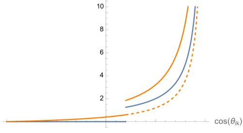
Figure 5: Blue: distribution of soft photon radiation from a dipole with opening angle $\cos\theta_{ij}=0.2$; Orange: corresponding result coming from the leading next-to-soft correction, as captured by the momentum shifts in eq. (32). The dashed line shows the non-angular ordered contribution to the next-to-soft result.

Here we have explicitly considered QED, where this pronounced radiation pattern is known as the Chudakov effect. The same arguments apply to QCD in the case of single gluon radiation from a dipole, where this is an overall colour singlet [14, 15]. In both cases, the simple quantum mechanical argument for the suppressed radiation outside the cone is that the wavelength of the emitted photon becomes such that it cannot resolve the individual (colour) charges in the dipole.

3.2 Next-to-soft radiation from a dipole

Having recalled how angular ordering arises from soft radiation, let us now examine how the additional momentum-shift corrections in eq. (32) modify the picture. To this end, we may again restrict ourselves to the simplest possible case of a final-state dipole in gauge theory, namely the electron-positron pair of figure 4(a). Then the effect of an additional photon emission up to next-to-soft level is to modify eq. (34) to

$$|{\cal M}_{\rm NLP}|^{2}\sim W_{ij}|{\cal M}^{(0)}(p_{i}-\delta p_{i,j},p_{j}-\delta p_{j,i})|^{2},$$ (47)

using the momentum shift definitions of eq. (27). Up to NLP level, we can expand to first order in the momentum shifts, and also use the fact that the squared Born interaction depends only on the Mandelstam invariant $s=2p_{i}\cdot p_{j}$, to get

$$|{\cal M}_{\rm NLP}|^{2}\sim W_{ij}f(s)-2\Big{[}\delta p_{i,j}\cdot p_{j}+\delta p_{j,i}\cdot p_{i}\Big{]}W_{ij}f^{\prime}(s),$$ (48)

where

$$f(s)=|{\cal M}^{(0)}|^{2}$$ (49)

is the squared Born amplitude with unshifted kinematics, and the prime denotes its first-order derivative. To examine the angular properties of the next-to-soft term, we define the dimensionless radiation functions

$$\widetilde{W}^{[l]}_{ij} =-\left(\frac{\delta p_{i,j}\cdot p_{j}}{E_{k}E_{j}}+\frac{\delta p_{j,i}\cdot p_{i}}{E_{k}E_{i}}\right)W^{[l]}_{ij},$$ (50)

such that

$$\widetilde{W}_{ij}=\widetilde{W}^{[i]}_{ij}+\widetilde{W}^{[j]}_{ij}=-\left(\frac{\delta p_{i,j}\cdot p_{j}}{E_{k}E_{j}}+\frac{\delta p_{j,i}\cdot p_{i}}{E_{k}E_{i}}\right)W^{[l]}_{ij}$$ (51)

controls the total next-to-soft correction to the radiation pattern. Using the parametrisation of eq. (38), we have

$$\widetilde{W}^{[i]}_{ij}=(1-\cos\theta_{ik})W_{ij}^{[i]}+(1-\cos\theta_{jk})W_{ij}^{[i]}.$$ (52)

In the first term, the prefactor is independent of the azimuthal angle $\phi_{iq}$, and thus does not affect the integration over the latter. We can thus reuse the previous result for the azimuthal integration of $W_{ij}^{[i]}$ when calculating the radiation pattern. In the second term of eq. (52), the prefactor cancels the singularity in $\cos\theta_{jk}$, such that one finds

$$\int_{0}^{2\pi}\frac{d\phi_{ik}}{2\pi}\widetilde{W}^{[i]}_{ij} =\frac{1}{2}\left[1+\frac{\cos\theta_{ik}-\cos\theta_{ij}}{|\cos\theta_{ik}-\cos\theta_{ij}|}\right]$$

$$\quad+\frac{1}{2}\int_{0}^{2\pi}\frac{d\phi_{ik}}{2\pi}\left[\frac{1-\cos\theta_{ij}}{1-\cos\theta_{ik}}+\frac{a-b\cos\phi_{ik}}{1-\cos\theta_{ik}}-1\right]$$

$$=\frac{1}{2}\left[1+\frac{\cos\theta_{ik}-\cos\theta_{ij}}{|\cos\theta_{ik}-\cos\theta_{ij}|}\right]+\sin^{2}\left(\frac{\theta_{ij}}{2}\right)\cot^{2}\left(\frac{\theta_{ik}}{2}\right).$$ (53)

This is our final result for the azimuthally-averaged next-to-soft radiation pattern from one particle in a dipole. Interestingly, it has the form of a sum of an angular-ordered term, analogous to the pure soft case, plus a breaking term, which has a remarkably compact analytic form. We show this function in figure 5, and can see clearly the effect of the angular-ordering term, in that there is a discontinuity at $\cos\theta_{ik}=\cos\theta_{ij}$. However, for $\cos\theta_{ik}<\cos\theta_{ij}$, corresponding to gluon emission outside the cone region, there is indeed a non-zero radiation distribution. For completeness, we show the effect of the non-angular-ordered term (i.e. the second term in eq. (53)) inside the cone. This is shown as the dashed line in figure 5, and we see that it smoothly joins the radiation outside the cone, as it should. There remains a (hard) collinear singularity around particle $i$, which acts as a next-to-soft correction to a collinear emission which is also strictly soft. In interpreting the figure, we must remember that the LP and NLP radiation functions ($W^{[i]}_{ij}$ and $\tilde{W}^{[i]}_{ij}$ respectively) are defined with different energy ratios to make them dimensionless. Thus, the overall normalisation between the two curves in figure 5 is not particularly meaningful. Rather, figure 5 illustrates the significant qualitative difference between the angular distributions of soft and next-to-soft radiation: the latter breaks angular ordering.

Note that a similar effect appears for massive emitters at leading soft level, as is well-known [14, 15]. Denoting the energy-normalised velocity of the two dipole legs with $v_{i}$ and $v_{j}$ respectively, one obtains for the azimuthally-averaged emission pattern

$$\int^{2\pi}_{0}\frac{d\phi_{ik}}{2\pi}W_{ij}^{[i]}=\frac{v_{i}}{2(1-v_{i}\cos\theta_{ik})}\left[\frac{v_{i}-\cos\theta_{ik}}{1-v_{i}\cos\theta_{ik}}+\frac{\cos\theta_{ik}-v_{j}\cos\theta_{ij}}{\sqrt{(\cos\theta_{ik}-v_{j}\cos\theta_{ij})^{2}+\sin\theta_{ik}^{2}(1-v_{j}^{2})}}\right].$$ (54)

This reduces to the massless form when $v_{i}=v_{j}=1$. However, when $v_{j}\neq 1$ (but $v_{i}=1$) the sharp transition is replaced by a smooth damping of the total radiation from the dipole, which extends to angles larger than the opening angle of the dipole. This is shown in figure 6, which contrasts the massless and massive cases. Here, the presence of an intrinsic momentum scale results in the breaking of angular-ordering, and it would be interesting to further examine the interplay between next-to-soft and massive effects.

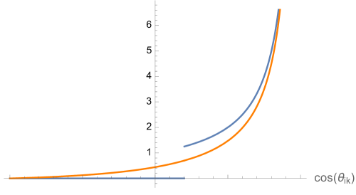
Figure 6: Blue: distribution of soft photon radiation from a dipole of massless particles with opening angle $\cos\theta_{ij}=0.2$; Orange: corresponding result if particle $j$ is massive, such that $v_{j}=0.5$ in eq. (54).

Let us now understand the next-to-soft effect in more physical terms. We can do this given that radiation outside the cone is associated with the specific momentum shifts in eq. (27), whose origin is the orbital angular momentum contributions to the squared matrix element. One can only generate such an orbital angular momentum if the two worldlines of the fermions in the dipole are mutually displaced. In particular, let us choose the origin of spacetime such that both lines are displaced to 4-positions $x^{\mu}_{i}$ and $x^{\mu}_{j}$, as shown in figure 4(b). The relationship between such displacements and next-to-soft corrections was considered in ref. [21], which used Schwinger proper time methods to write the scattering amplitude for hard particles emitting radiation in terms of quantum mechanical (first-quantised) path integrals over their spacetime trajectories. More specifically, one can show that such an amplitude is given by

$${\cal A}(p_{1},\ldots,p_{n})=\int{\cal D}A_{\mu}\left[\prod_{i=1}^{n}\int d^{d}x_{i}e^{-ip_{i}\cdot x_{i}}f(x_{i},p_{i};A_{\mu})\right]H(x_{1}\ldots x_{n};A_{\mu})e^{iS[A_{\mu}]},$$ (55)

where $H(x_{1},\ldots x_{n};A_{\mu})$ is a hard function that produces the outgoing particles at initial positions $\{x_{i}\}$ with final momenta $\{p_{i}\}$. The formal definition of this quantity can be found in ref. [21], and will not be needed in what follows. The path integral in eq. (55) is over the (next-to) soft gauge field, and includes the usual dependence on the action $S[A_{\mu}]$, where we suppress the dependence on the matter fields for brevity. Associated with each hard particle is an integral over its initial position $x_{i}$, a certain exponential factor, and further factor $f(x_{i},p_{i};A_{\mu})$, which for scalar particles is

$$f(x_{i},p_{i};A_{\mu})=\int{\cal D}z_{i}\exp\left[i\int_{0}^{\infty}d\tau\left(\frac{\dot{z}_{i}^{2}}{2}+q_{i}(\beta+\dot{x})\cdot A(x_{i}+\beta_{i}\tau+z_{i})+\frac{iq_{i}}{2}\partial\cdot A(x_{i}+\beta_{i}\tau+z_{i})\right)\right].$$ (56)

In this equation, we have parametrised the spacetime trajectory of the $i^{\rm th}$ particle via

$$x^{(i)}(t)=x_{i}+\beta_{i}\tau+z_{i}(\tau),$$ (57)

where $\beta_{i}$ is the 4-velocity associated with the final momentum $p_{i}$, and $\tau$ the proper time. The quantity $z_{i}(\tau)$ then constitutes a fluctuation about the classical straight-line trajectory, and the path integral over $z_{i}(\tau)$ corresponds to summing over all possible fluctuations. This path integral is carried out subject to the boundary conditions of fixed initial position $x_{i}$ and final momentum $p_{i}$ for each particle. Finally, $q_{i}$ is the electric charge of hard particle $i$.

As shown in ref. [21], the path integral over worldline trajectories in eq. (57) can be carried out perturbatively. The leading term – corresponding to keeping the classical trajectory only – amounts to the hard particle not recoiling, and thus emitting pure soft radiation only. Expanding order-by-order in $z_{i}(\tau)$ then amounts to including all possible wobbles in the spacetime trajectory which, by the uncertainty principle, amounts to including the emission of radiation at progressively subleading orders in the momentum of the emitted radiation. By keeping the first-order term only, ref. [21] found a set of Feynman rules corresponding to the emission of next-to-soft radiation from hard particles. Repeating the analysis for fermionic emitting particles leads to an extra term in eq. (56), that corresponds to the spin-dependent part of the next-to-soft theorem of eqs. (15, 16).

Now let us focus on the contribution to eq. (55) that stems from the initial separation of the dipole members, namely the non-zero initial positions $\{x_{i}\}$. At next-to-soft level, keeping track of these non-zero positions means that the path integral in eq. (56) can be replaced by its leading term (i.e. the classical trajectory only). The hard particle factor of eq. (56) then reduces to the well-known Wilson line describing the emission of soft radiation [21]:

$$f(x_{i},p_{i};A_{\mu}) \rightarrow\exp\left[iq_{i}\int_{0}^{\infty}d\tau\beta_{i}^{\mu}A_{\mu}(x_{i}+\beta_{i}\tau)\right]$$

$$=1-q_{i}\int\frac{d^{d}k}{(2\pi)^{d}}\frac{p_{i}^{\mu}\tilde{A}_{\mu}(k)}{p_{i}\cdot k}e^{ip_{i}\cdot k}+{\cal O}(q_{i}^{2}),$$ (58)

where we have transformed to momentum space in the second line, and expanded in the coupling so as to isolate the effect of a single photon emission in the second term. Next, we can expand the exponential appearing in the $k$ integral, where the first subleading correction corresponds to the next-to-soft contribution. Collecting these factors on all lines, the effect of the non-zero initial positions in the path integral of eq. (55) is

$$\left[\prod_{i=1}^{n}\int d^{d}x_{i}e^{-ix_{i}\cdot p_{i}}\right]\left[\sum_{j=1}^{n}q_{j}\frac{d^{d}k}{(2\pi)^{d}}(-ix_{j}\cdot k)\frac{p_{j}\cdot A(k)}{p_{j}\cdot k}\right]H(p_{1},\ldots,p_{n})=\Gamma^{\mu}A_{\mu},$$ (59)

where carrying out the integrals over the positions $\{x_{i}\}$ yields

$$\Gamma^{\mu}=\int\frac{d^{d}k}{(2\pi)^{d}}\sum_{j=1}^{n}q_{j}\left(\frac{p_{j}^{\mu}}{p_{j}\cdot k}k_{\nu}\frac{\partial}{\partial p_{j\nu}}\right)H(p_{1},\ldots,p_{n}).$$ (60)

In the path integral over the gauge field, this looks like an additional Feynman rule for the emission of a single photon from each line, which involves a derivative acting on the hard function. In fact, the result of eq. (59) is incomplete. In eq. (55), the hard function depends upon the gauge field, as it must. Expanding this order-by-order in the coupling amounts to including the effects of soft gluon emissions from inside the hard interaction (see ref. [21] for a detailed explanation). As shown in the very early work of ref. [70], such contributions can be fixed by gauge invariance. The most straightforward way to implement this here is to note that the factor $\Gamma^{\mu}$ will form part of a complete scattering amplitude ${\cal A}^{\mu}$ for the emission of a photon of momentum $k$, which must satisfy the Ward identity $k_{\mu}{\cal A}^{\mu}=0$. This in turn implies that we must modify

$$\Gamma^{\mu}\rightarrow\tilde{\Gamma}^{\mu},\quad k_{\mu}\tilde{\Gamma}^{\mu}=0.$$ (61)

Requiring a local combination of momenta yields the unique result (see also ref. [95])

$$\tilde{\Gamma}^{\mu}=\int\frac{d^{d}k}{(2\pi)^{d}}\sum_{j=1}^{n}q_{j}k_{\nu}\left(\frac{p_{j}^{\mu}}{p_{j}\cdot k}\frac{\partial}{\partial p_{j\nu}}-\frac{p_{j}^{\nu}}{p_{j}\cdot k}\frac{\partial}{\partial p_{j\mu}}\right)H(p_{1},\ldots,p_{n}).$$ (62)

Comparison with eq. (24) allows to explicitly recognise the form of the orbital angular momentum of each hard particle, a fact which was not clarified in ref. [21]. However, it makes precise the above expectation, that non-zero initial positions of the dipole members will indeed give rise to the orbital angular momentum part of the next-to-soft theorem.

The physics of angular-ordering breaking is then as follows. Soft radiation has an infinite Compton wavelength, and thus is unable to see the separation between the two fermion worldlines, as they emanate from a given hard interaction. Next-to-soft radiation, on the other hand, is able to resolve the length scale corresponding to the difference in initial particle positions, which manifests itself in the orbital angular momentum contributions being non-zero, as captured by the momentum shifts in eq. (32). The fact that wide-angle radiation now sees the initial “size” of the dipole means that it will no longer see a zero net charge. Hence, radiation can be present outside the cone.

4 Conclusion

In this paper, we have performed a case study looking at the physical interpretation of next-to-soft radiation. The characterisation of such radiation is of great interest in furthering the precision frontier at current collider experiments, as well as addressing interesting conceptual questions in field theory. In addition to building up new methods and techniques, it is important to build intuition about next-to-soft physics, that may in turn inform further developments. With this motivation in mind, we have here focused on a particular formula for incorporating gluon radiation using a dipole-like formula that incorporates next-to-soft effects through shifts of the momenta appearing in the non-radiative amplitude. This formula first appeared for colour-singlet final states in ref. [31], and was extended to particular processes with partons in the final state in ref. [32]. We have here checked its validity in another process ($Wg$ production). Next, we looked at the physical consequences of this formula, which stem from the fact that it has the form of a sum of dipole-like contributions.

One of the most well-known properties of soft emission from dipoles is that interference effects lead to suppression of the radiation outside cones surrounding each hard particle, whose half-angle corresponds to the opening angle between the constituents of the dipole. Faced with eq. (32), then, we can ask if the inclusion of next-to-soft corrections breaks the angular-ordering property. Indeed it does, and the physical mechanism of this is that the momentum shifts capture precisely that part of the next-to-soft physics – orbital angular momentum contributions – that is associated with an initial separation between the dipole constituents. This provides a new length scale, which the radiation is then able to resolve. Although this creates some radiation outside the cones described above, there still remains a significant discontinuity in the radiation distribution at the edge of the cone.

We hope that our results provide useful physical intuition to researchers working in this area, as well as inspiring further similar studies.

References

- [1] G. Parisi, Summing Large Perturbative Corrections in QCD, Phys. Lett. B 90 (1980) 295–296.
- [2] G. Curci and M. Greco, Large Infrared Corrections in QCD Processes, Phys. Lett. B92 (1980) 175–178.
- [3] G. Sterman, Summation of large corrections to short distance hadronic cross-sections, Nucl. Phys. B281 (1987) 310.
- [4] S. Catani and L. Trentadue, Resummation of the QCD Perturbative Series for Hard Processes, Nucl. Phys. B327 (1989) 323.
- [5] J. G. M. Gatheral, Exponentiation of eikonal cross-sections in nonabelian gauge theories, Phys. Lett. B133 (1983) 90.
- [6] J. Frenkel and J. C. Taylor, Nonabelian eikonal exponentiation, Nucl. Phys. B246 (1984) 231.
- [7] G. Sterman, Infrared divergences in perturbative QCD, . in Tallahassee 1981, Proceedings, Perturbative Quantum Chromodynamics, 22-40.
- [8] G. P. Korchemsky and G. Marchesini, Structure function for large x and renormalization of Wilson loop, Nucl. Phys. B 406 (1993) 225–258, [hep-ph/9210281].
- [9] G. P. Korchemsky and G. Marchesini, Resummation of large infrared corrections using Wilson loops, Phys. Lett. B313 (1993) 433–440.
- [10] T. Becher and M. Neubert, Threshold resummation in momentum space from effective field theory, Phys. Rev. Lett. 97 (2006) 082001, [hep-ph/0605050].
- [11] M. D. Schwartz, Resummation and NLO matching of event shapes with effective field theory, Phys.Rev. D77 (2008) 014026, [arXiv:0709.2709].
- [12] C. W. Bauer, S. P. Fleming, C. Lee, and G. F. Sterman, Factorization of e+e- Event Shape Distributions with Hadronic Final States in Soft Collinear Effective Theory, Phys.Rev. D78 (2008) 034027, [arXiv:0801.4569].
- [13] J.-y. Chiu, A. Fuhrer, R. Kelley, and A. V. Manohar, Factorization Structure of Gauge Theory Amplitudes and Application to Hard Scattering Processes at the LHC, Phys.Rev. D80 (2009) 094013, [arXiv:0909.0012].
- [14] R. K. Ellis, W. J. Stirling, and B. R. Webber, QCD and collider physics, Camb. Monogr. Part. Phys. Nucl. Phys. Cosmol. 8 (1996) 1–435.
- [15] J. Campbell, J. Huston, and F. Krauss, The Black Book of Quantum Chromodynamics. Oxford University Press, 2017.
- [16] G. Grunberg and V. Ravindran, On threshold resummation beyond leading 1-x order, JHEP 10 (2009) 055, [arXiv:0902.2702].
- [17] G. Soar, S. Moch, J. Vermaseren, and A. Vogt, On Higgs-exchange DIS, physical evolution kernels and fourth-order splitting functions at large x, Nucl.Phys. B832 (2010) 152–227, [arXiv:0912.0369].
- [18] S. Moch and A. Vogt, On non-singlet physical evolution kernels and large-x coefficient functions in perturbative QCD, JHEP 11 (2009) 099, [arXiv:0909.2124].
- [19] S. Moch and A. Vogt, Threshold Resummation of the Structure Function F(L), JHEP 04 (2009) 081, [arXiv:0902.2342].
- [20] E. Laenen, L. Magnea, G. Stavenga, and C. D. White, Next-to-eikonal corrections to soft gluon radiation: a diagrammatic approach, JHEP 1101 (2011) 141, [arXiv:1010.1860].
- [21] E. Laenen, G. Stavenga, and C. D. White, Path integral approach to eikonal and next-to-eikonal exponentiation, JHEP 03 (2009) 054, [arXiv:0811.2067].
- [22] D. de Florian, J. Mazzitelli, S. Moch, and A. Vogt, Approximate N3LO Higgs-boson production cross section using physical-kernel constraints, JHEP 10 (2014) 176, [arXiv:1408.6277].
- [23] N. Lo Presti, A. Almasy, and A. Vogt, Leading large-x logarithms of the quark & gluon contributions to inclusive Higgs-boson and lepton-pair production, Phys. Lett. B737 (2014) 120–123, [arXiv:1407.1553].
- [24] D. Bonocore, E. Laenen, L. Magnea, S. Melville, L. Vernazza, and C. D. White, A factorization approach to next-to-leading-power threshold logarithms, JHEP 06 (2015) 008, [arXiv:1503.05156].
- [25] D. Bonocore, E. Laenen, L. Magnea, L. Vernazza, and C. D. White, Non-abelian factorisation for next-to-leading-power threshold logarithms, JHEP 12 (2016) 121, [arXiv:1610.06842].
- [26] D. Bonocore, Asymptotic dynamics on the worldline for spinning particles, JHEP 02 (2021) 007, [arXiv:2009.07863].
- [27] H. Gervais, Soft Photon Theorem for High Energy Amplitudes in Yukawa and Scalar Theories, Phys. Rev. D95 (2017), no. 12 125009, [arXiv:1704.00806].
- [28] H. Gervais, Soft Graviton Emission at High and Low Energies in Yukawa and Scalar Theories, Phys. Rev. D96 (2017), no. 6 065007, [arXiv:1706.03453].
- [29] H. Gervais, Soft Radiation Theorems at All Loop Order in Quantum Field Theory. PhD thesis, SUNY, Stony Brook, 2017-08-04.
- [30] E. Laenen, J. Sinninghe Damsté, L. Vernazza, W. Waalewijn, and L. Zoppi, Towards all-order factorization of QED amplitudes at next-to-leading power, Phys. Rev. D103 (2021), no. 3 034022, [arXiv:2008.01736].
- [31] V. Del Duca, E. Laenen, L. Magnea, L. Vernazza, and C. D. White, Universality of next-to-leading power threshold effects for colourless final states in hadronic collisions, JHEP 11 (2017) 057, [arXiv:1706.04018].
- [32] M. van Beekveld, W. Beenakker, E. Laenen, and C. D. White, Next-to-leading power threshold effects for inclusive and exclusive processes with final state jets, JHEP 03 (2020) 106, [arXiv:1905.08741].
- [33] D. Bonocore, E. Laenen, L. Magnea, L. Vernazza, and C. D. White, The method of regions and next-to-soft corrections in Drell-Yan production, Phys. Lett. B742 (2015) 375–382, [arXiv:1410.6406].
- [34] N. Bahjat-Abbas, J. Sinninghe Damsté, L. Vernazza, and C. D. White, On next-to-leading power threshold corrections in Drell-Yan production at N3LO, JHEP 10 (2018) 144, [arXiv:1807.09246].
- [35] M. A. Ebert, I. Moult, I. W. Stewart, F. J. Tackmann, G. Vita, and H. X. Zhu, Power Corrections for N-Jettiness Subtractions at , JHEP 12 (2018) 084, [arXiv:1807.10764].
- [36] R. Boughezal, A. Isgrò, and F. Petriello, Next-to-leading-logarithmic power corrections for -jettiness subtraction in color-singlet production, Phys. Rev. D97 (2018), no. 7 076006, [arXiv:1802.00456].
- [37] R. Boughezal, A. Isgrò, and F. Petriello, Next-to-leading power corrections to jet production in -jettiness subtraction, Phys. Rev. D101 (2020), no. 1 016005, [arXiv:1907.12213].
- [38] N. Bahjat-Abbas, D. Bonocore, J. Sinninghe Damsté, E. Laenen, L. Magnea, L. Vernazza, and C. D. White, Diagrammatic resummation of leading-logarithmic threshold effects at next-to-leading power, JHEP 11 (2019) 002, [arXiv:1905.13710].
- [39] A. H. Ajjath, P. Mukherjee, and V. Ravindran, On next to soft corrections to Drell-Yan and Higgs Boson productions, arXiv:2006.06726.
- [40] A. H. Ajjath, P. Mukherjee, V. Ravindran, A. Sankar, and S. Tiwari, On next to soft threshold corrections to DIS and SIA processes, JHEP 04 (2021) 131, [arXiv:2007.12214].
- [41] A. H. Ajjath, P. Mukherjee, V. Ravindran, A. Sankar, and S. Tiwari, On next to soft corrections for Drell-Yan and Higgs boson rapidity distributions beyond N3LO, Phys. Rev. D103 (2021) L111502, [arXiv:2010.00079].
- [42] T. Ahmed, A. A. H., P. Mukherjee, V. Ravindran, and A. Sankar, Soft-virtual correction and threshold resummation for -colorless particles to fourth order in QCD: Part II, arXiv:2010.02980.
- [43] T. Ahmed, A. H. Ajjath, G. Das, P. Mukherjee, V. Ravindran, and S. Tiwari, Soft-virtual correction and threshold resummation for -colorless particles to fourth order in QCD: Part I, arXiv:2010.02979.
- [44] A. H. Ajjath, P. Mukherjee, V. Ravindran, A. Sankar, and S. Tiwari, Next-to SV resummed Drell-Yan cross section beyond leading-logarithm, arXiv:2107.09717.
- [45] D. W. Kolodrubetz, I. Moult, and I. W. Stewart, Building Blocks for Subleading Helicity Operators, JHEP 05 (2016) 139, [arXiv:1601.02607].
- [46] I. Moult, L. Rothen, I. W. Stewart, F. J. Tackmann, and H. X. Zhu, Subleading Power Corrections for N-Jettiness Subtractions, Phys. Rev. D95 (2017), no. 7 074023, [arXiv:1612.00450].
- [47] I. Feige, D. W. Kolodrubetz, I. Moult, and I. W. Stewart, A Complete Basis of Helicity Operators for Subleading Factorization, JHEP 11 (2017) 142, [arXiv:1703.03411].
- [48] M. Beneke, M. Garny, R. Szafron, and J. Wang, Anomalous dimension of subleading-power N-jet operators, JHEP 03 (2018) 001, [arXiv:1712.04416].
- [49] M. Beneke, M. Garny, R. Szafron, and J. Wang, Anomalous dimension of subleading-power -jet operators. Part II, JHEP 11 (2018) 112, [arXiv:1808.04742].
- [50] A. Bhattacharya, I. Moult, I. W. Stewart, and G. Vita, Helicity Methods for High Multiplicity Subleading Soft and Collinear Limits, JHEP 05 (2019) 192, [arXiv:1812.06950].
- [51] M. Beneke, M. Garny, R. Szafron, and J. Wang, Violation of the Kluberg-Stern-Zuber theorem in SCET, JHEP 09 (2019) 101, [arXiv:1907.05463].
- [52] G. T. Bodwin, J.-H. Ee, J. Lee, and X.-P. Wang, Renormalization of the radiative jet function, arXiv:2107.07941.
- [53] I. Moult, I. W. Stewart, and G. Vita, Subleading Power Factorization with Radiative Functions, JHEP 11 (2019) 153, [arXiv:1905.07411].
- [54] M. Beneke, A. Broggio, S. Jaskiewicz, and L. Vernazza, Threshold factorization of the Drell-Yan process at next-to-leading power, JHEP 07 (2020) 078, [arXiv:1912.01585].
- [55] Z. L. Liu and M. Neubert, Factorization at subleading power and endpoint-divergent convolutions in decay, JHEP 04 (2020) 033, [arXiv:1912.08818].
- [56] Z. L. Liu, B. Mecaj, M. Neubert, and X. Wang, Factorization at subleading power, Sudakov resummation, and endpoint divergences in soft-collinear effective theory, Phys. Rev. D104 (2021), no. 1 014004, [arXiv:2009.04456].
- [57] R. Boughezal, X. Liu, and F. Petriello, Power Corrections in the N-jettiness Subtraction Scheme, JHEP 03 (2017) 160, [arXiv:1612.02911].
- [58] I. Moult, I. W. Stewart, and G. Vita, A subleading operator basis and matching for gg → H, JHEP 07 (2017) 067, [arXiv:1703.03408].
- [59] C.-H. Chang, I. W. Stewart, and G. Vita, A Subleading Power Operator Basis for the Scalar Quark Current, JHEP 04 (2018) 041, [arXiv:1712.04343].
- [60] I. Moult, I. W. Stewart, G. Vita, and H. X. Zhu, First Subleading Power Resummation for Event Shapes, JHEP 08 (2018) 013, [arXiv:1804.04665].
- [61] M. Beneke, A. Broggio, M. Garny, S. Jaskiewicz, R. Szafron, L. Vernazza, and J. Wang, Leading-logarithmic threshold resummation of the Drell-Yan process at next-to-leading power, JHEP 03 (2019) 043, [arXiv:1809.10631].
- [62] M. A. Ebert, I. Moult, I. W. Stewart, F. J. Tackmann, G. Vita, and H. X. Zhu, Subleading power rapidity divergences and power corrections for qT, JHEP 04 (2019) 123, [arXiv:1812.08189].
- [63] M. Beneke, M. Garny, S. Jaskiewicz, R. Szafron, L. Vernazza, and J. Wang, Leading-logarithmic threshold resummation of Higgs production in gluon fusion at next-to-leading power, JHEP 01 (2020) 094, [arXiv:1910.12685].
- [64] I. Moult, I. W. Stewart, G. Vita, and H. X. Zhu, The Soft Quark Sudakov, JHEP 05 (2020) 089, [arXiv:1910.14038].
- [65] Z. L. Liu and M. Neubert, Two-Loop Radiative Jet Function for Exclusive -Meson and Higgs Decays, JHEP 06 (2020) 060, [arXiv:2003.03393].
- [66] Z. L. Liu, B. Mecaj, M. Neubert, X. Wang, and S. Fleming, Renormalization and Scale Evolution of the Soft-Quark Soft Function, JHEP 07 (2020) 104, [arXiv:2005.03013].
- [67] J. Wang, Resummation of double logarithms in loop-induced processes with effective field theory, arXiv:1912.09920.
- [68] M. Beneke, M. Garny, S. Jaskiewicz, R. Szafron, L. Vernazza, and J. Wang, Large-x resummation of off-diagonal deep-inelastic parton scattering from d-dimensional refactorization, JHEP 10 (2020) 196, [arXiv:2008.04943].
- [69] M. van Beekveld, L. Vernazza, and C. D. White, Threshold resummation of new partonic channels at next-to-leading power, JHEP 12 (2021) 087, [arXiv:2109.09752].
- [70] F. E. Low, Bremsstrahlung of very low-energy quanta in elementary particle collisions, Phys. Rev. 110 (1958) 974–977.
- [71] T. H. Burnett and N. M. Kroll, Extension of the low soft photon theorem, Phys. Rev. Lett. 20 (1968) 86.
- [72] V. Del Duca, High-energy bremsstrahlung theorems for soft photons, Nucl. Phys. B345 (1990) 369–388.
- [73] M. Kramer, E. Laenen, and M. Spira, Soft gluon radiation in Higgs boson production at the LHC, Nucl. Phys. B511 (1998) 523–549, [hep-ph/9611272].
- [74] R. D. Ball, M. Bonvini, S. Forte, S. Marzani, and G. Ridolfi, Higgs production in gluon fusion beyond NNLO, Nucl.Phys. B874 (2013) 746–772, [arXiv:1303.3590].
- [75] M. Bonvini, S. Forte, G. Ridolfi, and L. Rottoli, Resummation prescriptions and ambiguities in SCET vs. direct QCD: Higgs production as a case study, JHEP 01 (2015) 046, [arXiv:1409.0864].
- [76] C. Anastasiou, C. Duhr, F. Dulat, F. Herzog, and B. Mistlberger, Higgs Boson Gluon-Fusion Production in QCD at Three Loops, Phys. Rev. Lett. 114 (2015) 212001, [arXiv:1503.06056].
- [77] C. Anastasiou, C. Duhr, F. Dulat, E. Furlan, T. Gehrmann, F. Herzog, A. Lazopoulos, and B. Mistlberger, High precision determination of the gluon fusion Higgs boson cross-section at the LHC, JHEP 05 (2016) 058, [arXiv:1602.00695].
- [78] M. van Beekveld, W. Beenakker, R. Basu, E. Laenen, A. Misra, and P. Motylinski, Next-to-leading power threshold effects for resummed prompt photon production, Phys. Rev. D100 (2019), no. 5 056009, [arXiv:1905.11771].
- [79] M. van Beekveld, E. Laenen, J. Sinninghe Damsté, and L. Vernazza, Next-to-leading power threshold corrections for finite order and resummed colour-singlet cross sections, JHEP 05 (2021) 114, [arXiv:2101.07270].
- [80] G. Sterman and W. Vogelsang, Power corrections to electroweak boson production from threshold resummation, Phys. Rev. D 107 (2023), no. 1 014009, [arXiv:2208.00937].
- [81] M. Czakon, F. Eschment, and T. Schellenberger, Subleading Effects in Soft-Gluon Emission at One-Loop in Massless QCD, arXiv:2307.02286.
- [82] J. Smith, D. Thomas, and W. L. van Neerven, QCD Corrections to the Reaction X, Z. Phys. C 44 (1989) 267.
- [83] W. T. Giele, E. W. N. Glover, and D. A. Kosower, Higher order corrections to jet cross-sections in hadron colliders, Nucl. Phys. B403 (1993) 633–670, [hep-ph/9302225].
- [84] J. A. M. Vermaseren, New features of form, math-ph/0010025.
- [85] J. Kublbeck, H. Eck, and R. Mertig, Computeralgebraic generation and calculation of Feynman graphs using FeynArts and FeynCalc, Nucl.Phys.Proc.Suppl. 29A (1992) 204–208.
- [86] S. Frixione, A next-to-leading order calculation of the cross-section for the production of w+ w- pairs in hadronic collisions, Nucl. Phys. B410 (1993) 280–324.
- [87] S. Catani and M. H. Seymour, A general algorithm for calculating jet cross-sections in nlo qcd, Nucl. Phys. B485 (1997) 291–419, [hep-ph/9605323].
- [88] S. Catani and M. H. Seymour, The dipole formalism for the calculation of qcd jet cross- sections at next-to-leading order, Phys. Lett. B378 (1996) 287–301, [hep-ph/9602277].
- [89] F. Cachazo and A. Strominger, Evidence for a New Soft Graviton Theorem, arXiv:1404.4091.
- [90] E. Casali, Soft sub-leading divergences in Yang-Mills amplitudes, JHEP 08 (2014) 077, [arXiv:1404.5551].
- [91] C. White, Diagrammatic insights into next-to-soft corrections, Phys. Lett. B737 (2014) 216–222, [arXiv:1406.7184].
- [92] C. D. White, The SAGEX Review on Scattering Amplitudes, Chapter 12: Amplitudes and collider physics, arXiv:2203.13023.
- [93] S. Pasterski, S.-H. Shao, and A. Strominger, Flat Space Amplitudes and Conformal Symmetry of the Celestial Sphere, Phys. Rev. D 96 (2017), no. 6 065026, [arXiv:1701.00049].
- [94] S. Pasterski and S.-H. Shao, Conformal basis for flat space amplitudes, Phys. Rev. D 96 (2017), no. 6 065022, [arXiv:1705.01027].
- [95] Z. Bern, S. Davies, and J. Nohle, On Loop Corrections to Subleading Soft Behavior of Gluons and Gravitons, Phys. Rev. D90 (2014), no. 8 085015, [arXiv:1405.1015].