Denoising Particle-In-Cell Data via Smoothness-Increasing Accuracy-Conserving Filters with Application to Bohm Speed Computation

Abstract

The simulation of plasma physics is computationally expensive because the underlying physical system is of high dimensions, requiring three spatial dimensions and three velocity dimensions. One popular numerical approach is Particle-In-Cell (PIC) methods owing to its ease of implementation and favorable scalability in high-dimensional problems. An unfortunate drawback of the method is the introduction of statistical noise resulting from the use of finitely many particles. In this paper we examine the application of the Smoothness-Increasing Accuracy-Conserving (SIAC) family of convolution kernel filters as denoisers for moment data arising from PIC simulations. We show that SIAC filtering is a promising tool to denoise PIC data in the physical space as well as capture the appropriate scales in the Fourier space. Furthermore, we demonstrate how the application of the SIAC technique reduces the amount of information necessary in the computation of quantities of interest in plasma physics such as the Bohm speed.

1 Introduction

With the high-dimensionality of the equations governing plasma kinetics in six dimensional phase space [1], traditional numerical techniques for solving partial differential equations (PDE) suffer from the curse of dimensionality. This motivated the development and application of Particle-In-Cell (PIC) methods that have been a staple in plasma kinetic simulations  [2, 3]. The particle-based approach provides simplicity and geometric flexibility, but these benefits come at the expense of siginificant amount of noise, which scales as $1/\sqrt{N}$ with $N$ the number of particle markers in a cell. As an example, for a resolution of $10^{4}$ particle markers per cell, the noise level is still about 1%. Remarkably, finite amounts of noise, even at substantial level, does not generally prevent a physics-wise meaningful PIC simulation. For example, demonstration of Laudau damping can be achieved with a rather modest $N$, except that the post-run physics analysis is hampered by the noisy diagnostics. The difficulty is aggravated by the fact that the underlying physics is usually described, in the standard statistical physics approach, by velocity moments of the particle distribution function $f(\mathbf{x},\mathbf{v},t)$,

$$\left<v_{i}^{k}\right>=\int v_{i}^{k}f(\mathbf{x},\mathbf{v},t)\;d^{3}\mathbf{v},$$ (1)

with $v_{i}$ the cartesian component of $\mathbf{v}.$ For example, the thermodynamic state variables have the density $n(\mathbf{x},t)\equiv\left<\mathbf{v}^{0}\right>,$ the flow $\mathbf{U}(\mathbf{x},t)\equiv\left<\mathbf{v}\right>/n,$ and the temperature $T(\mathbf{x},t)\equiv(m/2)\left(\left<|\mathbf{v}|^{2}\right>/n-|\mathbf{U}|^{2}\right).$ Closure quantities such as the plasma heat flux involve even higher order velocity moments, for example,

$$\mathbf{q}\equiv\frac{m}{2}\left<\left(\mathbf{v}-\mathbf{U}\right)^{3}\right>.$$ (2)

The general rule of thumb is that the particle noise becomes further exaggerated in higher order moment quantities. In Fig. 1, we show the fluctuations in commonly used physical quantities that are obtained by post-processing particle data from a PIC simulation. This high level of noise in the post-processed physical quantities hampers our ability to gain deep insights into the underlying physics.

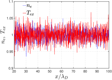
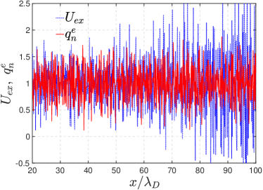
Figure 1: Electron density $n_{e}$ and temperature $T_{ex}$ (left figure), and the flow $U_{ex}$ and thermal conduction heat flux $q_{n}^{e}$ (right figure) from 1D3V PIC simulations of a plasma thermal quench with absorbing boundary from Ref. [4], where 5,000 particles per cell were used. All the variables are normalized by their denoised post-processed quantities.

A recent work on the Bohm criterion analysis [5] that establishes the lower bound of the plasma outflow speed, also known as the Bohm speed [6], in a wall-bounded plasma with finite collisionality, illustrates the extent one has to go to overcome the PIC noise in order to decipher the underlying physics. Specifically, the Bohm speed is predicted by theoretical analysis to take the form of

$$u_{Bohm}\equiv\sqrt{\frac{Z\beta T^{se}_{ex}+3T^{se}_{ix}}{m_{i}}},$$ (3)

where

$$\beta\equiv\frac{3-\frac{3+2\alpha}{Ze\Gamma^{se}_{i}}\Big{(}\frac{\partial q^{i}_{n}}{\partial\phi}+\frac{Q_{ii}}{E}\Big{)}+\frac{\alpha}{e\Gamma^{se}_{e}}\Big{(}\frac{\partial q^{e}_{n}}{\partial\phi}+\frac{Q_{ee}+Q_{ei}}{E}\Big{)}}{1+\frac{1+\alpha}{e\Gamma^{se}_{e}}\Big{(}\frac{\partial q^{e}_{n}}{\partial\phi}+\frac{Q_{ee}+Q_{ei}}{E}\Big{)}},$$ (4)

with $\Gamma_{e,i}=n_{e,i}u_{e,ix}$, $\partial q^{e,i}_{n}/\partial\phi=-(\partial q^{e,i}_{n}/\partial x)/E$, $\alpha=-R_{T}/(n_{e}\partial T_{ex}/\partial x)$ being the thermal force coefficient, $Z$ the ion charge state, $m_{i}$ the ion mass, and $e$ the elementary charge. The plasma transport physics are in the form of local electric field $E$, which is proportional to spatial gradient of the potential ($\phi$), particle and heat fluxes (which are denoted by $\Gamma_{e,i}$ and $q_{n}^{e,i}$, respectively), collisional energy exchange between electrons $(Q_{ee})$ and between electrons and ions $(Q_{ei})$, electron and ion temperatures $(T_{ex},T_{ix})$, respectively, and the thermal force ($R_{T}$). Here the superscript $se$ denotes the spatial location at which all quantities are to be evaluated to find the local Bohm speed, and the subscripts $e,i$ stands for the electron and ion quantities, respectively, and $x$ represents the x-component of the variable. Most of these quantities are simply velocity moments of the computed distribution function, or the velocity moments of the Coulomb collisional integral, and quantities that are derived from them. The PIC noise thus makes it an extremely difficult task to directly compare the numerical simulation results with theoretical predictions. Ref. [5] overcame this hurdle by performing long-time simulations after a steady-state is reached, and then applying time averaging over an extremely long-period of PIC data to control the PIC noise to be a sufficiently low level so that a definite comparison with Eqs. (3) and (4) can be done. This effectively increases $N$ from $10^{3-4}$ markers per cell to tens of millions per cell by accumulating data over time. Powerful and computationally expensive as this approach is, many applications do not even allow a steady-state solution. To decipher subtle transport physics from PIC simulations, one must therefore explore alternative approaches to effectively deal with PIC noise when modestly large $N$ and limited time-window averaging are available. We note that the regression and denoising approaches applied to the velocity space of PIC simulations are available, such as those based on Gaussian mixtures [7, 8]. Other denoising approaches for PIC code include the $\delta f$ approach [9, 10], sparse grid techniques [11, 12], phase space smoothing [13, 14], wavelet denoising [15], etc. Our work aims to propose and explore a distinctive approach tailored for PIC moments.

Here we address this issue through the use of Smoothness-Increasing Accuracy-Conserving (SIAC) filters which were originally developed as a post-processor for extracting superconvergence from finite element method (FEM) based numerical approximations [16]. The purpose of this paper is to demonstrate the effectiveness of SIAC filtering in “offline” noise reduction of pointwise data arising from PIC simulations. We will show that the application of specially tuned SIAC convolution kernels can selectively remove high frequency oscillations without polluting the intended low-frequency information, and thereby improve approximation quality. Extensions of the filtering procedure for non-periodic data are constructed, and results are shown for how SIAC filtering schemes can reduce the quantity of data needed in computing the Bohm speed, an important parameter in plasma physics bounding from below the ion velocity to a charged boundary. In these later examples, the spatial tuning requires the kernel scaling to be adjusted for both the variable being filtered as well as the location within the domain.

The rest of the paper is organized in as follows. In Sec. 2 we describe a procedure for initializing an approximation in a continuous variable from discrete data using Lagrange polynomials. In Sec. 3 we describe the construction of symmetric and position-dependent SIAC kernels which we convolve with our initialization dampen high-frequency oscillations. Boundary treatments as well as adaptive kernel scalings are also discussed. Lastly, in Sec. 4 we provide numerical examples detailing the damping effects of symmetric kernel on periodic data, adaptively scaled and position-dependent generalized spline kernels for non-periodic data, and data reduction enabled by SIAC filtering in Bohm speed computation.

(a)		(b)

Figure 2: Example of partitioning pointwise PIC data into elements, and constructing an interpolant of the pointwise data $(f_{j}=f(x_{j}))$ on each element. The red partitions represent the superimposed mesh to the pointwise grid. The blue lines represent the piecewise linear interpolant reconstructed from a stencil containing two grid values. In (a) the elements $\tau_{j}=I_{j}$ consist of a single cell, and the stencil uses information from the right adjacent cell ($\ell=0$ and $r=1$). In (b) the elements $\tau_{j}=I_{2j-1}\cup I_{2j}$ are formed of a union of two neighboring cells and the stencil for each element only consists of those cells inside that element.

2 Data Initialization

Unlike traditional FEM data which is defined over the entirety of a given mesh, the data considered here arises from moments of PIC simulations and is discrete in nature. SIAC filtering makes use of a continuous convolution, therefore to apply SIAC filtering a global representation must be constructed. The methodology presented here is to superimpose a mesh over the pointwise grid where the data is defined. For simplicity, within each element of this mesh, we construct a Lagrange interpolant from the pointwise data using a stencil of a chosen size. For ease of illustration we consider the one-dimensional case.

2.1 Constructing the mesh

Consider a domain $\Omega=[a,b]$, and assume that the pointwise data $\{f_{j}\}^{N}_{j=1}$ is given on the cell centers of a grid

$$a<x_{1}<x_{2}<\ldots<x_{N-1}<x_{N}<b.$$

Thinking about the data from a finite volume perspective, introduce cells $I_{j}=[x_{j-1/2},x_{j+1/2}]$, $j=1,\ldots,N$, where $x_{j-1/2}=\frac{1}{2}(x_{j}-x_{j-1})$, with $x_{1/2}=a$ and $x_{N+1/2}=b$. Denote the cell widths by $\Delta x_{j}=x_{j+1/2}-x_{j-1/2}$. It is possible to choose the elements of the superimposed mesh, ${\mathcal{T}=}\{\tau_{k}\}_{k=1}^{N_{\tau}}$, to just be these cells, in which case the mesh will be similar to that depicted in Fig. 2(a). Alternatively, the elements can be selected to be a union of adjacent cells, an example of which is given in Fig. 2(b). This choice will cause no difficulty in what follows, it only alters the number of polynomial interpolants needed in the construction, $N_{\tau}$, and the minimum stencil size of these interpolants. In the numerical implementation, only the cases of elements consisting of one or two cells is considered.

2.2 Constructing a piecewise polynomial interpolant

To convert the discrete data into a continuous approximation on a given element $\tau{{}_{k}}$, we choose nonnegative integers $\ell$ and $r$ and introduce the stencil about element $I_{j}:$

$$S(j)=\{I_{j-\ell},\ldots,I_{j},\ldots,I_{j+r}\}.$$

Assume here that the center cell of the stencil, $I_{j}$, satisfies $I_{j}\subset\tau{{}_{k}}$. The pointwise data contained within the cells of this stencil will be used to construct the interpolant over $\tau{{}_{k}}$. Note that the lack of assumptions about boundary conditions necessitates that the stencil is reduced in size near domain boundaries in order to not exceed the boundaries of our domain. Setting $p=\ell+r$, the Lagrange basis specific to the element is $\{L^{j}_{q}(x)\}_{q=0}^{p}$, with

$$L^{j}_{q}(x)=\prod_{\begin{subarray}{c}n=0\\ n\neq q\end{subarray}}^{p}\frac{x-x_{n+j-\ell}}{x_{q+j-\ell}-x_{n+j-\ell}}.$$

The element-specific interpolant is then given by

$$u_{h}(x)\Big{|}_{\tau}=\sum_{q=0}^{p}f_{q+j-\ell}L^{j}_{q}(x).$$

Iterating through the elements, and restricting the stencils where appropriate, a piecewise polynomial representation of the pointwise data over the whole domain is obtained. In the work to follow we find there is no significant difference in using larger stencils for the initialization procedure. To that end, here a finite-volume perspective is used and the discrete data is treated as cell-center values on a finite-volume style mesh. This corresponds to a $p=0$ piecewise-constant initialization.

3 SIAC Filters: Kernel Construction and Boundary Treatments

This section describes a convolution denoising procedure and the construction of the SIAC kernel used in the convolution. For ease of illustration we again consider the one-dimensional case.

The filtered data, $u^{\star}_{h}$, is obtained via convolution of the interpolant, $u_{h}$, with a compactly supported scaled kernel function $K_{H}$:

$$u^{\star}_{h}(x)=K_{H}\star u_{h}\equiv\int_{\mathbb{R}}K_{H}(x-y)\,u_{h}(y)\;dy.$$ (5)

Here, a family of kernel functions known as SIAC kernels is considered. These SIAC kernels are piecewise polynomial functions of compact support that satisfy consistency and moment conditions, which will be discussed in Sec. 3.4. It is important to note that the compact support of the kernel function reduces the integral in Eq. (5) from the entire range of $\mathbb{R}$ to a shifted support of the kernel. In applying the filter to non-periodic data, it is exactly this restriction of the kernel’s support that enables shifted or position-dependent kernels to constrict the convolution to within the domain of the data. In the following, a review of several types of SIAC kernels for applications to both periodic and non-periodic data is given. In the latter case, a description of the position-dependent kernels developed in [17] and the generalized spline boundary kernels introduced in [18] is given, as well as an introduction to a novel adaptive kernel scaling based on [19].

3.1 Kernel formulation

The knot matrix formulation of the SIAC kernel introduced in [18] is used. This description encompasses both the symmetric formulation for periodic data and the position-dependent formulation for non-periodic data. The SIAC kernel composed of $(r+1)$ B-splines of order $\ell$ is defined via an $(r+1)\times(\ell)$ knot matrix $\mathbf{T}$ which will be given in Sec. 3.3. The composite kernel is given by

$$K_{\mathbf{T}}(x)=\sum_{\gamma=0}^{r}c_{\gamma}B^{\ell}_{\mathbf{T}_{\gamma}}(x),$$

where $\mathbf{T}_{\gamma}=\mathbf{T}(\gamma,:)$ denotes the $\gamma$-th row of $\mathbf{T}$ for $\gamma=0,1,\ldots,r$. These rows contain the knot sequences for each B-spline composing the kernel. As detailed in [20] the $j$-th B-spline of order $\ell$ is defined via its knot sequences $\mathbf{t}$ by the recursion relation:

$$B^{\ell}_{j}(x)=w_{j,\ell}B^{\ell-1}_{j}(x)+(1-w_{j+1,\ell})B^{\ell-1}_{j+1}(x),$$

where

$$w_{j,\ell}(x)=\frac{x-t_{j}}{t_{j+\ell-1}-t_{j}}.$$

This recursion ends with a simple characteristic function,

$$B_{j}^{1}(x)=\begin{cases}1,&t_{j}\leq x<t_{j+1}\\ 0,&\text{Else.}\end{cases}$$

For the purposes of the B-splines in the kernel, define $B^{\ell}_{\mathbf{T}_{\gamma}}$ to be the first B-spline of order $\ell$ corresponding to knot sequence $\mathbf{T}_{\gamma}$. The typical knot matrices considered here, with the exception of generalized spline knot matrices [18], are of the form

$$\mathbf{T}(i,j;x^{\star})=-\frac{1}{2}(r+\ell-1)+i+j+\lambda(x^{\star}),\;\;\ i=0,\ldots,r,\;\;\;j=0,\ldots,\ell.$$ (6)

where $\lambda(x^{\star})$ is a mesh dependent shifting function that restricts the kernel support to the computational domain. Note that here and in what follows, the dependence of $\mathbf{T}_{\gamma}$ on $x^{\star}$ is suppressed in order to ease presenation.

When employing a scaled kernel, a multiplication of the knot matrix by a scaling function $H$ is done. $H$ may depend on the location of the filtering point $x^{\star}$. Note that, occasionally, use of the notation $K^{(r+1,\ell)}_{H}$ is made, which refers to the kernel function composed of $(r+1)$ B-splines of order $\ell$ with scaling $H$.

3.2 Shifting function

Given $\Omega=[a,b]$, consider the shifting function originally proposed in [21]:

$$\lambda(x^{\star})=\begin{cases}\min\left\{0,-(r+\ell)/2+(x^{\star}-a)/H(x^{\star})\right\},&x^{\star}\in[a,(a+b)/2),\\ \max\{0,(r+\ell)/2+(x^{\star}-b)/H(x^{\star})\},&x^{\star}\in[(a+b)/2),b],\end{cases}$$ (7)

where $H$ is the kernel scaling function. If $\lambda(x^{\star})$ is plotted over the domain $[-1,1]$, as depicted in Fig. 3, it is observed that the support of the kernel is being shifted away from the boundaries when getting close to both boundaries, while in the interior the kernel support remains symmetric. To understand the effect of the shift function on the kernel support, a plot of the fully shifted left ($\lambda=-2$), right ($\lambda=2$), and symmetric kernels are given in Fig. 4. The shifting function provides a continuous transition between the shifted and symmetric kernels, though the limited smoothness of the shifting function restricts the smoothness of the filtered approximation at the interface of shifted and unshifted kernels.

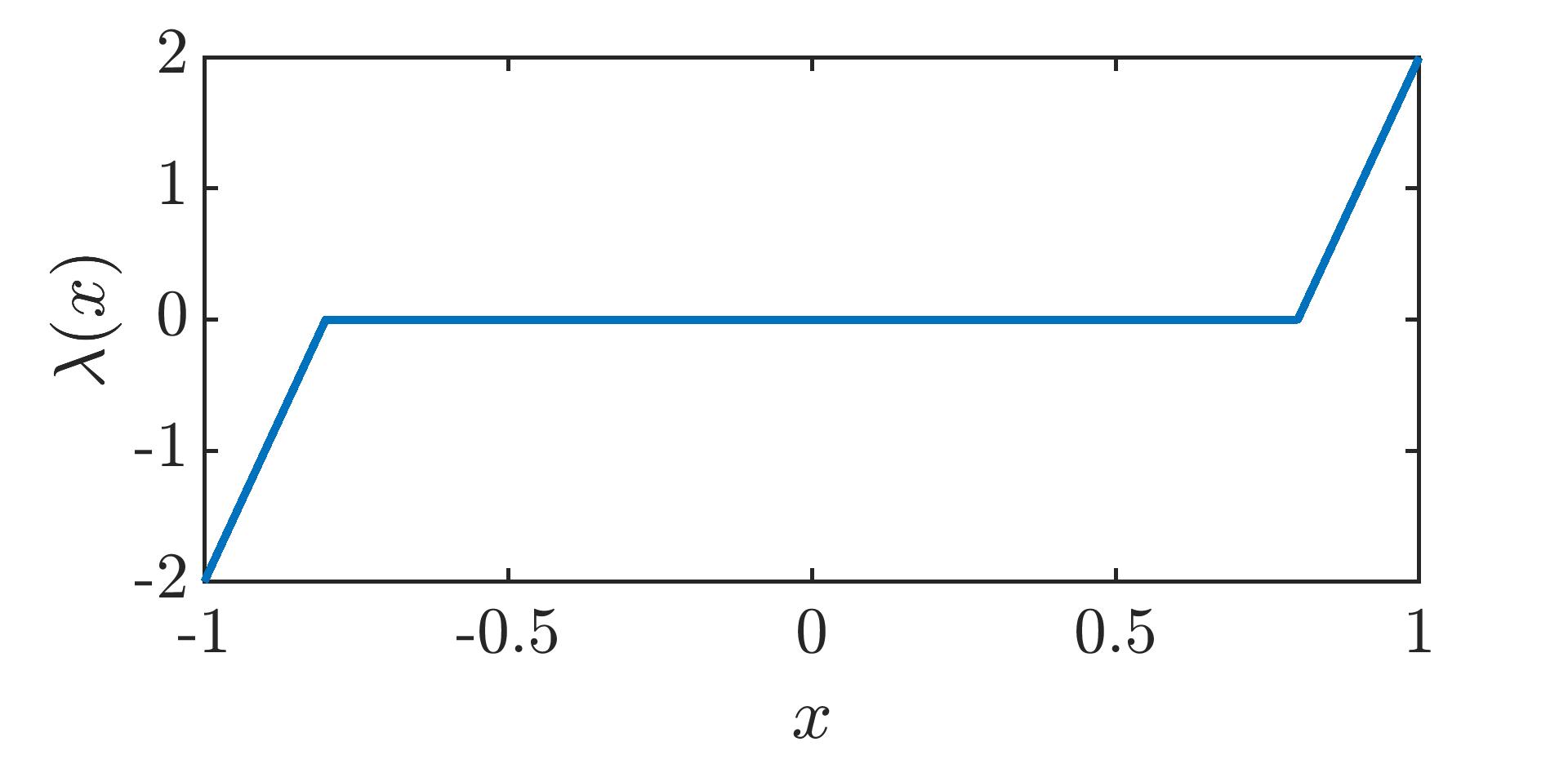
Figure 3: Demonstration of a shift function $\lambda(x^{\star})$ for $K_{H}^{(3,2)}$ with $H(x^{\star})=0.1$ on the domain $\Omega=[-1,1]$.

3.3 Knot Matrix Examples

Typical examples of knot matrices corresponding to the case of $r+1=3$ B-splines of order $\ell=2$ are given by

$$\mathbf{T}_{\rm Left}=\begin{bmatrix}-4&-3&-2\\ -3&-2&-1\\ -2&-1&0\end{bmatrix},\;\;\;\mathbf{T}_{\rm Sym}=\begin{bmatrix}-2&-1&0\\ -1&0&1\\ 0&1&2\end{bmatrix},\;\;\;\mathbf{T}_{\rm Right}=\begin{bmatrix}0&1&2\\ 1&2&3\\ 2&3&4\end{bmatrix},$$

where $\mathbf{T}_{\rm Left}$ and $\mathbf{T}_{\rm Right}$ denote the biased filters used for filtering at the left and right boundaries of the domain, respectively. The symmetric kernel $T_{\rm Sym}$ is used in the interior of the domain.

3.4 Kernel coefficients

To determine the coefficients, $c_{\gamma},$ the post-processing filter must satisfy consistency and moment conditions. These are equivalent to polynomial reproduction:

Consistency + $r$ Moments		Polynomial Reproduction
$\int_{\mathbb{R}}\,K_{\mathbf{T}}(x)\,dx=1$	$\Rightarrow$	$\int_{\mathbb{R}}\,K_{\mathbf{T}}(x-y)\,dy=1$
$\int_{\mathbb{R}}\,K_{\mathbf{T}}(x)x^{k}\,dx=0,\quad 1\leq k\leq r$	$\Rightarrow$	$\int_{\mathbb{R}}\,K_{\mathbf{T}}(x-y)y^{k}\,dy=x^{k},\,k\in\mathbb{Z},\quad 1\leq k\leq r$

where $r$ is the number of moments. This aids in ensuring that the accuracy of the underlying data is not destroyed. For non-symmetric kernels the knot matrices can change with each filtering point $x^{\star}$, and so the kernel coefficients need to be recomputed with every convolution evaluation, which is not the case in the interior. The polynomial reproduction requirement

$$K_{\mathbf{T}}\star x^{p}=x^{p},\;\;\;p=0,\ldots,r,$$

can be expressed as

$$\sum_{\gamma=0}^{r}c_{\gamma}(x^{\star})\int_{\mathbb{R}}B^{\ell}_{\mathbf{T}_{\gamma}}(y)(x-y)^{p}\;dy=x^{p},\;\;\;p=0,\ldots,r.$$

Choosing $x=0$ results into a linear system

$$\begin{bmatrix}b_{0,0}&\ldots&b_{0,r}\\ \vdots&&\vdots\\ b_{r,0}&\ldots&b_{r,r}\end{bmatrix}\begin{bmatrix}c_{0}\\ c_{1}\\ \vdots\\ c_{r}\end{bmatrix}=\begin{bmatrix}1\\ 0\\ \vdots\\ 0\end{bmatrix}$$ (8)

where

$$b_{p,\gamma}=\int_{\mathbb{R}}B^{\ell}_{\mathbf{T}_{\gamma}}(y)(-y)^{p}\;dy\;\;\text{for}\;\;p,\gamma=0,\ldots,r.$$

Solving the linear system (8) yields the kernel coefficients. More explicit formulas for the coefficient system (8) in the uniform symmetric knot matrix case are provided in [22], while the general knot matrix case is considered in [23, 24].

$\lambda=-2$	$\lambda=0$	$\lambda=2$

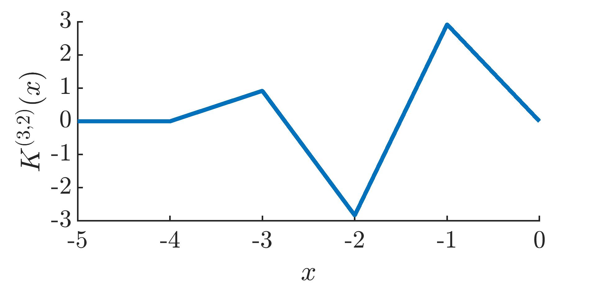
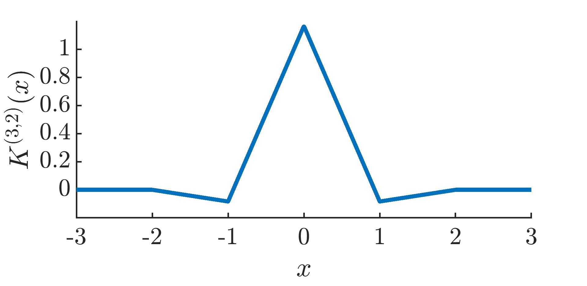
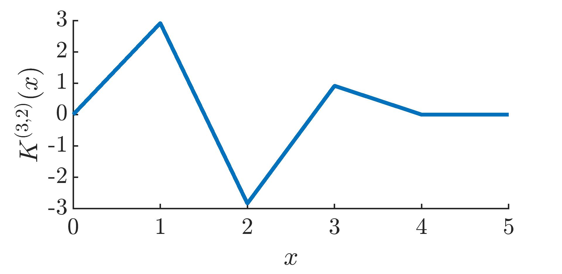
Figure 4: Shifted Kernels for $K^{(3,2)}(x)$. For $\lambda=\pm 2$, $x=0$ corresponds to the boundary. Note that owing to the reflection of $y$ in the kernel argument during the convolution, $\lambda=-2$ ($\lambda=2$) corresponds to the left-sided (right-sided) kernel in the physical space.

3.5 Generalized Spline Kernels

An issue arising from position-dependent filters is that errors increase in boundary regions for FEM data and in the case of PIC denoising, resulting into the failure to preserve boundary layers. In the past these issues have been addressed by using larger numbers of B-splines or convex combinations of SIAC kernels [21, 25], but as detailed in [18], adding a single generalized spline can decrease errors at the boundaries without increasing the kernel support. For example, near the left boundary, write

$$K_{H\,\mathbf{T}}(x)=\sum_{\gamma=0}^{r}c_{\gamma}(x)B^{\ell}_{H\,\mathbf{T}_{\gamma}}(x)+c_{r+1}B^{\ell}_{H\,\mathbf{T}_{r+1}}(x).$$

Here the coefficients are still determined by requiring polynomial reproduction. The new knot matrices are defined based off the sign of $\lambda$ by

$$\lambda<0\rightarrow\begin{bmatrix}\mathbf{T}\\ \mathbf{s}_{L}\end{bmatrix},\;\;\lambda=0\rightarrow\mathbf{T},\;\;\lambda>0\rightarrow\begin{bmatrix}\mathbf{s}_{R}\\ \mathbf{T}\end{bmatrix}.$$

Here the $1\times(\ell+1)$ knot sequences for the left and right generalized splines are given by

$$\mathbf{s}_{L}=\Big{[}\lambda+\frac{1}{2}(r+\ell)-1,\lambda+\frac{1}{2}(r+\ell),\ldots,\lambda+\frac{1}{2}(r+\ell)\Big{]},$$

and

$$\mathbf{s}_{R}=\Big{[}\lambda-\frac{1}{2}(r+\ell),\ldots,\lambda-\frac{1}{2}(r+\ell),\lambda-\frac{1}{2}(r+\ell)+1\Big{]}.$$

For instance, consider the case of $r=2$ and $l=2$. The new left and right knot matrices for $K^{(3,2)}_{H}$ are given by

$$\mathbf{T}_{Left}=\begin{bmatrix}-4&-3&-2\\ -3&-2&-1\\ -2&-1&0\\ -1&0&0\end{bmatrix},\;\;\;\mathbf{T}_{Right}=\begin{bmatrix}0&0&1\\ 0&1&2\\ 1&2&3\\ 2&3&4\end{bmatrix}.$$

Plots of the these boundary kernels are given in Fig. 5.

$\lambda=-2$	$\lambda=2$

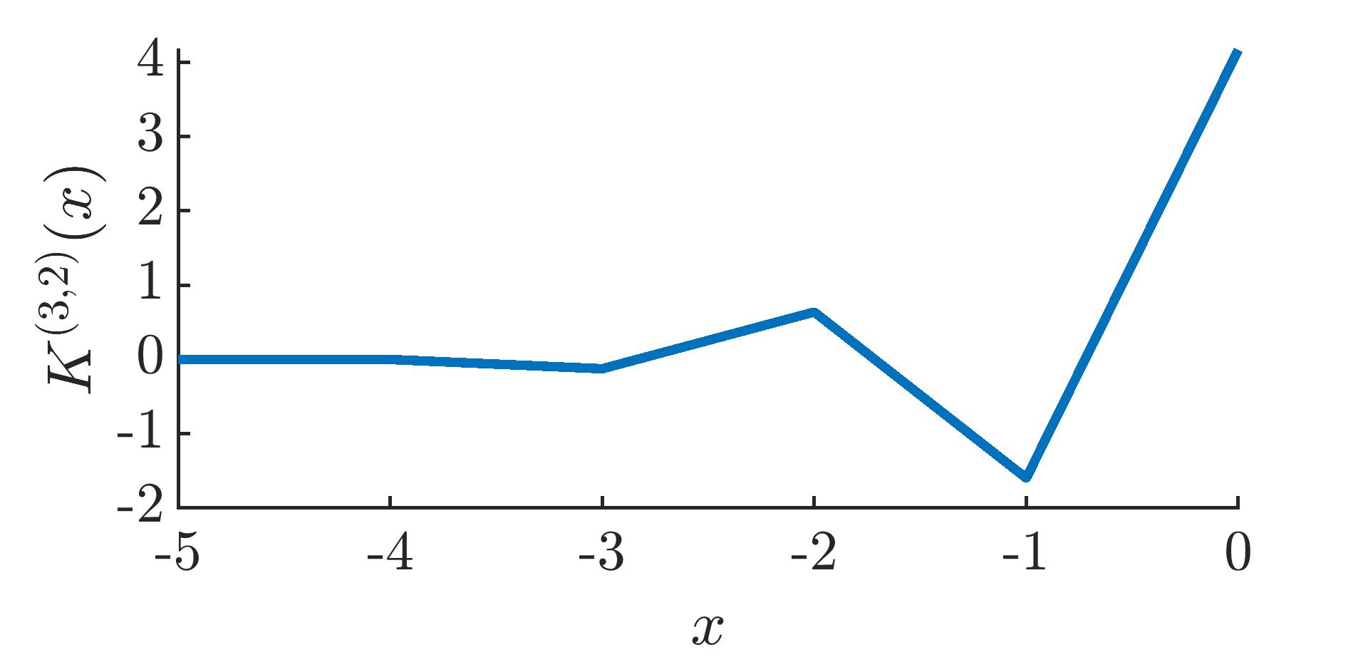
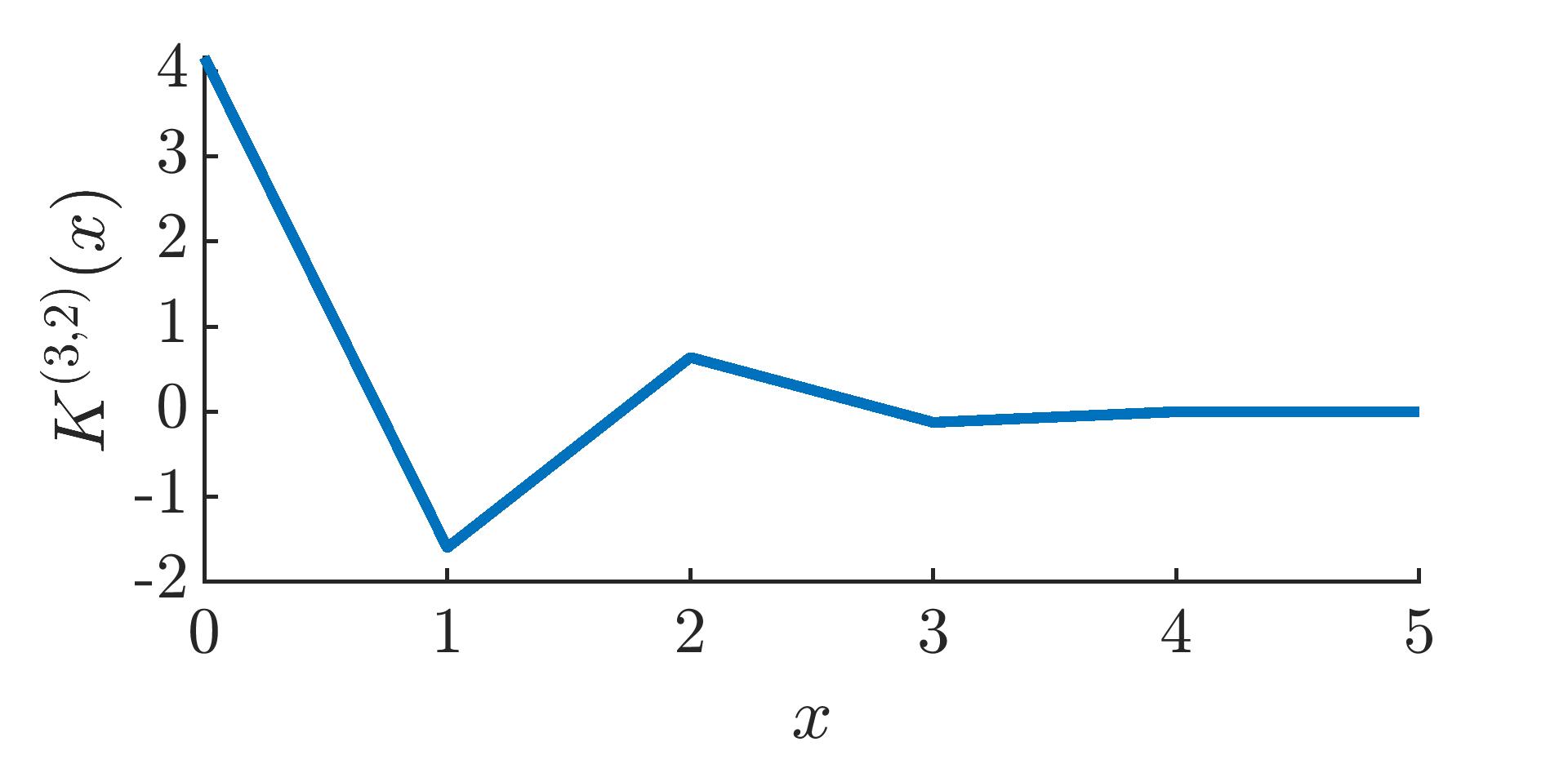
Figure 5: Shifted Kernels for $K^{(3,2)}(x)$ including a generalized spline. Here $x=0$ corresponds to a boundary.

3.6 Adaptive kernel scaling

Although the addition of generalized splines improves the performance of SIAC denoising for moderate kernel scalings, as will be observed in the numerical results, some care is needed to preserve short-duration sharp gradients near boundaries when the kernel scaling becomes large. To that end, we propose a remedy via an adaptive kernel scaling given by

$$H_{\rm adaptive}(x)=\begin{cases}H_{\rm int},\;&x-H_{\rm int}\frac{r+\ell}{2}\geq a\;\text{ and }\;x+H_{\rm int}\frac{r+\ell}{2}\leq b,\\ \frac{h_{\rm grid}}{r+\ell}+2(x-a)\frac{H_{\rm int}-h_{\rm grid}/(r+\ell)}{H_{\rm int}(r+\ell)},\;&x-H_{\rm int}\frac{r+\ell}{2}\leq a,\\ \frac{h_{\rm grid}}{r+\ell}+2(x-b)\frac{-H_{\rm int}+h_{\rm grid}/(r+\ell)}{H_{\rm int}(r+\ell)},\;&x+H_{\rm int}\frac{r+\ell}{2}\geq b,\end{cases}$$ (9)

where $H_{\rm int}$ is a large scale desired for the interior, and $h_{\rm grid}$ is the size of the mesh elements. $H_{\rm int}$ is typically related to the physical length scale in the problem. This choice of adaptive scaling provides the advantage of preserving the boundary values of the underlying initialization by reducing the kernel support to a single element at the boundary locations. This enables the polynomial-reproduction property of the kernel to be maintained. Fig. 6 shows a depiction of this adaptive scaling and its smoothing effect on the transition between the symmetric kernel and the position-dependent kernel with a shifting parameter. This adaptive scaling has the additional effect of creating a smoother shifting function $\lambda$ and thereby resulting in a smoother transition between different knot matrices.

3.7 Convolution evaluation

The consistent evaluation of convolution in 1D requires keeping track of all the breaks in continuity of the approximation and breaks in differentiability of the kernel within the scaled kernel support. By only integrating between these breaks in continuity of the data or the kernel, the convolution can be performed exactly using Gaussian quadrature. A detailed discussion of the implementation can be found in Docampo-Sánchez et al. [26].

3.8 Fourier representation

As our primary focus is to denoise PIC data, it is critical to examine the Fourier transform of the convolution kernel to quantify the damping effect applied to each frequency. This examination will guide the choice of the kernels when denoising moments. Unfortunately, analytical computation of the kernel’s Fourier response is only possible in the periodic case for the symmetric kernel with a constant kernel scaling. In such a case, the Fourier representation of the SIAC kernel composed of $(r+1)$ B-splines of order $\ell$ and constant scaling $H$ is given by

$$\hat{K}^{(r+1,\ell)}_{H}(k)=\left(\frac{\sin(\frac{kH}{2})}{\frac{kH}{2}}\right)^{\ell}\left(c_{{\lceil\frac{r}{2}\rceil+1}}+2\sum_{\gamma=1}^{{\lceil\frac{r}{2}\rceil}}\,c_{\gamma}\cos(\gamma kH)\right).$$ (10)

The first term in the product is controlled by the spline order, while the second is controlled by the number of B-splines, with the value of the coefficients, $c_{\gamma}$, being controlled by both the number of B-splines and the B-spline order.

In Fig. 7 the Fourier representation is displayed for varying kernel parameters. We observe that increasing the spline order, which corresponds to an increase in smoothness, causes the filter to sample smaller magnitude wave numbers more heavily and reduce oscillations. This makes sense as the Fourier transform of smoother functions decays faster and increasing the spline order results in a smoother kernel. Increasing the number of splines, which corresponds to increasing the number of moments, does not change the shape drastically, but slightly alters how the kernel samples different modes. Specifically, it flattens the Fourier response at $k=0$ by causing $\frac{d^{n}}{dk^{n}}\hat{K}^{(r+1,\ell)}(0)=0$ for $n=1,\ldots,r$. This follows from the polynomial reproduction condition on the kernel. Lastly, changing the scaling factor only causes a dilation in $k$ of kernel response and utilizes more (or fewer) elements in the filtering process. An understanding of the frequency effects of position-dependent and adaptively scaled filters remains an important area of further study. In particular, the standard methodology of computing the Fourier transform of the SIAC kernel is inappropriate owing to the spatial variability of the kernel function employed over the computational domain. One possible approach is the consideration of the spectrum of the discrete filtering operator, but that is beyond the scope of this work.

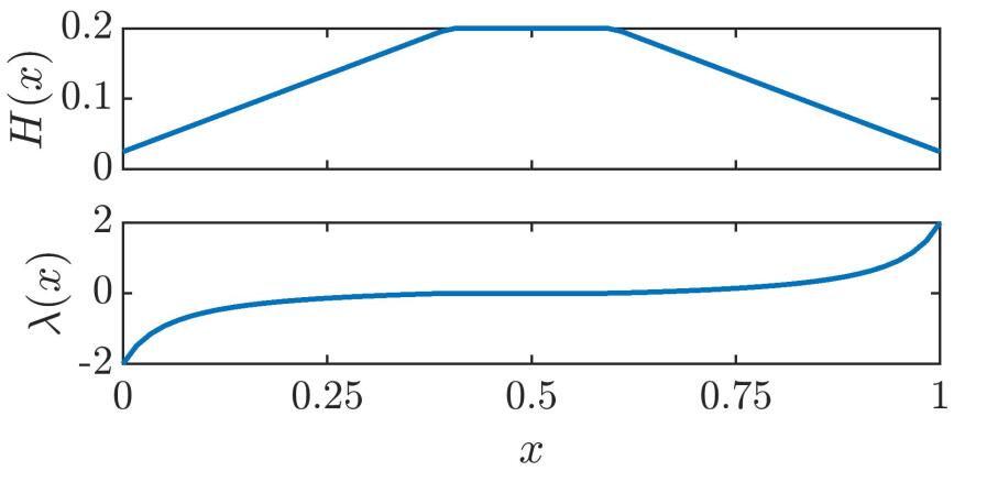
Figure 6: An adaptive kernel scaling example for $K^{(3,2)}(x)$ over the domain $\Omega=[0,1]$ with $H_{\rm int}=0.2$, $h_{\rm grid}=0.1$.

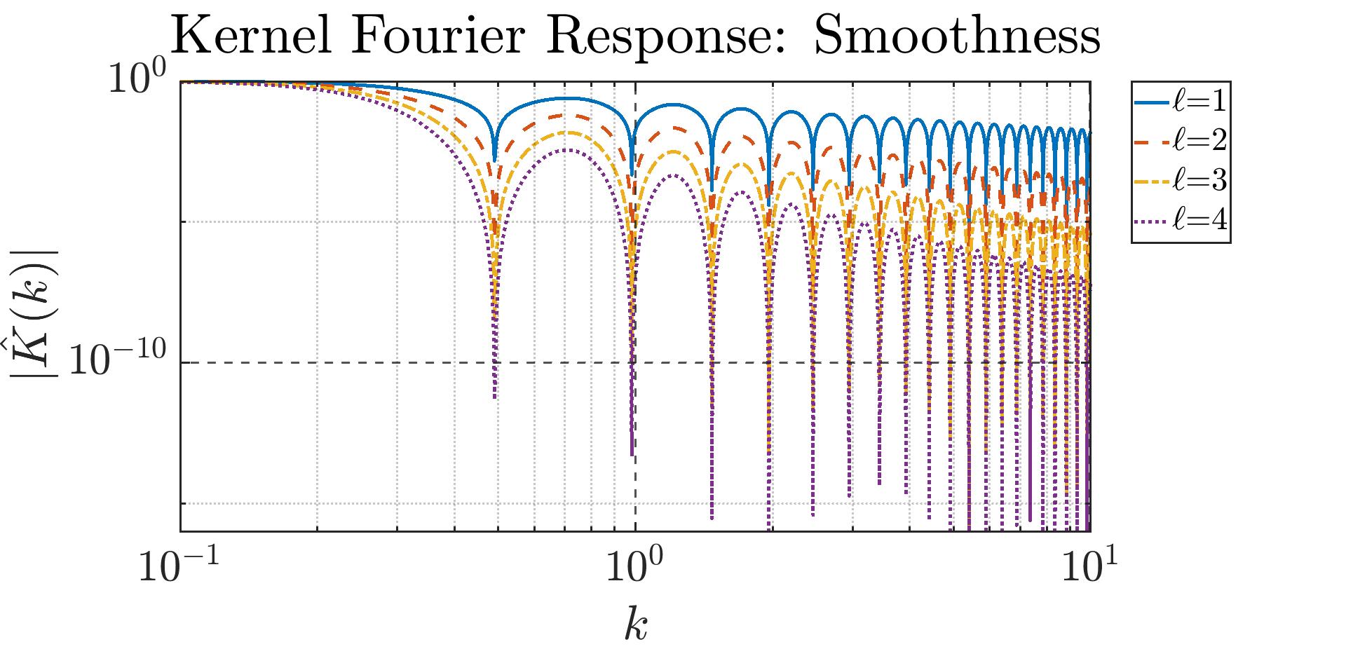
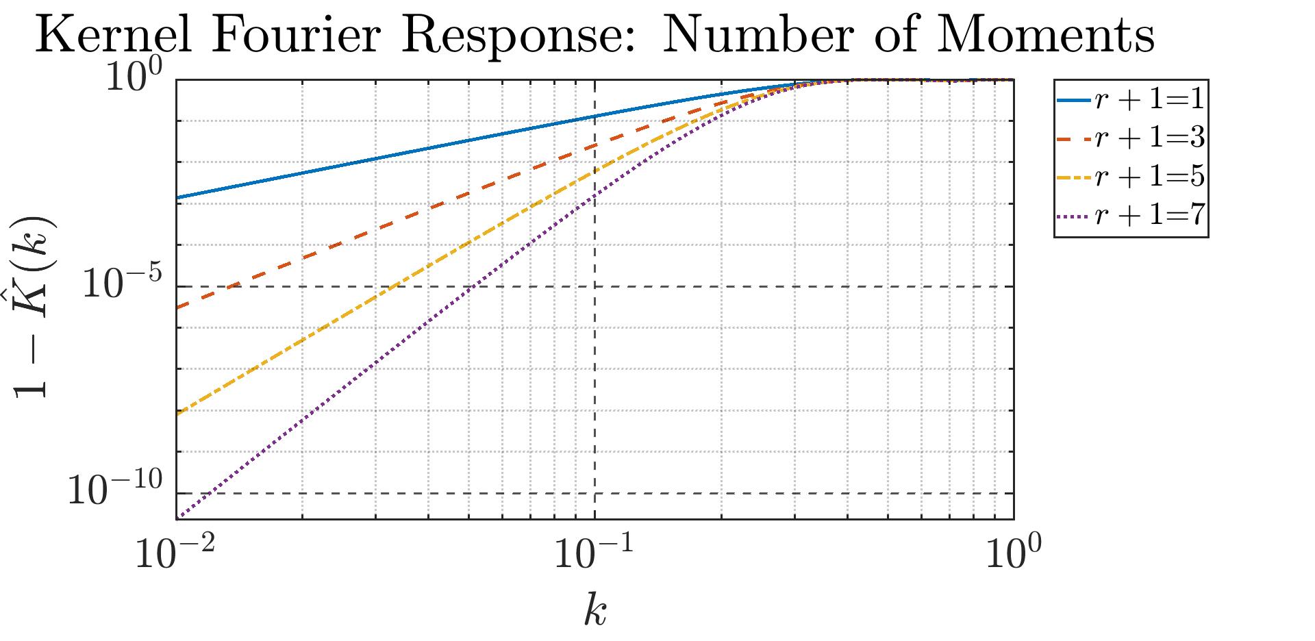
(a)		(b)

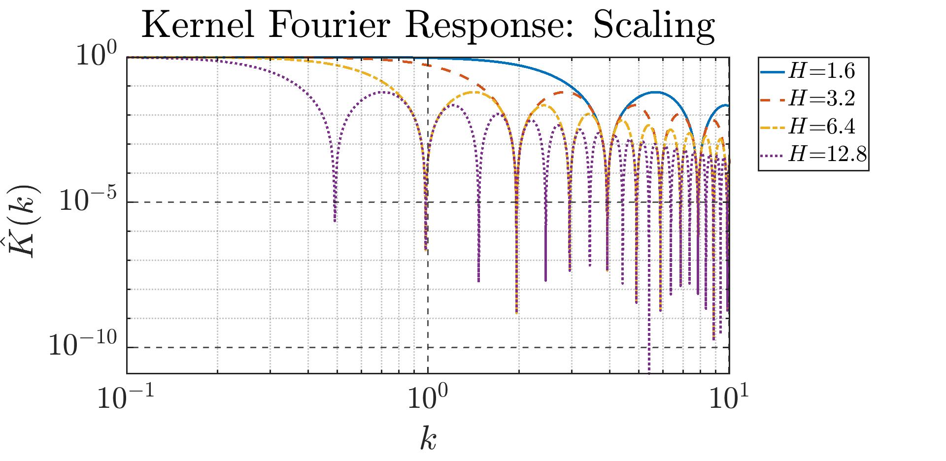
(c)

Figure 7: Variation of the magnitude of the analytic Fourier representation of the SIAC filter, $K^{(r+1,\ell)}_{H}$, with respect to (a) spline order ($\ell$), with higher orders corresponding to smoother and more diffused filtered data, (b) moment conditions ($r$), with more moment conditions allowing the capturing of more information about a point, and (c) kernel scaling ($H$), with a larger scaling resulting in more information being used in the filtering process. Note that the kernel is symmetric with respect to $k$ and that, unless indicated otherwise in the legends, $H=12.8$, $r+1=3$, and $\ell=2$.

4 Numerical Results

In this section the applications of the SIAC filter to denoise PIC data are considered. Here, both a periodic boundary condition and a boundary condition that introduces sharp gradients will be considered. For the former, an investigation of the damping of the noise using the uniformly scaled symmetric filter is done, where it is expected that the filter should preserve the physical oscillations. For the latter case, several aspects are studied, including comparisons of the abilities of position-dependent filters with or without generalized splines as well as with or without adaptive kernel scalings. The focus is if the boundary layers are resolved in the physical space and how that affects the Fourier space. It must be highlighted again that maintaining the boundary behavior of the data can be critical to obtaining accurate physics, e.g., for the Bohm criterion.

Given PIC moment data, there are three steps in the denoising procedure:

1. Construct a nodal piecewise interpolant as described in Sec. 2 for the given pointwise discrete data that is generated from a PIC simulation.

2. Select the kernel parameters ($r,\,\ell,$ and $H$), and filter the initialization obtained in Step 1 with the corresponding SIAC kernel. The choice of parameters depends on the type of data being filtered (characteristic length scales, desired damping effects, etc.).

3. Assess the filtered data from the point of view of physics

It was determined that there is an insensitivity in the initialization step to low polynomial degrees and therefore only results for a piecewise constant initialization are included in what follows.

Assessment of Fourier Effects

For the purposes of displaying the Fourier effects of the filtering procedure on the underlying data, plots of the single-sided amplitude spectrum are given. If the data is non-periodic, multiplication of the data vector by a Hanning window function is done in the first step to minimize any spectral leakage.

4.1 Periodic boundary conditions

The first test is for the possible effectiveness of the SIAC technique on denoising the PIC data. This requires the removal of high frequency/wavenumber (with wavelengths at cell size) noises and the preservation of physical oscillations. For this purpose, PIC simulations with periodic boundary conditions are considered. Such boundary conditions can be widely found in PIC simulations [27, 28] such as in the study of plasma instabilities [29, 30]. Here the data from the VPIC code [31] that simulates the whistler instability in magnetized plasma induced by the trapped electrons is used [32, 33]. For such periodic data, a symmetric SIAC filter with a constant kernel scaling over the whole domain can be used. Fig. 8 shows the results of applying the filtering procedure on periodic magnetic field data where the kernel is composed of 3 B-splines of order 2 ($r+1=3$, $\ell=2$). Here the domain is $\Omega=[0,1400]$ with a uniform grid spacing of $h_{grid}=\Delta x=0.1$, in the unit of Debye length $\lambda_{D}$. A large $H=64h_{grid}$ is chosen so that the truncated wavenumber is $k_{c}\tilde{<}\lambda_{D}^{-1}$.Choosing a small filter scaling, $H$, would result in less damping of the higher order modes as illustrated in Equation (10) and Fig. 7.

We first note that the Fourier modes match very well in the low frequency domain, resolving all the physical structures we are interested in. It is even more remarkable that the theoretical model of the kernel response matches very well with the observed damped frequencies in the Fourier space (the lower-left plot). As the analysis in Sec. 3.8 suggested, the damped frequencies are primarily controlled by the the kernel scaling $H$. Therefore, by choosing the kernel scaling appropriately, it is possible to target and damp noises with high wavenumbers while a good preservation of the real whistler waves peaked at $k\sim 0.1\lambda_{D}^{-1}$ is maintained, as seen from the Fourier spectrum.

This result suggests that for periodic data with limited sharp features SIAC filtering can be applied in an informed manner. The targeting physical frequency such as the whistler wave case is typically known a prior and can be readily used to guide the choice of $H$ in practice.

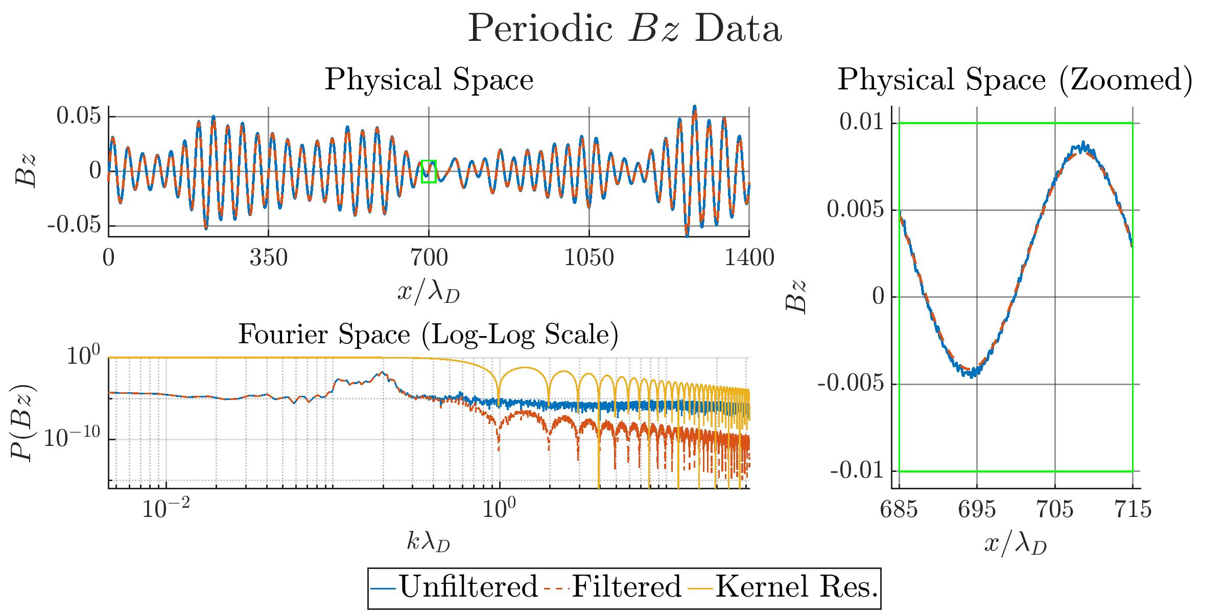
Figure 8: Application of SIAC filtering to periodic magnetic field for the whistler instability driven by the trapped electrons: (upper-left) filtered vs. unfiltered data over the whole domain. (right) zoomed-in physical space plot displaying spatial noise damping. (lower-left) single-sided amplitude spectrum of filtered and unfiltered data with analytic SIAC kernel response superimposed.

4.2 Data with sharp gradients near the boundary

The second test considers the capability of SIAC filtering to handle large gradients near the boundary. This can be a critical characteristic in some cases. Here the considered case is that of the non-neutral sheath (which forms near the region where a plasma intercepts a solid surface) that introduces sharp gradients to the plasma profiles; for instance see Fig. 9 and Fig. 11. It is worth noting that the electron conduction heat flux, $q_{n}^{e}$, in the form of its spatial gradient as shown in Eq. (4), plays an important role in setting the Bohm speed [5, 34], denoising of which is extremely demanding since itself suffers higher noise pollution than the plasma density and flow.

Here, position-dependent SIAC filters that include generalized splines and adaptive kernel scalings are used to denoise the data so that the Bohm criterion can be calculated. This avoids a long time average as proposed in Ref. [5], significantly reducing the computational cost.

The boundary behavior of the filtered data for varying kernel treatments is first examined in the physical space, shown in Fig. 9. It can be seen that the typical position-dependent filter composed of 3 B-splines of order 2 with a scaling of $H=32h_{grid}$ cannot preserve the boundary behavior of electron density. However, if a generalized spline is added to the position-dependent kernel to lend more weight to the filtering point in the weighted-average, it is possible to better maintain the boundary behavior. However, if we keep increasing the kernel support to $H=128h_{grid}$ while keeping all the other parameters the same, it can be observed that the generalized spline alone is not enough to maintain the boundary behavior. This is resolved by using the proposed adaptive kernel scaling given as Eq. (9), as confirmed in Fig. 9.

We then compare the single-sided amplitude spectrums of the filtered and unfiltered electron density data, results of which are shown in Fig. 10. While larger scalings are shown to have greater damping capabilities, there is not much of a disparity between the different boundary treatments using the same scaling. This makes sense as, while the differences in tracking the boundary behavior is apparent in physical space, only the data in a small portion of the domain near the boundary varies between these treatments. In aggregate, neither adaptive scalings nor generalized splines seem to matter as much as the choice of interior kernel scaling, when the spectrum of the filtered data is considered. Thus, the choice of boundary treatment may not be apparent in spectral analysis. The results in the Fourier space is largely comparable to the periodic case.

$H=3.2$	$H=12.8$
Without generalized splines, constant scaling	With generalized splines, constant scaling
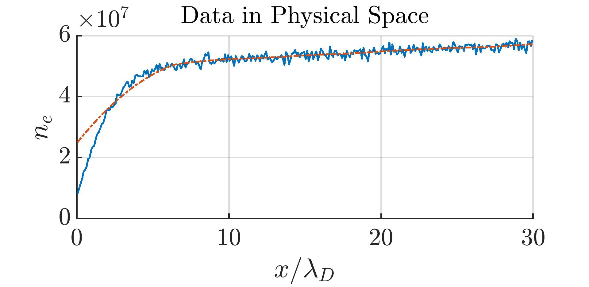
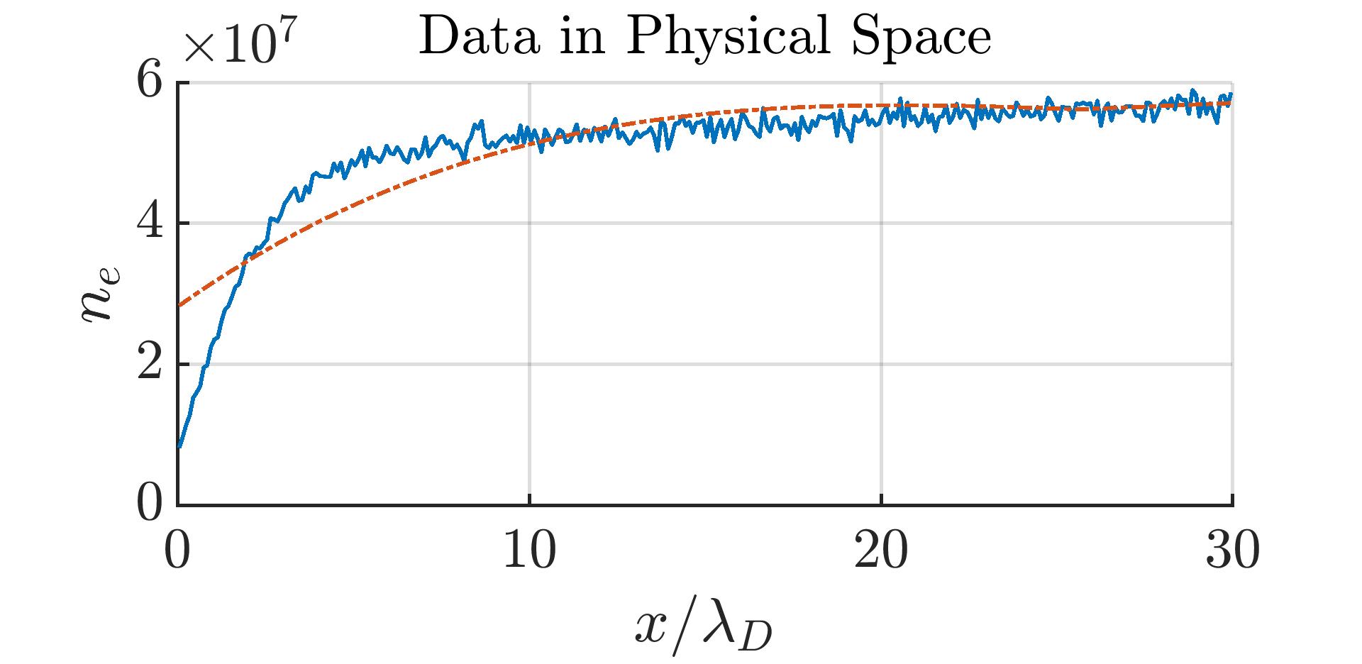
With generalized splines, constant scaling	With generalized splines and adaptive scaling

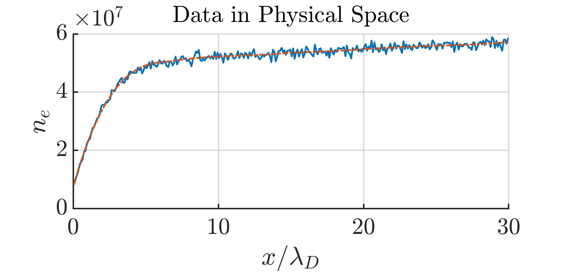
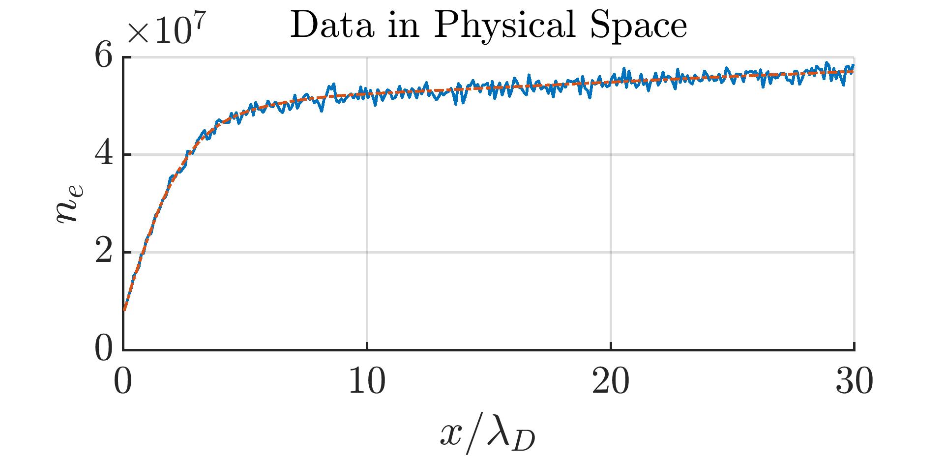
Figure 9: Effect of generalized splines and adaptive kernel scaling on boundary behavior preservation. The underlying data is electron density data $n_{e}$ with $\Omega=[0,800]$ and $h_{grid}=\Delta x=0.1$. Here the solid blue lines denote the unfiltered data and the dashed red lines the filtered data.

$H=3.2$	$H=12.8$
Without generalized splines, constant scaling	With generalized splines, constant scaling
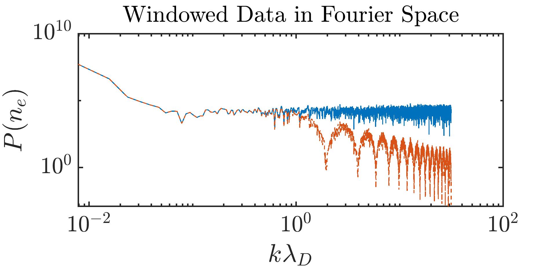
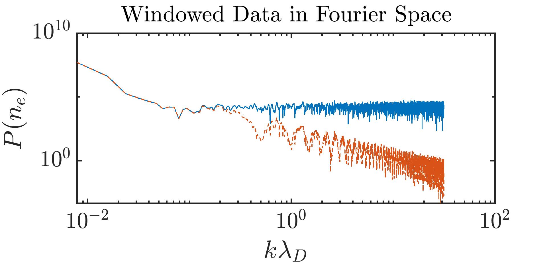
With generalized splines, constant scaling	With generalized splines and adaptive scaling

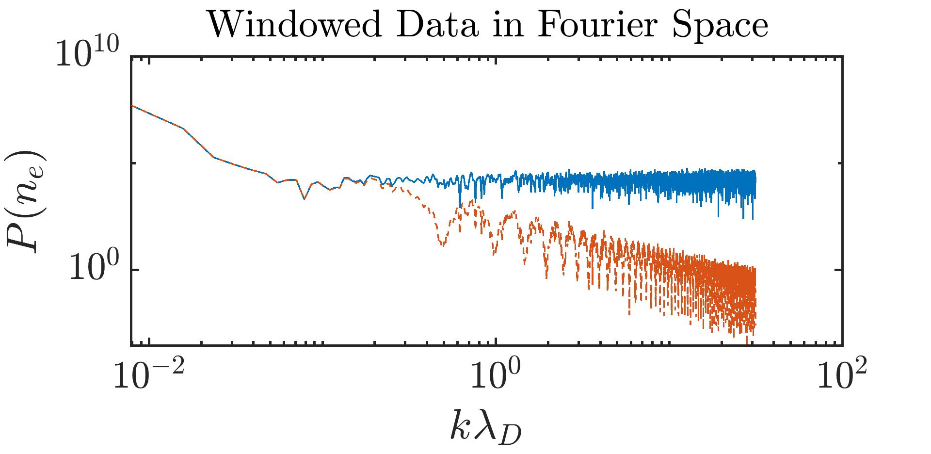
Figure 10: Effect of generalized splines and adaptive kernel scaling on the single-sided amplitude spectrum of electron density data $n_{e}$ with $\Omega=[0,800]$ and $h_{grid}=\Delta x=0.1$. Here the solid blue lines denote the unfiltered data and the dashed red lines the filtered data. Note that the underlying data was non-periodic so a Hanning window function was applied.

Next an investigation of the same choice of kernel parameters on the electron heat flux, $q^{n}_{e}$, and its spatial gradient, $dq^{n}_{e}/dx$, is performed. Note that here in the unfiltered case $dq^{n}_{e}/dx$ is computed by a central difference stencil of $q^{n}_{e}$ in the interior of the domain, and a 1st order biased stencil at the domain boundaries. The filtered derivative values are obtained by applying the same differencing procedure to the filtered $q^{n}_{e}$ values. Fig. 11 and Fig. 13 present the effect of the filtering scheme on $q^{n}_{e}$ and $dq^{n}_{e}/dx$ is shown. The data is found to be much more oscillatory than the electron density data, though the same behavior can be seen for $q^{n}_{e}$ under different filter parameters. Specifically, adding a generalized spline helps maintain boundary behavior for smaller $H$, but an adaptive scaling becomes neccessary for larger interior scalings. Similar behavior to the $n_{e}$ case is also observed in the single-sided amplitude spectra depicted in Fig. 12. With respect to the gradient of the heat flux, the differing boundary treatments are much less apparent in physical space (see Fig. 13). The presense of noise is particularly apparent in $dq^{n}_{e}/dx$ in that it oscillates rapidly about $0$, and much of the energy in the single-sided amplitude spectrum is contained in this noise manifesting in higher frequencies as depicted in Figure 13. The application of the filtering procedure serves to damp these higher frequencies. While it may appear that the choice of boundary treatment has little effect on $dq^{n}_{e}/dx$, in the next test, it will be seen that minor perturbations of this variable can have a large impact on computed quantities such as the Bohm speed.

This result suggests that the SIAC filters can be applied to the non-periodic data, capturing the information well in both the physical space (e.g., boundary layers) and Fourier space. It is particularly encouraging to observe the success in the Fourier space for an extremely noisy case of $dq^{n}_{e}/dx$.

$H=3.2$	$H=12.8$
Without generalized splines, constant scaling	With generalized splines, constant scaling
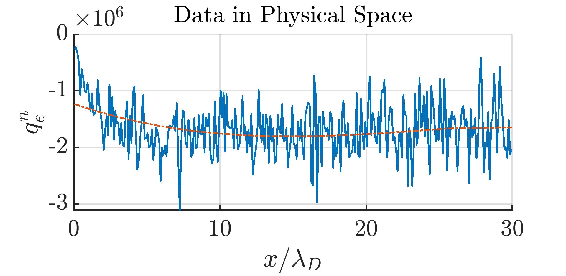
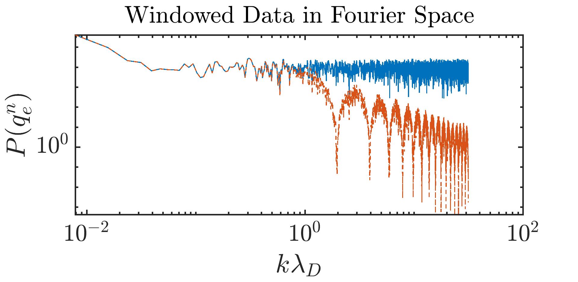
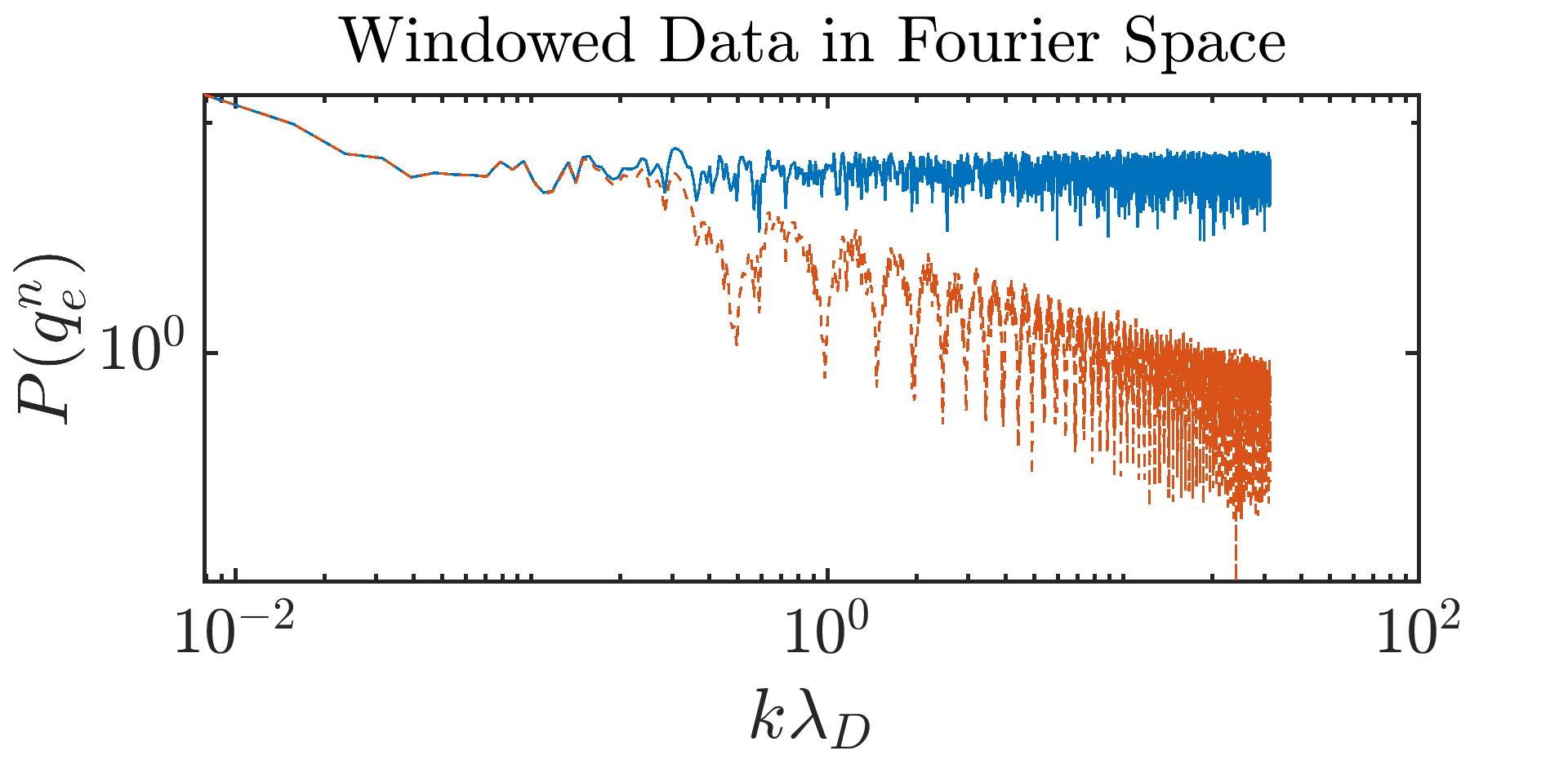
With generalized splines, constant scaling	With generalized splines and adaptive scaling

Figure 11: Effect of generalized splines and adaptive kernel scaling on boundary behavior preservation. The underlying data is electron heat flux data $q^{n}_{e}$ with $\Omega=[0,800]$ and $h_{grid}=\Delta x=0.1$. Here the solid blue lines denote the unfiltered data and the dashed red lines the filtered data.

$H=3.2$	$H=12.8$
Without generalized splines, constant scaling	With generalized splines, constant scaling
With generalized splines, constant scaling	With generalized splines and adaptive scaling

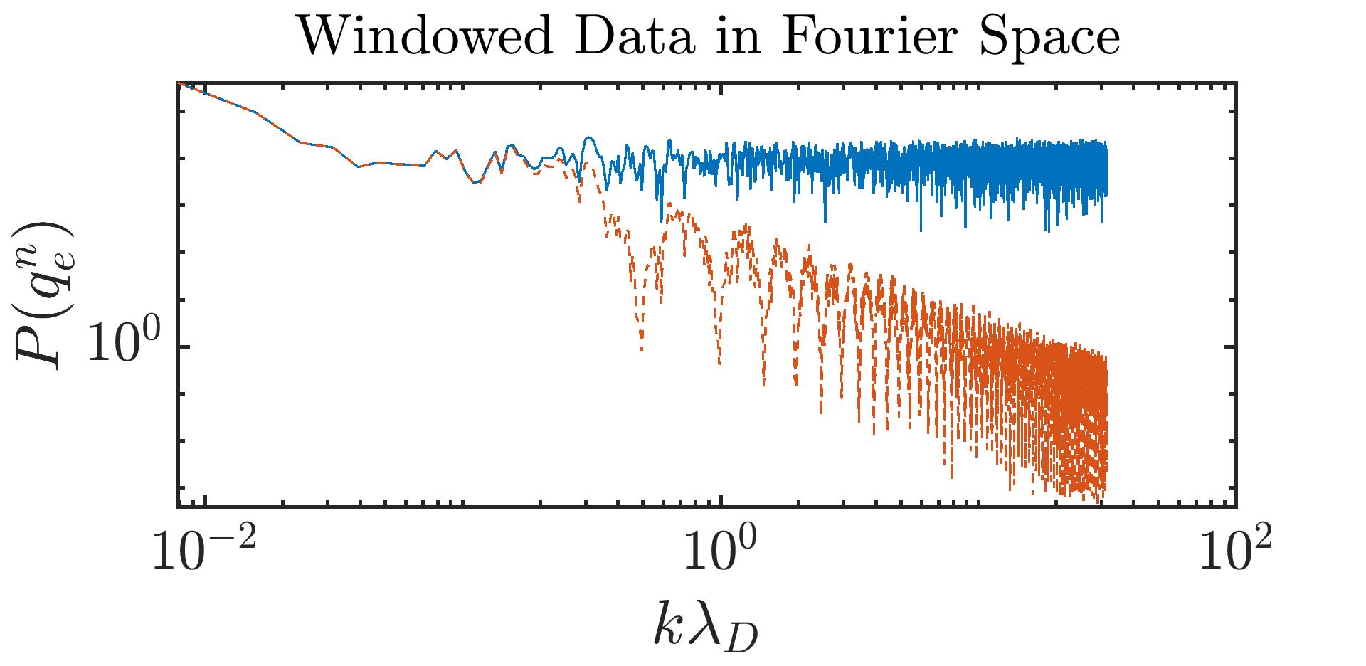
Figure 12: Effect of generalized splines and adaptive kernel scaling on the single-sided amplitude spectrum of electron heat flux data $q^{n}_{e}$ with $\Omega=[0,800]$ and $h_{grid}=\Delta x=0.1$. Here the solid blue lines denote the unfiltered data and the dashed red lines the filtered data. Note that the underlying data was non-periodic so a Hanning window function was applied.

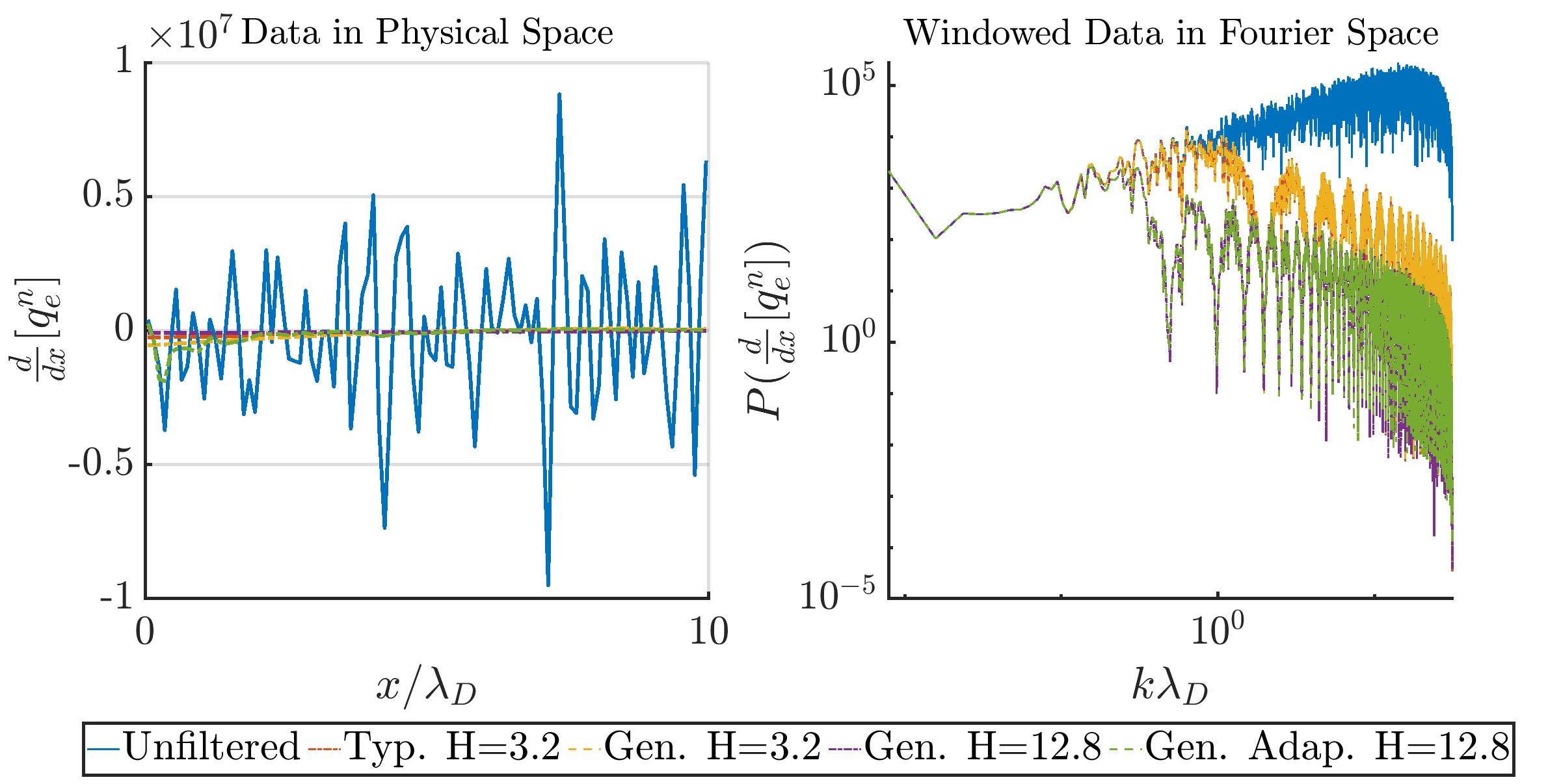
Figure 13: Effect of generalized splines and adaptive kernel scaling on electron heat flux gradient data $dq^{n}_{e}/dx$ in physical and frequency space. Here $\Omega=[0,800]$, $h_{grid}=\Delta x=0.1$, and the dashed red line (Typ.) denotes a filtering procedure with the typical kernel without generalized splines, while (Gen.) denotes a filtering with a kernel including a generalized spline. Finally, (Adap.) denotes that an adaptive kernel scaling is employed. In physical space, the effects of the differing boundary treatments are most apparent closest to the boundary, so the interior of domain is not shown. Note that the underlying data was non-periodic so a Hanning window function was applied for the spectrum computation.

4.3 Application to Bohm speed calculations

The numerical verification of the Bohm speed expression of Eq. (3) is a very challenging task. For instance, the Bohm speed is very sensitive to small perturbations in that if small perturbations like PIC noises in the data cause the denominator of Eq. (4) to flip signs or be near $0$, the computed Bohm speed can be either complex or blow-up. The contribution to such sensitivity of the Bohm speed to the noises are highly biased in the variables as seen from Eq. (4), where the electron heat flux gradient, $q_{n}^{e}$, contributes the most. On the other hand, $q_{n}^{e}$ itself has most of the noise due to it being the high moment calculated from the electron distribution. To mitigate such a challenge, Ref. [5] evolved to a static state solution in an excessively long time, collecting 200,000 snapshots of the static state solution. Their average is eventually used to verify the physical law sucessfully. Here we aim to show such an expensive brute-force strategy can be avoided by using a small amount of snapshots with the proposed SIAC filters.

Variable	$q_{n}^{e}$	$q_{n}^{i}$	$Q_{ee}$	$Q_{ei}$	$Q_{ii}$	$E$	$R_{T}$	$n_{e}$	$n_{i}$	$u_{ex}$	$u_{ix}$	$T_{ex}$	$T_{ix}$
$H$	8	4	16	16	16	2	32	6	6	8	8	16	4

Table 1: Variable specific scalings for 2,600 snapshots averaged data set found to produce qualitative agreement with respect to the long-time averaged data.

First, it is necessary to systematically examine the filtering requirements and choose proper scalings for each variable to retain the majority of the physics. Our idea behind these individualized variable scalings is to filter the short-time averaged variables, obtaining filtered data which qualitatively resembles the long-time averaged variables. Procedurally, this takes the form of replacing a single long-time averaged variable in the Bohm speed computation with a noisier short-time averaged counterpart, and then varying the kernel scaling of that short-time averaged variable until good qualitative agreement is obtained with respect to the long-time averaged variable and the long-time averaged Bohm speed. The number of snapshots, 2,600, is the minimum number of time steps for which this can be achieved for all variables. The discovered kernel scalings for each component is summarized in Tab. 1. Choosing the scalings in this manner allows for the preservation of the qualitative behavior of the data and real-valued Bohm speed calculations.

Unfiltered short-time averaged data
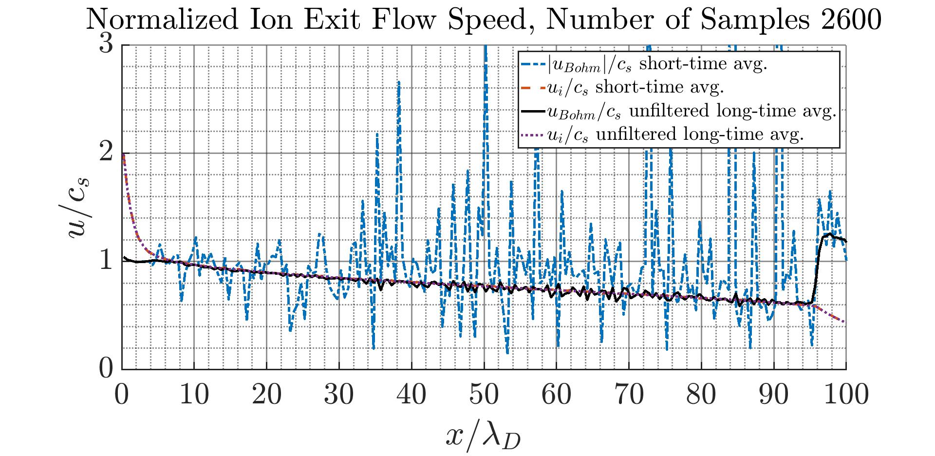
Filtered short-time averaged data

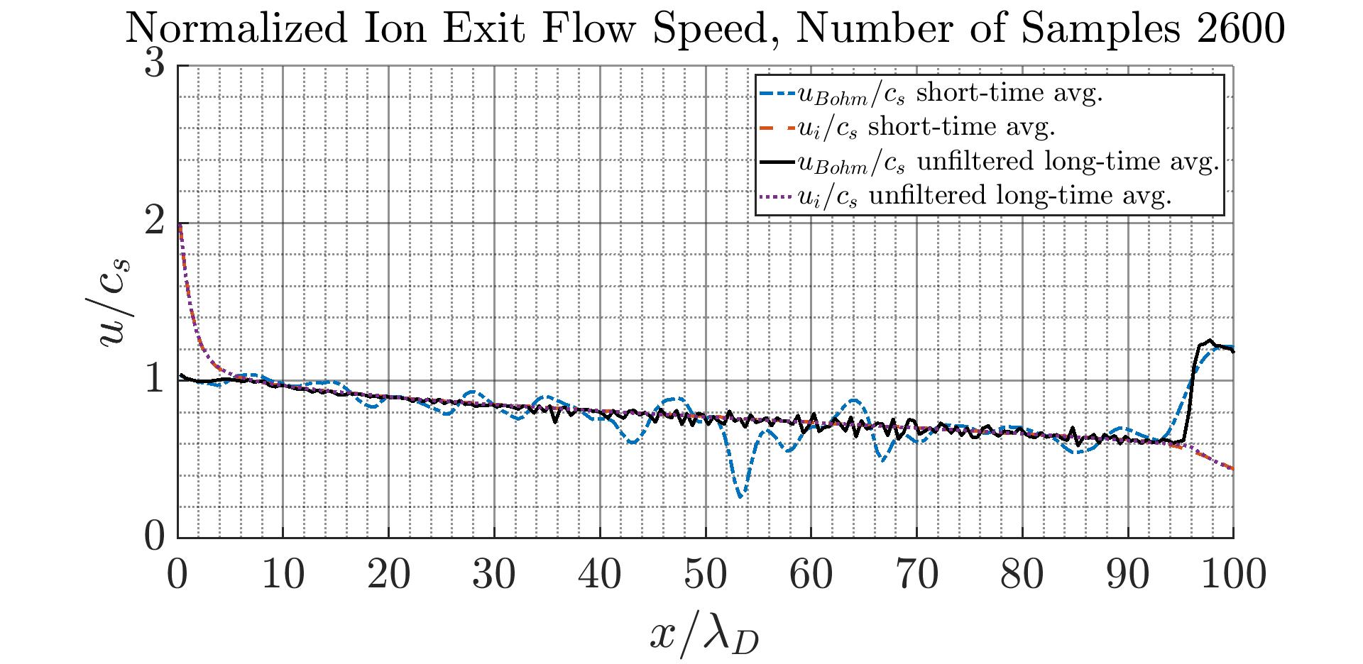
Figure 14: Comparison of Bohm speed and ion exit flow using filtered and unfiltered data time-averaged over 2,600 snapshots. The unfiltered long-time averaged data over 200,000 snapshots is also plotted. A $K^{(3,2)}_{H}$ kernel with scalings as indicated in Table 1 was used. Note that the modulus of $u_{Bohm}$ is plotted for the unfiltered short-time average data as the noise was sufficient to induce complex values.

Finally, when short-time averaged filtered data alone is used with the scalings chosen as indicated in Tab. 1, it is capable to obtain a desirable Bohm speed that tracks well with the long-time averaged calculations. This is shown in Fig. 14, where a comparison of the computed Bohm speed from the filtered and unfiltered data with all variables originating from a time average over 2,600 snapshots is shown. The unfiltered long-time averaged data over 200,000 snapshots is also plotted as a baseline. The lower plot of Fig. 14 shows that the filtered average of normalized Bohm speed (blue dash line) matches well with the long-time averaged value (solid black line) from [5].

This result shows that the proposed SIAC filters can be a promising data processing technique in a very practical PIC setting, which can potentially save significant computational cost. For instance, the presented study of Bohm speed suggests that the previous expensive 1D3V PIC simulation in [5] can be performed in a much shorter time (1.3%) to discover the same physical law.

5 Conclusions and Future Work

In this paper, the Smoothness-Increasing Accuracy-Conserving filters have been first-ever extended to effectively denoising discrete PIC data while preserving the underlying physics. Several aspects of the filters related to both the periodic boundary condition and a physical boundary condition that introduces the sharp gradient of plasma profiles have been investigated. Leveraging knowledge from SIAC applications in a FEM context, the position-dependent filters have been repurposed and a new adaptive scaling methodology has been developed. The proposed filter is assessed using the challenging task of uncovering physical laws, specifically the Bohm speed formulation. The outcomes show that the computational cost in PIC can be substantially reduced by reducing the macro-particle numbers or the time steps used for time-averaging. This underscores the substantial potential of the proposed filters as an effective tool for processing PIC data.

In the future, a more in-depth investigation of the sensitivity of the Bohm speed calculation to noisy variables will be investigated. One more vital capability of the filter that needs to be developed is to self-detect and resolve the interior structures possessing sharp gradients like the shocks, which is of great importance since the time-average approach does not apply to such a dynamical system. Additionally, quantifying the Fourier effects of the adaptively scaled and position-dependent filters will be done.

6 Acknowledgements

The first author would like to thank the LANL LDRD ISTI Student fellow program and, along with the fourth author, the AFOSR under grant number FA9550-20-1-0166 which enabled this work, as well as Dr. Ayaboe Edoh for his insights. This work was partially supported by the U.S. Department of Energy SciDAC partnership on Tokamak Disruption Simulation between the Programs of Fusion Energy Sciences (FES) and Advanced Scientific Computing Research (ASCR). It was also partially supported by Mathematical Multifaceted Integrated Capability Center (MMICC) of ASCR. Los Alamos National Laboratory is operated by Triad National Security, LLC, for the National Nuclear Security Administration of U.S. Department of Energy (Contract No. 89233218CNA000001). The authors wish to acknowledge and thank Dr. Yuzhi Li for providing the PIC data on which the Bohm speed calculations were based.

References

- Krall and Trivelpiece [1973] N. A. Krall, A. W. Trivelpiece, Principles of Plasma Physics, McGraw-Hill Book Company, 1973.
- Hockney and Eastwood [1988] R. W. Hockney, J. W. Eastwood, Computer Simulation Using Particles, Taylor & Francis, 1988.
- Birdsall and Langdon [1985] C. K. Birdsall, A. B. Langdon, Plasma Physics via Computer Simulation, McGraw-Hill Book Company, 1985.
- Zhang et al. [2023] Y. Zhang, J. Li, X. Tang, Cooling flow regime of a plasma thermal quench, Europhysics Letters 141 (2023) 54002.
- Li et al. [2022] Y. Li, B. Srinivasan, Y. Zhang, X. Tang, Bohm criterion of plasma sheaths away from asymptotic limits, Physical Review Letters 128 (2022) 085002.
- Bohm [1949] D. Bohm, The characteristics of electrical discharges in magnetic fields, Qualitative Description of the Arc Plasma in a Magnetic Field (1949).
- Nguyen et al. [2020] T. Nguyen, G. Chen, L. Chacón, An adaptive em accelerator for unsupervised learning of gaussian mixture models, arXiv preprint arXiv:2009.12703 (2020).
- Chen et al. [2021] G. Chen, L. Chacón, T. B. Nguyen, An unsupervised machine-learning checkpoint-restart algorithm using gaussian mixtures for particle-in-cell simulations, Journal of Computational Physics 436 (2021) 110185.
- Dimits and Lee [1993] A. Dimits, W. W. Lee, Partially linearized algorithms in gyrokinetic particle simulation, Journal of Computational Physics 107 (1993) 309–323.
- Parker and Lee [1993] S. Parker, W. Lee, A fully nonlinear characteristic method for gyrokinetic simulation, Physics of Fluids B: Plasma Physics 5 (1993) 77–86.
- Ricketson and Cerfon [2016] L. F. Ricketson, A. J. Cerfon, Sparse grid techniques for particle-in-cell schemes, Plasma Physics and Controlled Fusion 59 (2016) 024002.
- Muralikrishnan et al. [2021] S. Muralikrishnan, A. J. Cerfon, M. Frey, L. F. Ricketson, A. Adelmann, Sparse grid-based adaptive noise reduction strategy for particle-in-cell schemes, Journal of Computational Physics: X 11 (2021) 100094.
- Denavit [1972] J. Denavit, Numerical simulation of plasmas with periodic smoothing in phase space, Journal of Computational Physics 9 (1972) 75–98.
- Wang et al. [2011] B. Wang, G. H. Miller, P. Colella, A particle-in-cell method with adaptive phase-space remapping for kinetic plasmas, SIAM Journal on Scientific Computing 33 (2011) 3509–3537.
- Gassama et al. [2007] S. Gassama, É. Sonnendrücker, K. Schneider, M. Farge, M. O. Domingues, Wavelet denoising for postprocessing of a 2d particle-in-cell code, in: ESAIM: Proceedings, volume 16, EDP Sciences, 2007, pp. 195–210.
- Bramble and Schatz [1977] J. H. Bramble, A. H. Schatz, Higher order local accuracy by averaging in the finite element method, Mathematics of Computation 31 (1977) 94–111.
- Ryan and Shu [2003] J. Ryan, C.-W. Shu, On a one-sided post-processing technique for the discontinuous Galerkin methods, Methods and Applications of Analysis 10 (2003) 295–308.
- Ryan et al. [2015] J. K. Ryan, X. Li, R. M. Kirby, K. Vuik, One-sided position-dependent Smoothness-Increasing Accuracy-Conserving (SIAC) filtering over uniform and non-uniform meshes, Journal of Scientific Computing 64 (2015) 773–817.
- Jallepalli et al. [2019] A. Jallepalli, R. Haimes, R. M. Kirby, Adaptive characteristic length for L-SIAC filtering of FEM data, Journal of Scientific Computing 79 (2019) 542–563.
- C. de Boor [1978] C. de Boor, A Practical Guide to Splines, volume 27 of Applied mathematical sciences, Springer New York, 1978.
- van Slingerland et al. [2011] P. van Slingerland, J. K. Ryan, C. Vuik, Position-dependent Smoothness-Increasing Accuracy-Conserving (SIAC) filtering for improving discontinuous Galerkin solutions, SIAM Journal on Scientific Computing 33 (2011) 802–825.
- Mirzargar et al. [2016] M. Mirzargar, J. K. Ryan, R. M. Kirby, Smoothness-Increasing Accuracy-Conserving (SIAC) filtering and quasi-interpolation: A unified view, Journal of Scientific Computing 67 (2016) 237–261.
- Peters [2015] J. Peters, General spline filters for discontinuous Galerkin solutions, Computers & Mathematics with Applications 70 (2015) 1046–1050.
- Nguyen and Peters [2016] D.-M. Nguyen, J. Peters, Nonuniform discontinuous Galerkin filters via shift and scale, SIAM Journal on Numerical Analysis 54 (2016) 1401–1422.
- Ji et al. [2014] L. Ji, P. van Slingerland, J. K. Ryan, K. Vuik, Superconvergent error estimates for position-dependent Smoothness-Increasing Accuracy-Conserving (SIAC) post-processing of discontinuous galerkin solutions, Mathematics of Computation 83 (2014) 2239–2262.
- Docampo-Sánchez et al. [2020] J. Docampo-Sánchez, G. Jacobs, X. Li, J. Ryan, Enhancing accuracy with a convolution filter: What works and why!, Computers & Fluids 213 (2020) 104727.
- Birdsall and Langdon [2018] C. K. Birdsall, A. B. Langdon, Plasma physics via computer simulation, CRC press, 2018.
- Hockney and Eastwood [2021] R. W. Hockney, J. W. Eastwood, Computer simulation using particles, crc Press, 2021.
- Pritchett [2000] P. L. Pritchett, Particle-in-cell simulations of magnetosphere electrodynamics, IEEE transactions on plasma science 28 (2000) 1976–1990.
- Verboncoeur [2005] J. P. Verboncoeur, Particle simulation of plasmas: review and advances, Plasma Physics and Controlled Fusion 47 (2005) A231.
- Bowers et al. [2008] K. J. Bowers, B. Albright, L. Yin, B. Bergen, T. Kwan, Ultrahigh performance three-dimensional electromagnetic relativistic kinetic plasma simulation, Physics of Plasmas 15 (2008) 055703.
- Guo and Tang [2012] Z. Guo, X.-Z. Tang, Ambipolar transport via trapped-electron whistler instability along open magnetic field lines, Physical Review Letters 109 (2012) 135005.
- Zhang and Tang [2023] Y. Zhang, X.-Z. Tang, On the collisional damping of plasma velocity space instabilities, Physics of Plasmas 30 (2023) 030701.
- Tang and Guo [2016] X.-Z. Tang, Z. Guo, Critical role of electron heat flux on bohm criterion, Physics of Plasmas 23 (2016) 120701.