Redback: A Bayesian inference software package for electromagnetic transients

Abstract

Fulfilling the rich promise of rapid advances in time-domain astronomy is only possible through confronting our observations with physical models and extracting the parameters that best describe what we see. Here, we introduce Redback; a Bayesian inference software package for electromagnetic transients. Redback provides an object-orientated python interface to over 12 different samplers and over 100 different models for kilonovae, supernovae, gamma-ray burst afterglows, tidal disruption events, engine-driven transients, X-ray afterglows of gamma-ray bursts driven by millisecond magnetars among other explosive transients. The models range in complexity from simple analytical and semi-analytical models to surrogates built upon numerical simulations accelerated via machine learning. Redback also provides a simple interface for downloading and processing data from Swift, Fink, Lasair, the open-access catalogues, and BATSE and fit this or private data. Redback can also be used as an engine to simulate transients for telescopes such as the Zwicky Transient Facility and Vera Rubin with realistic cadences, limiting magnitudes, and sky-coverage or a hypothetical user-constructed survey with arbitrary settings. We also provide a more general simulation interface suitable for target of opportunity observations with different telescopes. We demonstrate through a series of examples how Redback can be used as a tool to simulate a large population of transients for realistic surveys, fit models to real, simulated, or private data, multi-messenger inference and serve as an end-to-end software toolkit for parameter estimation and interpreting the nature of electromagnetic transients.

1 Introduction

Rapid advances in electromagnetic telescope sensitivity and survey capabilities are revolutionising transient astronomy. However, to realise the full promise of the rich and large photometric data sets, we need a robust toolkit for simulating what we expect to see, building and exploring our models and fitting the observations. Such advancements can enable us to ultimately learn the physics that drives these transients, optimise our survey strategies and instruments, and gain insights into the lives and afterlives of stars and the evolution of our Universe. Such a tool must also be modular and open-source to be easily adaptable to an individual user’s needs and easily maintain and upgrade.

Here, we introduce Redback an open-source, end-to-end Bayesian Inference software package for simulating and fitting electromagnetic transients. Redback provides an object-orientated python interface to multiple sampling algorithms, models for several different electromagnetic transients, an interface to download and process the data for multiple transients from various catalogues, simulate transients for real surveys such as the Large Synoptic Survey of Space and Time (LSST) (Ivezić et al., 2019) and Zwicky Transient Facility (ZTF) (Bellm et al., 2019) and fit the observations through Bayesian inference. Redback is also built on modern python, with many adopted practices to aid continual development, continuous integration, a large library of unit tests and examples which ensure that the primary features of Redback remain stable through future development.

There have been several iterations of an open-source software with at least some similar aims and capabilities e.g., MOSFiT (Guillochon et al., 2018), NMMA (Pang et al., 2022), 3ML (Vianello et al., 2015), Haffet (Yang & Sollerman, 2023), SNCosmo (Barbary et al., 2022), and SNANA (Kessler et al., 2009). However, these previous software packages are limited in different ways e.g., a limited library of models or sampling algorithms, engines to simulate transients but not perform inference or vice versa, inflexible interface to not allow a user to change the likelihood or the model or fit a different data type, stale development teams or built on software practices that do not align with modern software development. Redback provides several advantages over other software packages and mitigate the aforementioned issues:

• A large library of inbuilt models and a simple interface for users to add their own. Several models implemented in Redback are direct improvements to previous models, or model transients that one can not model in other packages.

• An engine to both simulate realistic transients for surveys and target of opportunity observations, and perform inference i.e., a tool to validate an entire inference workflow or optimise surveys.

• A modular and flexible interface, users can easily swap likelihoods, models, plotting without ever modifying the source code.

• Simple interface to over 12 different open-source samplers, enabling cross-sampler validation or use of samplers that are better tuned for transient inference or have additional capabilities such as multiprocessing.

• A large and active development team, particularly regarding sampling functionality, which is facilitated by the interface to Bilby (Ashton et al., 2019; Romero-Shaw et al., 2020) and other open-source software.

This paper is intended to describe the capabilities and mark the version 1.0 release of Redback. We note that Redback has been open-source and distributed under the GPL licence since March 2022 and earlier versions of Redback have already been used in previous publications (e.g., Sarin et al., 2020a, b; Sarin et al., 2021, 2022a, 2022b; Sarin & Lasky, 2022; Schulze et al., 2023; Levan et al., 2023; Sarin & Metzger, 2023). This paper is structured as follows: In Sec. 2 we describe the design philosophy of Redback, how the different parts of the software interact, and the $3$ typical workflows we expect Redback to be used for. In Sec. 3, we describe the different modules in Redback and how they are used in various workflows. In Sec. 4, we show the interface for Redback, in particular how to download and process data, setting up the inference workflow, plotting methods and simulating transients. This basic interface is followed by more detailed examples in Sec. 5 and 6 where we demonstrate the different capabilities of Redback. In particular, we first show how Redback can be used to jointly analyse a multi-messenger binary neutron star signal with X-ray and gravitational-wave data, and then to fit different types of real electromagnetic transients. In Sec. 7 we briefly describe features in Redback that will be added in future releases and conclude in Sec. 8.

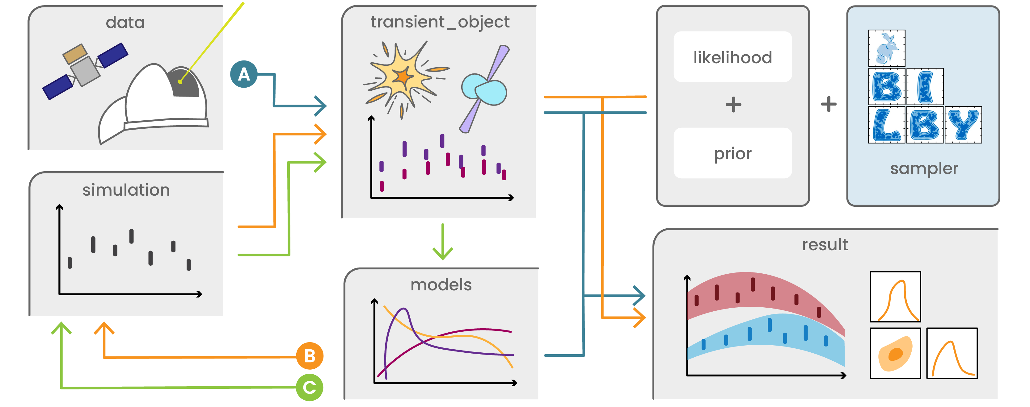
Figure 1: Flowchart showcasing the different modules of Redback and how they interact for different workflows.

2 Design Philosophy

The driving aim for Redback is to be truly modular, with the flexibility to adapt to the different requirements/preferences of end-users and for users to use different parts of the software without requiring additional overhead or modifying the source code. Similarly, users should be able to replace an entire model with their own python function, or make minor changes to different aspects such as the distribution of ejecta or the recipe to relate kilonova parameters to binary parameters in a kilonova model without the need to dig into the source code. Models must also have minimal dependencies and not depend on other aspects of the software, enabling users to evaluate a model as they would any other python function. Second, Redback must be flexible to both serve as a workhorse in expert workflows in transient astronomy and as an accessible tool for newcomers to the field. For example, advanced users must be able to change the default likelihood, the prior for the model, the model itself, how plots look, and how the data is processed without digging into the source code, requiring a flexible interface. However, more novice users should not need to make these choices and should be able to fit their favourite transient with just a few lines of code.

With these driving aims in mind, all primary modules of Redback are built as python classes which can be easily replaced or modified by the users and do not depend on other objects in Redback. This enables advanced users to change or replace the different Redback modules for their desired workflows and functionality, while the choices are made by default for more novice users. In Fig.1 we show the different modules of Redback and how they interact for the $3$ most common workflows we expect this software to be used for.

• A: Fitting a real transient. We anticipate that one of the most common use cases for Redback will be fitting data of a real astrophysical transient. This workflow will typically involve getting data from one of the catalogues using the get_data module in Redback, or users can provide their own private data. The user will then use this data to create a Transient object which loads the data in a homogeneous format and can be used for plotting the data or additional processing such as converting flux data to luminosity. The user then passes this Transient object along with a string referring to a model from transient_models or their own python-wrapped model, a prior module, a likelihood module and a string referring to a sampler that is available in Bilby (Ashton et al., 2019; Romero-Shaw et al., 2020) to perform fitting through Bayesian inference and obtain a result object. The result object contains the posterior, and other properties such as the Bayesian evidence. This result class can also be used to make plots such as the fitted lightcurve, the corner plot, or the cumulative distribution function of all parameters. We emphasise that for the novice user, choices like the likelihood and prior are made by default, but more advanced users can make changes to these as they desire.

• B: Fitting a simulated transient. Many users will also fit simulated data as both verification of the inference workflow or to predict constraints from mock observations. In this workflow, the user would start with a model from transient_models or supply their own model. Then use the simulation object to create synthetic data. After the creation of this simulated data, the workflow for fitting is the same as workflow A.

• C: Simulating a transient or a population of transients. Users may also wish to create a population of transients, for example to understand how many afterglows LSST will see in a year or to understand selection effects of surveys. These workflows require choosing a model from transient_models or supplying a python-wrapped model and passing this to the simulation module alongside a prior object which describes the distribution of each parameter in the model that constitutes the population. Complex prior constraints can be placed on this population through the use of prior_constraints.

The above briefly describes how different modules in Redback interact for different workflows. We now give a general overview of the Redback software and describe in detail each module, its capabilities and how it can be modified. Redback is installable via pip and available at https://github.com/nikhil-sarin/redback.

3 Software Overview

Redback is built on a class structure and almost every aspect of the software exists as an independent python class. Here we describe each of these different modules and their primary functionality. We stress that these modules are standalone and can be used independently to adapt to different needs and workflows, or modified or replaced to provide additional functionality.

3.1 Data

Redback provides an interface to download and process data from multiple catalogues through the get_data module. In particular, this includes the flux, flux density or the photon arrival time data for gamma-ray bursts (GRBs) detected by the Neil Gehrels Swift Observatory available at Swift Data Centre (Evans et al., 2010), the magnitude or flux density data of transients from ZTF from LASAIR (Smith et al., 2019) or Fink (Möller et al., 2021) which in the future are expected to also host transient lightcurves from LSST (Ivezić et al., 2019), the archival GRB data from BATSE (Fishman et al., 1994) and compilation of optical transient lightcurves available at the Open Access Catalog (OAC) (Guillochon et al., 2017).

For each of the above catalogues, the get_data module provides a one line interface to download and process the data into a pandas data frame and save it as a human-readable file in an appropriate location to integrate with the rest of Redback. This module also attempts to find additional metadata such as the redshift of the transient, the GRB photon index, T$90$ among other properties and process the data to add additional attributes such as the integrated flux, flux density and their respective errors.

As the data is stored as human-readable file and readable as a pandas data frame, the user can easily add additional private data or verify and modify any erroneous data. The get_data can be used independently of all other parts of Redback and may be used to simply process a large quantity of transient data from public archives.

3.2 Transient classes

The primary unifying module of Redback are the Transient classes. These are separated into two main types, a generic transient class which is applicable for any type of transient and an optical transient class. These classes serve as parent classes for five other classes; prompt, afterglow, kilonova, supernova, and tde which provide a more seamless interface for the specific type of transient, any additional processing such as converting the flux data to a luminosity and modify some default behaviour, such as labels for plotting, where plots are saved etc. We note that the afterglow class is further split into a short and long GRB class but these are functionally equivalent and only differ in locations of metadata.

For all transient classes, we provide one-line class methods to load the data from different catalogs obtained via the get_data module, or from the simulation module (described in Sec 3.4). The Transient objects can also be initialised independently of any class method by specifying the observed properties. In Sec. 4.2, we show how to initialise these Transient objects for different workflows.

All transient objects also have two important attributes; data_mode and use_phase_model. The former is an attribute which dictates what Redback assumes to be the mode of data for the transient e.g., magnitude for magnitude data, while the latter is a Boolean switch which dictates whether the transient has observed times in reference to a known start time (as usually the case for an afterglow) or is in Modified Julian Days (MJD) without a reference (as usually the case for most other transients). Again, these attributes affect choices such as the labels for plotting and where plots are saved but also in some cases the default likelihood used by Redback.

3.3 Models

While the most desirable method would be to confront observations with the best models that include the most physics (typically hydrodynamical and radiative transfer simulations), such models are not tractable for fitting given the demanding computational requirements of Bayesian inference (each model must be evaluated over a range of parameters at least $\mathcal{O}(10^{4})$ times to fit a typical transient). To be tractable for inference, all models in Redback are either analytical, semi-analytical, or surrogates built with machine learning from numerical simulations. The latter are provided by another standalone software package redback_surrogate that is available independently but we consider as part of the Redback software stack. Here, we describe the models for various different transients available in Redback and how they can be modified.

To remain true to our driving aim of modularity, all models are callable python functions and can be called on an arbitrary set of values with minimal dependencies. These functions can all be easily modified through the use of dependency injection (described in Sec 3.3.15) without needing modify the Redback source code or replaced entirely within the rest of the workflow with a user-provided model. Most Redback models can provide outputs in different formats e.g., luminosity, integrated flux, magnitude or flux density enabling them to be used to fit any type of data format. For magnitude and integrated flux data, Redback will integrate the spectrum and calculate the band pass magnitude/flux. This behaviour could be easily modified to use a flux density to magnitude conversion to further alleviate computational demands. We note that this behaviour is enabled by default for afterglow models where the effect of assuming a flux density to magnitude conversion as opposed to integrating a band pass is minimal.

3.3.1 Broadband GRB afterglow

Gamma-ray bursts are typically followed by lower energy broadband emission referred to as afterglow (e.g., Sari et al., 1998). The broad consensus is that the afterglow is a product of the relativistic jet interacting with the ambient interstellar medium, an interaction that produces synchrotron emission. However, there are several aspects of afterglow models that are ill-understood, such as the jet structure, i.e., the distribution of energy as a function of angle, or the role of reverse shocks, or additional emission components, or energy injection.

Redback provides an interface to several different afterglow models. For example, the different jet-structure models implemented in afterglowpy (Ryan et al., 2020), and implementations of several other physical models described in the literature (Sari et al., 1998, 1999; Gottlieb et al., 2018; Lamb et al., 2020; Lamb et al., 2021). For each of the models, users can make additional modifications to the physics such as the inclusion of jet spreading, inverse Compton emission, and energy injection or more specific settings such as the resolution of the integration scheme. For other models, users can choose the exact jet-structure profile, whether the interstellar medium is at a constant density or a wind-like medium etc., and whether the shock is refreshed. All these modifications are handled through additional optional keyword arguments in the python function which allows the advanced users to make changes as they wish while more novice users can avoid having to make these decisions.

Alongside these physically-motivated models we also include some purely phenomenological broken power-law models with different degrees of components. In total, Redback includes $21$ physically-motivated afterglow models in addition to the five phenomenological models, providing coverage of the different physical assumptions involved in afterglow modelling and to test the robustness of inferred models across different modelling assumptions.

3.3.2 Broadband kilonova afterglow

Similar to a GRB afterglow, there also exists an expectation for synchrotron emission when the slower moving kilonova ejecta interacts with the ambient interstellar medium. However, unlike models for the GRB afterglow, where we are aided by decades of observations, there are currently no confident detections of a kilonova afterglow. Nevertheless, we provide an interface to several different kilonova afterglow models described previously in the literature (Nakar & Piran, 2011; Sarin et al., 2022b) and make modifications to some of GRB afterglow models described above to be more suited for a kilonova afterglow (e.g., Gottlieb et al., 2018; Ryan et al., 2020). In the future, we will add kilonova afterglow models more representative of the ejecta distribution we see in numerical simulations (Kathirgamaraju et al., 2019; Nedora et al., 2021).

3.3.3 Kilonovae

The revolutionary observations of AT2017gfo (e.g., Abbott et al., 2017b; Abbott et al., 2017a; Arcavi et al., 2017; Kasen et al., 2017; Coulter et al., 2017; Villar et al., 2017) provided definitive evidence of a thermal transient powered by r-process nucleosynthesis. However, despite the extensive observations and significant theoretical model development, many aspects of kilonovae remain uncertain. In Redback we provide implementations of $18$ different kilonova models which range in complexity and implemented physics. Many aspects of these models such as the distribution of ejecta mass or the recipe to relate the binary neutron star (BNS) or neutron star black hole (NSBH) parameters to kilonova parameters can be changed through the use of dependency injection (described in Sec. 3.3.15).

The simplest kilonova model implemented in Redback is a one component kilonova model (Villar et al., 2017). Although minimal in parameters and quick to evaluate and therefore fit to observations, this model has already been shown to be unsuccessful in explaining multiple aspects of kilonovae observations. To address the inability of such a simple model to explain observations, we also provide implementations of two and three component kilonova models following Villar et al. (2017) and implementations of MOSFiT kilonova models (Cowperthwaite et al., 2017; Villar et al., 2017). These models all effectively ignore the dynamics of the ejecta, assuming the entire ejecta component is moving at one velocity, an assumption that is likely incorrect. We therefore also provide models where the ejecta is distributed into shells which expand homologously, similar in spirit to the model presented in Metzger et al. (2010) and Metzger (2019). Alongside this, we also provide an interface to the heating-rate kilonova models (Korobkin et al., 2012; Hotokezaka & Nakar, 2020; Dorsman et al., 2023), which allow the user to describe the velocity and opacity distribution themselves.

The above models all have parameters that describe the kilonova ejecta properties itself i.e., the mass and velocity of the ejecta. However, it has become increasingly common for kilonova models to be built upon the BNS or NSBH parameters which are then related to the ejecta parameters with a series of recipes from numerical relativity simulations. We provide several implementations of these models including models for BNS and NSBH, including for example the BNS model implemented in MOSFiT (Nicholl et al., 2021) which includes additional physics such as shock cooling to describe the early optical lightcurve (Piro & Kollmeier, 2018), or implementations of models presented in Coughlin et al. (2019).

While the above models are all semi-analytical, we also provide $3$ models that are machine-learning surrogates to numerical simulations. These surrogates are provided in the optional package redback_surrogate (described in more detail below), and are implementations of surrogates built in KilonovaNet (Lukošiute et al., 2022). In the future, we will continue to add more kilonovae models (Banerjee et al., 2020; Korobkin et al., 2021) and allow greater flexibility to existing models such as changing the calculation of the thermalisation efficiency.

3.3.4 Supernovae

Redback contains many supernova models of varying levels of complexity. Most of the models have both a bolometric implementation and an implementation for multi-band photometry. This setup allows the user to fit bolometric luminosity, magnitude, integrated flux, or flux density data. Similar to MOSFiT where physics such as the interaction process, photosphere, and spectral energy distribution (SED) can be swapped, Redback supernovae models can do the same since they are implemented using dependency injection. For all models, these aspects are chosen by default corresponding to the physics implemented but can be swapped without modifying the source code for a different module to capture different physics.

The simplest model, such the exponential-power law model, is purely phenomenological and built upon no physics in terms of luminosity but assumes a diffusive photosphere with a temperature floor, and a blackbody SED. Other models are more physically motivated such as several variations of the Arnett model (Arnett, 1980, 1982) for ⁵⁶Ni-powered supernovae including a version which also incorporates shock cooling, a version that incorporates line absorption for modeling Type Ia supernovae, and a version which incorporates synchrotron emission for modeling type Ic supernovae. Then there are models for circumstellar (CSM) interaction powered supernovae (Chatzopoulos et al., 2013) as well as a mix of CSM and ⁵⁶Ni power. We also include other models similar to those available in MOSFiT, such as the basic magnetar, slsn, and magnetar+nickel models (Nicholl et al., 2017; Guillochon et al., 2018), as well as new models which include non-vacuum dipole spin-down (Lasky et al., 2017) and ejecta acceleration from the pulsar wind nebula (Sarin et al., 2022b; Omand & Sarin, 2023).

Again, through the use of dependency injection, these models can be easily modified to capture different physics. We also provide an interface to supernova models implemented in SNCosmo (Barbary et al., 2022), which further amplifies the library of supernovae models available in Redback. In future releases, we will be adding surrogate models to hydrodynamical/radiative transfer simulations of interaction powered supernovae, among other models.

3.3.5 Engine driven transients

Distinct from the magnetar-driven supernovae models described above, we also provide a general class of magnetar driven models. Such models aim to capture the emission that would be produced in a magnetar-driven kilonova or a magnetar-driven fast blue optical transient (Drout et al., 2014; Arcavi et al., 2016). Several different models are implemented such as those that capture the dynamical evolution of the nascent neutron star (Sarin et al., 2022b) or the dynamical evolution of the ejecta (Metzger & Piro, 2014; Sarin et al., 2022b). We also include models with relativistic considerations (Yu et al., 2013; Sarin et al., 2022b), non-vacuum dipole spin (Lasky et al., 2017), and models with variation in their treatment of the thermalisation efficiency or gamma-ray leakage (Wang et al., 2015; Sarin et al., 2022b). We also include an implementation of the trapped magnetar model that has been suggested as an explanation for the enigmatic fast X-ray transient, CDF-S XT1 (Sun et al., 2019). In the future, we will add models to capture energy injection from fallback accretion onto a central black hole.

3.3.6 Millisecond magnetar

Ever since the launch of Neil Gehrels Swift Observatory (Gehrels et al., 2004), the origin of the X-ray afterglows of gamma-ray bursts has been a long source of debate. In particular, features referred to as the internal and external plateaus are difficult (although not impossible) to explain within the standard picture of synchrotron emission from a jet interacting with the ambient medium. These plateaus are readily explained as the bare or processed spin down from a highly magnetic, rapidly rotating newly born neutron star i.e., a millisecond magnetar.

In Redback, we provide several implementations of millisecond magnetar models, such as early models which assumed the neutron star only spun down through vacuum dipole radiation (Zhang & Mészáros, 2001; Rowlinson et al., 2013), to extensions that included a variable braking index (Lasky et al., 2017). We also provide models which include a collapse time (Sarin et al., 2020a), to capture lightcurves when the neutron star undergoes a delayed collapse to a black hole. The above models all implicitly assume that the observed emission is a constant factor of the real spin-down power of the neutron star. In reality, it is difficult to assume that this factor will be constant in time and be the same for different environments/ejecta properties. To capture this behaviour, some other models have been developed which account for this changing efficiency by accounting for the radiative losses at the interface between the jet and interstellar medium (Dall’Osso et al., 2011; Sarin et al., 2020b), these models are also implemented in Redback. Similar to the extension in physics of how emission is generated, the assumption that a neutron star spins down with a constant braking index is also simplistic, we therefore include models where the braking index is a time-dependent value conditioned on the evolution of the angle between the spin and magnetic field axes (e.g., Şaşmaz Muş et al., 2019; Sarin et al., 2022b).

3.3.7 Tidal disruption events

Tidal disruption events occur when a star in a galactic nucleus approaches a supermassive black hole (SMBH) and is sufficiently close to be torn apart by tidal forces (Hills, 1975). Many models for tidal disruption events exist which have different assumptions of how the optical/UV lightcurve is produced. For example, some models assume that the optical/UV lightcurve directly tracks the fallback rate (Guillochon & Ramirez-Ruiz, 2013; Guillochon et al., 2017; Mockler et al., 2019), consistent with the light curve decay slope of $L\propto t^{-5/3}$ expected for complete disruptions (e.g., Guillochon & Ramirez-Ruiz, 2013). Other models assume that the disrupted material does not circularise rapidly and instead the light curve is powered by stream-stream collisions (Piran et al., 2015; Ryu et al., 2020; Ryu et al., 2023). Recent numerical simulations have shown that disrupted material does indeed circularise rapidly (Steinberg & Stone, 2022) but this need not lead to rapid feeding of the SMBH, instead the material forms a quasi-spherical pressure supported envelope rather than in an accretion disk (Metzger, 2022).

Motivated by these different assumptions, in Redback, we provide two primary sets of models; the cooling envelope model described in Metzger (2022) and Sarin & Metzger (2023), which models the optical/UV emission from a cooling envelope and a more fallback rate inspired model similar to MOSFiT (Guillochon et al., 2018; Mockler et al., 2019). In future versions, we will add models that describe the lightcurve from stream-stream collisions and surrogates that directly emulate the lightcurve produced by radiative transfer simulations.

3.3.8 Shock-powered models

The emission produced via shocks is diverse and an important ingredient for many different transients, such as the early cooling that may occur in a supernova or kilonova ejecta (Piro & Kollmeier, 2018), the shock powered emission when a blastwave interacts with the preceding material such as supernova explosions with circumstellar interaction (Margalit, 2022; Margalit et al., 2022). Or the synchrotron emission produced in mildly-relativistic blast waves with both thermal and non-thermal electrons (Margalit & Quataert, 2021). In Redback, we provide an individual model for each of these processes, to be used independently or added onto any other Redback model.

3.3.9 Redback surrogates

All of the models described above rely on an analytical or semi-analytical model prescription for the physics dictating the lightcurve. Although such models are incredibly useful for getting insight into different transient phenomena, they likely make simplified assumptions which may not be suitable to draw accurate inferences into observations. In an independent package, redback_surrogate, which has a direct interface to Redback, we provide a library of models which are machine learning surrogates to numerical simulations. At present these models are restricted to surrogates of kilonovae simulations (Lukošiute et al., 2022; Kasen et al., 2017; Bulla, 2019). All models in redback_surrogate seamlessly integrate into Redback and can be used like any other model implemented in Redback. In future releases, we will provide surrogates for hydrodynamical/radiative transfer simulations of many different transients as well as an interface to build your surrogate from a grid of simulations.

3.3.10 Prompt gamma-ray burst

The mechanism that produces the high-energy gamma-ray emission in gamma-ray bursts is unclear. However, the prompt emission lightcurves of gamma-ray bursts are often analysed to look for signatures of periodicity (Hübner et al., 2022; Chirenti et al., 2023), lensing (Paynter et al., 2021), or to characterise the observations into different GRB subtypes. In Redback, we provide five models for gamma-ray burst lightcurves to facilitate this research.

3.3.11 Generic models

While physical intuition is often the highest priority when performing inference, sometimes we require a model that is robust, flexible and will fit all our observations. Such models can often form the basis of more physically-motivated models or just be used to directly gain insight into the population. In Redback, we provide several phenomenological models to address this aim, from models which mimic a Gaussian rise, to an exponential rise and power law decay, to broken power laws with one to six components. As these models have no physics, they are often orders of magnitude faster to evaluate and fit than the physical models described above, making them particularly practical as a way to screen transient candidates.

3.3.12 Joint Afterglow/Kilonova/Supernova

Observations of supernovae in afterglows (Zeh et al., 2004; Greiner et al., 2015; Cano et al., 2017) and more recent infrared excesses consistent with a kilonova in some GRBs (Tanvir et al., 2013; Lamb et al., 2019b; Rastinejad et al., 2022; Levan et al., 2023) have motivated jointly fitting the broadband afterglow alongside a kilonova or supernova component. In Redback, we provide three such joint models to enable joint fitting. In particular, a tophat afterglow with an Arnett model, to jointly fit a wide variety of GRBs with supernovae, and two models for jointly fitting a kilonova, one using a two-component kilonova following Villar et al. (2017) and another following the heating-rate model (Hotokezaka & Nakar, 2020) with a simple tophat afterglow.

We note that to keep a consistent data generation method, these models can only be fit in flux density, requiring the assumption that optical band pass magnitudes are approximately equivalent to the flux density at the band pass effective wavelength. We further emphasize that these models are simply adding the prediction of the two emission processes and do not capture the complicated physics e.g., the interaction of the jet with the ejecta that may significantly alter the overall lightcurve (Klion et al., 2021; Nativi et al., 2021). We also note that while the above options are limited in variety, the choice is motivated by both the simplicity (less parameters to fit) and flexibility of the models. Users of Redback can replace each of the individual components with a different model implemented in Redback or their own model. We provide an additional, simple joint model interface that enables users to use any other Redback afterglow or kilonova/supernova model, only requiring the user to pass a string referring to the model they wish to use.

3.3.13 Gaussian process base model

While the large diversity of models in Redback offers a lot of opportunity that one model might explain observations sufficiently well. Transient phenomena is quite often too complicated, and often the data we observe has underlying processes e.g., periodicity, correlated noise or unmodelled physics that can not be captured analytically or not understood a priori. To provide even more flexibility and as a better estimate of uncertainty and fitting procedure in the presence of correlated noise, we provide a generic interface to Gaussian processes in Redback. In particular, every model in Redback can be used as a mean model for Gaussian process kernels implemented in George (Foreman-Mackey, 2015) and celerite (Foreman-Mackey et al., 2017).

3.3.14 Phase and Attenuation models

All Redback models are written with the assumption of no attenuation and that the transient time observations are since the transient started (i.e., that the time of the explosion is known). In practice, these assumptions are mostly incorrect. Therefore, we provide an interface which for all Redback models can make the time in reference to an unknown start time (which can be added as a parameter to sample) and/or add attenuation which can be added as a parameter to be estimated by sampling. The attenuation is handled through the extinction package (Barbary, 2016). We note that Redback assumes all photometry has already been corrected for Milky Way extinction before creating a Transient object. However, if not, the user can do this through the extinction package alongside online resources to gather the Milky Way extinction along the line of sight of the transient.

3.3.15 Dependency injections/Model modifications

Many Redback models use additional keyword arguments to dictate the precise physics of the model. Some keyword arguments are Boolean switches to turn on/off certain physics, but others require a more complex object. This pattern is often referred to as dependency injection, which allows us to build a more flexible interface. We implemented the dependency injection pattern to handle features such as the spectral energy distribution, or the conversion from inspiral parameters to kilonova parameters, photosphere, or the cosmology used to associate a redshift to a luminosity distance. By default, every model has these choices set internally but users can make changes to the model by simply using a different object as a keyword argument which could either be an instance of a Redback class or a class they write themselves. Through these model modifications and dependency injections, many Redback models can be extended and have their physics changed without ever modifying the source code, alleviating the burden on the end-user to make a change to a model. However, as the interface is modular, a Redback model can also just be replaced entirely.

3.3.16 User-defined models

As alluded to above, Redback is built on a flexible interface which allows the user to use their model with all other aspects of Redback. The only requirement is that the user-defined model is a python function with the first input being the time of observations and the output being the desired output e.g., flux_density if the user wants to fit flux_density data. Once written, this python function can be passed to different modules of Redback, either to simulate data or to fit some observations. This workflow also enables users to combine Redback models, replacing each of the individual models with their own model or a different Redback model.

3.3.17 Acknowledgement of models

Many of the models implemented in Redback are implementations of models that have been described previously in the literature or exist as an interface to another open-source package. To ensure these previous works are adequately acknowledged and facilitate development we provide a simple one line attribute to all models that will provide a reference to the NASA ADS page for the paper describing the model or the software that originally implemented this model.

3.4 Simulation

A key requirement for inference workflows is the ability to test pipelines on realistic synthetic data. To wit, we have created a simulation module in Redback to create lightcurves for transients that can be loaded in a transient object and used in inference. Specifically, we provide three classes.

1. A generic simulation interface that can be used to create simulated data for any type of transient. In this module, the time, observed filters/frequencies are sampled randomly from user inputs and added to a user-specified noise level. This generic interface can be used for any Redback model and is appropriate for generating Target of Opportunity (ToO) style of observations rapidly.

2. A more detailed simulation interface specifically for optical transients to be used for producing lightcurves from real or user-generated surveys/telescopes. Specifically, here we use official table of pointings for ZTF and the Vera Rubin Observatory (provided in Redback), which describe the pointings of the telescope, the limiting magnitude, cadence of filters and other properties. Users can also build a pointings table with minimal inputs and design their own survey or provide a table of pointings from an survey not implemented in Redback. This allows any Redback or user-provided model to be used to generate realistic survey lightcurves and not only validate their inference methodologies but also understand constraints from survey lightcurves or optimize survey design.

3. A full survey Here a user provides a rate, a survey duration and a Redback model and prior (described in detail below) and a full survey is generated with events drawn according to the rate, placed isotropically in the sky and uniformly in co-moving volume. The detected/not-detected events are tracked and this can be used to understand the detectable fraction of events and how that is affected by the population properties of the transient and survey strategy.

We note that we assume a circular field of view for simulating real surveys in Redback. This is incorrect for surveys such as ZTF, which has a rectangular field of view and a circular field of view could underestimate the rate of transient detections if adopting a circular field of view. However, this approximation is likely not a concern, in ZTF, the fields are fixed to the same sky coordinates with no dithering, which provides uniformity and more accessible reduction and background subtraction. Nevertheless, the transients landing on the gaps between the CCD quadrants are consistently lost. This results in an $\approx 15\%$ loss of the effective area. In Redback, we approximate the 47 sq.deg rectangular field of view of ZTF as a perfect inner circle of 36 sq.deg, corresponding to a loss of $\approx 20\%$, which is a reasonable approximation for most studies given significant uncertainties on rates and source properties. For, LSST, this is not a concern as the Rubin field of view can be well-approximated as a circle. We will improve the treatment of different surveys’ focal plane geometry in future releases. This simulation interface can also be used to optimize survey strategies and design for different transients or specific science goals.

3.5 Inference

The key aim of Redback is to enable Bayesian inference on electromagnetic transients. For inference, Redback leverages the interface to Bilby, which provides a wrapper to many open source sampling software. With this interface a user of Redback, simply needs to 1) specify an implemented sampler as a string ($16$ samplers are implemented at time of writing), 2) write a prior (or use the default for the model), 3) specify a likelihood (chosen by default unless specified) and then 4) fit a model. In this paper, we assume familiarity with Bayesian inference but we refer readers who are beginning in this field to (Mackay, 2003; Hogg et al., 2010; Ashton et al., 2019) and references therein.

3.5.1 Likelihoods

Likelihoods in Redback are chosen by default and apart from the exception of photon count data (which uses a Poisson likelihood), are by default, Gaussian. However, the modular interface means that users can change the likelihood used with one line of code to another Redback-implemented likelihood (there are several to choose from) or write their own and use that instead. This flexibility enables Redback to be useful to both advanced users who wish to model the likelihood more accurately and users who simply wish to fit a transient.

3.5.2 Priors

To obtain a posterior in Bayesian inference, we require a prior. For all Redback implemented models we provide a default prior, this prior is typically broad and uninformative. Redback priors are written in the same way as Bilby priors and are effectively a dictionary with keys corresponding to each prior. Many prior distributions are implemented but users can also implement their own which they either write mathematically or provide a grid of the prior that can be used to build an interpolant. Redback also provides access to conditional priors to write priors on parameters that depend on one another. Many astrophysical models also have constraints, for example in engine-driven models we always want to ensure that the energy in the ejecta does not exceed the energy budget of the engine or that our flux does not exceed a known upper-limit/non-detection. These conditions can be placed on any prior as a Constraint, which will ensure that any prior draw does not violate any constraints. All Redback priors can also be sampled from with one line of code to enable users to better understand the prior distributions.

3.5.3 Samplers

There are many advantages to being able to choose from a list of samplers (with no additional overhead beyond changing one line of code), for example, several samplers come with the ability to do parallel processing, which can dramatically improve run times. Some samplers also have the ability to resume from checkpoints and produce regular diagnostic plots that can be used to verify progress. There are also large differences in the algorithm of certain samplers, beyond the general distinction between nested sampling and Markov Chain Monte-Carlo, with some algorithms better suited to one type of transient than another.

For Redback specifically, we use the dynesty (Speagle, 2020) by default, but we regularly find that pymultinest (Buchner et al., 2014) and nestle give similar posteriors for significant shorter run times. However, the latter tend to be less robust at dealing with a complicated parameter space. A full sampler comparison is beyond the scope of this paper but we strongly encourage users to perform inference with multiple different samplers, both to gain a better understanding of the parameter space, what algorithms perform best and as a cross sampler validation to ensure that their results have converged.

3.6 Result

After a fit, Redback returns a homogeneous result object. This object is the same for any type of transient analysed. The object is also saved locally (in a machine-readable json file by default) either with a user-specified location/label or as a sub folder with the name of the model in a folder that is the name of the type of transient analysed (by default). The result object contains several attributes needed for diagnosis, such as a pandas data frame of the posterior values, alongside metrics (depending on the sampler) such as the Occam factor, the Bayesian evidence, the number of likelihood evaluations, the priors used in the analysis and additional metadata which includes a copy of the Transient object used in the fit. The result object also contains several methods, from convenience functions to obtain the credible intervals and latex strings for the constraints on all parameters, to plotting the corner or lightcurve and multi-band lightcurve plots with the data and the fit. The result file can also be shared and loaded in Redback to enable users to share their analysis or work across multiple machines. We note that the Redback result object inherits from the Bilby result object, inheriting additional useful methods and diagnostics such as the ability to importance sample or make a percentile-percentile (PP) plot (Cook et al., 2006) to validate an inference workflow.

3.7 Plotting

In Redback, all plotting methods are implemented in a specific plotting module. However, we note that the access to these methods is through the Transient and result objects. In particular, we provide interfaces to plot the observations themselves, the fit to single or multi-band photometry as random models drawn from the posterior or as a credible interval and a residual plot. The different Redback plotting functionality is demonstrated in Sec. 6. To ease modification of Redback plots, all plotting methods return the matplotlib axes, which can allow users to change things such as the axes labels/fontsize/scale/limits or plot something extra on the same plot. Furthermore, users can also pass their own matplotlib figure and axes to Redback, enabling multi-panel lightcurve plots or a customized size. The plotting module also uses dependency injection and keyword arguments for several settings which can be used to change many features of the different plots. Users can also replace the plotting module to be more specific to their needs or call the model themselves to plot what they would like.

3.8 Analysis

Separate from the main modules provided in Redback, we include an analysis module that can be used to set up the different workflows or make additional diagnostic plots for some models or calculate prior/posterior predictions for other properties. For example, here we provide a method to plot lightcurves generated by a user-provided set of parameters on top of the ‘plot_multiband’ or ‘plot_data’ generated plots to get a sense of the appropriate prior for fitting or build intuition about a model. Alongside this, we provide methods to plot the spectrum generated by Redback model, or additional posterior predictive plots such as of the evolution of the nascent neutron star. In the future, we will add more diagnostic analysis methods and encourage Redback users to contribute with typical diagnostic plots and calculations of their favourite transient.

3.9 Directory Structure

By default, the Redback directory structure is set by the type of transient, the name of the transient and the model used in fitting. For example, if one downloads the data for the kilonova, AT2017gfo, this data will be saved to a folder called kilonova in the current working directory. If a user then loads this data and fits with a model called redback, then the result file alongside all plots and sampler-specific diagnostics will be saved to a folder within kilonova with the model name. This behaviour can be changed in two primary ways. 1) The user can specify an outdir and label when running the fit (see below) which will save the result to folder outdir with the label prepended to any output. 2) The user can change the name attribute of the Transient object. Which will change the label that is prepended to any output file but keep the default directory structure. We note that any result files generated by a non-default directory structure can simply be loaded up by specifying the path, while plotting locations can also be specified via the typical method of matplotlib.

4 General interface

We now describe the general interface for Redback, for example how to download and load data, simulating a transient or calling a Redback model with a constrained prior. We note that these sections are not exhaustive demonstrations of the Redback API and merely show some demonstrative functionality. Full API documentation is provided at https://redback.readthedocs.io/en/latest/.

4.1 Getting data

As mentioned in Sec. 3, Redback provides an API to download and process data from multiple catalogs. This data is saved as a human readable file and returned as a pandas data frame. In particular,

⬇

import redback

# FINK

name = "ZTF22abdjqlm"

data = redback.get_data.get_fink_data(transient=name, transient_type="supernova")

# LASAIR

transient = "ZTF20aamdsjv"

data = redback.get_data.get_lasair_data(transient=transient, transient_type="supernova")

# Open Access Catalog

tde = "PS18kh"

data = redback.get_data.get_tidal_disruption_event_data_from_open_transient_catalog_data(tde)

# BATSE

name = "910505"

data = redback.get_data.get_prompt_data_from_batse(grb=name)

# SWIFT

GRB = "070809"

data = redback.get_data.get_bat_xrt_afterglow_data_from_swift(grb=GRB, data_mode="flux")

In all function calls we specify the name of the transient we want to obtain the data for and use the relevant class method of the get_data module. For some of these methods we can also specify the type of transient or the type of data to ensure we get the data we want and that it is saved in the appropriate location. We note that Redback only processes the AB magnitude data for sources hosting multi-band photometry. This is not a concern for Fink and LASAIR but may result in a loss compared to the open access catalog. However, the raw data file is also downloaded and users can reprocess the data as they wish.

4.2 Creating transient objects

Once we have the data of a transient, there are many different ways to create a Transient object. For example, we provide simple class methods to load data that is downloaded from the OAC, FINK, and LASAIR.

⬇

supernova = redback.supernova.Supernova.from_open_access_catalogue(name="ZTF22abdjqlm", data_mode="flux")

sn = redback.transient.Supernova.from_lasair_data(name="ZTF20aamdsjv", use_phase_model=True,

data_mode="flux_density", active_bands=np.array(["ztfr"]))

Here, the first line creates a supernova Transient object from data that was downloaded from FINK. We note that as FINK and OAC have the same data structure, the OAC method can be used for FINK data. Here we have also specified the data_mode to be flux, which will create the transient object with the flux data mode. Similarly, the second line creates a supernova object but from LASAIR data. However unlike the FINK example, here we specify an active band, which sets all bands apart from the ztfr band to be inactive (not used in fitting), set the data_mode to be flux_density and set use_phase_model=True. The latter condition ensures that the time values we initialise are in MJD, to fit this data we therefore must also sample in the start time of the event.

We also provide simplified class methods for loading data from Swift, BATSE, and the simulation module. In particular,

⬇

kn_object = redback.transient.Kilonova.from_simulated_optical_data(name="my_kilonova", data_mode="magnitude")

Here, we have loaded the magnitude data for a kilonova; my_kilonova we generated using the simulation module. Redback Transient objects can also be constructed directly, for example by loading in a data file and specifying the specific attributes directly. For example,

⬇

import pandas as pd

data = pd.read_csv("example_data/grb_afterglow.csv")

time_d = data["time"].values

flux_density = data["flux"].values

frequency = data["frequency"].values

flux_density_err = data["flux_err"].values

name = "170817A"

afterglow = redback.transient.Afterglow(name=name, data_mode="flux_density", time=time_d,

flux_density=flux_density, flux_density_err=flux_density_err, frequency=frequency)

This direct construction of a Transient object can be done for any other combination of attributes, enabling users to construct a Transient object in many different ways. We emphasize that we provide several other class methods than shown here and refer the reader to https://redback.readthedocs.io/en/latest/ for the full documentation.

4.3 Calling a model

As alluded to in Sec. 3, all Redback models exist as python functions and can be called directly on an arbitrary time array and set of parameters. We also provide a convenient look up dictionary to find the function corresponding to a model as well as convenience functions to obtain the relevant citation for the model (for ease of reference and gather additional information about the model) and return an instance of the default prior for the model.

⬇

from redback.model_library import all_models_dict

model = "one_component_kilonova_model"

priors = redback.priors.get_priors(model=model)

priors["redshift"] = 1e-2

function = all_models_dict[model]

citation = function.citation

model_kwargs = dict(frequency=2e14, output_format="flux_density")

time = np.linspace(0.1, 30, 50)

sample = priors.sample()

sample.update(model_kwargs)

fmjy = function(time, **sample)

Here, the first set of code creates the Redback prior object from a string referring to a model implemented in Redback, we also set the redshift of the prior to be a fixed value, and use a Redback dictionary to conveniently get the function corresponding to the model string. The function also has an attribute ‘citation’ that provides a reference for the model. The second set of code sets up some additional keywords required by the model such as the frequency we want to evaluate the model at and an output format. We then call the function on a random sample from the prior and arbitrary time array to obtain the flux density (in mJy) corresponding to the specific prior draw. This simple workflow can be readily changed to draw many more samples from the prior, add a constraint to the prior and draw from the constrained prior, or add/change keys in ‘model_kwargs’ to change the physics of the model or the output format.

4.4 Simulating transient

While the interface described above can be used to simulate data, we also provide a more comprehensive simulation module (described in detail in Sec. 3). For example, generating a simulated lightcurve for a kilonova in ZTF can be done via,

⬇

import redback

from redback.simulate_transients import SimulateOpticalTransient

model_kwargs = {}

parameters = redback.priors.get_priors(model="one_component_kilonova_model").sample()

parameters["mej"] = 0.05

parameters["t0_mjd_transient"] = 58288

parameters["redshift"] = 0.005

parameters["t0"] = parameters["t0_mjd_transient"]

parameters["temperature_floor"] = 3000

parameters["kappa"] = 1

parameters["vej"] = 0.2

parameters["ra"] = 3.355395

parameters["dec"] = 0.5820673

kn_sim = SimulateOpticalTransient.simulate_transient_in_ztf(model="one_component_kilonova_model",

parameters=parameters, model_kwargs=model_kwargs, end_transient_time=15.,

snr_threshold=5., add_source_noise=True)

Here, the first set of code specifies the model we want to simulate with and the parameters of the simulated event. Then, we also place it in a part of a sky observable with ZTF (Redback will internally randomly place the source within the ZTF observable volume otherwise), then generate a lightcurve with the simulation module. As shown in the Sec. 4.2, the simulated data can be easily saved and loaded in a single line of code to create a Transient object enabling inference. In Fig. 2, we show two representative simulated kilonovae in ZTF and the LSST Survey in the Vera Rubin Observatory, demonstrating through a simple example the benefits of the high cadence of surveys such as ZTF for fast transients such as kilonovae.

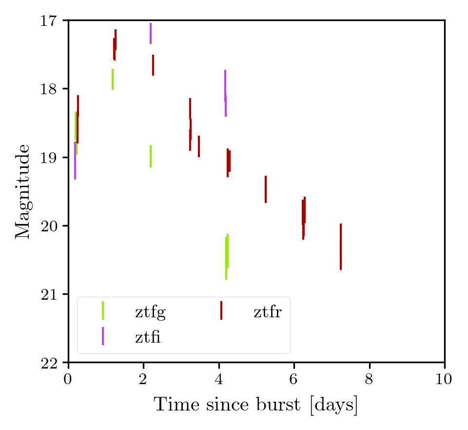
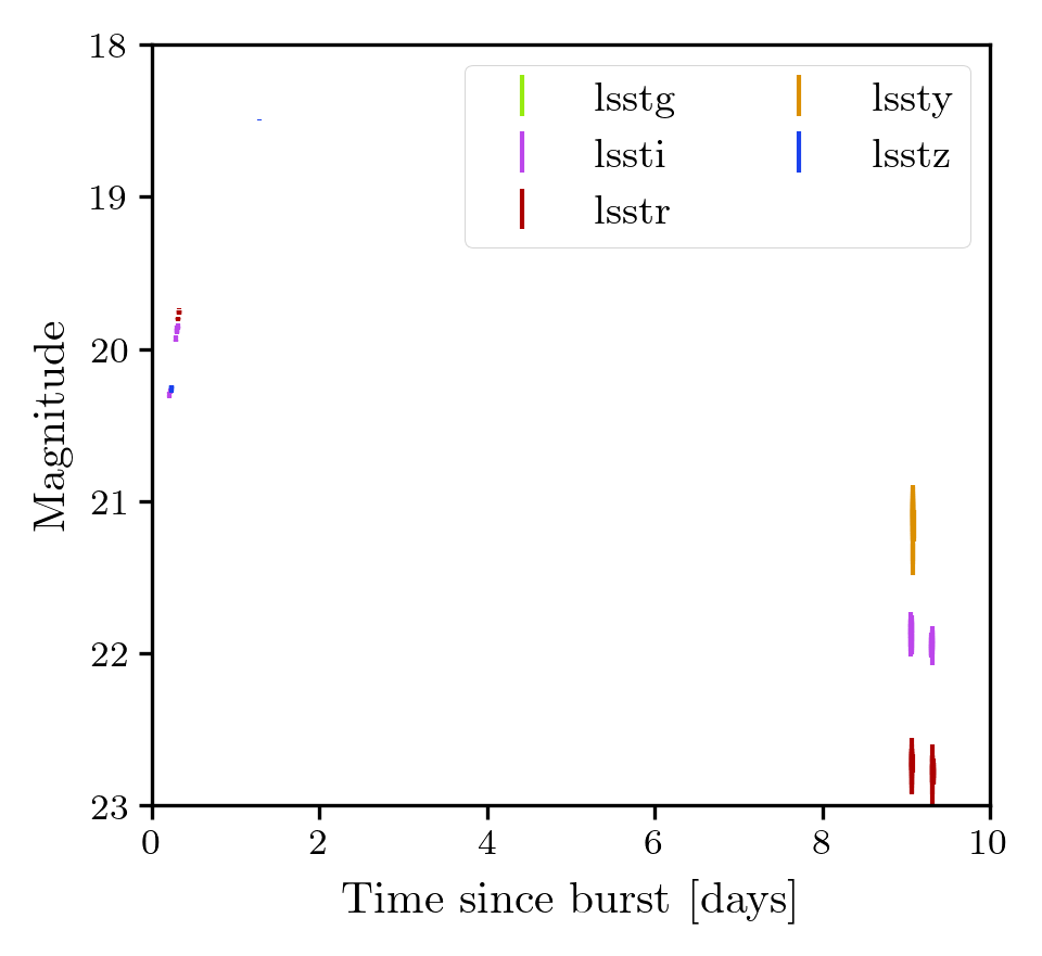
Figure 2: (Left) Simulated kilonova (one component kilonova model) in ZTF and in LSST (Right). We emphasize that aesthetic features such as the colours of the data points, axes limits etc can all be modified by passing in relevant keyword arguments to the plotting methods.

We note that this exact interface can also be used to generate survey lightcurves for the Nancy-Grace Roman Observatory or a user-generated survey and for any model implemented in Redback, and these examples are available at https://github.com/nikhil-sarin/redback. Furthermore Redback also offers the functionality to simulate transients more generically (in a manner more consistent with target of opportunity observations) or simulate a full survey.

5 Multi-messenger analysis

A key advantage of the interface with Bilby is to facilitate multi-messenger gravitational-wave and electromagnetic transient analyses. Here Redback provides the likelihood, model and/or simulated data for the electromagnetic transient and Bilby provides the same for the gravitational-wave data. Both likelihoods communicate together through the use of a joint_likelihood which combined with a full prior, can be used to perform joint multi-messenger analyses.

We demonstrate this feature through the observation of a simulated binary neutron star signal, GW231116, observed in O4 alongside a gamma-ray burst afterglow detected in X-rays. We note that this workflow can be easily extended to also include an optical/radio afterglow and/or a kilonova. Furthermore, the joint likelihood interface can also be used to jointly fit any two data types, e.g., a spectrum and photometry, both of which could be provided by Redback but we leave such examples from this paper for simplicity. This analysis has been performed for GW170817 by multiple groups (e.g., Gianfagna et al., 2023).

We start by setting up the data,

⬇

import bilby

import redback

from astropy.cosmology import Planck18 as cosmo

from redback.transient_models.afterglow_models import tophat

from bilby.core.prior import Uniform

source_redshift = 0.03

source_distance = cosmo.luminosity_distance(source_redshift).value

gw_injection_parameters = dict(mass_1=1.5, mass_2=1.3, chi_1=0.02, chi_2=0.02, luminosity_distance=source_distance,theta_jn=0.43, psi=2.659, phase=1.3, geocent_time=1126259642.413,

ra=1.375, dec=-1.2108, lambda_1=400, lambda_2=450, fiducial=1)

For demonstrative purposes, we assume that the afterglow kinetic energy is some unknown fraction of the total rest mass energy of the binary, alongside the more conventional assumption that the jet is launched along the orbital angular momentum of the binary. These assumptions are not captured by any afterglow model implemented in Redback, so we create a new function, wrapping a simple tophat model already implemented in Redback.

⬇

def get_jet_energy(mass_1, mass_2, fudge):

total_mass = (mass_1 + mass_2)

return total_mass * fudge * 2e33 * 3e10**2

fudge_factor = 0.04

afterglow_energy = get_jet_energy(gw_injection_parameters["mass_1"], gw_injection_parameters["mass_2"],

fudge=fudge_factor)

grb_injection_parameters = dict(fudge=fudge_factor,

theta_jn=gw_injection_parameters["theta_jn"],

redshift=source_redshift, loge0=afterglow_energy,

thc=0.1, logn0=-1, p=2.2, logepse=-1, logepsb=-2, ksin=1,

g0=50, mass_1=gw_injection_parameters["mass_1"],

mass_2=gw_injection_parameters["mass_2"])

def grb_afterglow_model(time, redshift, theta_jn, mass_1, mass_2, fudge, thc, logn0, p,

logepse, logepsb, ksin, g0, **kwargs):

energy = get_jet_energy(mass_1, mass_2, fudge=fudge)

energy = np.log10(energy)

if "loge0" in kwargs.keys():

kwargs.pop("loge0")

return tophat(time=time, redshift=redshift, thv=theta_jn, loge0=energy, thc=thc,

logn0=logn0, p=p, logepse=logepse, logepsb=logepsb,

ksin=ksin, g0=g0, **kwargs)

We can now simulate the electromagnetic data using this model following the method outlined in previous sections or by calling the model directly, and then create a Redback Transient class, alongside an instance of the likelihood. Furthermore, we can set up the gravitational-wave analysis, to reduce the computational cost we use the relative-binning approximation (Zackay et al., 2018). We follow the standard Bilby relative-binning example for this aspect and do not outline the details here. We can also set up the electromagnetic aspect (i.e., the prior and likelihood) via

⬇

em_priors = bilby.core.prior.PriorDict()

em_priors["redshift"] = source_redshift

em_priors["thc"] = Uniform(0.01, 0.2, "thc", latex_label = r"$\theta_{\mathrm{core}}$")

em_priors["logn0"] = Uniform(-4, 2, "logn0", latex_label = r"$\log_{10} n_{\mathrm{ism}}$")

em_priors["p"] = Uniform(2,3, "p", latex_label = r"$p$")

em_priors["fudge"] = Uniform(0.01, 0.1, "fudge", latex_label = r"$f_{\mathrm{fudge}}$")

em_priors["logepse"] = grb_injection_parameters["logepse"]

em_priors["logepsb"] = grb_injection_parameters["logepsb"]

em_priors["ksin"] = grb_injection_parameters["ksin"]

em_priors["g0"] = grb_injection_parameters["g0"]

em_likelihood = redback.likelihoods.GaussianLikelihood(x=sim_afterglow.time,

y=sim_afterglow.flux_density,

function=grb_afterglow_model,

sigma=yerr, kwargs=afterglow_kwargs)

Here, we have first set up a prior on a series of parameters, while fixing some to the injected values to reduce the computational cost of the analysis, and then set up the electromagnetic likelihood, using the Transient object attributes.

Once, the electromagnetic and gravitational-wave is set up (i.e., the individual likelihoods and priors), we can simply set up the joint analysis via,

⬇

joint_likelihood = bilby.core.likelihood.JointLikelihood(gw_likelihood, em_likelihood)

priors_emgw = em_priors.copy()

priors_emgw.update(gw_priors)

Here, the first line sets up a joint likelihood (the product of the two individual likelihoods) and the functional interface for the code to interact correctly. The second line does the same, setting up a prior object, automatically handling parameters that are shared.

Parameter estimation with the joint likelihood can then be performed via the Bilby interface,

⬇

result = bilby.run_sampler(joint_likelihood, priors=priors_emgw, label="emgw", outdir="joint")

In Fig. 3, we show the constraints on various parameters provided by the above analysis, alongside constraints provided under the assumption that they are separate events. The orange lines indicate the true value of the simulation, indicating that the parameters are recovered correctly. In the right-hand panel, we show the fit to the simulated X-ray afterglow plotted via the analysis module. As expected, the primary benefit of including the afterglow is to break the distance-inclination angle degeneracy, clearly improving the estimate of distance and viewing angle for this hypothetical event.

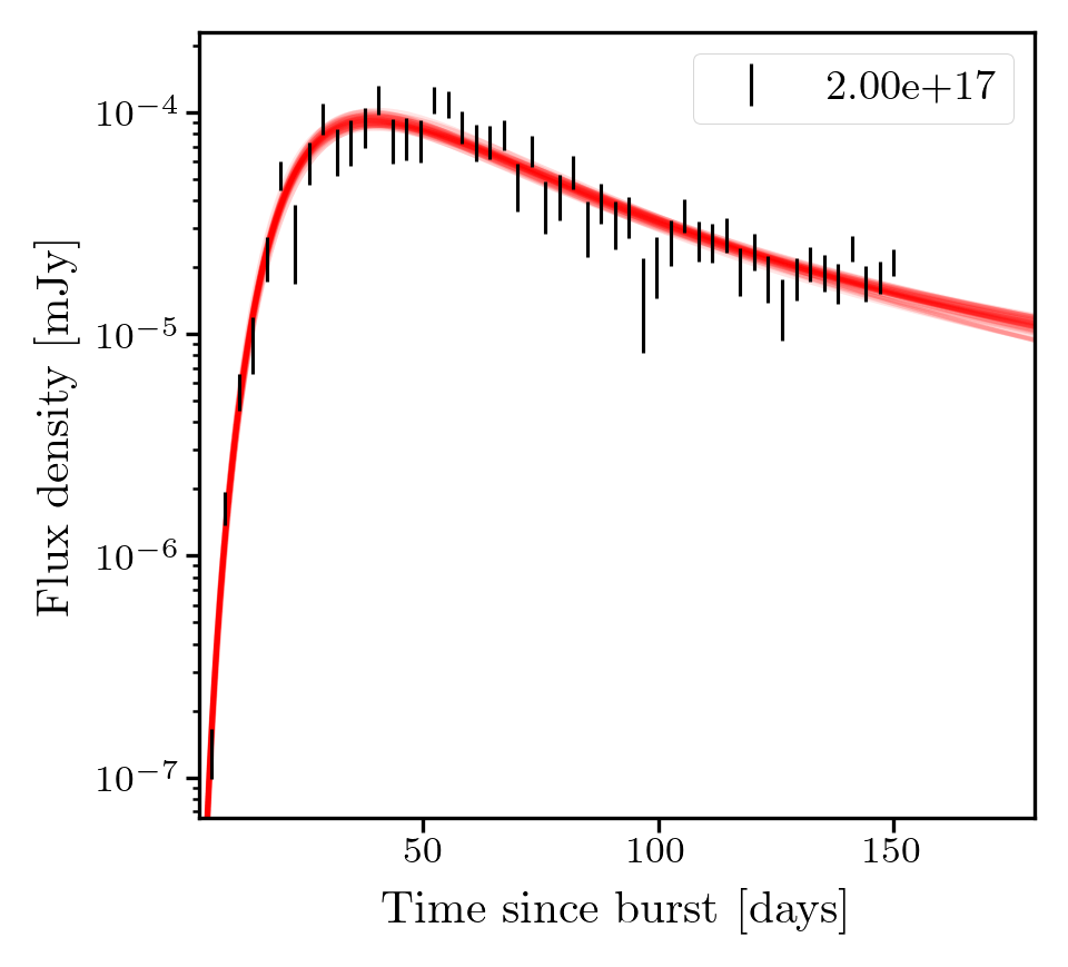
Figure 3: (Left) Corner plot showing the 1-3 $\sigma$ posterior on a subset of parameters with a GW only analysis (blue) and a GW + Afterglow analysis (red), with black lines indicating the input values of the simulation. The right-hand panel shows the lightcurve fit from the joint analysis.

6 Examples

We now go through a series of more general examples that demonstrate how Redback can be used to fit and infer properties of a variety of electromagnetic transients. We note that each of these examples are available as standalone scripts at https://github.com/nikhil-sarin/redback. To aid readability of these examples in this paper, we avoid code snippets that are identical to the snippets described above.

6.1 Broadband afterglow - GRB170817A

We first demonstrate how Redback can be used to fit private or simulated data by fitting the afterglow of GRB170817A (Abbott et al., 2017b; Hallinan et al., 2017; Alexander et al., 2018; Lamb et al., 2019a; Fong et al., 2019). We must first load the data file and create an afterglow Transient object via the method described in Sec. 4.2. After we have created the Transient object and have verified that the data looks correct (by plotting or by inspecting the Transient object), we are ready to fit. We know through many lines of evidence that GRB170817A was observed off-axis (e.g., Fong et al., 2019; Alexander et al., 2018) and the jet was likely structured (e.g., Lamb et al., 2019a; Fong et al., 2019). Furthermore, many previous analyses have already fit the observations of GRB170817A to remarkable success. In particular, we can fit this data with a gaussiancore structured jet model from afterglowpy. As this model is already implemented in Redback, we simply need to specify this model as a string and load the associated prior.

⬇

model = "gaussiancore"

priors = redback.priors.get_priors(model=model)

These lines construct a prior object using the default prior implemented in Redback for the gaussiancore model. To reduce inference wall-time, we can also fix some of the parameters of the model with values consistent as those found by Ryan et al. (2020). This can be done via,

⬇

priors["redshift"] = 1e-2

priors["logn0"] = -2.6

priors["p"] = 2.16

priors["logepse"] = -1.25

priors["logepsb"] = -3.8

priors["ksin"] = 1.

We note that we could have instead set a narrow Gaussian prior around these values instead of fixing these parameters. With these few lines, we are now almost ready for inference. As mentioned in Sec. 3, several Redback models require additional keyword arguments; such as the frequencies at which each data point was was observed and the output format of the model (which must be the same as the data).

⬇

model_kwargs = dict(frequency=afterglow.filtered_frequencies, output_format="flux_density")

Here, we have set up a model dictionary which contains the frequency of the data points (this can be easily extracted from the Transient object via the filtered_frequencies attribute) and set the output format as flux density. We are now ready to fit via,

⬇

result = redback.fit_model(transient=afterglow, model="gaussiancore", sampler="dynesty",

model_kwargs=model_kwargs, prior=priors, nlive=2000, resume=True)

Here we call the Redback fit_model function, which takes as input the afterglow object being fit, the name of the model, sampler, the prior, the model keyword arguments, and any other keyword arguments; and returns the Redback result object. Here we have specified the sampler to be dynesty via a string, but this could be any other sampler implemented in Bilby. We also specify some sampler settings such as the number of live points and the option to resume from a previous run. When finished, this will return the Redback result object, which can be used to create a plot of the corner and a multi-band lightcurve to verify the fit via,

⬇

result.plot_corner(parameters=["thv", "loge0", "thc"])

result.plot_multiband_lightcurve(random_models=100)

Here, in the first line we have also passed a list of the parameters we wish to show and in the second asked for 100 randomly sampled lightcurves from the posterior to be plotted. Note that several other arguments can be passed into these functions to change aesthetics or the type of information displayed. These two plots are shown in Fig. 4.

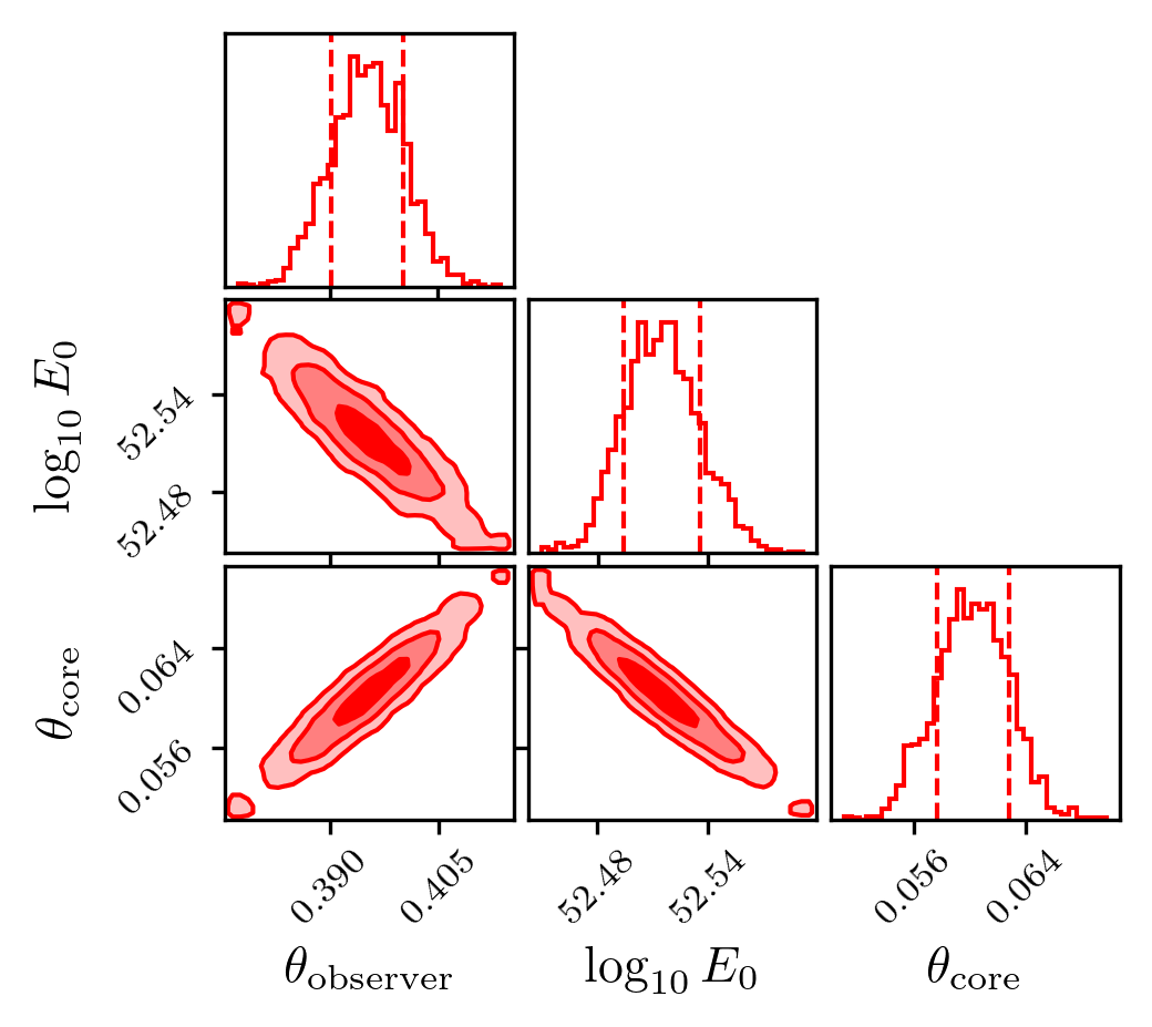
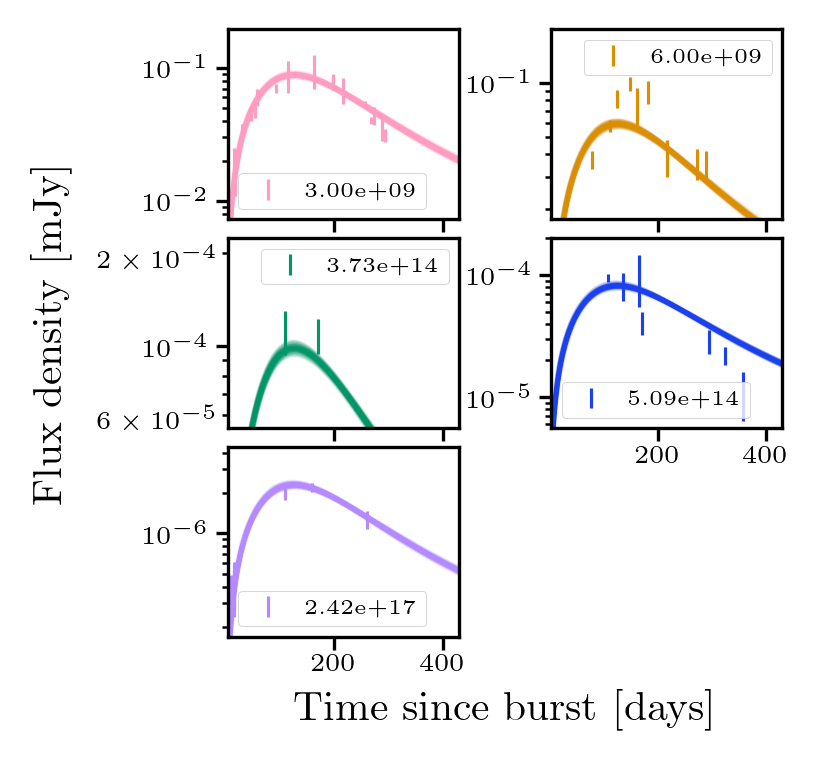
Figure 4: (Left) Posterior on the observers viewing angle, the isotropic equivalent energy of the afterglow and the opening angle of the relativistic jet from fitting the afterglow of GRB170817A with the different shading indicating the $1-3\sigma$ credible intervals. (Right) Data of the afterglow of GRB170817A at multiple frequencies along with the lightcurves from a 100 random draws from the posterior.

6.2 Kilonova - AT2017gfo

We now demonstrate how Redback can be used to fit a kilonova, in particular the kilonova that accompanied GW170817, AT2017gfo (Abbott et al., 2017b; Villar et al., 2017). For simplicity, we will fit a one_component_kilonova_model implemented within Redback to observations of AT2017gfo (Villar et al., 2017). Such a model is known to not provide a great fit to the data so this is merely a demonstration of Redback functionality. As mentioned in Sec. 3, significantly more complex kilonovae models are available in Redback which have been previously shown to well explain the observations (e.g., Villar et al., 2017; Bulla, 2019; Nicholl et al., 2021).

The data of AT2017gfo is available at OAC (Guillochon et al., 2017), which can be obtained via the code shown in Sec. 4.1.

⬇

data = redback.get_data.get_kilonova_data_from_open_transient_catalog_data(transient="at2017gfo")

The above code calls the get_data module to obtain the data for AT2017gfo from the OAC. As mentioned above, this will return a pandas data frame while also saving the data to disk. Users can manipulate the data as they would any other pandas object. However, for our purpose it is more useful to use this data to create an kilonova object. This is done via

⬇

kilonova = redback.kilonova.Kilonova.from_open_access_catalogue(

name="at2017gfo", data_mode="flux_density", active_bands=np.array(["g", "i"]))

Here we have created a kilonova Transient object, specifying the data mode to be flux density. We have also set the ‘g’ and ‘i’ bands as active, which will disable all other bands and only fit the active bands. This can be done to both reduce the computational time of inference but also for cases when the data or model are unreliable for specific filters. To ensure the data is correctly processed, we can plot the data via

⬇

kilonova.plot_data(show=True, save=False, plot_others=False, band_colors={"g":"green", "i":"indigo"}, xlim_high=10)

fig, axes = plt.subplots(3, 2, sharex=True, sharey=True, figsize=(12, 8))

kilonova.plot_multiband(figure=fig, axes=axes, filters=["g", "r", "i", "z", "y", "J"])

Here the first line will plot all the data onto one figure, where we have also passed additional arguments such a dictionary of the colors for each band, whether to plot the inactive bands, to not save and to show the plot and the upper limit on the x axis. Note that Redback returns the matplotlib axes so several other plotting related things can be changed by the user directly or by passing in an additional keyword argument. The second line, will make a plot with one band per axes and we have also specified the specific filters we wish to display. Note that this functionality allows us to show data for a filter or fits for a filter even if that filter was set as inactive. Both figures are shown in Figure 5.

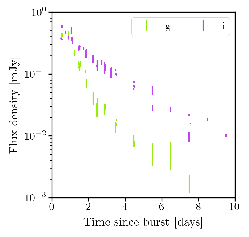
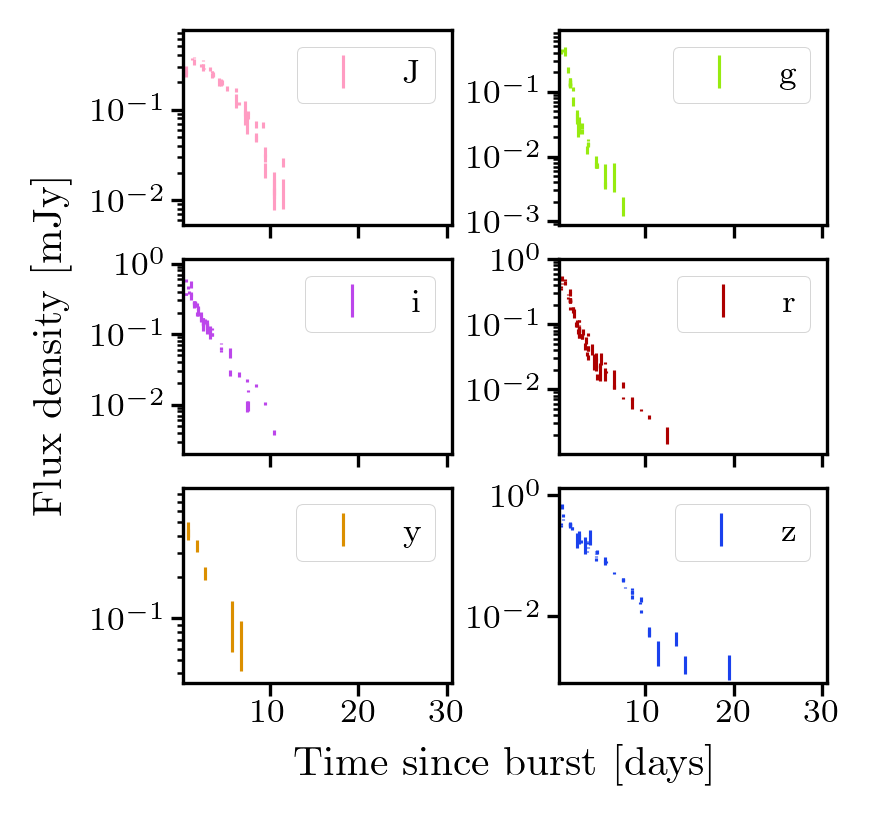
Figure 5: (Left) Data of AT2017gfo plotted through the plot_data method. (Right) Data of the AT2017gfo plotted through the plot_multiband method.

With the Transient object created and data verified through a plot, we are now ready to fit. As mentioned above, we will fit with the a one component kilonova model. However, we will now also demonstrate how a user can fit the data with a different likelihood and sampler. We skip steps to load a prior and set up model keyword argument dictionary as they are identical to the afterglow example above.

⬇

prior["sigma"] = Uniform(0.01, 0.0001, name="sigma", latex_label="$\sigma$")

function = all_models_dict[model]

sampler = "nestle"

Here, we first define a new prior on a parameter sigma, which is an additional parameter to be fit for, then use a convenience dictionary to get the Redback function for a one component kilonova model and specify the sampler to be used in inference as the nestle sampler. We note that sigma is the uncertainty in the typical Gaussian likelihood (i.e., $\sigma$), and if a user provides a prior but uses the standard (default) likelihood, this will overwrite the specific measured errors for a constant $\sigma$ that is estimated by sampling. However, here, we wish to demonstrate the use of a custom likelihood (either something provided by the user or a different likelihood already implemented in Redback), we can do this using the processed attributes from the Transient object via,

⬇

likelihood = redback.likelihoods.GaussianLikelihoodQuadratureNoise(x=kilonova.x[kilonova.filtered_indices], y=kilonova.y[kilonova.filtered_indices], sigma_i=kilonova.y_err[kilonova.filtered_indices], function=function)

Here, we use a Gaussian Likelihood with an additional noise source, $\sigma$ added in quadrature (that is fitted for) to the measured y errors. This likelihood is already implemented in Redback but a user could easily replace this likelihood with their own class. Then, users can use this likelihood in the fit via,

⬇

result = redback.fit_model(transient=kilonova, model=model, likelihood=likelihood, sampler=sampler,

model_kwargs=model_kwargs, prior=priors)

With this simple change we can fundamentally change what we believe to be the data generation process and ensured that advanced users can easily change the likelihood and settings of the sampler, without ever digging into the Redback source code.

6.3 Supernova - SN1998bw

Redback can also be used to fit supernovae. Here we fit the arnett model (Arnett, 1980, 1982) implemented within Redback to observations of SN1998bw (Galama et al., 1998). We can acquire the data for SN1998bw through the OAC and API shown above and create a supernova object.

After ensuring that the data is obtained correctly we can set up the fit in a few lines of code. As the arnett model is already implemented in Redback we can simply load up the default prior for this model via,

⬇

priors = redback.priors.get_priors(model="arnett")

priors["redshift"] = 0.0085

Here we have also fixed the redshift to the known redshift of SN1998bw. We can now set up the fit in another two lines of code.

⬇

model_kwargs = dict(frequency=supernova.filtered_frequencies, output_format="flux_density")

result = redback.fit_model(transient=supernova, model="arnett", sampler="dynesty", model_kwargs=model_kwargs,

prior=priors, nlive=500, clean=True, npool=4)

Here, we have also specified npool=4 which will set up the dynesty sampler with multiprocessing over 4 cores to reduce the wall-time of the analysis. We have also set the option clean to True, which ensures that Redback will restart this analysis from scratch and not resume from a previous analysis.

As with all other analysis, the fit returns a Redback result object, which we can use to obtain posteriors on various parameters, or for plotting. For example, we can plot the lightcurve with the fit shown as a $68\%$ credible interval (shown in Fig. 6) via,

⬇

ax = result.plot_lightcurve(uncertainty_mode="credible_intervals", plot_others=False, show=False,

credible_interval_level=0.68)

ax.set_xscale("log")

ax.set_xlim(10, 300)

plt.show()

Here we have also returned the matplotlib axes and used this to modify the xscale and xlimits of the plot. The fit demonstrates the large uncertainty at early times where there are no observations in these bands.

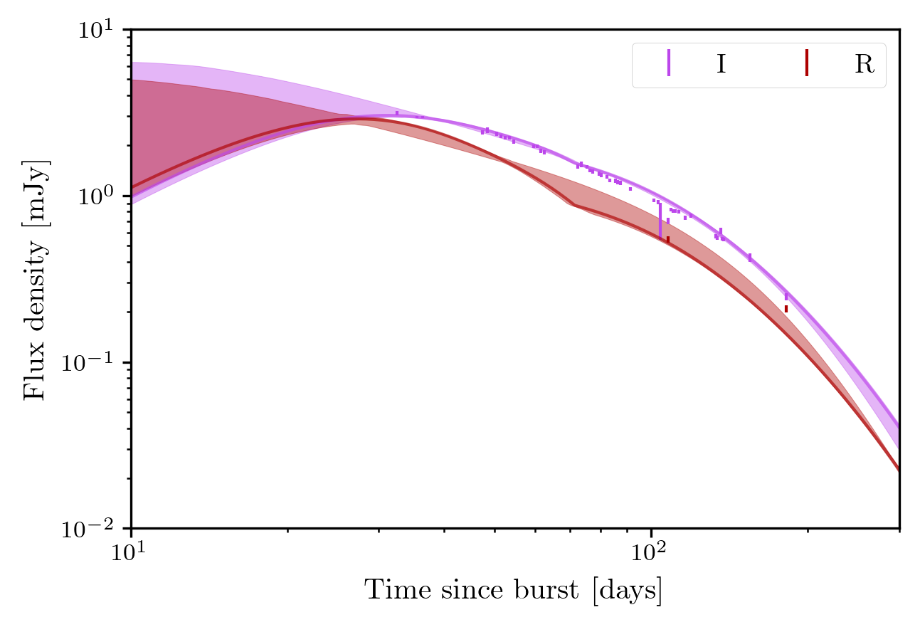
Figure 6: R and I band observations of SN1998bw alongside the $68\%$ credible interval from our fit.

6.4 Tidal disruption events - PS18kh

Here, we fit the tde_analytical model implemented within Redback to multiband observations of, tidal disruption event, PS18kh (Holoien et al., 2019). We acquire the data from OAC and create a tde Transient object. We set only a subset of bands as active via,

⬇

tidal_disruption_event.active_bands = ["V", "g", "r"]

The rest of the code to fit is exactly like the afterglow example above. We can visualise our fit and make the predicted lightcurve (shown in Fig. 7) for multiple filters, including a filter that we did not fit, e.g., the u-band, via

⬇

result.plot_multiband_lightcurve(random_models=100, filters=["V", "g", "r", "u"])

This is a useful verification exercise to understand which filters are driving the fit and whether the fits without a certain band are consistent with those observations.

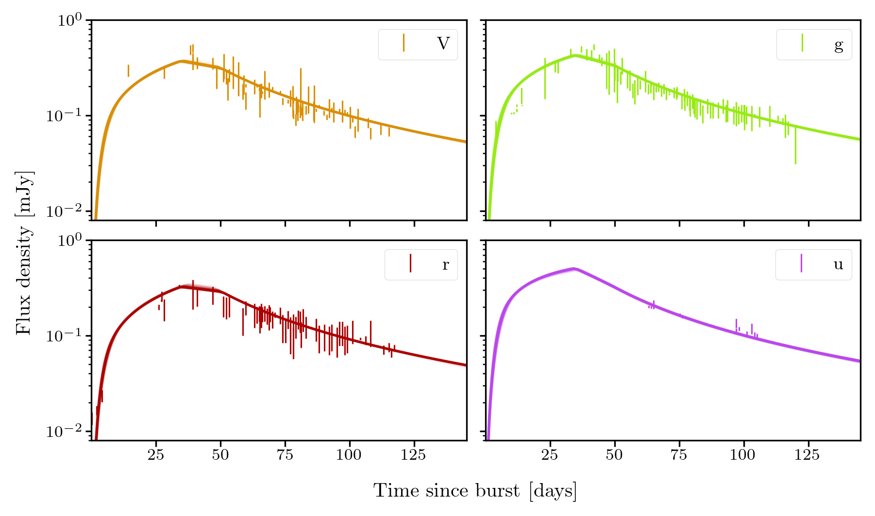
Figure 7: Multiband light curve of PS18bh along with the fitted lightcurve from a 100 random realisations randomly drawn from the prior.

6.5 X-ray afterglow of GRB070809 - millisecond magnetars

We now use Redback on an integrated flux or luminosity data by fitting the X-ray afterglows of a gamma-ray burst, by fitting the evolving_magnetar model (Şaşmaz Muş et al., 2019) to Swift observations of GRB070809, specifically the integrated flux obtained from Swift-XRT.

We acquire the BAT and XRT data of GRB070809 from Swift via the get_data module

⬇

redback.get_data.get_bat_xrt_afterglow_data_from_swift(grb="070809", data_mode="flux")

We construct an afterglow class instance via

⬇

afterglow = redback.afterglow.SGRB.from_swift_grb(name="070809", data_mode="flux",

truncate=True, truncate_method="prompt_time_error")

afterglow.analytical_flux_to_luminosity()

ax = afterglow.plot_data()

Here, we have specified to load the flux data for GRB070809 from Swift. This data typically also includes BAT data from the prompt phase which we do not wish to fit here. We truncate this data using the prompt_time_error method.

The evolving_magnetar model works on luminosity data. We could have provided this data when creating the afterglow object but we also provide two convenience functions to generate this data, an analytical method which uses the GRBs photon index and a numerical method from Sherpa which uses the spectrum. All details necessary for either method are obtained internally by Redback from the Swift Data Centre. Here, we use the analytical method to convert the integrated flux data to a luminosity.

⬇

afterglow.analytical_flux_to_luminosity()

Note, that this will automatically change the afterglow objects data mode to luminosity. Beyond this point, the fitting workflow is identical to fitting any other transient i.e.,

⬇

priors = redback.priors.get_priors(model="evolving_magnetar")

result = redback.fit_model(model="evolving_magnetar", sampler="dynesty", nlive=200, transient=afterglow,

prior=priors, sample="rslice", resume=True)

The above code first constructs a prior object, using the default prior implemented in Redback for the evolving_magnetar model. This is followed by code calling fit_model. Note that here we do not need a dictionary for the model keywords as this model does not require any. We are again returned the Redback result object which can be used to plot a corner plot, the lightcurve or obtain any other diagnostic about the inference/posterior. For these data modes however, it can be especially informative to show a plot of the lightcurve with the residuals. This can be obtained using plot_residual method of the result object. This generates Fig. 8, where the top panel shows the data in black with maximum likelihood and random draws in blue and red respectively with the bottom panel showing the residual between the data and the maximum likelihood model.

⬇

result.plot_residual()

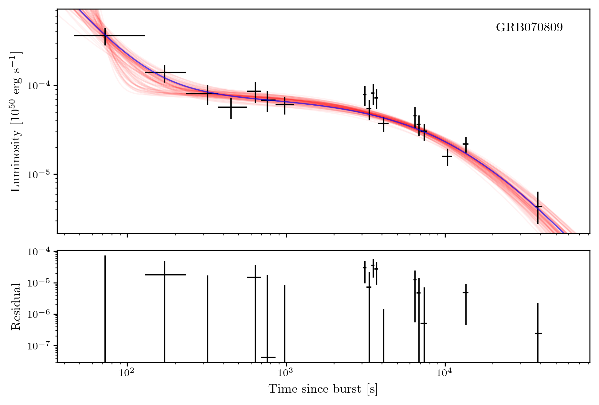
Figure 8: Residual plot obtained using plot_residual method of the result object. Here the top panel shows the data in black with maximum likelihood and 100 randomly drawn lightcurves in blue and red respectively with the bottom panel showing the residual between the data and the maximum likelihood model.

6.6 Phase and Attenuation - SN2018ibb

In previous examples, we have ignored two important aspects of fitting transients; 1) We often do not know when the explosion occured and 2) there is attenuation in the form of dust extinction from the host galaxy.

In this example, we show how to fit data while measuring the unknown explosion time and including extinction. We will also demonstrate how to fit in magnitudes and adding a new filter to Redback and SNCosmo. We will do this by fitting a supernova, in particular, the UV-to-NIR light curve of the superluminous supernova SN 2018ibb (Schulze et al., 2023).

As previous examples, we can load the private data for SN 2018ibb and create a Supernova Transient object via

First, we read in the private data.

⬇

import pandas as pd

data = pd.read_csv("SN2018ibb_photcat_Redback.ascii", sep="")

sn=redback.transient.Supernova(name = "SN2018ibb",

data_mode = "magnitude", time_mjd = data["MJD"].values,

magnitude = data["MAG"].values, magnitude_err = data["MAG_ERR"].values, bands = data["band"].values,

use_phase_model = True)

In contrast to the previous examples, we fit the data in magnitude space. Furthermore, we set use_phase_model = True because we do not know the explosion date. We also specify time values in MJD instead of days since explosion. When fitting a model to such data, a user must then add a prior on the explosion time which will then be sampled over. We note that use_phase_model = True, will also change plotting labels to account for the change.

Before we can fit the magnitude data of SN 2018ibb, we must first ensure that all filters of the observations are available in Redback. We note that this is only a concern when fitting photometry in magnitudes or flux as this requires the full transmission curve of every filter rather than a reference wavelength. Some of the observations of SN 2018ibb were performed with the GROND camera mounted at the 2.2 m MPG telescope. The GROND filters (in our example grond::i and grond::z) are not part of SNCosmo distribution that is used internally within Redback for filter definitions. After retrieving the filters, for instance, from the Spanish Virtual Observatory (Rodrigo et al., 2012), we add them to SNCosmo and by extension Redback, via

⬇

from astropy.io import ascii

import astropy.units as u

import sncosmo

filter_files = [

"/PATH/WHERE/YOU/STORED/FILTER_CURVES/GROND_I.dat",

"/PATH/WHERE/YOU/STORED/FILTER_CURVES/GROND_Z.dat",

]

filter_names = ["grond::i", "grond::z"]

for f, fname in zip(filter_names, filter_files):

_data = ascii.read(fname)

band = sncosmo.Bandpass(_data["col1"], _data["col2"], name=f, wave_unit=u.angstrom)

sncosmo.register(band, f, force=True)

We can set up the rest of the inference workflow, first set up the model and the prior via

⬇

model = "t0_supernova_extinction"

base_model = "arnett"

priors = redback.priors.get_priors(model=model)

priors.update(redback.priors.get_priors(model=base_model))

Here we choose the t0_supernova_extinction model, which has the explosion time and magnitude of extinction as a free parameter. This model itself does not contain any physics and must be specified an additional physical model. For simplicity, we use the physical arnett model as the base model. The last two lines of code just set up the prior object to include the parameters of both models.

We must now also set priors on the explosion time, the extinction magnitude and update the prior on the ejecta mass as SN 2018ibb requires an extraordinary amount of ejecta (Schulze et al., 2023).

⬇

from bilby.core.prior import Uniform

# Allow the explosion date to be up to 200 days before the first detection

priors["t0"] = Uniform(minimum = data["MJD"].values.min()-200, maximum = data["MJD"].values.min()-1, name = "t0", latex_label = r"$t_{\rm expl.}$")

priors["mej"] = Uniform(minimum = 1, maximum = 260, name = "mej", latex_label = r"$M_{\rm{ej}}~(M_{\odot})$")

# Extinction

priors["av"] = Uniform(minimum = 0, maximum = 1, name = "av",latex_label = r"$A_V$ (mag)")

With the model specified and prior set up, we can now fit via,

⬇

model_kwargs = dict(bands = sn.filtered_sncosmo_bands, base_model = base_model, output_format = "magnitude")

result = redback.fit_model(transient = sn, model = model, model_kwargs = model_kwargs,

prior = priors, plot = True)

We note that as we are fitting with a base model and in magnitudes, there are some minor differences to the model_kwargs, namely that we must now specify a list of bands for the data points instead of frequency and must specify the base model. In the fit_model argument, we have also set plot=True, which will automatically generate the fitted lightcurve after inference finishes. In Fig 9, we show the lightcurve fit generated with the above code and the result.plot_multiband_lightcurve().

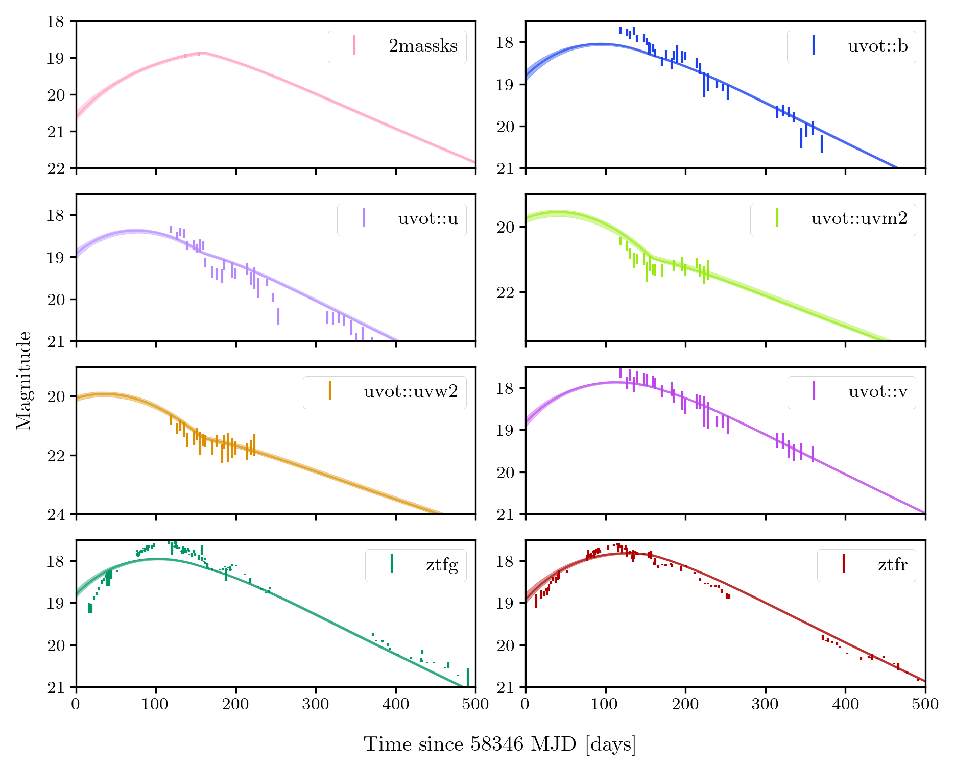
Figure 9: Multiband light curve of SN2018ibb along with the $68\%$ credible interval lightcurve fit from the posterior.

7 Future development

As we continue to drive progress in transient astronomy, we develop newer and better models for transients and make improvements to how we treat the data. This paper marks version 1.0 release but Redback will be further developed to keep pace with the developments in modelling and treatment of data.

One of the primary aspects that will be improved are the models implemented in Redback. In particular, we are currently implementing models for interacting supernovae and fast-blue optical transients, from semi-analytical models of shocks produced by interacting shells (Margalit, 2022), to surrogates of radiative transfer simulations (Khatami & Kasen, 2023). We are also improving some of our models of afterglows for better treatment of reverse shocks and to make them more computationally efficient. We will soon implement model for $r$-process nucleosynthesis from collapsars (Barnes & Metzger, 2022; Anand et al., 2023). On longer timescales we will implement models with better spectral modelling, enabling joint fitting of the spectrum and photometry.

Alongside improvements and addition of models, we will further develop Redback for more practical purposes, for example, providing a generic interface in redback_surrogate to allow users to make their own surrogate from a grid of simulations and newer likelihoods that better describe the data generation process. We will also be further developing the simulation module to improve our treatment of focal plane geometry. On longer timescales, we will add some GPU implementations of models to enable rapid inference and an API to download and process data from the Fermi catalog (e.g., von Kienlin et al., 2020).

8 Conclusion

Realising the rich promise of the large transient data expected from new observing facilities such as the Vera Rubin Observatory and ULTRASAT (Shvartzvald et al., 2023) requires us to confront such data with models describing the different transient phenomena. This requires fast, reliable, open source code that is both accessible to newcomers to the field and modular such that it can be adapted to be the powerhouse required by experts. Here, we have described Redback, a Bayesian inference software package for end-to-end for parameter estimation and interpretation of electromagnetic transients.

In this paper, we have described the overall design of Redback and demonstrated the functionality and usability of the software. Redback is object orientated, enabling users to input their own model, priors, data without needing to edit the source code. The interface to Bilby also provides access to a large variety of samplers enabling validation across samplers and easy multi-messenger analysis for joint events such as GW170817 (e.g., Radice et al., 2018; Coughlin et al., 2019; Gianfagna et al., 2023). Redback is an engine for simulating realistic transients and inferring their properties enabling end-to-end analysis and validation of inference workflows. Furthermore, one can also use this software to understand how to optimize survey strategies/design or understand the selection function of different telescopes/surveys. Redback is also fully Bayesian, enabling the vast advantages of this statistical paradigm such as model selection, importance sampling, and Bayesian hierarchical modelling. As discussed in Sec. 7, we will continue to further develop Redback, including the addition of newer models and additional functionality. Redback has already been used in previous publications such as inference on tidal disruption events (Sarin & Metzger, 2023), analysis of SN 2018ibb (Schulze et al., 2023), magnetar-driven kilonovae and supernovae (Sarin et al., 2022b; Omand & Sarin, 2023), GRB afterglows (Sarin et al., 2021, 2022a), and to infer joint GRB and kilonovae observations (Levan et al., 2023), demonstrating the flexibility of the software and ease of use. A more comprehensive comparison of results for different transient catalogs is underway alongside interpretation for other transients.

9 Acknowledgments

We thank Duncan Galloway, Phil Macias, Dougal Dobie, Karelle Siellez, Fiona Panther, Jacob Wise, Ariel Goobar, and Miti Patel for helpful comments on the software or manuscript. We are grateful to several members of the astronomical community for releasing their transient models as modular open-source software, many of these models form part of the available models in Redback. We hope the practice of releasing open-source software gathers more pace in transient astronomy. We also acknowledge the work done by numerous people to maintain public catalogs such as Swift Data Centre, OAC, Fink, and Lasair.

N. Sarin is supported by a Nordita Fellowship. Nordita is supported in part by NordForsk. S. Schulze and A. Sagués-Carracedo acknowledge support from the G.R.E.A.T. research environment, funded by Vetenskapsrådet, the Swedish Research Council, project number 2016-06012.

A part of this work used computing facilities provided by the OzSTAR national facility at Swinburne University of Technology. The OzSTAR program receives funding in part from the Astronomy National Collaborative Research Infrastructure Strategy (NCRIS) allocation provided by the Australian Government.

The Redback package makes use of the standard scientific python stack (Jones et al., 2001; Harris et al., 2020; McKinney, 2010), matplotlib (Hunter, 2007), and corner (Foreman-Mackey, 2016), for the generation of figures, and astropy (Robitaille et al., 2013; Price-Whelan et al., 2018; Astropy Collaboration et al., 2022) for common astrophysics-specific operations. Redback makes use of Bilby (Ashton et al., 2019; Romero-Shaw et al., 2020) to provide an interface to different sampling algorithms and for evaluating prior distributions. Redback uses SNCosmo (Barbary et al., 2022) for filter definitions and calculations of magnitude from SEDs, extinction (Barbary, 2016) for extinction corrections. And requests and selenium for downloading data from catalogs.

10 Data Availability

The software package along with example scripts for all analysis demonstrated in this manuscript alongside a plotting notebook to generate all the plots as well as other examples are available at https://github.com/nikhil-sarin/redback. The specific result objects for each of the analyses presented here are available at https://doi.org/10.5281/zenodo.8273145. Redback is available on pypi. This paper uses v1.0 release of Redback with documentation at https://redback.readthedocs.io/en/latest/. The data for all transients is available at the Open Access Catalog (Guillochon et al., 2017) gathered through the Redback get_data module or hosted at https://github.com/nikhil-sarin/redback.

References

- Abbott et al. (2017a) Abbott B. P., Abbott R., Abbott T. D., Acernese F., et al. 2017a, Phys. Rev. Lett., 119, 161101
- Abbott et al. (2017b) Abbott B. P., et al., 2017b, Astrophys. J., 848, L12
- Alexander et al. (2018) Alexander K. D., Margutti R., Blanchard P. K., Fong W., et al. 2018, ApJ, 863, L18
- Anand et al. (2023) Anand S., Barnes J., Yang S., Kasliwal M. M., et al. 2023, arXiv e-prints, p. arXiv:2302.09226
- Arcavi et al. (2016) Arcavi I., Wolf W. M., Howell D. A., Bildsten L., et al. 2016, ApJ, 819, 35
- Arcavi et al. (2017) Arcavi I., Hosseinzadeh G., Howell D. A., McCully C., et al. 2017, Nature, 551, 64
- Arnett (1980) Arnett W. D., 1980, ApJ, 237, 541
- Arnett (1982) Arnett W. D., 1982, ApJ, 253, 785
- Ashton et al. (2019) Ashton G., Hübner M., Lasky P. D., Talbot C., et al. 2019, ApJS, 241, 27
- Astropy Collaboration et al. (2022) Astropy Collaboration Price-Whelan A. M., Lim P. L., Earl N., et al. 2022, ApJ, 935, 167
- Banerjee et al. (2020) Banerjee S., Tanaka M., Kawaguchi K., Kato D., et al. 2020, ApJ, 901, 29
- Barbary (2016) Barbary K., 2016, Extinction V0.3.0, Zenodo, doi:10.5281/zenodo.804967
- Barbary et al. (2022) Barbary K., Bailey S., Barentsen G., Barclay T., et al. 2022, SNCosmo, Zenodo, doi:10.5281/zenodo.6363879
- Barnes & Metzger (2022) Barnes J., Metzger B. D., 2022, ApJ, 939, L29
- Bellm et al. (2019) Bellm E. C., Kulkarni S. R., Graham M. J., Dekany R., et al. 2019, PASP, 131, 018002
- Buchner et al. (2014) Buchner J., et al., 2014, Astron. Astrophys., 564, A125
- Bulla (2019) Bulla M., 2019, MNRAS, 489, 5037
- Cano et al. (2017) Cano Z., Wang S.-Q., Dai Z.-G., Wu X.-F., 2017, Advances in Astronomy, 2017, 8929054
- Chatzopoulos et al. (2013) Chatzopoulos E., Wheeler J. C., Vinko J., Horvath Z. L., et al. 2013, ApJ, 773, 76
- Chirenti et al. (2023) Chirenti C., Dichiara S., Lien A., Miller M. C., et al. 2023, Nature, 613, 253
- Cook et al. (2006) Cook S. R., Gelman A., Rubin D. B., 2006, Journal of Computational and Graphical Statistics, 15, 675
- Coughlin et al. (2019) Coughlin M. W., Dietrich T., Margalit B., Metzger B. D., 2019, MNRAS, 489, L91
- Coulter et al. (2017) Coulter D. A., Foley R. J., Kilpatrick C. D., Drout M. R., et al. 2017, Science, 358, 1556
- Cowperthwaite et al. (2017) Cowperthwaite P. S., Berger E., Villar V. A., Metzger B. D., et al. 2017, ApJ, 848, L17
- Dall’Osso et al. (2011) Dall’Osso S., Stratta G., Guetta D., Covino S., et al. 2011, A&A, 526, A121
- Dorsman et al. (2023) Dorsman B., Raaijmakers G., Cenko S. B., Nissanke S., et al. 2023, ApJ, 944, 126
- Drout et al. (2014) Drout M. R., Chornock R., Soderberg A. M., Sanders N. E., et al. 2014, ApJ, 794, 23
- Evans et al. (2010) Evans P. A., Willingale R., Osborne J. P., O’Brien P. T., et al. 2010, A&A, 519, A102
- Fishman et al. (1994) Fishman G. J., Meegan C. A., Wilson R. B., Brock M. N., et al. 1994, ApJS, 92, 229
- Fong et al. (2019) Fong W., Blanchard P. K., Alexander K. D., Strader J., et al. 2019, ApJ, 883, L1
- Foreman-Mackey (2015) Foreman-Mackey D., 2015, George: Gaussian Process regression, Astrophysics Source Code Library, record ascl:1511.015 (ascl:1511.015)
- Foreman-Mackey (2016) Foreman-Mackey D., 2016, The Journal of Open Source Software, 24
- Foreman-Mackey et al. (2017) Foreman-Mackey D., Agol E., Ambikasaran S., Angus R., 2017, celerite: Scalable 1D Gaussian Processes in C++, Python, and Julia, Astrophysics Source Code Library, record ascl:1709.008 (ascl:1709.008)
- Galama et al. (1998) Galama T. J., Vreeswijk P. M., van Paradijs J., Kouveliotou C., et al. 1998, Nature, 395, 670
- Gehrels et al. (2004) Gehrels N., Chincarini G., Giommi P., Mason K. O., et al. 2004, ApJ, 611, 1005
- Gianfagna et al. (2023) Gianfagna G., Piro L., Pannarale F., Van Eerten H., et al. 2023, MNRAS, 523, 4771
- Gottlieb et al. (2018) Gottlieb O., Nakar E., Piran T., 2018, MNRAS, 473, 576
- Greiner et al. (2015) Greiner J., et al., 2015, Nature, 523, 189
- Guillochon & Ramirez-Ruiz (2013) Guillochon J., Ramirez-Ruiz E., 2013, ApJ, 767, 25
- Guillochon et al. (2017) Guillochon J., Parrent J., Kelley L. Z., Margutti R., 2017, ApJ, 835, 64
- Guillochon et al. (2018) Guillochon J., Nicholl M., Villar V. A., et al. 2018, ApJS, 236, 6
- Hallinan et al. (2017) Hallinan G., Corsi A., Mooley K. P., Hotokezaka K., et al. 2017, Science, 358, 1579
- Harris et al. (2020) Harris C. R., et al., 2020, Nature, 585, 357
- Hills (1975) Hills J. G., 1975, Nature, 254, 295
- Hogg et al. (2010) Hogg D. W., Bovy J., Lang D., 2010, arXiv e-prints, p. arXiv:1008.4686
- Holoien et al. (2019) Holoien T. W. S., Huber M. E., Shappee B. J., et al. 2019, ApJ, 880, 120
- Hotokezaka & Nakar (2020) Hotokezaka K., Nakar E., 2020, ApJ, 891, 152
- Hübner et al. (2022) Hübner M., Huppenkothen D., Lasky P. D., Inglis A. R., et al. 2022, ApJ, 936, 17
- Hunter (2007) Hunter J. D., 2007, Computing In Science & Engineering, 9, 90
- Ivezić et al. (2019) Ivezić Ž., Kahn S. M., Tyson J. A., Abel B., et al. 2019, ApJ, 873, 111
- Jones et al. (2001) Jones E., et al., 2001, SciPy: Open source scientific tools for Python, http://www.scipy.org/
- Kasen et al. (2017) Kasen D., Metzger B., Barnes J., Quataert E., et al. 2017, Nature, 551, 80
- Kathirgamaraju et al. (2019) Kathirgamaraju A., Giannios D., Beniamini P., 2019, MNRAS, 487, 3914
- Kessler et al. (2009) Kessler R., Bernstein J. P., Cinabro D., Dilday B., et al. 2009, PASP, 121, 1028
- Khatami & Kasen (2023) Khatami D., Kasen D., 2023, arXiv e-prints, p. arXiv:2304.03360
- Klion et al. (2021) Klion H., Duffell P. C., Kasen D., Quataert E., 2021, MNRAS, 502, 865
- Korobkin et al. (2012) Korobkin O., Rosswog S., Arcones A., Winteler C., 2012, MNRAS, 426, 1940
- Korobkin et al. (2021) Korobkin O., Wollaeger R. T., Fryer C. L., Hungerford A. L., et al. 2021, ApJ, 910, 116
- Lamb et al. (2019a) Lamb G. P., Lyman J. D., Levan A. J., Tanvir N. R., et al. 2019a, ApJ, 870, L15
- Lamb et al. (2019b) Lamb G. P., Tanvir N. R., Levan A. J., de Ugarte Postigo A., et al. 2019b, ApJ, 883, 48
- Lamb et al. (2020) Lamb G. P., Levan A. J., Tanvir N. R., 2020, ApJ, 899, 105
- Lamb et al. (2021) Lamb G. P., Kann D. A., Fernández J. J., Mandel I., et al. 2021, MNRAS, 506, 4163
- Lasky et al. (2017) Lasky P. D., Leris C., Rowlinson A., Glampedakis K., 2017, ApJ, 843, L1
- Levan et al. (2023) Levan A., Gompertz B. P., Salafia O. S., Bulla M., et al. 2023, arXiv e-prints, p. arXiv:2307.02098
- Lukošiute et al. (2022) Lukošiute K., Raaijmakers G., Doctor Z., Soares-Santos M., et al. 2022, MNRAS, 516, 1137
- Mackay (2003) Mackay D. J. C., 2003, Information Theory, Inference and Learning Algorithms
- Margalit (2022) Margalit B., 2022, ApJ, 933, 238
- Margalit & Quataert (2021) Margalit B., Quataert E., 2021, ApJ, 923, L14
- Margalit et al. (2022) Margalit B., Quataert E., Ho A. Y. Q., 2022, ApJ, 928, 122
- McKinney (2010) McKinney W., 2010, Proceedings of the 9th Python in Science Conference, 51-56
- Metzger (2019) Metzger B. D., 2019, Living Reviews in Relativity, 23, 1
- Metzger (2022) Metzger B. D., 2022, ApJ, 937, L12
- Metzger & Piro (2014) Metzger B. D., Piro A. L., 2014, MNRAS, 439, 3916
- Metzger et al. (2010) Metzger B. D., Martínez-Pinedo G., Darbha S., Quataert E., et al. 2010, MNRAS, 406, 2650
- Mockler et al. (2019) Mockler B., Guillochon J., Ramirez-Ruiz E., 2019, ApJ, 872, 151
- Möller et al. (2021) Möller A., Peloton J., Ishida E. E. O., Arnault C., et al. 2021, MNRAS, 501, 3272
- Nakar & Piran (2011) Nakar E., Piran T., 2011, Nature, 478, 82
- Nativi et al. (2021) Nativi L., Bulla M., Rosswog S., Lundman C., et al. 2021, MNRAS, 500, 1772
- Nedora et al. (2021) Nedora V., Radice D., Bernuzzi S., Perego A., et al. 2021, MNRAS, 506, 5908
- Nicholl et al. (2017) Nicholl M., Guillochon J., Berger E., 2017, ApJ, 850, 55
- Nicholl et al. (2021) Nicholl M., Margalit B., Schmidt P., Smith G. P., et al. 2021, MNRAS, 505, 3016
- Omand & Sarin (2023) Omand C., Sarin N., 2023, in prep.
- Pang et al. (2022) Pang P. T. H., Dietrich T., Coughlin M. W., Bulla M., et al. 2022, arXiv e-prints, p. arXiv:2205.08513
- Paynter et al. (2021) Paynter J., Webster R., Thrane E., 2021, Nature Astronomy, 5, 560
- Piran et al. (2015) Piran T., Svirski G., Krolik J., Cheng R. M., et al. 2015, ApJ, 806, 164
- Piro & Kollmeier (2018) Piro A. L., Kollmeier J. A., 2018, ApJ, 855, 103
- Price-Whelan et al. (2018) Price-Whelan A. M., et al., 2018, Astron. J., 156, 123
- Radice et al. (2018) Radice D., Perego A., Zappa F., Bernuzzi S., 2018, ApJ, 852, L29
- Rastinejad et al. (2022) Rastinejad J. C., et al., 2022, arXiv e-prints, p. arXiv:2204.10864
- Robitaille et al. (2013) Robitaille T. P., et al., 2013, Astron. Astrophys., 558, A33
- Rodrigo et al. (2012) Rodrigo C., Solano E., Bayo A., 2012, SVO Filter Profile Service Version 1.0, IVOA Working Draft 15 October 2012, doi:10.5479/ADS/bib/2012ivoa.rept.1015R
- Romero-Shaw et al. (2020) Romero-Shaw I. M., Talbot C., Biscoveanu S., D’Emilio V., et al. 2020, MNRAS, 499, 3295
- Rowlinson et al. (2013) Rowlinson A., O’Brien P. T., Metzger B. D., Tanvir N. R., et al. 2013, MNRAS, 430, 1061
- Ryan et al. (2020) Ryan G., van Eerten H., Piro L., et al. 2020, ApJ, 896, 166
- Ryu et al. (2020) Ryu T., Krolik J., Piran T., Noble S. C., 2020, ApJ, 904, 101
- Ryu et al. (2023) Ryu T., Krolik J., Piran T., Noble S., Avara M., 2023, arXiv e-prints, p. arXiv:2305.05333
- Sari et al. (1998) Sari R., Piran T., Narayan R., 1998, ApJ, 497, L17
- Sari et al. (1999) Sari R., Piran T., Halpern J. P., 1999, ApJ, 519, L17
- Sarin & Lasky (2022) Sarin N., Lasky P. D., 2022, PASA, 39, e007
- Sarin & Metzger (2023) Sarin N., Metzger B. D., 2023, arXiv e-prints, p. arXiv:2307.15121
- Sarin et al. (2020a) Sarin N., Lasky P. D., Ashton G., 2020a, Phys. Rev. D, 101, 063021
- Sarin et al. (2020b) Sarin N., Lasky P. D., Ashton G., 2020b, MNRAS, 499, 5986
- Sarin et al. (2021) Sarin N., Ashton G., Lasky P. D., Ackley K., et al. 2021, arXiv e-prints, p. arXiv:2105.10108
- Sarin et al. (2022a) Sarin N., Hamburg R., Burns E., Ashton G., et al. 2022a, MNRAS, 512, 1391
- Sarin et al. (2022b) Sarin N., Omand C. M. B., Margalit B., Jones D. I., 2022b, MNRAS, 516, 4949
- Schulze et al. (2023) Schulze S., Fransson C., Kozyreva A., Chen T.-W., et al. 2023, arXiv e-prints, p. arXiv:2305.05796
- Shvartzvald et al. (2023) Shvartzvald Y., Waxman E., Gal-Yam A., Ofek E. O., et al. 2023, arXiv e-prints, p. arXiv:2304.14482
- Smith et al. (2019) Smith K. W., et al., 2019, Research Notes of the AAS, 3, 26
- Speagle (2020) Speagle J. S., 2020, MNRAS, 493, 3132
- Steinberg & Stone (2022) Steinberg E., Stone N. C., 2022, arXiv e-prints, p. arXiv:2206.10641
- Sun et al. (2019) Sun H., Li Y., Zhang B.-B., Zhang B., et al. 2019, ApJ, 886, 129
- Tanvir et al. (2013) Tanvir N. R., Levan A. J., Fruchter A. S., Hjorth J., et al. 2013, Nature, 500, 547
- Vianello et al. (2015) Vianello G., Lauer R. J., Younk P., Tibaldo L., et al. 2015, arXiv e-prints, p. arXiv:1507.08343
- Villar et al. (2017) Villar V. A., Guillochon J., Berger E., Metzger B. D., et al. 2017, ApJ, 851, L21
- Wang et al. (2015) Wang S. Q., Wang L. J., Dai Z. G., Wu X. F., 2015, ApJ, 799, 107
- Yang & Sollerman (2023) Yang S., Sollerman J., 2023, arXiv e-prints, p. arXiv:2302.02082
- Yu et al. (2013) Yu Y.-W., Zhang B., Gao H., 2013, ApJ, 776, L40
- Zackay et al. (2018) Zackay B., Dai L., Venumadhav T., 2018, arXiv e-prints, p. arXiv:1806.08792
- Zeh et al. (2004) Zeh A., Klose S., Hartmann D. H., 2004, ApJ, 609, 952
- Zhang & Mészáros (2001) Zhang B., Mészáros P., 2001, ApJ, 552, L35
- Şaşmaz Muş et al. (2019) Şaşmaz Muş S., Çıkıntoğlu S., Aygün U., et al. 2019, ApJ, 886, 5
- von Kienlin et al. (2020) von Kienlin A., Meegan C. A., Paciesas W. S., Bhat P. N., et al. 2020, ApJ, 893, 46