A Brain-Inspired Sequence Learning Model
based on a Logic

Abstract

Sequence learning is an essential aspect of intelligence. In Artificial Intelligence, sequence prediction task is usually used to test a sequence learning model. In this paper, a model of sequence learning, which is interpretable through Non-Axiomatic Logic, is designed and tested. The learning mechanism is composed of three steps, hypothesizing, revising, and recycling, which enable the model to work under the Assumption of Insufficient Knowledge and Resources. Synthetic datasets for sequence prediction task are generated to test the capacity of the model. The results show that the model works well within different levels of difficulty. In addition, since the model adopts concept-centered representation, it theoretically does not suffer from catastrophic forgetting, and the practical results also support this property. This paper shows the potential of learning sequences in a logical way.

1 Introduction

Sequence leaning (sometimes known as sequential learning, serial order learning, etc.) refers to acquiring the proper ordering of events or stimuli [1, 2]. It is the foundation of many learning processes for an intelligent agent to interact with the world, such as sensorimotor process, natural language acquisition, etc.

In Cognitive Science, Serial Reaction-Time task was widely used for measuring subjects’ performance of sequence learning [3], where given some repeated sequences of stimuli, subjects’ reaction time decreases with time goes by. While in Artificial Intelligence (AI), people usually measure the anticipation accuracy of a sequence learning model. There are several types of tasks in AI to evaluate a sequence learning model, including sequence prediction, generation, recognition, and decision making [2]. Various of approaches for sequence learning are proposed, including Markovian approaches [4], recurrent neural network [5], etc. Neural networks, such as Transformer [6], have gained huge progress in natural language processing, which could be viewed as a special case of sequence learning task. There are some biologically plausible models, among which an intriguing one is Hierarchical Temporal Memory (HTM): through modeling neocortical column, the HTM model can memorize frequently occurring sequences as long as each event can be converted to Sparse Distributed Representation (SDR) [7], though how to deal with uncertainty is still a challenge for the HTM model.

Explainability is an important issue on AI security, and a major criticism of neural networks is their lack of explainability: the models are black or grey boxes, and developers are hard to understand what is going on and how to fix it when unexpected behaviors occur. It can be argued that this issue can be addressed if a model follows a logic, in other words, a model is interpretable if it is described through symbolic or logical representation. Among various candidates besides the well-known First-Order Predicated Logic (FOPL) and Expert Systems, there is a promising model of intelligent reasoning, Non-Axiomatic Logic (NAL) [8], which is able to deal with uncertainty and has proposed a solution of the symbol grounding problem [9, 10]. In NAL, there are some logical rules for temporal inference[11], e.g., deduction, induction, etc. However, how to extract temporal patterns from sequences remains a hard problem with this logical representation.

Highly inspired by HTM, the biologically-constrained model, and NAL, the logic for modeling intelligence, in this paper, a model of sequence learning is proposed. In HTM, a collection of mini-columns represents an event, and a neuron in a mini-column corresponds to a certain context. With the same intuition, the model proposed here has the structure of mini-column [12] but adopts concept-centered representation (see Sec. 2.1.2) instead of distributed representation: each event corresponds to a single mini-column. In this paper, the model can be interpreted by NAL: a link between two neurons is interpreted as a statement of temporal implication/equivalence with a truth-value. The strength of a link is modified via temporal induction, and future events are anticipated by temporal deduction. A mini-column corresponds to a concept in NAL, and a neuron’s being activated corresponds to partial meanings of the concept being recalled. Due to the properties of NAL [13, 8], the model is naturally capable of handling uncertainty, and the model’s behaviors and internals are fully understandable by human beings.

The model is tested on prediction tasks, where the input is a list of events, and the model is expected to predict future events. The list is assumed to have no beginning and no end (though in practice, usually there has to be a start-point), so that it is impossible for the model to memorize all the contents. With this assumption, the learning procedure should be online and life-long [14]. An example of input is “$(...,\$,A,B,C,D,\$,\$,X,B,C,Y,\$,...)$”, where “$\$$” denotes a random event, while characters denote different types of events. It is noted that the types of events are not predetermined before a system is initialized but dynamically constructed by the model. In this example, there are two prototypes of sequences, “$(A,B,C,D)$” and “$(X,B,C,Y)$”, meaning that sequence “$(A,B,C)$” is always followed by event $D$, but by observing only “$(B,C)$” either $D$ or $Y$ is probable to occur immediately. In Sec. 3, the lengths and the number of prototypes vary in several cases, in order to test the capacity of the model. In the meanwhile, catastrophic forgetting [15] is a difficult problem in models with distributed representation (e.g., in neural networks). The qualitative results show that the model proposed does not suffer from catastrophic forgetting.

2 Methods

The model is highly inspired by the mini-column structure in neocortex [12] as well as Non-Axiomatic Logic (NAL) [8], a logic which can handle uncertainty. A mini-column is viewed as a concept in NAL, while a neuron inside the mini-column is the same concept but with a special meaning under a certain context. A concept under different contexts has quite distinct meanings. For example, consider the following two sentences: 1) “I go to the bank every month to save money.” 2) “This restaurant is located on the bank of the river.” The word “bank” has different meanings under these two contexts. We can either say the same word corresponds to two different concepts, or say the same concept has different meanings. The two statements have no difference in practice. If there is no context, all the neurons in a mini-column would be activated, in other words, all the meanings of the concept are taken into consideration. However, if there is a context, one neuron in the mini-column would be pre-activated and then activated, in other words, the concept with a special meaning is anticipated and then activated. We can see there is a very natural correspondence between the mini-column structure and concept. For ease of description, a concept with a special meaning under a certain context is referred to by the term contextual-concept.

Based on this view, to learn a sequence is to connect a collection of contextual-concepts one by one, while sequence learning is on the learning algorithm to construct representations of sequences, i.e., chains of conceptual-concepts, given a list of events. The list here has no explicit head and tail, i.e., it is endless. Consequently, the learning algorithm should not be offline but online, meaning that it is impossible for a machine accurately know all events of future and past. This is an actual situation humans meet in daily life. In this paper, a model is designed to deal with this situation. The model is brain-inspired, so that it can be described as a brain-like structure; in the mean while, more crucially, the model is based on a logic, so that it can also be interpreted into human-understandable knowledge. The design of such a model is described in details in the following.

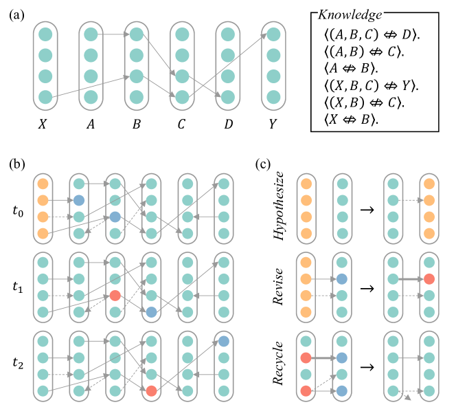
Figure 1: Model diagram. (a) An example of the learned network. There are six concepts, $A$ through $D$, $X$, and $Y$. Each concept is represented as a column that contains multiple nodes. There are links between nodes. Multiple links constitute a chain, representing a group of knowledge. For instance, chain “$(A^{(1)},B^{(1)},C^{(3)},D^{(4)})$” represents three beliefs, “$\langle(A,B,C)\mathrel{\Leftrightarrow\!\!\!\!\!\!/\ }D\rangle.$”, “$\langle(A,B)\mathrel{\Leftrightarrow\!\!\!\!\!\!/\ }C\rangle.$”, and “$\langle A\mathrel{\Leftrightarrow\!\!\!\!\!\!/\ }B\rangle.$”. (b) An example of inference procedure. It shows the internals of the model at three consecutive time-steps. At $t_{0}$, concept $X$ is activated. Since there is no context, all the nodes are activated. It anticipates $A^{(2)}$ and $B^{(3)}$ to occur for the next time-step. Node $A^{(2)}$ is not anticipated even if there is a link from $X^{(3)}$ to $A^{(3)}$, because the truth-value (i.e., the strength of the link) is too low. At $t_{1}$, concept $B$ is activated. Node $B^{(3)}$ is activated due to the anticipation, while the other $nodes$ in $B$ remain silent. In the meantime, $C^{(3)}$ is anticipated. Similarly, at $t_{2}$, $C^{(3)}$ is activated, and $Y^{(1)}$ is anticipated. (c) The learning mechanism. When there is no link between two concepts, some links are built as hypotheses (see Sec. 2.2.1). When one or two nodes at both ends of a link are activated, the truth-value in the link is revised according to distinct situations (see Sec. 2.2.2). When the number of links exceeds a threshold, one or some of them are deleted (see Sec. 2.2.3).

2.1 Representation

It is explained above why to use such a representation, and the formal description is given in this sub-section. Generally speaking, the model can be illustrated by two languages, a neural one and a logical one. A more abstract representation, called Graph representation, is used to describe the model. The correspondence of the terms with respect to the three representations is shown in Tab. 1.

2.1.1 Neural Representation

As we see in Fig. 1, there are some columns containing several nodes. Each node represents an artificial (spiking) neuron, which has three possible states, i.e., resting (or non-active) state, depolarized (or predictive) state, and active state, the meanings of which are similar to those in spiking neurons [16]. A neuron in the predictive or resting state transfers into the active state once it is stimulated to some degree, while one in the resting state turns into predictive state if stimulated. In this paper, the former case is called that a neuron is pre-activated for short, and latter case is that a neuron is activated. Inspired by HTM [7], the model here owns the structure of mini-column and follows the same activation rule as in HTM.

A mini-column is a special structure in neocortex [12], and it looks like a column of neurons. Each neuron in a mini-column is activated in a certain or several contexts, as shown in Fig. 1. An event’s occurring corresponds to the activation of a mini-column. When activating a mini-column, if all the neurons within it are non-active, then all the neurons should be activated, meaning that all possible contexts are concerned. In contrast, if there are any neurons in predictive state, then only these neurons becomes active while remaining other neurons to be non-active, meaning that certain contexts occur.

Formally, suppose the $i$th neuron in mini-column $c$, in which there are $n_{c}$ neurons, is denoted by $N_{c}^{(i)}$. The rule of activating mini-column $c$ is shown in Eq. 1,

$$A_{c}^{(i)}=\left\{\begin{aligned} 1&~{}\text{if}&\forall j\in\{1,...,n_{c}\},\hat{A}_{c}^{(j)}=0\\ 1&~{}\text{if}&\hat{A}_{c}^{(i)}=1\\ 0&~{}\text{if}&\hat{A}_{c}^{(i)}=0,\text{and}~{}\exists j\in\{1,...,n_{c}\},\hat{A}_{c}^{(j)}=1\\ \end{aligned}\right.$$ (1)

where $A_{c}^{(i)}$ indicates the active/resting state of neuron $N_{c}^{(i)}$ ($A_{c}^{(i)}=1$ if in active state, and $A_{c}^{(i)}=0$ if in resting state), while $\hat{A}_{c}^{(i)}$ indicates the depolarized state of neuron $N_{c}^{(i)}$ ($\hat{A}_{c}^{(i)}=1$ if in depolarized state, otherwise, $\hat{A}_{c}^{(i)}=0$).

Neurons are connected by synapses. Each synapse is plastic, meaning that its strength is changeable. Some learning rules regarding synapse were proposed, such as Hebbian learning, STDP, [16]etc. If the strength is greater than a threshold (denoted as $\theta$ here), pre-synaptic neuron’s activation would lead to post-synaptic neuron’s activation, otherwise, the synapse is a potential connection waiting for being strengthened. The depolarization procedure is expressed by Eq. 2,

$$\hat{A}_{c_{1}}^{(i),t}=\left\{\begin{aligned} 1&~{}\text{if}~{}A_{c_{2}}^{(j),t-1}=1~{}\text{and}~{}W_{c_{1}(i)}^{c_{2}(j)}>\theta\\ 0&~{}\text{otherwise}\end{aligned}\right.$$ (2)

where $\hat{A}_{c_{1}}^{(i),t}$ indicates the depolarized state of neuron $N_{c_{1}}^{(i)}$ at time-step $t$, $A_{c_{2}}^{(j),t-1}=1$ denotes the active state of neuron $N_{c_{2}}^{(j)}$ at time-step $t-1$, and $W_{c_{1}(i)}^{c_{2}(j)}$ is the strength of the synapse connecting neuron $N_{c_{1}}^{(i)}$ to neuron $N_{c_{2}}^{(j)}$.

The rule of modifying synaptic strength is not explicitly presented here. Generally speaking, it is similar to Hebbian rule: a synapse is strengthened if its pre-synaptic and post-synaptic neurons are activated simultaneously, and is weakened if only one of the neurons is activated in a short duration. The learning rule in this paper is a variant of Hebbian rule (see Sec. 2.1.2 and Sec. 2.2).

Different from the HTM theory, in which an event is represented by sparse distributed representation [17] , the model in this paper adopts concept-centered representation (see 2.1.2), so that the model can work in a human-understandable way.

2.1.2 Logical Representation

The logical representation in this paper is concept-centered, meaning that an event is represented by a single concept (i.e., a single mini-column instead of a set of mini-columns as in HTM).

In sequence learning, a representation should be highly contextual. However, despite of the biological-plausibility and robustness, there seems to be no strong reason why sparse distributed representation (SDR) is necessary for intelligence. In the meanwhile, how to deal with uncertainty is a challenge in HTM [7]. In principle, a collection of neurons in SDR is equivalent to a concept in Non-Axiomatic Logic (NAL) [8] in some sense. I believe the most critical intuition in HTM is that a mini-column involves a collection of representations under multiple contexts, and each neuron in a mini-column is highly related to a certain context. It is natural to think if we could use a single neuron or mini-column, instead of multiple ones, as a representation, simultaneously preserving the intuition in HTM. From another perspective, each concept in Non-Axiomatic Reasoning System (NARS) [18], an AGI system based on NAL, is weakly contextual, meaning that what concept to be activated is determined by the overall status of the system, while it is not determined directly by what is activated at present. As a result, it is possible that that the current NARS is a good model of consciousness [19], however, it still needs to be improved for sequence learning. By exploiting the logic part of NARS, namely NAL, the model proposed can work with uncertainty, and new representations can be derived via well justified logical rules, promising the interpretability of the model.

The schematic diagram of the representation approach is shown in Fig. 1a. A column is interpreted as a concept. Within each column, there are several nodes. A node is interpreted as a task that is comprised of a statement, a budget, and a truth-value. Statement is the identity of task. A task’s occurring means that the agent is perceiving or feeling something at a certain time. For example, when seeing a red flower, a task which represents the red flower raises up, in other words, it feels the red flower. Truth-value, which represents the extent of the agent’s perceiving or feeling, is composed of two parts, frequency (denoted as $f$) and confidence (denoted as $c$), represented by a two-dimensional tuple $\langle f;c\rangle$. Frequency measures ratio of positive evidence among all observations, and confidence reflects the impact of future evidence. Both $f$ and $c$ indicates the uncertainty of a statement. A node, as a task, is also an event in NAL since its truth-value is time-dependent. Budget represents the extent of computation resources allocated to a task; it is highly related to an agent’s attention. An event, in this sense, is not what occurs outside the mind but the subjective experience of the occurrence. Even though a single concept corresponds to multiple events, under a certain context, usually there should be only one or very few events to be activated, so that only part of meanings of the concept is utilized.

The temporal relations between two concepts $E_{1}$ and $E_{2}$ include predictive implication “$\langle E_{1}\mathrel{\Rightarrow\!\!\!\!\!\!\!/\ }E_{2}\rangle$”, retrospective implication “$\langle E_{2}\mathrel{\Rightarrow\!\!\!\!\!\!\!\backslash\ }E_{1}\rangle$”, and predictive equivalence “$\langle E_{1}\mathrel{\Leftrightarrow\!\!\!\!\!\!/\ }E_{2}\rangle$”. A sequence of events can be represented as “$(E_{1},E_{2},...,E_{n})$”.

As shown in Fig. 1a, a chain of nodes represents multiple beliefs simultaneously. For example , “$\langle A^{(1)}\mathrel{\Leftrightarrow\!\!\!\!\!\!/\ }B^{(1)}\rangle$”, “$\langle(A^{(1)},B^{(1)})\mathrel{\Leftrightarrow\!\!\!\!\!\!/\ }C^{(3)}\rangle$”, and “$\langle(A^{(1)},B^{(1)},C^{(3)})\mathrel{\Leftrightarrow\!\!\!\!\!\!/\ }D^{(4)}\rangle$” shares the same chain.

Given two events $E_{1}.~{}\langle f_{1};c_{1}\rangle$ and $E_{2}.~{}\langle f_{2};c_{2}\rangle$, and their corresponding occurrence time $t_{1}$ and $t_{2}$ such that $t_{2}<t_{1}$, the temporal induction rules in NAL includes

$$\{E_{1}~{}\langle f_{1};c_{1}\rangle,E_{2}.~{}\langle f_{2};c_{2}\rangle\} \vdash E_{2}\mathrel{\Rightarrow\!\!\!\!\!\!\!/\ }E_{1}~{}\langle F_{ind}\rangle$$ (3)

$$\{E_{1}~{}\langle f_{1};c_{1}\rangle,E_{2}.~{}\langle f_{2};c_{2}\rangle\} \vdash E_{1}\mathrel{\Rightarrow\!\!\!\!\!\!\!\backslash\ }E_{2}~{}\langle F_{ind}^{\prime}\rangle$$ (4)

$$\{E_{1}~{}\langle f_{1};c_{1}\rangle,E_{2}.~{}\langle f_{2};c_{2}\rangle\} \vdash E_{2}\mathrel{\Leftrightarrow\!\!\!\!\!\!/\ }E_{1}~{}\langle F_{com}\rangle$$ (5)

where $F_{ind}$ and $F_{com}$ are induction and functions which map the truth-values of premises to that of conclusion.

For each event, the truth-value is constant (e.g., $\langle 1.0;0.9\rangle$) in this paper, though they could be revised dynamically in future work. The truth-value of an anticipation can be derived by temporal deduction rule in NAL, for example,

$$\{E_{1}~{}\langle f_{1};c_{1}\rangle,E_{1}\mathrel{\Leftrightarrow\!\!\!\!\!\!/\ }E_{2}.~{}\langle f_{2};c_{2}\rangle\}\vdash E_{2}~{}\langle F_{ded}\rangle$$ (6)

where $F_{ded}$ is deduction function. When a concept is activated, that is, a corresponding event “$E.\langle f;c\rangle$” occurs, all the contextual-concepts “$E^{(i)}\langle f^{(i)};c^{(i)}\rangle$” ($i\in{1,...,n}$, where $n$ is the number of contextual-concepts of concept $E$) are observed as a fact represented by a truth-value, so that the revision rule is applied to merge the two truth-values of fact and anticipation. The revision rule in NAL is

$$E\langle f_{1};c_{1}\rangle,E\langle f_{2};c_{2}\rangle\vdash E\langle F_{rev}\rangle$$ (7)

where $F_{rev}$ is revision function. It is implied that an anticipated event has higher $confidence$ when it actually occurs.

When a concept is activated, which contextual-concept to be activated depends on the expectations of the truth-values. In NAL, expectation of statement “$S\langle f;c\rangle$” is

$$e(S)=F_{exp}(f,c)=c(f-0.5)+0.5$$ (8)

We can see that there exists such a threshold $\zeta$, such that the expectation of both an occurring but not anticipated event, or an anticipated but not occurring event, is less than $\zeta$, while the expectation of an occurring and anticipated event is greater than $\zeta$. A contextual-concept is activated when its expectation is greater than $\zeta$, or when all the expectations of contextual-concepts in a concept are less than $\zeta$, i.e.,

$$A_{c}^{(i)}=\left\{\begin{aligned} 1&~{}\text{if}&\forall j\in\{1,...,n_{c}\},e(E_{c}^{(j)})<\zeta\\ 1&~{}\text{if}&e(E_{c}^{(j)})>\zeta\\ 0&~{}\text{if}&e(E_{c}^{(i)})<\zeta,\text{and}~{}\exists j\in\{1,...,n_{c}\},e(E_{c}^{(j)})>\zeta\\ \end{aligned}\right.$$ (9)

The procedure of temporal induction for statement “$E_{c_{1}}^{(i)}\mathrel{\Leftrightarrow\!\!\!\!\!\!/\ }E_{c_{1}}^{(j)}$” happens only when $A_{c_{1}}^{(i)}=1$ or $A_{c_{2}}^{(j)}=1$.

Although predictive implication (“$\mathrel{\Rightarrow\!\!\!\!\!\!\!/\ }$”) and retrospective implication (“$\mathrel{\Rightarrow\!\!\!\!\!\!\!\backslash\ }$”) are also important, as a start point, the model in this paper exploits merely predictive equivalence (“$\mathrel{\Leftrightarrow\!\!\!\!\!\!/\ }$”) for learning and inference.

2.1.3 Graph Representation

We have seen in Sec. 2.1.1 and Sec. 2.1.2 that the model can not only be explained as a neuronal network, but also be interpreted by a logic. However, to better illustrate it, I have to use a more abstract representation (which is called Graph Representation) to avoid conceptual ambiguity in the description, mainly by using the formal language of Graph Theory. As shown in Fig. 1, the basic elements are node and link (a.k.a. vertex and directed edge in Graph Theory). A column (as hyper-vertex) is a collection of nodes. Each link’s weight is adjustable. Each node has three states, activation, non-activation, and pre-activation, each of which is represented by a pair of real numbers (i.e., truth-value in Sec. 2.1.2) ranging from 0 to 1. The states of real number can be binarized by a threshold (see Eq. 9).

The correspondence among the terms in the three representations is shown in Tab. 1.

Graph Repr.	Neural Repr.	Logical Repr.
node	neuron	contextual-concept
column	mini-column	concept
link	synapse	temporal statement (e.g., “$\langle A\mathrel{\Leftrightarrow\!\!\!\!\!\!/\ }B\rangle$”)
link-weight	synaptic strength	truth-value (abbr., t.-v.)
weight adjustment	synaptic plasticity	temporal-induction and revision
activation	active state	event with t.-v. “$(1.0;0.9)$”*1
pre-activation	depolarized state	anticipation with t.-v. “$(1.0;0.9)$”*1
non-activation	resting state	event with t.-v. “$(1.0;0.1)$”*2

• Here in the truth-value, frequency and confidence are both very high, though the concrete values does not have to be the same as $(1.0;0.9)$.

• Here in the truth-value, confidence is very high but frequency does not matter, and the concrete values does not have to be the same as $(1.0;0.1)$.

Table 1: The correspondence of terms among the three representations: Neural Representation, Logical Representation, and Graph Representation.

2.2 Sequence Learning

The challenge is how to construct the links given a series of events. First, there is no way to fully-connect among all nodes (meaning that a node has links connected to all other nodes). Facing an endless list of events, the number columns cannot be pre-determined (thus, new columns should be able to be built up dynamically), and the number of links would explode as the number of columns increases with fully-connection. Due to the Assumption of Insufficient Knowledge and Resources (AIKR) [20], the number of links connected to or from a node should not exceed constant (though it could be either large or small), consequently, there has to be a certain mechanism through which new links are created with old links to be recycled. In Sec. 2.1.2, the logic rules of temporal induction has been introduced, however, when to do induction and to revise the link remains to be answered in the following.

2.2.1 Hypothesizing

Initially, there are no nodes and no links in the network. Whenever an event occurs, the corresponding column is constructed if there does not exist one. Each node in a column has no links at the beginning of its creation. When two columns are activated in succession, two sets of nodes are activated correspondingly. Suppose a set of nodes $\mathcal{N}_{1}$ in column ${C}_{1}$ and a set of nodes $\mathcal{N}_{2}$ in column ${C}_{2}$ are activated, then one node $E_{c_{1}}^{(i)}$ is picked out from $\mathcal{N}_{1}$, and another one $E_{c_{2}}^{(j)}$ from $\mathcal{N}_{2}$, a new link is created connecting from $E_{c_{1}}^{(i)}$ to $E_{c_{2}}^{(j)}$ if there does not exist one. Since the initial weight of the link, represented by truth-value, is very weak, i.e., the confidence is low (e.g., $c=0.1$). The link, represented by “$E_{c_{1}}^{(i)}\mathrel{\Leftrightarrow\!\!\!\!\!\!/\ }E_{c_{2}}^{(j)}\langle 1.0;0.1\rangle$”, in this sense is what we usually mean by hypothesis.

When picking out a node for hypothesizing from a set, which one to pick? Let us consider the meaning of a node. A node is activated given a context of events, thus, intuitively, a node means a concept in a certain context. Ideally, there should be at most one pre-link pointing into it and at most one post-link pointing out from it, and there should at least one link possessed by it. In this case, the node would be activated if and only if one certain context of events occur. For example, a node $B^{(1)}$ is activated only when the sequence “$(A,B,C,D)$” occurs, and $B^{(1)}$ exactly identifies the event $B$ in that context, rather than the $B$ in “$(X,B,C,Y)$”. However, due to AIKR, the number of nodes should be a constant, so that a node has to serve for multiple different contexts. We can say the meaning of a node is clear or unambiguous, either if it has a post-link with strength much greater than other post-links, and a pre-link with strength much greater than other pre-links, or if one of its pre-link and post-link is much greater than its other links. To pick out one for hypothesizing, the overall principle is to avoid as far as possible to do harm to the clear meaning of a node. The concrete strategy in this paper is to pick out a node with the lowest utility. Here, the utility of node $E_{c}^{(i)}$ is defined as

$$u(E_{c}^{(i)})=1-(1-u_{1})(1-u_{2})$$ (10)

where

$$u_{1} =\left\{\begin{aligned} &0&,&~{}\text{if}~{}\mathcal{L}_{pre}(E_{c}^{(i)})=\varnothing\\ &\max_{\forall L\in\mathcal{L}_{pre}(E_{c}^{(i)})}e(L)&,&~{}\text{otherwise}\end{aligned}\right.,~{}\text{and}$$ (11)

$$u_{2} =\left\{\begin{aligned} &0&,&~{}\text{if}~{}\mathcal{L}_{post}(E_{c}^{(i)})=\varnothing\\ &\max_{\forall L\in\mathcal{L}_{post}(E_{c}^{(i)})}e(L)&,&~{}\text{otherwise}\end{aligned}\right.$$

where $\mathcal{L}_{pre}(E_{c}^{(i)})$ and $\mathcal{L}_{post}(E_{c}^{(i)})$ are the sets of node $E_{c}^{(i)}$’s pre-links and post-links correspondingly, and $e(L)$ is the expectation of the truth-value of link $L$ (see Eq. 8). Thus, if a node has a much clear meaning, it tends not to be picked out. Though the side effect is that a node, which has ambiguous meaning but has a link with strong strength, is also inclined to be selected, it seems not an issue in practice.

New hypotheses are constantly come up with, though they do not lead to strong conclusion until enough evidences are collected. A too weak hypothesis like “$E_{c_{1}}^{(i)}\mathrel{\Leftrightarrow\!\!\!\!\!\!/\ }E_{c_{2}}^{(j)}\langle 1.0;0.1\rangle$” leads to non-activation of its consequent $E_{c_{2}}^{(j)}$, according to Eq. 9, in this sense, a hypothesis is a potential link between two nodes. This potential link is similar to a synapse with a low strength. Only when the strength is greater than a threshold, the synapse can be viewed as truly connected and can transit signals between two neurons. Nevertheless, a link can be strengthened whether it is strong or weak, so that a hypothesis has chance to become stronger and cause the activation of its consequent given the activation of its antecedent.

2.2.2 Revising

Whenever a column is activated, one link is picked out for revising. The general principle to enhance the link is that is the most probable to become conclusive. Specifically, the selected link $L$ is

$$L=\underset{{\forall L\in\mathcal{L}_{pre}(E_{c}^{(i)}),\forall i\in\{1,...,n_{c}\}}}{\mathrm{argmax}}e(L)$$ (12)

meaning that it picks out a link with the maximal expectation from all the pre-links of all the nodes within a column. As a result, a link represented by statement “$E_{c_{1}}^{(i)}\mathrel{\Leftrightarrow\!\!\!\!\!\!/\ }E_{c_{2}}^{(j)}$” is selected for revising.

Given two nodes $E_{c_{1}}^{(i)}$ and $E_{c_{2}}^{(j)}$ which are concerned on, the temporal induction rule is applied to revise the truth-value of statements including “$E_{c_{1}}^{(i)}\mathrel{\Leftrightarrow\!\!\!\!\!\!/\ }E_{c_{2}}^{(j)}$”, according to Eq. 3 and Eq. 7. The difference in the learning procedure is that some negative evidences are obtained if an anticipated event does not occur. Specifically, node $E_{c_{2}}^{(j)}$ (as consequent) is in the state of pre-activation at time-step $t$ (i.e., $\hat{A}_{c_{2}}^{(i),t}=1$) if node $E_{c_{1}}^{(i)}$ (as antecedent) is in the state of activation at time-step $t-1$ (i.e., $A_{c_{1}}^{(i),t-1}=1$), and the expectation of statement “$E_{c_{1}}^{(i)}\mathrel{\Leftrightarrow\!\!\!\!\!\!/\ }E_{c_{2}}^{(j)}$” is greater than a threshold $\theta$, i.e.,

$$\hat{A}_{c_{2}}^{(i),t}=\left\{\begin{aligned} &1&,&~{}\text{if}~{}A_{c_{1}}^{(i),t-1}=1,~{}\text{and}~{}e(E_{c_{1}}^{(i)}\mathrel{\Leftrightarrow\!\!\!\!\!\!/\ }E_{c_{2}}^{(j)})>\theta&\\ &0&,&~{}\text{otherwise}&\end{aligned}\right.$$ (13)

An event usually may have multiple causes and effects, however, in the sequence learning model, It is possible to build causal chains in which each event has at most only one cause and at most one effect in a certain context. Therefore, in the case of $\exists j\in\{1,...,n_{c}\},e(E_{c}^{(j)})>\zeta$ (i.e., the current event has a certain context, such that one or some of nodes within a column are activated but not all), if node $E_{c_{2}}^{(j)}$ is anticipated ($\hat{A}_{c_{2}}^{(i),t}=1$) but not activated (${A}_{c_{2}}^{(i),t}=0$), then some negative evidences of $E_{c_{2}}^{(j)}$ are collected. Similarly, when node $E_{c_{2}}^{(j)}$ is activated, all of its possible causes are paid attention to. If an antecedent $E_{c_{1}}^{(i)}$ is not activated before $E_{c_{2}}^{(j)}$, given statement “$E_{c_{1}}^{(i)}\mathrel{\Leftrightarrow\!\!\!\!\!\!/\ }E_{c_{2}}^{(j)}$”, then some negative evidences of $E_{c_{2}}^{(j)}$ are also collected. Otherwise, the two nodes are activated in succession, temporal induction can be applied directly.

There is also a punishment in the case $\forall j\in\{1,...,n_{c}\},e(E_{c}^{(j)})<\zeta$ (i.e., all the nodes within a column are activate without being anticipated first). If the whole column is activated, a bunch of anticipations would occur. For those anticipations which are not verified later, a slight amount of evidences are collected by $w^{-}=|\{e(L)>\theta,\forall L\in\mathcal{L}_{post}(E_{c_{1}}^{(i)})\}|+b$, where the first term denotes the number of $E_{c_{1}}^{(i)}$’s post-links each of whose expectation is greater than threshold $\theta$, and the second term $b$ is a constant (e.g., $b=40$); here, threshold $\theta$ and constant $b$ are hyper-parameters of the model. When $b=\infty$, it means no penalty for this case.

2.2.3 Recycling

Again due to AIKR, the number of links regarding a node should not exceed a certain threshold, otherwise, some of the links should be dropped. This is related to the forgetting process of memory.

Pre-links $\mathcal{L}_{pre}(E_{c_{1}}^{(i)})$ and post-links $\mathcal{L}_{post}(E_{c_{1}}^{(i)})$ of node $E_{c_{1}}^{(i)}$ are stored in a priority queue, sorted by utility. In the current design, utility of a link is determined by the expectation of its truth-value. When the number of link $n_{L}$ in the priority queue is greater than a certain threshold $\xi$ (e.g., $\xi=100$), the exceeding part is recycled, i.e., $(n_{L}-\xi)$ links with the lowest priorities are deleted.

Utility probably not only depends on the expectation of a link’s truth-value, but also some other factors. For example, a link may be reserved in a short period after it is newly created, though its expectation is much less than some long-standing links (see Future Work for more discussion in Sec. 4).

3 Results

Since the tasks, sequence prediction and sequence generalization, are equivalent to each other, while the sequence recognition task can be reduced to prediction[2], the test-cases in this paper only involves sequence prediction. In the meanwhile, sequence decision making task [2] can be considered as associated with much more complex procedures of intelligence, thus, decision making is not considered in this paper, though the model proposed in this paper is the foundation of further work.

The model is tested on some synthetic datasets. Different from typical approach for evaluating machine learning methods, there is no explicit division between training set and test set here, since it is considered that the learning process is online and life-long: each sample observed by an agent is not only a training sample but also a test one, and current experience is not necessary to be similar to the past, that is to say, no stable distribution of data is assumed.

The data for tests are manufactured in the following way. Suppose there are $n_{r}$ types of events; each event is labeled by a term, such as characters like “$A$”, “$B$”, “$X$”, and strings like “e0347”, “e1001”, which identifies the type of an event. Whatever a term looks like for human developers, it is just the name of a concept inside the system, a concept whose meaning merely depends on its acquired (rather than predetermined) relations with other concepts, as suggested in Non-Axiomatic Logic (NAL) [8]. A dataset in this paper is a list of events, which contains sequences like “$(...,A,B,C,D,...)$”, “$(...,X,B,C,Y,...)$”, and so on. Some events are determined by their predecessors, for example, in a given situation, event “$B$” is always followed by “$C$” but comes after either “$A$” or “$X$”; event “$D$” follows “$(A,B,C)$”, but given merely “$(B,C)$”, either “$D$” or “$Y$” is expected to occur. Besides, other events are randomly generated, leading to the whole list of events unpredictable to some extent.

With this form of input data, three aspects are considered for evaluating the model, capacity (see Sec. 3.1), catastrophic forgetting (see Sec. 3.2), and capability (see Sec. 3.3), though the capability aspect is analyzed only in theory.

3.1 Capacity Tests

Evaluating the capacity of the model is related to two factors, the number of sequences and the length of a sequence that is expected to be recognized. In a test, datasets are generated, within the prototype of “$(\$,...,\$,E_{1},...,E_{m},\$,...,\$)$”, where $E_{1},...,E_{m}$ are deterministic events which keep the same in every sample of the prototype, while “$\$$” is the unpredictable variable, which varies from sample to sample; The dataset’s parameter $m$ denotes the number of deterministic events for each sequence. There are $p$ pieces of prototypes of sequences to be generated. When an event occurs, the model anticipates some events to occur for the next step. If an event is anticipated and occurs immediately, then we can say the event is correctly anticipated. The proportion of the number of truly anticipated events within a certain past period (e.g., the past 100 time-steps) is the anticipation accuracy of the current time-step.

Firstly, a simple case is tested. Suppose each event is named by a single character (from $A$ to $Z$), so that there are $26$ possible types of events for the model. The dataset contains two prototypes of sequences “$(\$,\$,A,B,C,D,E,\$)$” and “$(\$,\$,X,B,C,D,Y,\$)$”, where “$\$$” denotes a random event. In this case, $m=5$ and $p=2$), and only $50\%$ of the events are deterministic and can be predicted very well. The test results are shown in Fig. 2. Figure 2(a) shows the accuracy of anticipation as time goes by. At each time-step, there could be multiple anticipations, and Fig. 2(b) shows the number of events anticipated by the model – ideally, there should be only one anticipated event if the system is pretty sure what context it observes; multiple anticipated events implies that the system retains the possibility of several contexts. We can see that around 2 events are anticipated on average for each time-step. Figure 2(c) shows the number of activated nodes in the model – generally speaking, a node’s activation means a certain context is recognized by the model. The fewer nodes are active, the clearer the context is. It shows in Fig. 2(c), there are around $2$ nodes activated on average for each time-step.

Secondly, the model is tested with different options of length $m$ and the number of prototypes $p$, and even the different numbers of types of events. The proportions of unpredictable events in the datasets are all $50\%$. As shown in Fig. 3, the model has proper anticipations on future events. With $m=5$ and $p=5$ (see Fig. 3(a)), as well as $m=14$ and $p=20$ (see Fig. 3(d)), the anticipation accuracy in either cases is greater than $50\%$, exceeding the theoretically highest accuracy (the same as that shown in Fig. 2(a)). This is because The model learns some patterns from the random events. The number of anticipated nodes and that of active nodes are both no more than $2$ in each of the two cases.

A probably simpler setting for the model is that the number of types of events is much greater than $26$. The test results are shown in Fig. 3(g)-3(i), where the number of types $n_{r}$ is $1000$. We can see that the the accuracy is closely around $50\%$, and the number of anticipated nodes and that of active nodes are both around $1$. The model performs better in this setting than the previous ones, because in the previous tests, one type of event most probably engages in multiple prototypes of sequences, so that the model may be confused; while in this test, the types of events are much greater, so that one type of event get a higher chance to be involved in a single context, consequently, it is much easier to memorize and distinguish different patterns for the model.

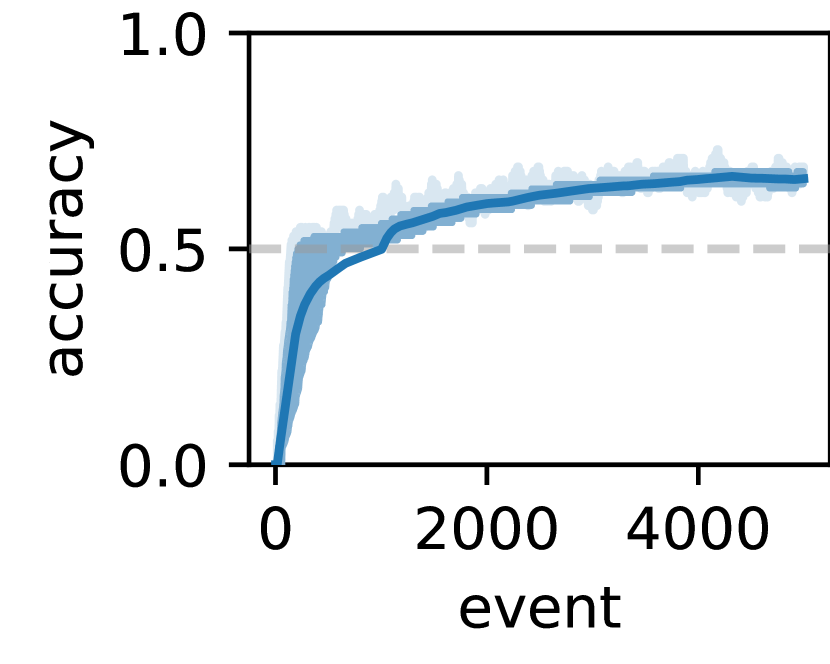
(a)

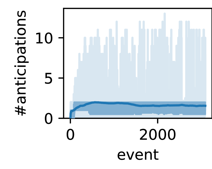
(b)

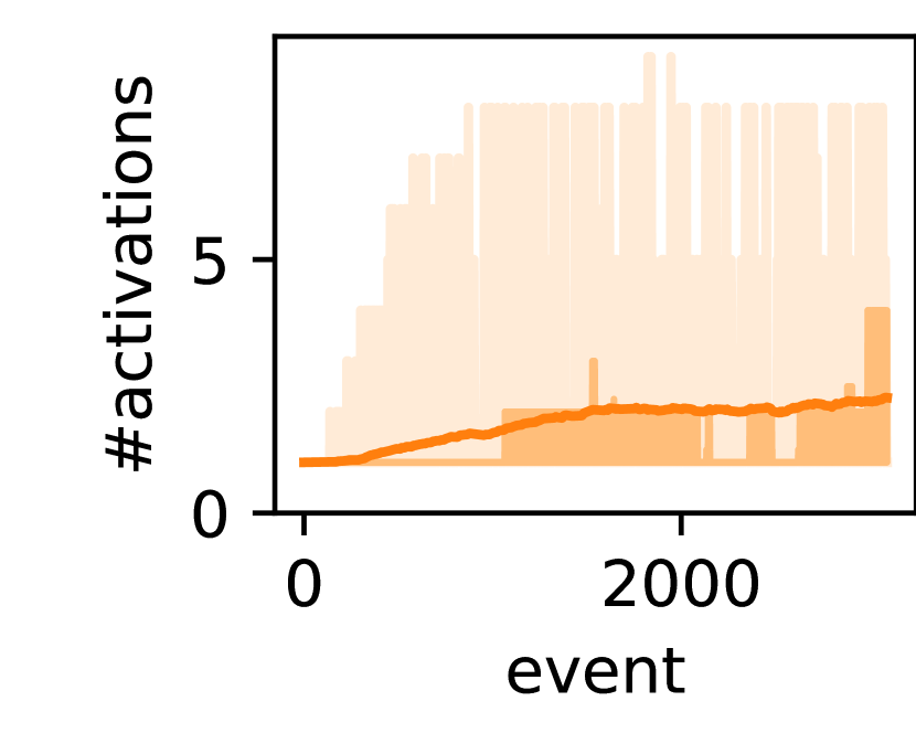
(c)

Figure 2: Capacity-Test results for the simple case, where the prototypes of sequences are “$(\$,\$,A,B,C,D,E,\$)$” and “$(\$,\$,X,B,C,D,Y,\$)$”, where “$\$$” denotes a random event. (a) The accuracy of anticipation. (b) The number of anticipations. (c) The number of active nodes.

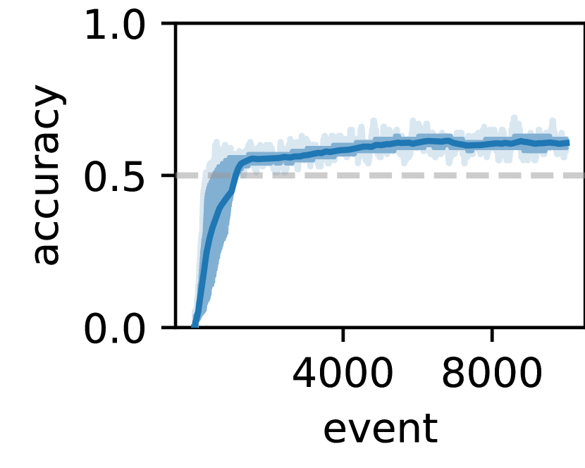
(a)

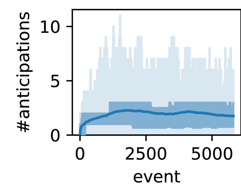
(b)

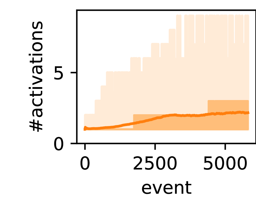
(c)

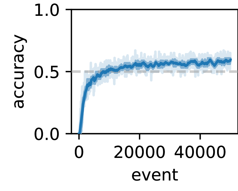
(d)

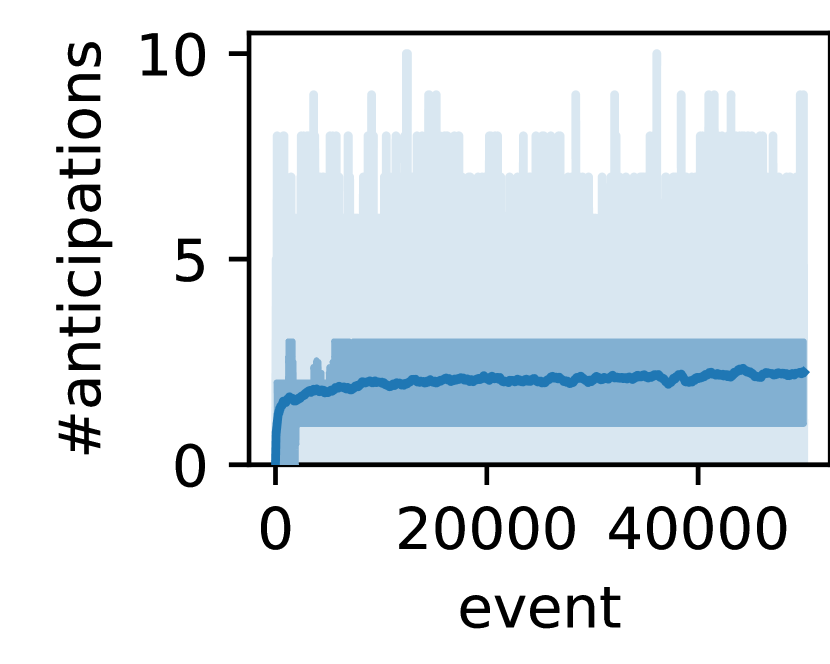
(e)

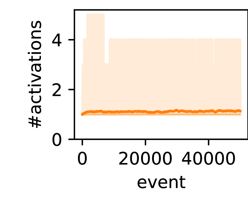
(f)

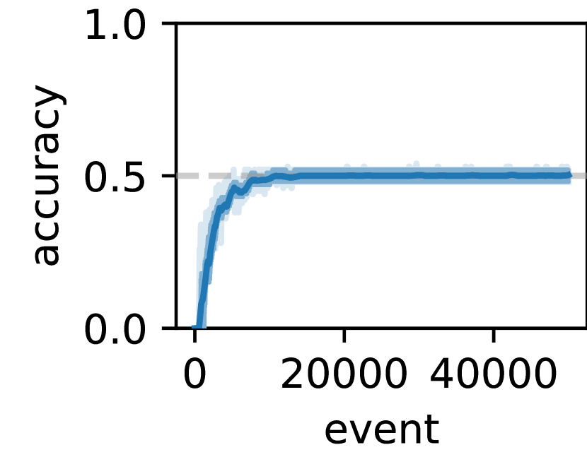
(g)

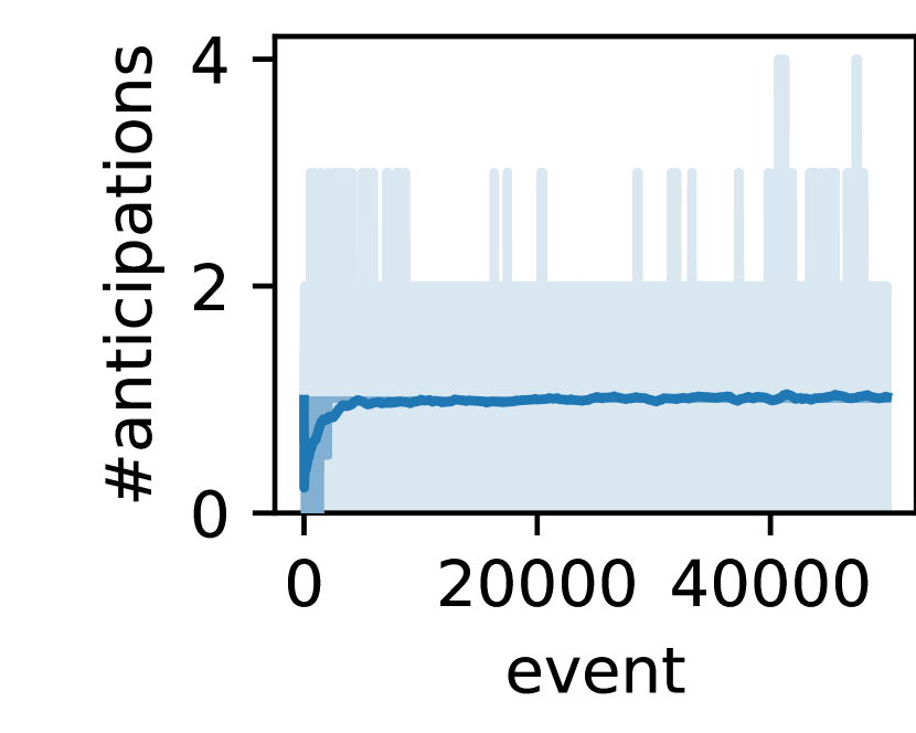
(h)

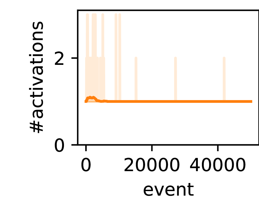
(i)

Figure 3: Capacity-Test results with different options of length $m$ and the number of prototypes $p$, and event the different numbers of types of evens. (a), (b), and (c) are test results with $m=5$, $p=5$, and $26$ types of events. (d), (e), and (f) are test results with $m=14$, $p=20$, and $26$ types of events. (g), (h), and (i) are test results with $m=14$, $p=20$, and $1000$ types of events.

3.2 Catastrophic Forgetting Tests

The issue of catastrophic forgetting (also known as catastrophic interference) was proposed by McCloskey and Cohen in 1989 [15], pointing out that distributed representation of connectionist networks (a.k.a. Deep Neural Networks nowadays) have a non-desirable property that modifications on new data interfere the memory for old data, leading to forgetting large amount of the previous experience. Some modern research (e.g., [21]) over the years still tried to solve this issue.

Since the model in this paper adopts concept-centered representation (see Sec. 2.1.2), this annoying property seems probably not to occur in theory. However, due to relatively insufficient resources of memory and computation [20] assumed in this paper, the model has to remember something new and forget something old, thus, acquiring new knowledge is possible to interfere old one, and the extent of interference should be evaluated (at least qualitatively if not quantitatively), to see whether it is catastrophic.

The test results of catastrophic-forgetting is shown in Fig. 4 and Fig. 5. With $26$ types of events (in Fig. 4) or $1000$ types (in Fig. 5), in an episode, $20$ prototypes of sequences with length $14$ for each are generated. The patterns vary across different episodes. After seeing three episodes one by one, the model encounters the previous episodes repeatedly. If there existed catastrophic forgetting in the model, then we would have seen the anticipation accuracy fell down significantly when seeing an episode with the same patterns once again. However, that does not happen in Fig. 4 and Fig. 5. Therefore, qualitatively speaking, the model does not suffer from catastrophic forgetting.

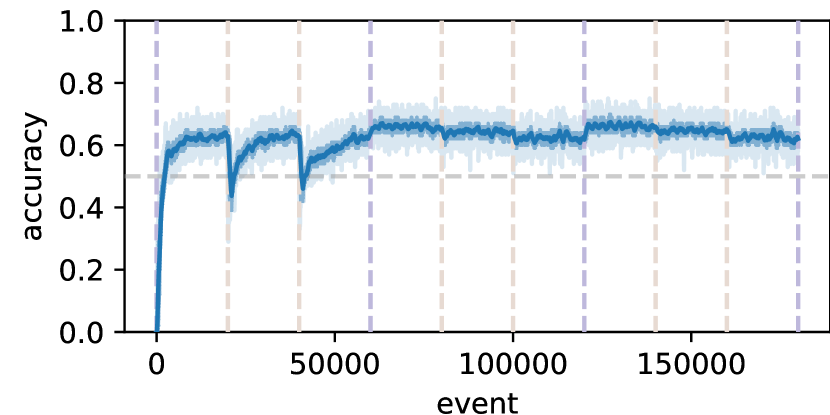
(a)

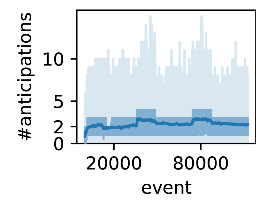
(b)

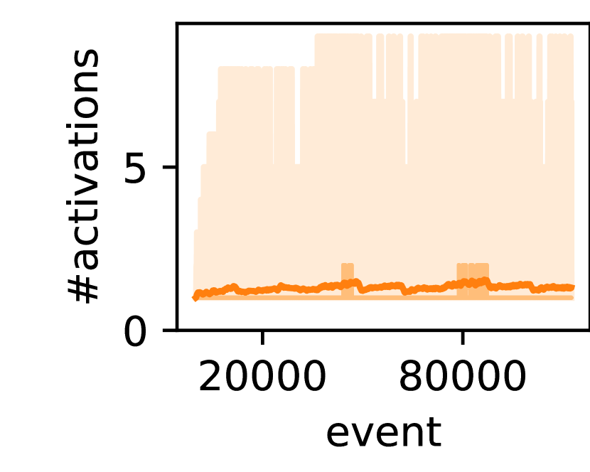
(c)

Figure 4: Results of catastrophic forgetting test when the number of concepts $n_{r}=26$ (see Sec. 3.2 for more details).

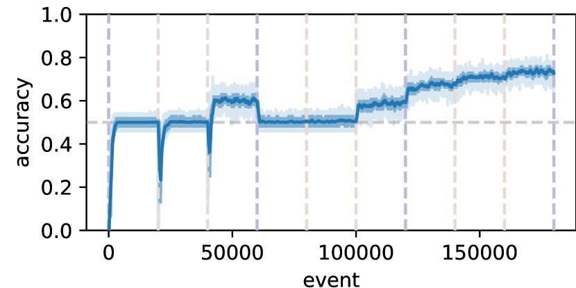
(a)

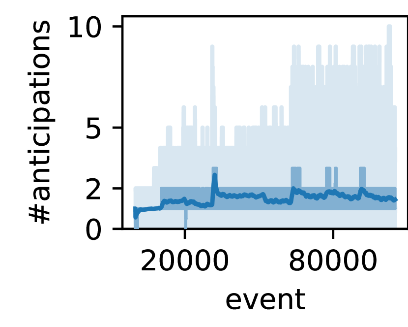
(b)

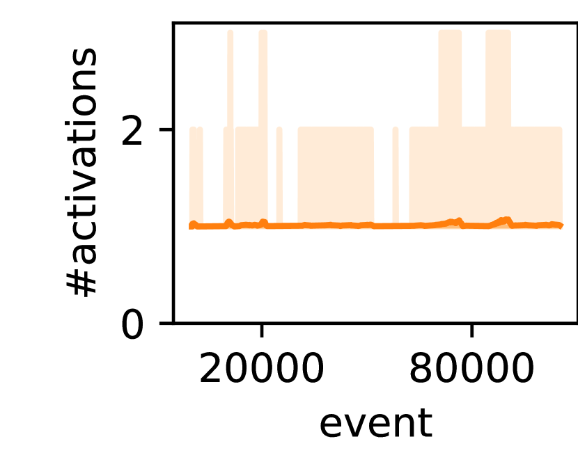
(c)

Figure 5: Results of catastrophic forgetting test when the number of concepts $n_{r}=1000$ (see Sec. 3.2 for more details).

3.3 Capability Analysis

The bound of the model’s capability needs to be clarified. First, the model is not an AGI system, although it can be considered as a first step on modeling the complex unity of intelligence. Second, the model focuses on an aspect of intelligence, i.e., sequence learning. Third, in the current design, the model can only deal with the situation where merely one single event appears at a certain time-step; the case where multiple events appear simultaneously is not the target in this paper. Forth, the time interval of any pair of events is a constant; this assumption on the interval enables the model to deal with some situations where the order of events matters but time interval does not; an example of this kind of situations is natural language processing. Part of future work is to expand the capability of the model (see Future Work in Sec. 4).

Inside the bound, the model is capable of learning patterns in an endless list of events. In the meanwhile, the model is enabled by the power of Non-Axiomatic Logic to handle uncertainty. This property (i.e., being able to handle uncertainty) is directly derived in theory, thus, no test is needed to prove that in practice, and exploiting the property is more related to applications of the model.

4 Discussion

A Principle

From the learning mechanism proposed in this paper, the following principle can be summarized:

Computational resources tend to converge toward knowledge with lower levels of uncertainty.

Specifically, in the model, a link with higher truth-value gets a greater chance to be enhanced. This principle is not a novel idea. It could be a guidance for designing AI systems, and it is also observed in biological systems: In neuroscience and neuronal dynamics, the well-known winner-take-all rule [22, 16, 23] shares the same intuition. In psychology, Piaget’s theory suggests that new information input to a subject is incorporated into already existing knowledge[24]. In other words, the existing knowledge will be allocated computational resources to give a meaning to the content. Earlier, in ancient China, as it is said in Tao Te Ching, “The Way of Nature reduces excess and replenishes deficiency. By contrast, the Way of Humans is to reduce the deficient and supply the excessive.” The learning process of the model proposed exactly follows the Way of Humans.

Brain-inspired Structure

Even if the model is inspired by human brain, in AI systems, it still needs the answer why it should be of the structure like that, rather than a trivial answer as “because brain looks like that”. The reason why the mini-column structure work is that it represents a concept with distinct meanings under different contexts. A neuron in a mini-column is activated because part of the meanings of the corresponding concept is recalled. Neurons are connected as a chain, representing concepts organized as a sequence. Due to the Assumption of Insufficient Knowledge and Resources (AIKR), the total number of links should not exceed a constant, so a balance between memorizing and forgetting does matter. Based on this view, the learning mechanism in Sec. 2.2 is designed.

Hierarchy

We can see that the model is capable of distinguishing the patterns with the same head and tail but different middle parts, e.g., “$(A,B,C,D)$” and “$(X,B,C,Y)$”, however, I do not think it learns a hierarchical structure from a sequence. A pattern is implicitly stored in the memory, in the form of chain, rather than tree in computer science. “Chunk” is the basis of building a hierarchy [1], and a chain could be a hint or heuristic to form a chunk. As suggested in previous work (e.g., [25] and [25]), forming hierarchical representations of sequences benefits for accessing and self-repairing sequences learned. The model proposed suffers from the problem of memorizing a long sequential pattern: a long chain is broken into smaller ones in the learning procedure, as a result, some events in a long sequence cannot be anticipated correctly as expected. This problem, I believe, can be solved by imposing hierarchical structure to the model – Nodes in a chain are combined as a chunk (i.e., a compound in NAL [8]), which simultaneously serves as a column and is processed in the same way as what is done in this paper.

Causal Inference

Due to that temporal implication or equivalence in NAL has the meaning of prediction, a link can be viewed as a basic form of causation [11], and a chain in this paper corresponds to what is called causal chain. The model, with no prior knowledge in the beginning, tries to summarize causal relations among events, and those links with high certainty are reserved; this procedure is also called causal discovery. Although, by backtracking a link or chain, causal explanations can be obtained, there are causal explanations that are much more complex in human’s daily experience. This issue is too big to be discussed detailly in this paper, nevertheless, I believe this is a novel start point to address the issue of causal inference.

Neuronal Basis of Logic

How does logic emerge from human brain? There are two possibilities, one is that neural networks might learn something which is called logic, the other is that neuron’s activity could be interpreted as logic. Evidently, the work in this paper supports the latter one, though it does not negate the previous one. We can see in Sec. 2.1 and Tab. 1 that the model can be illustrated in both two ways, a neural one and a logical one. The correspondence between membrane voltage of a neuron and truth-value of a statement is not discussed deliberately, though I guess there would emerge some valuable work on this issue.

Dropping out the Black-box of Sequence Learning

This paper proves the potential of learning patterns of sequences based on a logic, the problem which was addressed well by purely statistical models (e.g., Hidden Markov Models [4]), neurodynamics models (e.g., HTM [7], spiking neural networks [26]), and neural networks (e.g., RNN [5]). The model is fully interpretable by a logic, Non-Axiomatic Logic [8], as a result, human developers are capable of explaining the system’s behaviors by recording, in a human-understandable way, and checking its internal activities. It provides an alternative besides well-performed but inexplicable models, especially neural networks that are widely criticized as black boxes.

Comparison

The previous pieces of work are valuable, but there are still some differences from this model. The practical performances of various models are not compared in this paper, majorly due to two reasons. First, of course, the model proposed here is a preliminary one and is not powerful enough. As suggested above, at least a hierarchy should have been learned by the model to deal with some complex situations. Thus, it does not make much sense to apply it to some complex tasks, such as natural language processing. Second, there are some different theoretical assumptions in this paper. It assumes that the types of events are unknown to a system before it is initialized, as a result, corresponding representations should be generated in the run-time. In typical Hidden Markov Models [4], the types of events should be pre-specified and cannot be changed when a system starts running. In neural networks, it usually assumes that data are known satisfactorily to a system, so that the system can see the the whole data set repeatedly. In this work, the assumption is that the data set is endless, thus, the model has to do learn in real time. Besides, the interpretability of the model is an attractive property. The performance of the model proposed is similar to HTM [7], though they adopt quite different theoretical foundations. There are some advantages of distributed representations in HTM, for example, robustness to noise and damage. In contrast, by adopting the concept-centered representation, uncertainty can be represented naturally.

Future Work

There is a great deal of work to be done in the future, related to either improving the sequence learning model per se or modeling other intelligence phenomena upon the model proposed.

On one hand, apart from introducing the hierarchical structure mentioned above, the major improvement might involve the competition among links. In the current design, links compete with each other based on its utility, however, utility of a link should have depend on several factors besides its expectation, such as time that a link is established (more specifically, a link built in the recent time tends not to be forgot, even if its expectation is low), the goal of a system (therefore, there should be a top-down interaction with the model), and so on. In addition, predictive implication and retrospective implication have not been considered much in the current design, and the learning mechanism could be modified to improve the efficiency of learning. Certainly, the current design of the model is not perfect enough. For example, in Fig. 3(b), I hope the number of anticipations should be close to $1$, meaning that the system clearly know the context it locates in. The current result shows that there are around $2$ possible contexts, and the system cannot determine which is correct exactly, though it knows to some extent.

On the other hand, sequence learning could be the basis of sensorimotor learning, where the input is high-dimensional data (typically, 2-D image), and an agent perceives its environment by glimpsing different places (a.k.a. eye-movement). How to built a interpretable sensorimotor learning model seems a big challenge. Also, multiple events might occur simultaneously, and how to deal with concurrent events deserves further research.

5 Conclusion

In this paper, a model of sequence learning is proposed. The model exploits Non-Axiomatic Logic (NAL) [8] as the basis of representation, inference, and learning. The model is brain-inspired since the structure is highly inspired by Hierarchical Temporal Memory (HTM) [7], which mimics the mini-columns in neocortex [12], though mini-column is imposed of a special meaning (i.e., concept in NAL) in this paper. A learning algorithm is designed, comprising of three steps: hypothesizing, revising, and recycling – Due to the Assumption of Insufficient Knowledge and Resources (AIKR) [20], there is no way to memorize the whole dataset (to do offline learning [14]) as well as all possibilities of sequences, in the mean while, the time complexity should be a constant when handling each event input to the system. The hypothesizing and recycling procedures are responsible for resources allocation, to guarantee that the model satisfies AIKR. In the revising procedure, candidate links are picked out for temporal induction and revision that are logical rules in NAL. To predict future events, temporal deduction rule is applied to generate anticipations. The model can be converted to Narsese, the formal language of NAL, so that the model is fully interpretable, explainable, and even trust-worthy.

The dataset for test is assumed to be an endless list of events, meaning that theoretically there is no explicit head or tail of the list; thus, the model has to do the so called online learning [14] and work in real-time in a sense. The dataset is generated synthetically, with $50\%$ predictable events and $50\%$ random events. For the predictable part, a certain number (denoted as $p$) of prototypes of sequences are generated; each of the prototype has a certain length (denoted as $m$). To test the capacity of the model, with different $m$s and $p$s, the model is asked to make anticipations on next events. The correctness of anticipations is plotted in Fig. 2 and Fig. 3, showing that the model performs well in several settings with different requirements for capacity. In addition, another task, a.k.a. continual learning [21], is used to test whether the model suffers from catastrophic forgetting [15], which is a long-standing problem in models with distributed representation, such as neural networks. The problem of catastrophic forgetting does not occur in the model proposed, as shown in Fig. 4 and Fig. 5. This is because the model exploits logical representation (or concept-centered representation, see 2.1.2), through which modifying one concept or its relevant connections does not intervene other irrelevant concepts, though forgetting is inevitable due to insufficient resources.

This paper demonstrates the potential of learning sequential patterns in a logical way, though there is some interesting work for further researching.

Declarations

Supplementary information

The source code is available at “https://github.com/bowen-xu/SeL-NAL”.

Acknowledgments

I thank those who reviewed this article for their suggestions; especially, I discussed a lot with my advisor, Dr. Pei Wang, on the idea and the work proposed in this paper, and I appreciate his comments and advice.

References

- \bibcommenthead
- Conway [2012] Conway, C.M.: Sequential learning. In: Seel, N.M. (ed.) Encyclopedia of the Sciences of Learning Sequential Learning, pp. 3047–3050. Springer, LLC, 233 Spring Street, New York, NY 10013, USA (2012)
- Sun and Giles [2001] Sun, R., Giles, C.L.: Sequence learning: From recognition and prediction to sequential decision making. IEEE Intelligent Systems 16(4), 67–70 (2001)
- Clegg et al. [1998] Clegg, B.A., DiGirolamo, G.J., Keele, S.W.: Sequence learning. Trends in Cognitive Sciences 2(8), 275–281 (1998) https://doi.org/10.1016/S1364-6613(98)01202-9
- Rabiner and Juang [1986] Rabiner, L., Juang, B.: An introduction to hidden markov models. IEEE ASSP Magazine 3(1), 4–16 (1986) https://doi.org/10.1109/MASSP.1986.1165342
- Medsker and Jain [2001] Medsker, L.R., Jain, L.: Recurrent neural networks. Design and Applications 5, 64–67 (2001)
- Vaswani et al. [2017] Vaswani, A., Shazeer, N., Parmar, N., Uszkoreit, J., Jones, L., Gomez, A.N., Kaiser, Ł., Polosukhin, I.: Attention is all you need. Advances in neural information processing systems 30 (2017)
- Hawkins and Ahmad [2016] Hawkins, J., Ahmad, S.: Why neurons have thousands of synapses, a theory of sequence memory in neocortex. Frontiers in neural circuits, 23 (2016)
- Wang [2013] Wang, P.: Non-axiomatic Logic: A Model of Intelligent Reasoning. World Scientific, Singapore (2013)
- Harnad [1990] Harnad, S.: The symbol grounding problem. Physica D: Nonlinear Phenomena 42(1-3), 335–346 (1990)
- Wang [2005] Wang, P.: Experience-grounded semantics: a theory for intelligent systems. Cognitive Systems Research 6(4), 282–302 (2005)
- Wang and Hammer [2015] Wang, P., Hammer, P.: Issues in temporal and causal inference. In: Artificial General Intelligence: 8th International Conference, AGI 2015, AGI 2015, Berlin, Germany, July 22-25, 2015, Proceedings 8, pp. 208–217 (2015). Springer
- Buxhoeveden and Casanova [2002] Buxhoeveden, D.P., Casanova, M.F.: The minicolumn hypothesis in neuroscience. Brain 125(5), 935–951 (2002)
- Wang [2001] Wang, P.: Confidence as higher-order uncertainty. In: Proceedings of the Second International Symposium on Imprecise Probabilities and Their Applications, Ithaca, New York, pp. 352–361 (2001)
- Hoi et al. [2021] Hoi, S.C., Sahoo, D., Lu, J., Zhao, P.: Online learning: A comprehensive survey. Neurocomputing 459, 249–289 (2021)
- McCloskey and Cohen [1989] McCloskey, M., Cohen, N.J.: Catastrophic Interference in Connectionist Networks: The Sequential Learning Problem. In: Bower, G.H. (ed.) Psychology of Learning and Motivation vol. 24, pp. 109–165. Academic Press, ??? (1989)
- Gerstner et al. [2014] Gerstner, W., Kistler, W.M., Naud, R., Paninski, L.: Neuronal Dynamics: From Single Neurons to Networks and Models of Cognition. Cambridge University Press, Cambridge (2014)
- Hawkins et al. [2016] Hawkins, J., Ahmad, S., Purdy, S., Lavin, A.: Biological and machine intelligence (bami). Initial online release 0.4 (2016)
- Hammer et al. [2016] Hammer, P., Lofthouse, T., Wang, P.: The opennars implementation of the non-axiomatic reasoning system. In: Artificial General Intelligence: 9th International Conference, AGI 2016, New York, NY, USA, July 16-19, 2016, Proceedings 9, pp. 160–170 (2016). Springer
- Wang [2020] Wang, P.: A constructive explanation of consciousness. Journal of Artificial Intelligence and Consciousness 7(02), 257–275 (2020)
- Wang [2019] Wang, P.: On defining artificial intelligence. Journal of Artificial General Intelligence 10(2), 1–37 (2019)
- Zeng et al. [2019] Zeng, G., Chen, Y., Cui, B., Yu, S.: Continual learning of context-dependent processing in neural networks. Nature Machine Intelligence 1(8), 364–372 (2019)
- Riesenhuber and Poggio [1999] Riesenhuber, M., Poggio, T.: Hierarchical models of object recognition in cortex. Nature Neuroscience 2(11), 1019–1025 (1999)
- Lee et al. [1999] Lee, D.K., Itti, L., Koch, C., Braun, J.: Attention activates winner-take-all competition among visual filters. Nature Neuroscience 2(4), 375–381 (1999)
- Müller et al. [2015] Müller, U., Ten Eycke, K., Baker, L.: Piaget’s Theory of Intelligence. In: Goldstein, S., Princiotta, D., Naglieri, J.A. (eds.) Handbook of Intelligence: Evolutionary Theory, Historical Perspective, and Current Concepts, pp. 137–151. Springer, New York, NY (2015)
- Lashley [1951] Lashley, K.S.: The problem of serial order in behavior. In: Cerebral Mechanisms in Behavior; the Hixon Symposium, pp. 112–146. Wiley, Oxford, England (1951)
- Liang et al. [2020] Liang, Q., Zeng, Y., Xu, B.: Temporal-sequential learning with a brain-inspired spiking neural network and its application to musical memory. Frontiers in Computational Neuroscience 14, 51 (2020)