Optimal Shrinkage Estimation of Fixed Effects in Linear Panel Data Models

Abstract

Shrinkage methods are frequently used to estimate fixed effects to reduce the noisiness of the least squares estimators. However, widely used shrinkage estimators guarantee such noise reduction only under strong distributional assumptions. I develop an estimator for the fixed effects that obtains the best possible mean squared error within a class of shrinkage estimators. This class includes conventional shrinkage estimators and the optimality does not require distributional assumptions. The estimator has an intuitive form and is easy to implement. Moreover, the fixed effects are allowed to vary with time and to be serially correlated, and the shrinkage optimally incorporates the underlying correlation structure in this case. In such a context, I also provide a method to forecast fixed effects one period ahead.

1 Introduction

Linear panel data models commonly include fixed effects to allow for unobserved heterogeneity. The fixed effects capture information about heterogeneity that is often empirically relevant, and thus fixed effects themselves are a parameter of interest in a number of studies. Following the work of Abowd et al. (1999), the literature on the analysis of wage differential factors has focused on employer (and employee) fixed effects in a linear panel specification with wages as the outcome. In the literature on teacher valued-added (Rockoff, 2004; Rothstein, 2010; Chetty et al., 2014a), student test scores are regressed on student characteristics along with a teacher fixed effect, and this fixed effect is interpreted as a measure of teacher quality. Other examples include the effects of neighborhoods on intergenerational mobility (Chetty and Hendren, 2018), judges on sentence length (Kling, 2006), schools on student achievement (Angrist et al., 2017), and hospitals on patient outcomes (Hull, 2020).

Researchers typically estimate a large number of fixed effects, such as one for each firm in a given economy or for each teacher in a school district. However, the effective sample size available for the estimation of each fixed effect is relatively small: a single employer can hire only so many employees, and a single teacher can teach only so many students. Formally, in the asymptotic experiment, the number of fixed effects often grows to infinity, but the sample size corresponding to each fixed effect remains finite. If the researcher uses the least squares estimator—the coefficient on the dummy variables for the fixed effect units under the corresponding OLS specification—one ends up with a large number of noisy estimates.

To resolve this problem, applied researchers have used estimators that shrink the least squares estimator using an Empirical Bayes (EB) method. Such EB estimators are derived under a hierarchical model. The model assumes that the true fixed effect is drawn from a normal distribution with unknown moments. These moments are called hyperparameters. The least squares estimator conditional on the true fixed effect is also assumed to follow a normal distribution, centered at the true fixed effect with known variance. Under this model, the mean of the true fixed effect conditional on the least squares estimator (i.e., the posterior mean) provides a class of shrinkage estimators indexed by the hyperparameters. The hyperparameters determine the degree of shrinkage, where the least squares estimators with lower variances get shrunk by less. In the EB framework, the hyperparameters are tuned by maximizing the marginal likelihood of the least squares estimator implied by the hierarchical model. Since the hyperparameters are tuned using the distributional assumptions made in the hierarchical model, the risk properties of EB estimators are inherently sensitive to these assumptions.

I provide an alternative shrinkage estimator with optimality properties that do not rely on such distributional assumptions. Moreover, I allow the fixed effects to vary with time and to be serially correlated within each unit. While it seems natural for the fixed effects to vary with time, allowing such time drift in the fixed effects makes the least squares estimator even noisier, which is possibly one reason such a specification has not been used often. The proposed shrinkage method takes into account the underlying correlation structure, and pools the information across time in a way that minimizes the risk of the estimator. In particular, the EB estimator used under the assumption of time-invariant fixed effects is a special case of the proposed estimator. With the proposed procedure, the data decides whether or not to use this estimator. In this context of time-varying fixed effects, I also provide an optimal forecast method to predict the fixed effect one period ahead. A special case of this forecast method is the estimator used by Chetty et al. (2014a).

The derivation of the proposed estimator starts from the same hierarchical model that the EB method employs. However, unlike in the EB approach, the model is used only to restrict the class of estimators to those defined by the posterior mean. Once the class of estimators is narrowed down, no further reference is made to any of the distributional assumptions imposed by the hierarchical model. The hyperparameters are chosen so that the corresponding estimator minimizes an estimate of the mean squared error (MSE), which is the risk criteria I use throughout the paper. I refer to this estimate of the risk as the unbiased risk estimate (URE). The URE estimator chooses the hyperparameters to minimize the URE.

I show that the URE converges to the true loss in a suitable sense. This convergence between the risk estimate and the true risk implies the (asymptotic) optimality of the URE estimator within the class of estimators under consideration. This class includes, for example, the conventional EB methods used in the literature. Also, while the least squares estimator does not belong to the class of estimators I consider, a simple approximation argument shows that the URE estimator weakly dominates this estimator as well.

The optimality of the estimator holds under only mild regularity conditions, and thus is robust to the distributional assumptions that EB methods rely on. In particular, the normality assumptions on the true fixed effects and on the least squares estimator are not required. The normality of the true fixed effect is usually difficult to justify. For the least squares estimator, normality could be plausible if the sample size available for a given fixed effect is large enough to make a central limit theorem argument. However, this is not typically the case. For example, in datasets used in the teacher value-added literature, many teachers are linked to fewer than fifteen students.

Another implicit assumption made by EB methods is that the mean (i.e., the true fixed effect) and variance of the least squares estimator are independent. This rules out the existence of factors that affect both the true fixed effect and the variance of the least squares estimator, which can happen, for example, in the presence of conditional heteroskedasticity. Also, in the teacher value-added model, the variance term of the least squares estimator for the fixed effect of a teacher is inversely proportional to the number of the students the teacher has taught. Hence, if there is any relationship between the number of students in a teacher’s class and the teacher’s value-added, the EB assumption is violated. Likewise, this assumption is violated in the employee-employer matched data setting if bigger firms pay higher wages. The URE estimator is robust to such violations.

To show the optimality of the URE estimator, I derive new results in a multivariate normal means setting. This setting has a natural connection with the least squares estimator. The normal means problem is the problem of estimating the mean vectors $\{\theta_{j}\}_{j=1}^{J}$ upon observing $y_{j}\overset{\mathrm{indep}}{\sim}N(\theta_{j},\Sigma_{j})$ with $y_{j}\in\mathbf{R}^{T}$ and $j=1,\dots,J$. Under heteroskedasticity, in the sense that $\Sigma_{j}$ varies with $j$, no estimator has been shown to be risk optimal (in a frequentist sense) unless $T=1$, which has been dealt with by Xie et al. (2012). Allowing for $T>1$ and general forms of $\Sigma_{j}$, I derive an estimator that obtains the best possible MSE within a certain class of estimators in this model. This result can be applied beyond the estimation of fixed effects. In any context with a large number of parameters and an (approximately) unbiased estimator of these parameters, my method can be used to reduce the MSE.

Simulation results demonstrate the effectiveness of the URE estimator. While all theoretical results rely on asymptotic arguments, the URE estimator shows desirable risk properties even for moderate sample sizes. Across all scenarios with sample sizes of at least 600, the MSE of the URE estimator is within 10% of the best possible MSE. Moreover, the results show that the risk reduction relative to the EB methods can be substantial when the distributional assumptions of the EB methods are not met. For some scenarios, this reduction is as large as 80%. This reduction comes at a relatively small price; even when the EB assumptions are met exactly, the risk of the URE estimator is at most 5% greater than that of the EB estimator. Moreoever, the simulation results also demonstrate favorable performance of the proposed method compared to a nonparametric EB methods in scenarios the current paper is concerned about.

I use the proposed method to estimate a teacher value-added model using administrative data on the public schools of New York City. This analysis indicates that the choice of the estimator makes a significant difference in policy-related empirical results, and that it is crucial to allow for the fixed effects to vary with time. I revisit the policy exercise of releasing the bottom 5% of teachers according to the estimated fixed effects. I find that, relative to the conventional methods, the composition of released teachers changes by 25% if the proposed method is used and by 58% if the proposed forecast method is used. Moreover, an out-of-sample exercise shows that the average value-added of the teachers released under the forecast method is about 20% lower compared to the case where the conventional estimator is used.

Related literature. There is an abundant literature on the normal means model starting from the seminal papers by Stein (1956) and James and Stein (1961). However, the (frequentist) risk properties of James–Stein type estimators in the heteroskedastic normal means model have been considered only recently by Xie et al. (2012). Xie et al. (2012) consider the problem of estimating the univariate, heteroskedastic normal means model by minizing a risk estimate. Subsequently, Xie et al. (2016), Kong et al. (2017), Kou and Yang (2017), and Brown et al. (2018) use a similar approach in different settings, providing optimal shrinkage estimation methods. My paper provides an optimal shrinkage procedure for a normal means model that has not been considered in the literature, using similar URE methods introduced in such papers. Unlike the previous papers that require tuning at most two scalar hyperparameters, here the hyperparameter includes a $T\times T$ positive semidefinite matrix and possibly an additional vector of length $T$. When $T=1$, the proposed method reduces to the methods of Xie et al. (2012) and Kou and Yang (2017). More recently, Banerjee et al. (2020) and Chen (2022) develop nonparametric EB methods under heteroskedasticity that is possibly correlated with the mean.

Recently, there has been increased interest in EB and shrinkage methods in econometrics. While the present paper does not use an EB approach in its strict sense, the class of estimators I consider is inspired by an EB setting. Also, the URE estimators fall into the category of shrinkage estimators, though it seems that this specific form has not been considered in the literature. Hansen (2016) provides a method to shrink maximum likelihood estimators to subspaces defined by nonlinear constraints and derives risk properties of the resulting estimator. In a related setting, Fessler and Kasy (2019) take an EB approach to effectively incorporate information implied by economic theory. For regularized estimation problems, Abadie and Kasy (2019) provide a method of choosing the tuning parameter that gives desirable risk properties. Bonhomme and Weidner (2019) use EB methods to estimate population averages conditional on the given sample, and Liu et al. (2020) use nonparametric EB methods to provide forecasts for the outcome variable in a short panel setting. Armstrong et al. (2020) give robust confidence intervals for EB estimators.

The literature on teacher value-added (Rockoff, 2004; Kane et al., 2008; Rothstein, 2010; Chetty et al., 2014a; see Koedel et al., 2015 for a recent review on the topic) has fruitfully employed EB shrinkage methods to estimate teacher fixed effects. My method can effectively estimate teacher value-added without resorting to restrictive distributional assumptions. Moreover, the value-added is allowed to vary with time. Chetty et al. (2014a) were the first to allow the teacher value-added to change with time. The analysis by Bitler et al. (2019) suggests that it is important to allow for such time-drifts, and my empirical analysis adds evidence for this potential importance. Gilraine et al. (2020) proposes a nonparametric EB approach to estimate value-added by using the methods of Koenker and Mizera (2014). By taking this nonparametric EB approach, they relax the normality assumption on the true fixed effect and consider a broader class of estimators. This approach complements, but does not dominate, the URE methods introduced here, as I discuss in more detail in Section 4.3.

Notation. Let $\{W_{ijt}\}$ be a real (either random or nonrandom) sequence, where the indices take values $j=1,\dots J$, $t=1,\dots,T$, and $i=1,\dots,n_{jt}$ for any $(j,t)$-pair. The following vectors are defined by concatenating the sequence at different levels: $W_{jt}=(W_{1jt},\dots,W_{n_{jt}jt})^{\prime}$, $W_{j}=(W_{j1}^{\prime},\dots,W_{jT}^{\prime})^{\prime}$, and $W=(W_{1}^{\prime},\dots,W_{J}^{\prime})^{\prime}$. The $(j,t)$-level average is written $\overline{W}_{jt}={n^{-1}_{jt}}\sum_{i=1}^{n_{jt}}W_{ijt}$ and the demeaned version of the sequence is defined $\widetilde{W}_{ijt}=W_{ijt}-\overline{W}_{jt}$.

Let $\left\lVert\cdot\right\rVert$ denote the Euclidean norm for both vectors and matrices (i.e., the Frobenius norm in the latter case). For any matrix $A$, $(A)_{ij}$ denotes its $(i,j)$ entry and $\sigma_{k}(A)$ its $k$th largest singular value. By definition, $\sigma_{1}(A)$ is the operator norm of the matrix $A$. Likewise, $\lambda_{k}(A)$ denotes the $k$th largest eigenvalue of a square matrix $A$, so that $\sigma_{k}(A)=\lambda_{k}(A)$ for all $k$ when $A$ is positive semidefinite. Let $\kappa(A)=\sigma_{1}(A)/\sigma_{k}(A)$ be the condition number of any $k\times k$ matrix $A$. For two real symmetric matrices $A$ and $B$, I write $A\geq B$ to denote that $A-B$ is positive semidefinite, with strict inequality meaning that $A-B$ is positive definite. For any $d\in\mathbf{R}^{k}$, let $\mathrm{diag}(d)$ denote the $k\times k$ diagonal matrix with diagonal elements $d$. The set of positive semidefinite $k\times k$ matrices is denoted by $\mathcal{S}_{k}^{+}$, and the $k\times k$ identity matrix is denoted by $I_{k}.$

2 Fixed effects and the normal means model

I consider the following linear panel data model,

$$Y_{ijt}=X_{ijt}^{\prime}\beta+\alpha_{jt}+\varepsilon_{ijt},$$ (1)

where $t=1,\dots,T$, $j=1,\dots J$, and for each $(j,t)$ $i=1,\dots,n_{jt}$. Here, $\{(Y_{ijt},X_{ijt}^{\prime})\}$ denotes the observed data, $\varepsilon_{ijt}$ the idiosyncratic shock, and $\alpha_{jt}$ the time-varying fixed effect which is the object of interest. Typically, $i$ is some individual level, $j$ group level, and $t$ a time dimension. The time-varying fixed effect for $j$, $\alpha_{j}:=(\alpha_{j1},\dots\alpha_{jT})^{\prime}$ is assumed to be independent across $j$ but is allowed to be serially correlated. For the idiosyncratic error terms, assume $\overline{\varepsilon}_{j}=(\overline{\varepsilon}_{j1},\dots,\overline{\varepsilon}_{jT})^{\prime}$ is independent across $j$ and with $\alpha_{j}$, and denote its variance matrix by $\Sigma_{j}$. The variance matrix $\Sigma_{j}$ is assumed known, and in practice a consistent estimator is plugged in under suitable conditions, which does not affect the asymptotic properties.

Example 2.1 (Teacher value-added).

In the teacher value-added model, $j$ corresponds to teacher, $t$ to school year, and $i$ to a student assigned to teacher $j$ in school year $t$. The outcome variable $Y_{ijt}$ is a measure of student achievement (e.g., test score) and $X_{ijt}$ is a vector of student characteristics. The fixed effect $\alpha_{jt}$ is the value-added of teacher $j$ in year $t$, and is considered a measure of teacher quality. I use this model as a running example throughout the paper. For this example, I further assume that $\varepsilon_{ijt}$ is i.i.d across all $i$, $j$, and $t$ with variance $\sigma^{2}_{\varepsilon}$ so that $\Sigma_{j}=\sigma^{2}_{\varepsilon}\mathrm{diag}(1/n_{j1},\dots,1/n_{jT})$. See Koedel et al. (2015) for a recent review on the literature, including a discussion on specification issues.

There are numerous other examples that fall into this framework. In the widely used wage determination model first introduced by Abowd et al. (1999), $j$ corresponds to employer, $t$ to year, and $i$ to employee. In this model, an employee fixed effect is typically included as well. The outcome variable is log wages and the employer fixed effect captures the wage differential due to the employer. In a different, but related setting used in the analysis of neighborhood effects on future economic outcomes by Chetty and Hendren (2018), $j$ corresponds to either commuting zone or county. Here, the outcome variable is some measure of future economic outcome, and the fixed effect captures the effect of the neighborhood one resides in during her childhood to future economic outcome.

All asymptotic arguments are as $J\to\infty$ with $T$ and $n_{jt}$ fixed. This captures the common situation where the number of fixed effects to be estimated is large ($J\to\infty$), with observations for each fixed effect unit being relatively small ($n_{jt}$ remains fixed). In the teacher value-added model, this corresponds to the asymptotic experiment where the number of teachers grows to infinity, with the year dimensions and students per teacher for a given year being fixed. I assume that a consistent estimator $\widehat{\beta}$ of $\beta$ is readily available, which is easy to obtain under standard assumptions such as strict exogeneity (see, for example, Wooldridge, 2010 for a textbook level discussion).

Let $\widehat{\alpha}_{jt}$ denote the least squares estimator for the fixed effects:

$$\widehat{\alpha}_{jt}:=\overline{Y}_{jt}-\overline{X}_{jt}^{\prime}\widehat{\beta}=\overline{X}_{jt}^{\prime}(\beta-\widehat{\beta})+\alpha_{jt}+\overline{\varepsilon}_{jt}=\alpha_{jt}+\overline{\varepsilon}_{jt}+O_{p}(J^{-1/2}).$$

To see the connection between this estimator and the normal means model, note that $\widehat{\alpha}_{j}\to_{d}\alpha_{j}+\overline{\varepsilon}_{j}$ for each $j\leq J$. Further assuming that $\overline{\varepsilon}_{j}$ follows a normal distribution (with variance matrix $\Sigma_{j}$), I have $\left(\alpha_{j}+\overline{\varepsilon}_{j}\right)|\alpha_{j}\sim N(\alpha_{j},\Sigma_{j})$ so that

$$\widehat{\alpha}_{j}|\alpha_{j}\sim N(\alpha_{j},\Sigma_{j}),$$ (2)

approximately.

Note that even if $\varepsilon_{ijt}$ is homoskedastic so that $\operatorname{\mathrm{var}}(\varepsilon_{ijt})=\sigma_{\varepsilon}^{2}$, the variance term of the aggregate term is $\operatorname{\mathrm{var}}(\overline{\varepsilon}_{jt})=\sigma_{\varepsilon}^{2}/n_{jt}$ so that heteroskedasticity is present due to the different cell sizes, $n_{jt}$. Under such heteroskedasticity, it has been noted by Xie et al. (2012) that EB methods do not enjoy the many optimality properties that they do under a homoskedastic setting.

Due to this connection, I now consider the problem of estimating the mean vectors under a multivariate normal means model. The problem is to estimate $\theta=(\theta_{1}^{\prime},\dots,\theta_{J}^{\prime})^{\prime}$ after observing the data $\{y_{j}\}_{j=1}^{J}$ where this is generated according to

$$y_{j}|\theta_{j}\overset{\mathrm{indep}}{\sim}N(\theta_{j},\Sigma_{j}),$$ (3)

for $j=1,\dots,J$ with $y_{j},\theta_{j}\in\mathbf{R}^{T}$. The variance matrix $\Sigma_{j}\in\mathcal{S}_{T}^{+}$ is assumed to be known. This has the exact same structure as the asymptotic approximation of the least squares estimator as seen in (2), with the data $y_{j}$ being the least squares estimator and $\theta_{j}$ the true fixed effect.

3 URE estimators

3.1 Class of shrinkage estimators

The URE estimators will be shown to be optimal within a class of shrinkage estimators, that nests commonly used estimators. The class of estimators corresponds to the Bayes estimators under a hierarchical model. The hierarchical model postulates a Gaussian model on the true mean vector (true fixed effect), which I refer to as a second level model, on top of the Gaussian model on the data (least squares estimator). I emphasize that both normality assumptions are used only to derive the class of estimators.

Consider the second level model

$$\theta_{j}\overset{\mathrm{i.i.d.}}{\sim}N(\mu,\Lambda),$$ (4)

where the location vector $\mu\in\mathbf{R}^{T}$ and the variance matrix $\Lambda\in\mathcal{S}_{T}^{+}$ are unknown hyperparameters to be tuned. The restriction one imposes on $\Lambda$ incorporates the prior knowledge on the underlying covariance structure. I denote by $\mathcal{L}\subset\mathcal{S}_{T}^{+}$ the set that reflects this prior knowledge. As a practical matter, this reduces the dimension of the optimization problem that one must solve to obtain the URE estimators. For example, when $\theta_{j}$ is believed to be covariance stationary, one can take $\mathcal{L}$ as the set of positive semidefinite Toeplitz matrices. This reduces the dimension of $\Lambda$ to $T$ from $T(T+1)/2$ when $\Lambda$ is left unrestricted.

The second level model (4), together with the normal means model (3), gives a hierarchical Bayes model. By standard calculations, the Bayes estimator of $\theta_{j}$ under this model is given as

$$\widehat{\theta}_{j}(\mu,\Lambda):=E[\theta_{j}|y]= \mu+\Lambda(\Lambda+\Sigma_{j})^{-1}(y_{j}-\mu)$$

$$= \left(I_{T}-\Lambda(\Lambda+\Sigma_{j})^{-1}\right)\mu+\Lambda(\Lambda+\Sigma_{j})^{-1}y_{j}$$

Analogous to the univariate case, I refer to $\Lambda(\Lambda+\Sigma_{j})^{-1}$ as the shrinkage matrix. It can be shown that the largest singular value of the shrinkage matrix is less than $1$, justifying the term “shrinkage.” As in the univariate case, noisier observations get more severely shrunken in the sense that $\widetilde{\Sigma}_{j}\leq\Sigma_{j}$ implies $\sigma_{t}(\Lambda(\Lambda+\Sigma_{j})^{-1})\leq\sigma_{t}(\Lambda(\Lambda+\widetilde{\Sigma}_{j})^{-1})$ for all $t=1,\dots,T$. The shrinkage occurs towards the mean of the second level model, $\mu$. In the literature, this is frequently set to $0$ after demeaning the least squares estimators.

Example 3.1 (Independent case).

If $\Lambda=\lambda I_{T}$ and $\Sigma_{j}=\mathrm{diag}(\sigma^{2}_{j1},\dots,\sigma^{2}_{jT})$, then the $t$th component of $\widehat{\theta}_{j}(\mu,\Lambda)$ is given as

$$\left(1-\frac{\lambda}{\lambda+\sigma^{2}_{jt}}\right)\mu_{t}+\frac{\lambda}{\lambda+\sigma^{2}_{jt}}y_{jt},$$

which is the form of shrinkage estimators used in the literature (Rockoff, 2004; Chetty and Hendren, 2018; etc.), with a specific choice of $\lambda$ and $\mu$. Moreover, when $\mu=0$ and $\sigma_{jt}^{2}$ does not vary with $j$, an appropriate choice of $\lambda$ in fact gives the James-Stein estimator.

Example 3.2 (Perfect correlation).

Let $\mathbf{1}$ denote the $T$-vector with all elements equal to $1$. Consider the case where $\Lambda=\lambda\mathbf{1}\mathbf{1}^{\prime}$, which is essentially assuming $\theta_{jt}$ is equal across $t$. Let $\Sigma_{j}=\sigma^{2}\mathrm{diag}(1/n_{j1},\dots,1/n_{jT})$, which corresponds to the linear panel data model with idiosyncratic errors that are homoskedastic and uncorrelated across time. Denote the teacher-level sample size by $n_{j}=\sum_{t=1}^{T}n_{jt}$. In this context, the estimator $\widehat{\theta}(0,\Lambda)$ is given as

$$\lambda\mathbf{1}\mathbf{1}^{\prime}(\Sigma_{j}^{-1}-\Sigma_{j}^{-1}\mathbf{1}(1/\lambda+\mathbf{1}^{\prime}\Sigma_{j}^{-1}\mathbf{1})^{-1}\mathbf{1}^{\prime}\Sigma_{j}^{-1})y_{j}$$

$$= \lambda\mathbf{1}\mathbf{1}^{\prime}\left(\Sigma_{j}^{-1}-\frac{\Sigma_{j}^{-1}\mathbf{1}\mathbf{1}^{\prime}\Sigma_{j}^{-1}}{1/\lambda+\sum_{t=1}^{T}n_{jt}/\sigma^{2}}\right)y_{j}$$

$$= \mathbf{1}\frac{\lambda}{\sigma^{2}/n_{j}+\lambda}\left(\frac{1}{n_{j}}\sum_{t=1}^{T}n_{jt}y_{jt}\right),$$

where the first equality follows by the Woodbury matrix identity.

Note that $\frac{1}{n_{j}}\sum_{t=1}^{T}n_{jt}y_{jt}$ is a weighted mean of the least squares estimators of teacher $j$, and thus is essentially the least squares estimator for the teacher level fixed effect without time drift. This is exactly the estimator used in the majority of the teacher value-added literature with an appropriate choice of $\lambda$. In the proposed method, whether to use this estimator or not is determined in a data driven way, depending on whether this choice of $\Lambda$ indeed minimizes the risk.

To better understand the operation the shrinkage matrix performs to the data, let $UDU^{\prime}$ denote the spectral decomposition of $\Sigma_{j}^{-1/2}\Lambda\Sigma_{j}^{-1/2}$, the signal-to-noise ratio matrix, with $D=\mathrm{diag}(d_{1},\dots,d_{T})$. For simplicity, consider the case with $\mu=0$. It can be shown that

$$\widehat{\theta}_{j}(0,\Lambda)=\Lambda(\Lambda+\Sigma_{j})^{-1}y_{j}=\Sigma_{j}^{1/2}UD(I_{T}+D)^{-1}U^{\prime}\Sigma_{j}^{-1/2}y_{j}.$$

Here, the last $\Sigma_{j}^{-1/2}$ term simply standardizes the data, $y_{j}$, and the first $\Sigma_{j}^{1/2}$ term brings it data back to its original scale and direction. The $UD(I_{T}+D)^{-1}U^{\prime}$ term captures the direction and degree of shrinkage. Specifically, $U^{\prime}$ rotates the standardized data $\Sigma_{j}^{-1/2}y_{j}$ in the direction of the eigenvectors of the signal-to-noise ratio matrix, $D(I_{T}+D)^{-1}$ shrinks this rotated data according to the eigenvalues of the eigenvalues of signal-to-noise ratio matrix, and finally $U$ rotates the data back to its original axes. Note that $D(I_{T}+D)^{-1}$ is indeed a shrinkage term because $D(I_{T}+D)^{-1}=\mathrm{diag}(d_{1}/(1+d_{1}),\dots,d_{T}/(1+d_{T}))$ and $d_{t}/(1+d_{t})\in[0,1)$ for all $t\leq T$. Since both $U$ and $D(I_{T}+D)^{-1}$ depend on $\Lambda$, the choice of $\Lambda$ determines the direction and magnitude of shrinkage. This is in contrast with the univariate case, where tuning $\lambda$ just determines the magnititude of shrinkage.

One class of shrinkage estimators I consider is $\widehat{\theta}(\mu,\Lambda):=(\theta_{1}(\mu,\Lambda)^{\prime},\dots,\widehat{\theta}_{J}(\mu,\Lambda))^{\prime}$, indexed by the hyperparameters $(\mu,\Lambda)$. This class of estimators includes the conventional EB methods, where one proceeds by substituting an “estimator” $(\widehat{\mu}^{\mathrm{EB}},\widehat{\Lambda}^{\mathrm{EB}})$ for $(\mu,\Lambda)$. This is done by using the marginal distribution of the data implied by the hierarchical model, $y_{j}\overset{\text{indep}}{\sim}N(\mu,\Lambda+\Sigma_{j})$, either by maximum likelihood or the method of moments. I denote the EB maximum likelihood estimator (EBMLE) by $\widehat{\theta}^{\mathrm{EBMLE}}=\widehat{\theta}(\widehat{\mu}^{\mathrm{EBMLE}},\widehat{\Lambda}^{\mathrm{EBMLE}})$ where $(\widehat{\mu}^{\mathrm{EBMLE}},\widehat{\Lambda}^{\mathrm{EBMLE}})$ is tuned by maximizing this marginal likelihood. I also consider another larger class of estimators where each $y_{j}$ is shrunk toward a different location for each $j$, where this location depends on some auxiliary data. This extension is useful when one has additional covariates that can explain $y_{j}$. In the teacher value-added model, this is the case when teacher level covariates are available.

The risk of an estimator $\widehat{\theta}$ of $\theta$ is measured by the compound MSE,

$$R(\theta,\widehat{\theta})=\textstyle\frac{1}{J}\operatorname{\mathbf{E}}_{\theta}(\widehat{\theta}-\theta)^{\prime}(\widehat{\theta}-\theta),$$

where the term “compound” highlights the fact that risks across the independent experiments are aggregated. While I consider only the unweighted case for expositional reasons, all results go through under the weighted compound MSE as long as the weights satisfy a mild boundedness condition, as shown in Appendix E. The expectation $\operatorname{\mathbf{E}}_{\theta}$ is evaluated at $\theta$, and the subscript $\theta$ is omitted unless ambiguous otherwise.

3.2 Risk estimate and URE estimators

Ideally, one would tune the hyperparameters by minimizing the true risk. However, this is infeasible because the risk function depends on the unobserved true mean vectors. Instead, I estimate the risk using Stein’s unbiased risk estimate (SURE) and choose the hyperparameters by minimizing this risk estimate.

To obtain a risk estimate, consider the following unbiased risk estimate which is the SURE formula applied to the estimator $\widehat{\theta}(\mu,\Lambda)$,

$$\mathrm{URE}(\mu,\Lambda)$$

$$:= \frac{1}{J}\sum_{j=1}^{J}\left(\operatorname{\mathrm{tr}}(\Sigma_{j})-2\operatorname{\mathrm{tr}}((\Lambda+\Sigma_{j})^{-1}\Sigma_{j}^{2})+(y_{j}-\mu)^{\prime}[(\Lambda+\Sigma_{j})^{-1}\Sigma_{j}^{2}(\Lambda+\Sigma_{j})^{-1}](y_{j}-\mu)\right),$$

where I define the summand as $\mathrm{URE}_{j}(\mu,\Lambda)$. It is easy to show that $\mathrm{URE}(\mu,\Lambda)$ is indeed an unbiased estimator of the true risk. While SURE applies to any estimator that takes the form $y_{j}+g(y_{j})$ with $g$ being weakly differentiable, normality of $y_{j}$ is crucial for the unbiasedness to hold for all such estimators. However, the function $g$ corresponding to $\widehat{\theta}(\mu,\Lambda)$ is in fact a simple affine function, so that the unbiasedness can be established by a simple bias-variance expansion. Accordingly, the unbiasedness of $\mathrm{URE}(\mu,\Lambda)$ holds without any distributional assumptions on $y_{j}$, apart from the existence of second moments.

Clearly, unbiasedness itself will not guarantee that the estimator obtained by minimizing the risk estimate has good risk properties. In the next section, I show that $\mathrm{URE}(\mu,\Lambda)$ is in fact uniformly close to the true risk, in the sense that minimizing this risk estimate is as good as minimizing the true loss, asymptotically.

I propose three shrinkage estimators that are closely related but differ in the location to which they shrink the data. The estimators are introduced in increasing degrees of freedom. All three estimators are obtained by minimizing a corresponding URE, and thus I refer to such estimators as URE estimators.

Grand mean. The first estimator, which is the simplest, takes $\mu=\overline{y}_{J}:=\frac{1}{J}\sum_{j=1}^{J}y_{j}$ and thus shrinks the data toward the grand mean. The grand mean is an intuitive location to shrink to, and by fixing a value for $\mu$ this method effectively decreases the dimension of the hyperparameters. In the context of fixed effects, if the least squares estimators are demeaned for each time period, it follows that $\overline{y}_{J}=0$. Hence, the estimator shrinks the data toward the origin. Most shrinkage estimators used in the teacher value-added literature shrink the least squares estimator toward the origin. Formally, this estimator is defined as $\widehat{\theta}^{\mathrm{URE},\mathrm{m}}:=\widehat{\theta}(\overline{y}_{J},\widehat{\Lambda}^{\mathrm{URE},\mathrm{m}})$, where

$$\widehat{\Lambda}^{\mathrm{URE},\mathrm{m}}:=\underset{\Lambda\in\mathcal{L}}{\operatorname*{arg\,min}}\,\,\mathrm{URE}(\overline{y}_{J},\Lambda).$$

General location. The second estimator leaves $\mu$ (almost) unrestricted and chooses the location by minimizing the URE. For theoretical reasons, it is not possible to allow for any $\mu\in\mathbf{R}^{T}$ as the centering location. The hyperparameter space for $\mu$ must be restricted so that a certain boundedness property holds. Following a similar idea used by Brown et al. (2018), I restrict $\mu$ to lie in $\mathcal{M}_{J}$, whose definition is given in Appendix A. This URE estimator that shrinks towards a general location, $\widehat{\theta}^{\mathrm{URE},g}$, is defined as $\widehat{\theta}^{\mathrm{URE},g}=\widehat{\theta}(\widehat{\mu}^{\mathrm{URE}},\widehat{\Lambda}^{\mathrm{URE},g})$, where

$$(\widehat{\mu}^{\mathrm{URE}},\widehat{\Lambda}^{\mathrm{URE},g}):=\underset{\mu\in\mathcal{M}_{J},\Lambda\in\mathcal{L}}{\operatorname*{arg\,min}}\mathrm{URE}(\mu,\Lambda).$$

Linear combination of covariates. In the presence of additional data, $Z_{jt}\in\mathbf{R}^{k}$, one can shrink to a linear function of such covariates. In the linear panel data model, these are exactly the covariates that could not be included as explanatory variables because of the $(j,t)$-level fixed effects. Write $Z_{j}=(Z_{j1},\dots,Z_{jT})^{\prime}$. I consider the estimator that shrinks the data toward $Z_{j}\gamma$,

$$\widehat{\theta}^{\mathrm{cov}}_{j}(\gamma,\Lambda):=\left(I_{T}-\Lambda(\Lambda+\Sigma_{j})^{-1}\right)Z_{j}\gamma+\Lambda(\Lambda+\Sigma_{j})^{-1}y_{j},$$

where now $\gamma$ and $\Lambda$ are hyperparameters to be tuned. I denote by $\widehat{\theta}^{\mathrm{cov}}(\gamma,\Lambda)$ the $JT$ vector obtained by concatenating $\widehat{\theta}^{\mathrm{cov}}_{j}(\gamma,\Lambda)$ for $j\leq J$. Define the risk estimate for a given unit $j$ as $\mathrm{URE}^{\mathrm{cov}}_{j}(\gamma,\Lambda)=\mathrm{URE}_{j}(Z_{j}\gamma,\Lambda)$ and the compound risk estimate $\mathrm{URE}^{\mathrm{cov}}(\gamma,\Lambda)=\frac{1}{J}\sum_{j=1}^{J}\mathrm{URE}^{\mathrm{cov}}_{j}(\gamma,\Lambda)$. Then, the estimator is defined as $\widehat{\theta}^{\mathrm{URE},\mathrm{cov}}=\widehat{\theta}^{\mathrm{cov}}(\widehat{\gamma}^{\mathrm{URE}},\widehat{\Lambda}^{\mathrm{URE},\mathrm{cov}})$, where

$$(\widehat{\gamma}^{\mathrm{URE}},\widehat{\Lambda}^{\mathrm{URE},\mathrm{cov}}):=\underset{\gamma\in\Gamma_{J},\Lambda\in\mathcal{L}}{\operatorname*{arg\,min}}\mathrm{URE}^{\mathrm{cov}}(\gamma,\Lambda).$$

Again, $\Gamma_{J}$ is a hyperparemeter space that incorporates restrictions to ensure that URE approximates the true loss well. The precise definition is given in Appendix A.

Example 3.3 (Teacher value-added).

In teacher value-added, teacher (or teacher-year) level covariates are frequently available. Such covariates cannot be used in the initial regression due to the inclusion of the teacher fixed effects. However, one can use such covariates to improve the precision of the teacher fixed-effect estimates. Frequently available teacher level covariates include, for example, gender, tenure, and union status of a teacher. Class size, which is almost always available, is also an example of such covariate. Asymptotically, the inclusion of such covariates are guaranteed to improve the MSE.

While I only consider the simple case of shrinking toward a linear combination of the covariates where the linear combination is defined by the same coefficient $\gamma$ for all time periods, the estimator can be extended in a straightforward manner to allow different coefficients $\gamma_{t}\in\mathbf{R}^{k}$ for each time period $t$. In this case, $y_{j}$ is shrunk toward $(Z_{j1}^{\prime}\gamma_{1},\dots,Z_{jT}^{\prime}\gamma_{T})^{\prime}$. The optimality property to be shown in Section 4 can also be extended to this case with only minor modifications.

Another interesting extension of this estimator is to shrink toward a more general function of the covariates. That is, for a function $m:\mathbf{R}^{k}\to\mathbf{R}$, one can consider shrinking to $(m(Z_{j1}),\dots,m(Z_{jT}))^{\prime}$. The linear case corresponds to the choice $m(z)=z^{\prime}\gamma$. As long as the hyperparameter space for $m$ is totally bounded and satisfies certain regularity conditions, the resulting URE estimator can be shown to optimal in this more flexible class of estimators as well. In practice, one chooses the hyperparameter by minimizing the URE over a sieve space that converges to the hyperparameter space as $J\to\infty$.

Remark 3.1 (Choice of the estimator).

Under some conditions, the three classes corresponding to $\widehat{\theta}^{\mathrm{URE},\mathrm{m}}$, $\widehat{\theta}^{\mathrm{URE},\mathrm{g}}$, and $\widehat{\theta}^{\mathrm{URE},\mathrm{cov}}$ are nested. While $\overline{y}_{J}$ does not necessarily lie in $\mathcal{M}_{J}$, mild regularity conditions on the data ensure that this happens with probability approaching $1$. Also, for an appropriate choice of the constant that defines $\Gamma_{J}$ and including time dummies as covariates, the class of estimators that shrink toward a general location is nested by those that shrink toward $Z_{j}\gamma$. Hence, as $J\to\infty$, $\widehat{\theta}^{\mathrm{URE},\mathrm{cov}}$ is guaranteed to have the smallest risk among the three, according to the optimality result given in the following section. However, this does not guarantee that this is the case in finite samples, and this estimator requires additional data. As a rule of thumb, I recommend using $\widehat{\theta}^{\mathrm{URE},\mathrm{cov}}$ if covariates are available, $\widehat{\theta}^{\mathrm{URE},\mathrm{g}}$ if covariates are unavailable and one has at least a moderate sample size (simulation results imply $J>200$ is enough for $T=4$), and $\widehat{\theta}^{\mathrm{URE},\mathrm{m}}$ otherwise.

4 Optimality of the URE estimators

I show that the URE estimators defined in Section 3.2 asymptotically achieve the smallest possible asymptotic MSE among all estimators in the corresponding class. In particular, this shows that the URE estimators dominate the EB methods, which has been widely used in applied work. The main step in establishing such optimality is to show that the corresponding UREs are uniformly close to the true risk. Since I use an unbiased estimate of risk, this more or less boils down to a uniform law of large numbers (ULLN) argument. I first establish a simple high-level result for a generic URE estimator, and verify that the conditions for this high-level result holds for each of the estimators, under appropriate lower level conditions.

4.1 A generic result

Let $\psi\in\Psi$ denote a generic hyperparameter to be tuned, which can be $\Lambda$, $(\mu,\Lambda)$, or $(\gamma,\Lambda)$ depending on the choice of the estimator, and let $\widehat{\theta}(\psi)$, indexed by $\psi$, denote the shrinkage estimators in consideration. The hyperparameter space $\Psi$ is allowed to depend on the observations and to vary with $J$, as is the case for $\widehat{\theta}^{\mathrm{URE},\mathrm{g}}$ and $\widehat{\theta}^{\mathrm{URE},\mathrm{cov}}$. A generic URE estimator is defined as $\widehat{\theta}^{\mathrm{URE}}=\widehat{\theta}(\widehat{\psi}^{\mathrm{URE}})$, where $\widehat{\psi}^{\mathrm{URE}}$ minimizes $\mathrm{URE}(\psi).$ As a performance benchmark, consider the oracle loss “estimator,” $\widetilde{\theta}^{\mathrm{OL}}=\widehat{\theta}(\widetilde{\psi}^{\mathrm{OL}})$, where

$$\widetilde{\psi}^{\mathrm{OL}}=\underset{\psi\in\Psi}{\operatorname*{arg\,min}}\,\,\ell(\theta,\widehat{\theta}(\psi)).$$

Note that $\widetilde{\theta}^{\mathrm{OL}}$ is not a feasible estimator because it depends on the true $\theta$. However, it serves as a useful benchmark because it minimizes true loss, for any realized $\theta$, and thus no estimator can have strictly smaller loss, and risk, than $\widetilde{\theta}^{\mathrm{OL}}.$ Hence, I refer to $R(\theta,\widehat{\theta}(\widetilde{\psi}^{\mathrm{OL}}))$ as the oracle risk.

The following simple lemma shows that if $\mathrm{URE}(\psi)$ is uniformly close to the true loss in $L^{1}$, then the URE estimator has asymptotic risk as good as the oracle.

Lemma 4.1.

Suppose $\sup_{\psi\in\Psi}\,\,\lvert\mathrm{URE}(\psi)-\ell(\theta,\widehat{\theta}(\psi))\rvert\overset{L^{1}}{\to}0.$ Then,

$$\underset{J\to\infty}{\limsup}\left(R(\theta,\widehat{\theta}^{\mathrm{URE}})-R(\theta,\widetilde{\theta}^{\mathrm{OL}})\right)\leq 0.$$ (5)

Proof.

By definition of $\widehat{\psi}^{\mathrm{URE}}$, I have $\mathrm{URE}(\widehat{\psi}^{\mathrm{URE}})\leq\mathrm{URE}(\widetilde{\psi}^{\mathrm{OL}})$. This gives

$$\ell(\theta,\widehat{\theta}^{\mathrm{URE}})-\ell(\theta,\widetilde{\theta}^{\mathrm{OL}})$$

$$\leq \left(\ell(\theta,\widehat{\theta}^{\mathrm{URE}})-\mathrm{URE}(\widehat{\psi}^{\mathrm{URE}})\right)+\left(\mathrm{URE}(\widetilde{\psi}^{\mathrm{OL}})-\ell(\theta,\widetilde{\theta}^{\mathrm{OL}})\right)$$

$$\leq \,2\sup_{\psi\in\Psi}\lvert\ell(\theta,{\theta}(\psi))-\mathrm{URE}(\psi)\rvert.$$

Taking expectations and then taking $\limsup_{J\to\infty}$ on both sides, the result follows from the $L^{1}$ convergence condition. ∎

Because the left-hand side of (5) cannot be strictly negative due to the definition of the oracle, this in fact shows that the asymptotic risk of the URE estimator is the same as the oracle under the given convergence assumption. Note that the optimality result is conditional on a true mean vector sequence $\{\theta_{j}\}_{j=1}^{\infty}$ such that the uniform $L^{1}$ convergence holds. When establishing the $L^{1}$ convergence for the specific estimators, I impose conditions on the data $\{y_{j}\}_{j=1}^{\infty}$ that ensure such convergence indeed holds.

4.2 Establishing optimality

All three estimators, $\widehat{\theta}^{\mathrm{URE},\mathrm{m}}$, $\widehat{\theta}^{\mathrm{URE},\mathrm{g}}$ and $\widehat{\theta}^{\mathrm{URE},\mathrm{cov}}$, take the form of

$$\widehat{\theta}_{j}(\mu_{j},\Lambda)=\left(I_{T}-\Lambda(\Lambda+\Sigma_{j})^{-1}\right)\mu_{j}+\Lambda(\Lambda+\Sigma_{j})^{-1}y_{j},$$

with different restrictions imposed on $\mu_{j}$. Hence, the difference between the URE and the true loss in all three cases can be written as (see (LABEL:eq:URE_minus_loss_expansion) in Appendix B.1 for the derivation)

$$\begin{aligned} &\frac{1}{J}\sum_{j=1}^{J}\left(\mathrm{URE}_{j}(\mu_{j},\Lambda)-(\widehat{\theta}_{j}(\mu_{j},\Lambda)-\theta_{j})^{\prime}(\widehat{\theta}_{j}(\mu_{j},\Lambda)-\theta_{j})\right)\\ =&\left(\mathrm{URE}(0,\Lambda)-\ell(\theta,\widehat{\theta}(0,L))\right)-\frac{2}{J}\sum_{j=1}^{J}\left(\mu_{j}^{\prime}(\Lambda+\Sigma_{j})^{-1}\Sigma_{j}(y_{j}-\theta_{j})\right).\end{aligned}$$ (6)

An application of the triangle inequality implies that it suffices to show the absolute values of the first and second terms of the right-hand side converge to zero. Then, it follows from Lemma 4.1 that the URE estimators obtain the oracle risk for each class. The first term, which is the difference between the URE and the loss for the estimator that shrinks toward zero, does not depend on $\mu_{j}$ and thus is common for all three estimators. I first show the convergence of this term, and then establish the convergence of the second term for each estimator.

The following assumption states that $y_{j}$’s are independent, the fourth moment of $y_{j}$ is bounded (uniformly over $j$), and that the smallest eigenvalue of the variance of $y_{j}$ is bounded away from zero. I write $y_{j}\sim(\theta_{j},\Sigma_{j})$ to mean that $y_{j}$ follows a distribution such that $\operatorname{\mathbf{E}}y_{j}=\theta_{j}$ and $\operatorname{\mathrm{var}}(y_{j})=\Sigma_{j}$. The supremum $\sup_{j}$ is taken over all $j\geq 1$, and likewise for $\inf_{j}$. Hence, the assumption imposes conditions on the sequences $\left\{\operatorname{\mathbf{E}}\lVert y_{j}\rVert\right\}_{j=1}^{\infty}$ and $\left\{\sigma_{T}(\Sigma_{j})\right\}_{j=1}^{\infty}$.

Assumption 4.1 (Independent sampling and boundedness).

$\mathrm{(i)}\,y_{j}\overset{\mathrm{indep}}{\sim}(\theta_{j},\Sigma_{j})$,
$\mathrm{(ii)}\,\sup_{j}\operatorname{\mathbf{E}}\lVert y_{j}\rVert^{4}<\infty$ and $\mathrm{(iii)}\,0<\textstyle\inf_{j}\sigma_{T}(\Sigma_{j}).$

This assumption is maintained throughout the paper. Note that normality is not required. Accordingly, in the linear panel data model, the idiosyncratic terms are not required to follow a normal distribution. The independence assumption can be relaxed further provided a law of large number goes through for $y_{j}^{\prime}y_{j}$. In the case where $\Sigma_{j}$ is diagonal for all $j$, Assumption 4.1 (iii) boils down to assuming that $\operatorname{\mathrm{var}}(y_{jt})$ is bounded away from zero over $j$ and $t$. Also, in the case where $\Sigma_{j}=\Sigma$ for all $j$, the assumption trivially holds as long as $\Sigma$ is invertible. I note that (ii) implies $\sup_{j}\left\lVert\theta_{j}\right\rVert<\infty$ and $\sup_{j}\operatorname{\mathrm{tr}}(\Sigma_{j})<\infty$ and that (ii) and (iii) together imply $\sup_{j}\kappa(\Sigma_{j})<\infty$, which are implications repeatedly used in the proof.

Example 4.1 (Teacher value-added).

In the teacher value-added model, Assumption 4.1 holds if, for example, (a) $\underline{n}\leq n_{jt}\leq\overline{n}$ for all $j,t$, (b) the true fixed effects are uniformly bounded in magnitude, and (c) the idiosyncratic error term has bounded fourth moment. Since the class size of any teacher is clearly bounded, (a) is easily justified. Typically, the unit of teacher value-added is in standard deviation of the test score, and the test scores are bounded. Hence, as long as the standard deviation of the test scores for each year is strictly positive, which is always the case, (b) is satisfied. The existence of the fourth moment of the idiosyncratic error term, (c), is a mild regularity condition.

The following theorem shows that Assumption 4.1 is enough to ensure uniform convergence of the first term of (LABEL:eq:URE_minus_loss_genmu).

Theorem 4.1 (Uniform convergence of $\mathrm{URE}(0,\Lambda)$).

Suppose Assumption 4.1 holds. Then,

$$\sup_{\Lambda\in\mathcal{S}_{T}^{+}}\left\lvert\mathrm{URE}(0,\Lambda)-\ell(\theta,\widehat{\theta}(0,\Lambda))\right\rvert\overset{L^{1}}{\to}0.$$ (7)

This theorem establishes uniform convergence over the largest possible hyperparameter space for $\Lambda$, $\mathcal{S}_{T}^{+}$, and thus the convergence over any $\mathcal{L}\subset\mathcal{S}_{T}^{+}$ follows. Also, as is clear from the proof, Assumption 4.1 is stronger than necessary. However, I find this stronger set of assumptions not very restrictive with the advantage of being easy to interpret. The proof essentially boils down to establishing a ULLN argument, and then verifying uniform integrability to strengthen the convergence mode from convergence in probability to convergence in $L^{1}$. In fact, Theorem 4.1 implies the asymptotic optimality of the URE method when the centering parameter $\mu$ is taken to equal zero. With this result in hand, I now establish the optimality of each of the three URE estimators by showing that the second term of (LABEL:eq:URE_minus_loss_genmu) converges to zero uniformly in $L^{1}$.

Define the oracle estimators of each class as $\widetilde{\theta}^{\mathrm{OL},\mathrm{m}}$, $\widetilde{\theta}^{\mathrm{OL},\mathrm{g}}$ and $\widetilde{\theta}^{\mathrm{OL},\mathrm{cov}}$, which are the estimators obtained by plugging in the oracle hyperparameters. Specifically, define the optimal hyperparameters as

$$\widetilde{\Lambda}^{\mathrm{OL},\mathrm{m}}:= \operatorname*{arg\,min}_{\Lambda\in\mathcal{S}_{T}^{+}}\ell(\theta,\widehat{\theta}(\overline{y}_{J},\Lambda)),$$

$$(\widetilde{\mu}^{\mathrm{OL}},\widetilde{\Lambda}^{\mathrm{OL},\mathrm{g}}):= \operatorname*{arg\,min}_{(\mu,\Lambda)\in\mathcal{M}_{J}\times\mathcal{S}_{T}^{+}}\ell(\theta,\widehat{\theta}(\mu,\Lambda)),\text{ and}$$

$$(\widetilde{\gamma}^{\mathrm{OL}},\widetilde{\Lambda}^{\mathrm{OL},\mathrm{cov}}):= \operatorname*{arg\,min}_{(\gamma,\Lambda)\in\Gamma_{J}\times\mathcal{S}_{T}^{+}}\ell(\theta,\widehat{\theta}^{\mathrm{cov}}(\gamma,\Lambda)).$$

The, the corresponding estimators are defined as

$$\widetilde{\theta}^{\mathrm{OL},\mathrm{m}}:=\widehat{\theta}(\overline{y}_{J},\widetilde{\Lambda}^{\mathrm{OL},\mathrm{m}}),\,\,\widetilde{\theta}^{\mathrm{OL},\mathrm{g}}:=\widehat{\theta}(\widetilde{\mu}^{\mathrm{OL}},\widetilde{\Lambda}^{\mathrm{OL},\mathrm{g}}),\text{ and }\widetilde{\theta}^{\mathrm{URE},\mathrm{cov}}:=\widehat{\theta}^{\mathrm{cov}}(\widetilde{\gamma}^{\mathrm{OL}},\widetilde{\Lambda}^{\mathrm{OL},\mathrm{cov}}).$$

Grand mean. This estimator shrinks the data toward $\overline{y}_{J}$, which corresponds to taking $\mu_{j}=\overline{y}_{J}$ in the last term of (LABEL:eq:URE_minus_loss_genmu). Hence, the convergence result to be established is

$$\sup_{\Lambda\in\mathcal{S}_{T}^{+}}\left\lvert\frac{1}{J}\sum\nolimits_{j=1}^{J}\overline{y}_{J}^{\prime}(\Lambda+\Sigma_{j})^{-1}\Sigma_{j}(y_{j}-\theta_{j})\right\rvert\overset{L^{1}}{\to}0.$$

Two applications of the Cauchy-Schwarz inequality show that the expectation of the left-hand side is bounded by

$$\left(\operatorname{\mathbf{E}}\lVert\overline{y}_{J}\rVert^{2}\right)^{1/2}\Big{(}\operatorname{\mathbf{E}}\textstyle\sup_{\Lambda}\left\lVert\frac{1}{J}\sum_{j=1}^{J}(\Lambda+\Sigma_{j})^{-1}\Sigma_{j}(y_{j}-\theta_{j})\right\rVert^{2}\Big{)}^{1/2}.$$

The limit supremum, as $J\to\infty$, of the first term is bounded by Assumption 4.1 (ii). For the second term, again a ULLN argument can be used to show that this converges to zero under Assumption 4.1.

Therefore, under Assumption 4.1, it follows that

$$\underset{J\to\infty}{\limsup}\left(R(\theta,\widehat{\theta}^{\mathrm{URE},\mathrm{m}})-R(\theta,\widetilde{\theta}^{\mathrm{OL},\mathrm{m}})\right)=0,$$

and thus the URE estimator obtains the best possible risk within the class. In particular, this class includes the EB methods that shrink to zero after demeaning the fixed effects, and thus establishes that this URE estimator dominates widely used estimators.

Furthermore, the URE estimator also can be shown to dominate the unbiased estimator, $y$, which corresponds to using the least squares estimators without any shrinkage in the context of fixed effects. This is the maximum likelihood estimator (MLE) when the distribution of $y$ is assumed normal. With some abuse of terminology, I refer to this as the MLE even though I am not assuming normality. Because there is no $\Lambda\in\mathcal{S}_{T}^{+}$ such that $\widehat{\theta}(\overline{y}_{J},\Lambda)=y$, the MLE $y$ is not included in the class of estimators I consider. However, a simple approximation argument can be used to establish the dominance.

Suppose there is some sequence $\widetilde{\Lambda}^{\mathrm{MLE}}_{J}$ such that $\widetilde{\theta}^{\mathrm{MLE}}=\widehat{\theta}(\overline{y}_{J},\widetilde{\Lambda}^{\mathrm{MLE}}_{J})$ satisfies

$$\lim_{J\to\infty}\left\lvert R(\theta,\widetilde{\theta}^{\mathrm{MLE}})-R(\theta,y)\right\rvert=0.$$ (8)

Then, it follows that

$$\limsup_{J\to\infty}\left(R(\theta,\widehat{\theta}^{\mathrm{URE}})-R(\theta,y)\right)$$

$$\leq \limsup_{J\to\infty}\left(R(\theta,\widehat{\theta}^{\mathrm{URE}})-R(\theta,\widetilde{\theta}^{\mathrm{MLE}})\right)+\limsup_{J\to\infty}\left(R(\theta,\widetilde{\theta}^{\mathrm{MLE}})-R(\theta,y)\right)\leq 0,$$

where the last inequality follows due to the optimality of $\widehat{\theta}^{\mathrm{URE}}$ and the assumption on $\widetilde{\theta}^{\mathrm{MLE}}$. Hence, finding $\widetilde{\Lambda}^{\mathrm{MLE}}_{J}$ that satisfies (8) is key to establishing that $\widehat{\theta}^{\mathrm{URE},\mathrm{m}}$ weakly dominates $y$. Define $D(\lambda):=\mathrm{diag}(\lambda,\dots,\lambda)$, and note that for any fixed $J$,

$$\lim_{\lambda\to\infty}R(\theta,\widehat{\theta}(\overline{y}_{J},D(\lambda)))=R(\theta,y).$$

Hence, there exists $\lambda_{J}$ such that $\left\lvert R(\theta,\widehat{\theta}(\overline{y}_{J},D(\lambda_{J})))-R(\theta,y)\right\rvert\leq\frac{1}{J},$ and thus taking $\widetilde{\theta}^{\mathrm{MLE}}=\widehat{\theta}(\overline{y}_{J},D(\lambda_{J}))$ satisfies (8). This shows that shrinking the least squares estimator using the URE method cannot do worse than using the least squares estimator, which is a property that EB methods do not have.

General location. This estimator shrinks the data toward a general data-driven location $\mu$, with the restriction that $\mu\in\mathcal{M}_{J}$. The convergence result to be established is

$$\sup_{(\mu,\Lambda)\in\mathcal{M}_{J}\times\mathcal{S}_{T}^{+}}\left\lvert\frac{1}{J}\sum\nolimits_{j=1}^{J}\mu^{\prime}(\Lambda+\Sigma_{j})^{-1}\Sigma_{j}(y_{j}-\theta_{j})\right\rvert\overset{L^{1}}{\to}0.$$

As in the shrinkage to the grand mean case, it follows from Cauchy-Schwarz inequality that the expectation of the left-hand side is bounded by

$$\left(\operatorname{\mathbf{E}}\textstyle\sup_{\mu\in\mathcal{M}_{J}}\lVert\mu\rVert^{2}\right)^{1/2}\Big{(}\operatorname{\mathbf{E}}\textstyle\sup_{\Lambda\in\mathcal{S}_{T}^{+}}\left\lVert\frac{1}{J}\sum_{j=1}^{J}(\Lambda+\Sigma_{j})^{-1}\Sigma_{j}(y_{j}-\theta_{j})\right\rVert^{2}\Big{)}^{1/2}.$$

As mentioned earlier, it can be shown that the second term converges to zero by a ULLN argument under Assumption 4.1, which I show in the proof of Theorem 4.2.

To show that the term $\operatorname{\mathbf{E}}\textstyle\sup_{\mu\in\mathcal{M}_{j}}\lVert\mu\rVert^{2}$ is bounded, note that

$$\operatorname{\mathbf{E}}\textstyle\sup_{\mu\in\mathcal{M}_{j}}\lVert\mu\rVert^{2}=\sum_{t=1}^{T}\operatorname{\mathbf{E}}q_{1-\tau}(\{y_{jt}^{2}\}_{j=1}^{J})$$

by the definition of $\mathcal{M}_{J}$. Hence, it suffices to show $\operatorname{\mathbf{E}}q_{1-\tau}(\{y_{jt}^{2}\}_{j=1}^{J})=O(1)$ for each $t\leq T$. To control the sample quantile behavior of $\{y_{jt}^{2}\}_{j=1}^{J}$, I impose an additional condition. Write $\varepsilon_{jt}:=y_{jt}-\theta_{jt}$ so that $\operatorname{\mathbf{E}}\varepsilon_{jt}=0$ and $\operatorname{\mathbf{E}}\varepsilon_{jt}^{2}=\sigma^{2}_{jt}$, where $\sigma^{2}_{jt}$ denotes the $t$th diagonal entry of $\Sigma_{j}$. Note that $\overline{\sigma}^{2}_{t}:=\sup_{j}\sigma^{2}_{jt}<\infty$ by Assumption 4.1. I assume that the distribution of $\varepsilon_{jt}$ belongs to a scale family with finite fourth moments.

Assumption 4.2 (Scale family).

For each $t$, $\varepsilon_{jt}/\sigma_{jt}\overset{i.i.d.}{\sim}F_{t}$ for $j=1,\dots,J$, where $F_{t}$ is a distribution function with finite fourth moments.

Note that the assumption is notably weaker than requiring that the noise vectors $\varepsilon_{j}$ for $j=1,\dots,J$ belong to a multivariate scale family, which restricts the joint distribution across $t$ in a much more stringent way. Here, I instead require that the error terms belong to a scale family only for each period. It can be shown that, by Assumption 4.1, the problem of bounding $\operatorname{\mathbf{E}}q_{1-\tau}(\{y_{jt}^{2}\}_{j=1}^{J})$ boils down to the problem of bounding $\operatorname{\mathbf{E}}q_{1-\tau}(\{(\varepsilon_{jt}/\sigma_{jt})^{2}\}_{j=1}^{J})$. Then, by Assumption 4.2, this simplifies to bounding the mean of the sample quantile of an i.i.d. sample. I use a result given by Okolewski and Rychlik (2001) to derive a bound on this quantity without having to further impose conditions on the distribution $F_{t}$.

Example 4.2 (Teacher value-added).

In the teacher value-added example, Assumption 4.2 is satisfied as long as the idiosyncratic error terms are i.i.d across $j$ and have finite fourth moment. Hence, this assumption is almost always satisfied in teacher value-added models, or in linear panel data models in general.

The following theorem shows that $\mathrm{URE}(\mu,\Lambda)$ is close to the true loss uniformly over $(\mu,\Lambda)\in\mathcal{M}_{J}\times\mathcal{S}_{T}^{+}$ under this additional assumption.

Theorem 4.2 (Uniform convergence of $\mathrm{URE}(\mu,\Lambda)$).

Suppose Assumptions 4.1 and 4.2 hold. Then,

$$\sup_{\mu\in\mathcal{M}_{J},\Lambda\in\mathcal{S}_{T}^{+}}\left\lvert\mathrm{URE}(\mu,\Lambda)-\ell(\theta,\widehat{\theta}(\mu,\Lambda))\right\rvert\overset{L^{1}}{\to}0.$$

Under homoskedasticity (i.e., $\Sigma_{j}=\Sigma$ for all $j\leq J$), the optimal location parameter for both the URE estimator and the EBMLE estimator is the grand mean, so that $\widehat{\mu}^{\mathrm{URE}}=\widehat{\mu}^{\mathrm{EBMLE}}=\overline{y}_{J}$. This is possibly one reason why the grand mean has been frequently used as the centering location in applied work despite the heteroskedasticity. However, under heteroskedasticity, which is frequently the case in the context of fixed effects, weighing the different observations according to the different variance matrices $\Sigma_{j}$ (and the hyperparameter $\Lambda$) gives better risk properties. Hence, it is recommended that one uses $\widehat{\theta}^{\mathrm{URE},\mathrm{g}}$ rather than $\widehat{\theta}^{\mathrm{URE},\mathrm{m}}$ unless the sample size is relatively small, in which case the additional hyperparameters can result in overfitting.

Linear combination of covariates. This estimator shrinks each observation to a different location, $Z_{j}\gamma$, which depends on the covariate. By a similar calculation given in the case of shrinkage toward a general location, the key step in establishing optimality is to show

$$\left(\operatorname{\mathbf{E}}\textstyle\sup_{\gamma\in\Gamma_{J}}\lVert\gamma\rVert^{2}\right)^{1/2}\Big{(}\operatorname{\mathbf{E}}\textstyle\sup_{\Lambda\in\mathcal{S}_{T}^{+}}\left\lVert\frac{1}{J}\sum_{j=1}^{J}Z_{j}^{\prime}(\Lambda+\Sigma_{j})^{-1}\Sigma_{j}(y_{j}-\theta_{j})\right\rVert^{2}\Big{)}^{1/2}\to 0.$$

Again, the strategy is to show that the first term is bounded and the second term converges to zero. Due to the presence of covariates, the second term is different from that of the previous estimators. Define $\varepsilon_{j}=y_{j}-\theta_{j}$. I make the following assumptions on the covariates.

Assumption 4.3 (Covariates).

$$\mathrm{(i)}\,\, \,\,\textstyle\{(y_{j},Z_{j})\}_{j=1}^{J}\text{ is an independent sample with }Z_{j}\overset{\mathrm{i.i.d,}}{\sim}P_{Z},\hskip 354.12256pt$$

$$\mathrm{(ii)}\, \,\,\textstyle\sup_{j}\sigma_{1}(Z_{j}^{\prime}Z_{j})<\infty\text{ a.s.},\hskip 354.12256pt$$

$$\mathrm{(iii)} \,\,\operatorname{\mathbf{E}}[\varepsilon_{j}|Z_{j}]=0\text{ and }\operatorname{\mathrm{var}}(\varepsilon_{j}|Z_{j})=\Sigma_{j},$$

$$\mathrm{(iv)} \,\,\mu_{Z,2}:=\operatorname{\mathbf{E}}Z_{j}^{\prime}Z_{j}\text{ is nonsingular, and}$$

$$\mathrm{(v)}\, \,\,\textstyle\sup_{j}\operatorname{\mathbf{E}}\,[\lVert y_{j}\rVert^{4}|Z_{j}]<\infty\text{ a.s. }$$

Again, the supremums are taken over all $j\geq 1.$ The independent sampling assumption of (i) is standard. A sufficient condition for (ii) is that there exists some constant $\overline{C}_{Z}\in\mathbf{R}$ such that $\sup_{j,t}\lVert Z_{jt}\rVert<\overline{C}_{Z}<\infty$ almost surely, which amounts to assuming that the covariates are uniformly bounded. The first and second part of (iii) are exogeneity conditions for the first and second moments of the noise term, with respect to the covariates. The full rank condition given in (iv) is standard. The boundedness condition for the conditional expectation given in (v) is a conditional version of Assumption 4.1 (ii). Again, the boundedness conditions in (ii) and (v) can be relaxed to a boundedness condition on the averages of the given quantities.

Note that there is no assumption that states any linear relationship between the covariate matrix $Z_{j}$ and the true mean $\theta_{j}$ and/or $y_{j}$. Hence, there is no such thing as “misspecification” as long as the exogeneity condition (ii) is met. Some specifications yield better risk properties than others, but as long as time dummies are included in the covariates with $B$ being sufficiently large, any specification (choice of covariates) is guaranteed to improve upon $\widehat{\theta}^{\mathrm{URE},\mathrm{g}}$ asymptotically.

Example 4.3 (Teacher value-added).

In the teacher value-added model, $Z_{jt}$ corresponds to teacher-year level covariates. The results here show that, while such covariates could not have been included in the regression formula, such covariates can be used to obtain more accurate estimators of the fixed effects. The exogeneity condition, Assumption 4.3 (ii), is satisfied as long as the covariates are strictly exogenous with respect to the idiosyncratic error terms. This was in some sense already assumed because independence between the fixed effects and the idiosyncratic error terms was assumed. Moreover, note that $n_{jt}$ (or $\Sigma_{jt}$ in general) can be included in $Z_{jt}$, which allows an explicit dependence structure between $\theta_{j}$ and $\Sigma_{j}$.

Now, with some abuse of notation, I condition on a realization $\{Z_{j}\}_{j=1}^{\infty}$ and treat the covariates as fixed. I assume that this fixed sequence satisfies $\sup_{j}\sigma_{1}(Z_{j}^{\prime}Z_{j})<\infty$, $\frac{1}{J}\sum_{j=1}^{J}Z_{j}^{\prime}Z_{j}\to\mu_{Z,2}$, and $\sup_{j}\operatorname{\mathbf{E}}\,[\lVert y_{j}\rVert^{4}|Z_{j}]<\infty$ which holds for almost all realizations due to Assumption 4.3(ii), (iv), and (v), and the strong law of large numbers. I directly impose these conditions on the fixed covariates in the following theorem, with the understanding that such conditions follow from Assumption 4.3. The following theorem shows that the URE is uniformly close to the true loss function over $(\gamma,\Lambda)\in\Gamma_{J}\times\mathcal{S}_{T}^{+}$ under this implied assumption on the covariates, along with the maintained Assumption 4.1.

Theorem 4.3 (Uniform convergence of $\mathrm{URE}^{\mathrm{cov}}(\gamma,\Lambda)$).

Suppose that $\sup_{j}\sigma_{1}(Z_{j}^{\prime}Z_{j})<\infty$, $\lim_{J\to\infty}\frac{1}{J}\sum_{j=1}^{J}Z_{j}^{\prime}Z_{j}=\mu_{Z,2}$, and Assumption 4.1 holds. Then,

$$\sup_{\gamma\in\Gamma_{J},\Lambda\in\mathcal{S}_{T}^{+}}\left\lvert\mathrm{URE}^{\mathrm{cov}}(\gamma,\Lambda)-\ell(\theta,\widehat{\theta}^{\mathrm{cov}}(\gamma,\Lambda))\right\rvert\overset{L^{1}}{\to}0.$$

4.3 Discussion on the optimality results

The optimality of the URE estimators requires only mild conditions on the moments of the data, which is in contrast with the EB estimators that require stringent distributional assumptions to obtain optimality properties. Recall that $y_{j}$ and $\theta_{j}$ correspond to the least squares estimator and the true fixed effect, respectively, in the context of fixed effects. The EB estimators are optimal in the sense of Robbins (1964) when 1) the normality assumptions for both the least squares estimator and the true fixed effect hold and 2) the true fixed effect and variance of the least squares estimator are independent.

The normality assumption on the true fixed effect is typically difficult to justify. Some evidence on the violation of such assumption in the context of teacher value-added is provided in Gilraine et al. (2020). The optimality results here are conditional on a sequence of true mean vectors that is only required to satisfy a mild boundedness condition, and does not rely on such specific distributional assumptions on the true mean vector. The normality assumption on the least squares estimator can be less concerning because one can resort to a central limit theorem argument if the class size $n_{jt}$ is somewhat large. However, this is not necessarily the case in many empirical contexts. For example, there are numerous classes with less than ten students in the data used in Section 7. The optimality result for the URE estimators imposes conditions on the moments of the least squares estimator, leaving the distribution unrestricted.

The independence assumption between the true fixed effect and the variance of the least squares estimator can be easily violated in empirical settings as well. Since the variance of the least squares estimator is inversely proportional to the cell size $n_{jt}$, the assumption is violated if the fixed effect is related with the cell size in some manner. For example, if teachers with higher value-added teach more students, or if the size of the class is related to teaching effectiveness, then such independence is unlikely to hold. Also, if the idiosyncratic error terms are conditionally heteroskedastic with respect to some observed covariates that are correlated with the fixed effects, such independence assumption is again violated. No assumption on the relationship between the mean $\theta_{j}$ and variance $\Sigma_{j}$ is imposed in establishing the optimality of the URE estimators, and thus optimality is guaranteed whether or not the true fixed effect and the variance of the least squares estimators are independent.

It is worth mentioning that the nonparametric EB literature (Jiang and Zhang, 2009; Brown and Greenshtein, 2009; Koenker and Mizera, 2014) provides an alternative method to relax the normality assumption of the true mean, which has been adopted by Gilraine et al. (2020) to the teacher value-added setting. In the nonparametric EB setting, the distribution of the true fixed effect is remained unspecified except for certain regularity conditions. This allows for a significantly wider class of estimators than the class I consider. This approach is complementary to, but does not dominate, the URE approach for two main reasons.

First, the risk properties of the currently available nonparametric EB methods still rely on an independence assumption between the true fixed effect and the variance of the least square estimator (or at least a certain dependence structure between the two) and a normality assumption on the least squares estimators, and therefore there is no guarantee that the nonparametric estimators dominate even asymptotically.

Moreoever, with time-varying fixed effects the nonparametric EB approach involves solving an optimization problem where the argument is a function of $T$ variables, which makes computation very difficult for even moderate values of $T$, and current algorithms are introduced under a univariate (i.e., $T=1$) setting. In Section D, I show that the nonparametric EB gives 30%-170% higher MSE than the proposed estimator under the data generating processes I consider in Section 6.

Remark 4.1 (Unbalanced panel).

While it has been assumed that the given panel data is balanced at the $(j,t)$-level, this is rarely the case in empirical applications. For example, in teacher value-added, only some of the teachers are observed for the entire time span of the data and others appear only in some of the school years. The URE estimators and their optimality can be naturally extended to incorporate this unbalanced case. See Appendix C for details.

5 Summarizing the time trajectory

While the time-varying fixed effects gives more flexibility and contains more information, in some empirical contexts it is still desirable to have a scalar quantity for each $j$ that summarizes the fixed effect for unit $j$. For example, in teacher value-added, a scalar that summarizes the value-added for each teacher is necessary to rank the teachers. To this end, I provide two methods that give a summary of the time trajectory of the fixed effects: estimating a weighted mean over time and forecasting the one-period-ahead fixed effects. Again, in the context of teacher value-added, the former provides a summary of a teacher’s past performance, and the latter provides a prediction on how well a teacher is expected to do in the following year.

The estimators are derived using a similar idea as in the problem of estimating the full vectors: restrict the class of parameters using an appropriate model and tune the hyperparameters by minimizing a risk estimate. The hyperparmeters are tuned in a way that the MSE of the estimator for the weighted mean/or one-period-ahead fixed effects are optimal, rather then aiming for the MSE optimality for the problem of estimating the entire vector.

5.1 Estimating weighted means

The first, more simple way to summarize the time-varying fixed effects as a scalar is reporting a weighted mean of $\theta_{j}$ rather than the full vector. Let $w=(w_{1},\dots,w_{T})^{\prime}\in\mathbf{R}^{T}$ denote a weight vector such that $w_{t}\geq 0$ and $\sum_{t=1}^{T}w_{t}=1$ which represents the weight that is of interest. That is, the parameter of interest is now $(w^{\prime}\theta_{1},\dots,w^{\prime}\theta_{J})^{\prime}$. Again, the class of estimators is restricted by postulating $\theta_{j}\overset{\mathrm{i.i.d.}}{\sim}N(\mu,\Lambda)$ on top of a normality assumption on $y_{j}$. The posterior mean of $w^{\prime}\theta_{j}$ under this model is given as $\operatorname{\mathbf{E}}[w^{\prime}\theta_{j}|y]=w^{\prime}\widehat{\theta}_{j}(\mu,\Lambda)$, which is simply a weighted version of $\widehat{\theta}_{j}(\mu,\Lambda)$. The loss function for this class of estimators is given as

$$\frac{1}{J}\sum_{j=1}^{J}(w^{\prime}\widehat{\theta}_{j}(\mu,\Lambda)-w^{\prime}\theta_{j})^{\prime}(w^{\prime}\widehat{\theta}_{j}(\mu,\Lambda)-w^{\prime}\theta_{j})$$

$$= \frac{1}{J}\sum_{j=1}^{J}(\widehat{\theta}_{j}(\mu,\Lambda)-\theta_{j})^{\prime}ww^{\prime}(\widehat{\theta}_{j}(\mu,\Lambda)-\theta_{j}),$$

which is simply weighted versions of the loss function used for the estimation of full vectors with weight matrix $W:=ww^{\prime}$. For example, when the interest is in the simple average over time, one can take $w=\mathbf{1}_{T}$.

Appendix E provides a URE, $\mathrm{URE}^{W}(\mu,\Lambda)$, for this weighted loss function (and for more general weighted loss functions) and some details on how the URE estimator derived by minimizing this URE obtains the oracle risk under the class of estimators. I note that the tuning parameter that is optimal for the full vector estimation is not necessarily optimal for the estimation of weighted means.

5.2 Forecasting $\theta_{T+1}$

Another succinct summary of the time trajectory is the forecast for the fixed effects of period $T+1$. This forecasting problem is of independent interest as well. The problem is to predict $\theta_{T+1}=(\theta_{1,T+1},\dots\theta_{J,T+1})^{\prime}$ with only the $T$ period data in hand. The approach is similar to the URE approach taken for estimation problem. I derive a class of predictors using a hierarchical model, and tune the hyperparameters by minimizing a unbiased prediction error estimate (UPE). For this reason, the resulting forecasts are referred to as UPE forecasts.

Consider the second level model $\theta_{j}\sim N(0,\Lambda)$ centered at zero. Here, I consider the case where the fixed effects are demeaned so that the fixed effects are assumed be drawn from a distribution centered at zero. Write the block matrices of the tuning parameter $\Lambda$ and the variance matrix $\Sigma_{j}$ as

$$\Lambda=\begin{pmatrix}\Lambda_{-T}&\Lambda_{T,-T}\\ \Lambda_{T,-T}^{\prime}&\lambda_{T}\end{pmatrix},\Sigma_{j}=\begin{pmatrix}\Sigma_{j,-T}&\Sigma_{j,T,-T}\\ \Sigma_{j,T,-T}^{\prime}&\Sigma_{j,T}\end{pmatrix}=\begin{pmatrix}\Sigma_{j,1}&\Sigma_{j,1,-1}^{\prime}\\ \Sigma_{j,1,-1}&\Sigma_{j,-1}\end{pmatrix}$$

where $\Lambda_{-T}$, $\Sigma_{j,-T}$ and $\Sigma_{j,-1}$ are $(T-1)\times(T-1)$ matrices. From the property of positive semidefinite matrices, $\Lambda$ is positive semidefinite if only if $\Lambda_{T}$ is positive semidifinite and $\Lambda_{-T}\geq\frac{1}{\lambda_{T}}\Lambda_{T,-T}\Lambda^{\prime}_{T,-T}$.

Here, the hyperparameter space is restricted to some bounded set $\mathcal{L}\subset\mathcal{S}_{T}^{+}$. A recommended choice of $\mathcal{L}$ is to take

$$\mathcal{L}:=\left\{\Lambda\in\mathcal{S}_{T}^{+}:\sigma_{1}(\Lambda)\leq K\sigma_{1}\left(\frac{1}{J}\sum\nolimits_{j=1}^{J}y_{j}y_{j}^{\prime}\right)\right\}$$

for some large number $K$ that does not depend on $J$. The motivation is that, under the hierarchical model, $\frac{1}{J}\sum_{j=1}^{J}\operatorname{\mathbf{E}}y_{j}y_{j}^{\prime}=\Lambda+\frac{1}{J}\sum_{j=1}^{J}(\theta_{j}\theta_{j}^{\prime}+\Sigma_{j})$, and thus $\frac{1}{J}\sum_{j=1}^{J}y_{j}y_{j}^{\prime}$ gives a sense of the scale of $\Lambda$. By multiplying by a large number $K$, the bound is made less restrictive. In the empirical application, I use $K=100$ and this constraint does not bind.

The aim is to tune the hyperparameter in a way that it minimizes prediction error of predicting $\theta_{T+1}:=(\theta_{1,T+1},\dots,\theta_{J,T+1})^{\prime}$. However, the difficulty here is that an unbiased estimator of this prediction error is unavailable because we do not observe anything for period $T+1$. Hence, the strategy is to tune the hyperparameters by considering the problem of predicting $\theta_{T}=(\theta_{1T},\dots,\theta_{JT})^{\prime}$ using only the first $T-1$ periods of data. Then, under a suitable stationarity assumption, I extrapolate and use this hyperparameter to predict $\theta_{T+1}$.

First, consider the problem of forecasting $\theta_{T}$ with only the data from the first $T-1$ periods. Define $y_{j,-t}=(y_{j1},\dots,y_{j,t-1},y_{j,t+1},\dots y_{j,T})^{\prime}$ and $y_{-t}=(y_{1,-T}^{\prime},\dots,y_{J,-T}^{\prime})^{\prime}$ to be the vectors $y_{j}$ and $y$, respectively, with the observations corresponding to period $t$ removed. The class of estimators I consider is again the posterior mean implied by the hierarchical model,

$$\operatorname{\mathbf{E}}[\theta_{jT}|y_{-T}]=\Lambda_{T,-T}^{\prime}(\Lambda_{-T}+\Sigma_{j,-T})^{-1}y_{j,-T}.$$

Define $B(\Lambda,\Sigma_{-T})=(\Lambda_{-T}+\Sigma_{-T})^{-1}\Lambda_{T,-T}$. The performance criterion is the mean prediction error, $\operatorname{\mathbf{E}}\mathrm{PE}(\Lambda;T)$, where

$$\mathrm{PE}(\Lambda;T):=\textstyle\frac{1}{J}\sum_{j=1}^{J}(B(\Lambda,\Sigma_{j,-T})^{\prime}y_{j,-T}-\theta_{jT})^{2}.$$

Ideally one would choose $\Lambda$ to minimize $\mathrm{PE}(\Lambda;T)$. However, this prediction error depends on the true parameters, and thus this strategy is infeasible. Again, I derive an estimator of the prediction error and choose $\Lambda$ by minimizing this. Some algebra shows (see the first couple paragraphs of Appendix B.4)

$$\operatorname{\mathbf{E}}[(B(\Lambda,\Sigma_{j,-T})^{\prime}y_{j,-T}-\theta_{jT})^{2}]$$

$$= \operatorname{\mathbf{E}}[(B(\Lambda,\Sigma_{j,-T})^{\prime}y_{j,-T}-y_{jT})^{2}]-\Sigma_{jT}+2B(\Lambda,\Sigma_{j,-T})^{\prime}\Sigma_{j,T,-T}.$$

Therefore, an unbiased estimator of the mean prediction error is given as

$$\mathrm{UPE}(\Lambda)=\frac{1}{J}\sum_{j=1}^{J}\left((B(\Lambda,\Sigma_{j,-T})^{\prime}y_{j,-T}-y_{jT})^{2}-\Sigma_{jT}+2B(\Lambda,\Sigma_{j,-T})^{\prime}\Sigma_{j,T,-T}\right).$$

Define $\widehat{\Lambda}^{\mathrm{UPE}}$ as the $\Lambda$ that minimizes $\mathrm{URE}(\Lambda)$. The proposed estimator for $\theta_{j,T+1}$ is $B(\widehat{\Lambda}^{\mathrm{UPE}},\Sigma_{j,-T})^{\prime}y_{j,-1}$.

Remark 5.1 (Estimator of Chetty et al., 2014a).

Here, I have been considering predicting $\theta_{T}$ with the first the observations from the first $T-1$ periods. However, more generally, one can also consider predicting $\theta_{t}$ with all observations except for the period $t$ observation. If $\Sigma_{j}=\Sigma$ with $\Sigma$ being diagonal, it can be shown that the $\Lambda$ minimizes $\mathrm{UPE}(\Lambda)$ gives $B(\Lambda,\Sigma_{-t})=\widehat{\beta}^{\mathrm{\mathrm{OLS}},t}$, which is the OLS estimator of regressing $y_{jt}$ on $y_{j,-t}$. Hence, one estimates $\theta_{jt}$ with $y_{j,-t}^{\prime}\widehat{\beta}^{\mathrm{\mathrm{OLS}},t}$, which is exactly the estimator used in Chetty et al. (2014a).

Recall that the goal is to forecast $\theta_{T+1}$, not $\theta_{T}$. Hence, the goal is to show that $\mathrm{UPE}(\Lambda)$ is a good estimator of the prediction error for the problem of predicting $\theta_{T+1}$,

$$\mathrm{PE}(\Lambda;T+1)=\frac{1}{J}\sum_{j=1}^{J}(B(\Lambda,M_{j,-1})^{\prime}y_{j,-1}-\theta_{j,T+1})^{2}.$$

By essentially the same argument made by Lemma 4.1, if

$$\sup_{\Lambda\in\mathcal{L}}\,\,\lvert\mathrm{UPE}(\Lambda)-\mathrm{PE}(\Lambda;T+1)\rvert\overset{L^{1}}{\to}0,$$ (9)

the mean prediction error of the estimator obtained by minimizing $\mathrm{UPE}(\Lambda)$ obtains the oracle mean prediction error, which is the mean prediction error of the estimator that minimizes $\mathrm{PE}(\Lambda;T+1)$.

For (9) to hold, a suitable stationarity assumption is necessary. To this end, suppose that $\left\{((\theta_{j}^{\prime},\theta_{j,T+1})^{\prime},\Sigma_{j})\right\}_{j=1}^{\infty}$ is a random sample drawn from the density $f_{(\theta^{\prime},\theta_{T+1})^{\prime},\Sigma}$. First, since I now treat the mean vector and variance matrices as random, I impose the following assumption to ensure that the distribution of the mean and variance parameters is consistent with Assumption 4.1. Let $f_{\Sigma}$ denote the marginal density of $\Sigma_{j}$ and $\mathrm{supp}(f_{\Sigma})$ the support of $f_{\Sigma}$.

Assumption 5.1 (Assumption 4.1 with random parameters).

$$\mathrm{(i)}\,\, \,\,y_{j}|\theta_{j},\Sigma_{j}\overset{\mathrm{indep}}{\sim}(\theta_{j},\Sigma_{j}),\hskip 354.12256pt$$

$$\mathrm{(ii)}\, \,\,\textstyle\sup_{j}\operatorname{\mathbf{E}}[\lVert y_{j}\rVert^{4}|\theta_{j},\Sigma_{j}]<\infty\text{, and}\hskip 354.12256pt$$

$$\mathrm{(iii)} \,\,\mathrm{supp}(f_{\Sigma})\subset\{\Sigma\in\mathcal{S}_{T}^{+}:\sigma_{T}(\Sigma)>\underline{\sigma}_{\Sigma}\}\text{ for some }\underline{\sigma}_{\Sigma}>0.$$

To state the stationarity assumption, let $f_{\theta,\Sigma_{-T}}$ and $f_{(\theta_{-1}^{\prime},\theta_{T+1})^{\prime},\Sigma_{-1}}$ denote the marginal densities that correspond to $(\theta_{j},\Sigma_{j,-T})$ and $((\theta_{j,-1}^{\prime},\theta_{j,T+1})^{\prime},\Sigma_{j,-1})$, respectively. The following assumption states that the distributions of $(\theta_{j},\Sigma_{j,-T})$ and $((\theta_{j,-1}^{\prime},\theta_{j,T+1})^{\prime},\Sigma_{j,-1})$ are the same.

Assumption 5.2 (Stationarity).

$f_{\theta,\Sigma_{-T}}=f_{(\theta_{-1}^{\prime},\theta_{T+1})^{\prime},\Sigma_{-1}}$.

I emphasize that this assumption does not imply that the observations are mean stationary or variance stationary. Moreoever, this stationarity assumption on the joint distribution of the mean and variance does not impose any restriction on the dependence structure between the two, and thus the corresponding optimality result does not require independence of the mean and variance of $y_{j}$.

The following theorem shows that these two assumptions are enough to ensure that (9) holds almost surely, where the almost sureness is with respect to the randomness of the sequence $\left\{((\theta_{j}^{\prime},\theta_{j,T+1})^{\prime},\Sigma_{j})\right\}_{j=1}^{\infty}$.

Theorem 5.1.

Under Assumptions 5.1 and 5.2,

$$\sup_{\Lambda\in\mathcal{L}}\left\lvert\mathrm{UPE}(\Lambda)-\mathrm{PE}(\Lambda;T+1)\right\rvert\overset{L^{1}}{\to}0,$$

almost surely.

6 Simulation results

I carry out a simulation study to assess the finite sample performance of the URE estimators. I focus on experimenting the performance of the “shrinking to a general location” estimator $\widehat{\theta}^{\mathrm{URE},\mathrm{g}}$ with $T=4$ and $\tau=.05.$ The simulation study implies four main takeaways.

First, the MSE of the URE estimator gets close to the oracle risk with moderately large sample sizes. Across all data generating processes (DGPs) I have considered, the MSE of the URE estimator was less than 10% greater than the oracle risk as long as the sample size $J$ is greater than $600$. This shows that while all optimality results are only asymptotic, the sample size required to reach the oracle is not very large.

Second, there are numerous scenarios were the URE estimator shows significantly better performance than the EBMLE. This is largely expected, but still the magnitude is somewhat surprising, because there are cases where the URE estimator reduces the MSE of the EBMLE by more than 80%. Such improvements are most largest when there is a dependence structure between $\theta_{j}$ and $\Sigma_{j}$.

Third, the URE estimators perform almost as well as the EBMLE when the DGP satisfies or is close to satisfying the EB assumption. Even for such DGPs the risk of the URE is less than 5% greater even for small sample sizes such as $J=100$. This is reassuring, because a concern about robust methods such as the URE estimator is that they may sacrifice performance too much under more typical assumptions for the sake of guarding against violations of such typical assumptions (the EB distributional assumptions in this case). The numerical results show that this is not the case.

Lastly, the URE estimator dominates the MLE, $y$, across all scenarios by a significant margin. The MLE is a useful benchmark, because regardless of the DGP, it is still an unbiased estimator of $\theta$ and a very natural one as well. However, simulation results show that it is almost always a good idea to use the URE estimator over the MLE, when the aim is to minimize MSE.

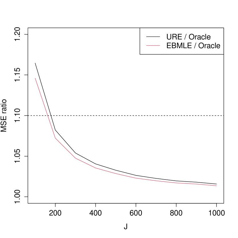
(a) Normal-Normal

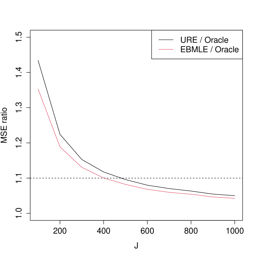
(b) Uniform-Normal

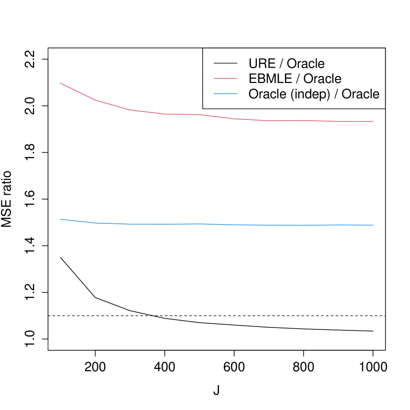
(c) Normal-Normal with group structure

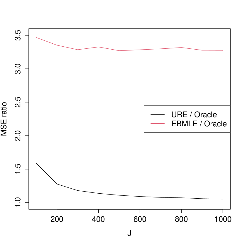
(d) Conditional Heteroskedasticity

Figure 1: Simulation results for the four main scenarios. Each plot has a black line and red lines, which correspond to the MSE of the URE and EBMLE, respectively, as a fraction of the oracle MSE. The x-axis is the sample size from $J=100$ to $1000$. The dotted line is a horizontal line at $1.1$ plotted to see when the MSE of the URE gets within 10% of the oracle.

Figure 1 shows the simulation results for the four main scenarios.In the first Normal-Normal scenario, the true mean vectors are drawn from a normal distribution, $\theta_{j}\overset{\mathrm{i.i.d.}}{\sim}N(0,I_{T})$, the variance matrix from a Wishart distribution, $\Sigma_{j}=\frac{1}{30}\widetilde{\Sigma}_{j}$ where $\widetilde{\Sigma}_{j}\overset{\mathrm{i.i.d.}}{\sim}\mathrm{Wishart}(\Sigma_{0},30)$ with

$$\Sigma_{0}:=\begin{pmatrix}1&.75&.5&.25\\ &1&.75&.5\\ &&1&.75\\ &&&1\end{pmatrix},$$

and $y_{j}\overset{\mathrm{indep}}{\sim}N(\theta_{j},\Sigma_{j}).$ This is a scenario where the distributional assumptions for EB are exactly met. As expected, EBMLE performs well, getting within 10% of the oracle with sample size as small as $J=100$. The URE estimator shows good performance as well, with the difference in MSE with EBMLE being within 2% across all sample sizes.

The DGP of the Uniform-Normal scenario is the same as the Normal-Normal scenario except that $\theta_{jt}{\sim}\mathrm{Unif}[0,.5t]$, drawn independently across both $j$ and $t$. This DGP slightly violates the EB assumptions because the mean parameters are drawn from a uniform distribution rather than a normal distribution, but otherwise satisfies the distributional assumptions imposed by EB. The result is similar to the Normal-Normal case, with the EBMLE performing very well, and the URE estimator showing a very slightly higher MSE than the EBMLE.

The third DGP is similar to the Normal-Normal scenario except that there is a group structure and the mean vectors are serially correlated. Specifically, half of the sample is drawn from the same DGP as in the Normal-Normal scenario, and the remaining half is drawn from a similar Normal-Normal scenario but with higher variance and greater mean. Here, we can think of the DGP as giving a small dependence structure on the mean and variance through the different groups, and thus the EB assumption is violated. Here, the URE estimator still performs well, getting within 10% of the oracle as soon as $J=400$. However, the EBMLE shows MSE significantly higher then the URE, and has about twice the MSE when $J=10^{3}$. The blue line corresponds to the oracle risk when the correlation structure is ignored and thus restricts the hyperprameter space to $\mathcal{L}=\{\mathrm{diag}(\lambda_{1},\dots,\lambda_{4}):\lambda_{t}\geq 0\}$. Ignoring the possible correlation inflates the MSE by around 50%, showing the importance of taking such information into account.

In the last DGP, there are covariates $X_{jt}\in\mathbf{R}^{2}$ drawn from a uniform distribution that affects both $\theta_{j}$ and $\Sigma_{j}$. Hence, here the mean and variance are dependent through the covariates, which again violates the EB assumption. The mean and variance are set as $\theta_{jt}=X^{\prime}_{jt}\beta+U_{jt}$ and $\Sigma_{j}=D_{j}\Sigma_{0}D_{j}$ with $U_{jt}\overset{\mathrm{i.i.d.}}{\sim}\mathrm{Unif}[0,.3]$ and $D_{j}=\mathrm{diag}(X^{\prime}_{j1}\gamma,\dots,X^{\prime}_{jT}\gamma)$. Here, the URE estimator still performs fairly well, with MSE not exceeding the oracle by more than 60% for even smaller sample sizes and getting within 10% of the oracle when $J=600.$ However, the EBMLE shows poor performance. It shows MSE twice as large as the MSE of the URE estimator for $J=100$, and is three times larger for larger $J$. Moreover, if the estimator $\widehat{\theta}^{\mathrm{URE},\mathrm{cov}}$ is used to incorporate the covariates, the risk can be reduced by more than 60% compared to $\widehat{\theta}^{\mathrm{URE},\mathrm{g}}$.

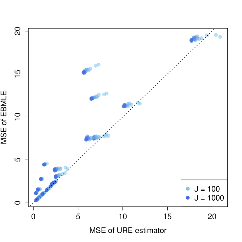
(a) URE vs EBMLE

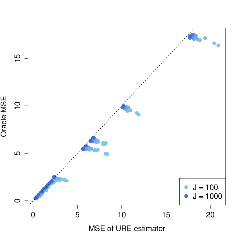
(b) URE vs Oracle

Figure 2: Results from all scenarios. The two plots aggregate the simulation results from all DGPs considered. The left figure is a scatter plot of the MSE of the URE estimator against that of the EBMLE. The color of the dots show the sample size, from $J=100$ to $J=10^{3}$ in increments of $100$, with lighter indicating smaller sample size. The right figure is a scatter plot of the MSE of the URE estimator against the oracle MSE.

Finally, I show two more plots that gather the results from all DGPs I have considered. Figure 2(a) is a scatter plot of the MSE of the URE estimator against the MSE of the EBMLE. The plot shows that while there are some cases where the URE estimator shows slightly higher MSE when the sample size is smaller, the difference vanishes as the sample size gets larger. The majority of the dots lie on top of the 45-degree line, implying that the MSE of the URE estimator is smaller across most scenarios. Figure 2(b) is a similar scatter plot but now the y-axis is the oracle risk rather then the EBMLE risk. By definition of the oracle risk, there can be no dots on top of the 45-degree line. While the lighter blue dots are sometimes a little bit away from the 45-degree line, as the sample size grows larger (i.e., the dots get darker) they get close to the 45-degree line. In particular, all dots that correspond to $J=10^{3}$ are positioned fairly close to the 45-degree line, showing that the MSE of the URE gets close to the oracle across all scenarios.

7 An application to teacher value-added

In this section, I use the proposed methods to estimate the teacher effects on student achievement (i.e., teacher value-added) in the public schools of New York City (NYC). I show that allowing value-added to vary with time and using the URE estimators (and forecasts) give significantly different empirical results compared to the conventional approach.

7.1 Baseline model and data

I use a standard teacher value-added model specified as the following simple linear panel data model introduced in (1):

$$y_{ijt}=X_{ijt}^{\prime}\beta+\alpha_{jt}+\varepsilon_{ijt},$$ (10)

where $y_{ijt}$ is the (standardized) test score in either english language arts (ELA) or math and $X_{ijt}$ is a vector of student characteristics that includes: previous year’s test score, gender, ethnicity, special education status (SWD), english language learner status (ELL), and eligibility for free or reduced price lunch (FL). The results are not sensitive to which covariates are added and/or interacted with other covariates as long as previous year’s test scores are included. The only main difference from the standard models in the literature is the additional $t$ subscript on the teacher fixed effect $\alpha_{jt}$, which allows the teacher fixed effects to vary with time. The idiosyncratic error term $\varepsilon_{ijt}$ is i.i.d. across $i$, $j$, and $t$ with variance $\sigma^{2}$, and is independent with all other times on the right-hand side of (10).

To estimate the value-added model, I use administrative data on all public schools of NYC between academic years 2012/2013 and 2018/2019. The data for the 2012/2013 academic year is used only to extract the information on the students’ test score for the previous year, and thus I have $T=6$. Importantly, the data includes information on, among others, student-teacher linkage. As in Bitler et al. (2019), attention is restricted to 4th and 5th grade students because they are required to take the ELA (and math) test, and it is easy to link a single teacher to each student for elementary school students. I carry out the analysis using ELA test scores, but using the math scores gives similar results. Finally, I restrict the sample to those students whose ELA teachers were present in all six years of the data. The final data includes $J=1,185$ teachers and $174,239$ student-year observations.

Following standard practice in the literature, the coefficient vector is estimated using a fixed effects estimator, with the only difference being the level at which the fixed effects are specified. The signs and magnitudes of each component of the estimate are in line with the results found in the literature (e.g., Koedel et al., 2015 and Bitler et al., 2019). The estimation results are reported in Table 1 of Appendix G.1.

7.2 Some observations from the least squares estimator

The least squares estimator for the fixed effect, $\widehat{\alpha}_{jt}$, is the mean of the residuals corresponding to teacher $j$ and year $t$. I estimate the variance of the least squares estimator by $\widehat{\sigma}^{2}/n_{jt}$ where $\widehat{\sigma}^{2}$ is the usual estimator for the variance term obtained by dividing the sum of squared residuals by the appropriate degrees of freedom, with a precise definition given in Appendix G.1. In the vast majority of the literature, teacher value-added is assumed to be time-invariant, and the least squares estimator for teacher $j$ in this context can be written as $\widehat{\alpha}_{j0}=\frac{1}{n_{j}}\sum_{t=1}^{T}n_{jt}\widehat{\alpha}_{jt}$. I make two preliminary observations regarding the least squares estimators that illustrate 1) there is significant time variation in the fixed effects and that 2) EB methods are unlikely to be optimal in the present setting.

The variation of the least squares estimators within teacher is large, hinting that value-added may vary significantly with time. To see this, I decompose the total variation of the least squares estimator as the variation of within teacher and across teachers:

$$\frac{1}{JT}\sum_{j=1}^{J}\sum_{t=1}^{T}(\widehat{\alpha}_{jt}-\overline{\widehat{\alpha}})^{2}=\frac{1}{J}\sum_{j=1}^{J}\left(\frac{1}{T}\sum_{t=1}^{T}(\widehat{\alpha}_{jt}-\overline{\widehat{\alpha}}_{j.})^{2}\right)+\frac{1}{J}\sum_{j=1}^{J}(\overline{\widehat{\alpha}}_{j.}-\overline{\widehat{\alpha}})^{2}$$ (11)

where $\overline{\widehat{\alpha}}_{j.}:=\frac{1}{T}\sum_{t=1}^{T}\widehat{\alpha}_{jt}$ and $\overline{\widehat{\alpha}}=\frac{1}{JT}\sum_{j=1}^{J}\sum_{t=1}^{T}\widehat{\alpha}_{jt}$ is the average of the least squares estimator at the teacher level and across all teachers, respectively. The first term on the left-hand side can be interpreted as the average variation across time and the second term as the variation across teachers. Calculations show that the average variation across time accounts for about 51% of the total variation. This implies there may be significant time variation in the fixed effects, and thus allowing for the value-added to vary with time can be a more reasonable specification.

The average number of students per teacher in a single year is around $24.5$, with standard deviation approximately as large as $11.7$. This large variation in the number of students per teacher translates to a large degree of heteroskedasticity of the least squares estimators, which is one of the reasons that EB methods can be suboptimal (in frequentist sense). Moreover, an OLS regression of the least squares estimator ($\widehat{\alpha}_{jt}$) on the corresponding cell size ($n_{jt}$) show that there is a significant positive relation between the two variables. This implies that the there may be a dependence structure between the variance of the least squares estimator and the true fixed effect, which is another potential violation of the EB assumptions.

7.3 Estimation results and policy exercise

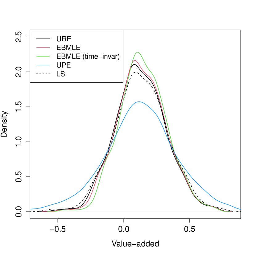
(a) Density plots for shrinkage estimates

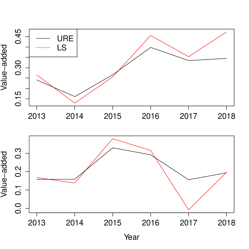
(b) Shrinkage patterns

Figure 3: Shrinkage results. The plot on the left shows the density of the four different estimators discussed. The one on the right shows the time trajectory of the average of value-added estimates for a group of teachers.

Figure 3(a) shows the distribution of teacher value-added estimates using four different estimators: the conventional estimator (EBMLE that assumes that value-added does not vary with time; green), the EBMLE (red) and URE (black) estimators under time-varying value-added, and the optimal UPE forecast (blue) based on the UPE. For the URE and EBMLE estimators under time-varying fixed effects, the average over time within a teacher is used as a summary of the teacher’s value-added, and the density plot is for this average rather than the estimate for each time period. Compared to the least squares estimator (black dashed line), the density of the three estimators excluding the UPE forecast are all more concentrated at the mode, due to the shrinkage. The density plots show that there is a notable difference between the conventional method and the estimators that allow for time drifts. Not allowing for time-varying makes the estimates even more concentrated, and thus the conventional method gives a distribution more concentrated at the mode.

Moreover, the forecasts generated by minimizing the UPE are considerably more disperse than any other estimators. This is expected because unlike the other estimators, there is no averaging step in for the forecasts. Note that under the assumption of the time-invariant fixed effects, the distribution for the forecasts is necessarily the same as the distribution of fixed effect estimates, because there is no difference between a teacher’s current or future fixed effect. However, the significant difference between the blue line and the other lines show that predicting a teacher’s future value-added by only considering past value-added can be misleading.

Figure 3(b) shows how the URE estimator shrinks the least squares estimator. While I use the estimator that shrinks toward a general location, the optimal general location turns out to be close to zero, and thus the URE estimator can be thought to shrink the least squares toward an imaginary horizontal line at zero. As is clear from the plots, the URE estimator does not necessarily shrink each component to zero, but shrinks a smoothed version of the trajectory toward zero. The optimal tuning parameter $\widehat{\Lambda}^{\mathrm{URE}}$ has positive off-diagonal terms, which is in line with positive serial correlation of the true fixed effects. Hence, the estimates for those years with more extreme values gets shrink towards the common trend making the entire trajectory smoother. For example, the least squares estimate for 2016 in the upper plot gets decreased to while that for 2014 gets increased. In contrast, if one does not take into consideration the possible serial correlation, then the URE estimator shrinks the least squares estimator toward zero for each time period, resulting in potential over-shrinkage. This demonstrates the importance of allowing for serial correlation.

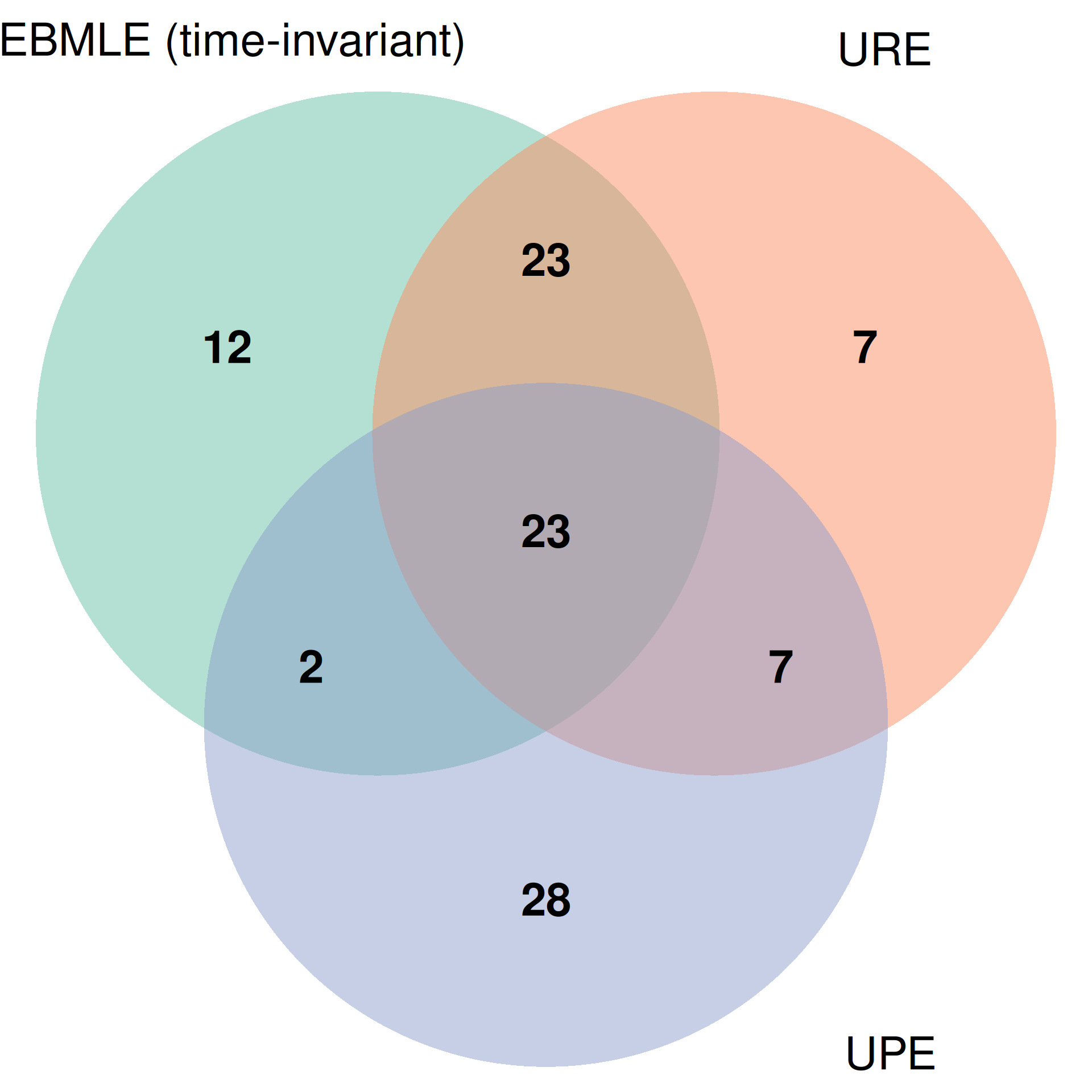
Figure 4: Composition of the bottom 5% teachers under different estimators.

A common policy exercise in the literature (Hanushek, 2011; Chetty et al., 2014b; Gilraine et al., 2020) is to replace the teachers in the bottom 5% in the value-added distribution with an average teacher. I revisit this policy exercise with a focus on how the composition of the bottom 5% teachers changes depending on the choice of the estimator. Figure 4 shows the Venn diagram of the sets of the 60 teachers released under three different choices of estimators: the conventional time-invariant EBMLE, URE, and UPE forecasts. By using the URE estimator instead of the conventional estimator, the composition of the released teachers change by around 24% (14 teachers). Hence, allowing teacher value-added to vary with time significantly changes the composition of the group of teachers to be released. In contrast, Gilraine et al. (2020) find that using a flexible nonparametric EB method (under the assumption of time-invariant value-added) have little effect in the composition of the released teachers. Hence, allowing time drifts indeed seem to be the driving factor of such change.

In policy settings where future performance of the teachers is more relevant than the past performance, it is natural to base the decision on forecasts. For example, if the interest is in maximizing student outcome in the following year, forecasts for the next period teacher value-added is more informative than a summary of past performance. When the value-added is allowed to vary with time, one can use the optimal UPE forecasts in such context. On the other hand, if one specifies value-added to be time-invariant, past and future value-added are the same by definition, and thus will release the bottom 5% according to the conventional estimator. The Venn diagram shows that whether the fixed effects are allowed to vary with time or not changes the composition of the bottom 5% teachers dramatically, with only 25 teachers (approximately 42%) belonging to this group under both estimators.

Under this context, I also consider an out-of-sample exercise that releases the teachers according to different estimators based on the first five years of the data. Then, I calculate the average value-added of the released teachers by taking the least squares estimator corresponding to the sixth year to be the true value-added. Again, the set of teachers released under the two estimators (the conventional one and the forecast) are significantly different, with only a 60% overlap. Importantly, this change in composition is in the right direction: the average value-added of the released teachers is 20% lower when the forecast is used compared to when the conventional estimator is used.

For Online Publication

Appendix A Definition of $\mathcal{M}_{J}$ and $\Gamma_{J}$

The set that $\mu$ is restricted to lie in for the “shrinking to a general location” estimator is defined as

$$\mathcal{M}_{J}:=\{\mu\in\mathbf{R}:\lvert\mu_{t}\rvert\leq q_{1-\tau}(\{\lvert y_{jt}\rvert\}_{j=1}^{J})\,\,\mathrm{for}\,\,t=1,\dots,T\},$$

where $q_{1-\tau}(\{\lvert y_{jt}\rvert\}_{j=1}^{J})$ denotes the $1-\tau$ sample quantile of $\{\lvert y_{jt}\rvert\}_{j=1}^{J}$. I recommend choosing a small $\tau$, such as $\tau=.01$. This restricts the centering term, component-wise, to be somewhere smaller than the 99 percentile of the data in terms of magnitude. I argue that this restriction is reasonable, because it seems rather hard to justify shrinking the data toward a point where there are almost no observations. In fact, this constraint is never binding in any of the simulation iterations reported in Section 6.

The set that $\gamma$ is restricted to lie in for the “shrinking to a linear combination of covariates” estimator is defined as

$$\Gamma_{J}:=\{\gamma\in\mathbf{R}^{k}:\lVert\gamma\rVert\leq B\lVert\widehat{\gamma}^{\mathrm{OLS}}\rVert\},$$

where $B$ is a large constant that does not depend on $J$, and $\widehat{\gamma}^{\mathrm{OLS}}$ is the pooled OLS estimator obtained by regressing $y_{j}$ on $X_{j}$, i.e., $\widehat{\gamma}^{\mathrm{OLS}}=(\sum_{j=1}^{J}Z_{j}^{\prime}Z_{j})^{-1}\sum_{j=1}^{J}Z_{j}^{\prime}y_{j}$. The idea is to include the intuitive OLS, and potentially coefficients with much larger magnitude as well. In simulations, I use $B=10^{3}$ and this constraint never binds.

Appendix B Proof of main theorems

B.1 Proof of Theorem 4.1

The difference between the URE and the loss is given as

$$\mathrm{URE}(\mu,\Lambda)-\ell(\theta,\widehat{\theta}(\mu,\Lambda))$$

$$= \frac{1}{J}\sum_{j=1}^{J}\left(\mathrm{URE}_{j}(\mu,\Lambda)-(\widehat{\theta}_{j}(\mu,\Lambda)-\theta_{j})^{\prime}(\widehat{\theta}_{j}(\mu,\Lambda)-\theta_{j})\right).$$

Expanding the summand of the second line gives

$$\begin{aligned} &\mathrm{URE}_{j}(\mu,\Lambda)-(\widehat{\theta}_{j}(\mu,\Lambda)-\theta_{j})^{\prime}(\widehat{\theta}_{j}(\mu,\Lambda)-\theta_{j})\\ =&\operatorname{\mathrm{tr}}(\Sigma_{j})-2\operatorname{\mathrm{tr}}((\Lambda+\Sigma_{j})^{-1}\Sigma_{j}^{2})\\ &+(y_{j}-\mu)^{\prime}[(\Lambda+\Sigma_{j})^{-1}\Sigma_{j}^{2}(\Lambda+\Sigma_{j})^{-1}](y_{j}-\mu)\\ &-(y_{j}-\theta_{j}-\Sigma_{j}(\Lambda+\Sigma_{j})^{-1}(y_{j}-\mu))^{\prime}(y_{j}-\theta_{j}-\Sigma_{j}(\Lambda+\Sigma_{j})^{-1}(y_{j}-\mu))\\ =&\operatorname{\mathrm{tr}}(\Sigma_{j})-2\operatorname{\mathrm{tr}}((\Lambda+\Sigma_{j})^{-1}\Sigma_{j}^{2})-(y_{j}-\theta_{j})^{\prime}(y_{j}-\theta_{j})\\ &+2(y_{j}-\mu)^{\prime}(\Lambda+\Sigma_{j})^{-1}\Sigma_{j}(y_{j}-\theta_{j})\\ =&y_{j}^{\prime}y_{j}-\theta_{j}^{\prime}\theta_{j}-\operatorname{\mathrm{tr}}(\Sigma_{j})-2\operatorname{\mathrm{tr}}(\Lambda(\Lambda+\Sigma_{j})^{-1}(y_{j}y_{j}^{\prime}-y_{j}\theta_{j}^{\prime}-\Sigma_{j}))\\ &-2\mu^{\prime}(\Lambda+\Sigma_{j})^{-1}\Sigma_{j}(y_{j}-\theta_{j}).\end{aligned}$$ (12)

Taking $\mu=0$, I obtain

$$\begin{aligned} &\mathrm{URE}_{j}(\Lambda)-(\widehat{\theta}_{j}(\Lambda)-\theta_{j})^{\prime}(\widehat{\theta}_{j}(\Lambda)-\theta_{j})\\ =&y_{j}^{\prime}y_{j}-\theta_{j}^{\prime}\theta_{j}-\operatorname{\mathrm{tr}}(\Sigma_{j})-2\operatorname{\mathrm{tr}}(\Lambda(\Lambda+\Sigma_{j})^{-1}(y_{j}y_{j}^{\prime}-y_{j}\theta_{j}^{\prime}-\Sigma_{j})),\end{aligned}$$

where, for simplicity, I write $\mathrm{URE}_{j}(\Lambda)$ as a shorthand for $\mathrm{URE}_{j}(0,\Lambda)$, and likewise for $\mathrm{URE}(\Lambda)$ and $\widehat{\theta}(\Lambda)$. It follows that

$$\sup_{\Lambda}\left\lvert\mathrm{URE}(\Lambda)-\ell(\theta,\widehat{\theta}(\Lambda))\right\rvert= \sup_{\Lambda}\left\lvert\frac{1}{J}\sum\nolimits_{j=1}^{J}(\mathrm{URE}_{j}(\Lambda)-\ell_{j}(\theta_{j},\widehat{\theta}_{j}(\Lambda)))\right\rvert$$

$$\leq \left\lvert\frac{1}{J}\sum\nolimits_{j=1}^{J}(y_{j}^{\prime}y_{j}-\theta_{j}^{\prime}\theta_{j}-\operatorname{\mathrm{tr}}(\Sigma_{j}))\right\rvert$$

$$+\sup_{\Lambda}\left\lvert\frac{1}{J}\sum\nolimits_{j=1}^{J}\operatorname{\mathrm{tr}}(\Lambda(\Lambda+\Sigma_{j})^{-1}(y_{j}y_{j}^{\prime}-y_{j}\theta_{j}^{\prime}-\Sigma_{j}))\right\rvert,$$

where the inequality follows from the triangle inequality. I show that each of the two terms in the last expression converges to zero in $L^{1}$.

For the first term, because $\operatorname{\mathbf{E}}y_{j}^{\prime}y_{j}=\theta_{j}^{\prime}\theta_{j}+\operatorname{\mathrm{tr}}(\Sigma_{j})$ for all $j\leq J$ and $y_{j}$’s are independent, I have

$$\operatorname{\mathbf{E}}\left(\frac{1}{J}\sum_{j=1}^{J}(y_{j}^{\prime}y_{j}-\theta_{j}^{\prime}\theta_{j}-\operatorname{\mathrm{tr}}(\Sigma_{j}))\right)^{2} =\frac{1}{J^{2}}\sum_{j=1}^{J}\operatorname{\mathbf{E}}(y_{j}^{\prime}y_{j}-\theta_{j}^{\prime}\theta_{j}-\operatorname{\mathrm{tr}}(\Sigma_{j}))^{2}$$

$$=\frac{1}{J^{2}}\sum_{j=1}^{J}\operatorname{\mathrm{var}}(y_{j}^{\prime}y_{j}).$$

Therefore, if $\lim\frac{1}{J^{2}}\sum_{j=1}^{J}\operatorname{\mathrm{var}}(y_{j}^{\prime}y_{j})=0$, then this term converges to zero in $L^{2}$ and thus in $L^{1}$. Assumption 4.1(ii) ensures that this is the case.

For the second term, note that

$$\sup_{\Lambda}\left\lvert\frac{1}{J}\sum_{j=1}^{J}\operatorname{\mathrm{tr}}(\Lambda(\Lambda+\Sigma_{j})^{-1}(y_{j}y_{j}^{\prime}-y_{j}\theta_{j}^{\prime}-\Sigma_{j}))\right\rvert$$

$$= \sup_{\Lambda}\left\lvert\frac{1}{J}\sum_{j=1}^{J}\operatorname{\mathrm{tr}}((I-\Sigma_{j}(\Lambda+\Sigma_{j})^{-1})(y_{j}y_{j}^{\prime}-y_{j}\theta_{j}^{\prime}-\Sigma_{j}))\right\rvert$$

$$\leq \left\lvert\frac{1}{J}\sum_{j=1}^{J}(y_{j}^{\prime}y_{j}-\theta_{j}^{\prime}y_{j}-\operatorname{\mathrm{tr}}(\Sigma_{j}))\right\rvert+\sup_{\Lambda}\left\lvert\frac{1}{J}\sum_{j=1}^{J}\operatorname{\mathrm{tr}}(\Sigma_{j}(\Lambda+\Sigma_{j})^{-1}(y_{j}y_{j}^{\prime}-y_{j}\theta_{j}^{\prime}-\Sigma_{j}))\right\rvert$$

$$= :\mathrm{(I)}_{J}+\mathrm{(II)}_{J}.$$

To show that $\mathrm{(I)}_{J}\overset{L^{1}}{\to}0$, I again show $L^{2}$ convergence. Because $\operatorname{\mathbf{E}}(y_{j}^{\prime}y_{j}-\theta_{j}^{\prime}y_{j})=\operatorname{\mathrm{tr}}(\Sigma_{j})$ for all $j\leq J$ and $y_{j}$’s are independent, it follows that

$$\operatorname{\mathbf{E}}\left(\frac{1}{J}\sum_{j=1}^{J}(y_{j}^{\prime}y_{j}-\theta_{j}^{\prime}y_{j}-\operatorname{\mathrm{tr}}(\Sigma_{j}))\right)^{2}= \frac{1}{J^{2}}\sum_{j=1}^{J}\operatorname{\mathbf{E}}(y_{j}^{\prime}y_{j}-\theta_{j}^{\prime}y_{j}-\operatorname{\mathrm{tr}}(\Sigma_{j}))^{2}$$

$$= \frac{1}{J^{2}}\sum_{j=1}^{J}\operatorname{\mathrm{var}}(y_{j}^{\prime}y_{j}-\theta_{j}^{\prime}y_{j}).$$

Hence, it suffices to establish that $\lim_{J\to\infty}\frac{1}{J^{2}}\sum_{j=1}^{J}\operatorname{\mathrm{var}}(y_{j}^{\prime}y_{j}-\theta_{j}^{\prime}y_{j})=0$. The summand is bounded by

$$\operatorname{\mathrm{var}}(y_{j}^{\prime}y_{j}-\theta_{j}^{\prime}y_{j})\leq 2\operatorname{\mathrm{var}}(y_{j}^{\prime}y_{j})+2\theta_{j}^{\prime}\Sigma_{j}\theta_{j}\leq 2\operatorname{\mathrm{var}}(y_{j}^{\prime}y_{j})+2\operatorname{\mathrm{tr}}(\Sigma_{j})\lVert\theta_{j}\rVert_{\infty}^{2}.$$

Hence, if ${\lim\sup}_{J\to\infty}\frac{1}{J}\sum_{j=1}^{J}(\operatorname{\mathrm{var}}(y_{j}^{\prime}y_{j})+\operatorname{\mathrm{tr}}(\Sigma_{j})\lVert\theta_{j}\rVert_{\infty}^{2})<\infty$ it follows that $\mathrm{(I)}_{J}\overset{L^{2}}{\to}0.$ A sufficient condition for this to hold is that $\sup_{j}\operatorname{\mathrm{var}}(y_{j}^{\prime}y_{j})$, $\sup_{j}\operatorname{\mathrm{tr}}(\Sigma_{j})$, and $\sup_{j}\lVert\theta_{j}\rVert_{\infty}^{2}$ are all finite, which is true by Assumption 4.1 (ii).

To show that $\mathrm{(II)}_{J}\overset{L^{1}}{\to}0$, define the random function ${G}_{J}(\Lambda)$ as

$${G}_{J}(\Lambda)=\frac{1}{J}\sum_{j=1}^{J}\operatorname{\mathrm{tr}}(\Sigma_{j}(\Lambda+\Sigma_{j})^{-1}(y_{j}y_{j}^{\prime}-y_{j}\theta_{j}^{\prime}-\Sigma_{j}))$$

so that the aim is to show $\sup_{\Lambda}\lvert{G}_{J}(\Lambda)\rvert\overset{L^{1}}{\to}0.$ I use the fact that convergence in probability and a uniform integrability condition imply convergence in $L^{1}$. That is, I show $\sup_{\Lambda}\lvert{G}_{J}(\Lambda)\rvert\overset{p}{\to}0$ and that $\left\{\sup_{\Lambda}\lvert{G}_{J}(\Lambda)\rvert\right\}_{J\geq 1}$ is uniformly integrable.

I show $\sup_{\Lambda}\lvert{G}_{J}(\Lambda)\rvert\overset{p}{\to}0$ by using the results given by Andrews (1992).The results therein require a totally bounded parameter space. However, the parameter space in consideration, $\mathcal{S}_{T}^{+}$, does not satisfy this requirement. This can be dealt with by an appropriate reparametrization. Let $\underline{\sigma}_{\Sigma}=\inf_{j}\sigma_{T}(\Sigma_{j})$ denote the infimum of the smallest eigenvalues of $\Sigma_{j}$’s for $j\geq 1$, which is bounded away from zero by assumption. Consider the transformation defined by $h(\Lambda)=(\underline{\sigma}_{\Sigma}I_{T}+\Lambda)^{-1}$, and write the image of such transformation as $\widetilde{\mathcal{L}}:=\{h(\Lambda):\Lambda\in S^{+}_{T}\}$. Note that $h:\mathcal{S}_{T}^{+}\to\widetilde{\mathcal{L}}$ is one-to-one and onto, with its inverse given as $h^{-1}(\widetilde{\Lambda})=\widetilde{\Lambda}^{-1}-\underline{\sigma}_{\Sigma}I_{T}.$ For $\widetilde{\Lambda}\in\widetilde{\mathcal{L}}$, define $\widetilde{G}_{J}:=G_{J}\circ h^{-1}$ so that

$$\sup_{\Lambda\in\mathcal{S}_{T}^{+}}\lvert{G}_{J}(\Lambda)\rvert=\sup_{\Lambda\in\mathcal{S}_{T}^{+}}\lvert{G}_{J}(h^{-1}(h(\Lambda)))\rvert=\sup_{\widetilde{\Lambda}\in\widetilde{\mathcal{L}}}\lvert{G}_{J}(h^{-1}(\widetilde{\Lambda}))\rvert=\sup_{\widetilde{\Lambda}\in\widetilde{\mathcal{L}}}\lvert\widetilde{G}_{J}(\widetilde{\Lambda})\rvert.$$

Hence, showing $\sup_{\Lambda}\lvert{G}_{J}(\Lambda)\rvert\overset{p}{\to}0$ is equivalent to $\sup_{\widetilde{\Lambda}\in\widetilde{\mathcal{L}}}\lvert\widetilde{G}_{J}(\widetilde{\Lambda})\rvert\overset{p}{\to}0.$ Let $\mathcal{S}_{T}$ denote the set of all real positive $T\times T$ matrices. While the choice of metric is irrelevant, equip $\mathcal{S}_{T}$ with the metric $d$ induced by the Frobenius norm for concreteness. Note that $\widetilde{\mathcal{L}}\subset S_{T}$. I show that the (reparametrized) parameter space $\widetilde{\mathcal{L}}$ is indeed totally bounded. For any $\widetilde{\Lambda}\in\widetilde{\mathcal{L}}$, I have $0\leq\widetilde{\Lambda}\leq\underline{\sigma}_{\Sigma}^{-1}I_{T}$ so that $\sigma_{1}(\widetilde{\Lambda})\leq\underline{\sigma}_{\Sigma}^{-1}$. Moreover, since the largest singular value equals the operator norm and all norms on $S_{T}$ are equivalent, this shows that $\widetilde{\mathcal{L}}$ is bounded, and thus totally bounded because $\widetilde{\mathcal{L}}$ can be seen as a subset of the Euclidean space with dimension $T^{2}$.

It remains to show that a) $\lvert\widetilde{G}_{J}(\widetilde{\Lambda})\rvert\overset{p}{\to}0$ for all $\widetilde{\Lambda}\in\widetilde{\mathcal{L}}$ and b) $\widetilde{G}_{J}(\widetilde{\Lambda})$ is stochastically equicontinuous. For a), I can show $\lvert G_{J}(\Lambda)\rvert\overset{p}{\to}0$ for all $\Lambda\in\mathcal{S}_{T}^{+}$ instead because for any $\widetilde{\Lambda}\in\widetilde{\mathcal{L}}$, there exists $\Lambda\in\mathcal{S}_{T}^{+}$ such that $G_{J}(\Lambda)=\widetilde{G}_{J}(\widetilde{\Lambda})$. Now, note that

$$\,\operatorname{\mathbf{E}}\operatorname{\mathrm{tr}}(\Sigma_{j}(\Lambda+\Sigma_{j})^{-1}(y_{j}y_{j}^{\prime}-y_{j}\theta_{j}^{\prime}-\Sigma_{j}))$$

$$= \,\operatorname{\mathrm{tr}}(\Sigma_{j}(\Lambda+\Sigma_{j})^{-1}\operatorname{\mathbf{E}}(y_{j}y_{j}^{\prime}-y_{j}\theta_{j}^{\prime}-\Sigma_{j}))=0,$$

and $y_{j}$’s are independent. This gives

$$\operatorname{\mathbf{E}}G_{J}(\Lambda)^{2}=\frac{1}{J^{2}}\sum_{j=1}^{J}\operatorname{\mathbf{E}}\operatorname{\mathrm{tr}}(\Sigma_{j}(\Lambda+\Sigma_{j})^{-1}(y_{j}y_{j}^{\prime}-y_{j}\theta_{j}^{\prime}-\Sigma_{j}))^{2}$$

I give a bound on $\lvert\operatorname{\mathrm{tr}}(\Sigma_{j}(\Lambda+\Sigma_{j})^{-1}(y_{j}y_{j}^{\prime}-y_{j}\theta_{j}^{\prime}-\Sigma_{j}))\rvert.$ Let $UDU^{\prime}$ denote the spectral decomposition of $\Sigma_{j}^{-1/2}\Lambda\Sigma_{j}^{-1/2}$ with $D=\mathrm{diag}(d_{1},\dots,d_{T})$. Then, I have

$$\Sigma_{j}(\Lambda+\Sigma_{j})^{-1}=\Sigma_{j}^{1/2}U(I_{T}+D)^{-1}U^{\prime}\Sigma_{j}^{-1/2}.$$

It follows that

$$\begin{aligned} &\operatorname{\mathrm{tr}}(\Sigma_{j}(\Lambda+\Sigma_{j})^{-1}(y_{j}y_{j}^{\prime}-y_{j}\theta_{j}^{\prime}-\Sigma_{j}))\\ =&\operatorname{\mathrm{tr}}(\Sigma_{j}^{1/2}U(I_{T}+D)^{-1}U^{\prime}\Sigma_{j}^{-1/2}(y_{j}y_{j}^{\prime}-y_{j}\theta_{j}^{\prime}-\Sigma_{j}))\\ =&\operatorname{\mathrm{tr}}((I_{T}+D)^{-1}U^{\prime}\Sigma_{j}^{-1/2}(y_{j}y_{j}^{\prime}-\theta_{j}y_{j}^{\prime}-\Sigma_{j})\Sigma_{j}^{1/2}U).\end{aligned}$$ (13)

Write $H_{j}=\Sigma_{j}^{-1/2}(y_{j}y_{j}^{\prime}-y_{j}\theta_{j}^{\prime}-\Sigma_{j})\Sigma_{j}^{1/2}$, and observe that

$$\begin{aligned} &\left\lvert\operatorname{\mathrm{tr}}((I_{T}+D)^{-1}U^{\prime}\Sigma_{j}^{-1/2}(y_{j}y_{j}^{\prime}-y_{j}\theta_{j}^{\prime}-\Sigma_{j})\Sigma_{j}^{1/2}U)\right\rvert\\ =&\left\lvert\sum_{t=1}^{T}\frac{1}{1+d_{t}}(U^{\prime}H_{j}U)_{tt}\right\rvert\\ \leq&\sum_{t=1}^{T}\frac{1}{1+d_{t}}\left\lvert(U^{\prime}H_{j}U)_{tt}\right\rvert\\ \leq&\sum_{t=1}^{T}\left\lvert(U^{\prime}H_{j}U)_{tt}\right\rvert,\end{aligned}$$ (14)

where the last inequality holds because $0\leq 1/(1+d_{t})\leq 1$. Let $U_{t}$ denote the $t$th column of the orthogonal matrix $U$. I have

$$\left\lvert(U^{\prime}H_{j}U)_{tt}\right\rvert=\left\lvert U_{t}^{\prime}H_{j}U_{t}\right\rvert\leq\left\lVert H_{j}U_{t}\right\rVert\leq\sup_{U\in\mathbb{R}^{T},\lVert U\rVert=1}\lVert H_{j}U\rVert=\sigma_{1}(H_{j}),$$

where the first inequality follows from Cauchy-Schwarz, and the last equality from the fact that the operator norm of a matrix is equal to its largest singular value.

Combining these results gives

$$\operatorname{\mathbf{E}}G_{J}(\Lambda)^{2}\leq\frac{T^{2}}{J^{2}}\sum_{j=1}^{J}\operatorname{\mathbf{E}}\,\sigma_{1}(H_{j})^{2}.$$

Now, to derive a bound for $\sigma_{1}(H_{j})$, observe that

$$\sigma_{1}(H_{j})= \sigma_{1}(\Sigma_{j}^{-1/2}(y_{j}y_{j}^{\prime}-y_{j}\theta_{j}^{\prime}-\Sigma_{j})\Sigma_{j}^{1/2})$$

$$\leq \sigma_{1}(\Sigma_{j}^{-1/2})\sigma_{1}(y_{j}y_{j}^{\prime}-y_{j}\theta_{j}^{\prime}-\Sigma_{j})\sigma_{1}(\Sigma_{j}^{1/2})$$

$$\leq \kappa(\Sigma_{j})^{1/2}\sigma_{1}(y_{j}y_{j}^{\prime}-y_{j}\theta_{j}^{\prime}-\Sigma_{j}).$$

Since the largest singular value of a matrix is bounded by its Frobenius norm, it follows that

$$\sigma_{1}(y_{j}y_{j}^{\prime}-y_{j}\theta_{j}^{\prime}-\Sigma_{j})^{2}$$

$$\leq \operatorname{\mathrm{tr}}((y_{j}y_{j}^{\prime}-y_{j}\theta_{j}^{\prime}-\Sigma_{j})^{\prime}(y_{j}y_{j}^{\prime}-y_{j}\theta_{j}^{\prime}-\Sigma_{j}))$$

$$= (y_{j}^{\prime}y_{j})^{2}+\theta_{j}^{\prime}y_{j}\theta_{j}^{\prime}y_{j}+\sigma^{4}\operatorname{\mathrm{tr}}(\Sigma_{j})^{2}-2y_{j}^{\prime}y_{j}y_{j}^{\prime}\theta_{j}-2y^{\prime}_{j}\Sigma_{j}y_{j}+2\theta_{j}^{\prime}\Sigma_{j}y_{j}.$$

Taking expectations yields

$$\operatorname{\mathbf{E}}(y_{j}^{\prime}y_{j})^{2}+\theta_{j}^{\prime}\theta_{j}\operatorname{\mathbf{E}}y_{j}^{\prime}y_{j}+\sigma^{4}\operatorname{\mathrm{tr}}(\Sigma_{j})^{2}-2\operatorname{\mathbf{E}}y_{j}^{\prime}y_{j}y_{j}^{\prime}\theta_{j}-2\operatorname{\mathbf{E}}y^{\prime}_{j}\Sigma_{j}y_{j}+2\theta_{j}^{\prime}\Sigma_{j}\operatorname{\mathbf{E}}y_{j}$$

$$= \operatorname{\mathrm{var}}(y_{j}^{\prime}y_{j})+(\theta_{j}^{\prime}\theta_{j}+\operatorname{\mathrm{tr}}(\Sigma_{j}))^{2}+\theta_{j}^{\prime}\theta_{j}(\theta_{j}^{\prime}\theta_{j}+\operatorname{\mathrm{tr}}(\Sigma_{j}))$$

$$+\sigma^{4}\operatorname{\mathrm{tr}}(\Sigma_{j})^{2}-2\theta_{j}^{\prime}\operatorname{\mathbf{E}}(y_{j}y_{j}^{\prime}y_{j})-2\theta_{j}^{\prime}\Sigma_{j}\theta_{j}-2\sigma^{4}\operatorname{\mathrm{tr}}(\Sigma_{j})^{2}+2\theta_{j}^{\prime}\Sigma_{j}\theta_{j}$$

$$= \operatorname{\mathrm{var}}(y_{j}^{\prime}y_{j})+2(\theta_{j}^{\prime}\theta_{j})^{2}+3\theta_{j}^{\prime}\theta_{j}\operatorname{\mathrm{tr}}(\Sigma_{j})-2\theta_{j}^{\prime}\operatorname{\mathbf{E}}(y_{j}y_{j}^{\prime}y_{j})$$

$$\leq \operatorname{\mathrm{var}}(y_{j}^{\prime}y_{j})+2\lVert\theta_{j}\rVert^{4}+3\lVert\theta_{j}\rVert^{2}\operatorname{\mathrm{tr}}(\Sigma_{j})+2\lVert\theta_{j}\rVert\operatorname{\mathbf{E}}\lVert y_{j}\rVert^{3}.$$

This shows that if

$$\underset{J\to\infty}{\lim\sup}\frac{1}{J}\sum_{j=1}^{J}\kappa(\Sigma_{j})\left(\operatorname{\mathrm{var}}(y_{j}^{\prime}y_{j})+2\lVert\theta_{j}\rVert^{4}+3\lVert\theta_{j}\rVert^{2}\operatorname{\mathrm{tr}}(\Sigma_{j})+2\lVert\theta_{j}\rVert\operatorname{\mathbf{E}}(\lVert y_{j}\rVert^{3})\right)<\infty,$$ (15)

then $\lvert G_{J}(\Lambda)\rvert\to 0$ in $L^{2}$, and thus in probability. Hence, if $\sup_{j}\sigma_{1}(\Sigma_{j})/\sigma_{T}(\Sigma_{j})$, $\sup_{j}\operatorname{\mathrm{var}}(y_{j}^{\prime}y_{j})$, $\sup_{j}\lvert\theta_{j}\rvert$, and $\sup_{j}\operatorname{\mathrm{tr}}(\Sigma_{j})$ are bounded, the result holds. Note that this true by Assumption 4.1.

It remains to show that $\widetilde{G}_{J}(\widetilde{\Lambda})$ is stochastically equicontinuous. I do this by showing that $\widetilde{G}_{J}(\widetilde{\Lambda})$ satisfies a Lipschitz condition as in Assumption SE-1 of Andrews (1992). Specifically, I show that $\lvert\widetilde{G}_{J}(\widetilde{\Lambda})-\widetilde{G}_{J}(\widetilde{\Lambda}^{\dagger})\rvert\leq B_{J}\lVert\widetilde{\Lambda}-\widetilde{\Lambda}^{\dagger}\rVert$ for all $\widetilde{\Lambda},\widetilde{\Lambda}^{\dagger}\in\widetilde{\mathcal{L}}$ with $B_{J}=O_{p}(1)$. Let $\widetilde{\Lambda},\widetilde{\Lambda}^{\dagger}\in\widetilde{\mathcal{L}}$ be arbitrarily taken. First, I show that $\widetilde{\mathcal{L}}$ is convex. Take any $\alpha\in[0,1]$. Note that $\alpha\widetilde{\Lambda}+(1-\alpha)\widetilde{\Lambda}^{\dagger}$ is nonsingular because $\widetilde{\Lambda}$ and $\widetilde{\Lambda}^{\dagger}$ are positive definite and the space of positive definite matrices is convex. Then, for $\Lambda_{\alpha}=(\alpha\widetilde{\Lambda}+(1-\alpha)\widetilde{\Lambda}^{\dagger})^{-1}-\underline{\sigma}_{\Sigma}I_{T}$, I have $h(\Lambda_{\alpha})=\alpha\widetilde{\Lambda}+(1-\alpha)\widetilde{\Lambda}^{\dagger},$ which shows that $\alpha\widetilde{\Lambda}+(1-\alpha)\widetilde{\Lambda}^{\dagger}\in\widetilde{\mathcal{L}}$. The mean value theorem gives

$$\widetilde{G}_{J}(\widetilde{\Lambda})-\widetilde{G}_{J}(\widetilde{\Lambda}^{\dagger})=\nabla\widetilde{G}_{J}(\widetilde{\Lambda}^{\alpha})\cdot\mathrm{vec}(\widetilde{\Lambda}-\widetilde{\Lambda}^{\dagger}),$$

where $\nabla\widetilde{G}_{J}(\widetilde{\Lambda}):=\frac{\partial}{\partial\mathrm{vec}(\widetilde{\Lambda})}\widetilde{G}_{J}(\widetilde{\Lambda})$, and $\widetilde{\Lambda}^{\alpha}:=\alpha\widetilde{\Lambda}+(1-\alpha)\widetilde{\Lambda}^{\dagger}$ for some $\alpha\in[0,1]$. This implies, by Cauchy-Schwarz,

$$\lvert\widetilde{G}_{J}(\widetilde{\Lambda})-\widetilde{G}_{J}(\widetilde{\Lambda}^{\dagger})\rvert\leq\lVert\nabla\widetilde{G}_{J}(\widetilde{\Lambda}^{\alpha})\rVert\lVert\widetilde{\Lambda}-\widetilde{\Lambda}^{\dagger}\rVert,$$ (16)

where I use the fact that the Frobenius norm of a matrix and the Euclidean norm of the vectorized version of it are the same. Note that $\lVert\nabla\widetilde{G}_{J}(\widetilde{\Lambda})\rVert=\lVert\frac{\partial}{\partial\widetilde{\Lambda}}\widetilde{G}_{J}(\widetilde{\Lambda})\rVert$ by definition of the Frobenius norm.

By the formula for the derivative of a matrix inverse and the derivative of a trace, and the chain rule for matrix derivatives, I have

$$\frac{\partial}{\partial\widetilde{\Lambda}}G_{J}(\widetilde{\Lambda})$$

$$= \frac{1}{J}\sum_{j=1}^{J}\widetilde{\Lambda}^{-1}(\widetilde{\Lambda}^{-1}-\underline{\sigma}_{\Sigma}I_{T}+\Sigma_{j})^{-1}\Sigma_{j}(y_{j}y_{j}^{\prime}-y_{j}\theta_{j}^{\prime}-\Sigma_{j})(\widetilde{\Lambda}^{-1}-\underline{\sigma}_{\Sigma}I_{T}+\Sigma_{j})^{-1}\widetilde{\Lambda}^{-1}.$$

Write the summand in the second line as $g_{j}(\widetilde{\Lambda})$. I first derive a bound on $\sigma_{1}(g_{j}(\widetilde{\Lambda}))$, and use this to bound $\lVert\textstyle\frac{\partial}{\partial\widetilde{\Lambda}}G_{J}(\widetilde{\Lambda})\rVert$ by using the fact that

$$\left\lVert\frac{\partial}{\partial\widetilde{\Lambda}}G_{J}(\widetilde{\Lambda})\right\rVert\leq T^{1/2}\sigma_{1}\left(\frac{\partial}{\partial\widetilde{\Lambda}}G_{J}(\widetilde{\Lambda})\right)\leq\frac{1}{J}\sum_{j=1}^{J}\sigma_{1}(g_{j}(\widetilde{\Lambda})).$$

Since the operator norm is submultiplicative, it follows that

$$\sigma_{1}(g_{j}(\widetilde{\Lambda}))\leq\sigma_{1}(\widetilde{\Lambda}^{-1}(\widetilde{\Lambda}^{-1}-\underline{\sigma}_{\Sigma}I_{T}+\Sigma_{j})^{-1})^{2}\sigma_{1}(\Sigma_{j}(y_{j}y_{j}^{\prime}-y_{j}\theta_{j}^{\prime}-\Sigma_{j})).$$

I proceed by bounding the two singular values that appear on the right hand side. For the first term, note that

$$\begin{aligned} &\sigma_{1}(\widetilde{\Lambda}^{-1}(\widetilde{\Lambda}^{-1}-\underline{\sigma}_{\Sigma}I_{T}+\Sigma_{j})^{-1})^{2}\\ =&\sigma_{1}(\widetilde{\Lambda}^{-1}(\widetilde{\Lambda}^{-1}-\underline{\sigma}_{\Sigma}I_{T}+\Sigma_{j})^{-2}\widetilde{\Lambda}^{-1})\\ =&\sigma_{1}((I+\widetilde{\Lambda}^{1/2}(\Sigma_{j}-\underline{\sigma}_{\Sigma}I_{T})\widetilde{\Lambda}^{1/2})^{-2})\\ \leq&1,\end{aligned}$$ (17)

where the first equality uses the fact that $\sigma_{1}(A)^{2}=\sigma_{1}(AA^{\prime})=\sigma_{1}(A^{\prime}A)$ for any matrix $A$. The last inequality follows because $\widetilde{\Lambda}^{1/2}(\Sigma_{j}-\underline{\sigma}_{\Sigma}I_{T})\widetilde{\Lambda}^{1/2}$ is positive semidefinite so that $0\leq(I+\widetilde{\Lambda}^{1/2}(\Sigma_{j}-\underline{\sigma}_{\Sigma}I_{T})\widetilde{\Lambda}^{1/2})^{-2}\leq I_{T}$, and $A\leq B$ implies $\sigma_{1}(A)\leq\sigma_{1}(B)$ for any two positive semidefinite matrices $A$ and $B$. A bound on $\sigma_{1}(\Sigma_{j}(y_{j}y_{j}^{\prime}-y_{j}\theta_{j}^{\prime}-\Sigma_{j}))$ is given by

$$\sigma_{1}(\Sigma_{j}(y_{j}y_{j}^{\prime}-y_{j}\theta_{j}^{\prime}-\Sigma_{j}))\leq\sigma_{1}(\Sigma_{j})(y_{j}^{\prime}y_{j}+(y_{j}^{\prime}y_{j})^{1/2}(\theta_{j}^{\prime}\theta_{j})^{1/2}+\sigma_{1}(\Sigma_{j})).$$

Combining these results, I obtain

$$\sup_{\widetilde{\Lambda}\in\widetilde{\mathcal{L}}}\,\left\lVert\frac{\partial}{\partial\widetilde{\Lambda}}G_{J}(\widetilde{\Lambda})\right\rVert\leq \frac{1}{J}\sum_{j=1}^{J}\sigma_{1}(\Sigma_{j})(y_{j}^{\prime}y_{j}+\lVert y_{j}\rVert\lVert\theta_{j}\rVert+\sigma_{1}(\Sigma_{j}))$$

$$= \frac{1}{J}\sum_{j=1}^{J}\sigma_{1}(\Sigma_{j})\left(y_{j}^{\prime}y_{j}+\lVert y_{j}\rVert\lVert\theta_{j}\rVert-\operatorname{\mathbf{E}}(y_{j}^{\prime}y_{j}+\lVert y_{j}\rVert\lVert\theta_{j}\rVert)\right)$$

$$+\frac{1}{J}\sum_{j=1}^{J}\left(\operatorname{\mathbf{E}}(y_{j}^{\prime}y_{j}+\lVert y_{j}\rVert\lVert\theta_{j}\rVert)+\sigma_{1}(\Sigma_{j})\right).$$

The term in the second line is $o_{p}(1)$ because

$$\textstyle\sup_{j}\operatorname{\mathrm{var}}(\sigma_{1}(\Sigma_{j})(y_{j}^{\prime}y_{j}+\lVert y_{j}\rVert\lVert\theta_{j}\rVert))\leq 2\textstyle\sup_{j}\sigma_{1}^{2}(\Sigma_{j})(\operatorname{\mathbf{E}}\lVert y_{j}\rVert^{4}+\lVert\theta_{j}\rVert^{2}\operatorname{\mathbf{E}}\lVert y_{j}\rVert^{2})<\infty.$$

The term in the last line is bounded as $J\to\infty$ because the summand is bounded uniformly over $j$. This shows that $B_{J}:=\sup_{\widetilde{\Lambda}\in\widetilde{\mathcal{L}}}\lVert\textstyle\frac{\partial}{\partial\widetilde{\Lambda}}G_{J}(\widetilde{\Lambda})\rVert=O_{p}(1)$. Combining this with (16) gives

$$\lvert\widetilde{G}_{J}(\widetilde{\Lambda})-\widetilde{G}_{J}(\widetilde{\Lambda}^{\dagger})\rvert\leq B_{J}\lVert\widetilde{\Lambda}-\widetilde{\Lambda}^{\dagger}\rVert,$$

for all $\Lambda,\widetilde{\Lambda}\in\widetilde{\mathcal{L}}$ and $B_{J}=O_{p}(1)$, which establishes the desired Lipschitz condition. This completes the proof for $\sup_{\Lambda\in\mathcal{S}_{T}^{+}}\lvert{G}_{J}(\Lambda)\rvert\overset{p}{\to}0$.

Now, to strengthen the convergence in probability to convergence in $L^{1}$, I show that $\left\{\sup_{\Lambda}\lvert{G}_{J}(\Lambda)\rvert\right\}_{J\leq 1}$ is uniformly integrable. A bound on $\sup_{\Lambda}\lvert{G}_{J}(\Lambda)\rvert$ is given by

$$\sup_{\Lambda}\lvert{G}_{J}(\Lambda)\rvert =\sup_{\Lambda}\left\lvert\textstyle\frac{1}{J}\sum_{j=1}^{J}\operatorname{\mathrm{tr}}(\Sigma_{j}(\Lambda+\Sigma_{j})^{-1}(y_{j}y_{j}^{\prime}-y_{j}\theta_{j}^{\prime}-\Sigma_{j}))\right\rvert$$

$$\leq\frac{1}{J}\sum_{j=1}^{J}\sup_{\Lambda}\left\lvert\operatorname{\mathrm{tr}}(\Sigma_{j}(\Lambda+\Sigma_{j})^{-1}(y_{j}y_{j}^{\prime}-y_{j}\theta_{j}^{\prime}-\Sigma_{j}))\right\rvert$$

$$\leq\frac{T}{J}\sum_{j=1}^{J}\sigma_{1}(H_{j})$$

$$\leq\frac{T}{J}\sum_{j=1}^{J}\kappa(\Sigma_{j})(y_{j}^{\prime}y_{j}+\lVert\theta_{j}\rVert\lVert y_{j}\rVert+\sigma_{1}(\Sigma_{j}))$$

where the last inequality follows from (LABEL:eq:tr_decomp) and (LABEL:eq:bound_on_tr). Let $\overline{G}_{J}$ denote the expression in the last line, and suppose that ${\lim\sup}_{{J\to\infty}}\operatorname{\mathbf{E}}\overline{G}_{J}^{2}<\infty$, which I verify below. Then, I have $\sup_{J}\operatorname{\mathbf{E}}(\sup_{\Lambda}\lvert{G}_{J}(\Lambda)\rvert)^{{}^{2}}<\infty$, from which the uniform integrability follows. It remains only to show that ${\lim\sup}_{{J\to\infty}}\operatorname{\mathbf{E}}\overline{G}_{J}^{2}<\infty$. By Cauchy-Schwarz, it follows that

$$\operatorname{\mathbf{E}}\,\overline{G}_{J}^{2}\leq\frac{T^{2}}{J}\sum_{j=1}^{J}\operatorname{\mathbf{E}}\left(\kappa(\Sigma_{j})(y_{j}^{\prime}y_{j}+\lVert\theta_{j}\rVert\lVert y_{j}\rVert+\sigma_{1}(\Sigma_{j}))\right)^{2},$$

and the term in the summand is uniformly bounded over $j\geq 1$. This establishes ${\lim\sup}_{{J\to\infty}}\operatorname{\mathbf{E}}\,\overline{G}_{J}^{2}<\infty$, and thus that $\left\{\sup_{\Lambda}\lvert{G}_{J}(\Lambda)\rvert\right\}_{J\leq 1}$ is uniformly integrable. This concludes the proof.

B.2 Proof of Theorem 4.2

All supremums over $\mu$ are understood to be taken over $\mathcal{M}_{J}$, though for simplicity I write $\sup_{\mu}$. Observe that, by (LABEL:eq:URE_minus_loss_expansion),

$$\sup_{\mu,\Lambda}\left\lvert\mathrm{URE}(\mu,\Lambda)-\ell(\theta,\widehat{\theta}(\mu,\Lambda))\right\rvert$$

$$\leq \sup_{\Lambda}\left\lvert\mathrm{URE}(\Lambda)-\ell(\theta,\widehat{\theta}(\Lambda))\right\rvert+\sup_{\mu,\Lambda}\left\lvert\frac{1}{J}\sum_{j=1}^{J}\mu^{\prime}(\Lambda+\Sigma_{j})^{-1}\Sigma_{j}(y_{j}-\theta_{j})\right\rvert.$$

Since Theorem 4.1 shows that the first term on the right-hand side converges to zero in $L^{1}$, it now remains to show

$$\sup_{\mu,\Lambda}\left\lvert\frac{1}{J}\sum_{j=1}^{J}\mu^{\prime}(\Lambda+\Sigma_{j})^{-1}\Sigma_{j}(y_{j}-\theta_{j})\right\rvert\overset{L^{1}}{\to}0.$$ (18)

By two applications of Cauchy-Schwarz, I have

$$\begin{aligned} &\,\operatorname{\mathbf{E}}\sup_{\mu,\Lambda}\left\lvert\frac{1}{J}\sum_{j=1}^{J}\mu^{\prime}(\Lambda+\Sigma_{j})^{-1}\Sigma_{j}(y_{j}-\theta_{j})\right\rvert\\ \leq&\,\operatorname{\mathbf{E}}\sup_{\mu}\lVert\mu\rVert\cdot\sup_{\Lambda}\left\lVert\frac{1}{J}\sum_{j=1}^{J}(\Lambda+\Sigma_{j})^{-1}\Sigma_{j}(y_{j}-\theta_{j})\right\rVert\\ \leq&\left(\operatorname{\mathbf{E}}\textstyle\sup_{\mu}\lVert\mu\rVert^{2}\right)^{1/2}\left(\operatorname{\mathbf{E}}\sup_{\Lambda}\left\lVert\frac{1}{J}\sum_{j=1}^{J}(\Lambda+\Sigma_{j})^{-1}\Sigma_{j}(y_{j}-\theta_{j})\right\rVert^{2}\right)^{1/2}.\end{aligned}$$ (19)

I show ${\limsup}_{J\to\infty}\operatorname{\mathbf{E}}\textstyle\sup_{\mu}\lVert\mu\rVert^{2}<\infty$ and

$$\lim_{J\to\infty}\operatorname{\mathbf{E}}\sup_{\Lambda}\left\lVert\frac{1}{J}\sum_{j=1}^{J}(\Lambda+\Sigma_{j})^{-1}\Sigma_{j}(y_{j}-\theta_{j})\right\rVert^{2}=0,$$

from which then (18) will follow.

Write $H_{J}(\Lambda):=\lVert\frac{1}{J}\sum_{j=1}^{J}(\Lambda+\Sigma_{j})^{-1}\Sigma_{j}(y_{j}-\theta_{j})\rVert$. As in the proof for Theorem 4.1, I show (a) $\sup_{\Lambda}H_{J}(\Lambda)\overset{p}{\to}0$ and (b) $\sup_{J}\operatorname{\mathbf{E}}\,(\sup_{\Lambda}H_{J}(\Lambda))^{2+\delta}<\infty$ for some $\delta>0$. Since (b) is a sufficient condition for $\left\{\sup_{\Lambda}H_{J}(\Lambda)^{2}\right\}_{J\geq 1}$ being uniformly integrable, (a) and (b) together imply $\sup_{\Lambda}H_{J}(\Lambda)\overset{L^{2}}{\to}0.$

I show $\sup_{\Lambda}H_{J}(\Lambda)\overset{p}{\to}0$ by again using a ULLN argument as in Andrews (1992). First, to show $H_{J}(\Lambda)\overset{p}{\to}0$, it is enough to show $\operatorname{\mathbf{E}}\,H_{J}(\Lambda)^{2}\to 0.$ Note that

$$\operatorname{\mathbf{E}}H_{J}(\Lambda)^{2} =\operatorname{\mathbf{E}}\left\lVert\frac{1}{J}\sum_{j=1}^{J}(\Lambda+\Sigma_{j})^{-1}\Sigma_{j}(y_{j}-\theta_{j})\right\rVert^{2}$$

$$=\frac{1}{J^{2}}\operatorname{\mathbf{E}}\left(\sum_{\ell=1}^{J}(\Lambda+\Sigma_{\ell})^{-1}\Sigma_{\ell}(y_{\ell}-\theta_{\ell})\right)^{\prime}\left(\sum_{j=1}^{J}(\Lambda+\Sigma_{j})^{-1}\Sigma_{j}(y_{j}-\theta_{j})\right)$$

$$=\frac{1}{J^{2}}\operatorname{\mathbf{E}}\left(\sum_{j=1}^{J}(y_{j}-\theta_{j})^{\prime}\Sigma_{j}(\Lambda+\Sigma_{j})^{-2}\Sigma_{j}(y_{j}-\theta_{j})\right)$$

$$\leq\frac{1}{J^{2}}\sum_{j=1}^{J}\operatorname{\mathrm{tr}}(\Sigma_{j}(\Lambda+\Sigma_{j})^{-2}\Sigma_{j}\Sigma_{j})$$

$$\leq\frac{1}{J^{2}}\sum_{j=1}^{J}\operatorname{\mathrm{tr}}(\Sigma_{j}),$$

where the last inequality follows from von Neumann’s trace inequality and the fact that $\sigma_{1}(\Sigma_{j}(\Lambda+\Sigma_{j})^{-2}\Sigma_{j})\leq 1.$ Moreover, by Assumption 4.1, I have $\sup_{j}\operatorname{\mathrm{tr}}(\Sigma_{j})\leq T\sup_{j}\sigma_{1}(\Sigma_{j})<\infty$, which implies $\frac{1}{J^{2}}\sum_{j=1}^{J}\operatorname{\mathrm{tr}}(\Sigma_{j})\to 0$. This establishes that $H_{J}(\Lambda)$ converges to zero in $L^{2}$, and thus in probability.

To show that this convergence is uniform over $\Lambda\in\mathcal{S}_{T}^{+}$, by a similar argument as in the proof of Theorem 4.1, it suffices to show that $\widetilde{H}_{J}:=H_{J}\circ h^{-1}$ satisfies a Lipschitz condition, i.e.,

$$\lvert\widetilde{H}_{J}(\widetilde{\Lambda})-\widetilde{H}_{J}(\widetilde{\Lambda}^{\dagger})\rvert\leq B_{H,J}\lVert\widetilde{\Lambda}-\widetilde{\Lambda}^{\dagger}\rVert$$ (20)

for all $\widetilde{\Lambda},\widetilde{\Lambda}^{\dagger}\in\widetilde{\mathcal{L}}$, where $B_{H,J}=O_{p}(1)$. Define $\widetilde{A}_{j}=\widetilde{\Lambda}^{-1}+(\Sigma_{j}-\underline{\sigma}_{\Sigma}I_{T})$ and $\widetilde{A}_{j}^{\dagger}$ likewise with $\widetilde{\Lambda}$ replaced with $\widetilde{\Lambda}^{\dagger}$. Observe that

$$\begin{aligned} \lvert\widetilde{H}_{J}(\widetilde{\Lambda})-\widetilde{H}_{J}(\widetilde{\Lambda}^{\dagger})\rvert=&\lvert\textstyle\lVert\frac{1}{J}\sum_{j=1}^{J}\widetilde{A}_{j}^{-1}\Sigma_{j}(y_{j}-\theta_{j})\rVert-\textstyle\lVert\frac{1}{J}\sum_{j=1}^{J}\widetilde{A}_{j}^{\dagger-1}\Sigma_{j}(y_{j}-\theta_{j})\rVert\rvert\\ \leq&\textstyle\lVert\frac{1}{J}\sum_{j=1}^{J}(\widetilde{A}_{j}^{-1}-\widetilde{A}_{j}^{\dagger-1})\Sigma_{j}(y_{j}-\theta_{j})\rVert\\ \leq&\textstyle\frac{1}{J}\sum_{j=1}^{J}\sigma_{1}(\widetilde{A}_{j}^{-1}-\widetilde{A}_{j}^{\dagger-1})\lVert\Sigma_{j}(y_{j}-\theta_{j})\rVert,\end{aligned}$$ (21)

where the first inequality follows from the reverse triangle inequality and the second by the triangle inequality and the definition of the operator norm. Observe that

$$\begin{aligned} \widetilde{A}_{j}^{-1}-\widetilde{A}^{\dagger-1}_{j}=&\widetilde{A}^{\dagger-1}_{j}(\widetilde{A}_{j}^{\dagger}-\widetilde{A}_{j})\widetilde{A}_{j}^{-1}\\ =&\widetilde{A}^{\dagger-1}_{j}(\widetilde{\Lambda}^{\dagger-1}-\widetilde{\Lambda}^{-1})\widetilde{A}_{j}^{-1}\\ =&\widetilde{A}^{\dagger-1}_{j}\widetilde{\Lambda}^{-1}(\widetilde{\Lambda}-\widetilde{\Lambda}^{\dagger})\widetilde{\Lambda}^{\dagger-1}\widetilde{A}_{j}^{-1},\end{aligned}$$ (22)

which implies

$$\begin{aligned} \sigma_{1}(\widetilde{A}_{j}^{-1}-\widetilde{A}^{\dagger-1}_{j})\leq&\sigma_{1}(\widetilde{A}^{\dagger-1}_{j}\widetilde{\Lambda}^{-1})\sigma_{1}(\widetilde{\Lambda}-\widetilde{\Lambda}^{\dagger})\sigma_{1}(\widetilde{\Lambda}^{\dagger-1}\widetilde{A}_{j}^{-1})\\ \leq&\textstyle(\sup_{\widetilde{\Lambda}\in\widetilde{\mathcal{L}}}\sigma_{1}((\widetilde{\Lambda}^{-1}+(\Sigma_{j}-\underline{\sigma}_{\Sigma}I_{T}))^{-1}\widetilde{\Lambda}^{-1})^{2})\sigma_{1}(\widetilde{\Lambda}-\widetilde{\Lambda}^{\dagger}),\end{aligned}$$ (23)

where the first inequality follows from (22) and the fact that the operator norm is submultiplicative and the second inequality from the fact that $\sigma_{1}(C)=\sigma_{1}(C^{\prime})$ for any matrix $C$. Furthermore, I have shown in (17) that $\sigma_{1}((\widetilde{\Lambda}^{-1}+(\Sigma_{j}-\underline{\sigma}_{\Sigma}I_{T}))^{-1}\widetilde{\Lambda}^{-1})^{2}$ is bounded above by $1$. Hence, I obtain

$$\sigma_{1}(\widetilde{A}_{j}^{-1}-\widetilde{A}^{\dagger-1}_{j})\leq\sigma_{1}(\widetilde{\Lambda}-\widetilde{\Lambda}^{\dagger})\leq\lVert\widetilde{\Lambda}-\widetilde{\Lambda}^{\dagger}\rVert,$$

where the last inequality follows from the fact that the operator norm of a matrix is less than or equal to its Frobenius norm.

Plugging this bound into (21), it follows that

$$\lvert\widetilde{H}_{J}(\widetilde{\Lambda})-\widetilde{H}_{J}(\widetilde{\Lambda}^{\dagger})\rvert\leq\left(\frac{1}{J}\sum_{j=1}^{J}\lVert\Sigma_{j}(y_{j}-\theta_{j})\rVert\right)\lVert\widetilde{\Lambda}-\widetilde{\Lambda}^{\dagger}\rVert.$$

Therefore, it remains to show $\frac{1}{J}\sum_{j=1}^{J}\lVert\Sigma_{j}(y_{j}-\theta_{j})\rVert=O_{p}(1)$ to establish (20). Observe that

$$\frac{1}{J}\sum_{j=1}^{J}\lVert\Sigma_{j}(y_{j}-\theta_{j})\rVert$$

$$= \frac{1}{J}\sum_{j=1}^{J}(\lVert\Sigma_{j}(y_{j}-\theta_{j})\rVert-\operatorname{\mathbf{E}}\lVert\Sigma_{j}(y_{j}-\theta_{j})\rVert)+\frac{1}{J}\sum_{j=1}^{J}\operatorname{\mathbf{E}}\lVert\Sigma_{j}(y_{j}-\theta_{j})\rVert.$$

Since $\sup_{j}\operatorname{\mathrm{var}}(\lVert\Sigma_{j}(y_{j}-\theta_{j})\rVert)\leq\sup_{j}E\lVert\Sigma_{j}(y_{j}-\theta_{j})\rVert^{2}=\sup_{j}\operatorname{\mathrm{tr}}(\Sigma_{j})^{3}<\infty$ the first term converges to zero in probability by an application of Chebyshev’s inequality. Also, because $\sup_{j}\operatorname{\mathbf{E}}\lVert\Sigma_{j}(y_{j}-\theta_{j})\lvert\leq\sup_{j}\sigma_{1}(\Sigma_{j})(\operatorname{\mathbf{E}}\lVert y_{j}\rVert+\lVert\theta_{j}\rVert)<\infty$ by Assumption 4.1, the second term is $O(1)$. This establishes $\frac{1}{J}\sum_{j=1}^{J}\lVert\Sigma_{j}(y_{j}-\theta_{j})\rVert=O_{p}(1)$, and thus $\sup_{\Lambda}H_{J}(\Lambda)\overset{p}{\to}0$.

Now, to show that $\sup_{\Lambda}H_{J}(\Lambda)$ converges to zero in $L^{2}$, it is enough to show that $\left\{\sup_{\Lambda}H_{J}(\Lambda)^{2}\right\}_{J\leq 1}$ is uniformly integrable. A sufficient condition for this to hold is

$$\textstyle\sup_{J}\operatorname{\mathbf{E}}\sup_{\Lambda}H_{J}(\Lambda)^{2+\delta}<\infty,$$

for some $\delta>0$. First, I derive an upper bound of $H_{J}(\Lambda)$,

$$H_{J}(\Lambda)= \left\lVert\frac{1}{J}\sum_{j=1}^{J}(\Lambda+\Sigma_{j})^{-1}\Sigma_{j}(y_{j}-\theta_{j})\right\rVert$$

$$\leq \frac{1}{J}\sum_{j=1}^{J}\sigma_{1}((\Lambda+\Sigma_{j})^{-1}\Sigma_{j}))\lVert y_{j}-\theta_{j}\rVert$$

$$\leq \frac{1}{J}\sum_{j=1}^{J}\lVert y_{j}-\theta_{j}\rVert,$$

where the first inequality follows from the triangle inequality and the definition of the operator norm, and the second inequality follows because

$$\sigma_{1}((\Lambda+\Sigma_{j})^{-1}\Sigma_{j})^{2}=\sigma_{1}(\Sigma_{j}(\Lambda+\Sigma_{j})^{-2}\Sigma_{j})=\sigma_{1}(I_{T}+\Sigma_{j}^{-1/2}\Lambda\Sigma_{j}^{-1/2})\leq 1.$$

Therefore, I have

$$\begin{aligned} \sup_{\Lambda}H_{J}(\Lambda)^{2+\delta}&\leq\left(\frac{1}{J}\sum_{j=1}^{J}\lVert y_{j}-\theta_{j}\rVert\right)^{2+\delta}\\ &\leq\frac{1}{J}\sum_{j=1}^{J}\lVert y_{j}-\theta_{j}\rVert^{2+\delta}\\ &\leq\frac{1}{J}\sum_{j=1}^{J}2^{1+\delta}(\lVert y_{j}\rVert^{2+\delta}+\lVert\theta_{j}\rVert^{2+\delta}),\end{aligned}$$ (24)

where the second inequality follows from Jensen’s inequality, and the last inequality follows from the triangle inequality and the fact that $(a+b)^{p}\leq 2^{p-1}(a^{p}+b^{p})$ for any $a,b\geq 0$ and $p\geq 1$. Taking expectations shows that, for any $\delta\in[0,2]$,

$$\textstyle\limsup_{J}\operatorname{\mathbf{E}}\sup_{\Lambda}H_{J}(\Lambda)^{2+\delta}<\infty,$$

and thus $\sup_{J}\operatorname{\mathbf{E}}\sup_{\Lambda}H_{J}(\Lambda)^{2+\delta}<\infty$. This concludes the proof for $\sup_{\Lambda}H_{J}(\Lambda)\overset{L^{2}}{\to}0$.

It remains to show ${\limsup}_{J\to\infty}\operatorname{\mathbf{E}}\textstyle\sup_{\mu}\lVert\mu\rVert^{2}<\infty$. I have

$$\sup_{\mu}\lVert\mu\rVert^{2}=\sup_{\mu}\sum_{t=1}^{T}\mu_{t}^{2}=\sum_{t=1}^{T}q_{1-\tau}^{2}(\{\lvert y_{jt}\rvert\}_{j=1}^{J}),$$

and thus it suffices to show that $\limsup_{J\to\infty}Eq_{Jt}^{2}<\infty$ for $t=1,\dots,T$. Observe that

$$q_{1-\tau}^{2}(\{\lvert y_{jt}\rvert\}_{j=1}^{J})=\,q_{1-\tau}(\{y_{jt}^{2}\}_{j=1}^{J})\leq \,q_{1-\tau}(\{2\theta_{jt}^{2}+2\varepsilon_{jt}^{2}\}_{j=1}^{J})$$

$$\leq \,2q_{1-\tau/2}(\{\theta_{jt}^{2}\}_{j=1}^{J})+2q_{1-\tau/2}(\{\varepsilon_{jt}^{2}\}_{j=1}^{J}),$$

where the last inequality follows from a property of a quantile that the $1-\tau$ quantile of the sum of two random variables are bounded by the sum of the $1-\tau/2$ quantiles of those two random variables. It follows that $q_{1-\tau/2}(\{\theta_{jt}^{2}\}_{j=1}^{J})<\sup_{j}\theta_{jt}^{2}<\infty$, and thus it suffices to show that $\limsup_{J\to\infty}Eq_{1-\tau/2}(\{\varepsilon_{jt}^{2}\}_{j=1}^{J})<\infty$. I have

$$q_{1-\tau/2}(\{\varepsilon_{jt}^{2}\}_{j=1}^{J})=q_{1-\tau/2}(\{\sigma_{jt}^{2}\eta_{jt}^{2}\}_{j=1}^{J})\leq q_{1-\tau/2}(\{\overline{\sigma}_{t}^{2}\eta_{jt}^{2}\}_{j=1}^{J})=\overline{\sigma}_{t}^{2}q_{1-\tau/2}(\{\eta_{jt}^{2}\}_{j=1}^{J}),$$

where the first equality holds by Assumption 4.2 and the inequality holds because replacing $\sigma_{jt}^{2}$ by $\overline{\sigma}_{t}^{2}$ makes all the sample points larger, and thus the sample quantile larger. Define $\underline{\tau}=2(1-\lceil{J(1-\tau/2)}\rceil/J)$, which is the largest $\underline{\tau}\leq\tau$ such that $J(1-\underline{\tau}/2)$ is an integer. By a result on the bias of sample quantiles given by Okolewski and Rychlik (2001), it follows that

$$\sup_{J}\operatorname{\mathbf{E}}\,q_{1-\underline{\tau}/2}(\{\eta_{jt}^{2}\}_{j=1}^{J})\leq\left(\frac{\operatorname{\mathrm{var}}(\eta_{jt}^{2})}{(1-\underline{\tau}/2)\underline{\tau}/2}\right)^{1/2}+F_{t}^{-1}(1-\underline{\tau}/2)<\infty,$$

and $q_{1-{\tau}/2}(\{\eta_{jt}^{2}\}_{j=1}^{J})\leq q_{1-\underline{\tau}/2}(\{\eta_{jt}^{2}\}_{j=1}^{J})$ because $\underline{\tau}\leq\tau$. This establishes that $\operatorname{\mathbf{E}}\sup_{\mu}\lVert\mu\rVert^{2}<\infty$, which concludes the proof.

B.3 Proof of Theorem 4.3

By the same calculation given in (19), it is enough to show

$$\underset{J\to\infty}{\limsup}\,\operatorname{\mathbf{E}}\sup_{\gamma\in\Gamma_{J}}\lVert\gamma\rVert^{2}<\infty,\text{ and}$$

$$\lim_{J\to\infty}\operatorname{\mathbf{E}}\sup_{\Lambda}\left\lVert\frac{1}{J}\sum_{j=1}^{J}Z_{j}^{\prime}(\Lambda+\Sigma_{j})^{-1}\Sigma_{j}(y_{j}-\theta_{j})\right\rVert^{2}=0,$$

The first line is equivalent to showing

$$\underset{J\to\infty}{\limsup}\,\textstyle\operatorname{\mathbf{E}}(\sum_{j=1}^{J}y_{j}^{\prime}Z_{j})(\sum_{j=1}^{J}Z_{j}^{\prime}Z_{j})^{-2}(\sum_{j=1}^{J}Z_{j}^{\prime}y_{j})<\infty.$$ (25)

Simple calculations show that

$$\textstyle\operatorname{\mathbf{E}}(\sum_{j=1}^{J}y_{j}^{\prime}Z_{j})(\sum_{j=1}^{J}Z_{j}^{\prime}Z_{j})^{-2}(\sum_{j=1}^{J}Z_{j}^{\prime}y_{j})$$

$$= \textstyle\operatorname{\mathbf{E}}(\sum_{j=1}^{J}(\varepsilon_{j}^{\prime}+\theta_{j}^{\prime})Z_{j})(\sum_{j=1}^{J}Z_{j}^{\prime}Z_{j})^{-2}(\sum_{j=1}^{J}Z_{j}^{\prime}(\theta_{j}+\varepsilon_{j}))$$

$$= \textstyle(\sum_{j=1}^{J}\theta_{j}^{\prime}Z_{j})(\sum_{j=1}^{J}Z_{j}^{\prime}Z_{j})^{-2}(\sum_{j=1}^{J}Z_{j}^{\prime}\theta_{j})+\operatorname{\mathbf{E}}(\sum_{j=1}^{J}\varepsilon_{j}^{\prime}Z_{j})(\sum_{j=1}^{J}Z_{j}^{\prime}Z_{j})^{-2}(\sum_{j=1}^{J}Z_{j}^{\prime}\varepsilon_{j}),$$

where the last equality follows because the “cross terms” are zero due to the conditional mean independence assumption. I show that the first and second term of the last line is $O(1)$ and $o(1)$, respectively, which in turn will imply (25). Note that

$$\textstyle\lVert(\sum_{j=1}^{J}\theta_{j}^{\prime}Z_{j})(\sum_{j=1}^{J}Z_{j}^{\prime}Z_{j})^{-2}(\sum_{j=1}^{J}Z_{j}^{\prime}\theta_{j})\rVert$$

$$\leq \textstyle\sigma_{1}((\frac{1}{J}\sum_{j=1}^{J}Z_{j}^{\prime}Z_{j})^{-2})\lVert\frac{1}{J}\sum_{j=1}^{J}Z_{j}^{\prime}\theta_{j}\rVert^{2}$$

$$\leq \textstyle\sigma_{1}((\frac{1}{J}\sum_{j=1}^{J}Z_{j}^{\prime}Z_{j})^{-2})(\frac{1}{J}\sum_{j=1}^{J}\sigma_{1}(Z_{j})\lVert\theta_{j}\rVert)^{2},$$

with $\sigma_{1}((\frac{1}{J}\sum_{j=1}^{J}Z_{j}^{\prime}Z_{j})^{-2})\to\sigma_{1}((\operatorname{\mathbf{E}}Z_{j}^{\prime}Z_{j})^{-2})$ and $\limsup_{J\to\infty}\frac{1}{J}\sum_{j=1}^{J}\sigma_{1}(Z_{j})\lVert\theta_{j}\rVert<\infty$. This shows that $\limsup_{J\to\infty}(\sum_{j=1}^{J}\theta_{j}^{\prime}Z_{j})(\sum_{j=1}^{J}Z_{j}^{\prime}Z_{j})^{-2}(\sum_{j=1}^{J}Z_{j}^{\prime}\theta_{j})<\infty$.

It remains to show $E(\sum_{j=1}^{J}\varepsilon_{j}^{\prime}Z_{j})(\sum_{j=1}^{J}Z_{j}^{\prime}Z_{j})^{-2}(\sum_{j=1}^{J}Z_{j}^{\prime}\varepsilon_{j})\to 0.$ Because

$$\textstyle(\sum_{j=1}^{J}\varepsilon_{j}^{\prime}Z_{j})(\sum_{j=1}^{J}Z_{j}^{\prime}Z_{j})^{-2}(\sum_{j=1}^{J}Z_{j}^{\prime}\varepsilon_{j})$$

$$= \textstyle\operatorname{\mathrm{tr}}((\sum_{j=1}^{J}Z_{j}^{\prime}Z_{j})^{-2}(\sum_{j=1}^{J}Z_{j}^{\prime}\varepsilon_{j})(\sum_{j=1}^{J}\varepsilon_{j}^{\prime}Z_{j}))$$

$$= \textstyle\operatorname{\mathrm{tr}}((\sum_{j=1}^{J}Z_{j}^{\prime}Z_{j})^{-2}(\sum_{j=1}^{J}\sum_{\ell=1}^{J}Z_{j}^{\prime}\varepsilon_{j}\varepsilon_{\ell}^{\prime}Z_{\ell})),$$

it follows that

$$\textstyle\operatorname{\mathbf{E}}(\sum_{j=1}^{J}\varepsilon_{j}^{\prime}Z_{j})(\sum_{j=1}^{J}Z_{j}^{\prime}Z_{j})^{-2}(\sum_{j=1}^{J}Z_{j}^{\prime}\varepsilon_{j})$$

$$= \textstyle\operatorname{\mathrm{tr}}((\sum_{j=1}^{J}Z_{j}^{\prime}Z_{j})^{-2}(\sum_{j=1}^{J}\sum_{\ell=1}^{J}Z_{j}^{\prime}\operatorname{\mathbf{E}}[\varepsilon_{j}\varepsilon_{\ell}^{\prime}]Z_{\ell}))$$

$$= \textstyle\operatorname{\mathrm{tr}}((\sum_{j=1}^{J}Z_{j}^{\prime}Z_{j})^{-2}(\sum_{j=1}^{J}Z_{j}^{\prime}\Sigma_{j}Z_{j}))$$

$$= \textstyle\frac{1}{J}\operatorname{\mathrm{tr}}((\frac{1}{J}\sum_{j=1}^{J}Z_{j}^{\prime}Z_{j})^{-2}(\frac{1}{J}\sum_{j=1}^{J}Z_{j}^{\prime}\Sigma_{j}Z_{j}))$$

Again, note that $(\frac{1}{J}\sum_{j=1}^{J}Z_{j}^{\prime}Z_{j})^{-2}\to(\mu_{Z,2})^{-2},$ and

$$\limsup_{J\to\infty}\left\lVert\frac{1}{J}\sum_{j=1}^{J}Z_{j}^{\prime}\Sigma_{j}Z_{j}\right\rVert\leq\limsup_{J\to\infty}\frac{1}{J}\sum_{j=1}^{J}\sigma_{1}(Z_{j})^{2}\sigma_{1}(\Sigma_{j})<\infty.$$

This shows that $\frac{1}{J}\operatorname{\mathrm{tr}}((\frac{1}{J}\sum_{j=1}^{J}Z_{j}^{\prime}Z_{j})^{-2}(\frac{1}{J}\sum_{j=1}^{J}Z_{j}^{\prime}\Sigma_{j}Z_{j}))\to 0$, which concludes the proof for (25).

To show $\lim_{J\to\infty}\operatorname{\mathbf{E}}\textstyle\sup_{\Lambda}\lVert\frac{1}{J}\sum_{j=1}^{J}Z_{j}^{\prime}(\Lambda+\Sigma_{j})^{-1}\Sigma_{j}(y_{j}-\theta_{j})\rVert^{2}=0,$ I follow the lines of argument given in the proof of Theorem 4.2 carefully. The main difference is that now the summand is multiplied by $Z_{j}^{\prime}$. Write $H_{Z,J}(\Lambda):=\lVert\frac{1}{J}\sum_{j=1}^{J}Z_{j}^{\prime}(\Lambda+\Sigma_{j})^{-1}\Sigma_{j}(y_{j}-\theta_{j})\rVert$. First, I show $EH_{Z,J}(\Lambda)^{2}\to 0,$ which implies $H_{Z,J}(\Lambda)\overset{p}{\to}0$. Write $\overline{\sigma}_{Z}:=\sup_{j}\sigma_{1}(Z_{j})$, and note that $\sup_{j}\sigma_{1}(Z_{j}Z_{j}^{\prime})=\sup_{j}\sigma_{1}(Z_{j}^{\prime}Z_{j})=\overline{\sigma}_{Z}^{2}$. I have

$$EH_{Z,J}(\Lambda)^{2} =\textstyle\operatorname{\mathbf{E}}\lVert\frac{1}{J}\sum_{j=1}^{J}Z_{j}^{\prime}(\Lambda+\Sigma_{j})^{-1}\Sigma_{j}(y_{j}-\theta_{j})\rVert^{2}$$

$$=\textstyle\frac{1}{J^{2}}\operatorname{\mathbf{E}}(\sum_{\ell=1}^{J}Z_{\ell}^{\prime}(\Lambda+\Sigma_{\ell})^{-1}\Sigma_{\ell}(y_{\ell}-\theta_{\ell}))^{\prime}(\sum_{j=1}^{J}Z_{j}^{\prime}(\Lambda+\Sigma_{j})^{-1}\Sigma_{j}(y_{j}-\theta_{j}))$$

$$=\textstyle\frac{1}{J^{2}}\operatorname{\mathbf{E}}(\sum_{j=1}^{J}(y_{j}-\theta_{j})^{\prime}\Sigma_{j}(\Lambda+\Sigma_{j})^{-1}Z_{j}Z_{j}^{\prime}(\Lambda+\Sigma_{j})^{-1}\Sigma_{j}(y_{j}-\theta_{j}))$$

$$\leq\textstyle\frac{1}{J^{2}}\sum_{j=1}^{J}\operatorname{\mathrm{tr}}(\Sigma_{j}(\Lambda+\Sigma_{j})^{-1}Z_{j}Z_{j}^{\prime}(\Lambda+\Sigma_{j})^{-1}\Sigma_{j}\Sigma_{j})$$

$$\leq\textstyle\frac{1}{J^{2}}\sum_{j=1}^{J}\sigma_{1}(\Sigma_{j}(\Lambda+\Sigma_{j})^{-1}Z_{j}Z_{j}^{\prime}(\Lambda+\Sigma_{j})^{-1}\Sigma_{j})\operatorname{\mathrm{tr}}(\Sigma_{j})$$

$$\leq\textstyle\frac{1}{J^{2}}\sum_{j=1}^{J}\overline{\sigma}^{2}_{Z}\operatorname{\mathrm{tr}}(\Sigma_{j}),$$

where the second inequality follows from von Neumann’s trace inequality and the last equality from the fact that the operator norm is submultiplicative and the bound $\sigma_{1}(\Sigma_{j}(\Lambda+\Sigma_{j})^{-2}\Sigma_{j})\leq 1.$ Since $\sup_{j}\operatorname{\mathrm{tr}}(\Sigma_{j})\leq T\sup_{j}\sigma_{1}(\Sigma_{j})<\infty$, I conclude that $\frac{1}{J^{2}}\sum_{j=1}^{J}\overline{\sigma}^{2}_{Z}\operatorname{\mathrm{tr}}(\Sigma_{j})\to 0$. This establishes that $H_{Z,J}(\Lambda)$ converges to zero in $L^{2}$, and thus in probability.

To show that this convergence is uniform over $\Lambda\in\mathcal{S}_{T}^{+}$, by a similar argument as in the proof of Theorem 4.1, it suffices to show that $\widetilde{H}_{Z,J}:=H_{Z,J}\circ h^{-1}$ satisfies a Lipschitz condition, i.e.,

$$\lvert\widetilde{H}_{Z,J}(\widetilde{\Lambda})-\widetilde{H}_{Z,J}(\widetilde{\Lambda}^{\dagger})\rvert\leq B^{Z}_{H,J}\lVert\widetilde{\Lambda}-\widetilde{\Lambda}^{\dagger}\rVert$$ (26)

for all $\widetilde{\Lambda},\widetilde{\Lambda}^{\dagger}\in\widetilde{\mathcal{L}}$, where $B^{Z}_{H,J}=O_{p}(1)$. Define $\widetilde{A}_{j}=\widetilde{\Lambda}^{-1}+(\Sigma_{j}-\underline{\sigma}_{\Sigma}I_{T})$ and $\widetilde{A}_{j}^{\dagger}$ likewise with $\widetilde{\Lambda}$ replaced with $\widetilde{\Lambda}^{\dagger}$. Observe that

$$\begin{aligned} &\lvert\widetilde{H}_{Z,J}(\widetilde{\Lambda})-\widetilde{H}_{Z,J}(\widetilde{\Lambda}^{\dagger})\rvert\\ =&\left\lvert\left\lVert\frac{1}{J}\sum_{j=1}^{J}Z_{j}^{\prime}\widetilde{A}_{j}^{-1}\Sigma_{j}(y_{j}-\theta_{j})\right\rVert-\left\lVert\frac{1}{J}\sum_{j=1}^{J}Z_{j}^{\prime}\widetilde{A}_{j}^{\dagger-1}\Sigma_{j}(y_{j}-\theta_{j})\right\rVert\right\rvert\\ \leq&\left\lVert\frac{1}{J}\sum_{j=1}^{J}Z_{j}^{\prime}(\widetilde{A}_{j}^{-1}-\widetilde{A}_{j}^{\dagger-1})\Sigma_{j}(y_{j}-\theta_{j})\right\rVert\\ \leq&\frac{1}{J}\sum_{j=1}^{J}\sigma_{1}(Z_{j})\sigma_{1}(\widetilde{A}_{j}^{-1}-\widetilde{A}_{j}^{\dagger-1})\left\lVert\Sigma_{j}(y_{j}-\theta_{j})\right\rVert,\end{aligned}$$ (27)

where the first inequality follows from the reverse triangle inequality and the second by the triangle inequality and the definition of the operator norm.

In the proof of Theorem 4.2, I showed that

$$\sigma_{1}(\widetilde{A}_{j}^{-1}-\widetilde{A}^{\dagger-1}_{j})\leq\lVert\widetilde{\Lambda}-\widetilde{\Lambda}^{\dagger}\rVert.$$

Plugging this bound into (27), I obtain

$$\lvert\widetilde{H}_{Z,J}(\widetilde{\Lambda})-\widetilde{H}_{Z,J}(\widetilde{\Lambda}^{\dagger})\rvert\leq\textstyle(\frac{1}{J}\sum_{j=1}^{J}\sigma_{1}(Z_{j})\lVert\Sigma_{j}(y_{j}-\theta_{j})\rVert)\lVert\widetilde{\Lambda}-\widetilde{\Lambda}^{\dagger}\rVert.$$

Furthermore, I have

$$\sum_{j=1}^{J}\sigma_{1}(Z_{j})\lVert\Sigma_{j}(y_{j}-\theta_{j})\rVert\leq\overline{\sigma}_{Z}\sum_{j=1}^{J}\lVert\Sigma_{j}(y_{j}-\theta_{j})\rVert,$$

and I have already shown $\frac{1}{J}\sum_{j=1}^{J}\lVert\Sigma_{j}(y_{j}-\theta_{j})\rVert=O_{p}(1)$ in the proof of Theorem 4.2. This establishes (26), and thus $\sup_{\Lambda}H_{Z,J}(\Lambda)\overset{p}{\to}0$.

Now, to show that $\sup_{\Lambda}H_{Z,J}(\Lambda)$ converges to zero in $L^{2}$, it is enough to show that $\left\{\sup_{\Lambda}H_{Z,J}(\Lambda)^{2}\right\}_{J\leq 1}$ is uniformly integrable. A sufficient condition for this is

$$\textstyle\sup_{J}\operatorname{\mathbf{E}}\sup_{\Lambda}H_{Z,J}(\Lambda)^{2+\delta}<\infty,$$

for some $\delta>0$. An upper bound of $H_{Z,J}(\Lambda)$ is given by

$$H_{Z,J}(\Lambda)= \left\lVert\frac{1}{J}\sum_{j=1}^{J}Z_{j}^{\prime}(\Lambda+\Sigma_{j})^{-1}\Sigma_{j}(y_{j}-\theta_{j})\right\rVert$$

$$\leq \frac{1}{J}\sum_{j=1}^{J}\sigma_{1}(Z_{j})\sigma_{1}((\Lambda+\Sigma_{j})^{-1}\Sigma_{j}))\lVert y_{j}-\theta_{j}\rVert$$

$$\leq \overline{\sigma}_{Z}\frac{1}{J}\sum_{j=1}^{J}\lVert y_{j}-\theta_{j}\rVert,$$

where the first inequality follows from the triangle inequality and the definition of the operator norm, and the second inequality follows because $\sigma_{1}((\Lambda+\Sigma_{j})^{-1}\Sigma_{j})\leq 1.$ Therefore, following (24), I have

$$\sup_{\Lambda}H_{Z,J}(\Lambda)^{2+\delta}\leq\overline{\sigma}_{Z}^{2+\delta}\frac{1}{J}\sum_{j=1}^{J}2^{1+\delta}(\lVert y_{j}\rVert^{2+\delta}+\lVert\theta_{j}\rVert^{2+\delta}),$$

Taking expectations, I obtain

$$\textstyle\limsup_{J}\operatorname{\mathbf{E}}\sup_{\Lambda}H_{J}(\Lambda)^{2+\delta}<\infty,$$

for any $\delta\in[0,2]$, and thus $\sup_{J}\operatorname{\mathbf{E}}\sup_{\Lambda}H_{Z,J}(\Lambda)^{2+\delta}<\infty$. This concludes the proof for $\sup_{\Lambda}H_{Z,J}(\Lambda)\overset{L^{2}}{\to}0$.

B.4 Proof of Theorem 5.1

I first give details on the derivation of the UPE. Note that

$$\operatorname{\mathbf{E}}(B(\Lambda,\Sigma_{j,-T})^{\prime}y_{j,-T}-\theta_{jT})^{2}$$

$$= \operatorname{\mathbf{E}}(B(\Lambda,\Sigma_{j,-T})^{\prime}y_{j,-T}-y_{jT})^{2}+\operatorname{\mathbf{E}}(y_{jT}-\theta_{jT})^{2}$$

$$-2\operatorname{\mathbf{E}}[(y_{jT}-B(\Lambda,\Sigma_{j,-T})^{\prime}y_{j,-T})(y_{jT}-\theta_{jT})].$$

The cross term can be written as

$$\operatorname{\mathbf{E}}[(y_{jT}-B(\Lambda,\Sigma_{j,-T})^{\prime}y_{j,-T})(y_{jT}-\theta_{jT})]$$

$$= \operatorname{\mathbf{E}}[(y_{jT}-\theta_{jT}-B(\Lambda,\Sigma_{j,-T})^{\prime}(y_{j,-T}-\theta_{j,-T})+\theta_{jT}-B(\Lambda,\Sigma_{j,-T})^{\prime}\theta_{j,-T})(y_{jT}-\theta_{jT})]$$

$$= \Sigma_{j,T}-B(\Lambda,\Sigma_{j,-T})^{\prime}\Sigma_{j,T,-T}.$$

Hence, it follows that

$$\operatorname{\mathbf{E}}(B(\Lambda,\Sigma_{j,-T})^{\prime}y_{j,-T}-\theta_{jT})^{2}$$

$$= \operatorname{\mathbf{E}}(B(\Lambda,\Sigma_{j,-T})^{\prime}y_{j,-T}-y_{jT})^{2}-\Sigma_{jT}+2B(\Lambda,\Sigma_{j,-T})^{\prime}\Sigma_{j,T,-T},$$

which shows the UPE is indeed unbiased.

Now, I prove Theorem 5.1. Consider the following bound,

$$\left\lvert\frac{1}{J}\sum_{j=1}^{J}\left((B(\Lambda,\Sigma_{j,-T})^{\prime}y_{j,-T}-y_{jT})^{2}-\Sigma_{j,T}\right)-\frac{1}{J}\sum_{j=1}^{J}(B(\Lambda,\Sigma_{j,-1})^{\prime}y_{j,-1}-\theta_{j,T+1})^{2}\right\rvert$$

$$\leq \left\lvert\frac{1}{J}\sum_{j=1}^{J}\left((B(\Lambda,\Sigma_{j,-T})^{\prime}y_{j,-T}-y_{jT})^{2}-\Sigma_{j,T}\right)-\frac{1}{J}\sum_{j=1}^{J}(B(\Lambda,\Sigma_{j,-T})^{\prime}y_{j,-T}-\theta_{j,T})^{2}\right\rvert$$

$$+\left\lvert\frac{1}{J}\sum_{j=1}^{J}(B(\Lambda,\Sigma_{j,-T})^{\prime}y_{j,-T}-\theta_{j,T})^{2}-\frac{1}{J}\sum_{j=1}^{J}(B(\Lambda,\Sigma_{j,-1})^{\prime}y_{j,-1}-\theta_{j,T+1})^{2}\right\rvert,$$ (28)

which is by the triangle inequality.

Further calculation gives

$$\frac{1}{J}\sum_{j=1}^{J}(B(\Lambda,\Sigma_{j,-T})^{\prime}y_{j,-T}-\theta_{j,T})^{2}$$

$$= \frac{1}{J}\sum_{j=1}^{J}(B(\Lambda,\Sigma_{j,-T})^{\prime}y_{j,-T}-y_{j,T}+y_{jT}-\theta_{j,T})^{2}$$

$$= \frac{1}{J}\sum_{j=1}^{J}((B(\Lambda,\Sigma_{j,-T})^{\prime}y_{j,-T}-y_{j,T})^{2}+(y_{jT}-\theta_{j,T})^{2})$$

$$-2\frac{1}{J}\sum_{j=1}^{J}(y_{j,T}-B(\Lambda,\Sigma_{j,-T})^{\prime}y_{j,-T})(y_{jT}-\theta_{j,T}).$$

The cross term can be decomposed as

$$\frac{1}{J}\sum_{j=1}^{J}(y_{j,T}-B(\Lambda,\Sigma_{j,-T})^{\prime}y_{j,-T})(y_{jT}-\theta_{j,T})$$

$$= \frac{1}{J}\sum_{j=1}^{J}(y_{jT}-\theta_{jT}-B(\Lambda,\Sigma_{j,-T})^{\prime}(y_{j,-T}-\theta_{j,-T})+\theta_{jT}-B(\Lambda,\Sigma_{j,-T})^{\prime}\theta_{j,-T})(y_{jT}-\theta_{jT})$$

$$= \frac{1}{J}\sum_{j=1}^{J}(y_{jT}-\theta_{jT})^{2}-\frac{1}{J}\sum_{j=1}^{J}B(\Lambda,\Sigma_{j,-T})^{\prime}(y_{j,-T}-\theta_{j,-T})(y_{jT}-\theta_{jT})$$

$$+\frac{1}{J}\sum_{j=1}^{J}(\theta_{jT}-B(\Lambda,\Sigma_{j,-T})^{\prime}\theta_{j,-T})(y_{jT}-\theta_{jT}).$$

Plugging this into the first term of right-hand side in (28), it follows that

$$\left\lvert\frac{1}{J}\sum_{j=1}^{J}\left((B(\Lambda,\Sigma_{j,-T})^{\prime}y_{j,-T}-y_{jT})^{2}-\Sigma_{j,T}\right)-\frac{1}{J}\sum_{j=1}^{J}(B(\Lambda,\Sigma_{j,-T})^{\prime}y_{j,-T}-\theta_{j,T})^{2}\right\rvert$$

$$\leq \left\lvert\frac{1}{J}\sum_{j=1}^{J}\left((y_{jT}-\theta_{jT})^{2}-\Sigma_{j,T}\right)\right\rvert$$

$$+\left\lvert\frac{2}{J}\sum_{j=1}^{J}B(\Lambda,\Sigma_{j,-T})^{\prime}((y_{j,-T}-\theta_{j,-T})(y_{jT}-\theta_{jT})-\Sigma_{j,T,-T})\right\rvert$$

$$+\left\lvert\frac{2}{J}\sum_{j=1}^{J}\theta_{jT}(y_{jT}-\theta_{jT})\right\rvert+\left\lvert\frac{2}{J}\sum_{j=1}^{J}B(\Lambda,\Sigma_{j,-T})^{\prime}\theta_{j,-T}(y_{jT}-\theta_{jT})\right\rvert$$

$$:= \mathrm{(I)}_{J}+\mathrm{(II)}_{J}+\mathrm{(III)}_{J}+\mathrm{(IV)}_{J}.$$

The aim is to show that each of the four terms in the last line converges to $0$ in $L^{1}$, uniformly over $\Lambda\in\mathcal{L}$. In fact, I show uniformity over $(\Lambda_{T,-T},\Lambda_{-T})\in\overline{\mathcal{L}}:=\overline{\mathcal{L}}_{T,-T}\times\overline{\mathcal{L}}_{-T},$ where

$$\overline{\mathcal{L}}_{T,-T}=\{\Lambda_{T,-T}\in\mathbf{R}^{T-1}:\lVert\Lambda_{T,-T}\rVert\leq K_{T,-T}\},\text{ and}$$

$$\overline{\mathcal{L}}_{-T}=\{\Lambda_{-T}\in S_{T-1}^{+}:\lVert\Lambda_{-T}\rVert\leq K_{-T}\}.$$

Here, $K_{T,-T}$ and $K_{-T}$ are positive numbers large enough so that $\left\{\Lambda_{T,-T}:\Lambda\in\mathcal{L}\right\}\subset\overline{\mathcal{L}}_{T,-T}$ and $\left\{\Lambda_{-T}:\Lambda\in\mathcal{L}\right\}\subset\overline{\mathcal{L}}_{-T}$, which exist due to the fact that $\mathcal{L}$ is bounded. Note that $\Lambda\in\mathcal{L}$ implies $(\Lambda_{T,-T},\Lambda_{T})\in\overline{\mathcal{L}}$, and thus establishing convergence uniformly over the latter is sufficient. Note that

$$\begin{aligned} \sup_{(\Lambda_{T,-T},\Lambda_{T})\in\overline{\mathcal{L}}}\left\lVert B(\Lambda,\Sigma_{j,-T})\right\rVert\leq&\sup_{(\Lambda_{T,-T},\Lambda_{T})\in\overline{\mathcal{L}}}\left\lVert\Lambda_{T,-T}\right\rVert\sigma_{1}((\Lambda_{-T}+\Sigma_{j,-T})^{-1})\\ \leq&K_{T,-T}\sigma_{T-1}^{-1}(\Sigma_{j,-T})\\ \leq&K_{T,-T}\sigma_{T}^{-1}(\Sigma_{j}),\end{aligned}$$ (29)

where the last line follows because the relationship between eigenvalues of a matrix and the eigenvalues of its principal submatrices (see, for example, Theorem 4.3.15 of Horn and Johnson (1990)). In some of the derivations later on, it is useful to make clear that $B(\Lambda,\Sigma_{j,-T})$ depends on $\Lambda$ only through $(\Lambda_{T,-T},\Lambda_{-T})$. When this fact has be highlighted, I write $B(\Lambda_{T,-T},\Lambda_{-T},\Sigma_{j,-T}):=B(\Lambda,\Sigma_{j,-T}).$ Now, I condition all random quantities on a sequence $\{((\theta_{j}^{\prime},\theta_{j,T+1})^{\prime},\Sigma_{j})\}_{j=1}^{\infty}$. Note that by Assumption 5.1, now I can assume that Assumption 4.1 holds.

To show that $\mathrm{(I)}_{J}$ converges to zero in $L^{2}$, and thus in $L^{1}$, note that

$$\operatorname{\mathbf{E}}\left\lvert\frac{1}{J}\sum_{j=1}^{J}\left((y_{jT}-\theta_{jT})^{2}-\Sigma_{j,T}\right)\right\rvert^{2}\leq\frac{1}{J^{2}}\sum_{j=1}^{J}8(\operatorname{\mathbf{E}}y^{4}_{jT}+\theta_{jT}^{4}).$$

The summand in the last line is uniformly bounded over $j,$ which establishes the convergence.

Similarly, $\mathrm{(III)}_{J}\overset{L^{2}}{\to}0$ can be easily shown by noting that

$$\operatorname{\mathbf{E}}\left\lvert\frac{2}{J}\sum_{j=1}^{J}\theta_{jT}(y_{jT}-\theta_{jT})\right\rvert^{2}\leq\frac{4}{J^{2}}\sum_{j=1}^{J}\theta_{jT}^{2}\Sigma_{jT},$$

and the summand of the right-hand side is bounded uniformly over $j.$

To show that $\sup_{\overline{\mathcal{L}}}\mathrm{(II)}_{J}\overset{L^{1}}{\to}0$ and $\sup_{\overline{\mathcal{L}}}\mathrm{(IV)}_{J}\overset{L^{1}}{\to}0$, I again use a result by Andrews (1992), which will establish convergence in probability, and then show a uniform integrability condition to show that convergence holds in $L^{1}$ as well. Here, I write $\sup_{\overline{\mathcal{L}}}$ as a shorthand for $\sup_{(\Lambda_{T,-T},\Lambda_{-T})\in\overline{\mathcal{L}}}$. I start with $\mathrm{(II)}_{J}$. For pointwise convergence (in $L^{2}$), note that

$$\operatorname{\mathbf{E}}\left\lvert\frac{2}{J}\sum_{j=1}^{J}B(\Lambda,\Sigma_{j,-T})^{\prime}((y_{j,-T}-\theta_{j,-T})(y_{jT}-\theta_{jT})-\Sigma_{j,T,-T})\right\rvert^{2}$$

$$= \frac{4}{J^{2}}\sum_{j=1}^{J}\operatorname{\mathrm{tr}}(B(\Lambda,\Sigma_{j,-T})B(\Lambda,\Sigma_{j,-T})^{\prime}\operatorname{\mathrm{var}}((y_{j,-T}-\theta_{j,-T})(y_{jT}-\theta_{jT}))$$

$$\leq \frac{4}{J^{2}}\sum_{j=1}^{J}\sigma_{1}(B(\Lambda,\Sigma_{j,-T})B(\Lambda,\Sigma_{j,-T})^{\prime})\operatorname{\mathrm{tr}}(\operatorname{\mathrm{var}}((y_{j,-T}-\theta_{j,-T})(y_{jT}-\theta_{jT})))$$

$$\leq \frac{4}{J^{2}}\sum_{j=1}^{J}K_{T,-T}^{2}\sigma_{T}^{-2}(\Sigma_{j})\operatorname{\mathrm{tr}}(\operatorname{\mathrm{var}}((y_{j,-T}-\theta_{j,-T})(y_{jT}-\theta_{jT}))),$$

where the second inequality follows from von Neumann’s trace inequality and the fact that $\sigma_{1}(xx^{\prime})=\sigma_{1}(x^{\prime}x)=\lVert x\rVert^{2}$ for any $x\in\mathrm{R}^{T-1}$, and the last inequality from (29). Moreover, I have

$$\operatorname{\mathrm{tr}}(\operatorname{\mathrm{var}}((y_{j,-T}-\theta_{j,-T})(y_{jT}-\theta_{jT})))$$

$$\leq \sum_{t=1}^{T-1}\operatorname{\mathbf{E}}(y_{jt}-\theta_{jt})^{2}(y_{jT}-\theta_{jT})^{2}$$

$$\leq \sum_{t=1}^{T-1}(\operatorname{\mathbf{E}}(y_{jt}-\theta_{jt})^{4}(y_{jT}-\theta_{jT})^{4})^{1/2},$$

where the second inequality is by Cauchy-Schwarz. Note that the term in the last line is bounded uniformly over $j$, which establishes $\mathrm{(II)_{J}}\overset{L^{2}}{\to}0.$ It remains to establish a Lipschitz condition. Define

$$G_{J}(\Lambda_{T,-T},\Lambda_{-T})=\frac{2}{J}\sum_{j=1}^{J}B(\Lambda,\Sigma_{j,-T})^{\prime}((y_{j,-T}-\theta_{j,-T})(y_{jT}-\theta_{jT})-\Sigma_{j,T,-T}).$$

I show that $G_{J}(\Lambda_{T,-T},\Lambda_{-T})$ is Lipschitz in $\Lambda_{T,-T}$ and $\Lambda_{-T}$, respectively, with Lipschitz constants bounded in probability that do not depend on the other parameter held fixed, which will establish that $G_{J}(\Lambda_{T,-T},\Lambda_{-T})$ is Lipschitz with respect to $(\Lambda_{T,-T},\Lambda_{-T})$. Note that, for any $\Lambda_{T,-T},\widetilde{\Lambda}_{T,-T}\in\overline{\mathcal{L}}_{T,-T}$,

$$\begin{aligned} &\lVert B(\Lambda_{T,-T},\Lambda_{-T},\Sigma_{j,-T})-B(\widetilde{\Lambda}_{T,-T},\Lambda_{-T},\Sigma_{j,-T})\rVert\\ \leq&\lVert(\Lambda_{T,-T}-\widetilde{\Lambda}_{T,-T})^{\prime}(\Sigma_{j,-T}+\Lambda_{-T})^{-1}\rVert\\ \leq&\lVert\Lambda_{T,-T}-\widetilde{\Lambda}_{T,-T}\rVert\sigma_{1}((\Sigma_{j,-T}+\Lambda_{-T})^{-1})\\ \leq&\underline{\sigma}_{\Sigma}^{-1}\lVert\Lambda_{T,-T}-\widetilde{\Lambda}_{T,-T}\rVert.\end{aligned}$$ (30)

Also, for any $\Lambda_{-T},\widetilde{\Lambda}_{-T}\in\overline{\mathcal{L}}_{-T}$, O have

$$\begin{aligned} &\lVert B(\Lambda_{T,-T},\Lambda_{-T},\Sigma_{j,-T})-B({\Lambda}_{T,-T},\widetilde{\Lambda}_{-T},\Sigma_{j,-T})\rVert\\ \leq&\lVert\Lambda_{T,-T}^{\prime}((\Sigma_{j,-T}+\Lambda_{-T})^{-1}-(\Sigma_{j,-T}+\widetilde{\Lambda}_{-T})^{-1})\rVert\\ \leq&K_{T,-T}\sigma_{1}((\Sigma_{j,-T}+\Lambda_{-T})^{-1}-(\Sigma_{j,-T}+\widetilde{\Lambda}_{-T})^{-1})\end{aligned}$$

To derive a bound for $\sigma_{1}((\Sigma_{j,-T}+\Lambda_{-T})^{-1}-(\Sigma_{j,-T}+\widetilde{\Lambda}_{-T})^{-1})$, note that

$$(\Sigma_{j,-T}+\Lambda_{-T})^{-1}-(\Sigma_{j,-T}+\widetilde{\Lambda}_{-T})^{-1}$$

$$\leq (\Sigma_{j,-T}+\widetilde{\Lambda}_{-T})^{-1}((\Sigma_{j,-T}+\widetilde{\Lambda}_{-T})-(\Sigma_{j,-T}+\Lambda_{-T}))(\Sigma_{j,-T}+\Lambda_{-T})^{-1}$$

$$= (\Sigma_{j,-T}+\widetilde{\Lambda}_{-T})^{-1}(\widetilde{\Lambda}_{-T}-\Lambda_{-T})(\Sigma_{j,-T}+\Lambda_{-T})^{-1}.$$

This implies $\sigma_{1}((\Sigma_{j,-T}+\Lambda_{-T})^{-1}-(\Sigma_{j,-T}+\widetilde{\Lambda}_{-T})^{-1})\leq\underline{\sigma}_{\Sigma}^{-2}\lVert\Lambda_{-T}-\widetilde{\Lambda}_{-T}\rVert,$ which in turn implies the following Lipschitz condition,

$$\lVert B(\Lambda_{T,-T},\Lambda_{-T},\Sigma_{j,-T})-B({\Lambda}_{T,-T},\widetilde{\Lambda}_{-T},\Sigma_{j,-T})\rVert\leq\underline{\sigma}_{\Sigma}^{-2}\lVert\Lambda_{-T}-\widetilde{\Lambda}_{-T}\rVert.$$ (31)

Now, combining (LABEL:eq:B_Lip_T-T) and (31), we have for any $(\Lambda_{T,-T},\Lambda_{-T}),(\widetilde{\Lambda}_{T,-T},\widetilde{\Lambda}_{-T})\in\overline{\mathcal{L}}$,

$$\begin{aligned} &\lVert B(\Lambda_{T,-T},\Lambda_{-T},\Sigma_{j,-T})-B(\widetilde{\Lambda}_{T,-T},\widetilde{\Lambda}_{-T},\Sigma_{j,-T})\rVert\\ \leq&\lVert B(\Lambda_{T,-T},\Lambda_{-T},\Sigma_{j,-T})-B(\widetilde{\Lambda}_{T,-T},\Lambda_{-T},\Sigma_{j,-T})\rVert\\ &+\lVert B(\widetilde{\Lambda}_{T,-T},\Lambda_{-T},\Sigma_{j,-T})-B(\widetilde{\Lambda}_{T,-T},\widetilde{\Lambda}_{-T},\Sigma_{j,-T})\rVert\\ \leq&\underline{\sigma}_{\Sigma}^{-1}\lVert\Lambda_{T,-T}-\widetilde{\Lambda}_{T,-T}\rVert+\underline{\sigma}_{\Sigma}^{-2}\lVert\Lambda_{-T}-\widetilde{\Lambda}_{-T}\rVert\\ \leq&(\underline{\sigma}_{\Sigma}^{-1}\vee\underline{\sigma}_{\Sigma}^{-2})(\lVert\Lambda_{T,-T}-\widetilde{\Lambda}_{T,-T}\rVert+\lVert\Lambda_{-T}-\widetilde{\Lambda}_{-T}\rVert).\end{aligned}$$ (32)

Because $\lVert(\Lambda_{T,-T},\Lambda_{-T})\rVert:=\lVert\Lambda_{T,-T}\rVert+\lVert\Lambda_{-T}\rVert$ defines a norm on the product space $\overline{\mathcal{L}}$, this shows that $B(\cdot,\cdot,\Sigma_{j,-T})$ is Lipshitz on $\overline{\mathcal{L}}$.

It follows that

$$\lvert G_{J}(\Lambda_{T,-T},\Lambda_{-T})-G_{J}(\widetilde{\Lambda}_{T,-T},\widetilde{\Lambda}_{-T})\rvert$$

$$\leq \frac{2}{J}\sum_{j=1}^{J}\lvert(B(\Lambda,\Sigma_{j,-T})-B(\widetilde{\Lambda},\Sigma_{j,-T}))^{\prime}((y_{j,-T}-\theta_{j,-T})(y_{jT}-\theta_{jT})-\Sigma_{j,T,-T})\rvert$$

$$\leq \frac{2}{J}\sum_{j=1}^{J}\lVert B(\Lambda,\Sigma_{j,-T})-B(\widetilde{\Lambda},\Sigma_{j,-T})\rVert\lVert(y_{j,-T}-\theta_{j,-T})(y_{jT}-\theta_{jT})-\Sigma_{j,T,-T})\rVert$$

$$\leq ((\underline{\sigma}_{\Sigma}^{-1}\vee\underline{\sigma}_{\Sigma}^{-2})\frac{2}{J}\sum_{j=1}^{J}\lVert(y_{j,-T}-\theta_{j,-T})(y_{jT}-\theta_{jT})-\Sigma_{j,T,-T}\rVert)\lVert(\Lambda_{T,-T},\Lambda_{-T})-(\widetilde{\Lambda}_{T,-T},\widetilde{\Lambda}_{-T})\rVert.$$

Hence, now it suffices to show

$$\frac{1}{J}\sum_{j=1}^{J}\lVert(y_{j,-T}-\theta_{j,-T})(y_{jT}-\theta_{jT})-\Sigma_{j,T,-T}\rVert=O_{p}(1).$$ (33)

A bound for the left-hand side is given by

$$\frac{1}{J}\sum_{j=1}^{J}\lVert(y_{j,-T}-\theta_{j,-T})(y_{jT}-\theta_{jT})-\Sigma_{j,T,-T}\rVert$$

$$\leq \frac{1}{J}\sum_{j=1}^{J}\lVert(y_{j,-T}-\theta_{j,-T})(y_{jT}-\theta_{jT})\lVert+\frac{1}{J}\sum_{j=1}^{J}\rVert\Sigma_{j,T,-T}\rVert$$

$$= \frac{1}{J}\sum_{j=1}^{J}(\lVert(y_{j,-T}-\theta_{j,-T})(y_{jT}-\theta_{jT})\rVert-\operatorname{\mathbf{E}}\lVert(y_{j,-T}-\theta_{j,-T})(y_{jT}-\theta_{jT})\rVert)$$

$$+\frac{1}{J}\sum_{j=1}^{J}(\operatorname{\mathbf{E}}\lVert(y_{j,-T}-\theta_{j,-T})(y_{jT}-\theta_{jT})\rVert+\lVert\Sigma_{j,T,-T}\rVert)$$

$$= \mathrm{(A)}_{J}+\mathrm{(B)}_{J}.$$

I show that $\mathrm{(A)}_{J}=o_{p}(1)$ and $\mathrm{(B)}_{J}=O(1)$, from which (33) will follow.

To show $\mathrm{(A)}_{J}\overset{p}{\to}0$, it suffices to show that the variance of the summand is bounded over $j$, since then it converges to zero in $L^{2}$. Observe that

$$\begin{aligned} &\operatorname{\mathrm{var}}(\lVert(y_{j,-T}-\theta_{j,-T})(y_{jT}-\theta_{jT})\rVert)\\ \leq&\operatorname{\mathbf{E}}\lVert(y_{j,-T}-\theta_{j,-T})(y_{jT}-\theta_{jT})\rVert^{2}\\ \leq&4\sum_{t=1}^{T-1}\operatorname{\mathbf{E}}(\lvert y_{jT}\rvert^{2}+\lvert\theta_{jT}\rvert^{2})(\lvert y_{j,t}\rvert^{2}+\lvert\theta_{j,t}\rvert^{2})\\ \leq&4\sum_{t=1}^{T-1}((\operatorname{\mathbf{E}}\lvert y_{jT}\rvert^{4}\operatorname{\mathbf{E}}\lvert y_{j,t}\rvert^{4})^{1/2}+\lvert\theta_{jT}\rvert^{2}\operatorname{\mathbf{E}}\lvert y_{j,t}\rvert^{2}+\lvert\theta_{j,t}\rvert^{2}\operatorname{\mathbf{E}}\lvert y_{jT}\rvert^{2}+\lvert\theta_{jT}\rvert^{2}\lvert\theta_{j,t}\rvert^{2}),\end{aligned}$$ (34)

where the last inequality follows by Cauchy-Schwarz. The expression in the last line is bounded uniformly over $j$, and thus the variance term is as well. Because $\operatorname{\mathbf{E}}\lVert(y_{j,-T}-\theta_{j,-T})(y_{jT}-\theta_{jT})\rVert\leq(\operatorname{\mathbf{E}}\lVert(y_{j,-T}-\theta_{j,-T})(y_{jT}-\theta_{jT})\rVert^{2})^{1/2}$ by Jensen’s inequality, this also establishes $\limsup_{J\to\infty}\mathrm{(B)}_{J}<\infty$. This concludes the proof for $\sup_{\overline{\mathcal{L}}}\lvert G_{J}(\Lambda_{T,-T},\Lambda_{-T})\rvert\overset{p}{\to}0.$

Now, I show that the convergence is in fact in $L^{1}$ by establishing uniform integrability of $\sup_{\overline{\mathcal{L}}}\lvert G_{J}(\Lambda_{T,-T},\Lambda_{-T})\rvert$. To this end, I verify a sufficient condition,

$$\sup_{j}\operatorname{\mathbf{E}}\left(\sup_{\overline{\mathcal{L}}}\lvert G_{J}(\Lambda_{T,-T},\Lambda_{-T})\rvert\right)^{2}<\infty.$$ (35)

First, I bound $\lvert G_{J}(\Lambda_{T,-T},\Lambda_{-T})\rvert$. Note that

$$\lvert G_{J}(\Lambda_{T,-T},\Lambda_{-T})\rvert$$

$$\leq \frac{2}{J}\sum_{j=1}^{J}\lVert B(\Lambda,\Sigma_{j,-T})\rVert\lVert(y_{j,-T}-\theta_{j,-T})(y_{jT}-\theta_{jT})-\Sigma_{j,T,-T})\rVert$$

$$\leq K_{T,-T}\underline{\sigma}^{-1}_{M}\frac{2}{J}\sum_{j=1}^{J}\lVert(y_{j,-T}-\theta_{j,-T})(y_{jT}-\theta_{jT})-\Sigma_{j,T,-T})\rVert,$$

where the first inequality follows from the triangle inequality and Cauchy-Schwarz and the second inequality by (29). Hence, it follows that

$$\operatorname{\mathbf{E}}\sup_{\overline{\mathcal{L}}}\lvert G_{J}(\Lambda_{T,-T},\Lambda_{-T})\rvert^{2}$$

$$\leq K_{T,-T}^{2}\underline{\sigma}^{-2}_{M}\operatorname{\mathbf{E}}\left(\frac{2}{J}\sum_{j=1}^{J}\lVert(y_{j,-T}-\theta_{j,-T})(y_{jT}-\theta_{jT})-\Sigma_{j,T,-T}\rVert\right)^{2}$$

$$\leq K_{T,-T}^{2}\underline{\sigma}^{-2}_{M}\frac{4}{J}\sum_{j=1}^{J}\operatorname{\mathbf{E}}\lVert(y_{j,-T}-\theta_{j,-T})(y_{jT}-\theta_{jT})-\Sigma_{j,T,-T}\rVert^{2}$$

$$\leq K_{T,-T}^{2}\underline{\sigma}^{-2}_{M}\frac{8}{J}\sum_{j=1}^{J}(\operatorname{\mathbf{E}}\lVert(y_{j,-T}-\theta_{j,-T})(y_{jT}-\theta_{jT})\rVert^{2}+\lVert\Sigma_{j,T,-T}\rVert^{2}),$$

where the second inequality follows from Cauchy-Schwarz. Since I have shown that the summand in the last line is bounded over $j$ in (34), we have (35). We conclude that $\sup_{\overline{\mathcal{L}}}\lvert G_{J}(\Lambda_{T,-T},\Lambda_{-T})\rvert\overset{L^{1}}{\to}0.$

I follow these same steps for $\mathrm{(IV)}_{J}$. I define

$$H_{J}(\Lambda_{T,-T},\Lambda_{-T},\Sigma_{j,-T}):=\frac{2}{J}\sum_{j=1}^{J}B(\Lambda,\Sigma_{j,-T})^{\prime}\theta_{j,-T}(y_{jT}-\theta_{jT}).$$

For pointwise convergence, note that

$$\operatorname{\mathrm{var}}(B(\Lambda,\Sigma_{j,-T})^{\prime}\theta_{j,-T}y_{jT})= (B(\Lambda,\Sigma_{j,-T})^{\prime}\theta_{j,-T})^{2}\Sigma_{jT}$$

$$\leq \lVert B(\Lambda,\Sigma_{j,-T})\rVert^{2}\lVert\theta_{j,-T}\rVert^{2}\Sigma_{jT}$$

$$\leq K_{T,-T}^{2}\underline{\sigma}^{-2}_{M}\lVert\theta_{j,-T}\rVert^{2}\Sigma_{jT},$$

where the first inequality follows by Cauchy-Schwarz and the second inequality by (29). The expression in the last line is bounded over $j$, and thus $H_{J}(\Lambda_{T,-T},\Lambda_{-T},\Sigma_{j,-T})$ converges to zero in $L^{2}.$

Now, I show that $H_{J}(\Lambda_{T,-T},\Lambda_{-T},\Sigma_{j,-T})$ satisfies a Lipschitz condition. I have

$$\lvert H_{J}(\Lambda_{T,-T},\Lambda_{-T})-H_{J}(\widetilde{\Lambda}_{T,-T},\widetilde{\Lambda}_{-T})\rvert$$

$$\leq \frac{2}{J}\sum_{j=1}^{J}\lvert(B(\Lambda,\Sigma_{j,-T})-B(\widetilde{\Lambda},\Sigma_{j,-T}))^{\prime}\theta_{j,-T}(y_{j,T}-\theta_{j,T})\rvert$$

$$\leq \frac{2}{J}\sum_{j=1}^{J}\lVert B(\Lambda,\Sigma_{j,-T})-B(\widetilde{\Lambda},\Sigma_{j,-T})\rVert\lVert\theta_{j,-T}\rVert\lvert y_{jT}-\theta_{jT}\rvert$$

$$\leq ((\underline{\sigma}_{\Sigma}^{-1}\vee\underline{\sigma}_{\Sigma}^{-2})\frac{2}{J}\sum_{j=1}^{J}\lVert\theta_{j,-T}\rVert\lvert y_{jT}-\theta_{jT}\rvert,$$

where the second inequality is by Cauchy-Schwarz and the third inequality follows from (32). The fact that $\frac{2}{J}\sum_{j=1}^{J}\lVert\theta_{j,-T}\rVert\lvert y_{jT}-\theta_{jT}\rvert=O_{p}(1)$ follows from similar, but simpler, steps we have taken to show (33). This implies $\sup_{\mathcal{L}}\lvert H_{J}(\Lambda_{T,-T},\Lambda_{-T})\rvert\overset{p}{\to}0$. Again, following the same arguments we have used to show (35), we can easily show that $\sup_{\mathcal{L}}\lvert H_{J}(\Lambda_{T,-T},\Lambda_{-T})\rvert$ is uniformly integrable, from which it follows that $\sup_{\mathcal{L}}\lvert H_{J}(\Lambda_{T,-T},\Lambda_{-T})\rvert\overset{L^{1}}{\to}0$. This concludes the proof for the first term of the right-hand side of (28) converging to zero in $L^{1}$.

For the second term of the right-hand side of (28), note that

$$(B(\Lambda,\Sigma_{j,-T})^{\prime}y_{j,-T}-\theta_{j,T})^{2}$$

$$= (B(\Lambda,\Sigma_{j,-T})^{\prime}y_{j,-T}-B(\Lambda,\Sigma_{j,-T})^{\prime}\theta_{j,-T}+B(\Lambda,\Sigma_{j,-T})^{\prime}\theta_{j,-T}-\theta_{j,T})^{2}$$

$$= (B(\Lambda,\Sigma_{j,-T})^{\prime}y_{j,-T}-B(\Lambda,\Sigma_{j,-T})^{\prime}\theta_{j,-T})^{2}+(B(\Lambda,\Sigma_{j,-T})^{\prime}\theta_{j,-T}-\theta_{j,T})^{2}$$

$$+2(B(\Lambda,\Sigma_{j,-T})^{\prime}y_{j,-T}-B(\Lambda,\Sigma_{j,-T})^{\prime}\theta_{j,-T})(B(\Lambda,\Sigma_{j,-T})^{\prime}\theta_{j,-T}-\theta_{j,T}).$$

Furthermore, I have

$$\operatorname{\mathbf{E}}(B(\Lambda,\Sigma_{j,-T})^{\prime}y_{j,-T}-B(\Lambda,\Sigma_{j,-T})^{\prime}\theta_{j,-T})^{2}$$

$$= \operatorname{\mathrm{var}}(B(\Lambda,\Sigma_{j,-T})^{\prime}y_{j,-T})$$

$$= B(\Lambda,\Sigma_{j,-T})^{\prime}\Sigma_{j,-T}B(\Lambda,\Sigma_{j,-T}).$$

Hence, it follows that

$$\textstyle\left\lvert\frac{1}{J}\sum_{j=1}^{J}(B(\Lambda,\Sigma_{j,-T})^{\prime}y_{j,-T}-\theta_{j,T})^{2}-\frac{1}{J}\sum_{j=1}^{J}(B(\Lambda,\Sigma_{j,-1})^{\prime}y_{j,-1}-\theta_{j,T+1})^{2}\right\rvert$$

$$\leq \textstyle\left\lvert\frac{1}{J}\sum_{j=1}^{J}\left((B(\Lambda,\Sigma_{j,-T})^{\prime}(y_{j,-T}-\theta_{j,-T}))^{2}-B(\Lambda,\Sigma_{j,-T})^{\prime}\Sigma_{j,-T}B(\Lambda,\Sigma_{j,-T})\right)\right\rvert$$

$$\textstyle+2\left\lvert\frac{1}{J}\sum_{j=1}^{J}(B(\Lambda,\Sigma_{j,-T})^{\prime}(y_{j,-T}-\theta_{j,-T}))(B(\Lambda,\Sigma_{j,-T})^{\prime}\theta_{j,-T}-\theta_{j,T})\right\rvert$$

$$\textstyle+\left\lvert\frac{1}{J}\sum_{j=1}^{J}\left((B(\Lambda,\Sigma_{j,-1})^{\prime}(y_{j,-1}-\theta_{j,-1}))^{2}-B(\Lambda,\Sigma_{j,-1})^{\prime}\Sigma_{j,-1}B(\Lambda,\Sigma_{j,-1})\right)\right\rvert$$

$$\textstyle+2\left\lvert\frac{1}{J}\sum_{j=1}^{J}(B(\Lambda,\Sigma_{j,-1})^{\prime}(y_{j,-1}-\theta_{j,-1}))(B(\Lambda,\Sigma_{j,-1})^{\prime}\theta_{j,-1}-\theta_{j,-1})\right\rvert$$

$$\textstyle+\left\lvert\frac{1}{J}\sum_{j=1}^{J}\left(B(\Lambda,\Sigma_{j,-T})^{\prime}\Sigma_{j,-T}B(\Lambda,\Sigma_{j,-T})-B(\Lambda,\Sigma_{j,-1})^{\prime}\Sigma_{j,-1}B(\Lambda,\Sigma_{j,-1})\right)\right\rvert$$

$$\textstyle+\left\lvert\frac{1}{J}\sum_{j=1}^{J}\left((B(\Lambda,\Sigma_{j,-T})^{\prime}\theta_{j,-T}-\theta_{j,T})^{2}-(B(\Lambda,\Sigma_{j,-1})^{\prime}\theta_{j,-1}-\theta_{j,T+1})^{2}\right)\right\rvert$$

$$= \mathrm{(I)}_{J}+\mathrm{(II)}_{J}+\mathrm{(III)}_{J}+\mathrm{(IV)}_{J}+\mathrm{(V)}_{J}+\mathrm{(VI)}_{J}.$$

I show that each of the six terms converges to zero uniformly over $\mathcal{L}$ in the $L^{1}$ sense. The proof for the first four terms are extremely similar. Hence, I provide a proof for only $\mathrm{(I)_{J}}$, and a sketch for the other three terms. Note that the terms $\mathrm{(V)}_{J}$ and $\mathrm{(VI)}_{J}$ are nonrandom.

Note that the summand in $\mathrm{(I)}_{J}$ can be written as

$$\operatorname{\mathrm{tr}}(B(\Lambda,\Sigma_{j,-T})B(\Lambda,\Sigma_{j,-T})^{\prime}((y_{j,-T}-\theta_{j,-T})(y_{j,-T}-\theta_{j,-T})^{\prime}-\Sigma_{j,-T})),$$

which has mean zero. Hence, if the expectation of the square of this term is bounded over $j$, then $\mathrm{(I)}_{J}\overset{L^{2}}{\to}0$. We have

$$\lvert\operatorname{\mathrm{tr}}(B(\Lambda,\Sigma_{j,-T})B(\Lambda,\Sigma_{j,-T})^{\prime}((y_{j,-T}-\theta_{j,-T})(y_{j,-T}-\theta_{j,-T})^{\prime}-\Sigma_{j,-T}))\rvert$$

$$\leq \lvert\operatorname{\mathrm{tr}}(B(\Lambda,\Sigma_{j,-T})B(\Lambda,\Sigma_{j,-T})^{\prime}(y_{j,-T}-\theta_{j,-T})(y_{j,-T}-\theta_{j,-T})^{\prime})\rvert$$

$$+\lvert\operatorname{\mathrm{tr}}(B(\Lambda,\Sigma_{j,-T})B(\Lambda,\Sigma_{j,-T})^{\prime}\Sigma_{j,-T})\rvert$$

$$\leq \lVert B(\Lambda,\Sigma_{j,-T})\rVert^{2}(\lVert y_{j,-T}-\theta_{j,-T}\rVert^{2}+\operatorname{\mathrm{tr}}(\Sigma_{j,-T})),$$

where the last inequality follows from von Neumann’s trace inequality and the equivalence between the largest singular value of the outer product of a vector and its squared $L^{2}$ norm. It follows that

$$\operatorname{\mathbf{E}}\,\operatorname{\mathrm{tr}}(B(\Lambda,\Sigma_{j,-T})B(\Lambda,\Sigma_{j,-T})^{\prime}((y_{j,-T}-\theta_{j,-T})(y_{j,-T}-\theta_{j,-T})^{\prime}-\Sigma_{j,-T}))^{2}$$

$$\leq \operatorname{\mathbf{E}}\,\lVert B(\Lambda,\Sigma_{j,-T})\rVert^{4}(\lVert y_{j,-T}-\theta_{j,-T}\rVert^{2}+\operatorname{\mathrm{tr}}(\Sigma_{j,-T}))^{2}$$

$$\leq \operatorname{\mathbf{E}}\,K_{T,-T}^{4}\underline{\sigma}_{\Sigma}^{-4}(8\lVert y_{j,-T}\rVert^{4}+8\lVert\theta_{j,-T}\rVert^{4}+\operatorname{\mathrm{tr}}(\Sigma_{j,-T})^{2}+4(\lVert y_{j,-T}\rVert^{2}+\lVert\theta_{j,-T}\rVert^{2})\operatorname{\mathrm{tr}}(\Sigma_{j,-T})),$$

where the term in the last line is bounded over $j$. This shows that $\mathrm{(I)}_{J}\overset{L^{2}}{\to}0$.

Now, to obtain a uniform convergence result, write

$$G_{I,J}(\Lambda_{T,-T},\Lambda_{-T})$$

$$= \frac{1}{J}\sum_{j=1}^{J}\operatorname{\mathrm{tr}}(B(\Lambda,\Sigma_{j,-T})B(\Lambda,\Sigma_{j,-T})^{\prime}((y_{j,-T}-\theta_{j,-T})(y_{j,-T}-\theta_{j,-T})^{\prime}-\Sigma_{j,-T})).$$

For any two $x,\widetilde{x}\in\mathrm{R}^{T-1}$, we have

$$\lVert xx^{\prime}-\widetilde{x}\widetilde{x}^{\prime}\rVert\leq\lVert x-\widetilde{x}\rVert(\lVert x\rVert+\lVert\widetilde{x}\rVert),$$

where the inequality holds by adding and subtracting $x\widetilde{x}^{\prime}$, applying the triangle inequality, and then Cauchy-Schwarz. This, combined with (29) and (32), gives

$$\begin{aligned} &\lVert B(\Lambda,\Sigma_{j,-T})B(\Lambda,\Sigma_{j,-T})^{\prime}-B(\widetilde{\Lambda},\Sigma_{j,-T})B(\widetilde{\Lambda},\Sigma_{j,-T})^{\prime}\rVert\\ \leq&2\underline{\sigma}_{\Sigma}^{-1}K_{T,-T}\lVert B(\Lambda,\Sigma_{j,-T})-B(\widetilde{\Lambda},\Sigma_{j,-T})\rVert\\ \leq&2\underline{\sigma}_{\Sigma}^{-1}(\underline{\sigma}_{\Sigma}^{-1}\vee\underline{\sigma}_{\Sigma}^{-2})K_{T,-T}\lVert(\Lambda_{T,-T},\Lambda_{-T})-(\widetilde{\Lambda}_{T,-T},\widetilde{\Lambda}_{-T})\rVert,\end{aligned}$$ (36)

which shows that $B(\Lambda,\Sigma_{j,-T})B(\Lambda,\Sigma_{j,-T})$ is Lipschitz. This will translate into a Lipschitz condition on $G_{I,J}(\Lambda_{T,-T},\Lambda_{-T}).$ For simplicity, I write

$$B^{2}(\Lambda,\Sigma_{j,-T})=B(\Lambda,\Sigma_{j,-T})B(\Lambda,\Sigma_{j,-T})^{\prime}.$$

Observe that

$$\lvert G_{I,J}(\Lambda_{T,-T},\Lambda_{-T})-G_{I,J}(\widetilde{\Lambda}_{T,-T},\widetilde{\Lambda}_{-T})\rvert$$

$$\leq \left\lvert\frac{1}{J}\sum_{j=1}^{J}\operatorname{\mathrm{tr}}((B^{2}(\Lambda,\Sigma_{j,-T})-B^{2}(\widetilde{\Lambda},\Sigma_{j,-T}))^{\prime}(y_{j,-T}-\theta_{j,-T})(y_{j,-T}-\theta_{j,-T})^{\prime})\right\rvert$$

$$+\left\lvert\frac{1}{J}\sum_{j=1}^{J}\operatorname{\mathrm{tr}}((B^{2}(\Lambda,\Sigma_{j,-T})-B^{2}(\widetilde{\Lambda},\Sigma_{j,-T}))^{\prime}\Sigma_{j,-T})\right\rvert$$

$$\leq \frac{1}{J}\sum_{j=1}^{J}\sigma_{1}(B^{2}(\Lambda,\Sigma_{j,-T})-B^{2}(\widetilde{\Lambda},\Sigma_{j,-T}))\operatorname{\mathrm{tr}}((y_{j,-T}-\theta_{j,-T})(y_{j,-T}-\theta_{j,-T})^{\prime})$$

$$+\frac{1}{J}\sum_{j=1}^{J}\sigma_{1}(B^{2}(\Lambda,\Sigma_{j,-T})-B^{2}(\widetilde{\Lambda},\Sigma_{j,-T}))\operatorname{\mathrm{tr}}(\Sigma_{j,-T}),$$

where the second inequality follows from the triangle inequality, von Neumann’s trace inequality, and the fact that the sum of the eigenvalues of asymmetric matrix equals its trace. Now, using the fact that the operator norm is bounded by the Frobenius norm, we obtain

$$\lvert G_{I,J}(\Lambda_{T,-T},\Lambda_{-T})-G_{I,J}(\widetilde{\Lambda}_{T,-T},\widetilde{\Lambda}_{-T})\rvert$$

$$= 2\underline{\sigma}_{\Sigma}^{-1}(\underline{\sigma}_{\Sigma}^{-1}\vee\underline{\sigma}_{\Sigma}^{-2})K_{T,-T}B_{J}\lVert(\Lambda_{T,-T},\Lambda_{-T})-(\widetilde{\Lambda}_{T,-T},\widetilde{\Lambda}_{-T})\rVert,$$

where $B_{J}=\frac{1}{J}\sum_{j=1}^{J}\operatorname{\mathrm{tr}}((y_{j,-T}-\theta_{j,-T})(y_{j,-T}-\theta_{j,-T})^{\prime}+\Sigma_{j,-T})$, which is $O_{p}(1)$ by the law of large numbers. This establishes that $\sup_{\overline{\mathcal{L}}}\lvert G_{I,J}(\Lambda_{T,-T},\Lambda_{-T})\rvert\overset{p}{\to}0.$ Again, the mode of convergence can be strengthened to $L^{1}$ by verifying a uniform integrability conditions. To this end, note that the summand in the definition of $G_{I,J}(\Lambda_{T,-T},\Lambda_{-T})$ can be bounded by

$$\lvert\operatorname{\mathrm{tr}}(B(\Lambda,\Sigma_{j,-T})B(\Lambda,\Sigma_{j,-T})^{\prime}((y_{j,-T}-\theta_{j,-T})(y_{j,-T}-\theta_{j,-T})^{\prime}-\Sigma_{j,-T}))\rvert$$

$$\leq K_{T,-T}^{2}\underline{\sigma}_{\Sigma}^{-2}\operatorname{\mathrm{tr}}((y_{j,-T}-\theta_{j,-T})(y_{j,-T}-\theta_{j,-T})^{\prime}+\Sigma_{j,-T})),$$

which follows by the same steps used when showing the Lipschitz condition. Since the expectation of the square of the right-hand side is bounded uniformly over $j$, it follows that $\sup_{j}\operatorname{\mathbf{E}}\sup_{\overline{\mathcal{L}}}\lvert G_{I,J}(\Lambda_{T,-T},\Lambda_{-T})\rvert^{2}<\infty$. This concludes the proof for $\mathrm{(I)}_{J}$, and the exact same steps with “$-T$ replaced with $-1$” also shows that $\mathrm{(III)}_{J}$ converges to zero uniformly over $\overline{\mathcal{L}}$ in $L^{1}$.

For $\mathrm{(II)}_{J}$, note that

$$\left\lvert\frac{1}{J}\sum_{j=1}^{J}(B(\Lambda,\Sigma_{j,-T})^{\prime}(y_{j,-T}-\theta_{j,-T}))(B(\Lambda,\Sigma_{j,-T})^{\prime}\theta_{j,-T}-\theta_{j,T})\right\rvert$$

$$\leq \left\lvert\frac{1}{J}\sum_{j=1}^{J}\theta_{j,-T}^{\prime}B(\Lambda,\Sigma_{j,-T})B(\Lambda,\Sigma_{j,-T})^{\prime}(y_{j,-T}-\theta_{j,-T})\right\rvert$$

$$+\left\lvert\frac{1}{J}\sum_{j=1}^{J}\theta_{j,T}B(\Lambda,\Sigma_{j,-T})^{\prime}(y_{j,-T}-\theta_{j,-T})\right\rvert.$$

Note that the summand of the first term on the right-hand side can be written as

$$\operatorname{\mathrm{tr}}(B(\Lambda,\Sigma_{j,-T})B(\Lambda,\Sigma_{j,-T})^{\prime}(y_{j,-T}-\theta_{j,-T})\theta_{j,-T}^{\prime}),$$

which is very similar to the summand of $\mathrm{(I)}_{J}$. The same steps used there go through without any added difficulty. The second term is even simpler, and extremely similar to $\mathrm{(IV)}_{J}$ above in the decomposition of the first term on the right-hand side of (28). The same lines of argument used to establish convergence of such term can be used here to show the desired convergence result. Note that none of the convergence results depend on the choice of sequence $\{((\theta_{j}^{\prime},\theta_{j,T+1})^{\prime},\Sigma_{j})\}_{j=1}^{\infty}$ under Assumption 5.1.

Now, it remains to show that $\mathrm{(V)}_{J}$ and $\mathrm{(VI)}_{J}$ converges to zero uniformly over $\overline{\mathcal{L}}$, for almost all sequences $\{((\theta_{j}^{\prime},\theta_{j,T+1})^{\prime},\Sigma_{j})\}_{j=1}^{\infty}$. Here, it is convenient to treat $\{((\theta_{j}^{\prime},\theta_{j,T+1})^{\prime},\Sigma_{j})\}_{j=1}^{\infty}$. I denote by $\operatorname{\mathbf{E}}_{f}$ the expectation with respect to the random sequence $\{((\theta_{j}^{\prime},\theta_{j,T+1})^{\prime},\Sigma_{j})\}_{j=1}^{\infty}$. All almost sure assertions in the remainder of the proof is with respect to the randomness of $\{((\theta_{j}^{\prime},\theta_{j,T+1})^{\prime},\Sigma_{j})\}_{j=1}^{\infty}$. It follows that

$$\left\lvert\frac{1}{J}\sum_{j=1}^{J}\left(B(\Lambda,\Sigma_{j,-T})^{\prime}\Sigma_{j,-T}B(\Lambda,\Sigma_{j,-T})-B(\Lambda,\Sigma_{j,-1})^{\prime}\Sigma_{j,-1}B(\Lambda,\Sigma_{j,-1})\right)\right\rvert$$

$$\leq \left\lvert\frac{1}{J}\sum_{j=1}^{J}\left(B(\Lambda,\Sigma_{j,-T})^{\prime}\Sigma_{j,-T}B(\Lambda,\Sigma_{j,-T})-\operatorname{\mathbf{E}}_{f}B(\Lambda,\Sigma_{j,-T})^{\prime}\Sigma_{j,-T}B(\Lambda,\Sigma_{j,-T})\right)\right\rvert$$

$$+\left\lvert\frac{1}{J}\sum_{j=1}^{J}\left(B(\Lambda,\Sigma_{j,-1})^{\prime}\Sigma_{j,-1}B(\Lambda,\Sigma_{j,-1})-\operatorname{\mathbf{E}}_{f}B(\Lambda,\Sigma_{j,-1})^{\prime}\Sigma_{j,-1}B(\Lambda,\Sigma_{j,-1})\right)\right\rvert,$$

where in the inequality I use Assumption 5.2 and use the fact that the expectations are equal. I show that the first term on the right-hand side converges to $0$ almost surely, uniformly over $\overline{\mathcal{L}}$. The same result can be shown for the second term using the exact same argument. Define

$$G_{\mathrm{V},J}(\Lambda_{T,-T},\Lambda_{-T})$$

$$= \frac{1}{J}\sum_{j=1}^{J}\left(B(\Lambda,\Sigma_{j,-T})^{\prime}\Sigma_{j,-T}B(\Lambda,\Sigma_{j,-T})-\operatorname{\mathbf{E}}_{f}B(\Lambda,\Sigma_{j,-T})^{\prime}\Sigma_{j,-T}B(\Lambda,\Sigma_{j,-T})\right).$$

Note that since $\operatorname{\mathbf{E}}_{f}\sigma_{1}(\Sigma_{j})$ exists, we have

$$\operatorname{\mathbf{E}}_{f}B(\Lambda,\Sigma_{j,-T})^{\prime}\Sigma_{j,-T}B(\Lambda,\Sigma_{j,-T})\leq K_{T,-T}^{-2}\underline{\sigma}_{\Sigma}^{-2}\operatorname{\mathbf{E}}_{f}\sigma_{1}(\Sigma_{j})<\infty.$$

Hence, by the strong law of large numbers, we have $G_{\mathrm{V},J}(\Lambda_{T,-T},\Lambda_{-T})\to 0$ almost surely. For uniformity over $\overline{\mathcal{L}}$, again I verify a Lipschitz condition for $G_{\mathrm{V},J}(\Lambda_{T,-T},\Lambda_{-T})$. We have

$$\left\lvert G_{\mathrm{V},J}(\Lambda_{T,-T},\Lambda_{-T})-G_{\mathrm{V},J}(\widetilde{\Lambda}_{T,-T},\widetilde{\Lambda}_{-T})\right\rvert$$

$$\leq \frac{1}{J}\sum_{j=1}^{J}\lvert\operatorname{\mathrm{tr}}((B^{2}(\Lambda,\Sigma_{j,-T})-B^{2}(\widetilde{\Lambda},\Sigma_{j,-T}))\Sigma_{j,-T})\rvert$$

$$+\frac{1}{J}\sum_{j=1}^{J}\operatorname{\mathbf{E}}_{f}\lvert\operatorname{\mathrm{tr}}((B^{2}(\Lambda,\Sigma_{j,-T})-B^{2}(\widetilde{\Lambda},\Sigma_{j,-T}))\Sigma_{j,-T})\rvert$$

$$\leq 2\underline{\sigma}_{\Sigma}^{-1}(\underline{\sigma}_{\Sigma}^{-1}\vee\underline{\sigma}_{\Sigma}^{-2})K_{T,-T}B_{J}\lVert(\Lambda_{T,-T},\Lambda_{-T})-(\widetilde{\Lambda}_{T,-T},\widetilde{\Lambda}_{-T})\rVert$$

where the first inequality follows from multiple applications of the triangle inequality, and the second inequality follows with $B_{J}=\frac{1}{J}\sum_{j=1}^{J}(\operatorname{\mathrm{tr}}(\Sigma_{j,-T})+E\operatorname{\mathrm{tr}}(\Sigma_{j,-T}))$ from von Neumann’s trace inequality and (LABEL:eq:B2_Lip). Let $\overset{a.s.}{\to}$ denote almost sure convergence with respect to the density $f_{(\theta^{\prime},\theta_{T+1})^{\prime},M}$. By the strong law of large numbers, it follows that $B_{J}\overset{a.s.}{\to}2\operatorname{\mathbf{E}}_{f}\operatorname{\mathrm{tr}}(\Sigma_{j,-t})$. Hence, by Lemma 1 of Andrews (1992), I conclude that $\sup_{\overline{\mathcal{L}}}\lvert G_{\mathrm{V},J}(\Lambda_{T,-T},\Lambda_{-T})\rvert\overset{a.s.}{\to}0$.

For $\mathrm{(VI)_{J}}$, the triangle inequality gives

$$\left\lvert\frac{1}{J}\sum_{j=1}^{J}\left((B(\Lambda,\Sigma_{j,-T})^{\prime}\theta_{j,-T}-\theta_{j,T})^{2}-(B(\Lambda,\Sigma_{j,-1})^{\prime}\theta_{j,-1}-\theta_{j,T+1})^{2}\right)\right\rvert$$

$$\leq \left\lvert\frac{1}{J}\sum_{j=1}^{J}\left((B(\Lambda,\Sigma_{j,-T})^{\prime}\theta_{j,-T}-\theta_{j,T})^{2}-\operatorname{\mathbf{E}}_{f}(B(\Lambda,\Sigma_{j,-T})^{\prime}\theta_{j,-T}-\theta_{j,T})^{2}\right)\right\rvert$$

$$+\left\lvert\frac{1}{J}\sum_{j=1}^{J}\left((B(\Lambda,\Sigma_{j,-1})^{\prime}\theta_{j,-1}-\theta_{j,T+1})^{2}-\operatorname{\mathbf{E}}_{f}(B(\Lambda,\Sigma_{j,-1})^{\prime}\theta_{j,-1}-\theta_{j,T+1})^{2}\right)\right\rvert.$$

Again, I show that the desired convergence result only for the first term since the result for the second term will follow from the exact same steps. Define

$$G_{\mathrm{VI},J}(\Lambda_{T,-T},\Lambda_{-T})$$

$$= \frac{1}{J}\sum_{j=1}^{J}\left((B(\Lambda,\Sigma_{j,-T})^{\prime}\theta_{j,-T}-\theta_{j,T})^{2}-\operatorname{\mathbf{E}}_{f}(B(\Lambda,\Sigma_{j,-T})^{\prime}\theta_{j,-T}-\theta_{j,T})^{2}\right).$$

To show $G_{\mathrm{VI},J}(\Lambda_{T,-T},\Lambda_{-T})\overset{a.s.}{\to}0$, note that

$$\operatorname{\mathbf{E}}_{f}(B(\Lambda,\Sigma_{j,-T})^{\prime}\theta_{j,-T}-\theta_{j,T})^{2}$$

$$\leq 2\operatorname{\mathbf{E}}_{f}\operatorname{\mathrm{tr}}(B^{2}(\Lambda,\Sigma_{j,-T})\theta_{j,-T}\theta_{j,-T}^{\prime})+\operatorname{\mathbf{E}}_{f}\theta_{jT}^{2}$$

$$\leq \textstyle 2K_{T,-T}^{2}\underline{\sigma}_{\Sigma}^{-2}\sum_{t=1}^{T-1}\operatorname{\mathbf{E}}_{f}\theta_{jt}^{2}+\operatorname{\mathbf{E}}_{f}\theta_{jT}^{2}<\infty,$$

where the second inequality follows because

$$\operatorname{\mathrm{tr}}(B^{2}(\Lambda,\Sigma_{j,-T})\theta_{j,-T}\theta_{j,-T}^{\prime})\leq\sigma_{1}(B^{2}(\Lambda,\Sigma_{j,-T}))\operatorname{\mathrm{tr}}(\theta_{j,-T}\theta_{j,-T}^{\prime})$$

due to von Neumann’s trace inequality. Hence, by the strong law of large numbers, we have $G_{\mathrm{VI},J}(\Lambda_{T,-T},\Lambda_{-T})\overset{a.s.}{\to}0$.

Once again, I verify a Lipschitz condition to show that this convergence is in fact uniform over $\overline{\mathcal{L}}$. Note that

$$(B(\Lambda,\Sigma_{j,-T})^{\prime}\theta_{j,-T}-\theta_{j,T})^{2}-(B(\widetilde{\Lambda},\Sigma_{j,-T})^{\prime}\theta_{j,-T}-\theta_{j,T})^{2}$$

$$= \operatorname{\mathrm{tr}}((B^{2}(\Lambda,\Sigma_{j,-T})-B^{2}(\widetilde{\Lambda},\Sigma_{j,-T}))\theta_{j,-T}\theta_{j,-T}^{\prime})$$

$$-2(B(\Lambda,\Sigma_{j,-T})-B(\Lambda,\Sigma_{j,-T}))^{\prime}\theta_{j,-T}\theta_{jT},$$

and thus, by (32) and (LABEL:eq:B2_Lip),

$$\lvert(B(\Lambda,\Sigma_{j,-T})^{\prime}\theta_{j,-T}-\theta_{j,T})^{2}-(B(\widetilde{\Lambda},\Sigma_{j,-T})^{\prime}\theta_{j,-T}-\theta_{j,T})^{2}\rvert$$

$$= \lvert\operatorname{\mathrm{tr}}((B^{2}(\Lambda,\Sigma_{j,-T})-B^{2}(\widetilde{\Lambda},\Sigma_{j,-T}))\theta_{j,-T}\theta_{j,-T}^{\prime})\rvert$$

$$+2\lvert(B(\Lambda,\Sigma_{j,-T})-B(\Lambda,\Sigma_{j,-T}))^{\prime}\theta_{j,-T}\theta_{jT}\rvert$$

$$\leq \textstyle 2\underline{\sigma}_{\Sigma}^{-1}(\underline{\sigma}_{\Sigma}^{-1}\vee\underline{\sigma}_{\Sigma}^{-2})K_{T,-T}\lVert\theta_{j,-T}\rVert^{2}\lVert(\Lambda_{T,-T},\Lambda_{-T})-(\widetilde{\Lambda}_{T,-T},\widetilde{\Lambda}_{-T})\rVert$$

$$+2(\underline{\sigma}_{\Sigma}^{-1}\vee\underline{\sigma}_{\Sigma}^{-2})\lVert\theta_{j,-T}\theta_{jT}\rVert\lVert(\Lambda_{T,-T},\Lambda_{-T})-(\widetilde{\Lambda}_{T,-T},\widetilde{\Lambda}_{-T})\rVert$$

$$:= B_{j}\lVert(\Lambda_{T,-T},\Lambda_{-T})-(\widetilde{\Lambda}_{T,-T},\widetilde{\Lambda}_{-T})\rVert$$

Likewise, we have

$$\lvert\operatorname{\mathbf{E}}_{f}(B(\Lambda,\Sigma_{j,-T})^{\prime}\theta_{j,-T}-\theta_{j,T})^{2}-\operatorname{\mathbf{E}}_{f}(B(\widetilde{\Lambda},\Sigma_{j,-T})^{\prime}\theta_{j,-T}-\theta_{j,T})^{2}\rvert$$

$$\leq \textstyle 2\underline{\sigma}_{\Sigma}^{-1}(\underline{\sigma}_{\Sigma}^{-1}\vee\underline{\sigma}_{\Sigma}^{-2})K_{T,-T}\operatorname{\mathbf{E}}_{f}\lVert\theta_{j,-T}\rVert^{2}\lVert(\Lambda_{T,-T},\Lambda_{-T})-(\widetilde{\Lambda}_{T,-T},\widetilde{\Lambda}_{-T})\rVert$$

$$+2(\underline{\sigma}_{\Sigma}^{-1}\vee\underline{\sigma}_{\Sigma}^{-2})\lVert\operatorname{\mathbf{E}}_{f}\theta_{j,-T}\theta_{jT}\rVert\lVert(\Lambda_{T,-T},\Lambda_{-T})-(\widetilde{\Lambda}_{T,-T},\widetilde{\Lambda}_{-T})\rVert$$

$$:= B_{{E}_{f}}\lVert(\Lambda_{T,-T},\Lambda_{-T})-(\widetilde{\Lambda}_{T,-T},\widetilde{\Lambda}_{-T})\rVert.$$

Combining the two inequalities, we have

$$\lvert G_{\mathrm{VI},J}(\Lambda_{T,-T},\Lambda_{-T})-G_{\mathrm{VI},J}(\widetilde{\Lambda}_{T,-T},\widetilde{\Lambda}_{-T})\rvert$$

$$\leq \left(\frac{1}{J}\sum_{j=1}^{J}B_{j}+B_{E_{f}}\right)\lVert(\Lambda_{T,-T},\Lambda_{-T})-(\widetilde{\Lambda}_{T,-T},\widetilde{\Lambda}_{-T})\rVert$$

Hence, it suffices to show that $\frac{1}{J}\sum_{j=1}^{J}B_{j}\overset{a.s.}{\to}B$ for some fixed $B$. By the strong law of large numbers, we have

$$\frac{1}{J}\sum_{j=1}^{J}\lVert\theta_{j,-T}\rVert^{2}\overset{a.s.}{\to}\operatorname{\mathbf{E}}\lVert\theta_{j,-T}\rVert^{2}<\infty$$

$$\frac{1}{J}\sum_{j=1}^{J}\lVert\theta_{j,-T}\theta_{jT}\rVert\overset{a.s.}{\to}\operatorname{\mathbf{E}}\lVert\theta_{j,-T}\theta_{jT}\rVert\leq(\operatorname{\mathbf{E}}\theta_{j,T}^{2}\operatorname{\mathbf{E}}\lVert\theta_{j,-T}\rVert^{2})^{\frac{1}{2}}<\infty,$$

which establishes that $\frac{1}{J}\sum_{j=1}^{J}B_{j}$ indeed converges almost surely to a finite value, which concludes the proof.

Appendix C Unbalanced panels

In practice, it is rarely the case that the empirical researcher has a balanced panel. This corresponds to the case where for each $j$, one observes only a subvector of $y_{j}$. Note that the full vector, $y_{j}$, is now in some sense hypothetical, but it is convenient to consider that one observes a subvector of this full vector. I show that the URE approach remains valid in the case of unbalanced panels, with minor adjustments.

Let $t^{j}_{1}<\dots<t^{j}_{o_{j}}$ denote the time periods $t$ for which observations for $j$ exist, where $1\leq o_{j}\leq T$. Let $O_{j}$ denote the $o_{j}\times T$ matrix that picks out only the observed periods, $O_{j}=(e_{t^{j}_{1}},\dots,e_{t^{j}_{o_{j}}})^{\prime}$ with $e_{\ell}\in\mathbf{R}^{T}$ denoting the $\ell$th standard basis vector. I define the subvector or submatrix corresponding to the observed periods of $y_{j}$, $\theta_{j}$, $\Sigma_{j}$, $\mu$ and $\Lambda$ as $y^{o}_{j}=O_{j}y_{j}$, $\theta^{o}_{j}=O_{j}\theta_{j}$, $\Sigma^{o}_{j}=O_{j}\Sigma_{j}O^{\prime}_{J}$, $\Lambda_{j}^{o}=O_{j}\Lambda O_{j}^{\prime}$ and $\mu_{j}^{o}=O_{j}\mu$. Again, consider the second level model $\theta_{j}\overset{\mathrm{i.i.d.}}{\sim}N(\mu,\Lambda)$.

The aim is to estimate $\theta^{o}:=(\theta_{1}^{o}{}^{\prime},\dots,\theta_{J}^{o}{}^{\prime})^{\prime}$, and thus a natural class of estimators I consider is given by the posterior mean

$$\widehat{\theta}^{o}_{j}(\mu,\Lambda)=E[\theta^{o}_{j}|y^{o}_{j}]=\Sigma^{o}_{j}(\Lambda^{o}_{j}+\Sigma^{o}_{j})^{-1}\mu^{o}_{j}+\Lambda^{o}_{j}(\Lambda^{o}_{j}+\Sigma^{o}_{j})^{-1}y^{o}_{j}.$$

The loss function is modified so that it takes into account the different number of observations for each $j$:

$$\ell^{o}(\widehat{\theta}^{o}(\mu,\Lambda),\theta^{o}):=\frac{1}{J}\sum_{j=1}^{J}\frac{1}{o_{j}}\lVert\widehat{\theta}_{j}^{o}(\mu,\Lambda)-\theta^{o}_{j}\rVert^{2},$$

where I write the summand as $\ell^{o}_{j}(\widehat{\theta}_{j}^{o}(\mu,\Lambda),\theta^{o}_{j})$. Note that in the balanced case of $o_{j}=T$ for all $j=1,\dots,J$, this coincides with the loss function we have been using but scaled by $1/T$. The scaling by $1/o_{j}$ ensures that each $(j,t)$ component is weighted equally across all $j$ and $t$.

An unbiased risk estimate of $\widehat{\theta}_{j}^{o}(\mu,\Sigma)$ is given by $\mathbf{URE}^{o}(\mu,\Lambda)=\frac{1}{J}\sum_{j=1}^{J}\mathbf{URE}^{o}_{j}(\mu,\Lambda),$ where

$$\mathbf{URE}^{o}_{j}(\mu,\Lambda)$$

$$= \frac{1}{o_{j}}\left(\operatorname{\mathrm{tr}}(\Sigma^{o}_{j})-2\operatorname{\mathrm{tr}}((\Lambda_{j}^{o}+\Sigma^{o}_{j})^{-1}\Sigma^{o}_{j}{}^{2})+(y^{o}_{j}-\mu_{j}^{o})^{\prime}[(\Lambda_{j}^{o}+\Sigma^{o}_{j})^{-1}\Sigma^{o}_{j}{}^{2}(\Lambda_{j}^{o}+\Sigma^{o}_{j})^{-1}](y^{o}_{j}-\mu^{o})\right).$$

Theorem C.1 (Uniform convergence of $\mathbf{URE}^{o}(\mu,\Lambda)$).

Suppose Assumptions 4.1 and 4.2 hold. Then,

$$\sup_{(\mu,\Lambda)\in\mathcal{M}_{J}\times\mathcal{S}_{T}^{+}}\lvert\mathbf{URE}^{o}(\mu,\Lambda)-\ell^{o}(\widehat{\theta}^{o}(\mu,\Lambda),\theta^{o})\rvert\overset{L^{1}}{\to}0.$$ (37)

As a consequence, under the same assumptions we required for the balanced the case, the URE estimator obtains the oracle risk in the unbalanced case as well.

Proof.

The difference between the risk estimate and the loss function (for $j$) is

$$\begin{aligned} &\lvert\mathbf{URE}^{o}(\mu,\Lambda)-\ell^{o}(\widehat{\theta}^{o}(\mu,\Lambda),\theta^{o})\rvert\\ =&\left\lvert\frac{1}{J}\sum_{j=1}^{J}\frac{1}{o_{j}}\left(y^{o}_{j}{}^{\prime}y^{o}_{j}-\theta^{o}_{j}{}^{\prime}\theta^{o}_{j}+\operatorname{\mathrm{tr}}(\Sigma^{o}_{j})\right)\right\rvert+\left\lvert\frac{1}{J}\sum_{j=1}^{J}\frac{2}{o_{j}}\operatorname{\mathrm{tr}}(\Lambda_{j}^{o}(\Lambda_{j}^{o}+\Sigma^{o}_{j})^{-1}(y^{o}_{j}y^{o}_{j}{}^{\prime}-\theta^{o}_{j}y^{o}_{j}{}^{\prime}-\Sigma^{o}_{j}))\right\rvert\\ &+\left\lvert\frac{1}{J}\sum_{j=1}^{J}\frac{2}{o_{j}}\mu_{j}^{o}{}^{\prime}(\Lambda_{j}^{o}+\Sigma^{o}_{j})^{-1}\Sigma^{o}_{j}(y^{o}_{j}-\theta^{o}_{j})\right\rvert\\ =&(I)_{J}+(II)_{J}+(III)_{J},\end{aligned}$$

which follows from the same steps as in (LABEL:eq:URE_minus_loss_expansion) and the triangle inequality. Hence it suffices to show that each of the three terms converges to zero in $L^{1}$, uniformly over $(\mu,\Lambda)\in\mathcal{M}_{J}\times\mathcal{S}_{T}^{+}$.

The proof is a minor modification of the proofs for Theorems 4.1 and 4.3, and thus I only point out the modifications that must be made. The convergence of the first term can be shown, by noting that

$$E\left(\frac{1}{o_{j}}\left(y^{o}_{j}{}^{\prime}y^{o}_{j}-\theta^{o}_{j}{}^{\prime}\theta^{o}_{j}+\operatorname{\mathrm{tr}}(\Sigma^{o}_{j})\right)\right)^{2}\leq E\left(y^{o}_{j}{}^{\prime}y^{o}_{j}-\theta^{o}_{j}{}^{\prime}\theta^{o}_{j}+\operatorname{\mathrm{tr}}(\Sigma^{o}_{j})\right)^{2},$$

and the right-hand side is bounded uniformly over $j$ for the same reason that this term without the $o$ superscripts is bounded.

For $(II)_{J}$, the main step is to show that the derivative of

$$\operatorname{\mathrm{tr}}(\Sigma_{j}^{o}(\Lambda_{j}^{o}+\Sigma^{o}_{j})^{-1}(y^{o}_{j}y^{o}_{j}{}^{\prime}-\theta^{o}_{j}y^{o}_{j}{}^{\prime}-\Sigma^{o}_{j}))$$

with respect to $\widetilde{\Lambda}=(\underline{\sigma}_{\Sigma}I_{T}+\Lambda)^{-1}$ is bounded uniformly over $j$. Under such reparametrization, we have $\Lambda_{j}^{o}=O_{j}\widetilde{\Lambda}O_{j}^{\prime}-\underline{\sigma}_{\Sigma}I_{o_{j}}$. Define $\widetilde{\Lambda}_{j}^{o}=O_{j}\widetilde{L}O_{j}^{\prime}$. From similar calculations in the proof of Theorem 4.1 and the chain rule for matrix derivatives, I obtain

$$\frac{\partial}{\partial\widetilde{\Lambda}}\operatorname{\mathrm{tr}}(\Sigma_{j}^{o}(\Lambda_{j}^{o}+\Sigma^{o}_{j})^{-1}(y^{o}_{j}y^{o}_{j}{}^{\prime}-\theta^{o}_{j}y^{o}_{j}{}^{\prime}-\Sigma^{o}_{j}))$$

$$= O_{j}^{\prime}\widetilde{\Lambda}^{o}{}^{-1}(\widetilde{\Lambda}^{o}{}^{-1}-\underline{\sigma}_{\Sigma}I_{o_{j}}+\Sigma^{o}_{j})^{-1}\Sigma^{o}_{j}(y^{o}_{j}y^{o}_{j}{}^{\prime}-y^{o}_{j}\theta^{o}_{j}{}^{\prime}-\Sigma^{o}_{j})(\widetilde{\Lambda}^{o}{}^{-1}-\underline{\sigma}_{\Sigma}I_{o_{j}}+\Sigma^{o}_{j})^{-1}\widetilde{\Lambda}^{o}{}^{-1}O_{j}.$$

Observe that the norm of the last expression is the same with the norm of the same expression with the $O_{j}^{\prime}$ term at the beginning and the $O_{j}$ at the end removed. Hence, the norm of this term can be bounded using the exact same arguments given in the paragraph containing (17).

To show the convergence of $(III)_{J}$, observe that

$$\left\lvert\frac{1}{J}\sum_{j=1}^{J}\frac{2}{o_{j}}\mu_{j}^{o}{}^{\prime}(\Lambda_{j}^{o}+\Sigma^{o}_{j})^{-1}\Sigma^{o}_{j}(y^{o}_{j}-\theta^{o}_{j})\right\rvert\leq\lVert\mu\rVert\left\lVert\frac{1}{J}\sum_{j=1}^{J}\frac{2}{o_{j}}O_{j}^{\prime}(\Lambda_{j}^{o}+\Sigma^{o}_{j})^{-1}\Sigma^{o}_{j}(y^{o}_{j}-\theta^{o}_{j})\right\rVert,$$

by Cauchy-Schwarz. Taking the expectation of the supremum of the right-hand side over ${(\mu,\Lambda)\in\mathcal{M}_{J}\times\mathcal{S}_{T}^{+}}$, and then applying the Cauchy-Scwharz inequality again, it follows that it is sufficient to show

$$\sup_{J}E\sup_{\mu\in\mathcal{M}_{J}}\lVert\mu\rVert^{2}<\infty\text{ and}$$

$$E\sup_{\Lambda\in\mathcal{S}_{T}^{+}}\left\lVert\frac{1}{J}\sum\nolimits_{j=1}^{J}\frac{2}{o_{j}}O_{j}^{\prime}(\Lambda_{j}^{o}+\Sigma^{o}_{j})^{-1}\Sigma^{o}_{j}(y^{o}_{j}-\theta^{o}_{j})\right\rVert^{2}\to 0.$$

The first line has already been established in the proof of Theorem 4.2. The second line can be shown by a similar derivative calculation to that used in establishing the convergence of $(II)_{J}$ and, again, the same lines of argument used in the proof of Theorem 4.2. ∎

Appendix D Numerical Comparison with Nonparametric Empirical Bayes Methods

In this section, I provide numerical results for the nonparametric EB (NPEB) method under the DGPs that were considered in Section 6. In specific, we follow the approach used in Gilraine et al. (2020). Since there are no nonparametric methods in the literature that allow for correlated true effects, estimation is done period-by-period.

Even under settings like (b)-(d) in Figure 5 where the prior does not follow a normal distribution, the cost of not incorporating the correlation between the true effects and the not being robust to a possible correlation between the true effect and variance of the observations dominates, indicated by a significantly larger MSE of the NPEB.

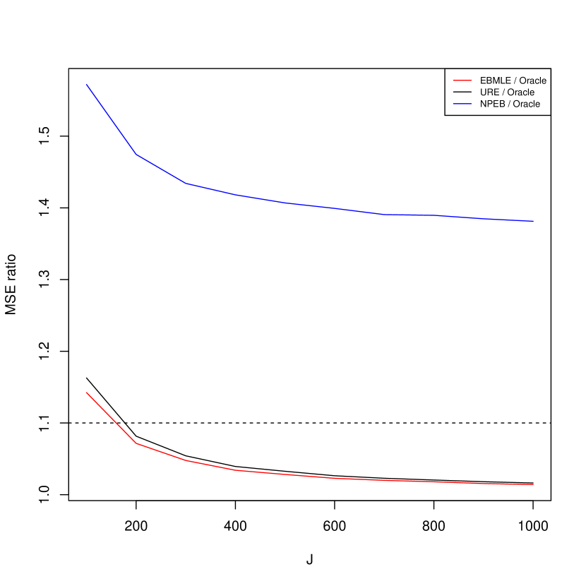
(a) Normal-Normal

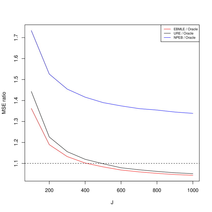
(b) Uniform-Normal

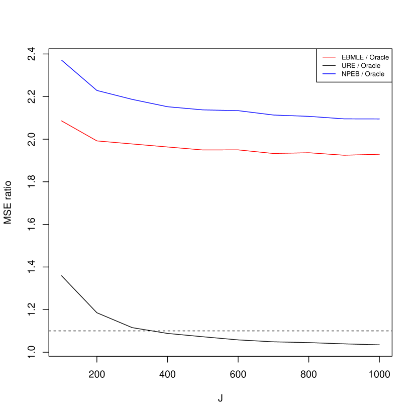
(c) Normal-Normal with group structure

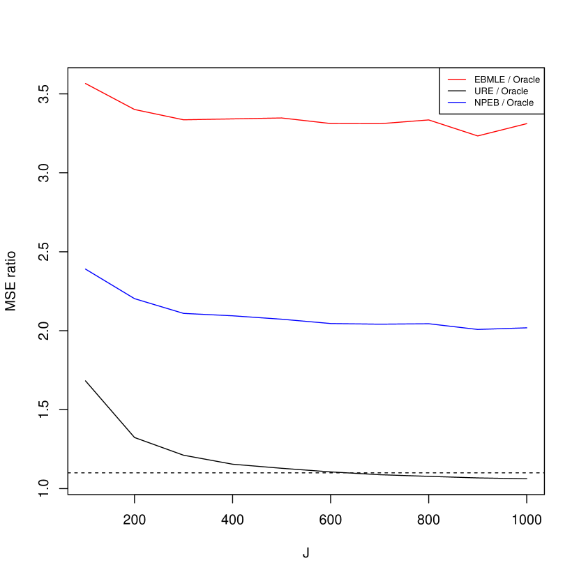
(d) Conditional Heteroskedasticity

Figure 5: Simulation results for the four main scenarios, including results from implementing the NPEB. Each plot has a black line, red line and a blue line, which correspond to the MSE of the URE, EBMLE and NPEB respectively, as a fraction of the oracle MSE. The x-axis is the sample size from $J=100$ to $1000$. The dotted line is a horizontal line at $1.1$ plotted to see when the MSE of the URE gets within 10% of the oracle.

Appendix E Weighted MSE

Here, I consider the case where the loss function is weighted in the sense

$$R(\theta,\widehat{\theta})=\textstyle\frac{1}{J}\operatorname{\mathbf{E}}_{\theta}(\widehat{\theta}-\theta)^{\prime}W(\widehat{\theta}-\theta),$$

where $W$ is a positive semidefinite $T\times T$ matrix. While I assume that the weight is the same for each $j$, all results in this section go though if one allows a different weight $W_{j}$ for each $j$ as long as $\sup_{j}\sigma_{1}(W_{j})<\infty.$

The corresponding risk estimate is given as

$$\mathbf{URE}^{W}_{j}(\mu,\Lambda)$$

$$= \operatorname{\mathrm{tr}}(W\Sigma_{j})-2\operatorname{\mathrm{tr}}((\Lambda+\Sigma_{j})^{-1}\Sigma_{j}W\Sigma_{j})$$

$$+(y_{j}-\mu)^{\prime}[(\Lambda+\Sigma_{j})^{-1}\Sigma_{j}W\Sigma_{j}(\Lambda+\Sigma_{j})^{-1}](y_{j}-\mu).$$

It is straightforward to see that analogous versions of Theorems 4.1, 4.2, and 4.3 go through for any positive semidefinite weight matrix $W$, which implies that minimizing the risk estimate obtains the oracle under weighted losses as well. To see this, note that the difference between the risk estimate and the loss is given as

$$\begin{aligned} &\mathbf{URE}^{W}_{j}(\mu,\Lambda)-(\widehat{\theta}_{j}(\mu,\Lambda)-\theta_{j})^{\prime}W(\widehat{\theta}_{j}(\mu,\Lambda)-\theta_{j})\\ =&\operatorname{\mathrm{tr}}(W\Sigma_{j})-2\operatorname{\mathrm{tr}}((\Lambda+\Sigma_{j})^{-1}\Sigma_{j}W\Sigma_{j})\\ &+(y_{j}-\mu)^{\prime}[(\Lambda+\Sigma_{j})^{-1}\Sigma_{j}W\Sigma_{j}(\Lambda+\Sigma_{j})^{-1}](y_{j}-\mu)\\ &-(y_{j}-\theta_{j}-\Sigma_{j}(\Lambda+\Sigma_{j})^{-1}(y_{j}-\mu))^{\prime}W(y_{j}-\theta_{j}-\Sigma_{j}(\Lambda+\Sigma_{j})^{-1}(y_{j}-\mu))\\ =&\operatorname{\mathrm{tr}}(W\Sigma_{j})-2\operatorname{\mathrm{tr}}((\Lambda+\Sigma_{j})^{-1}\Sigma_{j}W\Sigma_{j})-(y_{j}-\theta_{j})^{\prime}W(y_{j}-\theta_{j})\\ &+2(y_{j}-\mu)^{\prime}(\Lambda+\Sigma_{j})^{-1}\Sigma_{j}W(y_{j}-\theta_{j})\\ =&y_{j}^{\prime}Wy_{j}-\theta_{j}^{\prime}W\theta_{j}-\operatorname{\mathrm{tr}}(W\Sigma_{j})-2\operatorname{\mathrm{tr}}(W\Lambda(\Lambda+\Sigma_{j})^{-1}(y_{j}y_{j}^{\prime}-y_{j}\theta_{j}^{\prime}-\Sigma_{j}))\\ &-2\mu^{\prime}(\Lambda+\Sigma_{j})^{-1}\Sigma_{j}W(y_{j}-\theta_{j}).\end{aligned}$$ (38)

Since $W$ does not vary with $j$, the exact same proofs given for the theorems under $W=I_{T}$ all go through without any additional assumptions. Since the proof is essentially just a repetition of the provided proofs with additional $\sigma_{1}(W)$ terms appearing in numerous places, I omit the proof for the weighted case.

To see why considering weighted loss functions can be interesting, let $Q$ denote any $R\times T$ matrix, and suppose that the interest is in estimating the linear combinations $\{Q\theta_{j}\}_{j=1}^{J}$ rather than the original vector of the true means. Under the second level model of $\theta_{j}\overset{\mathrm{i.i.d.}}{\sim}N(\mu,\Lambda)$, the posterior mean of the parameter of interest is given as $Q\widehat{\theta}_{j}(\mu,\Lambda)$ and the resulting loss is

$$\frac{1}{J}\sum_{j=1}^{J}(Q\widehat{\theta}_{j}(\mu,\Lambda)-Q\theta_{j})^{\prime}(Q\widehat{\theta}_{j}(\mu,\Lambda)-Q\theta_{j})$$

$$= \frac{1}{J}\sum_{j=1}^{J}(\widehat{\theta}_{j}(\mu,\Lambda)-\theta_{j})^{\prime}Q^{\prime}Q(\widehat{\theta}_{j}(\mu,\Lambda)-\theta_{j}),$$

which is the original loss function with weight matrix $W=Q^{\prime}Q$. Hence, the weighted loss function arises naturally whenever a linear function of the parameter is of interest.

Weighted loss in the unbalanced case. Suppose the empirical researcher is interested in a linear combination of the true mean vector under the unbalanced case. In such a scenario, the weights should be adjusted so that it reflects the missing cells. To see this, consider the case where $Q=\frac{1}{T}\mathbf{1}_{T}^{\prime}$ so that the interest is in the time average of the mean for each unit $j$. Consider the extreme case where there is only one observation available, at period $1$, for $j$. Then, if one does not wish to distinguish between different teachers, it seems reasonable that the parameter of interest in this case should be $\theta_{j1}$ rather than $\frac{1}{T}\theta_{j1}$. However, if the researcher mechanically takes $QO_{j}^{\prime}$, then she will end up with this latter term. When $Q$ is a row vector with only nonnegative entries, a natural way to resolve this is to rescale $QO_{j}$ so that the sum of its entries is equal to the sum of the entries of $Q$ by defining $Q^{o}_{j}=\frac{Q\mathbf{1}_{T}}{\mathbf{1}_{o_{j}}^{\prime}QO_{j}^{\prime}}QO_{j}^{\prime}$. Note that $\frac{Q\mathbf{1}_{T}}{\mathbf{1}_{o_{j}}^{\prime}QO_{j}^{\prime}}=T/o_{j}$ when $Q=\frac{1}{T}\mathbf{1}_{T}^{\prime}$, which gives the desired weighting.

In the general case where $Q$ is a $R\times T$ matrix with positive entries, the same can be achieved by scaling $QO_{j}^{\prime}$ so that the sum of all the entries are equal the sum of entries of $Q$. Accordingly, define the scaled version as $Q_{j}^{o}=\frac{\mathbf{1}^{\prime}_{R}Q\mathbf{1}_{T}}{\mathbf{1}^{\prime}_{R}QO_{j}^{\prime}\mathbf{1}_{o_{j}}}QO_{j}^{\prime}$ and the corresponding weight matrix $W^{o}_{j}=Q_{j}^{o}{}^{\prime}Q_{j}^{o}$. In this case, the risk estimate to be minimized is given as $\mathbf{URE}^{o,W}(\mu,\Lambda)=\frac{1}{J}\sum_{j=1}^{J}\mathbf{URE}_{j}^{o,W}(\mu,\Lambda)$, where

$$\mathbf{URE}_{j}^{o,W}(\mu,\Lambda):= \operatorname{\mathrm{tr}}(W^{o}_{j}\Sigma^{o}_{j})-2\operatorname{\mathrm{tr}}((\Lambda_{j}^{o}+\Sigma^{o}_{j})^{-1}\Sigma^{o}_{j}W^{o}_{j}\Sigma_{j}^{o})$$

$$+(y^{o}_{j}-\mu_{j}^{o})^{\prime}[(\Lambda_{j}^{o}+\Sigma^{o}_{j})^{-1}\Sigma^{o}_{j}W^{o}_{j}\Sigma_{j}^{o}(\Lambda_{j}^{o}+\Sigma^{o}_{j})^{-1}](y^{o}_{j}-\mu^{o}).$$

Again, this risk estimate can be shown to converge uniformly to the corresponding loss

$$\frac{1}{J}\sum_{j=1}^{J}(\widehat{\theta}_{j}^{o}(\mu,\Lambda)-\theta_{j}^{o})^{\prime}W_{j}^{o}(\widehat{\theta}_{j}^{o}(\mu,\Lambda)-\theta_{j}^{o}).$$

Appendix F Computation

The URE estimators involve solving a minimization problem over $\Lambda\in\mathcal{L}$, along with possibly an additional hyperparameter that governs the centering term. For concreteness, I consider the estimator $\widehat{\theta}^{\mathrm{URE},\mathrm{g}}$ and take $\mathcal{L}=\mathcal{S}_{T}^{+}$.

The minimization problem that must be solved is

$$\inf_{\Lambda\in\mathcal{S}_{T}^{+},\mu\in\mathcal{M}_{J}}\mathrm{URE}(\mu,\Lambda).$$

For a fixed $\Lambda$, minimization with respect to $\mu$ is a quadratic programming program with bound constraints, which is a well understood problem with a number of efficient algorithms readily available. Hence, to utilize this quadratic structure with respect to $\mu$, I profile out $\mu$ by solving this quadratic programming problem. Writing $\mu^{\ast}(\Lambda):=\inf_{\mu}\mathrm{URE}(\mu,\Lambda)$, the problem is to now solve

$$\inf_{\Lambda\in\mathcal{S}_{T}^{+}}\,\,\mathrm{URE}(\mu^{\ast}(\Lambda),\Lambda).$$

This is a nonconvex optimization problem with nonlinear constraints, where the nonlinearity of the constraints is due to the restriction that $\Lambda$ is positive semidefinite. I transform this to a unconstrained problem by using the Cholesky decomposition by defining $f(L):=\mathrm{URE}(\mu^{\ast}(LL^{\prime}),LL^{\prime})$ and minimizing $f$ over all lower triangle matrices $L$ (i.e., over $\mathbf{R}^{T(T+1)/2}$). Using Quasi-Newton methods such as the BFGS algorithm works well on this transformed problem, finding the minimum within reasonable time without being sensitive to the initial point.

Each evaluation of the objective function involves calculating the inverse of $(\Lambda+\Sigma_{j})^{-1}$ for all $j$. That is, each evaluation involves inverting a $T\times T$ matrix $J$ times, which is unavoidable. Since even the state-of-the-art algorithms have computational complexity around $O(T^{2.4})$ for inverting a $T\times T$ matrix, the computation burden increases quickly with $T$ (and with $J$, of course, but to a much lesser extent). Nonetheless, the computation is not an issue for moderately large $T$. In the empirical example with around $J=1,200$ and $T=6$, calculating $\widehat{\theta}^{\mathrm{URE},\mathrm{g}}$ takes around 100 seconds on a single core using the companion R package.

Appendix G Details for the empirical exercise

G.1 Estimation of $\beta$ and $\sigma^{2}$

The coefficient vector on the observables, $\beta$, is estimated by OLS on the following demeaned version of the regression formula,

$$\widetilde{y}_{ijt}=\widetilde{X}_{ijt}^{\prime}\beta+\widetilde{\varepsilon}_{ijt},$$

so that $\widehat{\beta}=(\sum_{j=1}^{J}\sum_{t=1}^{T}\sum_{i=1}^{n_{jt}}\widetilde{X}_{ijt}\widetilde{X}_{ijt}^{\prime})^{-1}(\sum_{j=1}^{J}\sum_{t=1}^{T}\sum_{i=1}^{n_{jt}}\widetilde{X}_{ijt}\widetilde{y}_{ijt})$. The coefficient estimates are reported in Table 1. The variance of the idiosyncratic term $\sigma$ is estimated by dividing the sum of squared residuals by the appropriate degrees of freedom,

$$\widehat{\sigma}:=\frac{1}{\sum_{j=1}^{J}\sum_{t=1}^{T}(n_{jt}-1)-10}\sum_{j=1}^{J}\sum_{t=1}^{T}\sum_{i=1}^{n_{jt}}(\widetilde{y}_{ijt}-\widetilde{X}_{ijt}^{\prime}\widehat{\beta})^{2}$$

Table 1: Parameter estimates for the baseline value-added model (10).

	Dependent variable:
	ELA score	Math score
Score from previous year	$0.629^{***}$	$0.707^{***}$
	$(0.002)$	$(0.002)$
Male	$-0.069^{***}$	$0.022^{***}$
	$(0.003)$	$(0.002)$
Black	$-0.090^{***}$	$-0.112^{***}$
	$(0.006)$	$(0.005)$
Hispanic	$-0.060^{***}$	$-0.065^{***}$
	$(0.005)$	$(0.004)$
Asian	$0.071^{***}$	$0.122^{***}$
	$(0.005)$	$(0.004)$
Multi-Racial	$0.016$	$0.009$
	$(0.014)$	$(0.012)$
Native American	$-0.023$	$-0.018$
	$(0.015)$	$(0.013)$
ELL	$-0.180^{***}$	$-0.111^{***}$
	$(0.006)$	$(0.004)$
SWD	$-0.263^{***}$	$-0.207^{***}$
	$(0.005)$	$(0.004)$
FL	$-0.046^{***}$	$-0.042^{***}$
	$(0.003)$	$(0.003)$
Observations	174,239	195,792
Note: ∗p$<$0.1; ∗∗p$<$0.05; ∗∗∗p$<$0.01

G.2 Definition of the estimators for fixed effects

The least squares estimator for the time-varying fixed effect $\alpha_{jt}$ is given as

$$\widehat{\alpha}_{jt}=\frac{1}{n_{jt}}\sum_{i=1}^{n_{jt}}\left(\widetilde{y}_{ijt}-\widetilde{X}_{ijt}^{\prime}\widehat{\beta}\right),$$

and for the time-invariant case, $\widehat{\alpha}_{j0}=\frac{1}{n_{j}}\sum_{t=1}^{T}n_{jt}\widehat{\alpha}_{jt}$ with $n_{j}=\sum_{t=1}^{T}n_{jt}$.

The EBMLE for the time invariant case (i.e. the “conventional estimator”) is defined as $\widehat{\alpha}_{j0}^{\mathrm{EBMLE}}=\frac{\widehat{\sigma}/n_{j}}{\widehat{\sigma}/n_{j}+\widehat{\lambda}^{\mathrm{EBMLE}}}\widehat{\mu}^{\mathrm{EBMLE}}+\frac{\widehat{\lambda}^{\mathrm{EBMLE}}}{\widehat{\sigma}/n_{j}+\widehat{\lambda}^{\mathrm{EBMLE}}}\widehat{\alpha}_{j0}$, where $(\widehat{\mu}^{\mathrm{EBMLE}},\widehat{\lambda}^{\mathrm{EBMLE}})$ is obtained by maximizing the likelihood of $\widehat{\alpha}_{j0}$ given by $\widehat{\alpha}_{j0}\overset{\mathrm{indep}}{\sim}N\left(\mu,\frac{\widehat{\sigma}}{n_{j}}+\lambda\right)$.

To describe the estimators for the time variant case, write $\widehat{\Sigma}_{j}=\mathrm{diag}(\widehat{\sigma}/n_{j1},\dots,\widehat{\sigma}/n_{jT})$. The EBMLE and URE estimators for $\alpha_{j}$ in this case is given by

$$\Sigma_{j}(\widehat{\Lambda}+\Sigma_{j})^{-1}\widehat{\mu}+\widehat{\Lambda}(\widehat{\Lambda}+\Sigma_{j})^{-1}\widehat{\alpha}_{j}$$

where $(\widehat{\mu},\widehat{\Lambda})$ is chosen by maximizing the likelihood implied by $\widehat{\alpha}_{j}\overset{\mathrm{indep}}{\sim}N(\mu,\Lambda+\Sigma_{j})$ for EBMLE, and by minimizing $\mathrm{URE}(\mu,\Lambda)$ for the URE estimator with $\widehat{\alpha}_{j}$ playing the role of $y_{j}$ in the definition of $\mathrm{URE}(\mu,\Lambda)$.

Appendix H Semiparametric shrinkage

Here, I illustrate how the semiparametric shrinkage idea by Xie et al. (2012) can be extended to this setting. I consider the simple shrinkage estimator that shrinks to the origin. For the univariate model where $T=1$, the shrinkage estimator that shrinks to the origin can be written as

$$\widehat{\theta}(0,\Lambda)=\frac{\Lambda}{\Lambda+\Sigma_{j}}y_{j}.$$

Hence, the estimator is obtained by multiplying a shrinkage factor to the observation. This shinkage factor lies in $[0,1]$ and shrinks the decreases in $\Sigma_{j}$. Motivated by such observation, Xie et al. (2012) consider a class of semiparametric shrinkage estimators,

$$\widehat{\theta}^{b}(0,\Lambda)=b(\Sigma_{j})y_{j},$$

where $b(\cdot)$ is a weakly decreasing function taking values in $[0,1]$.

To extend this idea to the multivariate setting, recall that the shrinkage matrix is given as

$$\Lambda(\Lambda+\Sigma_{j})^{-1}=\Lambda^{\frac{1}{2}}(I+\Lambda^{-\frac{1}{2}}\Sigma_{j}\Lambda^{-\frac{1}{2}})^{-1}\Lambda^{-\frac{1}{2}}.$$

Replacing the middle term $(I+\Lambda^{-\frac{1}{2}}\Sigma_{j}\Lambda^{-\frac{1}{2}})^{-1}$ by $B(\Lambda^{-\frac{1}{2}}\Sigma_{j}\Lambda^{-\frac{1}{2}})$ where $B:\mathcal{S}_{T}^{+}\to\mathcal{S}_{T}^{+}$ is decreasing (with respect to the partial ordering $\leq$) and $\sigma_{1}(B(\cdot))\leq 1$ is a direct extension of the univariate case.

However, here I assume an additional Lipschitz condition, with known finite Lipschitz constant, on the function $B(\cdot)$ because 1) the partial ordering may end up imposing no restriction at all resulting in severe overfitting and 2) to invoke a uniform convergence result, it is convenient to have a totally bounded parameter space, which can be obtained by giving a bound on the Lipschitz constant of $B(\cdot)$. Under this bound and Assumption 4.1, the URE method (and the corresponding optimality) can be extended to this wider class of estimators in a straightforward manner. Note that the part of the shrinkage matrix we are relaxing, $(I+\Lambda^{-\frac{1}{2}}\Sigma_{j}\Lambda^{-\frac{1}{2}})^{-1}$, is Lipschitz as well, so the parametric estimator considered in the main text is indeed nested in this semiparametric class. However, computation is extremely difficult; the optimization problem that must be solved is with respect to a $T(T+1)/2$ matrix and a function of $T(T+1)/2$ variables.

References

- Abadie and Kasy (2019) Abadie, A. and M. Kasy (2019): “Choosing Among Regularized Estimators in Empirical Economics: The Risk of Machine Learning,” The Review of Economics and Statistics, 101, 743–762.
- Abaluck et al. (2020) Abaluck, J., M. M. C. Bravo, P. Hull, and A. Starc (2020): “Mortality Effects and Choice Across Private Health Insurance Plans,” Tech. Rep. w27578, National Bureau of Economic Research, Cambridge, MA.
- Abowd et al. (1999) Abowd, J. M., F. Kramarz, and D. N. Margolis (1999): “High Wage Workers and High Wage Firms,” Econometrica, 67, 251–333.
- Andrews (1992) Andrews, D. W. (1992): “Generic Uniform Convergence,” Econometric Theory, 8, 241–257.
- Angrist et al. (2017) Angrist, J. D., P. D. Hull, P. A. Pathak, and C. R. Walters (2017): “Leveraging Lotteries for School Value-Added: Testing and Estimation,” The Quarterly Journal of Economics, 132, 871–919.
- Armstrong et al. (2020) Armstrong, T. B., M. Kolesár, and M. Plagborg-Møller (2020): “Robust Empirical Bayes Confidence Intervals,” arXiv:2004.03448 [econ, stat].
- Banerjee et al. (2020) Banerjee, T., L. J. Fu, G. M. James, and W. Sun (2020): “Nonparametric empirical bayes estimation on heterogeneous data,” arXiv preprint arXiv:2002.12586.
- Bitler et al. (2019) Bitler, M., S. Corcoran, T. Domina, and E. Penner (2019): “Teacher Effects on Student Achievement and Height: A Cautionary Tale,” Tech. Rep. w26480, National Bureau of Economic Research, Cambridge, MA.
- Bonhomme and Weidner (2019) Bonhomme, S. and M. Weidner (2019): “Posterior Average Effects,” arXiv:1906.06360 [econ, stat].
- Brown and Greenshtein (2009) Brown, L. D. and E. Greenshtein (2009): “Nonparametric Empirical Bayes and Compound Decision Approaches to Estimation of a High-Dimensional Vector of Normal Means,” The Annals of Statistics, 37, 1685–1704.
- Brown et al. (2018) Brown, L. D., G. Mukherjee, and A. Weinstein (2018): “Empirical Bayes Estimates for a Two-Way Cross-Classified Model,” The Annals of Statistics, 46, 1693–1720.
- Chen (2022) Chen, J. (2022): “Gaussian Heteroskedastic Empirical Bayes without Independence,” arXiv preprint arXiv:2212.14444.
- Chetty et al. (2014a) Chetty, R., J. N. Friedman, and J. E. Rockoff (2014a): “Measuring the Impacts of Teachers I: Evaluating Bias in Teacher Value-Added Estimates,” American Economic Review, 104, 2593–2632.
- Chetty et al. (2014b) ——— (2014b): “Measuring the Impacts of Teachers II: Teacher Value-Added and Student Outcomes in Adulthood,” American Economic Review, 104, 2633–2679.
- Chetty and Hendren (2018) Chetty, R. and N. Hendren (2018): “The Impacts of Neighborhoods on Intergenerational Mobility II: County-Level Estimates,” The Quarterly Journal of Economics, 133, 1163–1228.
- Fessler and Kasy (2019) Fessler, P. and M. Kasy (2019): “How to Use Economic Theory to Improve Estimators: Shrinking Toward Theoretical Restrictions,” The Review of Economics and Statistics, 101, 681–698.
- Gilraine et al. (2020) Gilraine, M., J. Gu, and R. McMillan (2020): “A New Method for Estimating Teacher Value-Added,” Tech. Rep. w27094, National Bureau of Economic Research, Cambridge, MA.
- Guarino et al. (2015) Guarino, C. M., M. Maxfield, M. D. Reckase, P. N. Thompson, and J. M. Wooldridge (2015): “An Evaluation of Empirical Bayes’s Estimation of Value-Added Teacher Performance Measures,” Journal of Educational and Behavioral Statistics, 40, 190–222.
- Hansen (2016) Hansen, B. E. (2016): “Efficient Shrinkage in Parametric Models,” Journal of Econometrics, 190, 115–132.
- Hanushek (2011) Hanushek, E. A. (2011): “The Economic Value of Higher Teacher Quality,” Economics of Education Review, 30, 466–479.
- Horn and Johnson (1990) Horn, R. A. and C. R. Johnson (1990): Matrix Analysis, Cambridge University Press.
- Hull (2020) Hull, P. (2020): “Estimating Hospital Quality with Quasi-Experimental Data,” working paper.
- Ignatiadis and Wager (2020) Ignatiadis, N. and S. Wager (2020): “Covariate-Powered Empirical Bayes Estimation,” arXiv:1906.01611 [stat].
- James and Stein (1961) James, W. and C. Stein (1961): “Estimation with Quadratic Loss,” in Proceedings of the Fourth Berkeley Symposium on Mathematical Statistics and Probability, Volume 1: Contributions to the Theory of Statistics, The Regents of the University of California.
- Jiang and Zhang (2009) Jiang, W. and C.-H. Zhang (2009): “General Maximum Likelihood Empirical Bayes Estimation of Normal Means,” The Annals of Statistics, 37, 1647–1684.
- Kane et al. (2008) Kane, T. J., J. E. Rockoff, and D. O. Staiger (2008): “What Does Certification Tell Us about Teacher Effectiveness? Evidence from New York City,” Economics of Education Review, 27, 615–631.
- Kling (2006) Kling, J. R. (2006): “Incarceration Length, Employment, and Earnings,” American Economic Review, 96, 24.
- Koedel et al. (2015) Koedel, C., K. Mihaly, and J. E. Rockoff (2015): “Value-Added Modeling: A Review,” Economics of Education Review, 47, 180–195.
- Koenker and Mizera (2014) Koenker, R. and I. Mizera (2014): “Convex Optimization, Shape Constraints, Compound Decisions, and Empirical Bayes Rules,” Journal of the American Statistical Association, 109, 674–685.
- Kong et al. (2017) Kong, X., Z. Liu, P. Zhao, and W. Zhou (2017): “SURE Estimates under Dependence and Heteroscedasticity,” Journal of Multivariate Analysis, 161, 1–11.
- Kou and Yang (2017) Kou, S. C. and J. J. Yang (2017): “Optimal Shrinkage Estimation in Heteroscedastic Hierarchical Linear Models,” in Big and Complex Data Analysis, ed. by S. E. Ahmed, Cham: Springer International Publishing, 249–284.
- Li (1985) Li, K.-C. (1985): “From Stein’s Unbiased Risk Estimates to the Method of Generalized Cross Validation,” The Annals of Statistics, 13, 1352–1377.
- Liu et al. (2020) Liu, L., H. R. Moon, and F. Schorfheide (2020): “Forecasting With Dynamic Panel Data Models,” Econometrica, 88, 171–201.
- Okolewski and Rychlik (2001) Okolewski, A. and T. Rychlik (2001): “Sharp Distribution-Free Bounds on the Bias in Estimating Quantiles via Order Statistics,” Statistics & Probability Letters, 52, 207–213.
- Robbins (1951) Robbins, H. (1951): “Asymptotically Subminimax Solutions of Compound Statistical Decision Problems,” in Proceedings of the Second Berkeley Symposium on Mathematical Statistics and Probability, The Regents of the University of California.
- Robbins (1964) ——— (1964): “The Empirical Bayes Approach to Statistical Decision Problems,” Annals of Mathematical Statistics, 35, 1–20.
- Rockoff (2004) Rockoff, J. E. (2004): “The Impact of Individual Teachers on Student Achievement: Evidence from Panel Data,” American Economic Review, 94, 247–252.
- Rothstein (2010) Rothstein, J. (2010): “Teacher Quality in Educational Production: Tracking, Decay, and Student Achievement,” The Quarterly Journal of Economics, 125, 175–214.
- Stein (1956) Stein, C. (1956): “Inadmissibility of the Usual Estimator for the Mean of a Multivariate Normal Distribution,” in Proceedings of the Third Berkeley Symposium on Mathematical Statistics and Probability, Volume 1: Contributions to the Theory of Statistics, The Regents of the University of California.
- Wooldridge (2010) Wooldridge, J. M. (2010): Econometric Analysis of Cross Section and Panel Data, MIT Press.
- Xie et al. (2016) Xie, X., S. C. Kou, and L. Brown (2016): “Optimal Shrinkage Estimation of Mean Parameters in Family of Distributions with Quadratic Variance,” The Annals of Statistics, 44, 564–597.
- Xie et al. (2012) Xie, X., S. C. Kou, and L. D. Brown (2012): “SURE Estimates for a Heteroscedastic Hierarchical Model,” Journal of the American Statistical Association, 107, 1465–1479.