Lightweight Materialization for Fast Dashboards Over Joins

Abstract.

Dashboards are vital in modern business intelligence tools, providing non-technical users with an interface to access comprehensive business data. With the rise of cloud technology, there is an increased number of data sources to provide enriched contexts for various analytical tasks, leading to a demand for interactive dashboards over a large number of joins. Nevertheless, joins are among the most expensive operations in DBMSes, making the support of interactive dashboards over joins challenging.

In this paper, we present Treant, a dashboard accelerator for queries over large joins. Treant uses factorized query execution to handle aggregation queries over large joins, which alone is still insufficient for interactive speeds. To address this, we exploit the incremental nature of user interactions using Calibrated Junction Hypertree (CJT), a novel data structure that applies lightweight materialization of the intermediates during factorized execution. CJT ensures that the work needed to compute a query is proportional to how different it is from the previous query, rather than the overall complexity. Treant manages CJTs to share work between queries and performs materialization offline or during user "think-times." Implemented as a middleware that rewrites SQL, Treant is portable to any SQL-based DBMS. Our experiments on single node and cloud DBMSes show that Treant improves dashboard interactions by two orders of magnitude, and provides $10{\times}$ improvement for ML augmentation compared to SOTA factorized ML system.

1. Introduction

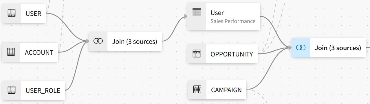
(a) Build join graph offline by data engineering. Three tables related to User are first joined. Then, the enriched User table is joined with Opportunity and Campaign.

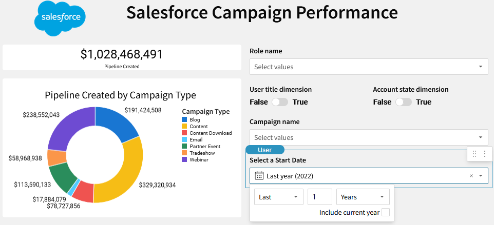
(b) Dashboard interface for online exploration.

Figure 1. Screenshots for Sigma Computing dashboards.

Dashboards are at the heart of modern BI tools (e.g., PowerBI (powerbi, ), Looker (looker, ), Sigma Computing (gale2020sigma, )) and provide a comprehensive view of a business within a single interface. Modern organizations store data across dozens or hundreds of tables in data warehouses, so dashboard creation consists of two stages. Offline, data engineers pre-define join relationships between relevant tables so that they can be queried like a denormalized “wide table”, and create dashboard visualizations. Online, domain users interact with the dashboards and make business decisions. For example, let’s consider a hypothetical scenario based on Sigma Computing:

Example 1 (Sigma Computing Dashboard).

Anna, a sales manager, is responsible for driving revenue growth. To gain a better understanding of the current state of the business, she asks Shannon, a data engineer, to build a dashboard to display sales pipelines for potential revenue opportunities. Shannon collects relevant tables from Salesforce (e.g., Opportunities, Campaigns, Users) for deals from various sales representatives, and creates the join graph $R_{\Join}$ shown in Figure 1(a).

Shannon designs the dashboard in Figure 1(b), where each chart is generated from an initial dashboard query, and interactions change parts of those queries to update the charts. The total "Pipeline Created" is computed by $Q_{1}{=}\gamma_{SUM(amount)}R_{\Join}$ while the pie chart displaying "Pipeline Created by Campaign Type" is computed by $Q_{2}{=}\gamma_{SUM(amount),Campaign\_Type}R_{\Join}$. Shannon adds interactions (e.g., dropdown boxes and switches) to filter or change the grouping attributes. For example, selecting “Sales Associate” in the “Role Name” dropdown triggers an interaction query that filters $R_{\Join}$ by the role before aggregating the data for $Q_{1},Q_{2}$, while toggling the “User Title” switch adds the attribute to the group by. However, every interaction translates to queries over the join graph that take many seconds to complete, causing Anna to stop using the dashboard.

The pattern in the above example is common. Data engineers build a dashboard over a complex acyclic join graph. When a domain user loads the dashboard, it first executes the dashboard queries to load the initial view, and then executes many interaction queries in response to user manipulations. Each of the interaction queries is similar to the dashboard queries, but may add/change a filter, grouping attribute, or add/remove a relation. The key challenge is that users expect fast response times (liu2014effects, ), yet joins are notoriously expensive to execute (leis2018query, ; neumann2018adaptive, ; albutiu2012massively, ). Traditional techniques, like cubing (gray1997data, ) and indexing (moritz2019falcon, ), are designed for a single table, but poorly handle joins because the denormalized table size can be exponential to the number of relations: $O(n\times f^{r})$, where $f$ is the fanout along join graph edges with $r$ relations, each of size $n$.

Recent factorized query execution techniques (olteanu2015size, ; aberger2017emptyheaded, ) speed up queries over large joins by pushing down aggregation through the joins, in the spirit of projection pushdown. This reduces the space overhead (for acyclic joins) to a linear scale: $O(rn)$, making it promising for developing interactive dashboards. However, naive factorized query execution of interaction queries online still results in high latency. The process requires scanning, joining, and aggregating all the relations as part of the factorized query execution, which prevents achieving interactive speeds. Recent work (schleich2019layered, ) has proposed optimizing a pre-determined batch of factorized queries offline. However, interaction queries are only determined by the combination of user interactions online. Batching all possible interaction queries offline would lead to a combinatorially large overhead.

In this paper, we present Treant, a dashboard accelerator for interaction queries over large joins. Offline, the engineering team connects Treant to a DBMS, specifies the join graph (tables and join conditions), and defines Selection-Projection-Join-Aggregation (SPJA) queries (potentially from a BI dashboarding tool) as dashboard queries to create visualizations. Treant precomputes compact data structures and stores them as tables in the DBMS; this incurs a constant factor runtime cost relative to running the dashboard queries. Online, Treant supports a wide range of interaction queries that modify select/group clauses, update or remove tables, or join new tables to the dashboard queries, all at interactive speeds.

To support efficient aggregation queries over joins, we observe that interaction queries differ from the dashboard query by keeping the query structure but modifying a subset of the SPJA operators. To this end, we introduce the novel Calibrated Junction Hypertree (CJT) data structure to support work sharing and ensure that the work needed to compute an interaction query is proportional to how different it is from its corresponding dashboard query (or interaction query), rather than its overall complexity. Our design builds on the observation by Abo et al. (abo2016faq, ) that factorized query execution can be modeled as message passing in Probabilistic Graphical Models (PGM) (koller2009probabilistic, ), as described in the following example:

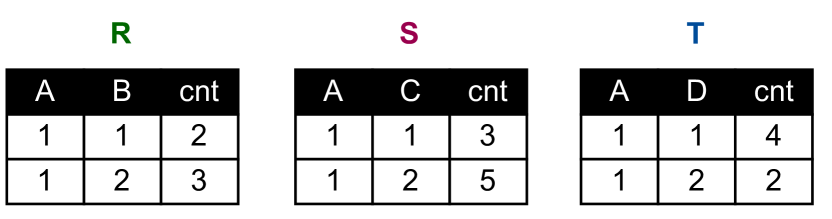
(a) Relations.

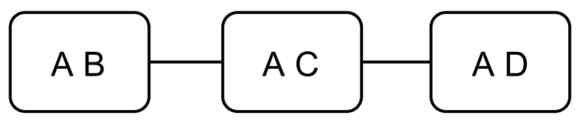
(b) Join graph.

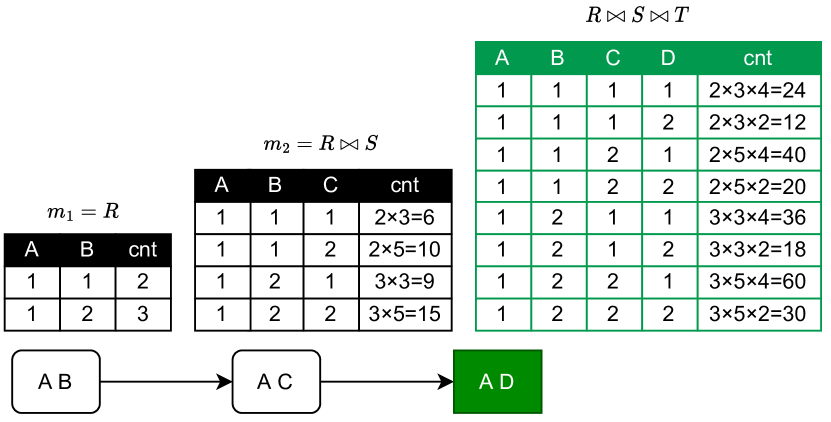
(c) Naive query execution. The full join result is in green.

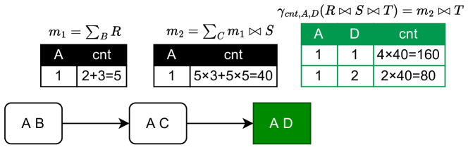
(d) Upward message passing. The final result is in green.

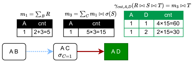
(e) $m_{1}$ (dotted blue) could be re-used for interaction query with additional selection $\sigma_{C{=}1}$ and only $m_{3}$ (red) need to be computed.

Figure 2. Example database with three relations, its join graph (also JT), naive query execution for the total count, and factorized query execution by upward message passing.

Example 2.

Figure 2(a,b) list example relations (duplicates are tracked with a cnt “annotation”) and the join graph, respectively. Consider a dashboard query that computes the total count over the full join result: $Q=\gamma_{cnt}(R\Join S\Join T)$. Figure 2(c) naively executes the query, which computes the full join in order $(R\Join S)\Join T$ before summing the counts, and requires exponential space.

In contrast, factorized query execution distributes the summation through joins, so that each node first sums out (marginalizes) attributes irrelevant downstream, and then emits a smaller message. Any sequence of messages from leaves to root in the join graph results in the correct result. Figure 2(d) chooses $T$ as the root, then passes messages along $R{\to}S{\to}T$. AB marginalizes out B and AC marginalizes out C. Therefore, we only sum 2 tuples to compute the final query result.

The benefit of viewing query execution as message passing is that work-sharing opportunities become self-evident. Consider the interaction query in Figure 2(e), which adds a predicate $C{=}1$ over $S[AC]$. Factorized query execution would re-pass messages along $R{\to}S{\to}T$, but misses the opportunity to reuse $m_{1}$. A partial solution is to cache the messages when executing dashboard query. However, message contents are sensitive to the message-passing order: if we executed the dashboard query along $T{\to}S{\to}R$, then the message between $R$ and $S$ would differ from $m_{1}$. Thus, interaction queries would be forced to use the same (possibly suboptimal) message passing order, or sacrifice message reuse. An alternative is to enumerate all orders and store their messages, but has compute and storage costs quadratic in the number of relations.

Our algorithmic contribution is to show that after executing the dashboard query, sending messages in reverse from root to leaves (e.g., $R{\leftarrow}S{\leftarrow}T$) is sufficient to support any execution order over the join graph. We, therefore, use CJT to proactively materialize dashboard query messages for all possible orders. Such a process is called "calibration" and is first brought up in PGM (shafer1990probability, ), which is used to similarly share computation between queries on posterior distributions. We are the first to apply it to SPJA queries.

CJTs allow work sharing between dashboard queries and interaction queries, and we further extend work sharing between interaction queries. The key idea is that, given dashboard query $q_{0}$, after a user performs an interaction (e.g., filter by Role as $q_{1}$), they may add another interaction (e.g., further add a filter by Campaign as $q_{2}$). In this case, the difference between the successive interaction queries ($q_{1}$ and $q_{2}$) is smaller than between $q_{2}$ and $q_{0}$. Since $q_{1}$ is not known offline, we calibrate it online during “think-time” between interactions (eichmann2020idebench, ). Such calibration doesn’t need to be fully completed, and the user’s next interaction preempts calibration. The next query can benefit from any messages that are newly materialized.

We implement Treant as a Python dashboard accelerator library. Treant acts as a middleware that transparently rewrites queries from dashboards to benefit from factorized execution and work sharing from CJTs. The generated queries are simple and easily ported to different DBMSes or data frame systems (reback2020pandas, ; modin, ). Furthermore, Treant accelerates advanced dashboard features like interactive Data Augmentation (chepurko2020arda, ) for analytics or machine learning.

To summarize, our contributions are as follows:

• We design the novel CJT data structure, which improves the efficiency of interaction queries over join by reusing messages and applying calibration. The cost of materializing the data structure is within a constant factor of the dashboard query execution, but accelerates interaction queries by multiple orders of magnitude.

• We build Treant, which manages CJT to transparently accelerate dashboards. It builds CJTs based on initial dashboard queries, and uses think time to further calibrate interaction queries. Its simple rewrite-based design is easily portable to any SQL-based DBMS.

• We evaluate the effectiveness of Treant on both local and cloud DBMSes using real-world dashboards and TPC benchmarks. Our results show that Treant accelerates most interaction queries by $>100\times$, and speeds up ML augmentation by $10{\times}$.

2. Background

This section provides a brief overview of annotated relations, early marginalization and variable elimination to accelerate join-aggregation queries, and the junction hypertree for join representation.

Data Model. Let uppercase symbol $A$ be an attribute, $dom(A)$ is its domain, and lowercase symbol $a\in dom(A)$ be a valid attribute value. For the purpose of analytical simplicity, we assume categorical attributes with a fixed domain size. Given relation R, its schema $S_{R}$ is a set of attributes, and its domain $dom(R)=\times_{A\in S}dom(A)$ is the Cartesian product of its attribute domains. An attribute is incident of R if $A\in S_{R}$. Given tuple t, let $t[A]$ be its value of attribute A.

Annotated Relations. Since relational algebra (first-order logic) does not support aggregation, it has been extended with the use of commutative structures to support aggregation. The main idea is that tuples are annotated with values from a semi-ring, and when relational operators (e.g., join, project, group-by) concatenate or combine tuples, they also multiply or add their annotations, such that the final annotations correspond to the aggregation results.

A commutative semi-ring $(D,+,\times,0,1)$ consists of a set $D$ and binary operators + and $\times$ that are commutative and closed over $D$, along with the zero $0$ and unit $1$ elements. We focus on semi-rings with elements in $D$ of constant size for efficiency. The semi-ring structure accommodates nearly all standard aggregates such as count, sum, min, max, etc (abo2016faq, ). More complex aggregates and even ML model can be constructed from semi-ring: variance can be derived from count, and sum ($var(A)=sum(A^{2})/count(A)-sum(A)^{2}/count(A)^{2}$), and linear regression can be trained based on the sum of pairwise products among features and target variable. There are two commonly used classes of aggregates not supported: percentile-based (e.g., median), and distinct-based (e.g., distinct count) aggregates. They require the tracking of a distribution or a unique value set, and cannot be represented by a set $D$ of constant-sized elements. These can be approximated for future work (cormode2011sketch, ). For simplicity, the text will be based on COUNT queries and the natural numbers semi-ring $(\mathbb{N},+,\times,0,1)$, which operates as in grade school math. Each relation $R$ annotates each of its tuples $t\in dom(R)$ with a natural number, and $R(t)$ refers to this annotation for tuple $t$ (green2007provenance, ; joglekar2015aggregations, ; nikolic2018incremental, ). We will use the terms relation and annotated relation interchangeably.

Semi-ring Aggregation Query. Aggregation queries are defined over annotated relations, and the relational operators are extended to add or multiple tuple annotations together, so that the output tuples’ annotations are the desired aggregated values.

Consider an example query $\gamma_{\textbf{A},\emph{COUNT}}(R_{1}\Join R_{2}...\Join R_{n})$ that joins $n$ relations, groups by a set of attributes A, and computes the COUNT. The operators that combine annotations are joins and groupbys and they compute the output tuple annotations as follows:

(1) $$(R\Join T)(t)= \hskip 5.0ptR(\pi_{S_{R}}(t))\times T(\pi_{S_{T}}(t))$$

(2) $$(\sum_{A}R)(t)= \sum\{R(t_{1})|\hskip 5.0ptt_{1}\in S_{R},t=\pi_{S_{R}\backslash\{A\}}(t_{1})\}$$

(1) states that given a join output tuple $t$, its annotation is the product of counts from the contribution pair of input tuples. (2) defines the count for output tuple $t$, and $\sum_{A}R$ denotes that we marginalize over $A$ and remove it from the output schema. This corresponds to summing the counts for all input tuples in the same group as $t$. In this paper, we assume natural joins with identical names for join keys for clarity. To summarize, join and groupby correspond to $\times$ and $+$, respectively. Let the schema of $R_{1}\Join R_{2}...\Join R_{n}$ be S. $q$ can be rewritten as $\sum_{A\in\textbf{S}-\textbf{A}}(R_{1}\Join R_{2}...\Join R_{n})$.

Early Marginalization. In simple algebra (as well as semi-rings), multiply distributes over addition, and can allow us to push marginalization through joins, in the spirit of projection push down (gupta1995aggregate, ).

Consider Figure 2, which computes $\gamma_{A;\emph{COUNT}}\left(R\Join S\Join T\right)$. We can rewrite it as marginalizing $B$, $C$, and $D$ from the full join result $\sum_{B}\sum_{C}\sum_{D}R[A,B]\Join S[A,C]\Join T[A,D].$ Although the naive cost is $O(n^{3})$ where $n$ is the relation size, we can push down marginalizations: $\sum_{D}({\color[rgb]{0.01,0.40,.8}\sum_{C}(}{\color[rgb]{1,0,0}(\sum_{B}R[A,B])}{\color[rgb]{0.01,0.40,.8}\Join S[A,C])}\Join T[A,D])$ where the largest intermediate result, and thus the join cost, is $O(n)$.

Join Ordering and Variable Elimination. Early marginalization is applied to a given join order. Thus we may also reorder the joins to cluster relations that involve a given attribute, so that it can be safely marginalized. Consider the query $\sum_{A}R[A,B]\Join S[B,D]\Join T[A,C]$. We can reorder the joins so that $A$ can be marginalized out earlier: $S[B,D]\Join\sum_{A}(R[A,B]\Join T[A,C]).$ The above procedure, where for each marginalized attribute $A$, we first cluster and join relations incident to $A$, and then marginalize $A$, is called variable elimination (cozman2000generalizing, ). Variable Elimination is widely used for PGM inference (koller2009probabilistic, ) and factorized execution (abo2016faq, ). Variable Elimination reduces the optimization to: (a) identifying the order in which attribute(s) are marginalized out (by clustering and joining the incident relations), and (b) determining the best arrangement of relations within the cluster. (b) is the traditional join ordering problem (steinbrunn1997heuristic, ). DBMSes that employ binary join use information such as relation cardinality to optimize the ordering. Prior works (abo2016faq, ; schleich2019layered, ) also apply worst-case-optimal-join (WCOJ (ngo2018worst, )) to simultaneously join these tables for asymptotic improvement. (a) is called the variable elimination order and its complexity is dominated by the intermediate join result size of the clustered relations (using WCOJ). It is well known that finding the optimal order (with the minimum intermediate size) is NP-hard (fischl2018general, ). However, common DBMS queries are over the acyclic join, whose optimal order could be found efficiently by GYO-elimination procedure (yu1979algorithm, ; abo2016faq, ). The central idea is to repeatedly: (1) eliminate attributes that are present in only one relation, and (2) join relations $R$ with $S$ if the schema of $R$ is a subset of $S$’s schema.

Example 3.

Consider $\sum_{ABCD}R[A,B]\Join S[B,C]\Join T[C,D]$, which is acyclic and we apply GYO-elimination: we first eliminate $A,D$ because they each only appear in one relation $R,T$ respectively (the order could also be $D,A$). This results in the intermediates $M_{1}[B],M_{2}[C]$, whose schemas are subsets of $S$. So we further join $M_{1}$, $M_{2}$, with $S$ and eliminate $B,C$. The final variable elimination order is $ADBC$:

$$\textstyle\sum_{DBC}S[B,C]\Join T[C,D]\Join{\color[rgb]{1,0,0}\textstyle\sum_{A}(R[A,B])}$$

$$= \textstyle\sum_{BC}S[B,C]\Join M_{1}[B]\Join{\color[rgb]{1,0,0}\textstyle\sum_{D}(T[C,D])}$$

$$= \textstyle\sum_{C}M_{2}[C]\Join{\color[rgb]{1,0,0}\textstyle\sum_{B}(S[B,C]\Join M_{1}[B])}={\color[rgb]{1,0,0}\textstyle\sum_{C}(M_{3}[C]\Join M_{2}[C])}$$

Each elimination step is highlighted in red.

Junction Hypertree. The Junction Hypertree (JT) is a representation of a join query that is amenable to complexity analysis (abo2016faq, ; joglekar2016ajar, ) and semi-ring aggregation query optimization (aberger2017emptyheaded, ). Given a join graph $R_{1}\Join\ldots\Join R_{n}$, JT is a pair $(E,V)$, where each vertex $v\in V$ is a subset of attributes in the join graph, and the undirected edges form a tree that spans the vertices. The join graph may be explicitly defined by a query, or induced by the foreign key relationships in a database schema. Following prior work (abo2016faq, ), a JT vertex is also called a bag. A JT must satisfy three properties:

• Vertex Coverage: The union of all bags in the tree must be equal to the set of attributes in the join graph.

• Edge Coverage: For every relation $R$ in the join graph, there exists at least one bag that is a superset of $R$’s attributes.

• Running intersection: For any attribute in the join graph, the bags containing the attribute must form a connected subtree.

The last property is important because JTs are related to variable elimination and are used for query execution. Given an elimination ordering, let each join cluster be a bag in the JT, and adjacent clusters be connected by an edge. In this context, executing the variable elimination order corresponds to traversing the tree (path); when execution moves beyond an attribute’s connected subtree, then it can be safely marginalized out. Note that since the JT is undirected, it can induce many variable elimination orders (execution plans) from a given JT, all with the same runtime complexity.

Finally, there are many valid JT for a given join graph, and the complexity (query execution cost) of a JT is dominated by the largest bag (the join size of the relations covered by the bag). Although finding the optimal JT for an arbitrary join graph is NP-hard (fischl2018general, ), we can trivially create the optimal JT for an acyclic join graph by creating one bag for each relation (e.g., the JT is simply the join graph) and the size of each bag is bounded by its corresponding relation size. We refer readers to FAQ (abo2016faq, ) for a complete description.

Message Passing for Query Execution. Message Passing was first introduced by Judea Pearl in 1982 (pearl1982reverend, ) (known as belief propagation) in order to efficiently perform inference (compute marginal probability) over probabilistic graphical models. In database terms, each probability table corresponds to a relation, the probabilistic graphical model corresponds to the full join graph in a database (as expressed by a JT), the joint probability over the model corresponds to the full join result, and marginal probabilities correspond to grouping over different sets of attributes. To further support semi-ring aggregation, Abo et al. (abo2016faq, ) established the equivalence between factorized query execution, and (upward) message passing. The full algorithm can be found in Appendix A; below, we illustrate how message passing over JT is used for query execution.

The procedure first determines a traversal order over the JT—since the JT is undirected, we can arbitrarily choose any bag as the root and create directed edges that point towards the root—and then traverses from leaves to root. We first compute the initial contents of each bag by joining the necessary relations based on the bag’s attributes. When we traverse an outgoing edge from a bag $l$ to its parent $p$, we marginalize out all attributes that are not in their intersection—the result is the Message between $l$ and $p$. The parent bag then joins the message with its contents. Each bag waits until it has received messages from all incoming edges before it emits along its outgoing edge. Once the root has received all incoming messages, its updated contents correspond to the query result.

Example 4 (Message Passing).

Consider the relations in Figure 2(a), and the JT in Figure 2(b) where each bag is a base relation. We wish to execute $\sum_{ABCD}R(A,B)\Join S(A,C)\Join T(A,D)$ by traversing along the path $R{\to}S{\to}T$ (Figure 2(d)). We first marginalize out $B$ from $AB$, so the message to $AC$ is a single row with count $5$. The bag $AC$ joins the row with its contents, and thus multiplies each of its counts by $5$. It then marginalizes out $C$, so its message to $AD$ is a single row with count $(3+5)\times 5$. Finally, bag $AD$ absorbs the message (Figure 2(d)) and marginalizes out $A$ and $D$ to compute the final result.

3. Calibrated Junction Hypertree

While message passing over JT exploits early marginalization to accelerate query execution, it has traditionally been limited to single-query execution. This section introduces Calibrated Junction Tree (CJT) to enable work-sharing for interactive dashboards on large joins. The idea is to materialize messages over the JT for dashboard query, and reuse a subset of its messages for interaction queries. This section will focus on the basis for the CJT data structure and how it is used to execute interaction queries. The next section will describe how Treant applies CJT to build an interactive dashboard.

Our novelty is (1) to use JTs as a concrete data structure to support message reuse, and (2) to borrow calibration (shafer1990probability, ) from PGM to materialize messages for any message passing order. Although CJT is widely used across engineering (zhu2015junction, ; ramirez2009fault, ), ML (braun2016lifted, ; deng2014large, ), and medicine (pineda2015novel, ; lauritzen2003graphical, ), it was used only for probabilistic inference (sum over probability); we are the first to extend it to general SPJA queries with semi-ring aggregations in DBMS for work sharing.

3.1. Motivating Example

We illustrate the work sharing between a dashboard query $Q_{1}=\sum_{ABCD}R(A,B)\Join S(A,C)\Join T(A,D)$, and an interaction query $Q_{2}=\sum_{ABCD}R(A,B)\Join{\color[rgb]{0.01,0.40,.8}\sigma_{C=1}}(S(A,C))\Join T(A,D)$ with additional predicate C=1, to motivate CJT.

Example 5.

Consider the JTs in Figure 3(a) which assign $AD$ as the root for $Q_{1},Q_{2}$ and traverse along the path $R\to S\to T$. Although the message $R\to S$ will be identical (blue edges), the additional filter over $S$ means that its outgoing message (and all subsequent messages) will differ from $Q_{1}$’s and cannot be reused (red edges). In contrast, Figure 3(b) uses $S$ as the root, so both messages can be reused and the $S$ bag simply applies the filter after joining its incoming messages.

This example shows that message reuse depends on how the root bag is chosen for dashboard query ($Q_{1}$), and for different interaction queries, we may wish to choose different roots. Since we don’t know the exact join, grouping, and filter criteria of future interaction queries, the naive solution is to (costly) materialize messages for all possible roots. We next present CJT, a novel data structure for query execution and message reuse, and address these limitations.

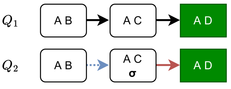
(a) Message passing to root AD.

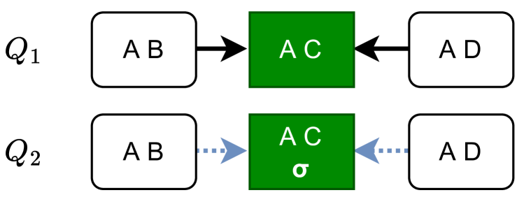
(b) Moving root increases reuse.

Figure 3. Work sharing between queries $Q_{1}$ (total count query) and $Q_{2}$ (additional selection to S). Dotted blue edges are reusable messages and solid red edges are non-reusable.

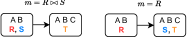
Figure 4. The same JT over relations R(A,B), S(A), T(B,C) can have different relation mappings ($\mathcal{X}$) and each mapping results in different messages ($m$). For each bag, its attributes are at the top and mapped relations are at the bottom.

3.2. Junction Hypertree as Data Structure

A naive approach to re-use messages is to execute an aggregation query over JT, and cache the messages; when a future query traverses an edge in the JT, it reuses the corresponding message. Unfortunately, this is 1) inaccurate, because messages generated along an edge are not symmetric and depend on the specific traversal order during message passing, 2) insufficient, because it cannot directly express filter-group-by queries, and 3) leaves performance on the table. To do so, we extend JT as follows:

Directed Edges. To support arbitrary traversal orders, we replace each undirected edge with two directed edges, and use $\mathcal{Y}(i\to j)$ to refer to the cached message for the directed edge $i\to j$.

Relation Mapping. $\mathcal{X}(R)$ maps each base relation $R$ to exactly one bag containing $R$’s schema. Although different mappings can lead to different messages (Figure 4), acyclic join graphs have a good default mapping where each bag is mapped by a single relation. Relations mapped to the same bag are joined during message passing.

Empty Bags. To avoid large paths during message passing, it’s beneficial to add custom empty bags to create “short cuts”. Empty bags are not mapped from any relations and are simply a mechanism to materialize custom views for work sharing. They join incoming messages, marginalize using standard rules, and materialize the outgoing messages. Empty bags are a novel addition in this work: previous works (abo2016faq, ; aberger2017emptyheaded, ; xirogiannopoulos2019memory, ) focus on non-redundant JT without empty bags. This is because they are in the context of single query optimization, where empty bags offer no advantage.

Example 6 (Empty Bag).

Consider the simplified TPC-DS JT in Figure 5(a). Store Sales is a large fact table (2.68M rows at SF=1), while the rest are much smaller. To accelerate a query that aggregates sales grouped by (Store,Time), we can create the empty bag Time Stores between Store_Sales, Time and Stores (Figure 5(b)). The message from Store_Sales to the empty bag is sufficient for the query and is $17.3\times$ smaller (154K rows) than the fact table.

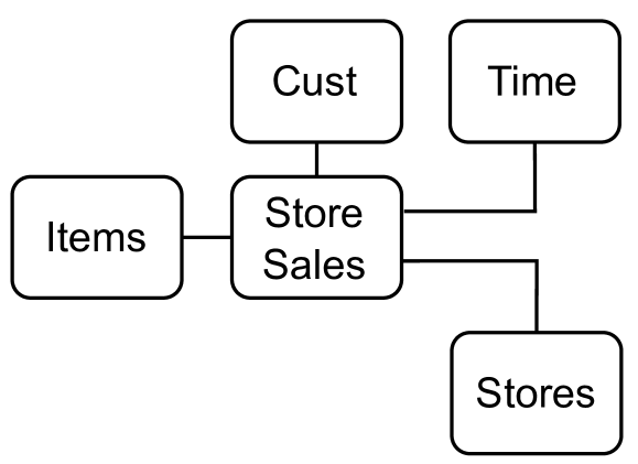
(a) TPC-DS join graph (also JT)

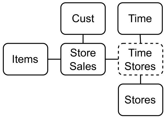
(b) Add empty bag (Time, Stores).

Figure 5. Simplified Join graph (JT) of TPC-DS. Adding an empty bag can accelerate queries group-by Time and Stores.

Note that leaf empty bag may result in an empty output message; we avoid this special case by mapping the identity relation $\mathcal{I}$ to it, such that $R\Join\mathcal{I}=R$ for any relation $R$. Essentially, the empty bag is “pass-through” and doesn’t change the join results nor the query result. When the bag is a leaf node, its message is simply $\mathcal{I}$. We do not materialize the identity relation, as it’s evident from the JT.

Example 7 (JT Data Structure).

Figure 6(b) illustrates the JT data structure for the example in Figure 2. Each relation maps to exactly one bag (orange dotted arrows), and each directed edge between bags (black arrows) stores its corresponding message (purple dashed arrows). Bag D (dotted rectangle) is an empty bag and materializes the view of "count group by D". $\mathcal{I}$ is the identity relation.

Annotation	Effect	Applicability	Section
$\gamma_{A}$	Prevent A from being marginalized out for all downstream bags.	Any bag containing A.	Section 3.3
$\sum_{A}$	Marginalize out $A$. “Cancels” $\gamma_{A}$ for downstream bags.	Any bag containing A.	Section 3.4.2
$\overline{R}$	Exclude relation R from the bag during message passing.	The bag $\mathcal{X}(R)$.	Section 3.3
$R^{*}_{ver.}$.	Update relation R in the bag to the specified version during message passing.	The bag $\mathcal{X}(R)$.	Section 3.3
$\sigma_{id}$	Apply selection uniquely identified by $id$ to relations during message passing.	Any bag covers reference atts.	Section 3.3

Table 1. Table of annotations, their effects and applicability.

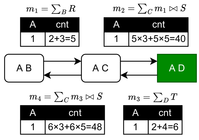
(a) Upward and downward message passing.

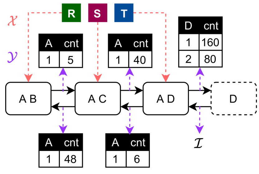
(b) Calibrated Junction Hypertree.

Figure 6. Message Passing and Calibration. Green rectangle is the root. Dotted one is the empty bag. $\mathcal{I}$ is identity relation. $\mathcal{X}$ maps relations to bags, and $\mathcal{Y}$ maps edges to messages.

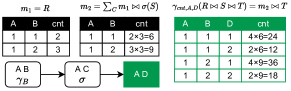
Figure 7. Filter-group-by query with annotated JT.

3.3. Message Passing Over Annotated Bags

We now describe support for general SPJA queries over JT. Although each query JT has the same structure, we annotate the bags based on the query’s SPJA operations. We then modify message passing rules to accommodate the bag annotations. These annotations will come in handy when determining work-sharing opportunities for a new interactive query given a dashboard query.

Given the database $\textbf{R}=\{R_{1},R_{2},...,R_{n}\}$ and JT $=((E,V),\mathcal{X},\mathcal{Y})$, we focus on semi-ring SPJA queries of the following form:
SELECT $\mathcal{G}$, COUNT(*) FROM $\mathcal{J}$
WHERE [JOIN COND] AND $\mathcal{P}$ GROUP BY $\mathcal{G}$
where $\mathcal{G}$ is the grouping attributes, $\mathcal{J}\subseteq\mathbf{R}$ is the set of relations joined in the FROM clause, and $\mathcal{P}$ is the set of predicates referencing attributes in one bag. Query execution is based on message passing (Section 2). However, the processing of each bag differs based on annotations. We propose 4 annotation types, summarized in Table 1:

• GROUP BY $\mathcal{G}$. For each attribute $A\in\mathcal{G}$, we annotate exactly one bag $u$ that contains this attribute with $\gamma_{A}$. Messages emitted by the annotated bag and all downstream bags do not marginalize out $A$. Since all bags containing $A$ form a connected subtree (running intersection), which bag we annotate does not affect correctness. However, we will later discuss the performance implications of different choices when we use CJT to queries.

• Joined Relations $\mathcal{J}$. The query may not join all relations in the join graph, or the joined relations are updated. For each relation R not included (resp. updated) in the query, we annotate the corresponding bag $u=\mathcal{X}(R)$ with $\overline{R}$ (resp. $R^{*}_{ver.}$). When computing messages from this bag, R will be excluded from $\mathcal{X}^{-1}(u)$ (resp. R will be updated in $\mathcal{X}^{-1}(u)$). We allow only the exclusions of relations that don’t violate JT properties.

• PREDICATES $\mathcal{P}$. Let predicate $\sigma\in\mathcal{P}$ be over attribute $\mathbf{A}$. We choose a bag $u$ such that $\mathbf{A}\subseteq u$, and annotate it with $\sigma_{id}$—the effect is that the predicate filters all messages emitted by $u$. The choice of bag to annotate is important—for a single query, we want to pick a bag far from the root in the spirit of selection push down, whereas to maximize message re-usability, we want to pick the bag near the root. We discuss this trade-off in Section 3.3.4.

3.3.1. Message Passing

We now modify how message passing, generation, and absorption work to take the annotations into account.

Upward Message Passing. Traditional message passing chooses a root bag and traverses edges from leaves to the root. Since JT uses bidirectional edges, we call this "upward message passing". The message $\mathcal{Y}(b{\to}p)$ from bag $b$ to parent $p$ is defined as follows: Let $M(b,p)=\{\mathcal{Y}(i{\to}b)|i{\to}b{\in}E\land i{\not\eq}p\}$ be the set of incoming messages (except from $p$). We join between all relations (updated to the specified versions) in $M(b)$ and $\mathcal{X}^{-1}(b)$, and marginalize out all attributes not in $p$. Given annotations, we exclude relations in $\overline{R}$ from the join, apply predicates $\sigma$ (with appropriate push-down), and exclude attributes in $\gamma$: $\mathcal{Y}(b\to p)=\textstyle\sum_{b-(p\cap b)-\gamma}\sigma(\Join(M(b,p)\cup\mathcal{X}^{-1}(b)-\overline{R}))$. $b$’s message to $p$ is ready iff all its messages from child bags are received. During message passing, if $b$ contains group-by annotation $\gamma$, we temporarily annotate all its downstream bags also with $\gamma$.

Absorption. Absorption is when the root bag $r$ consumes all incoming messages. It is identical to the join and filter during message generation: $Absorption(r){=}\sigma(\Join(M(r,\varnothing)\cup\mathcal{X}^{-1}(r)-\overline{R}))$. To generate the final results, we marginalize away all attributes not in $\mathcal{G}$.

Example 8.

Consider database and JT in Figure 2. Suppose we want to query the total count filter by C = 1 and group by B. This requires us to annotate bag AB with $\gamma_{B}$ and bag AC with $\sigma$ (id is omitted). Figure 7 shows the upward message passing over the annotated JT to root AD, where attribute B is not marginalized out and the predicate $C{=}1$ is applied to S. After upward message passing, bag AD performs absorption and marginalizes out AD to answer the query.

3.3.2. Runtime Complexity

The main purpose of this runtime complexity analysis is to serve as a baseline for analyzing the runtime benefits of the CJT in Section 3.4.3. Our analysis largely follows FAQ (abo2016faq, ), with extensions to consider the effects of selection (by selectivity) and group-by (by attribute domain size) annotations. While FAQ also supports group-by, it’s by modifying variable elimination to construct a new JT, and bounding JT by relation sizes. We first use an example to contrast the difference:

Example 9.

Consider relations $R(A,B),S(A,C)$ with a JT of $(AB)-(AC)$; each relation and attribute domain size is $O(n)$ and $O(d)$ respectively. For the query $\gamma_{B,C,count(*)}(R\Join S)$, Treant annotates $(AB)$ with $\gamma_{B}$ and $(AC)$ with $\gamma_{C}$, leading to a JT of $(AB\gamma_{B})-(AC\gamma_{C})$. If $(AC)$ is the root, the absorption of $(AC)$ is bounded by $O(nd)$ (increased by $O(d)$ for $\gamma_{B}$). But in FAQ, this is viewed as variable elimination of only $A$, leading to JT of a single bag $(ABC)$ with absorption size $O(n^{2})$.

Our extension offers two benefits: (1) it improves message reuse as compared to running variable elimination to construct a new JT, and (2) dashboards typically have few group-by attributes with domain sizes much smaller than relation sizes, which improve the bounds. Next, we lay out the setting for our analysis:

• Measure: We measure complexity in terms of both the query and database sizes using the standard RAM model of computation.

• Query: We focus on a SPJA query over an acyclic natural join of $n$ relations $R_{1},...,R_{n}$ with attribute domains of size $O(d)$. The selections and group-bys have been annotated in JT (below).

• Annotated JT: Let the annotated $\texttt{JT}(E,V,\mathcal{X},\mathcal{Y})$ over $n$ bags be the SPJA query. Each bag maps to exactly one relation, whose schema is the same as bag attributes. To simplify notation, we denote the relation of bag $u$ as $R_{u}=\mathcal{X}^{-1}(u)$. For annotations:

  • Selection: $s(u)$ denotes the combined selectivity of all $\sigma$ on $u$.

  • Group-by: $g(u,v)$ denotes the number of attributes to group-by from the upstream bags to $u\to v$ (excluding the group-bys in $u$). Note that the $\sum$ annotations can cancel out the corresponding group-bys and are not counted in $g(u,v)$.

  • Update: We assume $R_{u}$ references the latest relation.

  • Exclusion: While relation exclusion is common for multi-relation bag (e.g., for graph analytics (robinson2015graph, )), it’s rare for single-relation bag, and may lead to disconnected join graph, Cartesian products, and size blowup (except for leaf bag). For simplicity, we assume no relation exclusion.

• Query Execution: Following FAQ (abo2016faq, ), we analyze the WCO LeapFrog Triejoin (veldhuizen2012leapfrog, ). Given a natural join of $n$ relations, $m$ unique attributes, maximum input relation size $N$, and the fractional edge cover bound (atserias2008size, ) of join size $\rho$ (based on the join graph and relation sizes), the runtime complexity is $O(mn{\cdot}\rho{\cdot}logN)$. For SPJA, we pre-apply selection, join, and use standard hash-based aggregation in $O(\rho)$; join dominates the aggregation cost.

Proposition 1 (Runtime Complexity).

Executing SPJA query naively takes $O(|V|\cdot|\cup_{v\in V}v|\cdot\rho\,log(max_{v\in V}s(v)\cdot|R_{v}|)+\sum_{v\in V}|R_{v}|)$, where $\rho$ is the fractional edge cover bound of join size over selected relations. For message passing over JT, given root $r\in V$, define $Tra(r,\texttt{JT})$ as the set of pairs $(u,v)$ for all directed edges $u{\to}v$ on the path to $r$ in $E$. The complexity is then $O(\textstyle\sum_{u,v\in Tra(r,\texttt{JT})\cup\{(r,\varnothing)\}}\mathcal{M}(u,v)+|R_{u}|)$, where $\mathcal{M}(u,v){=}(|U(u,v)|+1)(|u|+g(u,v))\mathcal{S}(u,v)\,log\,max(max_{x\in U(u,v)}\mathcal{S}(x,u),\\ s(u)|R_{u}|)$ is the message passing ($u{\to}v$) cost, $U(b,p)=\{i|i{\to}b\in E\land i\not\eq p\}$ is the set of $b^{\prime}s$ neighbour bags (except $p$) and $\mathcal{S}(u,v)=d^{g(u,v)}s(u)|R_{u}|$ is the size bound of message from $u$ to $v$.

Proof Sketch 0.

The naive SPJA query execution runtime complexity is the sum of leapfrog triejoin and selection cost (in $O(\sum_{v\in V}|R_{v}|)$). Message passing analysis is similar with one difference: messages are aggregated results. This allows us to bound the join output sizes by the domain size of group-by attributes. For each message $u\to v$, we join $u$ with all its incoming messages and aggregate; the cost is dominated by the join. Without group-by annotation, the join size is bounded by $O(s(u)|R_{u}|)$. With group-by annotations, the join (and message) size increases by a factor of the group-by attributes’ domain size $O(d^{g(u,v)})$ Absorption for $r$ follows the same analysis. The final complexity sums selection, message passing, and absorption.

Beside the polynomial difference in query complexity, join sizes are the core difference in data complexity: naive query execution materializes joins ($O(\rho)$), which can be prohibitive. In contrast, factorized execution restricts the join size to $d^{g(u,v)}s(u)|R_{u}|$ for each message passing $u\to v$, which in practice is much smaller.

3.3.3. Single-query Optimization.

For a given SPJA query, we can choose different bags to annotate, and different roots for upward message passing. We make these choices based on heuristics that minimize the runtime complexity. Since relation removal and update annotations $\overline{R},R^{*}_{ver.}$ can be only placed on $\mathcal{X}(R)$, and the placement of group-by don’t affect the message passing, the only factor is the choice of root bag and selection annotations. We enumerate every possible root bag, greedily push down selections, and choose the root with the smallest complexity; the total time complexity to find the root is polynomial in the number of bags.

3.3.4. Message Reuse Across Queries

Messages reuse between queries requires that the message along edge $u\to v$ only depends on the annotated sub-tree rooted at $u$. Thus, a new query can reuse materialized messages in CJT that have the same subtree (and annotations).

Proposition 2 (Message Reusability).

Given a JT and annotations for two queries, consider the directed edge $u\to v$ present in both queries. Let $T_{u}$ be the subtree rooted at $u$. If the annotations for $T_{u}$ are the same for both queries, then the message along $u\to v$ will be identical irrespective of the traversal order nor choice of the root.

This proposition is well established in PGM (shafer1990probability, ), and follows for message passing over JT. The proof sketch is as follows: leaf nodes send messages that only depend on outgoing edges, base relations and annotations, while a given bag’s outgoing message only depends on its mapped relations ($\mathcal{X}$), annotations and incoming messages. None of these depend on the traversal order nor the root.

2 implies that an annotation can “block” reuse along all of its downstream messages. For group-by annotation, we greedily push down it to the leaf of the connected subtree closest to the root to maximize reusability. However, pushing selections down trades-offs potentially smaller message sizes for limited reusability; we discuss this interesting optimization problem in Appendix C.

3.4. Calibration

We saw above that message reuse depends on choosing a good root for message passing, however upward message passing only materializes messages for a single root. Calibration materializes messages for all roots, letting future queries pick arbitrary roots.

3.4.1. Calibration

Given an edge $u\to v$, $u$ and $v$ are calibrated iff their marginal absorption results are the same in both directions: $\sum_{u-(v\cap u)}Absorption(u)=\sum_{v-(v\cap u)}Absorption(v)$. The JT is calibrated if all pairs of adjacent bags are calibrated. We call this a Calibrated Junction Hypertree (CJT), which is achieved by Downward Message Passing discussed next.

Downward Message Passing. Upward message passing computes messages along half of the edges from leaves to root. Downward Message Passing simply reverses the edges and passes messages from the root (now the leaf) to the leaves (now all roots). Now, all directed edges store materialized messages.

Example 10.

Consider the example in Figure 6(a). During upward message passing, root $AD$ receives the message from leaf $AB$. After that, we send messages back from $AD$ to $AB$. We can verify that the JT is calibrated by checking the equality between the absorptions.

Calibration means all bags are ready for absorption. This immediately accelerates the class of queries that furthers adds one grouping or filtering over attribute $A$. We simply pick a bag containing $A$ and apply the filter/group-by to its absorption result.

3.4.2. Query Execution Over a CJT

How do we execute a new interactive query $Q$ over the CJT of a dashboard query $Q_{p}$? Since they share the same JT structure, they only differ in their annotations. The main idea is that query execution is limited to the subtree where the annotated bags differ between the two queries, while we can reuse messages for all other bags in the CJT.

Let ${\bf A_{p}}$ and ${\bf A}$ be the set of annotations for $Q_{p}$ and $Q$, respectively; note that the annotations in ${\bf A_{p}}$ are bound to specific bags in the CJT, while the annotations in ${\bf A}$ are not yet bound. Further, let ${\bf B_{\Delta}}$ be the subset of bags whose annotations differ between the two queries. The minimal Steiner tree $T$ is the subtree in the CJT that connects all bags in ${\bf B_{\Delta}}$ using the least number of bags. Owing to the simplicity of tree structure, the minimal Steiner tree for a specified set of ${\bf B_{\Delta}}$ can be identified efficiently. From 2, edges that cross into $T$ have the same messages as in the CJT and can be reused. Thus, we can only perform upward message passing inside of $T$. Let us first start with an illustrative example:

Example 11 (Steiner Tree).

In Figure 8, the dashboard query $Q_{p}$ groups by D and filters by $B=1$, and so its annotations are ${\bf A_{p}}$ $=\{\sigma_{1},\gamma_{D}\}$. Suppose query $Q$ (row 2) instead groups by A and filters by $C=1$ (${\bf A}$ $=\{\sigma_{2},\gamma_{A}\}$), and we place its annotations $\sigma_{2}$ and $\gamma_{A}$ on AC. The two queries differ in bags ${\bf B_{\Delta}}$ =$\{BC,AC,DE\}$, and we have colored their Steiner tree. Therefore, we can reuse the message $BF\to BC$, but otherwise re-run the upward message passing along the Steiner tree.

Although the example allows us to reuse one message, it’s sub-optimal because ${\bf B_{\Delta}}$ can be further compressed, and the root is poorly chosen. Instead, we use a greedy procedure: we arbitrarily place the annotations on valid bags to create an initial Steiner tree, and then greedily shrink it. Given the minimal Steiner tree over shrinked the ${\bf B_{\Delta}}$, we find the optimal root following Section 3.3.

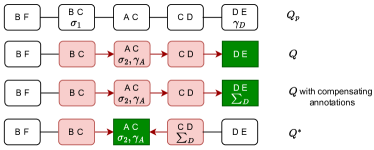
Figure 8. Given CJT of $Q_{p}$, the Steiner tree to execute $Q$ is highlighted (green is root and red is non-root nodes). Compensating annotation $\sum_{D}$ is introduced to compensate $\gamma_{D}$, and can be moved for better plan. $Q^{*}$ is the optimal query with minimum Steiner tree size and runtime complexity.

Initialization. For annotations only in ${\bf A}$, they are added to $Q$’s JT based on the single-query optimization rules in Section 3.3. For annotations only in ${\bf A_{p}}$, we need to compensate for their effects. For $\sigma_{p}$ and $\overline{R}$, we remove the annotation, while for $\gamma_{D}$, we introduce the compensating annotation $\sum_{D}$, which marginalizes out $D$, and place it on the same bag. A unique property of $\sum_{D}$ is that we can freely place it on any bag that contains $D$. For all of the above annotations, we add their bags to ${\bf B_{\Delta}}$. This defines the initial Steiner tree:

Example 12.

The third row in Figure 8 adds the compensating annotation $\sum_{D}$ to DE. Its execution is as follows: BC doesn’t apply $B=1$, AC applies $C=1$, groups by $A$, and DE maginalizes out $D,E$.

Shrinking. Given the leaves of the Steiner tree, we try to move the differed annotations of $Q$ toward the interior of the tree. Recall that $\sigma$, $\gamma$, and $\sum$ can be placed on any bag containing the annotation’s attribute. We greedily choose the bag with the largest underlying relation and move its annotations first to reduce the Steiner tree.

Example 13.

$Q^{*}$ in Figure 8 shows the optimal execution plan over the minimal Steiner tree for $Q$. It has moved $\sum_{D}$ to CD, and made AC the root. CD will marginalize out D, and AC performs the filter and group-by. In this way, we also reuse the message $\texttt{DE}\to\texttt{CD}$.

3.4.3. Runtime Benefit.

After optimization, the query execution runtime complexity with CJT is primarily dictated by the difference between the current query and the CJT, as measured by the size of the Steiner tree, and is never worse than naive execution without the CJT. The proof sketch is as follows: Consider naive query execution over $\texttt{JT}(E,V,\mathcal{X},\mathcal{Y})$ with root $r$. With CJT, we can share the message outside the Steiner tree $\texttt{ST}(E^{\prime}\subseteq E,V^{\prime}\subseteq V)$. We analyze the simple case of message passing over CJT with the original annotation placements without shrinking and the same root choice $r$, which is sufficient to show the runtime benefit; better root choices and shrinking can further improve the time complexity. Let $r^{\prime}=r$ if $r\in V^{\prime}$; otherwise, $r^{\prime}$ is the bag $\in V^{\prime}$ closest to $r$. The runtime complexity for query execution with CJT with root $r$ becomes:

$$O(\textstyle\sum_{u,v\in(Tra(r,\texttt{JT})\cup\{(r,\varnothing)\}){\color[rgb]{1,0,0}\setminus(Tra(r^{\prime},\texttt{JT})\setminus Tra(r^{\prime},\texttt{ST}))}}\mathcal{M}(u,v)+|R_{u}|)$$

The core benefit of CJT is to enable the sharing of messages highlighted in red. These messages have all upstream bags outside of ST, whose annotations are thus the same. They can therefore be shared according to 2. As we can see, similar queries require fewer annotations, and thus a smaller Steiner tree that requires the same or fewer messages. The benefits are particularly pronounced for imbalanced relation sizes, such as a snowflake schema, where changes are in the small dimension tables. Messages from the fact table can be shared to avoid joining and aggregating the fact table.

Applying CJT to Dashboard and Challenge. CJT is highly suitable for the interactive dashboard: Offline, we build CJT for dashboard query. Online, given interaction query, CJT ensures that computation needed is proportional to the difference between it and dashboard query (Steiner tree); such a difference is generally small, thanks to the incremental nature of the dashboard interactions. However, one challenge arises when users submit multiple interaction queries, each building upon the previous one. As the number of iterations increases, the Steiner tree is likely to expand due to the growing differences. Ideally, we would want to calibrate not only dashboard query but also interaction queries. However, interaction queries are only available online; calibrating them will slow down user interactions. In the next section, we present an optimization to hide such a slowdown. The insight is that users typically have "think-times" (eichmann2020idebench, ) during interactions; we leverage it to calibrate interaction queries in the background without affecting users.

4. System Overview

In this section, we provide the overview of Treant, a dashboard accelerator that manages CJT to support interactive queries over join. We discuss Treant’s usage, architecture, and optimizations.

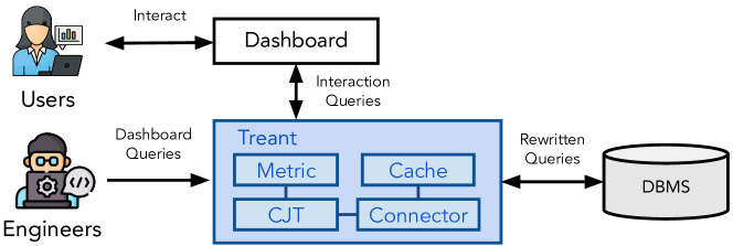
Figure 9. Treant architecture.

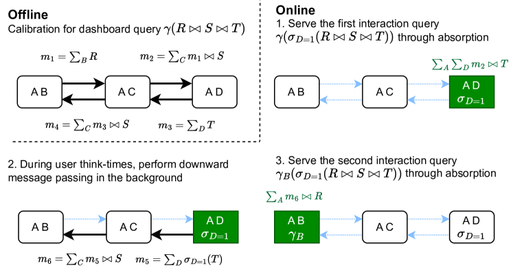
Figure 10. Example CJT management by Treant.

4.1. Usage Walkthrough

We describe the detailed process of using Treant to build and use an interactive dashboard. Treant has both offline and online stages.

4.1.1. Offline Stage.

The engineering team gathers data and constructs the dashboard offline through the following steps:

Define Metrics. Different domain users have different metrics of interest. For example, the sales department is interested in revenue, while the marketing department is interested in return on investment (ROI). The engineering team defines them as semi-ring aggregation (Section 2) which express a wide range of aggregations.

Construct Join Graph. In enterprise data warehouses, there are typically a large number of tables for metrics and enrichment dimensions (join). The engineering team constructs a join graph that specifies these tables and the join conditions.

Build Visualization. The engineering team specifies the visualizations in the dashboard. Each visualization encodes data from a dashboard query. For instance, a bar chart encodes a dashboard query with one group-by, while a heatmap encodes one with two group-bys. Treant provides basic visualizations for the dashboard, but is also compatible with any external visualization system.

Finally, Treant takes as input the dashboard queries (with metrics as semi-ring aggregations and join graphs in join clauses), connects to DBMS and pre-processes them for future dashboard interactions.

4.1.2. Online Stage.

Domain users navigate dashboard to analyze metrics of interest. They interact with the dashboard through widgets, which in turn trigger interaction queries that modify the initial dashboard query. For example, a drop-down menu can modify the group-by attribute, while a slider can change the selected month of the dashboard query. Treant supports interaction queries that:

• modify select/group clause of the dashboard query (Section 3.3)

• update or remove table in the join clause (Section 3.3)

• join with new table that create/affect one bag (Section 4.3)

4.2. Architecture

We first describe how Treant manages CJT for the interactive dashboard, and then delve into the internal components.

4.2.1. Management of CJTs.

Treant manages CJTs for work sharing between dashboard queries and interaction queries. Treant first builds CJTs for dashboard queries offline to accelerate interaction query online. However, users are likely to engage in more interactions that incrementally modify the previous interaction query. Treant further calibrates interaction query online: for each visualization (dashboard query) and user session, Treant builds CJT for the latest interaction query during users’ "think-times" (eichmann2020idebench, ) in the background. Note that the calibration doesn’t need to be complete and is halted on receiving the next interaction query to not degrade interactivity. Treant can use the partially finished CJT and take advantage of the finished messages to speed up interaction query.

Example 14.

We illustrate the CJT management using the example join graph (Figure 2(b)) in Figure 10. Given a visualization of a single number with dashboard query $Q_{1}=\gamma(R\Join S\Join T)$, Treant builds its CJT offline. During online phase, user interact with the dashboard with interaction query $Q_{2}=\gamma(\sigma_{D_{1}}(R\Join S\Join T))$, and Treant uses $Q_{1}$’s CJT to share messages. During user think-times, Treant calibrates $Q_{2}$ in the background. User performs the next interaction with interaction query $Q_{3}=\gamma_{B}(\sigma_{D_{1}}(R\Join S\Join T))$, and Treant uses $Q_{2}$’s CJT.

4.2.2. Internal Components.

Treant internals are shown in Figure 9. In contrast to previous factorized systems (khamis2018ac, ; schleich2019layered, ) that use custom engines, Treant is a middleware that sits between the dashboard and users’ DBMSes. It takes a dashboard query or interaction query as input, applies pure query rewriting, uses CJT to determine the necessary messages to be computed, and computes messages by issuing SPJA queries to DBMSes. This makes Treant portable to any DBMS that executes SPJA queries. The contents of messages (SPJA query results) are stored as tables in the DBMS and Treant stores the pointers (table names) to these messages.

Offline, Treant establishes a connection to DBMS through connectors. For each visualization, the data engineer specifies its dashboard query (with semi-ring aggregation) and Treant stores it in the metric component. Then, Treant re-writes dashboard query for message passing and builds CJT to pre-compute messages.

Online, Treant takes an interaction query as input, finds the corresponding CJT of previous interaction query (LABEL:{sec:cjtmanage}) based on the user session and the visualization, if available, or uses the dashboard query otherwise. Then Treant uses that CJT to pass messages only within the Steiner tree (Section 3.4.2), performs absorption, retrieves the results and sends them to the dashboard for visualizations. The created messages are similarly stored within the DBMS, and only the pointers are returned. In the background, Treant further calibrates interaction query (LABEL:{sec:cjtmanage})

Finally, while the focus of Treant is to share messages from the most recent CJT (the current dashboard state) for single-user session, there can be work-sharing opportunities from (1) prior partially calibrated JT and (2) CJT across user sessions. At present, Treant takes advantage of these opportunities through a message-level cache: For each message, Treant encodes its query definitions and the upstream sub-tree of the messages as the cache key (adequate to uniquely identify the message as per 2), with the message pointer as value. Before sending a message query to the DBMS, Treant checks if the message is cached. The cache utilizes an LRU replacement policy by default, but refrains from removing messages if they are referenced by CJTs from dashboard query or active user sessions. Upon removal of a message from the cache, Treant submits a deletion query for the message to the DBMS.

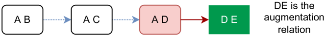
Figure 11. Augmenting the join graph with DE. The Steiner tree is AD $\rightarrow$ DE with root DE and requires one message (red).

4.3. Augmentation Optimization

Simple ML models like linear regression are widely used to examine attribute relationships in the dashboard (morton2012trends, ). Data and feature augmentation (chepurko2020arda, ) further identify datasets to join with an existing training corpus in order to provide more informative features, and is a promising application on top of data warehouses and markets (fernandez2020data, ; chepurko2020arda, ; fernandez2018aurum, ). However, the major bottleneck is the cost of joining each augmentation dataset and then retraining the ML model.

The SOTA factorized ML (nikolic2018incremental, ; schleich2016learning, ; schleich2019layered, ; curtin2020rk, ) avoids join materialization when training models over join graphs. First, it designs semi-ring structures for common models (linear regression (schleich2016learning, ), factorization machines (schleich2021structure, ), k-means (curtin2020rk, )), and then performs upward message passing through the join graph. If we augment with relation $r$, then factorized learning approaches execute the message passing through the whole augmented join graph again.

In contrast, CJT allows us to choose any bag $b$ that contains the join keys, construct an edge $b\to r$, and perform message passing using $r$ as the root. In this setting, the Steiner tree is exactly 2 bags, and the rest of the messages in the CJT can be reused. For instance, Figure 11 shows a join graph $\texttt{AB}\to\texttt{AC}\to\texttt{AD}$ that we augment with DE. The Steiner tree is simply AD and DE, and we only need to send one message to compute the updated ML model.

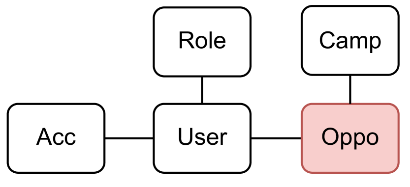
(a) Salesforce

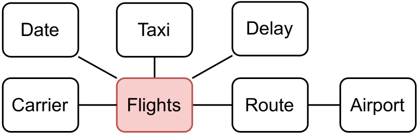
(b) Flight

Figure 12. Database schema. Red relation is the largest.

4.4. Limitations and Future Works

The focus of this paper is on the message sharing opportunities, demonstrated through a simplified class of SPJA queries. There are limitations in the types of queries currently supported, and we aim to enhance expressiveness in future work to broaden applicability.

Limitations. The current implementation uses parameterized SPJA based on exact matches, as per the format in Section 3.3 and does not parse general SQL strings that can be rewritten to match this format. In terms of expressiveness, Treant supports predicates over only attributes in a single bag for selection; for a predicate clause that references attributes from different bags (e.g., $T.a=R.b$), Treant treats it as a post-processing of group-bys, which could be inefficient. Selection over aggregate query results is unsupported. For aggregation, Treant only supports semi-ring aggregations; while semi-ring can express almost all commonly used aggregations, percentile-based (e.g., median), and distinct-based (e.g., distinct count) aggregates are not supported. As for augmentation, Treant currently allows changes that create or affect a single bag; augmentations with attributes spanning across multiple bags are not permitted. Beyond SPJA queries, Treant supports ORDER BY and LIMIT, but as a naive post-processing over the SPJA query result that’s not optimized.

Future works. We aim to support semantically equivalent rewrites using existing methods like SPES (zhou2019automated, ). For selections that reference attributes spanning multiple bags, recent optimization (khamis2020functional, ) can be applied to build range searching data structure for inequality predicates. For predicate that references results from other SPJA queries, a hierarchical CJT (wu2007hierarchical, ) that references other CJTs is a prospective direction. For percentile-based aggregations, we plan to apply semi-ring approximations (cormode2011sketch, ). Dealing with augmentations where join keys span multiple bags is another challenge we hope to address, as discussed in Appendix B. For ORDER BY and LIMIT, we plan to integrate TOP-N optimizations (donjerkovic1999probabilistic, ) and approximations from MAP (wainwright2005map, ; conaty2017approximation, ) with Treant.

5. Experiments

Can Treant support interaction queries at interactive speeds? What is the overhead? How well can Treant handle more complex applications like ML augmentation? We conducted experiments on both a single node DBMS (DuckDB (raasveldt2019duckdb, )) and a cloud DBMS (Redshift).

5.1. Single-node DBMS Experiments

Our single-node DBMS experiments are designed to emulate the settings of local processing on a laptop. We evaluate Treant on DuckDB (raasveldt2019duckdb, ) due to its popularity: DuckDB is an OLAP DBMS with superior single-node performance and seamless integration with other Python/R data analytics libraries.

Setup. We use two datasets for dashboards: Salesforce(salesforce, ), a public dataset provided by Sigma Computing for CRM and marketing analysis with 36 numerical and 229 categorical attributes; and Flight(flight, ), a real-world dataset with 27 numerical and 5 categorical attributes, commonly used in interactive data exploration (eichmann2020idebench, ). However, Salesforce is a demo dataset of only $27MB$, while modern laptop can process $>10GB$ data with DuckDB. To address this discrepancy, we employ the data scaler in IDEBench (abourezq2016database, ) to scale both datasets. The scaling process involves denormalization, estimating the distribution, sampling rows from the distribution, and finally normalizing the table through vertical partitioning. We scale Salesforce to 50M rows for 13.7GB, and Flight for 300M rows for 15GB. The final normalized schemas are in Figure 12.

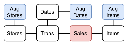
Figure 17. Favorita schema. Sales is the largest relation. Aug Stores, Aug Dates and Aug Items are augmentation relations.

For ML augmentation, we use the Favorita (favorita, ) dataset of purchasing and sales forecasts, widely used in prior factorized ML (schleich2016learning, ; schleich2019layered, ) (see Figure 17 for the schema). Sales is the largest relation (241MB), while the others are $<2MB$. All experiments were run on GCP c2d-standard-4 (4 vCPUs, 16 GB RAM).

5.1.1. Salesforce Dashboard

We conduct experiments on the Salesforce dashboard (salesforce, ) built by Sigma Computing.

Workloads. The Salesforce dashboard tracks various metrics such as pipeline, and productivity, which are all computed using the sum aggregations. However, we find that the specific metric chosen has little impact on the query performance. Therefore, we randomly choose the total pipeline amounts as the metric.

We consider two types of visualizations from the Salesforce dashboard illustrated in Figure 1(b): a single value visualization, which corresponds to a dashboard query without group-by or selection, and a pie chart that is grouped by Campaign (Camp) type. The dashboard includes drop-down lists for selecting the user name, title, campaign start date, role name, and group-by user title or account state; we experiment with all of these interactions. We further conduct tests of interactions that modify the Camp relation (by random cell value perturbations) and remove the Acc relation.

Baselines. We consider the following baselines

• Naive: Execute the naive SPJA queries translated from dashboard interactions in the DBMS without implementing factorized query execution nor work-sharing from pre-computed data structures.

• Factorized: Rewrite the naive queries into message passing for factorized execution, but still doesn’t exploit work-sharing.

• Treant consists of multiple stages for online interaction query execution (directly experienced by the users) and the offline/background calibration overheads. We report them separately:

  • Treant: online interaction query execution using CJTs (from prior interaction query or dashboard query) for acceleration.

  • CalibrateOffline: offline calibration overhead to construct CJTs for the initial dashboard queries.

  • CalibrateOnline: background calibration overhead to construct CJT for the current interaction query (to proactively expedite future queries), which doesn’t need full completion.

Results. Figure 13 presents the results. The performance of both Factorized and Naive varies depending on the type of interaction, with faster performance for selection due to smaller data sizes to process. However, they still take $>2s$ for most interaction queries and can be as slow as $7s$. We find that factorized execution (Factorized) alone results in even slower performance than Naive. This is because Factorized is optimized for many-to-many joins, which are not present in Salesforce workloads. Additionally, Factorized introduces additional aggregations for each join edge.

In contrast, Treant is able to execute various types of interaction queries, from selection, group-by, to relation update and removal, within $100ms$ by reusing messages, offering two orders of magnitude improvements; the offline overhead (CalibrationOffline) is only ${\sim}2\times$ the cost of executing the dashboard query by Factorized. To ensure quick responses in future interactions, Treant calibrates interaction query (CalibrationOnline) whose time is at the same scale as Factorized as it only requires downward message passing (Section 3.4), and is well within user think-times (${<}10s$ (eichmann2020idebench, )). Furthermore, CalibrationOnline is in the background during user think-times, and doesn’t require full completion. Regarding storage, the intermediate messages only occupy $363MB$ ($<3\%$ of DB size).

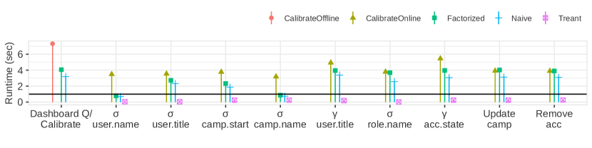
(a) Performance for single value visualization.

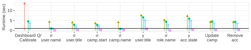
(b) Performance for pie chart grouped by Campaign Type.

Figure 13. Salesforce Dashboard Performance. Horizontal line shows the $1s$ interactive response threshold.

5.1.2. Flight Dashboard

We next experiment with the Flight dataset (flight, ).

Workloads. IDEBench (eichmann2020idebench, ) produces a random workload consisting of a collection of visualizations (dashboard queries) and, for each visualization, a series of interaction queries that progressively incorporate selections. We use the default workload, which contains 8 total interaction queries across 5 visualizations. We use the same baselines as in Section 5.1.1. However, to demonstrate the advantage of online calibration, we evaluate Tre+Offline, which only uses CJTs created offline. Based on IDEBench recommendation, we use a think-time of $10$s by default, and study the sensitivity later.

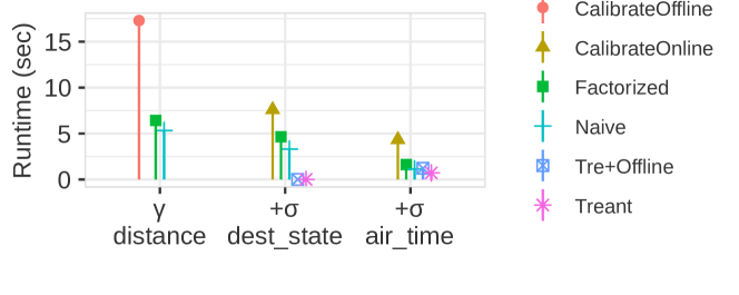
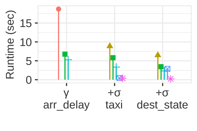
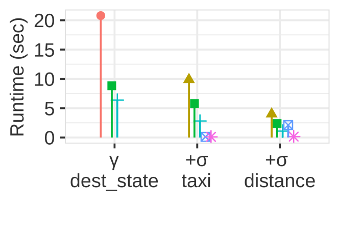
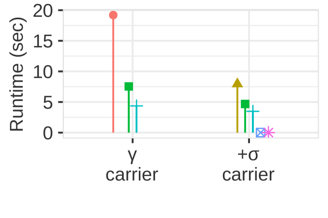
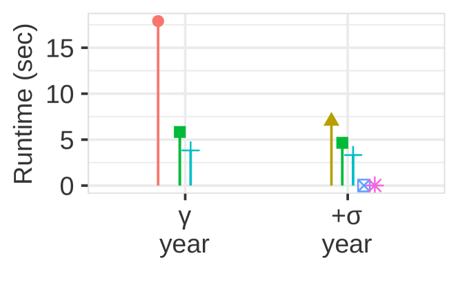
Figure 14. Flights Dashboard Performance. The dashboard features five visualizations. For each visualization, the leftmost is dashboard query. interaction queries progressively adds ($+$) selection or group-by element to the previous one.

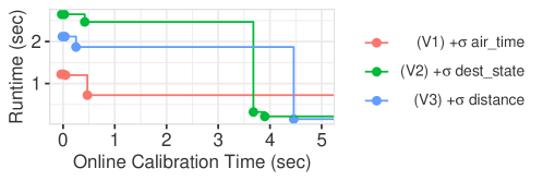
Figure 15. Runtime for the second interaction query over the first three visualizations, with varying online calibration.

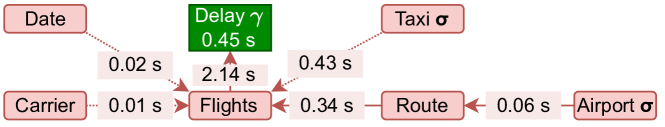
(a) Factorized performs message passing without sharing.

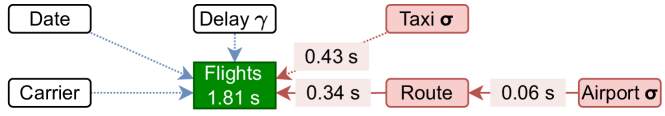
(b) Tre+Offline shares messages, but only with offline CJT.

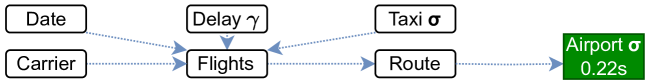
(c) Treant enhances message sharing via online calibration.

Figure 16. Case study for the second interaction query over the second visualization. Blue dotted lines represent shared messages, while red lines indicate computed messages with respective runtimes noted on the edges. The absorption runtimes are displayed in the green rectangle bag.

Results. The results are displayed in Figure 14. Both Factorized and Naive take $3{-}6s$ for most queries. For Treant, offline calibration is ${\sim}3\times$ Factorized due to the larger message size during the group-bys, but reduces Treant to ${<}200ms$. Online calibration takes $4-9s$, well within the think-time of $10s$. For the second interaction queries of the $2^{nd}$ and $3^{rd}$ visualizations, using only offline-created CJT (Tre+Offline) takes $>2s$ due to the larger Steiner tree size, and online calibration reduces this time by ${>}10\times$. In terms of storage, the intermediate messages take up just $89MB$ ($<1\%$ of DB size).

Online Calibration Sensitivity. For online calibration, think-time may not always be possible to leverage. For instance, in multi-tenant DBMS, other users may execute their queries concurrently while one user is thinking. To examine this, we study the second interaction query in the first three visualizations, whose runtime depends on the online calibration. Figure 15 presents the interaction query runtime with varying online calibration time. The plot shows a stepped pattern, as reductions in interaction query runtime only occur upon completion of sharable message computations. Consequently, each step corresponds to a completed sharable message. Without online calibration, the runtime equals that of Tre+Offline. As online calibration time increases, the runtime decreases accordingly due to partial calibration, and reaches ${<}1s$ after only ${<}5s$.

Case Study. To understand where the performance improvements stem from, we conduct a case study on the second interaction query over the second visualization, because it shows the most significant improvement. Figure 16 shows the detailed runtime for each message and absorption for different baselines. Factorized performs message passing without sharing, while Tre+Offline shares messages but only with the offline CJT. They are slowed by the costly message passing or absorption over the large fact table (${>}1.8s$). In contrast, Treant greatly improves message sharing using online calibration. Once the online calibration is completed, the JT is calibrated. For the interaction that selects Airport attribute, this only requires an absorption over Airport (small dimension table) in $0.22s$.

5.1.3. ML augmentation

We next evaluate the benefit of Treant for ML augmentation using the Favorita dataset.

Workloads. We train linear regression using (Sales.unit_sales,
Stores.type, Items.perishable) as features, and Trans.transactions (number of transactions per store, date) as the target variable $Y$.

To simulate a data warehouse with augmentation data of varying effectiveness, we generate synthetic data to augment (join) with Dates, Stores, and Items. For each of these three relations, we first generate a predictive feature $\hat{Y}$ as the average of Y grouped by primary key. We then create 10 augmentation relations with schema (k,v), where k is the primary key and v varies in correlation $\hat{Y}$ (kaiser1962sample, ): The correlation coefficient $\phi$ is drawn from the inverse exponential distribution $min(1,1/Exp(10))$, and the values are the weighed average between $\hat{Y}$ and a random variable weighed by $\phi$. We individually evaluate the model accuracy ($R2$) for each of the 30 augmentation relations, and measure the cumulative runtimes.

In addition to Treant, we also compare the training time of Fac that applies factorized ML but trains each model independently without work sharing, and LMFAO (schleich2019layered, ), the SOTA factorized ML system that is algorithmically similar to Fac but implemented with a custom engine in C++ and not portable to user DBMSes. To ensure a fair comparison, we exclude the time required to read files from disk and the compilation time for LMFAO, but include all the time needed to build data structures and run queries.

Results. Figure 18(a) reports the cumulative runtime to augment and retrain the model. Fac takes ${>}1.3$ min, while Treant takes ${\sim}6s$: calibration dominates the cost, and is ${\sim}2\times$ the cost of training a single model because of the downward message passing. However, after calibration, Treant evaluates all 30 augmentations in ${<}1s$. LMFAO takes ${\sim}1.3\times$ less time than Fac for model training due to implementation difference, but even when including the offline calibration cost, Treant is ${\sim}13\times$ faster than LMFAO after 30 augmentations. Figure 18(b) reports the accuracy improvement above the baseline ($0.031$) after each augmentation, and we see a wide discrepancy between good and bad augmentations ($+0$ to $+0.61$).

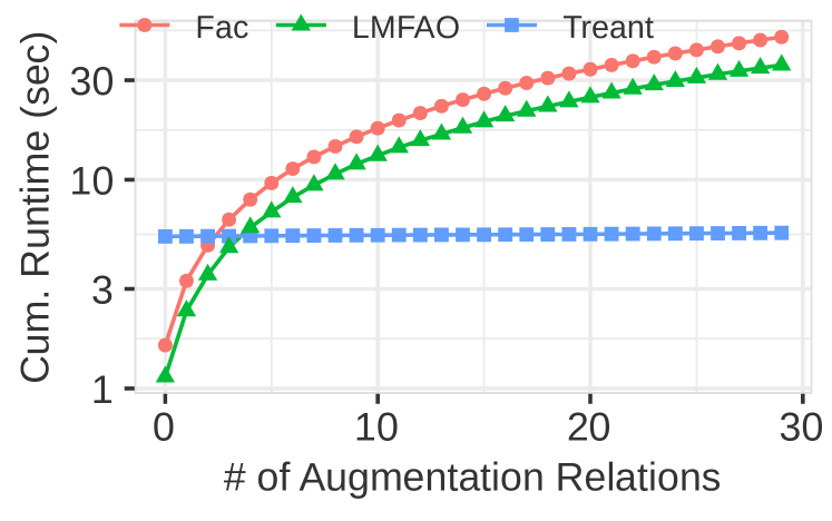
(a) Cumulative runtime (log)

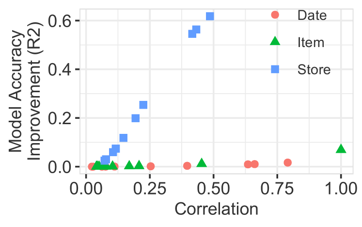
(b) Accuracy (R2) improvements.

Figure 18. Augmentation run time and model performance.

5.2. Cloud DBMS Experiments

We now evaluate Treant on the cloud DBMS (AWS Redshift).

Setup. We use TPC-H (SF=50) for dashboard and TPC-DS (SF=50) for empty bag optimizations. We used dc2.large node (2 vCPU, 15GB memory, 0.16TB SSD, 0.60 GB/s I/O). All experiments warm the cache by pre-executing queries until the runtime stabilizes.

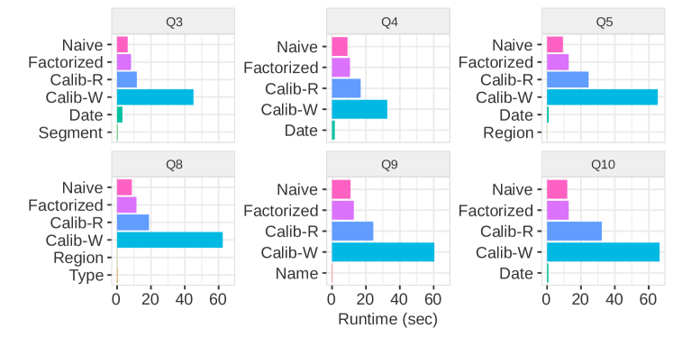
Figure 19. Run time for TPC-H dashboard. Naive executes queries without message passing. Factorized executes queries with message passing. Calib-R computes messages for calibration without materializing them, and Calib-W materializes them. The remaining bars are for interaction queries that vary the values of the parameters (labels).

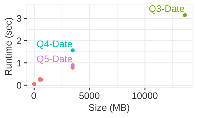
(a)

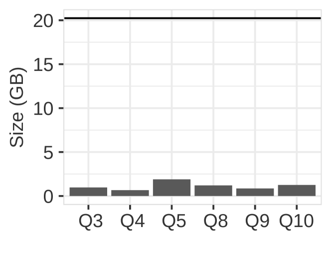
(b)

Figure 20. (a) Size of annotated bag (by predicate) vs query runtime. (b) Total message size overhead of Treant. Horizontal line is the TPC-H database size (${\sim}20$ GB).

5.2.1. Interactive Dashboard

We evaluate Treant on TPC-H queries.

Workloads. We build an interactive dashboard based on a subset of the TPC-H queries (Q3-5,8-10) that can be rewritten as SPJA queries (see Appendix E). These TPC-H queries are parameterized, so we construct a dashboard query for each using random parameter values and then create interaction queries that vary each parameter.

We compared the runtime of the interaction query using different approaches: Naive simply executes the query on Redshift; Factorized rewrites the query as message passing for factorized query execution; and Treant. For Treant, we reported calibration execution cost (Calib-R) separately from the calibration materialization cost (Calib-W), since writes on Redshift are particularly expensive.

Results. Figure 19 shows the run time. Calibration (Calib-W) takes $4{\sim}7\times$ longer than Naive. As expected, upward and downward message passing alone is ${\sim}2\times$ slower (Calib-R), and the rest is dominated by high write overheads; Q8 groups by 2 attributes, so its message sizes are ${\sim}2\times$ larger, and $4\times$ slower overall. As in Section 5.1.1, Factorized is slower than Naive because there is no many-to-many join and it has additional aggregation overheads.

In contrast, Treant accelerates TPC-H queries by nearly $1000\times$ over Naive for parameters including Segment, Region and Type. Naturally, the speedup depends linearly on the size of the bag that contains the parameterized attribute (Figure 20(a)). Q3 Date incurs a higher cost as it includes the fact table in Steiner tree, which could be optimized by creating an empty bag for Date (Section 3.2). We note that the space overhead for calibration is only ${<}2GB$ compared to the original database size ${\sim}20GB$ (Figure 20(b)). This is because messages are aggregated results from these relations.

5.2.2. Empty Bag Optimization

Empty bags are a novel extension to materialize custom views. We evaluate the costs and benefits of empty bags using TPC-DS. We create an empty bag (Store,Time) as illustrated in Figure 5(b). Then, we query the maximum count of sales for all stores and times: ${\bf Q}=\gamma_{MAX(COUNT)}(\gamma_{COUNT(\cdot),Store,Time}(\Join))$ in two unique ways: (1). Without Empty Bag, ${\bf Q}$ is executed by first aggregating the count over the absorption result of Store_Sales, since Store_Sales is the only bag contains both Store and Time dimensions, then computing the max sales. (2). With Empty Bag, ${\bf Q}$ is executed directly over the absorption result of the empty bag, which is sufficient to answer aggregation queries over (Store,Time).

Figure 21 shows the runtimes and sizes. Empty bag takes ${\sim}3s$ to build, and accelerates ${\bf Q}$ by ${\sim}25\times$. Additionally, the storage space required for the empty bag is $21\times$ smaller than that of Store_Sales.

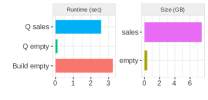
Figure 21. Runtime to build and query the empty bag and Store_Sales table, and their storage sizes.

6. Related Work

Interactive Queries. Previous works use indexing and data cubes (gray1997data, ) to support interactive queries. Some studies have improved them to Nanocubes (lins2013nanocubes, ) for spatiotemporal data and Hashedcubes (pahins2016hashedcubes, ) with additional optimizations, or use sophisticated materialization techniques (liu2013immens, ; moritz2019falcon, ). However, these approaches often have high preprocessing overhead (e.g., taking hours for 200MB data (lins2013nanocubes, )), and require denormalization for large joins. In contrast, CJT has been shown to be exponentially more efficient for interactive queries over large joins (Appendix D) than data cubes with a constant factor overhead.

Early Marginalization. Early Marginalization was first introduced by Gupta et al. (gupta1995aggregate, ) as a generalized projection for simple e.g., count, sum, max queries. It was extended by factorized databases to compactly store relational tables (olteanu2015size, ) and quickly execute semi-ring aggregation queries (schleich2019layered, ; joglekar2015aggregations, ). Abo et al. (abo2016faq, ) generalize early marginalization and establish the equivalence between early marginalization and variable elimination in Probabilistic Graphical Models (koller2009probabilistic, ). However, prior works (schleich2019layered, ) only share work within a query batch but not between batches for interactive queries.

Calibrated Junction Tree. Calibration Junction Tree was first proposed by Shafer and Shenoy (shafer1990probability, ) to compute inference over probabilistic graphical models. While it has found extensive applications across fields such as engineering (zhu2015junction, ; ramirez2009fault, ), ML (braun2016lifted, ; deng2014large, ), and medicine (pineda2015novel, ; lauritzen2003graphical, ), its use has been limited to probabilistic tables (for sum of probabilities). The calibration process is reminiscent of Yannakakis’s two-pass semi-join reduction (yannakakis1981algorithms, ). However, Yannakakis’s algorithm mainly aims to eliminate redundant tuples in individual relations as a pre-processing step for single query execution. Furthermore, it does not materialize messages and is restricted to the 0/1 semi-ring. In contrast, CJT materializes messages for future reuse across queries. In this work, we broaden the scope of CJT to general semi-ring aggregation for SPJA queries.

Semantic Caching. To accelerate online queries, semantic caching (ren2003semantic, ; ahmad2020enhanced, ; chaudhuri1995optimizing, ; gupta1995adapting, ; asgharzadeh2009exact, ) caches previous SPJA query results and reuses them for later SPJA queries, by taking row/column containment, predicate overlaps (theodoratos2004constructing, ; guo1996satisfiability, ), and constraints into account (gupta1995adapting, ; ren2003semantic, ; gryz1998query, ). The analysis for identifying reuse opportunities has also been applied to identify materialized views to reuse (li2005formal, ). In contrast, Treant specifically exploits the semiring properties of the aggregation functions to 1) leverage factorized query execution via message passing, 2) identify partial aggregates (messages) to cache during query execution, and 3) identify the best plan that reuses the cached partial aggregates. Like caching, Treant executes and caches online. In addition, Treant proactively populates the cache in anticipation of incremental changes to the most recently executed query, leveraging user think-time. Treant currently only shares "messages" with identical query definitions and leave other types of sharing (e.g., row/column containment, predicate overlaps) as future works.

Multi-query optimization. Multi-query optimization (MQO) (roy2000efficient, ; hong2009rule, ; schleich2019layered, ) shares the state and computation of subexpressions across queries (e.g., sharing scans across queries). However, it centers on batches of queries known a priori. The optimization of interactive dashboards can be considered as an online version of multi-query optimization. Treant approaches this by applying a practical heuristic that interactive queries are incremental, and uses "messages" as the core unit to reuse. These ideas could be integrated into MQO.

7. Conclusions

We present Treant, a dashboard accelerator over joins. Treant uses factorized query execution for aggregation queries over large joins, and proactively materializes messages, the core intermediates during factorized query execution. that can be shared across interaction queries. To effectively manage and reuse messages, we introduced the novel Calibrated Junction Hypertree (CJT) data structure. CJT uses annotations to support SPJA queries, applies calibration to materialize messages in both directions and computes the Steiner tree to assess the reusability of messages. We implement Treant to manage CJT as middleware between DBMSes and dashboards. Our experiments evaluate Treant on a range of datasets on both single node and cloud DBMSes, and we find that Treant accelerates dashboard interactions by two orders of magnitude.

Appendix A Message Passing Algorithm

Algorithm 1 Message Passing and Calibration Algorithm

1:// Pass Message from bag u to v where $u,v\in V$ 

2:function PassMessage($((E,V),\mathcal{X},\mathcal{Y})$, u, v) 

3:     // All the neighbours 

4:     $N(u)=\{c|c\to u\in\mathcal{E}\}$ 

5:     // All incoming messages from in-neighbours except v 

6:     $M(u)=\{\mathcal{Y}(i\to u)|i\in N(u)\land i\not\eq v\}$ 

7:     // Compute and store message from u to v 

8:     $\mathcal{Y}(u\to v)=\sum_{u-v\cap u}\Join\left(M(u)\cup\mathcal{X}^{-1}(u)\right)$ 

9:end function

10: 

11:// Upward Message Passing to root $r\in V$  

12:function Upward($((E,V),\mathcal{X},\mathcal{Y})$, r)

13:     for all Bag $c\in V-r$ from leaves to root r bottom up do 

14:         p = parent of c 

15:         PassMessage($((E,V),\mathcal{X},\mathcal{Y})$, c, p) 

16:     end for

17:end function

18: 

19:// Downward Message Passing from root $r\in V$  

20:function Downward($((E,V),\mathcal{X},\mathcal{Y})$, r)

21:     for all Bag $p\in V$ from root r to leaves top down do 

22:         for all child bag c of p do 

23:              PassMessage($((E,V),\mathcal{X},\mathcal{Y})$, p, c) 

24:         end for

25:     end for

26:end function

27: 

28:// Calibrate Junction Hypertree  

29:function Calibration($((E,V),\mathcal{X},\mathcal{Y})$)

30:     // choose a random bag as root 

31:     $r\in V$  

32:     Upward($((E,V),\mathcal{X},\mathcal{Y})$, r) 

33:     Downward($((E,V),\mathcal{X},\mathcal{Y})$, r) 

34:end function

Appendix B Feature Augmentation with CJT.

While feature augmentations over single join key are efficient, those over multiples multiple join keys are complex. We need to query the CJT group-by all join keys, which might result in a large Steiner Tree and we need to re-design the JT after augmentation.

Feature Augmentation over Multiple Bag. For Feature Augmentation over multiple, we want to query the aggregation group-by the join keys from CJT. This could be considered as a SPJA query with group-by annotations, and can be computed through Upward Message Passing in the Steiner tree.

Connect Augmentation Relation to JT. To connect augmentation relation to JT where the join key is distributed over multiple bag, we have to add all the join key to the bags of Steiner tree, create an augmentation bag containing augmentation relation, and connect the augmentation bag to any of the bag in Steiner tree. Notice that the JT with added attributes in the bags can be inefficient, and we may redesign JT to find a better one.

Optimize CJT design. To optimize CJT for feature augmentation, we create empty bags for common join keys. Consider TPC-DS as an example, whose (simplified) join graph (also JT) is shown in Figure 5(a). We can cluster time and stores in an empty bag shown in Figure 5(b) to support efficient augmentation of spatio-temporal features.

Appendix C Selection Pushdown.

2 implies that an annotation can “block” reuse along all of its downstream messages. For group-by annotation, we greedily push down it to the leaf of the connected subtree closest to the root to maximize reusability. However, pushing selections down trades-offs potentially smaller message sizes for limited reusability:

Example 15.

Suppose we have materialized messages for $Q_{1}$ in Figure 22, and want to execute $Q_{2}$, which has an additional predicate over C. If we annotated bag BC with $\sigma$, this may reduce the message size but we cannot reuse the message in $\texttt{BC}\to\texttt{CD}$. If we annotate CD ($Q^{\prime}_{2}$), we can reuse the message but risk larger message sizes.

In practice, we prioritize reuse by pulling annotations close to the root—reuse helps avoid scan, join, and aggregation costs, whereas larger message sizes simply increase scan sizes.

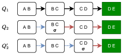
Figure 22. Message size vs reuse trade-off. Given total count query $Q_{1}$, $Q_{2}$ adds a predicate to C. Pushing down selection as in $Q_{2}$ may reduce message size but hinders reuse as compared to $Q^{\prime}_{2}$. Dotted blue edges are reusable messages and solid red edges are non-reusable edges.

Appendix D Data Cube

OLAP data cubes [29] materialize a lattice of data cuboids parameterized by the set of attributes that future queries will filter/group by. Traditionally, the data structure is built bottom-up in order to share computation—each cuboid is built by marginalizing out irrelevant attribute(s) from a descendant cuboid. If the cube is over a join graph, then there is the additional cost of first materializing the (potentially very large) join result to compute the bottom cuboid. Although prior work explored many optimizations (parallelization [79, 20, 73], approximation [76], partial materialization [35, 78], early projection [44]), neither early marginalization nor work-sharing based on CJTs have been explored.

CJTs are a particularly good fit for building data cubes because, in practice, they are restricted to a small number of attributes in order to avoid exponentially large cuboids. In this setting, we can build CJTs for a carefully selected set of pivot queries to accelerate cube construction by 1) not materializing the full join graph when building the cuboids, and 2) aggressively reuse messages to answer OLAP queries not directly materialized by a cuboid.

D.1. Complexity Analysis

Let us first analyze the complexity of using CJTs to answer OLAP queries. This will provide the tools to trade-off between OLAP query performance and space requirements for materialization.

Let the database contain $r$ relations each with $O(n)$ rows, the domain of each attribute is $O(d)$, and the join graph contains $m$ unique attributes. Suppose we have calibrated each cuboid with $k$ group-by attributes (the pivot queries). Calibration costs $O(rnd^{k})$ for each pivot query where the cost per bag is $O(nd^{k})$ (cross product between relation size $n$ and incoming messages). Since the output message size is also bound by $O(nd^{k})$ due to marginalization, we incur this cost for each of $r$ bags in the CJT. Thus the total cost is $O(rn(dm)^{k})$ to calibrate all $\binom{k}{m}=O(m^{k})$ pivot queries.

To simplify our analysis, let us also materialize the absorption results (join result of all incoming messages and relations mapped to a given bag) for each bag during calibration (Section 3.3.1). This does not change the worst-case runtime complexity, and increases the storage cost by at most the size of the base relations.

Notice that these absorption results can be directly used to answer OLAP queries with $k+1$ attributes with no cost in complexity (Section 3.3.4). Thus, materializing cuboids of up to $k+1$ attributes only requires the cost to calibrate cuboids with $k$ attributes.

More generally, given an OLAP query that groups by $h$ attributes (so it contains $h$ group-by annotations ${\bf A_{h}}$), it is executed over a CJT with $k$ attributes by finding the annotations that differ between the pivot and new query ${\bf A_{h-k}}$, and performing message passing over the associated Steiner tree (Section 3.4.2). Further, since the calibrated pivot queries span all combinations of $k$ attributes, we simply need to find the pivot query that results in the Steiner tree that spans the fewest bags.

To summarize, calibration of all pivot queries with $k$ attributes costs $O(rn(dm)^{k})$, and cost to execute an OLAP query with $h>k$ attributes is $O(s({\bf A_{h-k}})\times\phi)$, where $s({\bf A_{h-k}})$ is the number of bags in the Steiner tree spanning ${\bf A_{h-k}}$, and $\phi$ is the size of the absorption result in $O(nd^{h-1})$, which upper bounds the message size.

D.2. OLAP Construction Procedure

Suppose we wish to materialize all cuboids with up to $h$ attributes. Our complexity analysis shows that there is a space-time tradeoff. To minimize the time complexity, we calibrate pivot queries with $h-1$ attributes, so that materializing cuboids with $h$ attributes is $O(1)$. However, calibrating pivot queries with fewer attributes reduces build sizes at the expense of larger Steiner trees during cuboid computation.

D.3. Experiments

Dataset. Following prior JT work [81], we created synthetic dataset that contains $r\in[2,8]$ relations with a chain schema:

$$R(A_{1},A_{2}),R(A_{2},A_{3}),\ldots,R(A_{r},A_{r+1}).$$

We vary the fanout $f$ between adjacent relations (low=2, mid=5, high=10), and the attribute domain size $d$. For each value of $A_{i}$ in $R(A_{i},A_{i+1})$, we assign $f$ unique values to $A_{i+1}$ with fanout f being implemented by, for each value in $A_{i}$, assigning f sequential values to $A_{i+1}$, such that the $n^{th}$ value is $n\%d$. Thus, the fanout $f$ is in both directions. We vary the fanout (and domain) and keep the total join size $d\times f^{8}$ fixed to be $10^{9}$. The domain sizes $d$ for different fanouts are $d_{low}=3906250$, $d_{mid}=2560$, and $d_{high}=10$.

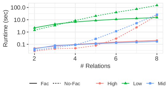
Figure 23. Run time of total count query with (JT)/without message passing (No-JT) in seconds (log scale). High, Mid, and Low are for different fanouts.

D.3.1. Message Passing Costs

We first evaluate the benefits of message passing (but not calibration) in cloud settings. The compiler generates CREATE VIEW statements, so that messages are not materialized. We execute the total count query as a large join-aggregation query (No-JT) or as an upward message passing (JT).

Figure 23 varies the number of relations (x-axis) and fanout (line marker). Message passing reduces the runtimes from exponential to linear due to early marginalization, but incurs a small overhead to perform marginalization when there are few relations. Low fan-out has the largest runtime because we fix the total join size and hence the low fan-out has the largest domain size. Note that the x-axis is also interpretable as the Steiner tree size.

For message passing, we can also interpret number of relations as the Steiner tree size, and the run time grows linearly in the Steiner tree size when the bag size is constant.

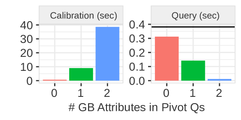
Figure 24. We vary the dimensionality of the calibrated pivot queries $k\in\{0,1,2\}$ and measure calibration runtime and impact on 4-attribute OLAP queries. Horizontal line represents the average runtime with JT.

D.3.2. Cubes in the Cloud

CJTs help developers build data cubes to explicitly trade-off build costs and query performance. To evaluate this, we use the synthetic dataset with $f=10$ (high) fanout and $r=8$ relations, and calibrate all cuboids with $k\in[1,3]$ grouping attributes. For each $k$, we use the cuboids to execute 100 random OLAP queries with 4 grouping attributes.

The results are in Figure 24. Although calibration cost increases exponentially (as expected), message passing is still significantly faster than naive query execution: computing all 2-attribute cuboids (through calibration of all 1 group-by attribute Pivot Qs in $8.8$s) is substantially faster than naively computing a single 0-attribute cuboid ($22.6$s for No-JT in Figure 23). At the same time, increasing the dimensionality of the cuboids ($k$) significantly reduces the query runtimes ($2.71\times$ speedup for $k=1$, and $33.73\times$ speedup for $k=2$) due to the smaller Steiner tree.

The total Redshift table sizes created during calibration is exponential in $k$, and consistent with the analysis in Section D.1. Redshift appears to pad small tables to ${>}6MB$, hence the large sizes (${\sim}4GB$ for $k=2$). Unfortunately. the tables cannot be naively compacted (by unioning into a single table) because their schemas are different. Thus we report the actual Data Size by adding tuple size times cardinality across the tables. The overhead is only $0.17\times$ for $k=0$, $5\times$ for $k=1$ and $127.73\times$ for $k=2$. Given the significant query performance improvement, the space-time trade-off may be worthwhile.

Takeaways. For CJT, the calibration time grows exponentially in the number of group-by attributes, as there are exponential more pivot queries to calibrate, each takes longer time for larger messages. CJT is much more efficient than data cube: CJT can compute all data cuboids up to two group-by attributes in 8.8s, while data cube with naive join takes 22.6s just to compute apex cuboid (Figure 23). The larger number of group-by attributes improves the future OLAP queries performance significantly by reducing Steiner tree size. The reduction of Steiner tree size is especially significant for pivot queries of 2 group-by attributes: given 4 random attributes, there is a high chance ($\sim 90\%$) that two of them are in the same relation so only a scan over absorption is needed.

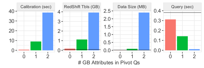
Figure 25. RedShift pads tables to be at least $6MB$, which penalizes many small tables. So we report the total RedShift table size, and actual data size. Horizontal lines represent, from left-to-right: base DB table size, base DB actual data size, and average runtime with JT

The total Redshift table sizes created during calibration is exponential in $k$, and consistent with the analysis in Section D.1. Redshift appears to pad small tables to ${>}6MB$, hence the large sizes (${\sim}4GB$ for $k=2$). Unfortunately. the tables cannot be naively compacted (by unioning into a single table) because their schemas are different. Thus we report the actual Data Size by adding tuple size times cardinality across the tables. The overhead is only $0.17\times$ for $k=0$, $5\times$ for $k=1$ and $127.73\times$ for $k=2$. Given the significant query performance improvement, the space-time trade-off may be worthwhile.

Appendix E TPC-H details

We discussed how we rewrite TPC-H queries into semi-ring SPJA queries.

Query 3. We remove top and order-by. We also remove $L_{O}RDERKEY$ group-by because otherwise the result has too many groups.

SELECT¯SUM(L_EXTENDEDPRICE*(1-L_DISCOUNT))¯AS REVENUE,
O_ORDERDATE, O_SHIPPRIORITY
FROM¯CUSTOMER, ORDERS, LINEITEM
WHERE¯C_MKTSEGMENT¯= ’FURNITURE’ AND
C_CUSTKEY¯= O_CUSTKEY AND L_ORDERKEY¯= O_ORDERKEY AND
O_ORDERDATE¯< ’1995-03-28’ AND L_SHIPDATE¯> ’1995-03-28’
GROUP¯BY¯O_ORDERDATE, O_SHIPPRIORITY;

Query 4. We rewrite the nested query and remove order-by and distinct.

SELECT¯O_ORDERPRIORITY, count(distinct  O_ORDERKEY)
FROM¯LINEITEM, ORDERS
WHERE¯O_ORDERDATE¯>= ’1997-04-01’ AND
¯O_ORDERDATE¯< cast (date ’1997-04-01’ + interval ’3 months’ as date)
AND L_ORDERKEY¯= O_ORDERKEY AND L_COMMITDATE¯< L_RECEIPTDATE
GROUP¯BY¯O_ORDERPRIORITY;

Query 5. For query 5, we break cycle with additional optimization.

SELECT¯N_NATIONKEY,
¯SUM(L_EXTENDEDPRICE*(1-L_DISCOUNT))¯AS REVENUE
FROM¯CUSTOMER, ORDERS, LINEITEM, SUPPLIER, NATION, REGION
WHERE¯C_CUSTKEY¯= O_CUSTKEY AND¯L_ORDERKEY¯= O_ORDERKEY AND
¯L_SUPPKEY¯= S_SUPPKEY AND¯C_NATIONKEY¯= S_NATIONKEY AND
¯S_NATIONKEY¯= N_NATIONKEY AND¯N_REGIONKEY¯= R_REGIONKEY AND
¯R_NAME¯¯= ’MIDDLE EAST’ AND  o_orderdate >= date ’1994-01-01’ AND
o_orderdate < cast (date ’1994-01-01’ + interval ’1 year’ as date)
GROUP¯BY¯N_NATIONKEY;

Break cycle for $Q_{5}$. $Q_{5}$ joins customer and supplier by nation, which makes the join graph cyclic and JT expensive. Luckily, $Q_{5}$ also group-by nation. We discuss the technique to break cycle: rewrite join + group-by as a set of selections.

Consider the cyclic join of R(A,B), S(A,C), T(B,C). If we know that all future queries will group-by attribute A, we can break the cycle through query rewriting. The original join query is:

SELECT A, COUNT(*)
FROM R(A,B), S(A,C), T(B,C)
WHERE R.A = S.A AND R.B = T.B AND S.C = T.C
GROUP BY R.A

The group by query could be considered as a set of smaller queries, each select a value of A in its domain dom(A). Therefore, for each $a\in dom(A)$, we query

SELECT COUNT(*)
FROM R(A,B), S(A,C), T(B,C)
WHERE R.A = S.A AND R.B = T.B AND S.C = T.C AND R.A = a AND S.A = a

The rewritten query has acyclic join graph. This optimization is closely related to conditioning in Probabilistic graphical model [43].

Query 8. We only consider the inner query, as outer query is cheap to compute.

SELECT¯extract(year from o_orderdate) as o_year,
SUM(L_EXTENDEDPRICE * (1-L_DISCOUNT)), N2.N_NATIONKEY
FROM¯PART, SUPPLIER, LINEITEM, ORDERS,
CUSTOMER, NATION N1, NATION N2, REGION
WHERE¯P_PARTKEY¯= L_PARTKEY AND S_SUPPKEY¯= L_SUPPKEY AND
¯¯L_ORDERKEY¯= O_ORDERKEY AND O_CUSTKEY¯= C_CUSTKEY AND
¯¯C_NATIONKEY¯= N1.N_NATIONKEY AND N1.N_REGIONKEY¯= R_REGIONKEY AND
¯¯R_NAME¯¯= ’ASIA’ AND S_NATIONKEY¯= N2.N_NATIONKEY AND
¯¯O_ORDERDATE¯BETWEEN ’1995-01-01’ AND ’1996-12-31’ AND
¯¯P_TYPE¯¯= ’MEDIUM ANODIZED COPPER’
GROUP BY N2.N_NATIONKEY, o_year;

Query 9. We remove the order-by.

SELECT¯N_NAMEAS NATION,
extract(year from o_orderdate) as o_year,
SUM(L_EXTENDEDPRICE*(1-L_DISCOUNT)-PS_SUPPLYCOST*L_QUANTITY)
FROM PART, SUPPLIER, LINEITEM, PARTSUPP, ORDERS, NATION
WHERE S_SUPPKEY¯= L_SUPPKEY AND PS_SUPPKEY¯= L_SUPPKEY
AND PS_PARTKEY¯= L_PARTKEY AND P_PARTKEY¯= L_PARTKEY
AND O_ORDERKEY¯= L_ORDERKEY AND S_NATIONKEY = N_NATIONKEY
AND P_NAME¯LIKE ’%green%’
GROUP BY¯NATION, O_YEAR

Query 10. We remove the limit, order-by and modify the interval to 1 day because otherwise, the result size is too large to return without materialization.

SELECT C_CUSTKEY, C_NAME, SUM(L_EXTENDEDPRICE*(1-L_DISCOUNT))¯AS REVENUE, C_ACCTBAL, N_NAME, C_ADDRESS, C_PHONE, C_COMMENT
FROM CUSTOMER, ORDERS, LINEITEM, NATION
WHERE C_CUSTKEY¯= O_CUSTKEY¯ AND L_ORDERKEY¯= O_ORDERKEY¯¯AND O_ORDERDATE¯>= ’1994-01-01’
AND O_ORDERDATE < cast (date ’1994-01-01’ + interval ’1 days’
as date) AND L_RETURNFLAG = ’R’¯AND C_NATIONKEY¯= N_NATIONKEY
GROUP BY C_CUSTKEY, C_NAME, C_ACCTBAL,
C_PHONE, N_NAME, C_ADDRESS, C_COMMENT

References

- [1] Looker. https://www.looker.com/.
- [2] Corporación favorita grocery sales forecasting. https://www.kaggle.com/c/favorita-grocery-sales-forecasting, 10 2017.
- [3] Modin: Scale your pandas workflows by changing one line of code. https://github.com/modin-project/modin, 2018.
- [4] C. R. Aberger, A. Lamb, S. Tu, A. Nötzli, K. Olukotun, and C. Ré. Emptyheaded: A relational engine for graph processing. ACM Transactions on Database Systems (TODS), 42(4):1–44, 2017.
- [5] M. Abo Khamis, H. Q. Ngo, and A. Rudra. Faq: questions asked frequently. In Proceedings of the 35th ACM SIGMOD-SIGACT-SIGAI Symposium on Principles of Database Systems, pages 13–28, 2016.
- [6] M. Abo Khamis, H. Q. Ngo, and D. Suciu. Computing join queries with functional dependencies. In Proceedings of the 35th ACM SIGMOD-SIGACT-SIGAI Symposium on Principles of Database Systems, pages 327–342, 2016.
- [7] M. Abourezq and A. Idrissi. Database-as-a-service for big data: An overview. International Journal of Advanced Computer Science and Applications, 7(1), 2016.
- [8] M. Ahmad, M. A. Qadir, A. Rahman, R. Zagrouba, F. Alhaidari, T. Ali, and F. Zahid. Enhanced query processing over semantic cache for cloud based relational databases. Journal of Ambient Intelligence and Humanized Computing, pages 1–19, 2020.
- [9] M.-C. Albutiu, A. Kemper, and T. Neumann. Massively parallel sort-merge joins in main memory multi-core database systems. arXiv preprint arXiv:1207.0145, 2012.
- [10] Z. Asgharzadeh Talebi, R. Chirkova, and Y. Fathi. Exact and inexact methods for solving the problem of view selection for aggregate queries. International Journal of Business Intelligence and Data Mining, 4(3-4):391–415, 2009.
- [11] A. Atserias, M. Grohe, and D. Marx. Size bounds and query plans for relational joins. In 2008 49th Annual IEEE Symposium on Foundations of Computer Science, pages 739–748. IEEE, 2008.
- [12] O. Bashaw. Drive revenue by using sigma with salesforce. https://www.sigmacomputing.com/blog/drive-revenue-by-using-sigma-with-salesforce, 2022.
- [13] T. Braun and R. Möller. Lifted junction tree algorithm. In Joint German/Austrian Conference on Artificial Intelligence (Künstliche Intelligenz), pages 30–42. Springer, 2016.
- [14] S. Chaudhuri, R. Krishnamurthy, S. Potamianos, and K. Shim. Optimizing queries with materialized views. In Proceedings of the Eleventh International Conference on Data Engineering, pages 190–200. IEEE, 1995.
- [15] N. Chepurko, R. Marcus, E. Zgraggen, R. C. Fernandez, T. Kraska, and D. Karger. Arda: automatic relational data augmentation for machine learning. arXiv preprint arXiv:2003.09758, 2020.
- [16] D. Conaty, D. D. Mauá, and C. P. De Campos. Approximation complexity of maximum a posteriori inference in sum-product networks. arXiv preprint arXiv:1703.06045, 2017.
- [17] G. Cormode. Sketch techniques for approximate query processing. Foundations and Trends in Databases. NOW publishers, page 15, 2011.
- [18] F. G. Cozman et al. Generalizing variable elimination in bayesian networks. In Workshop on probabilistic reasoning in artificial intelligence, pages 27–32. Citeseer, 2000.
- [19] R. Curtin, B. Moseley, H. Ngo, X. Nguyen, D. Olteanu, and M. Schleich. Rk-means: Fast clustering for relational data. In International Conference on Artificial Intelligence and Statistics, pages 2742–2752. PMLR, 2020.
- [20] F. Dehne, T. Eavis, S. Hambrusch, and A. Rau-Chaplin. Parallelizing the data cube. Distributed and Parallel Databases, 11(2):181–201, 2002.
- [21] J. Deng, N. Ding, Y. Jia, A. Frome, K. Murphy, S. Bengio, Y. Li, H. Neven, and H. Adam. Large-scale object classification using label relation graphs. In European conference on computer vision, pages 48–64. Springer, 2014.
- [22] D. Donjerkovic and R. Ramakrishnan. Probabilistic optimization of top n queries. Technical report, University of Wisconsin-Madison Department of Computer Sciences, 1999.
- [23] P. Eichmann, E. Zgraggen, C. Binnig, and T. Kraska. Idebench: A benchmark for interactive data exploration. In Proceedings of the 2020 ACM SIGMOD International Conference on Management of Data, pages 1555–1569, 2020.
- [24] R. C. Fernandez, Z. Abedjan, F. Koko, G. Yuan, S. Madden, and M. Stonebraker. Aurum: A data discovery system. In 2018 IEEE 34th International Conference on Data Engineering (ICDE), pages 1001–1012. IEEE, 2018.
- [25] R. C. Fernandez, P. Subramaniam, and M. J. Franklin. Data market platforms: Trading data assets to solve data problems. arXiv preprint arXiv:2002.01047, 2020.
- [26] A. Ferrari and M. Russo. Introducing Microsoft Power BI. Microsoft Press, 2016.
- [27] W. Fischl, G. Gottlob, and R. Pichler. General and fractional hypertree decompositions: Hard and easy cases. In Proceedings of the 37th ACM SIGMOD-SIGACT-SIGAI Symposium on Principles of Database Systems, pages 17–32, 2018.
- [28] J. Gale, M. Seiden, G. Atwood, J. Frantz, R. Woollen, and Ç. Demiralp. Sigma worksheet: Interactive construction of olap queries. arXiv preprint arXiv:2012.00697, 2020.
- [29] J. Gray, S. Chaudhuri, A. Bosworth, A. Layman, D. Reichart, M. Venkatrao, F. Pellow, and H. Pirahesh. Data cube: A relational aggregation operator generalizing group-by, cross-tab, and sub-totals. Data mining and knowledge discovery, 1(1):29–53, 1997.
- [30] T. J. Green, G. Karvounarakis, and V. Tannen. Provenance semirings. In Proceedings of the twenty-sixth ACM SIGMOD-SIGACT-SIGART symposium on Principles of database systems, pages 31–40, 2007.
- [31] J. Gryz. Query folding with inclusion dependencies. In Proceedings 14th International Conference on Data Engineering, pages 126–133. IEEE, 1998.
- [32] S. Guo, W. Sun, and M. A. Weiss. On satisfiability, equivalence, and implication problems involving conjunctive queries in database systems. IEEE Transactions on Knowledge and Data Engineering, 8(4):604–616, 1996.
- [33] A. Gupta, V. Harinarayan, and D. Quass. Aggregate-query processing in data warehousing environments. 1995.
- [34] A. Gupta, I. S. Mumick, and K. A. Ross. Adapting materialized views after redefinitions. In Proceedings of the 1995 ACM SIGMOD international conference on Management of data, pages 211–222, 1995.
- [35] J. Han, N. Stefanovic, and K. Koperski. Selective materialization: An efficient method for spatial data cube construction. In Pacific-Asia conference on knowledge discovery and data mining, pages 144–158. Springer, 1998.
- [36] M. Hong, M. Riedewald, C. Koch, J. Gehrke, and A. Demers. Rule-based multi-query optimization. In Proceedings of the 12th International Conference on Extending Database Technology: Advances in Database Technology, pages 120–131, 2009.
- [37] M. Idris, M. Ugarte, and S. Vansummeren. The dynamic yannakakis algorithm: Compact and efficient query processing under updates. In Proceedings of the 2017 ACM International Conference on Management of Data, pages 1259–1274, 2017.
- [38] M. Joglekar, R. Puttagunta, and C. Ré. Aggregations over generalized hypertree decompositions. arXiv preprint arXiv:1508.07532, 2015.
- [39] M. R. Joglekar, R. Puttagunta, and C. Ré. Ajar: Aggregations and joins over annotated relations. In Proceedings of the 35th ACM SIGMOD-SIGACT-SIGAI Symposium on Principles of Database Systems, pages 91–106, 2016.
- [40] H. F. Kaiser and K. Dickman. Sample and population score matrices and sample correlation matrices from an arbitrary population correlation matrix. Psychometrika, 27(2):179–182, 1962.
- [41] M. A. Khamis, R. R. Curtin, B. Moseley, H. Q. Ngo, X. Nguyen, D. Olteanu, and M. Schleich. Functional aggregate queries with additive inequalities. ACM Transactions on Database Systems (TODS), 45(4):1–41, 2020.
- [42] M. A. Khamis, H. Q. Ngo, X. Nguyen, D. Olteanu, and M. Schleich. Ac/dc: In-database learning thunderstruck. In Proceedings of the Second Workshop on Data Management for End-To-End Machine Learning, pages 1–10, 2018.
- [43] D. Koller and N. Friedman. Probabilistic graphical models: principles and techniques. MIT press, 2009.
- [44] N. Kotsis and D. R. McGregor. Elimination of redundant views in multidimensional aggregates. In International Conference on Data Warehousing and Knowledge Discovery, pages 146–161. Springer, 2000.
- [45] S. L. Lauritzen and N. A. Sheehan. Graphical models for genetic analyses. Statistical Science, pages 489–514, 2003.
- [46] V. Leis, B. Radke, A. Gubichev, A. Mirchev, P. Boncz, A. Kemper, and T. Neumann. Query optimization through the looking glass, and what we found running the join order benchmark. The VLDB Journal, 27(5):643–668, 2018.
- [47] J. Li, Z. A. Talebi, R. Chirkova, and Y. Fathi. A formal model for the problem of view selection for aggregate queries. In East European Conference on Advances in Databases and Information Systems, pages 125–138. Springer, 2005.
- [48] L. Lins, J. T. Klosowski, and C. Scheidegger. Nanocubes for real-time exploration of spatiotemporal datasets. IEEE Transactions on Visualization and Computer Graphics, 19(12):2456–2465, 2013.
- [49] Z. Liu and J. Heer. The effects of interactive latency on exploratory visual analysis. IEEE transactions on visualization and computer graphics, 20(12):2122–2131, 2014.
- [50] Z. Liu, B. Jiang, and J. Heer. immens: Real-time visual querying of big data. In Computer Graphics Forum, volume 32, pages 421–430. Wiley Online Library, 2013.
- [51] D. Moritz, B. Howe, and J. Heer. Falcon: Balancing interactive latency and resolution sensitivity for scalable linked visualizations. In Proceedings of the 2019 CHI Conference on Human Factors in Computing Systems, pages 1–11, 2019.
- [52] E. G. Morton-Owens and K. L. Hanson. Trends at a glance: A management dashboard of library statistics. Information Technology and Libraries, 31(3):36–51, 2012.
- [53] T. Neumann and B. Radke. Adaptive optimization of very large join queries. In Proceedings of the 2018 International Conference on Management of Data, pages 677–692, 2018.
- [54] H. Q. Ngo, E. Porat, C. Ré, and A. Rudra. Worst-case optimal join algorithms. Journal of the ACM (JACM), 65(3):1–40, 2018.
- [55] M. Nikolic and D. Olteanu. Incremental view maintenance with triple lock factorization benefits. In Proceedings of the 2018 International Conference on Management of Data, pages 365–380, 2018.
- [56] B. of Transportation Statisticsw. Bureau of transportation statistics. http://www.transtats.bts.gov, 2017.
- [57] D. Olteanu and J. Závodnỳ. Size bounds for factorised representations of query results. ACM Transactions on Database Systems (TODS), 40(1):1–44, 2015.
- [58] C. A. Pahins, S. A. Stephens, C. Scheidegger, and J. L. Comba. Hashedcubes: Simple, low memory, real-time visual exploration of big data. IEEE transactions on visualization and computer graphics, 23(1):671–680, 2016.
- [59] T. pandas development team. pandas-dev/pandas: Pandas, Feb. 2020.
- [60] J. Pearl. Reverend Bayes on inference engines: A distributed hierarchical approach. Cognitive Systems Laboratory, School of Engineering and Applied Science …, 1982.
- [61] A. L. Pineda and V. Gopalakrishnan. Novel application of junction trees to the interpretation of epigenetic differences among lung cancer subtypes. AMIA Summits on Translational Science Proceedings, 2015:31, 2015.
- [62] M. Raasveldt and H. Mühleisen. Duckdb: an embeddable analytical database. In Proceedings of the 2019 International Conference on Management of Data, pages 1981–1984, 2019.
- [63] J. C. Ramirez, G. Munoz, and L. Gutierrez. Fault diagnosis in an industrial process using bayesian networks: Application of the junction tree algorithm. In 2009 Electronics, Robotics and Automotive Mechanics Conference (CERMA), pages 301–306. IEEE, 2009.
- [64] Q. Ren, M. H. Dunham, and V. Kumar. Semantic caching and query processing. IEEE transactions on knowledge and data engineering, 15(1):192–210, 2003.
- [65] I. Robinson, J. Webber, and E. Eifrem. Graph databases: new opportunities for connected data. " O’Reilly Media, Inc.", 2015.
- [66] P. Roy, S. Seshadri, S. Sudarshan, and S. Bhobe. Efficient and extensible algorithms for multi query optimization. In Proceedings of the 2000 ACM SIGMOD international conference on Management of data, pages 249–260, 2000.
- [67] M. Schleich. Structure-aware machine learning over multi-relational databases. In Proceedings of the 2021 International Conference on Management of Data, pages 6–7, 2021.
- [68] M. Schleich, D. Olteanu, M. Abo Khamis, H. Q. Ngo, and X. Nguyen. A layered aggregate engine for analytics workloads. In Proceedings of the 2019 International Conference on Management of Data, pages 1642–1659, 2019.
- [69] M. Schleich, D. Olteanu, and R. Ciucanu. Learning linear regression models over factorized joins. In Proceedings of the 2016 International Conference on Management of Data, pages 3–18, 2016.
- [70] P. G. Selinger, M. M. Astrahan, D. D. Chamberlin, R. A. Lorie, and T. G. Price. Access path selection in a relational database management system. In Proceedings of the 1979 ACM SIGMOD international conference on Management of data, pages 23–34, 1979.
- [71] G. R. Shafer and P. P. Shenoy. Probability propagation. Annals of mathematics and Artificial Intelligence, 2(1):327–351, 1990.
- [72] M. Steinbrunn, G. Moerkotte, and A. Kemper. Heuristic and randomized optimization for the join ordering problem. The VLDB Journal, 6:191–208, 1997.
- [73] D. Taniar and R. B.-N. Tan. Parallel processing of multi-join expansion-aggregate data cube query in high performance database systems. In Proceedings International Symposium on Parallel Architectures, Algorithms and Networks. I-SPAN’02, pages 51–56. IEEE, 2002.
- [74] D. Theodoratos and W. Xu. Constructing search spaces for materialized view selection. In Proceedings of the 7th ACM international workshop on Data warehousing and OLAP, pages 112–121, 2004.
- [75] T. L. Veldhuizen. Leapfrog triejoin: A simple, worst-case optimal join algorithm. arXiv preprint arXiv:1210.0481, 2012.
- [76] J. S. Vitter, M. Wang, and B. Iyer. Data cube approximation and histograms via wavelets. In Proceedings of the seventh international conference on Information and knowledge management, pages 96–104, 1998.
- [77] M. J. Wainwright, T. S. Jaakkola, and A. S. Willsky. Map estimation via agreement on trees: message-passing and linear programming. IEEE transactions on information theory, 51(11):3697–3717, 2005.
- [78] W. Wang, J. Feng, H. Lu, and J. X. Yu. Condensed cube: An effective approach to reducing data cube size. In Proceedings 18th International Conference on Data Engineering, pages 155–165. IEEE, 2002.
- [79] Z. Wang, Y. Chu, K.-L. Tan, D. Agrawal, A. E. Abbadi, and X. Xu. Scalable data cube analysis over big data. arXiv preprint arXiv:1311.5663, 2013.
- [80] D. Wu and L. Wu. Hierarchical junction trees as the secondary structure for inference in bayesian networks. In Eighth ACIS International Conference on Software Engineering, Artificial Intelligence, Networking, and Parallel/Distributed Computing (SNPD 2007), volume 3, pages 706–712. IEEE, 2007.
- [81] K. Xirogiannopoulos and A. Deshpande. Memory-efficient group-by aggregates over multi-way joins. arXiv preprint arXiv:1906.05745, 2019.
- [82] M. Yannakakis. Algorithms for acyclic database schemes. In VLDB, volume 81, pages 82–94, 1981.
- [83] C. T. Yu and M. Z. Ozsoyoglu. An algorithm for tree-query membership of a distributed query. In COMPSAC 79. Proceedings. Computer Software and The IEEE Computer Society’s Third International Applications Conference, 1979., pages 306–312. IEEE, 1979.
- [84] Q. Zhou, J. Arulraj, S. Navathe, W. Harris, and D. Xu. Automated verification of query equivalence using satisfiability modulo theories. Proceedings of the VLDB Endowment, 12(11):1276–1288, 2019.
- [85] F. Zhu, H. A. Aziz, X. Qian, and S. V. Ukkusuri. A junction-tree based learning algorithm to optimize network wide traffic control: A coordinated multi-agent framework. Transportation Research Part C: Emerging Technologies, 58:487–501, 2015.